VARIABLE RESOLUTION METHODS IN FV3

Lucas Harris

and the GFDL FV3 Team

FV3 Workshop in Taiwan

4 December 2017

HIGH RESOLUTION MODELING:LIMITED AREA VS. GLOBAL MODELS

• Stand-alone regional models are commonly used for mesoscale simulation and regional climate modeling. But boundary errors creep in after a few days.

• Require potentially inconsistent BCs from a global model.

• No feedback onto large-scale

• Global models have no boundaries and are globally consistent, but global high resolution can be impractical

• Solution: grid refinement of a global model!

GRID REFINEMENT

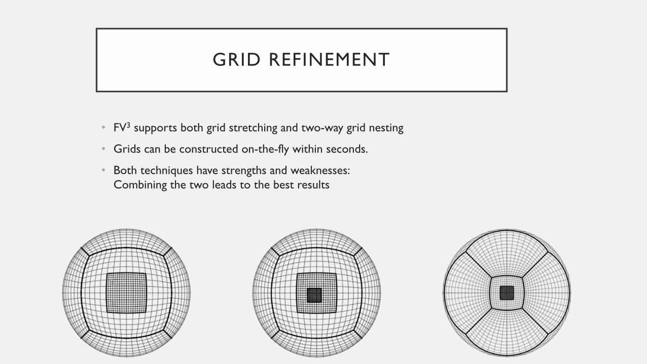
• FV3 supports both grid stretching and two-way grid nesting

• Grids can be constructed on-the-fly within seconds.

• Both techniques have strengths and weaknesses:Combining the two leads to the best results

• The simple, easy way to achieve grid refinement

• Smooth deformation! Requires no changes to the solver

• No abrupt discontinuity.

• Capable of extreme refinement (80x!!) for easy storm-scale simulations on a full-size earth

• Requires a “compromise” tuning between coarse and fine regions. (A good scale-aware scheme can help here.)

STRETCHED GRID

SCHMIDT TRANSFORMATION

• Smoothly deforms the cubed sphere into a “truncated pyramid”, with the high-resolution face at the top of the “pyramid”

• Transformation is analytic. Easily implemented and quickly executed

• The resulting pyramid can then be rotated to an arbitrary target point

• Transformation does coarsen the opposing side of the sphere

• Size of high-resolution region decreaseswith increasing stretching ratio

of Lin et al. (1983). The surface flux, boundary layer, orographic gravity wave drag, and108

radiative transfer parameterizations are the same as in GFDL AM2.1 (GFDL Global At-109

mosphere Model Development Team, 2004), although the timestep at which the radiative110

tendencies are computed has been decreased from three hours to one hour, and there is no111

convective gravity wave drag parameterization. Aerosols, ozone, and well-mixed greenhouse112

gases are prescribed; there are no interactive aerosols or aerosol indirect e↵ect.113

a. The Schmidt Transformation114

The transformation of Schmidt (1977) provides a smooth, analytic means of deforming115

any spherical grid by “attracting” grid points to a specified central location, which can then116

be rotated to any other point on the sphere using a solid-body rotation. In this method,117

grid points of the original cubed sphere are attracted to the south pole, so that we need118

only do the stretching along meridians, leaving longitudes unchanged; the south pole is then119

moved to the target latitude and longitude by a solid-body rotation. The transformation of120

the latitude ✓ to # by stretching is given by121

sin # =D + sin ✓

1 + D sin ✓D =

1� c2

1 + c2, (1)

where c is the stretching factor, which can be any positive real number. The stretching is122

smooth, so that the grid-cell-width varies smoothly outward from the refined region, unlike123

the abrupt refinement resulting from grid nesting. However, the Schmidt transformation also124

leaves a lower-resolution region on the opposite side of the sphere, which covers more than125

half of the earth’s area. (We will find that this degraded-resolution area does not adversely126

a↵ect the quality of HiRAM’s global climate.) The outline of the resulting stretched grid127

resembles a “flower” with four petals, the center of which is the highest-resolution area.128

The di↵erence between stretched and (quasi-)uniform resolution can be seen in Figure 1,129

in which an undeformed c384 (25 km) grid (Figure 1a) is deformed by a factor of 2.5 and130

rotated to two di↵erent locations, Oklahoma City (henceforth “OKC”, 35.4 N, 97.6 W;131

5

of Lin et al. (1983). The surface flux, boundary layer, orographic gravity wave drag, and108

radiative transfer parameterizations are the same as in GFDL AM2.1 (GFDL Global At-109

mosphere Model Development Team, 2004), although the timestep at which the radiative110

tendencies are computed has been decreased from three hours to one hour, and there is no111

convective gravity wave drag parameterization. Aerosols, ozone, and well-mixed greenhouse112

gases are prescribed; there are no interactive aerosols or aerosol indirect e↵ect.113

a. The Schmidt Transformation114

The transformation of Schmidt (1977) provides a smooth, analytic means of deforming115

any spherical grid by “attracting” grid points to a specified central location, which can then116

be rotated to any other point on the sphere using a solid-body rotation. In this method,117

grid points of the original cubed sphere are attracted to the south pole, so that we need118

only do the stretching along meridians, leaving longitudes unchanged; the south pole is then119

moved to the target latitude and longitude by a solid-body rotation. The transformation of120

the latitude ✓ to # by stretching is given by121

sin # =D + sin ✓

1 + D sin ✓D =

1� c2

1 + c2, (1)

where c is the stretching factor, which can be any positive real number. The stretching is122

smooth, so that the grid-cell-width varies smoothly outward from the refined region, unlike123

the abrupt refinement resulting from grid nesting. However, the Schmidt transformation also124

leaves a lower-resolution region on the opposite side of the sphere, which covers more than125

half of the earth’s area. (We will find that this degraded-resolution area does not adversely126

a↵ect the quality of HiRAM’s global climate.) The outline of the resulting stretched grid127

resembles a “flower” with four petals, the center of which is the highest-resolution area.128

The di↵erence between stretched and (quasi-)uniform resolution can be seen in Figure 1,129

in which an undeformed c384 (25 km) grid (Figure 1a) is deformed by a factor of 2.5 and130

rotated to two di↵erent locations, Oklahoma City (henceforth “OKC”, 35.4 N, 97.6 W;131

5

TWO-WAY GRID NESTING

• Simultaneous coupled, consistent global and regional solution. No waiting for a regional prediction!

• Different grids permit different parameterizations and timesteps; doesn’t need a “compromise” for high-resolution region

• Flexible! Great possibilities for combining nesting and stretching.

GRID NESTING: BOUNDARY CONDITIONS

• Strategy: fill halo (ghost) cells with boundary conditionsInterior of solver needs no changes

• All variables linearly interpolated in space into nested grid halo. Correct upwind BCs “baked in” by FV’s upstream-biased fluxes

• BCs for all solution variables, as well as C-grid winds, and divergence

• Nonhydrostatic solver requires nonhydrostatic pressure, computed using the semi-implicit solver—consistent with interior algorithm

GRID NESTING: BOUNDARY CONDITIONS

• Concurrent nesting: BCs extrapolated in time so nest and coarse grids can run simultaneously.

• BCs stepped forward every acoustic timestep

• New BC data updated at the nest interaction frequency,usually vertical remap frequency

• Extrapolation is formally unstable but is not a problem in practice

• Option to limit extrapolation to ensure positivity for scalars

• Two-time level extrapolation requires saving BCs across restarts to ensure run-to-run reproducibility

GRID NESTINGTOPOGRAPHY AND SMOOTHING

• FV3 applies no additional diffusion or relaxation at the boundaries

• Linear interpolation introduces some smoothing without creating new extrema

• For consistency, halo topography is linearly interpolated from the coarse grid, the same way as the solution variables

• Topography near the boundary is blended with the interpolated coarse-grid topography

TWO-WAY INTERACTION

• Two-way nesting: coarse grid solution periodically replaced (“updated”) by nested-grid solution where the grids coincide

• Essential for small-to-large-scale interaction (e.g. hurricanes, gravity-wave drag, small-scale orographic/coastal processes)

• Theory suggests two-way nesting yields a better nested-grid solution: Harris and Durran (2010), T.T. Warner et al (1997)

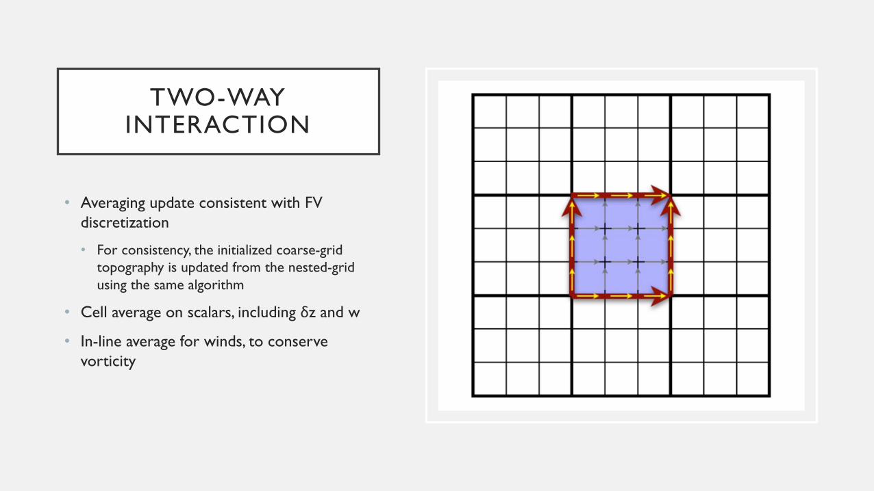
TWO-WAYINTERACTION

• Averaging update consistent with FV discretization

• For consistency, the initialized coarse-grid topography is updated from the nested-grid using the same algorithm

• Cell average on scalars, including δz and w

• In-line average for winds, to conserve vorticity

MASS CONSERVATION AND TWO-WAY NESTING

• Conservation usually requires flux BCs at the nested-grid boundaryThese are difficult to implement with the time-extrapolation BC

• Our approach: Update everything except mass (δp) and tracers

• Very simple!Works regardless of BC and grid alignment

• Two-way nesting over-specifies coarse-grid solution Less updating, less over-specification

MASS CONSERVATION AND TWO-WAY NESTING

• Our approach: Update everything except mass (δp) and tracers

• Because δp is the vertical coordinate, we then need to remap the nested-grid data to the coarse grid’s vertical coordinate

• Under development: “Renormalization-update” for tracers uses a layer-by-layer fixer to ensure tracer mass conservation

TWO-WAY VS . ONE-WAY GRID

NESTING

• GFDL HiRAM climate model

c90 (1°) and c90n3 (1° and 1/3°)

CMAP DJF Observations

1° uniform AMIP

One-way 1/3° climo SST

Two-way 1/3° AMIP

mm/d

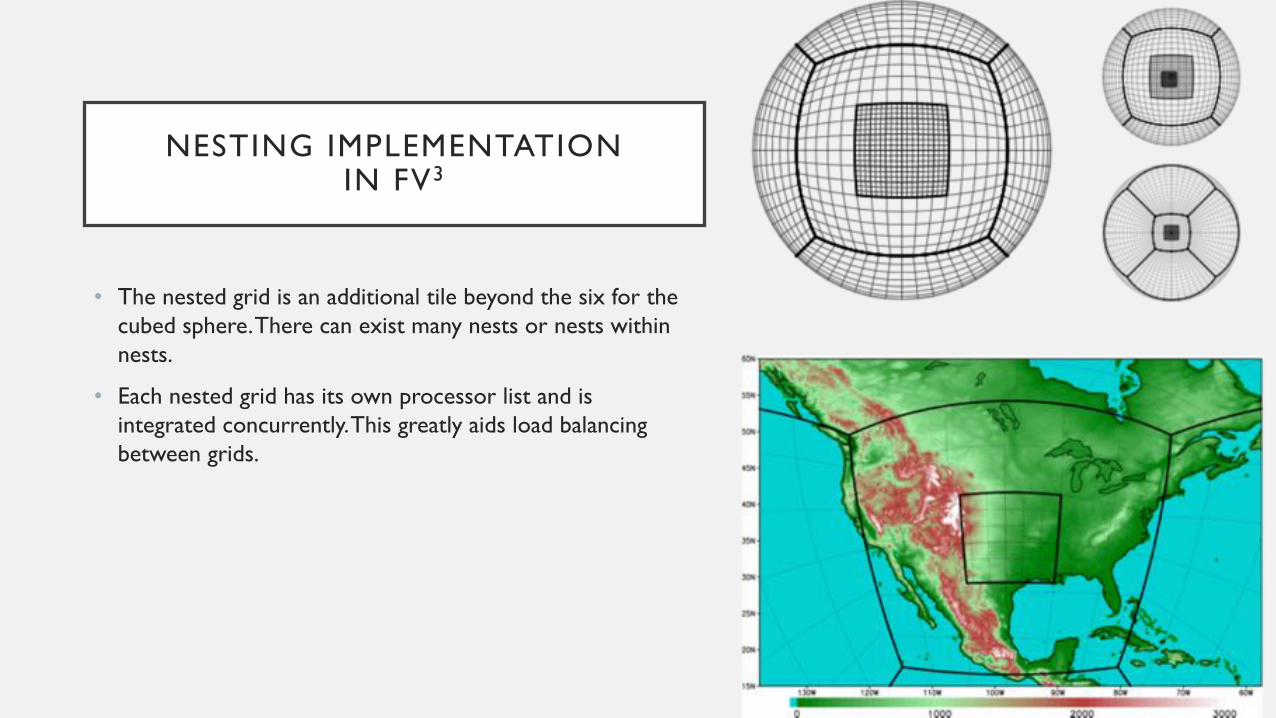
NESTING IMPLEMENTATIONIN FV3

• The nested grid is an additional tile beyond the six for the cubed sphere. There can exist many nests or nests within nests.

• Each nested grid has its own processor list and is integrated concurrently. This greatly aids load balancing between grids.

fv_dynamics()FV3 solver

dyn_core()Lagrangian dynamics

fv_tracer2d()Sub-cycled tracer transport

OpenMP on k

Lagrangian_to_Eulerian()Vertical Remapping(i,k) OpenMP on j

c_sw(), etc.C-grid solver

d_sw()Forward Lagrangian dyn.

OpenMP on k

update_dz_d()Forward δz evaluation

OpenMP on k

one_grad_p()/nh_p_grad()Backwards horizontal PGF

OpenMP on k

riem_solver()Backwards vertical PGF, sound wave processes

(i,k) OpenMP on j

[physics]

fv_update_phys()Consistent field update

dt_atmosk_split

“remapping” loopn_split

“acoustic” loop

Twoway_update()OpenMP on k

fv_dynamics()FV3 solver

dyn_core()Lagrangian dynamics

fv_tracer2d()Sub-cycled tracer transport

OpenMP on k

Lagrangian_to_Eulerian()Vertical Remapping(i,k) OpenMP on j

c_sw(), etc.C-grid solver

d_sw()Forward Lagrangian dyn.

OpenMP on k

update_dz_d()Forward δz evaluation

OpenMP on k

one_grad_p()/nh_p_grad()Backwards horizontal PGF

OpenMP on k

riem_solver()Backwards vertical PGF, sound wave processes

(i,k) OpenMP on j

[physics]

fv_update_phys()Consistent field update

dt_atmosk_split

“remapping” loopn_split

“acoustic” loopsetup_nested_grid_BCs()or setup_regional_BCs()

OpenMP on k

NESTED-GRID WORKFLOW

• Nested grids can be generated online, although orography, land-surface information, and initial conditions have to be generated.

• Modifications of standard NCEP tools allow offline generation of grid information and ICs

• Each grid gets its own namelistAny runtime parameter can be customized for the individual grids

• GFDL fregrid can perform conservative remapping of nested-grid output onto a regional regular latitude-longitude grid. It is also possible to use common software (Python, NCL, IDL, GrADS (?), etc) to plot the native nested grid.