variable resolution spatial interpolation using the simple recursive point voronoi diagram ·...

Variable Resolution Spatial Interpolation

Using the Simple Recursive Point Voronoi

Diagram

Robert Feick,1 Barry Boots2

1Department of Geography, School of Planning, University of Waterloo, Waterloo, ON, Canada,2Department of Geography and Environmental Studies, Wilfrid Laurier University, Waterloo, ON, Canada

This article introduces a procedure for progressively increasing the density of an initial

point set that can be used as a basis for interpolating surfaces of variable resolution

from sparse samples of data sites. The procedure uses the Simple Recursive Point

Voronoi Diagram in which Voronoi concepts are used to tessellate space with respect

to a given set of generator points. The construction is repeated every time with a new

generator set, which comprises members selected from the previous generator set plus

features of the current tessellation. We show how this procedure can be implemented

in Arc/Info and present an illustration of its application using three known surfaces and

alternative generator point configurations. Initial results suggest that the procedure has

considerable potential and we discuss further methods for evaluating and extending it.

Introduction

Spatial data consist of measurements (data values) of an attribute taken at specific

locations (data sites) in a geographic space (study region). In much of the data col-

lected in the environmental sciences, the attribute is assumed to be spatially con-

tinuous (possibly piecewise) so that the data values can be considered as a sampling

of the attribute at the data sites. Suppose that our primary aim is to use the data to

interpolate the values of the attribute at locations other than the data sites, thus

enabling us to create a visual representation of the underlying surface (Watson

1992). This task can be considered as a specific instance of the more general prob-

lem of approximating surfaces that arises in a variety of applications in computer-

aided design, computer graphics, computer vision, and finite element methods. In

some applications, where the number of data sites is very large, it may not be

necessary to use all the data sites in order to capture the fundamental features of the

Correspondence: Robert Feick, Department of Geography, University of Waterloo,Waterloo, Canada ON N2L 3G1e-mail: [email protected]

Submitted: November 11, 2003. Revised version accepted: June 6, 2004.

Geographical Analysis 37 (2005) 225–243 r 2005 The Ohio State University 225

Geographical Analysis ISSN 0016-7363

surface. Instead, a representative subset of data sites, which enables the surface to

be represented with a prespecified level of accuracy, can be selected. This can be

achieved either by a process of simplification (also referred to as decimation or

coarsening) in which we start with the complete set of data sites and remove some

of them or by a process of refinement when we start with an insufficient subset of

data sites and add additional ones (see Garland [1999] and De Floriani and Magillo

[2002] for reviews). However, there are also situations where the data sites are

sparse and there is no possibility of supplementing their number by increasing the

size of the sample. Typically, this applies to most historical data. Further, notwith-

standing advances in remote sensing and global positioning system data collection

methods, in some instances it can still be impractical or too costly to collect ap-

propriately detailed data. In addition, with historical data, we may also lack knowl-

edge of the sampling design, although some characteristics may be inferred from

the spatial distribution of data sites. Much less attention has been applied to this

situation, which is the focus of this article.

We propose a procedure for progressively increasing the density of an initial

point set that provides a basis for interpolating surfaces of variable resolution from

sparse samples of data sites. The procedure makes use of the simple recursive point

Voronoi diagram (SRPVD).

Our proposal is motivated by both practical and conceptual considerations.

Practically, the procedure can be fully automated and implemented within existing

commercial off-the-shelf (COTS) software. Conceptually, it is supported by recog-

nition of the dual relationships between Voronoi and Delaunay constructions. The

latter have a long history of use in terrain modeling and visualization, with the

Delaunay triangulation being the most popular method of constructing a triangu-

lated irregular network (TIN; Hutchinson and Gallant 1999). In part, this is because

it is the only triangulation that satisfies both local and global max–min angle criteria

(Sibson 1978; Okabe et al. 2000, p. 93). Wang et al. (2001) also demonstrate that

the basic Delaunay triangulation even outperforms data-dependent triangulations

in modeling terrain surfaces. Further, several recursive forms of Delaunay triangu-

lations have already been used as top-down, multiresolution TIN models in the

refinement process described above (see De Floriani, Marzano, and Puppo 1996;

De Floriani et al. 2000 for reviews). These include strictly hierarchical TINs

(HTINs), which involve the recursive subdivision of the initial triangle(s) into a

set of nested triangles (De Floriani and Puppo 1992, 1995), and nonnested, py-

ramidal TINs (PTINs) in which a new structure is computed every time new points

are inserted (De Floriani, Falcidieno, and Pienovi 1985; De Floriani 1989; Voight-

mann, Becker, and Hinrichs 1994). It will become apparent below that, in essence,

the SRPVD is a dual form of PTIN.

We begin our presentation by describing recursive Voronoi diagrams in general

terms and providing a specific definition of the SRPVD. We then show how these

constructions can be used to create surfaces of varying spatial resolution. In the

third main section we describe how these procedures can be implemented in Arc/

Geographical Analysis

226

Info. This is followed in the fourth section by an application of the procedure to

point samples drawn from three known topographic surfaces using three different

sampling designs. We conclude by discussing outstanding issues and directions for

future work.

Recursive Voronoi diagrams

The basic Voronoi concept involves tessellating an m-dimensional space with re-

spect to a finite set of objects by assigning all locations in the space to the closest

member of the object set. This concept can also be applied recursively by tessel-

lating the space with respect to a given set of generators and then repeating the

construction every time with a new generator set consisting of objects selected from

the previous generator set plus features of the current tessellation. More formally,

consider a finite set of n distinct generators, G. First, construct the Voronoi diagram

V(G) of G. Next, extract a set of features Q from V(G) and create a new set of gen-

erators G0 that comprises Q plus selected members of G. Then construct the Vor-

onoi diagram V(G0) ofG0. This step is then repeated a number of times. At each step,

the number of generators that are retained may range from none to all. Boots and

Shiode (2003) show that such recursive constructions provide an integrative con-

ceptual framework for a number of disparate procedures in spatial analysis and

modeling.

Simple recursive point Voronoi diagram

In this article, we consider a specific form of recursive Voronoi diagram, the

SRPVD, in which the initial set of generators consists of n distinct points

G(0)5 {g(0)1, g(0)2, . . ., g(0)n}. The construction of this diagram involves the follow-

ing steps:

0. define the initial set of generators G(0);

1. generate the ordinary Voronoi diagram V(G(0)) of G(0);

2. extract all m(0) Voronoi vertices Q(0)5 {q(0)1, q(0)2, . . ., q(0)m(0)} of V(G(0));

3. create a new set of generator points G(1)5G(0)1Q(0); and

4. repeat steps 1 through 3.

We call the result of the kth construction, V(G(k)), the kth generation of the

SRPVD. Similarly, we call its generator set G(k) and its vertices Q(k) the kth gener-

ation of the point set and the kth generation of the vertices, respectively. The

results of applying these steps for five recursions to an initial generator set

consisting of five points are shown in Fig. 1. Note that the Voronoi polygons

at generation k are either entirely contained within a Voronoi polygon at gene-

ration (k� 1), that is, V(G(k)i) � V(G(k� 1)i), or are composed of pieces of three pol-

ygons from generation (k� 1), that is, V(G(k)i)5 (V(G(k)i) \ V(G(k�1)l)) [ (V(G(k)i) \V(G(k� 1)m)) [ (V(G(k)i) \ V(G(k� 1)n)) (see Fig. 2). As noted above, a recursive

Variable Resolution Spatial InterpolationRobert Feick and Barry Boots

227

Voronoi structure will have a dual recursive Delaunay structure. The recursive

Delaunay construction that is equivalent to the SRPVD is defined as follows:

0. define the initial set of generators G(0);

1. generate the Delaunay triangulation D(0) of G(0);

2. identify the circumcenters C(0)5 {c(0)1, . . ., c(0)m} of all the triangles of D(0);

3. create a new set of generator points G(1)5G(0)1C(0); and

4. repeat steps 1 and 3.

Figure 1. The first five recursions of a simple recursive point Voronoi diagram.

Figure 2. Simple recursive point Voronoi diagram generations 1–3.


228

From this description, it will be seen that our procedure is similar to the

refinement strategies that have been used in some of the other application

areas noted in the Introduction. A common feature of these strategies is that

they start with a triangulation of the data sites, insert one or more points in

each triangle, and then build another triangulation. While our procedure inserts

new points at the circumcenters of the triangles, others insert points at other

locations within the triangles or on their edges (e.g., Scarlatos and Pavlidis 1992;

De Floriani and Puppo 1995; Cignoni, Puppo, and Scopigno 1997; Klein and

Stra�er 1997).

Using the SRPVD to construct variable resolution surfaces

Using the SRPVD, the following procedure can be used to produce topographic

surfaces that have increasing spatial resolution:

Let G(0) be an initial set of generators, each with an associated data value, and

label the set of data values D(0).

Generate V(G(0)).

Extract the set Q(0) consisting of the m(0) vertices of V(G(0)).

Extrapolate data values for Q(0) using Sibson’s natural neighbor interpolation

(Sibson 1981) and D(0).

Label extrapolated values D(1).

If desired, create surface representation from D(0)1D(1).

Let G(1)5G(0)1Q(0).

Generate V(G(1)).

Extract the set Q(1) consisting of the m(1) vertices of V(G(1)).

Extrapolate data values for Q(1) using Sibson’s natural neighbor interpolation

and D(0)1D(1).

Label extrapolated values D(2).

If desired, create surface representation from D(0)1D(1)1D(2)....

Let G(k)5G(k� 1)1Q(k�1).

Generate V(G(k)).

Extract the set Q(k) consisting of the m(k) vertices of V(G(k)).

Extrapolate data values for Q(k) using Sibson’s natural neighbor interpolation

and Dð0Þ þDð1Þ þ � � � þDðkÞ.

Label extrapolated values D(k11).

If desired, create surface representation from Dð0Þ þDð1Þ þ � � � þDðkþ1Þ.

We use Sibson’s interpolation procedure because the input it requires is readily

obtained from two successive generations of the SRPVD. For generators in the

general quadratic position, each interpolated value in D(k11) will be interpolated

from three values in Dð0Þ þDð1Þ þ � � � þDðkÞ. If D(k11)i is the interpolated value at

Q(k)i and V(Q(k)i) is the Voronoi polygon ofQ(k)i, and |V(Q(k)i)| is the area of V(Q(k)i),


229

then

Dðkþ1Þi ¼X3

p¼1

jV ðQðkÞiÞ \ V ðQðk�1ÞpÞjjV ðQðkÞiÞj

DðkÞp ð1Þ

Note that:

jV ðQðkÞiÞj ¼X3

p¼1

jV ðQðkÞiÞ \ V ðQðk�1ÞpÞj

By selecting vertices exclusively, an entire set of interpolated values can be gen-

erated in one pass. Further, vertices may be considered as locally optimal sites for

new data interpolation locations because they maximize the distance from triples of

existing interpolation locations.

Operationalizing SRPVD construction in Arc/Info

The SRPVD constructions described in this article were built with the Arc/Info 8.3

geographical information system platform. The input consists of a set of generator

seed points, the G(0) generator set described in the previous section, and an asso-

ciated set of attribute values. These data, which we refer to as Gen_i_Pts, were used

as the basis for each of five Voronoi recursions.

The general procedure for generating the SRPVD construction is as follows with

specific Arc/Info commands identified for reference in Courier font:

1. Create a Voronoi polygon coverage for Generation i (Gen_i_VD) Gen_i_Pts

using Thiessen.

2. Build node and line topology for Gen_i_VD.

3. Add a ‘‘Gen’’ field to the node attribute table of the Gen_i_VD coverage to

track the ‘‘age’’ of each point. The value of the Gen field is set to i for all

nodes.

4. Convert all nodes in Gen_i_VD to a point coverage (VD_i_Pts) using Node-

Point.

5. Create Gen_i11_Pts coverage by Appending Gen_i_Pts and the VD_i_Pts.

6. Repeat steps 1–5 based on the updated Gen_i11_Pts coverage for k gener-

ations.

Fig. 2 illustrates this procedure for generations 0–2. In practice, although the

Voronoi structure is not bounded in a conceptual sense, a spatial limit needs to be

established to minimize the impact of edge effects on subsequent analyses. This is

discussed further in the next section.

Next, attribute values for the new data points created using the process de-

scribed above are interpolated on a generation-by-generation basis. The interpo-

lation procedure is summarized below and is also illustrated in Fig. 3:

1. Union Gen_i_VD and Gen_i11_VD Voronoi polygon coverages to create a

Union_i_i11 polygon coverage.


230

2. Establish relates between Union_i_i11, Gen_i_VD, and Gen_i11_VD.

Calculate the ratio of each Union_i_i11 polygon’s area relative to the area of

the corresponding ‘‘parent’’ VD_i polygon (see shaded polygons in Fig. 3).

Store the value in a PercentArea field.

3. Calculate the attribute value being interpolated for each Union_i_i11 poly-

gon as PercentArea � the attribute value recorded for the parent Gen_i_VD

polygon. Store the value in a CalcAttribute field.

4. Use statistics on the Union_i_i11 coverage to create a summary table

(Gen_i_stats) that lists the sum of the CalcAttribute field for each Gen_

i11_VD polygon.

5. Reselect the Gen_i11_VD and Gen_i11_Pts features for generation i11

and transfer the corresponding interpolated values from the Gen_i_stats table

using relates.

Illustrations

To demonstrate our procedure, we applied it to known second-, third-, and fourth-

order surfaces shown in Figs. 4–6. For convenience, these surfaces are referred to

as Surfaces A, B, and C. The elevation ranges of these surfaces are 4185, 3194,

and 2414 units, respectively. Three initial generator sets (sets of data sites) were

considered for each surface in order to investigate the impact of generator set con-

figuration on the results. The 121 points in the generator sets were arranged ac-

cording to a randomly jittered square (JS), a stratified random (SR), and a triangular

grid (TG) sampling design. Figs. 4–6 each illustrate one of these generator point

configurations.

Figure 3. Interpolation procedure example.


231

Figure 4. Surface A with jittered square generator set.

Figure 5. Surface B with stratified random generator set.


232

We used the procedure described in the section on ‘‘Using the SRPVD to con-

struct variable resolution surfaces’’ to generate additional data sites and data values

up to the 5th generation of the SRPVD. Column 2 in Table 2 (‘‘All points’’) lists the

number of the data sites by generation from the initial point set (generation 0) to

generation 5. The corresponding data for Surfaces B and C are provided in Tables 3

and 4.

We undertook a series of error analyses to assess the performance of our pro-

cedure by comparing the elevation values calculated for new data points with val-

ues generated using the trend surface coefficients listed in Table 1. We recognize

that our procedure, like all interpolation procedures, is subject to edge effects.

Consequently, although we allowed new data points to be generated beyond the

boundary of the convex hull of the sample points, we did not consider errors as-

sociated with such points. Columns 3, 6, and 9 (‘‘Points examined’’) in Tables 2–4

list the number of data points that remain in the analysis. As the JS, SR, and TG

generator sets produce unique convex hulls, the number of points examined differs

slightly across the three sample configurations. Note that the remaining content of

Tables 2–4 (i.e., ‘‘Extreme error’’ columns) is discussed later in this section.

To examine overall performance, we calculated both the mean absolute error

(MAE) and the root-mean-squared error (RMSE) by generation (see Figs. 7–9). MAE

is less sensitive to large errors than RMSE and so gives a better picture of the overall

performance of the interpolation. Figs. 7–9 show MAE and RMSE by generation for

Figure 6. Surface C with triangular grid generator set.


233

Surfaces A–C. Note that as the elevation ranges differ across the three surfaces, MAE

and RMSE are expressed as percentages to permit comparisons of error. Figs. 7–9

show that the average MAE over all generations is relatively small at less than 1.5

percent of the elevation ranges. For all three surfaces, there is a noticeable reduc-

tion in MAE between the first two generations, after which MAE stabilizes. The MAE

values for the TG sample design prove to be an exception to this general statement

as they increase from generation 2 to 3 before stabilizing.

The behavior of RMSE is more variable, in part, reflecting its sensitivity to ex-

treme errors. Nevertheless, the average RMSE for the JS and SR samples are still

relatively low at approximately 2 percent of their elevation ranges. The RMSE (and,

to a lesser extent, the MAE) values for the SR generator set were affected by three

generation 5 data points that were assigned very low elevation values in the inter-

polation procedure. Some 15 generation 5 data points in the TG generator runs

were also affected by this problem which caused the TG RMSE values on all three

surfaces to increase noticeably at generation 5. The cause of these particular errors

is the subject of ongoing investigation.

Given the large number of data points associated with the later generations of

the SRPVD construction, we focused further analyses on absolute errors of at least 5

percent of the elevation range of a surface. We label these extreme errors. The

Table 1 Coefficients of Trend Surfaces

Coefficient Surface A Surface B Surface C

Constant � 12,041.8683 � 10320.41119 � 37334.30891

x 0.067587 0.00663 � 0.09372

y 0.104321 0.1871379729 1.30404

x2 � 1.70897E� 007 — 4.76043E� 006

xy � 1.45817E� 008 6.57845E� 007 � 6.69444E� 006

y2 � 2.60802E� 007 � 1.57669E� 006 � 1.15564E� 005

x3 1.82327E� 014 2.38224E� 014 � 3.25568E� 011

x2y � 1.57036E� 022 � 7.64328E� 013 1.62199E� 011

xy2 3.64543E� 014 � 3.82705E� 012 3.91940E� 011

y3 � 2.22140E� 022 6.68253E� 012 4.96537E� 011

x4 � 1.93851E� 018 8.92393E� 017

x3y 7.73938E� 018 � 1.10112E� 017

x2y2 � 9.57198E� 018 � 6.51708E� 017

xy3 1.28221E� 017 � 9.91769E� 017

y4 � 1.15528E� 017 � 1.02393E� 016

x5 � 9.36257E� 023

x4y 1.13121E� 023

x3y2 1.65839E� 023

x2y3 7.76752E� 023

xy4 1.00083E� 022

y5 7.80986E� 023


234

number of extreme errors associated with Surfaces A–C are listed in Tables 2–4 by

generation and by generator set (i.e., JS, SR, TG). As the number of data points differ

across generations and across sampling designs, the tables also report extreme er-

rors as percentages of the number of points examined.

The last rows in Tables 2–4 show that when an entire set of points (generations

1–5) is considered, extreme errors account for between 1.8 and 8.1 percent of the

data points. Interestingly, the RS sampling design appeared to perform the best

across all three surfaces, followed closely by the JS generator set. In contrast, the TG

sample proved to have the highest number of extreme errors.

We anticipated that errors would be most evident in the earliest generations

because, on average, these points would be furthest from the initial generator

points. When the proportion of extreme errors are considered, this assumption ap-

pears to be valid for the JS and RS samples on Surfaces A and B as the highest

Table 2 Simple Recursive Point Voronoi Diagram (SRPVD) Generated Data Points and Ex-

treme Errors by Generation (Gen.)—Surface A

Gen. All

points

Jittered square Stratified Random Triangular Grid

Points

examined

#

Extreme

errors�

%

Extreme

errors

Points

examined

#

Extreme

errors�

%

Extreme

errors

Points

examined

#

Extreme

errors�

%

Extreme

errors

0 121

1 244 200 23 11.5 194 18 9.3 200 0 0

2 732 587 13 2.2 597 11 1.8 560 0 0

3 2196 1789 40 2.2 1792 27 1.5 1810 64 3.5

4 6588 5386 107 2.0 5405 101 1.9 5382 176 3.3

5 19,764 16,134 209 1.3 16,200 275 1.7 16,013 401 2.5

Totals 29,645 24,217 474 2.0 24,188 432 1.8 24,086 641 2.7

�With Surface A, an SRPVD data point is classed as an extreme error if its interpolated value

deviates (1 or � ) by 209m from the corresponding trend surface value.


treme Errors by Generation (Gen.)—Surface B

Gen. All

points

Jittered square Stratified random Triangular grid

Points

examined

#

Extreme

errors�

%

Extreme

errors

Points

examined

#

Extreme

errors�

%

Extreme

errors

Points

examined

#

Extreme

errors�

%

Extreme

errors

0 121

1 244 200 19 9.5 194 16 8.3 200 0 0

2 732 587 18 3.1 597 27 4.5 560 0 0

3 2196 1789 78 4.4 1792 77 4.3 1810 160 8.8

4 6588 5386 225 4.2 5405 231 4.3 5382 367 6.8

5 19,764 16,134 676 4.2 16,200 648 4.0 16,013 1040 6.5

Totals 29,645 24,217 1016 4.2 24,188 999 4.1 24,086 1567 6.5

�With Surface B, an SRPVD data point is classed as an extreme error if its interpolated value



235

percent of extreme errors is found in generation 1. Tables 2–4 indicate that this

claim cannot be made for the TG sample as only one extreme error was recorded

across all three surfaces up to generation 2, after which the proportion of extreme

errors increased substantially.

We also expected that the magnitude of errors would be highest in the

earlier generations. However, the greatest errors occurred in generation 5 in all

cases. This suggests that errors are propagated with advancing generations. This

effect is most evident with increasing proximity to the edge of the study area (i.e.,

the convex hull). By generation 5, the SRPVD procedure produces relatively dense


treme Errors by Generation (Gen.)—Surface C

Gen. All

points

Jittered square Stratified random Triangular grid

Points

examined

# Extreme

errors�%

Extreme

errors

Points

examined

# Extreme

errors�%

Extreme

errors

Points

examined

# Extreme

errors�%

Extreme

errors

0 121 121 121 121

1 244 200 7 3.5 194 5 2.6 200 1 0.5

2 732 587 10 1.7 597 13 2.2 560 0 0

3 2196 1789 80 4.5 1792 54 3.0 1810 188 10.4

4 6588 5386 256 4.7 5405 179 3.3 5382 482 8.9

5 19,764 16,134 733 4.5 16,200 493 3.0 16,013 1288 8.0

Totals 29,645 24,217 1086 4.5 24,188 744 3.1 24,086 1959 8.1

�With Surface C, an SRPVD data point is classed as an extreme error if its interpolated value


Figure 7. Mean absolute error (MAE) and root-mean-squared error (RMSE)—Surface A.


236

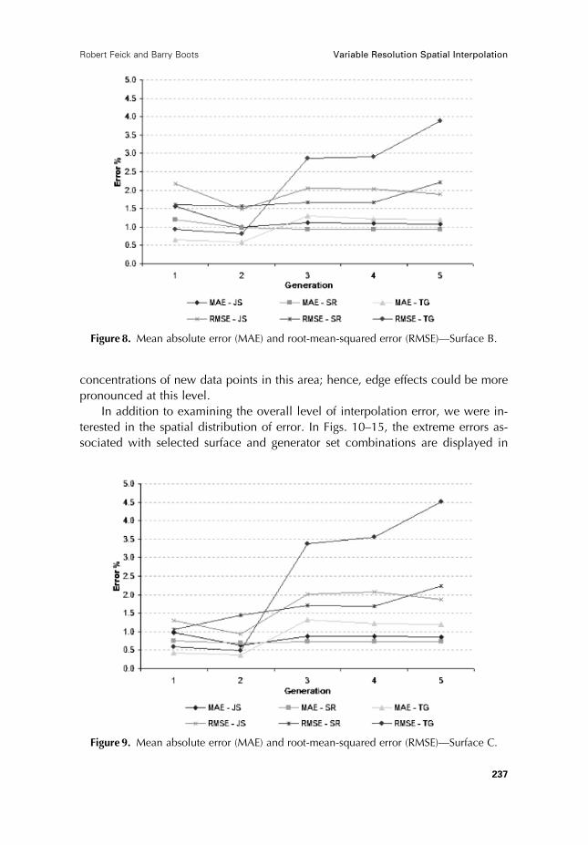
concentrations of new data points in this area; hence, edge effects could be more

pronounced at this level.

In addition to examining the overall level of interpolation error, we were in-

terested in the spatial distribution of error. In Figs. 10–15, the extreme errors as-

sociated with selected surface and generator set combinations are displayed in

Figure 8. Mean absolute error (MAE) and root-mean-squared error (RMSE)—Surface B.

Figure 9. Mean absolute error (MAE) and root-mean-squared error (RMSE)—Surface C.


237

three dimensions (see http://www.fes.uwaterloo.ca/u/rdfeick/index.html for the

complete set of figures). Positive errors (overestimates) are shown as dark-colored

extrusions above the surface in these figures, while negative errors (underestimates)

are shown as light extrusions that extend below the surface. No vertical exagger-

ation was applied to the surfaces; however, the magnitude of the errors was mul-

tiplied by 3 to produce Z-values that could be more easily visualized. For

convenience, Surfaces A–C are shown extending somewhat beyond the convex

hulls associated with the JS, RS, and TG generator sets.

Figs. 10–15 show that negative errors are both more common and generally of

a greater magnitude than positive errors. As underestimation is more evident as

surface complexity increases, we suspect that at least part of this tendency is related

to the generator sets being insufficient in size to capture topographic variations

adequately.

The figures also show that most of the extreme errors are concentrated around

the edges of the convex hulls formed by the initial generator points. This is

particularly apparent for the TG generator set (see Fig. 13) as all of the extreme

errors for all three surfaces are found in proximity to the periphery of the study area.

This suggests that the errors associated with the TG sample are at least partially an

artifact of the original point configuration given that the generators were located on

a nonequilateral triangular grid. The presence of the 15 most pronounced extreme

Figure 10. Surface A extreme errors—jittered square generators.

Figure 11. Surface A extreme errors—stratified random generators.


238

errors does account for the high RMSE values evident for generations 3–5 of the TG

generator set as well.

The ‘‘interior’’ errors in the JS and RS figures show no obvious spatial distri-

bution although there is a tendency for them to be located in small local clusters.

While some of these clusters appear to be associated with initial generator points,

this does not appear to be a general tendency. Indeed, we had anticipated that there

might be a positive relationship between error magnitude at a generated location

and the distance of that location to the nearest initial generator point. However,

with the exception of the 1st generation of some surface and sample design com-

binations, this relationship was not found.

As an example, Fig. 16 shows the situation for Surface A and the JS generator

set. In this figure, the distance of each extreme error point to the nearest generator

point (generation 0) is plotted. Based on the arrangement of the JS generator points,

the furthest a new data point could be from a generator point would be approx-

imately 25,000m. In contrast, the largest concentration of extreme errors occurs at

distances between 7000 and 12,000m.

Discussion and conclusions

The primary aim of this article was to introduce an automated method, based on the

SRPVD, for progressively increasing the density of an initial point set, thus provid-

ing a basis for interpolating surfaces of variable resolution from sparse samples of

Figure 12. Surface B extreme errors—stratified random generators.

Figure 13. Surface B extreme errors—Triangular grid generators.


239

data sites. As we show, an attractive feature of this procedure is that it can be

readily implemented in Arc/Info.

In our illustrative examples, absolute errors in excess of 5 percent of the var-

iable ranges generally occurred at less than 5 percent of the generated data sites.

Clearly, the global error measurements (e.g., MAE, RMSE, extreme error counts)

discussed were affected by the general problem of interpolating data values near a

study area boundary. However, the lack of systematic relationships between error

values and characteristics of either the underlying surface or the initial point set

suggests that the procedure may be robust with respect to these features. Further,

the observation that, after an initial change, the average level of error remains rel-

atively constant may be a desirable feature for those who require a multiresolution

hierarchical data set with little variation in accuracy at different levels. For exam-

ple, in hydrological modelling, one may wish to use a finer spatial resolution for

detailed model runs while maintaining consistency with coarser resolutions used

for cruder models.

However, in order to confirm our initial findings much more testing needs to be

carried out. For example, we need to further explore the sensitivity of the results for

a given surface to different spatial sampling designs for selecting the generator

points and to different sizes of generator point sets. We also need to consider a

range of surfaces with different characteristics, especially more complex surfaces.

Also, of course, we need to compare the performance of the procedure relative to

other COTS interpolation procedures.

Figure 14. Surface C extreme errors—jittered square generators.

Figure 15. Surface C extreme errors—stratified random generators.


240

Notwithstanding the need for further testing, there are several ways the proce-

dure may be refined and extended. For example, it is possible, and probably de-

sirable, not to add all the Voronoi vertices of a given generation to the generator set

for the next generation. In the present context, there are at least two circumstances

where this would be appropriate. First, we may wish to constrain the new gener-

ators to those within a specific distance range of existing generators. If the potential

new generators are very close to existing ones, we can expect that they may add

little new information and thus may be discarded. Similarly, if a potential new

generator is more than some specified distance from an existing generator it may be

unwise to extend interpolation to that generator. One means of identifying such an

upper limit would be to use the characteristics of the semi-variogram of the initial

data points, perhaps limiting new generators to those whose distance to existing

generators is less than half of the range of the semi-variogram. A similar strategy has

been used successfully in the choice of control points in classification of spatial

imagery into classes (Shine and Wakefield 1999) and in two other articles in this

issue (Goovaerts 2005; Kyriakidis and Yoo 2005). We may also wish to relate the

addition of new generators to the nature of local changes in attribute values. While

it is useful to have increased resolution in areas where there are marked changes in

attribute values, little is gained by increasing the resolution in areas where there is

little variation. There has already been some initial consideration of such a gen-

erator constrained recursive point Voronoi diagram (Boots et al. 2002).

Although we illustrated our procedure using quantitative data, it is also appli-

cable to categorical data. In this case, instead of a single value being interpolated at

each generated point, a vector of fuzzy membership values (FMVs) for classes can

be interpolated (Lowell 1994) and equation (1) will need to be adjusted accord-

Figure 16. Surface A extreme errors and generator proximity—jittered square generators.


241

ingly. FMV surfaces can then be generated for each class. Alternatively, at each

recursion, each polygon can be labeled with the value of its generator and these

values mapped to create a piecewise continuous surface (choropleth map).

Acknowledgements

We are grateful for the helpful comments of three anonymous reviewers and

the guest editor, which led to improvements in both the article’s content and

presentation.

References

Boots, B., R. D. Feick, N. Shiode, and S. Roberts. (2002). ‘‘Investigating Recursive Point

Voronoi Diagrams.’’ In Geographic Information Science: Second International

Conference, GIScience 2002, Boulder, CO, USA, September 2002. Lecture Notes in

Computer Science, Vol. 2478: 1–21, edited by M. J. Egenhofer and D. M. Mark. Berlin,

Germany: Springer-Verlag.

Boots, B., and N. Shiode. (2003). ‘‘Recursive Voronoi Diagrams.’’ Environment and Planning

B: Planning and Design 30, 113–24.

Cignoni, P., E. Puppo, and R. Scopigno. (1997). ‘‘Representation and Visualization of Terrain

Surfaces at Variable Resolutions.’’ The Visual Computer 13, 199–217.

De Floriani, L. (1989). ‘‘A Pyramidal Data Structure for Triangle-Based Surface Description.’’

IEEE Computer Graphics and Applications 9, 67–78.

De Floriani, L., B. Falcidieno, and C. Pienovi. (1985). ‘‘Delaunay-Based Representation of

Surfaces Defined over Arbitrarily Shaped Domains.’’ Computer Vision, Graphics, and

Image Processing 32, 127–40.

De Floriani, L., and P. Magillo. (2002). ‘‘Multiresolution Mesh Representation: Models and

Data Structures.’’ In Multiresolution in Geometric Modelling, 363–418, edited by

M. Floater, A. Iske, and E. Quak. Berlin, Germany: Springer-Verlag.

De Floriani, L., P. Magillo, S. Bussi, and E. Bailey. (2000). ‘‘Triangle-Based Surface Models.’’

In Intelligent Systems and Robotics, 340–73, edited by G. W. Zobrist and C. Y. Ho.

Australia: Gordon and Breach Scientific Publishers.

De Floriani, L., P. Marzano, and E. Puppo. (1996). ‘‘Multiresolution Models for Terrain

Surface Description.’’ The Visual Computer 12, 317–46.

De Floriani, L., and E. Puppo. (1992). ‘‘A Hierarchical Triangle-Based Model for Terrain

Description.’’ In Theories and Methods of Spatio-Temporal Reasoning in Geographic

Space. Lecture Notes in Computer Science, Vol. 639: 236–51, edited by A. Frank,

I. Campari, and U. Formentini. Berlin, Germany: Springer-Verlag.

De Floriani, L., and E. Puppo. (1995). ‘‘Hierarchical Triangulation for Multi-Resolution

Surface Description.’’ ACM Transactions on Graphics 14, 363–411.

Garland, M. (1999). ‘‘Multiresolution Modeling: Survey & Future Opportunities.’’

Eurographics ’99, STAR—State of the Art Reports, 111–31.

Goovaerts, P. (2005). ‘‘Exploring Scale-Dependent Correlations Between Cancer Mortality

Rates Using Factorial Kriging and Population Weighted Semivariograms: A Simulation

Study.’’ Geographical Analysis 37, 152–82.


242

Hutchinson, M. F., and J. C. Gallant. (1999). ‘‘Representation of Terrain.’’ In Geographical

Information Systems: Principles, Techniques, Applications, and Management, Vol. 1,

2nd ed. 105–24, edited by P. A. Longley, M. F. Goodchild, D. J. Maguire, and

D. W. Rhind. New York: Wiley.

Klein, R., and W. Stra�er. (1997). ‘‘Generation of Multiresolution Models from CAD Data for

Real Time Rendering.’’ In Theory and Practice of Geometric Modeling (Blaueuren II),

edited by R. Klein, W. Stra�er, and R. Rau. Berlin, Germany: Springer-Verlag.

Kyriakidis, P. C., and E.-H. Yoo. (2005). ‘‘Geostatistical Prediction/Simulation of Point Values

from Areal Data.’’ Geographical Analysis 37, 124–51.

Lowell, K. E. (1994). ‘‘A Fuzzy Surface Cartographic Representation for Forestry Based on

Voronoi Diagram Area Stealing.’’ Canadian Journal of Forest Research 24, 1970–80.

Okabe, A., B. Boots, K. Sugihara, and S. N. Chiu. (2000). Spatial Tessellations: Concepts and

Applications of Voronoi Diagrams, 2nd ed. Chichester, UK: Wiley.

Scallatos, L. L., and T. Pavlidis. (1992). ‘‘Hierarchical Triangulation Using Cartographic

Coherence.’’ CVGIP: Graphical Models and Image Processing 54(2), 147–61.

Shine, J. A., and G. I. Wakefield. (1999). ‘‘A Comparison of Supervised Imagery Classification

Using Analyst-Chosen and Geostatistically-Chosen Training Sets.’’ Geocomputation 99

(CD-ROM).

Sibson, R. (1978). ‘‘Locally Equiangular Triangulations.’’ The Computer Journal 21, 243–45.

Sibson, R. (1981). ‘‘A Brief Description of Natural Neighbour Interpolation.’’ In Interpreting

Multivariate Data, edited by V. Barnett. New York: Wiley.

Voightmann, A., L. Becker, and K. Hinrichs. (1994). ‘‘Hierarchical Surface Representations

Using Constrained DELAUNEY (sic) Triangulations.’’ In Advances in GIS Research:

International Symposium on Spatial Data Handling, Vols 1 & 2: 848–67.

Wang, K., C. P. Lo, G. A. Brook, and H. A. Arabnia. (2001). ‘‘Comparison of Existing

Triangulation Methods for Regularly and Irregularly Spaced Height Fields.’’

International Journal of Geographical Information Science 15, 743–62.

Watson, D. F. (1992). Contouring: A Guide to the Analysis and Display of Spatial Data.

Oxford, UK: Pergamon Press.


243

variable resolution spatial interpolation using the simple recursive point voronoi diagram ·...

Documents