variable returns to agglomeration and the effect of road...

Journal of Urban Economics 62 (2007) 103–120www.elsevier.com/locate/jue

Variable returns to agglomeration and the effectof road traffic congestion

Daniel J. Graham ∗

Centre for Transport Studies, Imperial College London, London SW7 2AZ, UK

Received 22 June 2006; revised 25 October 2006

Available online 20 December 2006

Abstract

This paper investigates the links between returns to urban density, productivity and road traffic conges-tion. A generalised translog production-inverse input demand function is estimated to test for the existenceof variable returns to agglomeration in manufacturing, construction and service industries. Two separatemeasures of urban density, in which proximity is represented by straight line distance or by generalisedcost, are constructed and included in the translog to identify the effect of road traffic congestion. The resultsshow that for some sectors of the economy diminishing returns to urban density can set in causing the mag-nitude of agglomeration elasticity to fall as effective densities increase. The generalised cost based measureof agglomeration produces higher elasticities because it captures both time and distance dimensions of den-sity. A comparison of spatial variance in estimates indicates that road traffic congestion plays an importantrole in explaining diminishing returns for the most highly urbanised locations.© 2006 Elsevier Inc. All rights reserved.

JEL classification: R12; R41

Keywords: Agglomeration; Productivity; Congestion; Translog

1. Introduction

The theoretical foundations for the existence of agglomeration externalities are well estab-lished (see for example Fujita et al. [14], Fujita and Thisse [15], Duranton and Puga [11]). Thereis also now a good deal of empirical evidence on the extent of agglomeration externalities for

* Fax: +44(0)20 7594 6107.E-mail address: [email protected].

0094-1190/$ – see front matter © 2006 Elsevier Inc. All rights reserved.doi:10.1016/j.jue.2006.10.001

104 D.J. Graham / Journal of Urban Economics 62 (2007) 103–120

manufacturing industries. For instance, Ciccone and Hall [6] estimate that average labour pro-ductivity in manufacturing increases by 6% as the employment density of US states doubles;Ciccone [5] reports an elasticity of average labour productivity with respect to employment den-sity of 0.045 for manufacturing in EU regions; and Rice et al. [30] estimate an elasticity ofproductivity with respect to economic mass of 0.035 for UK manufacturing. There are a numberof other studies, stretching back to the early 1970s, which have estimated agglomeration external-ities and have typically reported positive elasticities for manufacturing industries of somewherebetween 2% and 10% (for reviews see Rosenthal and Strange [31], Eberts and McMillen [13]).

Despite this evidence, we also know that there are limits to urban growth and that cities canexperience declines in population, employment and even output. A number of empirical studieshave found evidence of centrifugal forces that can induce industrial dispersion from cities andhave also indicated the existence of agglomeration diseconomies (e.g. Beeson [1,2], Carlino [4],Moomaw [27], Hansen [18], Hanson [19]). Urban economic theory does, of course, allow fordisparities in the nature of returns to agglomeration and also recognises that for many types ofeconomic activity a highly urbanised location may not be optimal. The new economic geographyliterature has illustrated these themes by focusing on the interaction between increasing returns,wages and the costs of trade (e.g. Fujita et al. [14], Fujita and Thisse [15]).

Theory tells us that the strength of centripetal forces can be limited or diminished as cities be-come too large and the processes which give rise to positive externalities consequently becomeless efficient. Prominent amongst the inefficiencies mentioned in this respect is the existenceof congestion in urban transport systems. There is an inherent tendency for externalities of ag-glomeration and congestion to coincide spatially; the former are thought to be derived fromconcentration and the latter are a consequence of it. In other words, we expect congestion to bepresent in those locations where the competition in factor input and output markets is intense(see Coombes and Overman [7]). There, is therefore a very close relationship between urbancongestion and agglomeration economies. For this reason, it may be informative to consider theextent to which the benefits of urban density, generated through agglomeration externalities, areconstrained by road traffic congestion.

In this paper we provide an empirical investigation of the effect of urban congestion on ag-glomeration.1 Our main focus is on determining whether we can identify variable returns fromagglomeration and whether any such externalities may be constrained by congestion in cities.The paper estimates nonlinear agglomeration elasticities in a generalised translog productionfunction to test for the existence of variable returns. Effective density based measures of agglom-eration are constructed to capture the scale and proximity of activity that is accessible to anylocation. Proximity is represented in two different ways: by distance and by the generalised costof road travel which includes information both about distances and road speeds. Comparing re-sults using densities based on each measure of proximity we are able to investigate the impactof congestion on returns to agglomeration. Results are presented for manufacturing, constructionand for seven service sectors: distribution, hotels & catering; transport, storage & communica-tions; real estate; information technology; banking, finance & insurance; business services; andpublic services (see Appendix A for a description of these sectors).

1 Note that we are concerned in this paper with the relationship between economic productivity and the concentra-tion of industry per se, regardless of the mix of intra-industry and inter-industry densities. Studies that have set out todistinguish the productivity effects of urbanisation and localisation within the same model include Nakamura [28], Hen-derson [22], Henderson [23] and Graham [16]. Recent studies of localisation are provided by Duranton and Overman [12]and Devereaux et al. [8].

D.J. Graham / Journal of Urban Economics 62 (2007) 103–120 105

The paper is structured as follows. Section 2 describes the translog production-inverse in-put demand function which we use as a basic framework for the estimation of agglomerationexternalities. Section 3 describes data sources and explains the measures of agglomeration thatwe construct and how we use these to shed light on the effect of urban road traffic congestion.Empirical results are presented in Section 4 and conclusions are drawn in the final section.

2. The translog production-inverse input demand function

We analyse the relationship between productivity and agglomeration within a productionfunction framework. The translog inverse input demand function proposed by Kim [24,25]provides a very flexible functional form for estimation which allows for a non-homothetic pro-duction technology with variable returns to scale (RTS). Agglomeration can be estimated asa Hick’s neutral production function shifter and the quadratic form allows this elasticity to varyacross the sample with the level of agglomeration.

The translog approximation to a firm level production function is

logY = α0 + βU logU + 1

2βUU(logU)2 +

n∑i=1

αi logXi

+ 1

2

n∑i=1

n∑j=1

γij logXi logXj (1)

where Y is the output level of the firm, X is a vector of factor inputs with elements Xi

(i = 1, . . . , n), and U is some measure of the level of agglomeration experienced by the firm.The firm faces an expenditure constraint in which input prices (Wi ) and quantities determine

total cost (C):∑i

WiXi = C. (2)

Given competitive inputs markets the maximisation of output subject to the expenditure con-straint implies that

∂Y

∂Xi

= λWi, (3)

where λ is a Lagrange multiplier which is the reciprocal of marginal cost ∂C/∂Y .From (2) and (3)

λ =∑

i (∂Y/∂Xi)Xi

C(4)

and substituting (4) back into (3) after rearrangement yields the inverse input demand equations

Wi

C= ∂Y/∂Xi∑

i (∂Y/∂Xi)Xi

. (5)

The inverse input demand functions determine prices as functions of quantities as opposed toordinary demand functions which determine quantities in terms of prices.

Equation (5) can be written in cost share form (SCi ) as

SCi = WiXi

C= ∂ logY/∂ logXi∑

∂ logY/∂ logX, (6)

i i


and therefore differentiation of (1) can be used to obtain the cost share equations

SCi = αi + ∑

j γij logXj∑i αi + ∑

i

∑j γij logXj

. (7)

The translog parameters can be efficiently estimated by simultaneously estimating (1) and (7)as a nonlinear multivariate regression system. The generalised translog function provides a flex-ible framework for estimation in which the level of returns to scale can vary across the sampledepending on the level of production. Homotheticity and homogeneity represent restricted ver-sion of the production technology allowed by Eq. (1).2 It is desirable that we adopt a flexiblefunctional form for estimation if we wish to be effective in isolating the impact of agglomera-tion across the sample. Use of more restrictive functional forms, for instance one that estimatesa constant level of RTS, can give rise to a less adequate fit and consequently yield less efficientestimates.

Returns to agglomeration are expressed in a quadratic relationship. The effect of agglomera-tion on production at each point on this quadratic curve can be measured by

∂ logY

∂ logU= βu + βUU logU. (8)

Equation (8) measures the total shift in output that arises from agglomeration. Since we havecontrolled for input use and the effect of RTS within the production function, the output shiftshown in (8) is also a shift in total factor productivity (TFP). Note that non-linear agglomerationeffects are accommodated by this elasticity which varies depending on the level of agglomeration.The quadratic specification allows for variable returns including the kind of diminishing returnsthat might be predicted by theory.

3. Estimating agglomeration and the effect of congestion

To estimate the translog system we need data with detailed geographical and sectoral dis-aggregation. The data we have found that match these requirements are the firm level data ofregistered UK companies. Under UK legislation each registered company is required to provideaccounting and other data about their operations to an executive agency of the Department ofTrade and Industry know as Companies House. These data are made available in a commercialsoftware package called Financial Analysis Made Easy (FAME), which is produced jointly byJordans and Bureau Van Dijk (BVD [3]).

FAME record extensive financial data for each company including turnover, a breakdown ofcosts, and information on the number of employees and on the total assets held by the firms. Weuse turnover as a measure of output, the number of employees as labour input, and we calculateaverage wages per employee from total payroll. As a proxy for capital input we use informationon total assets. This includes the value of include ‘fixed assets’ such as the buildings, plant,machinery and equipment and ‘current assets’ such as stocks and various debts owed by and tothe company. We treat total assets as a proxy for capital input (K) in the sense that they givea measure of the value of the non-labour inputs available.

2 A homothetic and homogeneous technology is imposed by the restriction∑

j γij = 0. Graham and Kim [17] estimatea non-homothetic version of this generalised translog function allowing for factor augmenting agglomeration effects.They show that this model specification can be used to analyse the effect of agglomeration on partial factor productivity,total factor productivity, factor prices and factor demands.


FAME also records information about the location of the company. Since the data are providedby companies and not plants they can include firms that have plants in many locations but thatonly report aggregated records. To isolate single plants firms from the FAME data we have takenthe following steps. First, we have removed firms that record more than one UK trading address.Second, we have removed firms that have a registered office address that is different from theirmain trading address. Third, we have kept only those firms that do not have a UK or foreignholding or subsidiary company. Fourth, as a further precaution, we have removed large firmsfrom the data because these could record all of their information from one UK registered officeaddress, typically their headquarters, but not provide information about other plants they mayhave located in different areas of the UK or the World. Our sample is based on firms that haveless than 100 employees.

The FAME data are available for a number of years, although the quantity and quality of thedata diminishes as we go back in time. We have extracted FAME data over the period 1995 to2002 for 9 industry groups (see Appendix A).

The principal concern in this paper is with the impact of urban congestion on the relationshipbetween productivity and agglomeration. As discussed above, we can estimate the translog witha measure of agglomeration expressed in quadratic from to identify if there are diminishingreturns. However, the presence of diminishing returns itself does not verify the existence of urbancongestion. There could be a number of reasons why cities become less efficient as size grows. Toidentify the impact of urban transport congestion we need to construct measures of agglomerationthat contain an implicit transport dimension and that allow us to consider the implications ofconstraints on the efficiency of travel.

Thus, crucial to our measures of agglomeration is some quantification of the relative ease ofaccessing urban activity. In other words, we are not just interested in city size or scale but alsoin the relative proximity of activities, spatially and temporally. This leads naturally to a consid-eration of densities and in this paper we base our analysis of agglomeration on the concept ofeffective densities. An effective density measures the amount of ‘activity’ that is accessible fromsome given location.

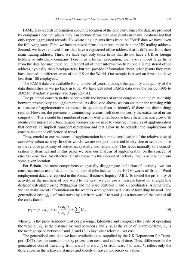
For Britain, the most comprehensive spatially disaggregate definition of ‘activity’ we canconstruct makes use of data on the number of jobs located in the 10,780 wards of Britain. Wardemployment data are reported in the Annual Business Inquiry (ABI). To model the proximity ofactivity, or the nearness of one ward to the next, we can use a measure based on straight linedistance calculated using Pythagoras and the ward centroid x and y coordinates. Alternatively,we can make use of information on the ward to ward generalised costs of travelling by road. Thegeneralised cost (gij ) of road travel by car from ward i to ward j is a measure of the total of allthe costs faced:

gij = p · rdij + τv

(rdij

sij

)+

∑c

Uc, (9)

where p is the price or money cost per passenger kilometre and comprises the costs of operatingthe vehicle, rdij is the distance by road between i and j , τv is the value of in vehicle time, sij isthe average speed between i and j , and Uc is any other relevant user cost.

The generalised cost data we have available to us, supplied by the UK Department for Trans-port (DfT), assume constant money prices, user costs and values of time. Thus, differences in thegeneralised cost of travelling from ward i to ward j , or from ward i to ward k, reflect only thedifferences in the relative distances and speeds of travel, not prices or values.


Using these measures of proximity we can define two effective density measures for a firm inindustry o located in ward i as follows

UDio = Ei

ri+

i �=j∑j

(Ej

dij

), (10)

UGio = Ei

gi

+i �=j∑j

(Ej

gij

)(11)

where E is total employment, ri is an approximation of the radius of ward i,3 and dij is theEuclidean distance between i and j . The effective density measures closely resemble the conceptof market potential developed by Harris [21] and used in recent empirical work by Mion [26] andHanson [20].

Comparing the values of UD and UG should enable us to investigate urban road traffic con-gestion because the essential difference between the two lies in the inclusion, or exclusion, orinformation about the speed of travel. Our hypotheses are as follows. In large cities, where con-gestion is present, the ratio of UD to UG will tend to be relatively large because while there isa lot of activity concentrated in space, road traffic speeds are low and so the generalised costof travelling small distances is high. In smaller towns and cities where there is less congestionand consequently higher road speeds the ratio of UD to UG will less. In rural areas where trafficmoves at free flowing speeds we will expect the ratio of UD to UG to be at a minimum.

Essentially, we are hypothesising that if congestion exists then these two measures will tendto diverge as we move towards the upper end of the urban hierarchy. The generalised cost basedmeasure of proximity accounts for the fact that speeds can vary systematically with city size andthis provide a sort of upper constraint on the values of urbanisation. The absence of informationabout travel times or speeds in the UD variable induces an artificial right-hand skew into thedistribution of urbanisation values: it makes locations that suffer from congestion seem moreaccessible than they really are. In this sense we can argue that if congestion exists, the UDvariable will contain some degree of measurement error.

If it is true that the generalised cost based density variable provides a superior measure ofthe actual level of agglomeration experienced by firms, then it follows that estimation usinga measure based on Euclidean distance will produce a biased estimate of the agglomerationelasticity. We can demonstrate this in the following way. Let the estimating equation for (1)based on the generalised cost (UG) measure of agglomeration be written in shorthand form as

Y = α + βuUG +∑

i

βiXi + u (12)

where the logarithmic and quadratic forms of the variables have been suppressed. We assume thisto be the ‘true’ model with agglomeration measured to a reasonable degree of accuracy by UG. Ifinstead of estimating (12) we estimate using the variable UD which contains measurement errorwe have

Y = α + βuUD +∑

i

βiXi + v

= α + βuUD +∑

i

βiXi + βu(UG − UD) + u (13)

3 This ‘radius’ is approximated from the ward area as√

area /π .
i


where the error term v in the first row of (13) can be decomposed into two components: theterm βu(UG − UD) and the error u from the true model. Since UD will be correlated with thisfirst component of the error term, the estimate of βu obtained from (13) will be biased, with thedirection of the bias depending on the correlation between UD and (UG − UD). In the presenceof congestion, we expect speeds to fall and therefore generalised costs to grow as the level of thevariable UD increases, and so the UG variable should grow less than proportionately with UD.Therefore, if congestion does exist UD should be negatively correlated with (UG − UD) andconsequently the estimates of the agglomeration elasticity based on UD should be downwardsbiased.

4. Results

The results section is organised as follows. First, we present results from estimation of a twofactor non-homothetic translog system

logY = α0 + βt t + βU logU + 1

2βUU(logU)2 + βL logL + βK logK

+ 1

2γLL(logL)2 + 1

2γKK(logK)2 + γLK logL logK,

SL = βL + γLL logL + γLK logK

βL + βK + (γLL + γLK) logL + (γKK + γLK) logK. (14)

We estimate (14) separately using two effective density measures of agglomeration. First, weuse the more conventional measure of agglomeration with proximity based on distance (UD)to test for the existence of agglomeration externalities in different sectors of the economy andto identify any evidence of diminishing returns. Second, we estimate using the generalised cost(UG) based agglomeration variable and then compare results. If congestion does exist, we wouldexpect elasticity estimates based on UG to be higher than those based on UD and we may alsoexpect to find differences in the estimates that capture the extent of diminishing returns.

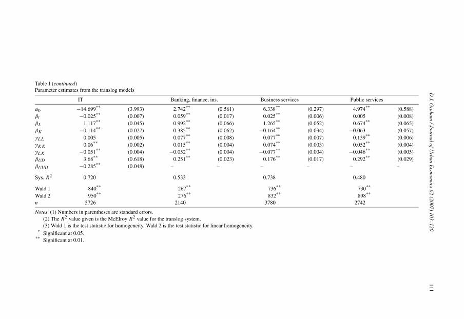
Table 1 shows results of the estimation of Eq. (14) using the UD variable for our nine industrygroups. The Wald statistics associated with each regression allow us to reject the hypothesis thathomogeneity or linear homogeneity can provide a superior characterisation of the structure ofproduction. Production function parameter estimates are, with few exceptions, significant andof the expected sign. Results relating to the structure of production are summarised in Table 2,calculated at the sample means.

Estimates of RTS from the translog models indicate that firms within our industry groups tendto operate reasonably near constant returns to scale. For manufacturing, the output elasticity oflabour is 0.27 and is under half the size of the capital output elasticity. Services tend to be morelabour intensive and this is reflected in the output elasticities of labour around or above 0.45 inbanking and finance, IT services, business services, and public services.

Our main concern in this paper is on the estimates associated with the agglomeration variables(βUD and βUUD). The quadratic form for agglomeration produced significant estimates for five ofthe nine industries shown in Table 1. For the remaining four industries, we estimated insignificantquadratic coefficients and found that a log-linear relationship between output and agglomerationproduced a better fit. Table 3 summarises the evidence on agglomeration externalities showing,for each industry group, the relevant parameter estimates from the translog and the elasticities ofoutput with respect to agglomeration. Where the quadratic form has been used these elasticitiesare evaluated using the mean level of agglomeration of each sample.

110D

.J.Graham

/JournalofUrban

Econom

ics62

(2007)103–120

ans., store, & comm. Real estate

.234 (4.748) 5.251** (0.583)

.003 (0.006) 0.001 (0.007)

.938** (0.034) 1.044**

.673** (0.038) 0.052 (0.072)

.066** (0.003) 0.091** (0.010)

.009** (0.003) 0.051** (0.005)

.064** (0.002) −0.055** (0.005)

.48* (0.732) 0.084** (0.024)

.095 (0.057) – –

.536 0.501

749** 260**

778** 261**

4411 3947

Table 1Parameter estimates from the translog models

Manufacturing Construction Dist., hotels & cater.

α0 −1.403 (1.802) −24.849** (4.874) −9.602** (2.306) −βτ −0.001 (0.002) 0.037** (0.012) −0.091** (0.004)

βL 1.124** (0.018) 0.852** (0.047) 0.731** (0.022)

βK 0.26** (0.016) 0.31** (0.070) 0.178** (0.036)

γLL 0.074** (0.002) 0.075** (0.005) 0.063** (0.002)

γKK 0.047** (0.001) 0.039** (0.005) 0.055** (0.003)

γLK −0.076** (0.001) −0.062** (0.003) −0.052** (0.002) −βUD 1.105** (0.283) 4.79** (0.776) 2.488** (0.355)

βUUD −0.086** (0.022) −0.369** (0.062) −0.188** (0.028) −Sys. R2 0.676 0.539 0.609

Wald 1 5624** 566** 2452**

Wald 2 5626** 566** 2605**

n 13,003 3139 9658

Tr

700000010

0

D.J.G

raham/JournalofU

rbanE

conomics

62(2007)

103–120111

s Public services

(0.297) 4.974** (0.588)

(0.006) 0.005 (0.008)

(0.052) 0.674** (0.065)

(0.034) −0.063 (0.057)

(0.007) 0.139** (0.006)

(0.003) 0.052** (0.004)

(0.004) −0.046** (0.005)

(0.017) 0.292** (0.029)

– – –

0.480

730**

898**

2742

Table 1 (continued)Parameter estimates from the translog models

IT Banking, finance, ins. Business service

α0 −14.699** (3.993) 2.742** (0.561) 6.338**

βt −0.025** (0.007) 0.059** (0.017) 0.025**

βL 1.117** (0.045) 0.992** (0.066) 1.265**

βK −0.114** (0.027) 0.385** (0.062) −0.164**

γLL 0.005 (0.005) 0.077** (0.008) 0.077**

γKK 0.06** (0.002) 0.015** (0.004) 0.074**

γLK −0.051** (0.004) −0.052** (0.004) −0.077**

βUD 3.68** (0.618) 0.251** (0.023) 0.176**

βUUD −0.285** (0.048) – – –

Sys. R2 0.720 0.533 0.738

Wald 1 840** 267** 736**

Wald 2 950** 276** 832**

n 5726 2140 3780

Notes. (1) Numbers in parentheses are standard errors.(2) The R2 value given is the McElroy R2 value for the translog system.(3) Wald 1 is the test statistic for homogeneity, Wald 2 is the test statistic for linear homogeneity.

* Significant at 0.05.** Significant at 0.01.


Table 2Estimated returns to scale and output elasticities calculated using sample means of the data

RTS Output elasticities

labour capital

Manufacturing 0.956 0.274 0.682Construction 0.878 0.200 0.678Distributions, hotels & catering 0.976 0.176 0.800Transport, storage & communications 0.862 0.232 0.630Real estate 1.096 0.398 0.699IT 1.030 0.505 0.525Banking, finance & insurance 0.912 0.445 0.467Business services 1.063 0.452 0.611Public services 0.932 0.442 0.491

Table 3Elasticities of output with respect to agglomeration (UD variable)

βUD βUUD εUD

Manufacturing 1.105** −0.086** 0.041Construction 4.79** −0.369** 0.214Distrib., hotels & catering 2.488** −0.188** 0.133Trans., storage & comm. 1.48* −0.095 0.274Real estate 0.084** – 0.084IT 3.68** −0.285** 0.089Banking, fin. & insurance 0.251** – 0.251Business services 0.176** – 0.176Public services 0.292** – 0.292


We estimate positive agglomeration externalities for manufacturing, construction and for eachof our seven service industries. The lowest agglomeration elasticity shown in the table is formanufacturing, 0.041. This measures up reasonably well to roughly comparable estimates of0.06 for the US states (Ciccone and Hall [6]), 0.045 for EU regions (Ciccone [5]), and 0.035for UK manufacturing (Rice et al. [30]). The largest agglomeration elasticities are for transportstorage & communications (0.274),4 construction (0.214), banking finance & insurance (0.251),business services (0.176), and public services (0.292). The average for the seven service sectors is0.186, over four times larger in magnitude than for manufacturing. So it seems, on the basis of thefigures given in Table 3 that services enjoy higher returns from agglomeration than manufacturingand particularly the types of activities that we expect to find in CBD locations such as bankingfinance & insurance, and business services.

Table 3 also provides some evidence about the existence of variable returns. We estimatenegative and significant quadratic parameters (βUUD) for five sectors. For the remaining four in-dustries we find insignificant quadratic terms but achieve a good fit with a single parameter for

4 For transport providing firms, the higher elasticities may be indicative of the increasing returns to density which tendto affect transport operators such that unit costs fall as the density of traffic increases. Passenger densities are likely togrow systematically with city size.


the sample as a whole indicating that returns to agglomeration are constant. Figure 1 illustratesthe nature of the five quadratic relationships we have estimated by evaluating the agglomera-tion elasticities for each ward of Britain using the ward agglomeration values.5 Note that theelasticities vary at each point in the sample and so the plots show the marginal relationship be-tween productivity and agglomeration. Thus, where the elasticities are greater than zero thereare increasing returns to agglomeration, where they equal to zero returns to agglomeration aremaximised, and where they are less than zero returns are decreasing.

Each of the five sectors shown in Fig. 1 exhibits some degree of diminishing returns to ur-ban density. For manufacturing, IT and construction, returns to agglomeration are maximised(elasticity = 0) at around the same point. In fact, although this looks to be at a relatively lowvalue of agglomeration the distribution has a right-hand skew and for these three industries weactually find positive but diminishing returns over the first nine deciles of agglomeration values.The distribution hotels & catering industry reaches a maximum value of returns to agglomerationslightly later and then decreasing returns thereafter in a small proportion of the most highly ur-banised wards. For transport storage & communications we have evidence of diminishing returnsbut the quadratic function is not maximised using this sample and we do not identify decreasingreturns to agglomeration.

To shed light on the impact of road traffic congestion we next introduce the effective densitymeasure based on generalised cost. Re-estimating the translog using the UG variable we generatea new set of agglomeration elasticities which we denote εUG. These are shown in Table 4 andcompared in Fig. 2 to the elasticities obtained using effective density measures based on distance.The results of the estimation relating to the structure of production are very similar to thosepresented in Tables 1 and 2 and so we do not repeat them here.

The overall pattern of agglomeration estimates obtained using each effective density measureis very similar (Fig. 2). Positive and significant agglomeration economies are estimated for allindustries shown in the table. However, there are two notable differences between the estimatesobtained using the UD or UG variables. First, is that with the exception of elasticity estimates formanufacturing and IT, which are very similar in magnitude, the generalised cost based estimatestends to be higher than the elasticities estimated using distance based measures. Second, usingthe UG variable we find positive and statistically significant quadratic terms (βUUG) for threeservice industries: banking finance & insurance, business services, and public services.

From the comparison of estimates we can make two observations relevant to the impact ofroad traffic congestion on agglomeration externalities. First, as hypothesised in Section 3, wefind that the inclusion of travel time information in the measure of effective density produceshigher estimates of agglomeration externalities. If we believe that generalised cost densities pro-vide a superior measure of agglomeration in the presence of road traffic congestion, then theimplication is that the estimates based on a Euclidean distance measure of density (βUD) aredownward biased. We can confirm the direction of this bias by calculating the correlation be-tween log UD and the term (log UG − log UD) (see Eq. (13)).

Table 5 shows negative correlations for all industries and therefore that the UG measure ofagglomeration grows a slower rate than UD. In other words, the two measures diverge as thelevel of urbanisation increases, with the UD variable yielding more extreme high values. Thisdivergence can induce differences of fairly large magnitude in the UD and UG agglomeration

5 In making these calculations we assume that the parameters estimates obtained from our samples are applicable overthe distribution of all wards.


Fig.

1.Sp

atia

lvar

ianc

ein

retu

rns

toag

glom

erat

ion.

D.J.G

raham/JournalofU

rbanE

conomics

62(2007)

103–120115

neralised cost (εUG).
Fig. 2. A comparison of effective density elasticities based on distance (εUD) and ge


Table 4Elasticities of output with respect to agglomeration (UG variable)

βUG βUUG εUG

Manufacturing 1.265* −0.091* 0.042Construction 3.379* −0.233* 0.243Distrib., hotels & catering 3.096** −0.217** 0.151Trans., storage & comm. 0.35** – 0.350Real estate 0.114** – 0.114IT 6.175** −0.446** 0.082Banking, fin. & insurance −3.449* 0.276* 0.329Business services −1.562* 0.13* 0.226Public services −3.02* 0.252* 0.399


elasticity estimates, particularly for the industries that tend to be most urbanised. For example,the UG estimates are over 30% higher than the UD estimates for real estate, banking finance &insurance, and public services; and are just under 30% higher for business services and transportstorage & communications.

The second observation to be made from the comparison of the agglomeration elasticities isthat evidence on the nature of diminishing returns differs depending on which measure is used.The elasticities based on straight line distance show evidence of diminishing returns for five ofthe nine industry groups and constant returns for the remaining four. The elasticities based on theUG variable, on the other hand, show diminishing returns for only four industry groups, constantreturns for two, and increasing returns for the remaining three.

These two observations offer evidence consistent with the hypothesis that urban road trafficcongestion plays a significant role in ‘constraining’ the benefits of agglomeration, and conse-quently, that it may serve to reduce achievable levels of urban productivity. The generalised costbased measures of proximity accounts for the fact that speeds can vary systematically with citysize. Accordingly, estimates based on UG capture the combined effects of changes in both thedistance and speed dimensions of effective density. The UD measure captures changes in spatialbut not temporal accessibility giving rise to higher extreme values of urbanisation at the upperbound of the distribution. The fact that the gap between the two measures increases as the levelof urbanisation grows, due to the exclusion of travel time information, reflects the impact of roadtraffic congestion.

If, as our empirical analysis suggests, congestion can contribute to the diminishing returns weobserve then the implication is that the productivity benefits of agglomeration could be increasedby making appropriate transport interventions. In other words, the fact that the distance baseddensity elasticities may be smaller in the most urbanised locations does not necessarily imply thatthere cannot be any further advantages from improving accessibility. Rather, our results suggestthat an exogenous intervention to reduce the negative externality of congestion could mitigatethe effects of diminishing returns: it could shift the productivity-urbanisation curve outwards.Venables [32] provides a theoretical example of this type of relationship showing how a reductionin travel times within a city can induce agglomeration benefits.

We can provide a brief demonstration of these issues here by considering a numerical exampleof the effect of changing densities. Table 6 shows elasticities averaged for the London agglom-eration evaluated using the parameters given in Table 4 and the generalised cost agglomeration


Table 5Correlation (r) between log UD and (log UG − log UD)

r

Manufacturing −0.814Construction −0.784Distribution, hotels & catering −0.876Trans., storage & communications −0.884Real estate −0.881IT −0.858Banking, fin. & insurance −0.901Business services −0.892Public services −0.865

Table 6Agglomeration elasticities for the London conurbation, UG variable

εUG Emp. share (%)

Manufacturing 0.00 6Construction 0.12 4Distribution, hotels & catering 0.05 25Transport, storage & communications 0.35 10Real estate 0.11 3IT −0.08 3Banking, finance & insurance 0.41 10Business services 0.27 13Public services 0.51 26

Total weighted average 0.26

values for the London wards. The table also shows a breakdown of the broad industrial structureof London expressed in employment shares. Weighting the elasticities according to these shareswe calculate a total weighted average agglomeration elasticity for all sectors of 0.26.

The London conurbation contains a large volume of employment within a relatively small area(approximately 4 million jobs within 1579 square kilometres). However, many London locationssuffer from congestion and speeds can be low, so the generalised cost of travelling one kilometrewithin London is relatively high with the travel time component comprising around 80% of thetotal.6

If the volume of employment within London, that is the total number of jobs within the GreaterLondon area, was to increase by 5% then on the basis of the sectoral elasticities and shares givenabove we would expect a 1.3% increase in productivity, ceteris paribus. In fact, this scenariowould actually involve a substantial increase of approximately 200,000 jobs within London andwe would therefore expect additional second or third round effects on travel demand, which wecannot predict here, but which would potentially impact on the generalised cost of travel andreduce the net productivity effect.

6 For instance, evaluating the average generalised cost of travelling one kilometre by car in London using parametervalues from DfT [9], appropriate price indices (ONS [29]), and assuming an average speed of 27 kilometres per hour(DfT [10]) gives a value of approximately £0.65 in 2005 prices. Of this total figure, 80% comprises the time component,12% the fuel cost, and the remaining 8% the vehicle operating costs.


If, on the other hand, the volume of employment within greater London was to remain con-stant but travel times were to fall uniformly by five percent, then assuming an 80% share forthe time component of generalised cost, this would give rise to a 4% increase in average UGdensities, and given the elasticities and sectoral share shown in Table 6, we would expect a 1.0%increase in productivity, ceteris paribus. Of course, any such improvement in speeds would notbe costless and would almost certainly require major capacity expansion to the existing networkor the imposition of some comprehensive congestion charging scheme.

These two brief examples are used simply to emphasise that the densities associated withagglomeration have temporal and cost dimensions as well as a physical dimension. The use ofeffective densities based on distance and generalised cost has provided an interesting empiricalperspective on the role that road traffic congestion can play in constraining accessibility. Ofcourse, one crucial assumption we have adopted is that the exclusion of travel time informationin the UD variable introduces measurement error because it make the most highly urbanisedlocations appear more dense than they really are, certainly in temporal terms. This assumptionseems to be supported by our data. However, since not all travel is made by roads, and sincea high proportion of travel by urban rail is common in many cities, the effective density of activitycould actually be higher than represented by road based proximity. Consequently, it is importantto stress that the extent to which error exists in any physical density measure of agglomerationwill depend on the particular travel characteristics of the area under consideration.

5. Conclusions

In this paper we have developed an analysis of agglomeration externalities within the frame-work of a translog production inverse input demand function to test for diminishing return fromurban transport congestion. We have constructed two effective density measures of agglomera-tion that incorporate an explicit transport dimension with proximity modelled using straight linedistances or the generalised costs of road travel. Through comparison, these two measures, andestimates based upon them, can help us identify the impact of road traffic congestion.

The results show that there are diminishing and even decreasing returns to agglomeration forsome sectors of the economy. However, for the types of activity we expect to find in CBDs andlarge urban areas; such as real estate, banking & finance, business services, and public services;our estimates show returns to agglomeration that are constant or increasing. There is greatervariance in the effective density variable when calculated using straight line distances rather thangeneralised costs because the inclusion of information about travel times constrains the values atthe top of the distribution. Use of the generalised costs effective density variable in the translogmodel produces higher agglomeration elasticities and shows less evidence of diminishing returnsbecause it captures both time and distance dimensions of effective density. Put another way, roadtraffic congestion serves to reduce the densities of the most urbanised locations. Consequently, itcan constrain agglomeration externalities and prove an important factor in the diminishing returnto agglomeration that we observe.

Acknowledgments

I would like to thank H. Youn Kim, Lars Rognlien, Gilles Duranton, two anonymous referees,and the journal editor for comments on a previous draft of this paper.


Appendix A. Industry sectors used for estimation

The firm level data are aggregated according to the 1992 SIC in the following ways:

(i) manufacturing (MAN) (SIC 15-40),(ii) construction (CON) (SIC 45),

(iii) distribution, hotels & catering (DHC) (SIC 50-55),(vi) transport, storage & communications (TSC) (SIC 60-64),(v) Real estate (RE) (SIC 70),

(vi) Information technology (SIC 72),(vii) banking, finance & insurance (BFI) (SIC 65-67),

(viii) business services (BUS) (SIC 741-745),(ix) public services (PSE) (SIC 75-90).

References

[1] P.E. Beeson, Total factor productivity growth and agglomeration economies in manufacturing 1959–73, Journal ofRegional Science 27 (2) (1987) 183–198.

[2] P.E. Beeson, Sources of the decline in manufacturing in large metropolitan areas, Journal of Urban Economics 28 (1)(1990) 71–86.

[3] BVD, FAME, UK and Irish company information in an instant, Bureau van Dijk, London, 2003.[4] G.A. Carlino, Declining city productivity and the growth of rural regions: A test of alternative explanations, Journal

of Urban Economics 18 (1) (1990) 11–27.[5] A. Ciccone, Agglomeration effects in Europe, European Economic Review 46 (2) (2002) 213–227.[6] A. Ciccone, R.E. Hall, Productivity and the density of economic activity, American Economic Review 86 (1) (1996)

54–70.[7] P. Coombes, H.G. Overman, The spatial distribution of economic activities in the European Union, in: J.V. Hen-

derson, J.F. Thisse (Eds.), Handbook of Regional and Urban Economics, vol. 4, North-Holland, Amsterdam, 2004,pp. 2845–2909.

[8] M. Devereux, R. Griffith, H. Simpson, The geographic distribution of production activity in the UK, RegionalScience and Urban Economics 34 (5) (2004) 533–564.

[9] DfT, Transport Economics Note, HMSO, London, 2001.[10] DfT, Transport Statistics for Great Britain, HMSO, London, 2005.[11] G. Duranton, D. Puga, Microfoundations of urban agglomeration economies, in: J.V. Henderson, J.F. Thisse (Eds.),

Handbook of Regional and Urban Economics, vol. 4, North-Holland, Amsterdam, 2004, pp. 2063–2117.[12] G. Duranton, H. Overman, Testing for localization using micro geographic data, Review of Economic Studies 72 (4)

(2005) 1077–1106.[13] R.W. Eberts, D.P. McMillen, Agglomeration economies and urban public infrastructure, in: P. Cheshire, E.S. Mills

(Eds.), Handbook of Regional and Urban Economics, vol. 3, North-Holland, Amsterdam, 1999, pp. 1455–1495.[14] M. Fujita, P. Krugman, A.J. Venables, The Spatial Economy: Cities, Regions and International Trade, MIT Press,

Cambridge, MA, 1999.[15] M. Fujita, J. Thisse, The Economics of Agglomeration: Cities, Industrial Location and Regional Growth, Cambridge

Univ. Press, Cambridge, 2002.[16] D.J. Graham, Identifying localization and urbanisation externalities for manufacturing and service industries, Work-

ing paper, Imperial College London, 2006.[17] D.J. Graham, H.Y. Kim, An empirical analytical framework for agglomeration economies, Working paper, Imperial

College London, 2006.[18] E.R. Hansen, Agglomeration economies and industrial decentralization: The wage-productivity trade-off, Journal

of Urban Economics 28 (2) (1990) 140–159.[19] G.H. Hanson, Agglomeration, dispersion and the pioneer firm, Journal of Urban Economics 39 (3) (1996) 255–281.[20] G.H. Hanson, Market potential, increasing returns and geographic concentration, Journal of International Eco-

nomics 67 (1) (2005) 1–24.[21] C.D. Harris, The market as a factor in the localization of industry in the United States, Annals of the Association of

American Geographers 44 (4) (1954) 315–348.


[22] J.V. Henderson, Efficiency of resource usage and city size, Journal of Urban Economics 19 (1) (1986) 47–70.[23] J.V. Henderson, Marshall’s scale economies, Journal of Urban Economics 53 (1) (2003) 1–28.[24] H.Y. Kim, The translog production function and variable returns to scale, Review of Economics and Statistics 74 (3)

(1992) 546–552.[25] H.Y. Kim, The Antonelli versus Hicks elasticity of complementarity and inverse input demand systems, Australian

Economic Papers 39 (2) (2000) 245–261.[26] G. Mion, Spatial externalities and empirical analysis: The case of Italy, Journal of Urban Economics 56 (1) (2004)

97–118.[27] R.L. Moomaw, Firm location and city size: Reduced productivity advantages as a factor in the decline of manufac-

turing in urban areas, Journal of Urban Economics 17 (1) (1985) 73–89.[28] R. Nakamura, Agglomeration economies in urban manufacturing industries: A case of Japanese cities, Journal of

Urban Economics 17 (1) (1985) 108–124.[29] ONS, Retail Price Indices, HMSO, London, 2006.[30] P. Rice, A.J. Venables, E. Patacchini, Spatial determinants of productivity: Analysis for the regions of Great Britain,

Mimeo, London School of Economics, 2005.[31] S. Rosenthal, W. Strange, Evidence on the nature and source of agglomeration economies, in: J.V. Hender-

son, J.F. Thisse (Eds.), Handbook of Regional and Urban Economics, vol. 4, North-Holland, Amsterdam, 2004,pp. 2119–2171.

[32] A.J. Venables, Evaluating urban transport improvements: Cost–benefit analysis in the presence of agglomerationand income taxation, Working paper, London School of Economics, 2004.

本文献由“学霸图书馆-文献云下载”收集自网络，仅供学习交流使用。

学霸图书馆（www.xuebalib.com）是一个“整合众多图书馆数据库资源，

提供一站式文献检索和下载服务”的24 小时在线不限IP

图书馆。

图书馆致力于便利、促进学习与科研，提供最强文献下载服务。

图书馆导航：

图书馆首页文献云下载图书馆入口外文数据库大全疑难文献辅助工具

http://www.xuebalib.com/cloud/

http://www.xuebalib.com/

http://www.xuebalib.com/cloud/


http://www.xuebalib.com/vip.html

http://www.xuebalib.com/db.php

http://www.xuebalib.com/zixun/2014-08-15/44.html


variable returns to agglomeration and the effect of road...

Documents