Chapter Six - Variable Speed Fluid Drives

Variable Speed Fluid Drives

Written by: Melbourne F. Giberson, Ph.D.,P.E.

TRI Transmission & Bearing Corp., A Division of Turbo Research, Inc. Lionville, PA 19353

Introduction: In almost all pumping applications, some means is required to provide variable flow and/or variable pressure of a liquid as it leaves a pump and enters a process application. Two alternative approaches exist, either (a) a Variable Speed Drive for a pump, or (b) a Constant Speed Drive for a pump with a discharge control valve that can provide a variable discharge flow to the process application. The primary emphasis of this chapter is to focus on Variable Speed Fluid Drives for pumps such as boiler feed pumps, condensate pumps, and pumps for other fluids and applications. Nevertheless, for completeness, other types of Variable Speed Drives for load equipment are briefly discussed. Types of Variable Speed Drives: Variable Speed Drives that are available today include Fluid Drives, Mechanical Drive Steam Turbines, Electronic Variable Frequency Drives, and Magnetic Drives. In almost all situations, a pump and the associated variable speed drive will be substantially more efficient and more reliable than a constant speed pump with a discharge control valve. The choice of which variable speed drive to use usually depends upon the application, including such characteristics as the environment (temperature, dustiness, remoteness), the expected reliability, the importance of having critical parts not becoming obsolete, maintainability, capital cost, and overall efficiency. Magnetic Drives are discussed elsewhere in this handbook. They have applications up to 300 or 400 hp or perhaps slightly higher. They are limited in power due to the difficulty of dissipating heat losses. Electronic Variable Frequency Drives can be used in a variety of applications. They are very common for low power applications of less than 1000 hp, and in other cases they can be used in applications over 10,000 hp. They can also be used for applications up to several thousand rpm. With gear boxes, they can go to very high speeds or very low speeds. However, these drives consist of very sophisticated solid state electronics to convert incoming 3-phase AC power at constant frequency (50 or 60 hertz) to DC power and then to invert the DC power back to variable frequency 3-phase AC power. It is quite typical for isolation transformers to be used on the incoming power, for substantial air conditioning packages to be used to cool the electronics,

and for step up transformers to be used to convert the voltage to suit the motor. For high power applications, the motors are usually made specifically for variable frequency drives in order to be able to handle the very high frequency components that arise in the solid state electronics. A characteristic of these applications that should be addressed is the very high frequency pulsations that are inherent in the inverter process (DC to AC), as these pulsations affect both the electrical system and the mechanical system, and these pulsations are emphasized during rapid changes of the rotational speed of the motor and pump. Mechanical Drive Steam Turbines are used to provide variable speed power to pumps of many different applications, small to very large. In main power plant applications, steam from an extraction port of the main turbine can be used to drive variable speed steam turbines that drive boiler feed pumps. Variable Speed Fluid Drives of the type known as “Hydro-kinetic” are the most important ones for driving larger pumps, and for this reason, they are the focus in this Chapter. This type of fluid drive can be made from a few horsepower to over 40,000 hp. However, today, most Hydro-kinetic fluid drives are made for powers over 300 to 400 hp. For powers under this level, electronic variable frequency drives and the other types of fluid drives are used more often. As an aside, the terms Fluid Coupling and Hydraulic Coupling are sometimes used interchangeably with Fluid Drive. A Hydro-kinetic Variable Speed Fluid Drive usually takes input power from a constant speed power source such as a motor of either induction or synchronous type and delivers variable speed power to a process pump. The fluid drive output shaft speed (pump speed) is controllable in step-less speed changes in a range, typically, from 20% to 97.5% of the input shaft speed. The output shaft speed is extremely smooth, that is, there are no torsional excitation pulsations. An interesting and valuable application for certain main power plants occurs when input power is taken from the main turbine-generator shaft into a fluid drive and the fluid drive delivers variable speed power to a large boiler feed pump. This arrangement is called a “shaft driven fluid drive and boiler feed pump”. It should be noted that every type of variable speed drive can be used with a constant ratio gearbox to achieve the actual speed range desired by the pump application. However, the only type of variable speed drive that includes a gearbox within the drive is the type called “Variable Speed Geared Fluid Drive”.

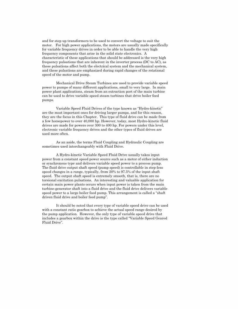
Figure 1. “Hydro-kinetic” Variable Speed Fluid Drive

Figure 2. Sizing Chart for Fluid Drives Hydraulic Diameters are Shown on Diagonal.

For Example, “370” Signifies 37.0 Inches.

Design of Hydro-kinetic Variable Speed Fluid Drives: The design of a “Hydro-kinetic” Variable Speed Fluid Drive with an oil conditioning system is shown in Figure 1. The primary mechanical components of a variable speed fluid drive assembly are (a) an outer housing or tank that supports the bearings, holds the oil, and provides a protective cover, (b) an input element comprising an input shaft and coupling hub, an impeller, an intermediate casing, and an outer casing (or scoop tube casing) all attached to each other and rotating together, (c) an output element comprising an output shaft, a coupling hub, and a runner all attached to each other and rotating together, (d) journal and thrust bearings that support each shaft, (e) oil used as a power transmitting medium between the impeller and runner and as a lubricant for the bearings, (f) a moveable scoop tube that slides in and out to control the amount of oil that remains resident in the rotating casings; and (g) an oil conditioning system. The impeller and runner are structures with vanes and pockets between the vanes shaped much like a half of a grapefruit with the linings that separate the fruit intact and the fruit removed. The impeller and a runner face each other with a small gap between them, on the order of 1% of the diameter of the impeller (or runner), but they do not touch each other mechanically. The impeller and the attached rotating casing structure retain the working fluid, usually oil, as shown in Figure 1. The runner is located within the envelope of the rotating input element. The actual mechanism causing the runner to rotate is the kinetic action of the oil: the impeller transmits energy to the oil and the oil transmits energy to the runner, as described below. Fluid Drives of the Variable Speed Fluid Drive type are sized according to the equation: Power (hp) = Factor x Nout^3 x Dia^5 10^14 Where: Factor = approximately 2.1, but depends on many design details such as exact pocket shape, vane angles, and the circuit oil flow rate. N out = 0.975 x N in (rated speed point) (rpm) Dia = Hydraulic diameter of the impeller and runner (inches). Figure 2 is a chart showing power (hp and kw) as a function of speed for various hydraulic diameters. The actual sectors that are applicable for different hydraulic diameters will vary slightly depending upon the many design details of a drive. Consequently, this chart should be considered to

represent trends for different fluid drives, but should not be considered to represent a specific fluid drive. A fluid drive of the Hydro-kinetic Variable Speed design operates as follows: The tank contains a level of oil, often described as ISO VG 32, as light turbine oil. An oil pump supplies cooled and filtered “lube oil” to the bearings and “circuit oil” or “working oil” to the “circuit” meaning the cavity comprising the pockets between the vanes of the impeller and runner, as shown in Figure 1. Because the impeller and runner are rotating, the circuit oil is thrown outward under centrifugal force, so that the oil forms a torus in the rotating casing assembly. Because the impeller is being driven by a driver, generally at a fixed speed, the impeller rotates faster than the runner. Consequently, oil that is in the impeller is subject to greater centrifugal acceleration than is oil that is located in the runner pockets. Consequently, a parcel of oil that starts in an impeller pocket moves in a generally circular path (relative to the rotating pocket) to the radially outer portion of that impeller pocket, gaining momentum along the path, and leaves the impeller pocket traveling across the gap with both circumferential and axial velocity components, then the packet of oil enters a runner pocket where because the runner is rotating slower than the impeller, the oil packet hits the wall of that runner pocket, and departs momentum to the runner vane, after which the packet of oil moves radially inward along a generally circular path (relative to the runner pocket) until it leaves the runner pocket in a path with axial and circumferential velocity components, until the packet of oil enters an impeller pocket where because the impeller is rotating faster than the runner, the wall of that impeller pocket hits the packet of oil and imparts momentum to the packet of oil, and then the packet of oil again follows a circular path (relative to the impeller pocket) radially outward within the impeller pocket until it again crosses the gap to enter the runner. The combination of both circular paths within the pockets and a circumferential path of the pockets around the shaft centerline provides a general trajectory of each packet of oil that is a spiral that travels in circles, as shown in Figure 3.

Note that in a Hydro-kinetic Fluid Drive, the energy is transmitted from impeller to runner using the principal of “momentum exchange”: The vane of the impeller hits a packet (mass) of oil and increases its velocity, and then the packet (mass) of oil hits the vane of a runner and the velocity of the oil is reduced, transmitting momentum, and the process continues. Fluid drives are “constant torque” machines, that is, the torque that is absorbed by the impeller from the input shaft to drive the circuit oil equals the torque that the circuit oil imparts to the runner that drives the output shaft and the load, which, in the present case, is a pump.

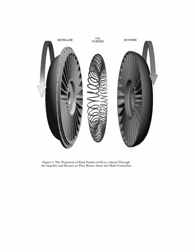
Figure 3. The Trajectory of Each Packet of Oil is a Spiral Through

the Impeller and Runner as They Rotate about the Shaft Centerline.

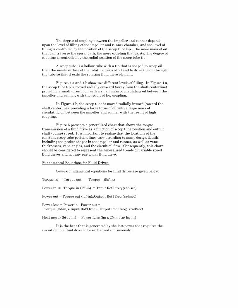
The degree of coupling between the impeller and runner depends upon the level of filling of the impeller and runner chamber, and the level of filling is controlled by the position of the scoop tube tip. The more mass of oil that can traverse the spiral path, the more coupling that exists. The degree of coupling is controlled by the radial position of the scoop tube tip. A scoop tube is a hollow tube with a tip that is shaped to scoop oil from the inside surface of the rotating torus of oil and to drive the oil through the tube so that it exits the rotating fluid drive element.

Figures 4.a and 4.b show two different levels of filling. In Figure 4.a, the scoop tube tip is moved radially outward (away from the shaft centerline) providing a small torus of oil with a small mass of circulating oil between the impeller and runner, with the result of low coupling. In Figure 4.b, the scoop tube is moved radially inward (toward the shaft centerline), providing a large torus of oil with a large mass of circulating oil between the impeller and runner with the result of high coupling. Figure 5 presents a generalized chart that shows the torque transmission of a fluid drive as a function of scoop tube position and output shaft (pump) speed. It is important to realize that the locations of the constant scoop tube position lines vary according to many design details including the pocket shapes in the impeller and runner, as well as vane thicknesses, vane angles, and the circuit oil flow. Consequently, this chart should be considered to represent the generalized trends of variable speed fluid drives and not any particular fluid drive. Fundamental Equations for Fluid Drives: Several fundamental equations for fluid drives are given below: Torque in = Torque out = Torque (lbf-in) Power in = Torque in (lbf-in) x Input Rot’l freq (rad/sec) Power out = Torque out (lbf-in)xOutput Rot’l freq (rad/sec) Power loss = Power in - Power out = Torque (lbf-in)x(Input Rot’l freq - Output Rot’l freq) (rad/sec) Heat power (btu / hr) = Power Loss (hp x 2544 btu/ hp-hr) It is the heat that is generated by the lost power that requires the circuit oil in a fluid drive to be exchanged continuously.

Figure 4.a. A Small Torus of Circuit Oil Provides Small Coupling.

Figure 4.b. A Large Torus of Circuit Oil Provides Large Coupling.

Certain losses are not included in the above equations. These include bearing power losses and circuit oil handling losses. Bearing losses for the input shaft are constant and for the output shaft increase with increasing speed. Circuit oil handling losses are a function of scoop tube position and circuit oil flow rate. Most fluid drives have a constant, or almost constant, circuit oil flow rate, so the circuit oil handling losses are greatest when the scoop tube tip is at the largest distance from the shaft centerline, which corresponds to minimum output shaft (or pump) speed, and these losses are the least when the scoop tube tip is closest to the shaft centerline, which corresponds to maximum output shaft (or pump) speed. The net result is that the sum of the bearing losses and circuit oil handling losses can be considered to be a constant, typically ranging from 3 % to 4 % of the rated power of the fluid drive. The efficiency of a variable speed fluid drive of the hydro-kinetic type can typically be expressed as Efficiency = Output shaft speed - 3.5 % Input shaft speed It is very common to use a slip speed (Input speed - Output speed) of 2.5% at the design point, though in some applications, the slip speed at the rated operating point is between 2.0 % to over 4 % . Using a slip speed of 2.5% at the design point, the design point efficiency is 100% - 2.5% (slip speed loss) - 3.5% (mechanical losses) = 94% . If a set of gears is included within the fluid drive tank and it is located on the output side of the fluid drive circuit, the runner output shaft and a gear shaft can be combined, eliminating two journal bearings and a pair of thrust bearings. In this case, the power losses will increase by approximately 1.5 %, rather than the normal 2.0 to 2.5 % additional loss when an independent gear box is used between the fluid drive and the pump. Comparison of Efficiencies of Variable Speed Drives: When comparing efficiencies for alternative types of variable speed drives, it is essential to determine the following factors: First, before the efficiency is calculated it is essential to determine if the equipment being evaluated will provide variable speed power under all of the conditions that are required ? Second, determine if the equipment will respond as fast to a change of load as is required or desired ? Third, determine if the efficiency of alternate types of equipment will be evaluated at several operating points from low load, say 20%, to full load being included, or will the evaluation be based on only one operating point, such as full power ? Many types of equipment can be designed to operate well at or near a single operating point such as full load, but they do not perform well when operating away from the design point of full load.

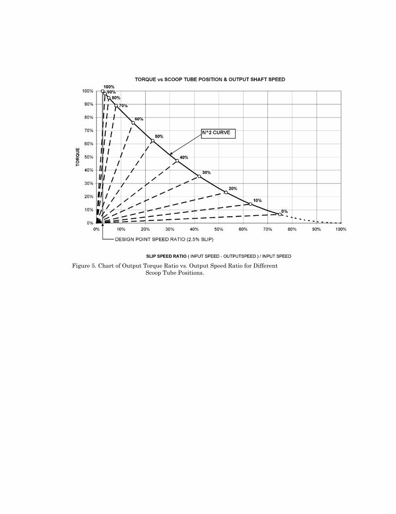
Figure 5. Chart of Output Torque Ratio vs. Output Speed Ratio for Different

Scoop Tube Positions.

A good way to evaluate alternative forms of variable speed drives is to examine the annual costs for operating each complete drive train at several operating points, giving weight for each load point in proportion to the number of hours that the equipment is expected to operate at each of these points during a year. The reason is that when operating at or near full load, there is high power, there is high efficiency, and there are usually a large number of hours, so the actual costs at this operating point are quite favorable. Then there are times when the drive train and pump will be operating at low load, at which time the efficiency is low, very little power is transmitted, and the number of hours at this point is limited, with the consequence that, when averaged with the high efficiency operating points at high load conditions, the average efficiency is quite satisfactory. When performing these evaluations, it is very critical that an accurate value of the actual power consumption for each evaluation point be obtained and used. This includes such things as (a) for steam turbines, the actual heat rate at “off design” conditions when extraction steam is not available in sufficient quantity and main steam or steam from a “pony boiler” may be needed, and (b) for electronic variable frequency drives, the air conditioning load for the electronics as well as the transformer, wiring, and motor losses, especially the losses due to the very high frequencies. . Construction of Fluid Drives and the Oil Conditioning Systems: Variable speed fluid drives are built by a number of manufacturers around the world. Most manufacturers have developed a range of designs of fluid drives for specific applications, and these that have become “standardized lines” for that manufacturer. Many applications require specialized designs that are not among the standardized designs, due to the environment, power, speed, or turn down conditions, and upon request, manufacturers will often provide those specialized designs. Fluid drives can be made with horizontal shafting or vertical shafting. The materials of construction of fluid drives vary widely. Outer housings and certain bearing housings are usually made of fabricated steel, may be split horizontally or may be stacked from one end, and may be made from thick steel or from thin steel. In certain cases, the outer housings and certain bearing housings may be made of cast iron or cast steel. The impellers and runners may be cast aluminum of a variety of grades and heat treats, cast steel, fabricated steel, or milled from solid forgings of alloy steel. For a fluid drive with a hydraulic diameter of 25 to 27 inches, the impeller and runner pockets are each about 6 inches deep axially and the gap between the impeller and runner faces is on the order of 1/4 inch to 3/8 inch. Pocket sizes and gaps for other fluid drive sizes are larger or smaller in proportion to the size of the fluid drive hydraulic diameter. Shafts and other rotating casings are usually made of carbon steel or alloy steel. Heat treatment may or may not be used. The journal and thrust bearings can be rolling element design or Babbitted bearings, and the choice

depends upon the speed, size limitations, operating duty, required life, and price. Rolling element bearings come in a range of duties and L10 (or B10) lives. Babbitted bearings may be made of simple fixed shapes or they can be made with extremely robust tilting pad designs. Flexible coupling types range from gear to diaphragm styles, and they may be supplied by the customer, by the manufacturer, or in some cases, the hubs may be made integral with the shafts. Instrumentation such as thermocouples or resistance temperature devices (RTDs) and vibration pickups, proximity or seismic, may or may not be included. Oil conditioning systems can be extremely simple, comprising one pump, electric or shaft driven, one cooler, one filter, and one sight glass to determine the oil level in the tank. Alternately, they can be quite complex being built according to the highest level of API specifications with duplex AC main oil pumps, a DC emergency pump, duplex oil coolers, duplex filters, all stainless steel piping, various isolation valves, pressure control valves, actuator for the scoop tube, additional lube oil requirements for the main motor and main pump, and with electronic transmitters for pressure, temperature, and oil levels for interfacing with DCS systems. Because there are no industry standards that broadly apply to all fluid drives, it is essential for the user to detail all of the desired features in the purchasing specification. As will be seen below, the heat loss in a fluid drive depends upon the specific operating points in the application, and several operating points should be provided to the manufacturer, including the maximum power and speed point, the minimum power and speed point, and two or three interim operating points, especially the lowest pressure with the maximum flow. The reason for providing such details is that there is no reason to use larger pumps and/or larger heat exchangers than are required to meet the user’s operating conditions and, at the same time, to maintain the maximum oil temperatures below the oxidation limits of the particular oil to be used (generally in the range of 185 degrees F). When gears are included in the mechanical design of the fluid drive, the service factors for gear sets located on the output side of the fluid drive do not need to be so high as when they are located on the input side, particularly when synchronous motors are involved. Because there is such a wide range of design features that can be used in fluid drives, and because the technology content is the principal controller of price, the pricing can vary widely for different fluid drives for the same maximum power and maximum speed. In other words, specifications addressing only the max speed and max power are not sufficient to specify a fluid drive adequately, especially the oil system for a fluid drive, because the most difficult operating points for fluid drives are in the “turn down” operating points when the output shaft speed is in the neighborhood of 2/3 of the input shaft speed. It is extremely helpful to the fluid drive manufacturer/designer if the user actively participates in developing the design details of the equipment. When a Variable Speed Fluid Drive and its mating Oil Conditioning System are properly designed for a given application, they become relatively simple mechanical systems with extremely high reliability and availability. It is quite common for variable speed fluid drives to operate for over ten years without inspection or any maintenance other than changing oil filters. When

maintenance of a fluid drive is required, parts can be obtained or can be made as required. It is rare for a fluid drive design to become obsolete, which has been a problem on certain types of electronic variable frequency drives. The speed of the output rotating assembly is controlled by the position of the scoop tube tip which is typically positioned by a scoop tube actuator, being driven by a 4-20 ma signal from the plant control system, such as the central DCS (Distributed Control System), for the entire process unit. It is interesting to note that the Fluid Drive of the Hydro-kinetic design was invented by Dr. Herman Fottinger in Germany in 1905, and fluid drives of this design are now used all over the world. A textbook on Fluid Drives, also called Fluid Couplings, that may be useful to those who have an interest in technical details is entitled Stromungskupplungen und Stromungswandler, Berechnung und Konstruction, by Ing. Maurizio Wolf, Springer-Verlag, Berlin/Gottingen / Heidelberg, 1962. Fluid Drive designs have been tuned and adjusted and adapted to many applications, but the fundamental features, other than instrumentation, have not significantly changed. Power Loss and Temperature Conditions for Variable Speed Fluid Drives. A very simplified approach for evaluating the heat loss of a variable speed drive assumes that the power required by a pump is only proportional to the cube of the pump speed (or output shaft speed). This is correct under certain conditions, but because pumps operate at points on the head-capacity plot that are at some distance from this simplified curve, a more appropriate evaluation of the heat loss of a variable speed fluid drive for boiler feed pump service is given below via a series of head-capacity Charts. In the simplified approach, assume that the power of a pump is proportional to the cube of the pump speed (or fluid drive output shaft speed ): Power out = N out ^ 3 And Torque out = N out^2. Now Torque in = Torque out = Torque, Hence Power in = Torque in x N in Power in = N out^2 x N in Power Loss = Power in - Power out = N out^2 x N in - N out ^ 3 The maximum loss occurs at N out = 2 x Nin 3

The maximum loss at this output shaft (pump) speed is approximately 15% of the rated input power. Including bearing and circuit oil handling losses, the maximum loss is on the order of 16% to 17 % of the rated input power. The circuit oil flow pattern within the fluid drive chamber consisting of the impeller pockets and runner pockets and the axial gap between them can be considered to be a spiral in general, Figure 3, but it is extremely turbulent. The turbulence of the circuit oil is affected by the speed difference, the torque transmitted, and the amount of circuit oil in the rotating element. As indicated above, the speed at which the maximum power loss occurs is when the output shaft is at approximately 2/3 of the input shaft speed, which is also the speed at which the greatest turbulence occurs. Thus, for a fluid drive input speed of 3600 rpm, the maximum turbulence occurs when the output shaft speed (pump speed) is in the range of 2400 rpm. It is also important to note that for a given output shaft speed both the turbulence and the power loss increases with increased torque. Five head-capacity charts are provided below that are based on the head-capacity plot for a main boiler feed pump for a 375 MW Turbine-Generator. The head is shown in units of psig because the intent of these charts is to show trends for understanding of the issues at hand rather than to be completely accurate. For specific applications, the grids can be calculated with all of the normal details considered, but it will not change the principles at hand. The grids on the charts are made of constant speed lines (generally horizontal) and constant efficiency lines (generally curving upward). The grids are for the same conditions on all of the charts. Data is presented at certain intersection points of the grids. Figure 6 (Chart 1) presents the shaft power absorbed by the pump (out of the fluid drive). Figure 7 (Chart 2) presents the shaft power absorbed by the fluid drive (out of the motor or Turbine-Generator) at the same intersection points of the same grid. Figure 8 (Chart 3) presents the power lost to the circuit oil in the element (power into the fluid drive minus power out of the fluid drive). Figure 9 (Chart 4) presents the Circuit Oil Discharge temperature that results from the power lost in Chart 3 with the circuit oil input temperature of 120 deg F and a constant circuit oil flow rate of 400 gpm. Figure 10 (Chart 5) presents the circuit oil flow rate (gpm) required to maintain a constant temperature rise of the circuit oil (the difference between the circuit oil temperature entering the fluid drive and the circuit oil discharge (COD) temperature from the fluid drive rotating element. For instance, in Figures 6 through 10 ( Charts 1 through 5), following the constant speed line for 2400 rpm from left to right, it can be

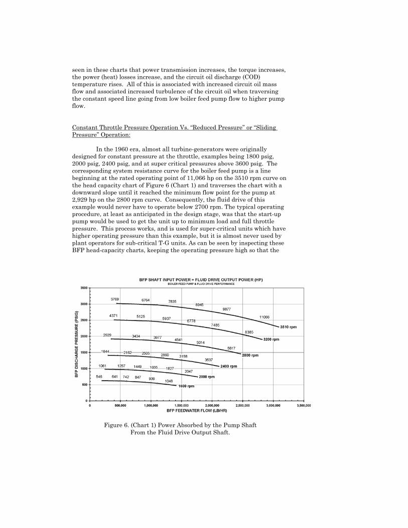
seen in these charts that power transmission increases, the torque increases, the power (heat) losses increase, and the circuit oil discharge (COD) temperature rises. All of this is associated with increased circuit oil mass flow and associated increased turbulence of the circuit oil when traversing the constant speed line going from low boiler feed pump flow to higher pump flow.

Constant Throttle Pressure Operation Vs. “Reduced Pressure” or “Sliding Pressure” Operation: In the 1960 era, almost all turbine-generators were originally designed for constant pressure at the throttle, examples being 1800 psig, 2000 psig, 2400 psig, and at super critical pressures above 3600 psig. The corresponding system resistance curve for the boiler feed pump is a line beginning at the rated operating point of 11,066 hp on the 3510 rpm curve on the head capacity chart of Figure 6 (Chart 1) and traverses the chart with a downward slope until it reached the minimum flow point for the pump at 2,929 hp on the 2800 rpm curve. Consequently, the fluid drive of this example would never have to operate below 2700 rpm. The typical operating procedure, at least as anticipated in the design stage, was that the start-up pump would be used to get the unit up to minimum load and full throttle pressure. This process works, and is used for super-critical units which have higher operating pressure than this example, but it is almost never used by plant operators for sub-critical T-G units. As can be seen by inspecting these BFP head-capacity charts, keeping the operating pressure high so that the

Figure 6. (Chart 1) Power Absorbed by the Pump Shaft From the Fluid Drive Output Shaft.

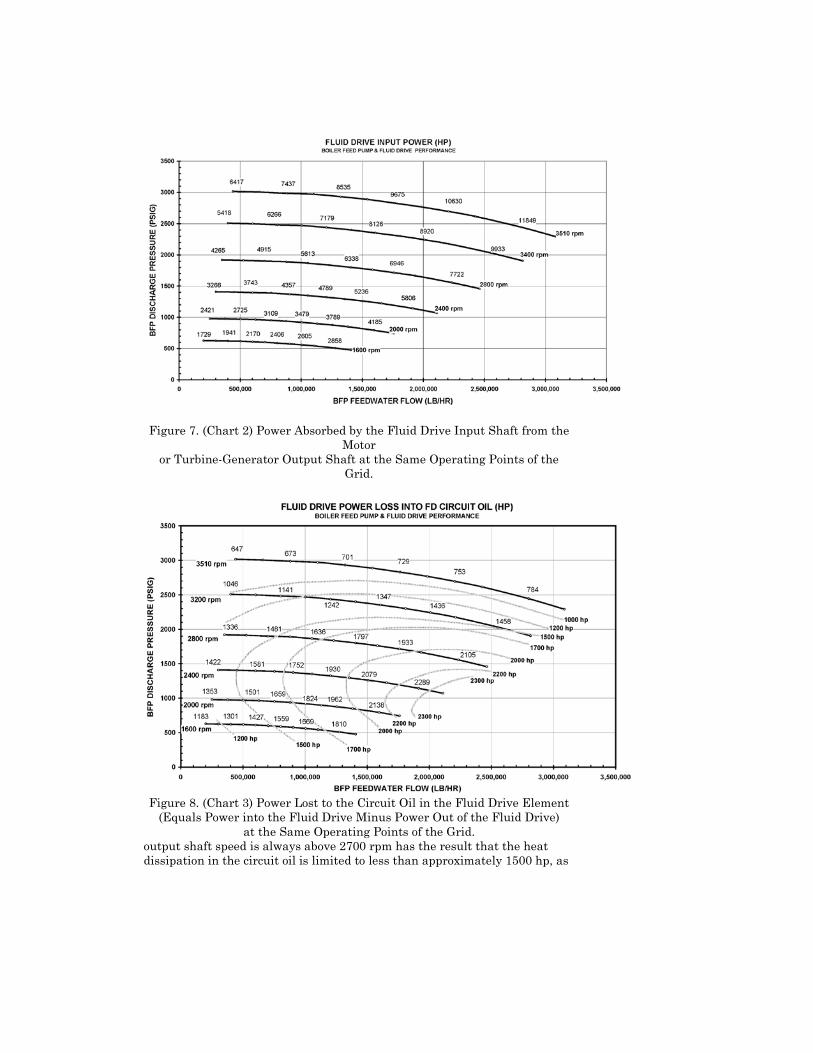
Figure 7. (Chart 2) Power Absorbed by the Fluid Drive Input Shaft from the Motor

or Turbine-Generator Output Shaft at the Same Operating Points of the Grid.

Figure 8. (Chart 3) Power Lost to the Circuit Oil in the Fluid Drive Element

(Equals Power into the Fluid Drive Minus Power Out of the Fluid Drive) at the Same Operating Points of the Grid.

output shaft speed is always above 2700 rpm has the result that the heat dissipation in the circuit oil is limited to less than approximately 1500 hp, as

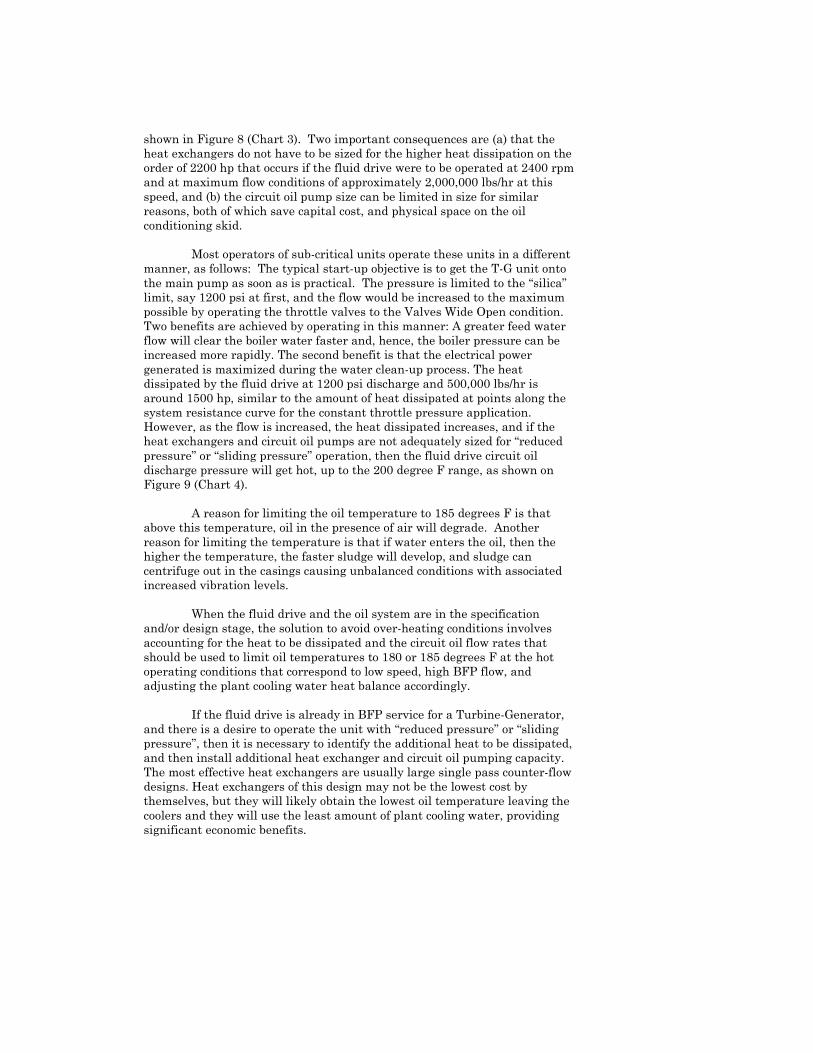
shown in Figure 8 (Chart 3). Two important consequences are (a) that the heat exchangers do not have to be sized for the higher heat dissipation on the order of 2200 hp that occurs if the fluid drive were to be operated at 2400 rpm and at maximum flow conditions of approximately 2,000,000 lbs/hr at this speed, and (b) the circuit oil pump size can be limited in size for similar reasons, both of which save capital cost, and physical space on the oil conditioning skid. Most operators of sub-critical units operate these units in a different manner, as follows: The typical start-up objective is to get the T-G unit onto the main pump as soon as is practical. The pressure is limited to the “silica” limit, say 1200 psi at first, and the flow would be increased to the maximum possible by operating the throttle valves to the Valves Wide Open condition. Two benefits are achieved by operating in this manner: A greater feed water flow will clear the boiler water faster and, hence, the boiler pressure can be increased more rapidly. The second benefit is that the electrical power generated is maximized during the water clean-up process. The heat dissipated by the fluid drive at 1200 psi discharge and 500,000 lbs/hr is around 1500 hp, similar to the amount of heat dissipated at points along the system resistance curve for the constant throttle pressure application. However, as the flow is increased, the heat dissipated increases, and if the heat exchangers and circuit oil pumps are not adequately sized for “reduced pressure” or “sliding pressure” operation, then the fluid drive circuit oil discharge pressure will get hot, up to the 200 degree F range, as shown on Figure 9 (Chart 4). A reason for limiting the oil temperature to 185 degrees F is that above this temperature, oil in the presence of air will degrade. Another reason for limiting the temperature is that if water enters the oil, then the higher the temperature, the faster sludge will develop, and sludge can centrifuge out in the casings causing unbalanced conditions with associated increased vibration levels. When the fluid drive and the oil system are in the specification and/or design stage, the solution to avoid over-heating conditions involves accounting for the heat to be dissipated and the circuit oil flow rates that should be used to limit oil temperatures to 180 or 185 degrees F at the hot operating conditions that correspond to low speed, high BFP flow, and adjusting the plant cooling water heat balance accordingly. If the fluid drive is already in BFP service for a Turbine-Generator, and there is a desire to operate the unit with “reduced pressure” or “sliding pressure”, then it is necessary to identify the additional heat to be dissipated, and then install additional heat exchanger and circuit oil pumping capacity. The most effective heat exchangers are usually large single pass counter-flow designs. Heat exchangers of this design may not be the lowest cost by themselves, but they will likely obtain the lowest oil temperature leaving the coolers and they will use the least amount of plant cooling water, providing significant economic benefits.

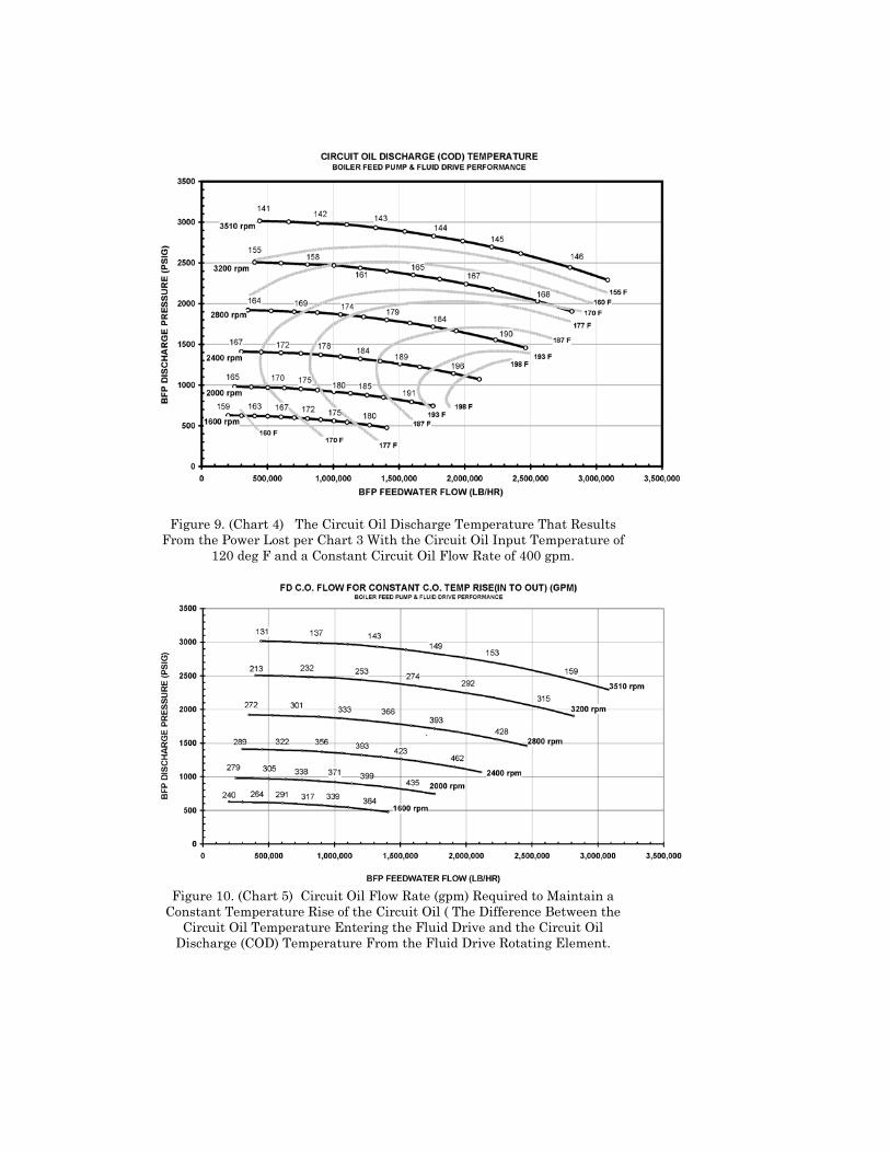
Figure 9. (Chart 4) The Circuit Oil Discharge Temperature That Results From the Power Lost per Chart 3 With the Circuit Oil Input Temperature of

120 deg F and a Constant Circuit Oil Flow Rate of 400 gpm.

Figure 10. (Chart 5) Circuit Oil Flow Rate (gpm) Required to Maintain a

Constant Temperature Rise of the Circuit Oil ( The Difference Between the Circuit Oil Temperature Entering the Fluid Drive and the Circuit Oil

Discharge (COD) Temperature From the Fluid Drive Rotating Element.

While more heat is lost in a fluid drive on sliding pressure operation than on constant throttle pressure, the amount of power saved in the pumping process and in the reduction of throttling losses in the steam turbine is greater, providing a substantial net improvement in the overall cycle efficiency. For instance, the input power to the fluid drive in Figure 6 at full pressure and 350,000 lbs/hr is 4265 hp, whereas on sliding pressure conditions for the same MW, which uses about the same feed water flow, the input power is about 2500 hp, a savings of 1765 hp, or 1.3 MW, which at $70/ MW represents around $100./hour. This savings is only the reduced power to drive the pump, and does not include reduced throttling losses, and reduced fan airflow and other savings. Sliding pressure operation, including unconditional operation anywhere on the head-capacity map, usually has tremendous economic benefits. In most cases where the process can use these capabilities, the improved operating conditions can pay for the slight increase in capital cost for a heavy duty fluid drive and oil system in a matter of a few months. A reference book for analyzing sliding pressure operation in steam turbines is entitled Evaluating and Improving Steam Turbine Performance, by Ken C. Cotton, Second Edition, published by Cotton Fact in 1998. Use of a Control Valve to Maintain Uniform Circuit Oil Discharge (COD) Temperatures: At very low speed - low BFP flow operation, the minimum speed at low or zero % scoop tube is substantially controlled by the circuit oil flow rate. Control of the pump speed, and hence, the BFP flow is improved by minimizing the circuit oil flow to that required to keep the circuit oil discharge (COD) temperature below approximately 185 degrees F. This suggests that circuit oil flows should be reduced, which is the opposite of the solution for the high heat condition discussed above. The compromising solution to this circuit oil flow issue is to install a circuit oil discharge (COD) temperature control valve that limits the circuit oil flow to the fluid drive in order to maintain a constant circuit oil discharge (COD) temperature. Depending upon the application, this COD temperature set point is set in the neighborhood of 180 degrees F. The results of the use of this COD valve are demonstrated in Chart 5, which is based on the heat dissipated in Chart 3 and upon a constant differential temperature (circuit oil discharge temperature - circuit oil supply temperature) of 70 deg F. In this chart, the COD temperature remains constant and the flow varies, whereas in Chart 4, the circuit oil flow is constant and the COD temperature varies. Additional benefits arise: (1) The circuit oil flow is limited in the low output shaft speed range, and this increases the effectiveness of the scoop tube to control the output shaft/pump speed, reducing the minimum output shaft/pump speed when the scoop tube is at the minimum power position, and yielding greatly improved feed water control throughout the low speed range.

(2) The circuit oil pump size can be increased to suit the specific application so that when the fluid drive is operated in the neighborhood of 2400 rpm and it is generating a large amount of heat, the circuit oil flow is adequate to limit the maximum temperature of the circuit oil discharging from the fluid drive element to approximately 180 to 185 deg F. (3) The power required to handle the circuit oil is reduced at operating conditions away from the high heat zone, increasing the operating efficiency of the unit. (4) A constant temperature fluid drive maintains uniform elevation height of the input and output shafts and maintains uniform thermal expansion of the housing and all internal parts. This extends the life of the fluid drive by minimizes low cycle stresses, relative movement, or fatigue of the various parts. It should be noted that TRI has been awarded US Patent 5,315,825 regarding the use of a circuit oil flow control valve that is controlled via a feedback from the COD Temperature Instrument, as described above.

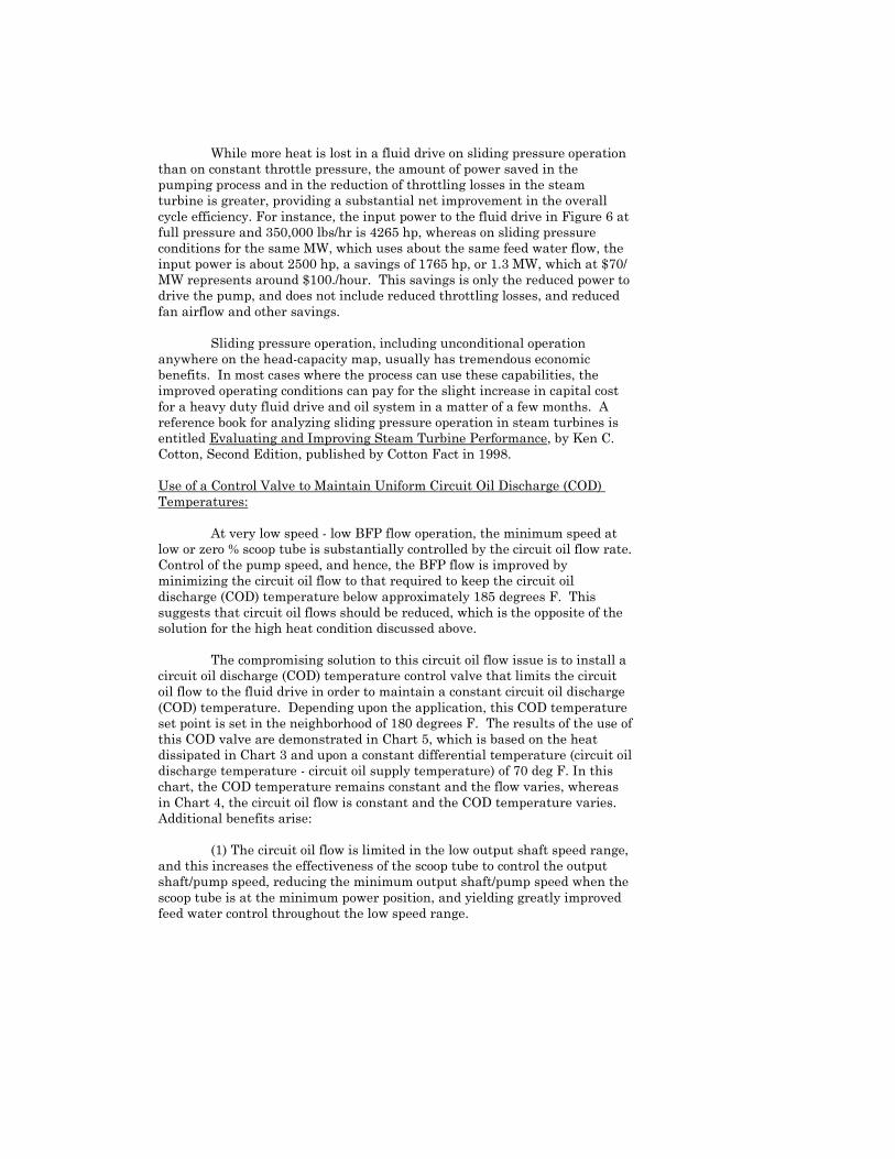
Typical Vibrations of High Power Variable Speed Fluid Drive Rotors: In almost every fluid drive, the first critical speed of the input shaft and the first critical speed of the output shaft is each measurably above 3600 rpm (60 hz). The mode of vibration of each shaft in response to unbalance is typically a rigid body conical mode. That is, there is almost no bending of the shaft and the critical speed of each shaft is controlled primarily by the stiffnesses of the oil films of the bearings and the structures that support the bearings for that shaft. Depending upon the condition of the journal bearings, it is possible to experience some sub-synchronous vibration such as “oil whip” which occurs at a fractional frequency, generally below half running speed. This type of vibration should not be confused with a very unique type of vibration that often arises in fluid drives, discussed below: The journal at the input-inboard bearing of a high powered variable speed fluid drive typically has the highest amplitude vibrations because it is this journal that is experiencing the largest vibratory forces, both from the heavy casings of the input rotor and from the unbalance of the turbulent oil contained in these casings. A typical vibration frequency analysis for this input-inboard journal appears is shown in Figure 11. The unique features of this figure are that three vibration components usually appear in this analysis: (a) the synchronous component of the input shaft, which in this case is 60 hz, (b) the output shaft rotational frequency, 39 hz, and (c) a frequency (41 to 44 hz) that is slightly above the output shaft rotational frequency corresponding to the average effective rotational frequency of the circuit oil in the rotating element.

Figure 11. A Typical Vibration Frequency Analysis of the Journal at the Input-Inboard Bearing of a High Power Variable Frequency Fluid Drive

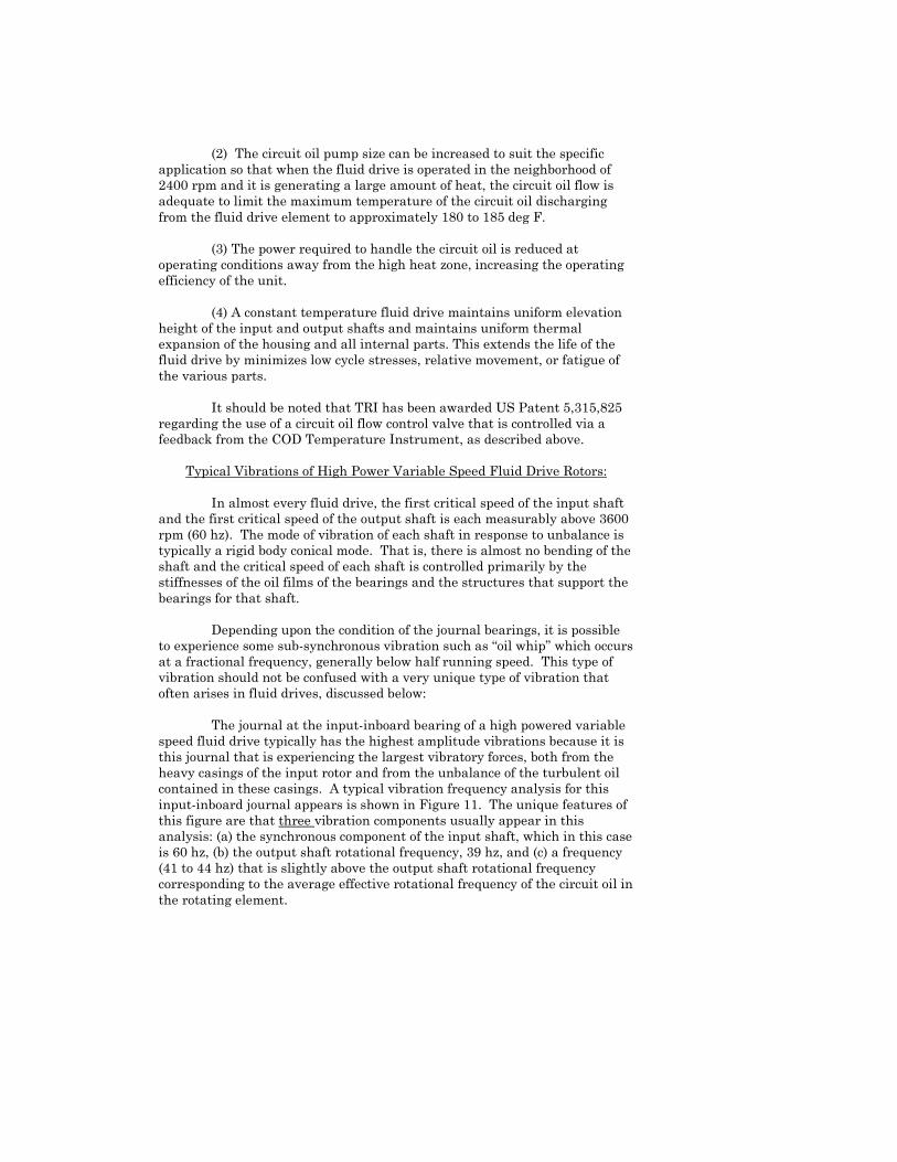
Figure 12. Variable Speed Geared Fluid Drive with Parallel Start-up

Capability that is Used to Start a Very Large Motor Which can Then Drive a Very Large Pump, Courtesy, Turbo Research, Inc..

Alternate Arrangements of Drivers, Fluid Drives, and Boiler Feed Pumps for Turbine-Generator Service: These days, there is great emphasis of improving the overall efficiency of fossil-fired generating plants. It is very common to design every new plant as if it is going to operate at only one point: full load. However, once built, many have to cycle to a reduced load at night, and this includes those that use fossil fuels. In this case, having the unit designed so that it is relatively efficient at full load as well as over a range of operating points down to low load is more appropriate. To this end, an arrangement that should be considered is one wherein the fluid drive and 100 % capacity boiler feed pump are attached directly to a steam turbine-generator extension shaft, and to have the entire plant designed for sliding pressure at the turbine throttle valve. In the 1960s, many such steam turbine-generators were built this way, that is, with a single 100 % “shaft driven” fluid drive/ boiler feed pump attached to either the turbine or generator extension shaft. A number of these units had heat rates at the design point on the order of 9300 btu /kw-hr. Several were built at the 325 MW range. Ravenswood 3, then owned by Consolidated Edison of New York, Inc., was the first 1000 MW unit in the world and was commissioned in 1965. It was built for sliding pressure and, incidentally, it had coal fired boilers. This is a cross-compound unit, and there are two fluid drive/boiler feed pumps, each rated at 18,000 hp, one set on each end of the HP / IP Turbine / Generator 3600 rpm shaft line. With today’s technology, a single fluid drive / boiler feed pump set on the order of 36,000 hp could be used instead of the two that were used then. Consequently, today, with the availability of three-dimensional computational flow dynamic analyses for steam path design, it should be possible to build large electrical generating plants using similar arrangements and obtain net heat rates measurably below 9000 btu / kw-hr. The primary advantage of the “shaft driven” design is purely to maximize efficiency of the steam power. In the shaft driven arrangement, the steam power is converted to mechanical power at approximately 92 % efficiency. Near the maximum power point, the efficiency of a fluid drive is around 93 % at full load, and it will exceed 70% for the bulk of the hp-hours of operation, though it will drop below that for very low load operation. In comparison, very few mechanical drive steam turbines exceed 70 % efficiency at the best operating points. For a motor driven fluid drive and pump arrangement, the power supply chain is longer and less efficient: The mechanical power at the turbine coupling to the generator is 92 % of the steam power (the same as

above), with additional losses of approximately 1.6% for the generator, 1% for the transformer, and perhaps 6% for the motor. The result is that for every MW needed to drive a fluid drive by a motor requires at least 9% more of the power from the turbine shaft. For a 1000 MW T-G that requires 36,000 hp from the turbine to drive a boiler feed pump via the “shaft driven” feature would require 39,234 hp, or an additional 3,234 hp to drive a motor driven boiler feed pump. This is significant in heat rate calculations for a Turbine-Generator of this size. Variable Speed Fluid Drive for Large Synchronous Motors with a Starting Capability: As mentioned above, with today’s technologies, it is possible to build very large 100% boiler feed pumps and comparably large fluid drives for Turbine-Generators on the order of 900 to 1300 MW. Figure 12 presents an example of a fluid drive design that can be used for the unique application of a very large synchronous motor driving a geared fluid drive / large boiler feed pump. This variable speed geared fluid drive has features (a) to start a very large synchronous motor so that this very large motor can be connected to the grid smoothly without a large inrush current, (b) to separate the starting equipment from the gear train, and then (c) to use the large motor to drive a comparably large variable speed pump. This design permits the use of one large motor / fluid drive / boiler feed pump to be used from start-up to full load operation. No start-up boiler is required as is required if a steam turbine driver is used, and no small start-up boiler feed pump is required as is required for a shaft driven fluid drive / boiler feed pump. The consequence is that a wide range of options for driving large boiler feed pumps, and other pumps as well, is now available to system designers. Beyond those fluid drive arrangements discussed here are alternative configurations that can be adapted or developed to meet the needs of these and other applications.