VARIABLE-SPEED, ROBUST SYN-

CHRONOUS RELUCTANCE MACHINE

DRIVE SYSTEMS

Project title: Variabel hastighed, robust synkron reluctance motor drev systemer

Project data: Journalnr.: 464-11,

project nr.: 344-068

Auditor: Assoc. Professor Kaiyuan Lu; Ph. D. student Dong Wang

Address: Aalborg University, Department of Energy Technology, Pontoppidanstraede 101,

room 39, DK-9220 Aalborg East

- 1 -

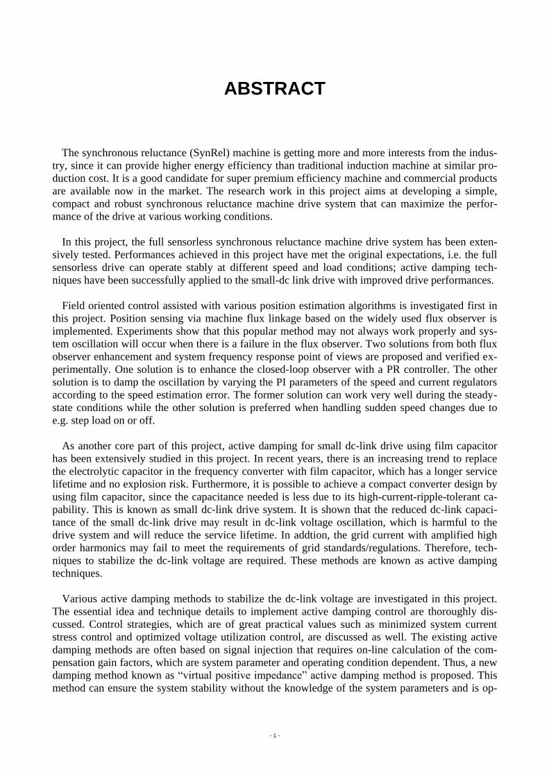
ABSTRACT

The synchronous reluctance (SynRel) machine is getting more and more interests from the indus-

try, since it can provide higher energy efficiency than traditional induction machine at similar pro-

duction cost. It is a good candidate for super premium efficiency machine and commercial products

are available now in the market. The research work in this project aims at developing a simple,

compact and robust synchronous reluctance machine drive system that can maximize the perfor-

mance of the drive at various working conditions.

In this project, the full sensorless synchronous reluctance machine drive system has been exten-

sively tested. Performances achieved in this project have met the original expectations, i.e. the full

sensorless drive can operate stably at different speed and load conditions; active damping tech-

niques have been successfully applied to the small-dc link drive with improved drive performances.

Field oriented control assisted with various position estimation algorithms is investigated first in

this project. Position sensing via machine flux linkage based on the widely used flux observer is

implemented. Experiments show that this popular method may not always work properly and sys-

tem oscillation will occur when there is a failure in the flux observer. Two solutions from both flux

observer enhancement and system frequency response point of views are proposed and verified ex-

perimentally. One solution is to enhance the closed-loop observer with a PR controller. The other

solution is to damp the oscillation by varying the PI parameters of the speed and current regulators

according to the speed estimation error. The former solution can work very well during the steady-

state conditions while the other solution is preferred when handling sudden speed changes due to

e.g. step load on or off.

As another core part of this project, active damping for small dc-link drive using film capacitor

has been extensively studied in this project. In recent years, there is an increasing trend to replace

the electrolytic capacitor in the frequency converter with film capacitor, which has a longer service

lifetime and no explosion risk. Furthermore, it is possible to achieve a compact converter design by

using film capacitor, since the capacitance needed is less due to its high-current-ripple-tolerant ca-

pability. This is known as small dc-link drive system. It is shown that the reduced dc-link capaci-

tance of the small dc-link drive may result in dc-link voltage oscillation, which is harmful to the

drive system and will reduce the service lifetime. In addtion, the grid current with amplified high

order harmonics may fail to meet the requirements of grid standards/regulations. Therefore, tech-

niques to stabilize the dc-link voltage are required. These methods are known as active damping

techniques.

Various active damping methods to stabilize the dc-link voltage are investigated in this project.

The essential idea and technique details to implement active damping control are thoroughly dis-

cussed. Control strategies, which are of great practical values such as minimized system current

stress control and optimized voltage utilization control, are discussed as well. The existing active

damping methods are often based on signal injection that requires on-line calculation of the com-

pensation gain factors, which are system parameter and operating condition dependent. Thus, a new

damping method known as “virtual positive impedance” active damping method is proposed. This

method can ensure the system stability without the knowledge of the system parameters and is op-

- 2 -

erating condition independent. A simple compensation gain factor may be introduced when apply-

ing the ‘virtual positive imdedance’ active damping method, which can easily control the level of

the damping effects according to different system performance requrements. This method improves

the existing active damping techniques and is verified experimentally.

Finally, in this project, the preferred flux linkage based position sensorless control with adaptive

PI controllers is used and cooperated with different active damping control methods to drive the

small dc-link SynRel machine drive system. The possible interaction between sensorless control

and active damping control is investigated, and the solution to achieve a simple and robust variable-

speed SynRel machine drive system is proposed. The experimental results show that the introduc-

tion of the small dc-link and active damping control algorithms brings very little impact to the per-

formance of the position-sensorless drive. The influence at steady state conditions is negligible.

Generally, the system can operate satisfactorily and is robust enough to meet different operation

conditions.

In the following sections of this report, first the background and project objectives are given. The

detailed information regarding implementation of the small dc-link SynRel machine drive system is

presented afterwards. Position sensorless control method and achieved results are given next. Anal-

ysis of the small dc-link system is then introduced to cover the important fundamentals in under-

standing small dc-link drive system stability issues. This is followed by the presentation of active

damping methods implemented in this project. Full sensorless operation of this small dc-link Syn-

Rel machine drive system is demonstrated at the end. Finally, conclusion and suggestions for future

work is summerized.

This project is co-financed by Lodam A/S and Dansk Energi (ELFORSK). The whole project was

conducted by a Ph. D. student and was carried out at the Department of Energy Technology, Aalbog

University, Denmark.

- 3 -

1 PROJECT INTRODUCTION

1.1 Background

Energy saving and emission reduction have received tremendous attentions in the past decade.

Use of Variable Speed Drive (VSD) for achieving high system efficiency is an important focusing

area. Previously, Permanent Magnet (PM) machine drive system received the most interest as it fits

this demand satisfactorily. However, the core material of high performance PM machines – rare

earth PM material, experienced a significant increase in price and the price continued to oscillate.

Therefore, high performance permanent-magnet-free electrical drive systems become very interest-

ing and start to receive huge investments in recent years.

The Synchronous Reluctance Machine (SynRM) drive system is believed to be a promising can-

didate. The SynRM has higher torque density and efficiency than that offered by traditional induc-

tion motor (IM) [1], [2], while the cost is in the similar range. The difficulty in obtaining a robust

variable-speed SynRM drive system is on the control side. Its machine parameters, which are used

to derive the necessary information required by the control algorithm, change significantly under

different operating conditions, while IM and PM machine do not suffer a lot from this problem.

Therefore, a simple and robust control method is one of the key issues in implementing a high per-

formance SynRM drive system.

Using small DC-link capacitor is another attracting point in recent drive system developments.

Normally, electrolytic capacitors are used in frequency converters, which may occupy more than

30% of the converter volume. In recent years, there is an increasing trend to replace the electrolytic

capacitor with film capacitor, which has a longer lifetime and no explosion risk. Furthermore, stud-

ies show that the required total capacitance of the dc-link equipped with film capacitors is much

smaller than that equipped with electrolytic capacitors [3], [4]. It is then possible to achieve a com-

pact design by using film capacitors, especially when the voltage and power ratings are high [3], [4].

This is known as small dc-link drive and is obtaining increasing attentions in recent years.

All the above considerations motivate the development of a robust, compact drive system

equipped with SynRM and small dc-link, which has been investigated in this project.

1.2 Project Objectives

In a variable-speed SynRM drive system, rotor motion information, e.g. rotor position and speed,

is essential to ensure the synchronization between the rotor motion and the rotating stator magnetic

field. The motion information may be obtained by auxiliary devices (e.g. resolver, or encoder), but

due to some well-known reasons [5] (e.g. low installation cost, electromagnetic interference preven-

tion, etc.), it is much preferred to drive the machine system in an encoderless (sensorless) manner.

Besides the sensorless control of the drive system, existing investigations also show stabilization

problems of small dc-link drive system, due to the resonance between the grid side inductance and

the DC-link capacitor [18]-[32]. Active damping methods should be considered to damp the reso-

nance and to achieve a good balance between the machine- and grid-sides performances.

Therefore, the whole project can be broken into the following objectives:

Performance analysis of sensorless operation of SynRM drive with normal DC-link inverter;

General analysis of the system stability of small DC-link drives;

Small DC-link drive with active damping techniques.

- 4 -

2 IMPLEMENTATION

All the investigations presented in this project are examined and verified experimentally.

2.1 Overview of the Test Platform

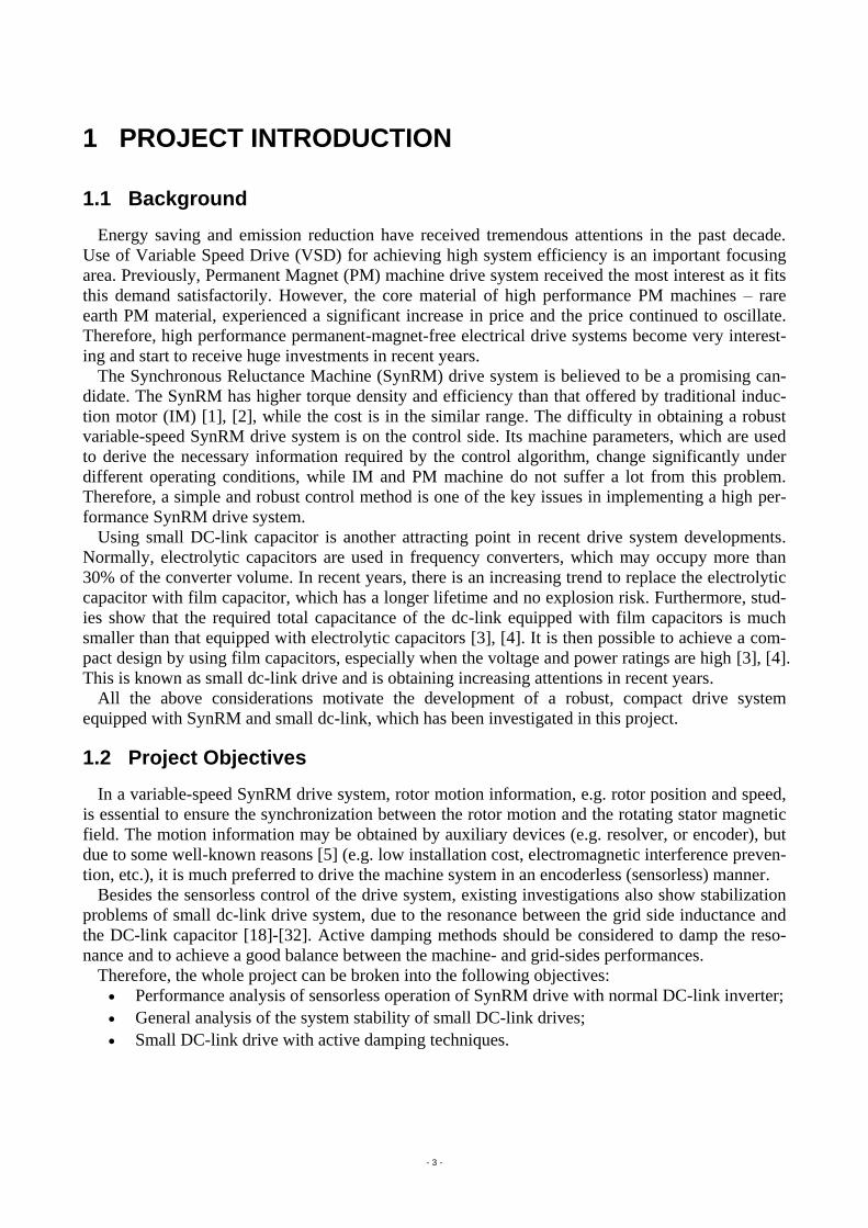
The system setup is shown in Fig. 2.1 and Fig. 2.2. A three-phase frequency converter connected

to the grid is used to drive the SynRM, which is loaded by the load system. The gate signals to the

inverter are provided by the controller. Machine currents and converter dc-link voltage are acquired

by the controller through current and voltage sensors. An encoder is connected to the non-drive-end

of SynRM to provide reference rotor position information. A PC is connected to exchange data and

control signals with the controller.

Controller

as bs cs

ai

bi

ci

r

Three-phase

Voltage

Source

SynRMdcv

Load

System

1i

2i

3i

Rectifier Inverter

Frequency Converter

Encoder

PC

CurrentSensors

Fig. 2.1. Block diagram of the SynRM drive system setup.

(a) (b) .

Fig. 2.2. Pictures of the system setup. (a) Frequency converter. (b) Machine test bench.

2.2 Drive System

2.2.1 Frequency Converter

The 7.5kW (400V) frequency converter accepts input of “3×380-500V, 50/60Hz 14.4/13.0A”,

and the output is “3×0-Vin 0-590Hz 16/14.5A”, where “Vin” means the input voltage of the fre-

quency converter. The type code of the frequency converter used in this project is FC-

302P7K5T5E20H1BGXXXXSXXXXAXBXCXXXXDX, and the power module used in the fre-

quency converter is DP50H1200T101729.

The control panel of the commercial frequency converter is replaced with an interface and protec-

tion card (IPC) as shown in Fig. 2.2 (a), which can receive the control/gate signals from the control-

Encoder SynRM Generator

- 5 -

ler. The inverter dead time can be set by the IPC with the options of 2μs, 2.5μs, 3μs or 4μs. In this

project, 2μs dead time is used.

2.2.2 Synchronous Reluctance Machine

The parameters of the 5.5kW SynRM at rated condition are listed in Table 2.1. Studies have

shown that the machine inductances vary for different load conditions due to the self- and cross-

saturation effects [6]-[7], the d- and q-axes inductances at different load conditions are tested and

shown in Fig. 2.3.

Table 2.1. Parameters of SynRM

Rated power 5.5 kW Rated frequency 50 Hz

Rated voltage 353 V Power factor 0.69

Rated current 13.9 A Stator resistance 0.38 Ω

Rated speed 1500 rpm Inertia 1.9 102 kg·m2

Rated torque 35.0 N·m Pole pairs 2

05

1015 0

510

15

40

45

50

55

40

45

50

Id (A)Iq (A)

05

1015 0

510

15

10

20

30

10

15

20

25

Id (A)Iq (A)

(a) (b)

Fig. 2.3. Machine inductance at different load conditions. (a) d-axis inductance. (b) q-axis inductance.

2.2.3 Sensor Box

The sensor box contains three current transducers (LA 55-P) and one voltage transducers (LV 25-

P).

The measuring resistance of LA 55-P is designed to be about 21.2Ω, so that the output voltage is

in the range of ±1.5V. The number of windings is set to be two, which corresponds to a current

measuring range of ±25A peak.

The measuring resistance of LV 25-P at primary side is designed to be 80kΩ, so that it can meas-

ure up to 800V within primary nominal current limit (10mA). The measuring resistance at the sec-

ondary side is 60Ω to give a ±1.5V voltage output.

2.2.4 Controller

The whole controller includes a digital signal processor (DSP), a USB docking station, and an in-

terface board as shown in Fig. 2.4. The interface board contains the connection ports with other

devices, including encoder, frequency converter, and sensor box. Since the voltage signals from

sensors are at the level of ±1.5V, level shifting circuits are integrated in the interface board to shift

the input voltage to 0-3V, which is required for ADC inputs of DSP.

- 6 -

Fig. 2.4. Controller of the drive system.

2.3 Load System

The load system contains a generator, a three-phase transformer, and a three-phase resistor bank.

A PM machine is used to serve as the generator. The generated three-phase voltage is increased by

the transformer to ensure that the resistor bank can consume enough power even at low speed op-

eration range. The parameters of the PM machine are listed in Table 2.2.

Table 2.2. Parameters of PM Generator

Rated power 6.67 kW Standstill torque 29.4 N·m

Rated torque 18.2 N·m Standstill current 18.7 A

Rated speed 3500 rpm Stator resistance 0.35 Ω

Rated voltage 480 V Inertia 6.5 103 kg·m2

Torque constant 1.58 Pole pairs 5

According to the manual of the PM machine, the standstill torque and current can be maintained

indefinitely at a speed between 0 and 100rpm and rated ambient conditions. However, since it is

only for lab experiments rather than continuous operation, the standstill torque can be achieved

even for speed up to 1500rpm during the test. Therefore, the SynRM can be loaded to about

29.4Nm by the load system, which corresponds to about 12A load current of SynRM.

2.4 Small DC-Link Drive

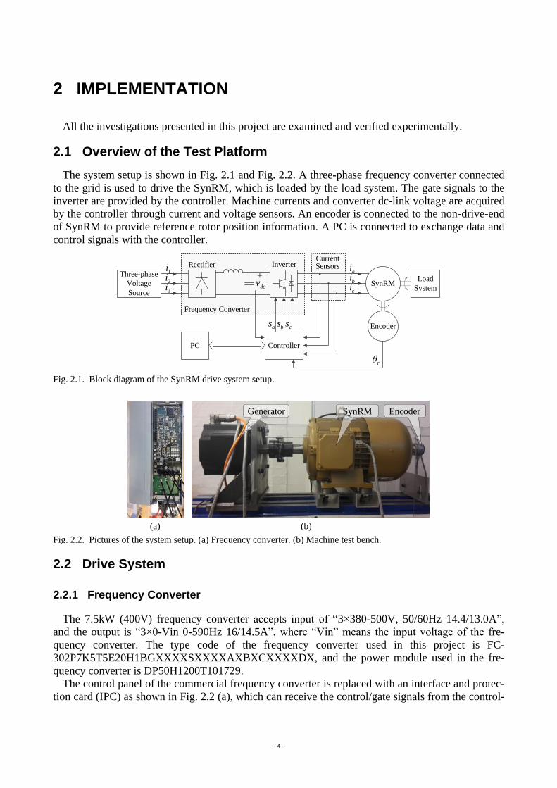
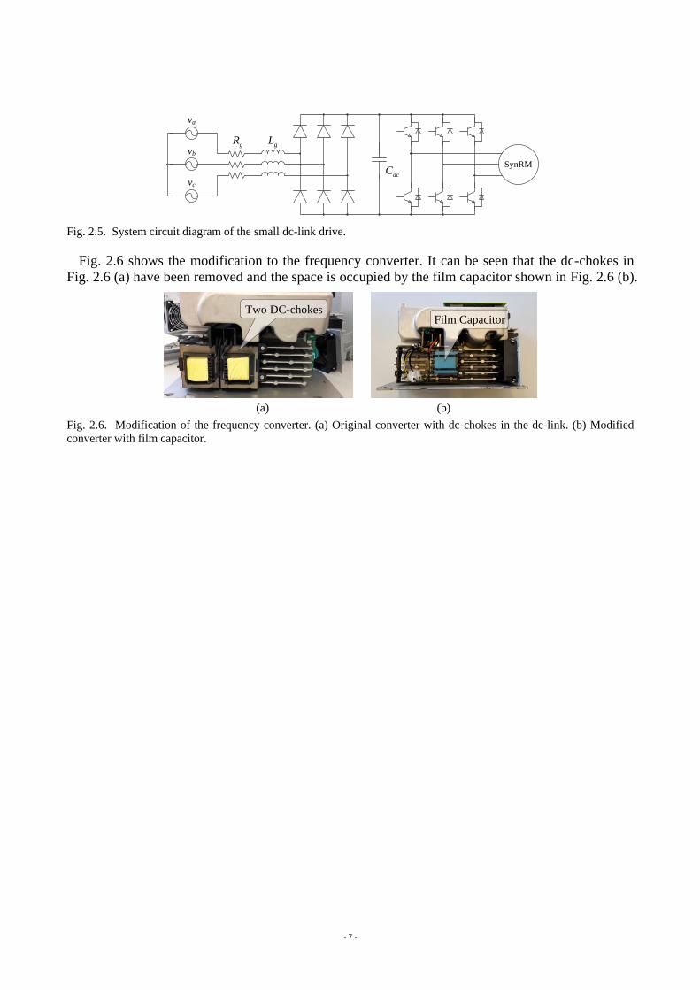
To carry out the studies for small dc-link drive, a 7.5kW Danfoss VLT® AutomationDrive FC

302 frequency converter is modified. The original electrolytic capacitors (two 450V 1000μF con-

nected in series) in the dc-link are replaced with a film capacitor (1200V 14μF), while the dc-

chokes in the dc-link are removed. A three-phase line reactor (31.47mH) is connected between the

grid and the frequency converter to perform the function of dc-chokes as well as the soft grid. The

system circuit diagram of the small dc-link drive is illustrated in Fig. 2.5, where Rg and Lg are grid

resistance and inductance, respectively.

DSP &

Docking station

Interface board

Sensor Inputs Optical Outputs

Optical

Inputs

Encoder

Inputs

Level

Shifting

Circuits

- 7 -

SynRM

va

vb

vc

dcC

gR gL

Fig. 2.5. System circuit diagram of the small dc-link drive.

Fig. 2.6 shows the modification to the frequency converter. It can be seen that the dc-chokes in

Fig. 2.6 (a) have been removed and the space is occupied by the film capacitor shown in Fig. 2.6 (b).

(a) (b) .

Fig. 2.6. Modification of the frequency converter. (a) Original converter with dc-chokes in the dc-link. (b) Modified

converter with film capacitor.

Two DC-chokes Film Capacitor

- 8 -

3 POSITION-SENSORLESS CONTROL

The position-sensorless control of the SynRM drive system equipped with normal DC-link con-

verter is investigated first. The field-oriented control (FOC) together with the space vector modula-

tion (SVM) technology is implemented [8]. Position sensorless control technique based on the ma-

chine fundamental voltage such as electromotive force (EMF) or flux linkage is adopted.

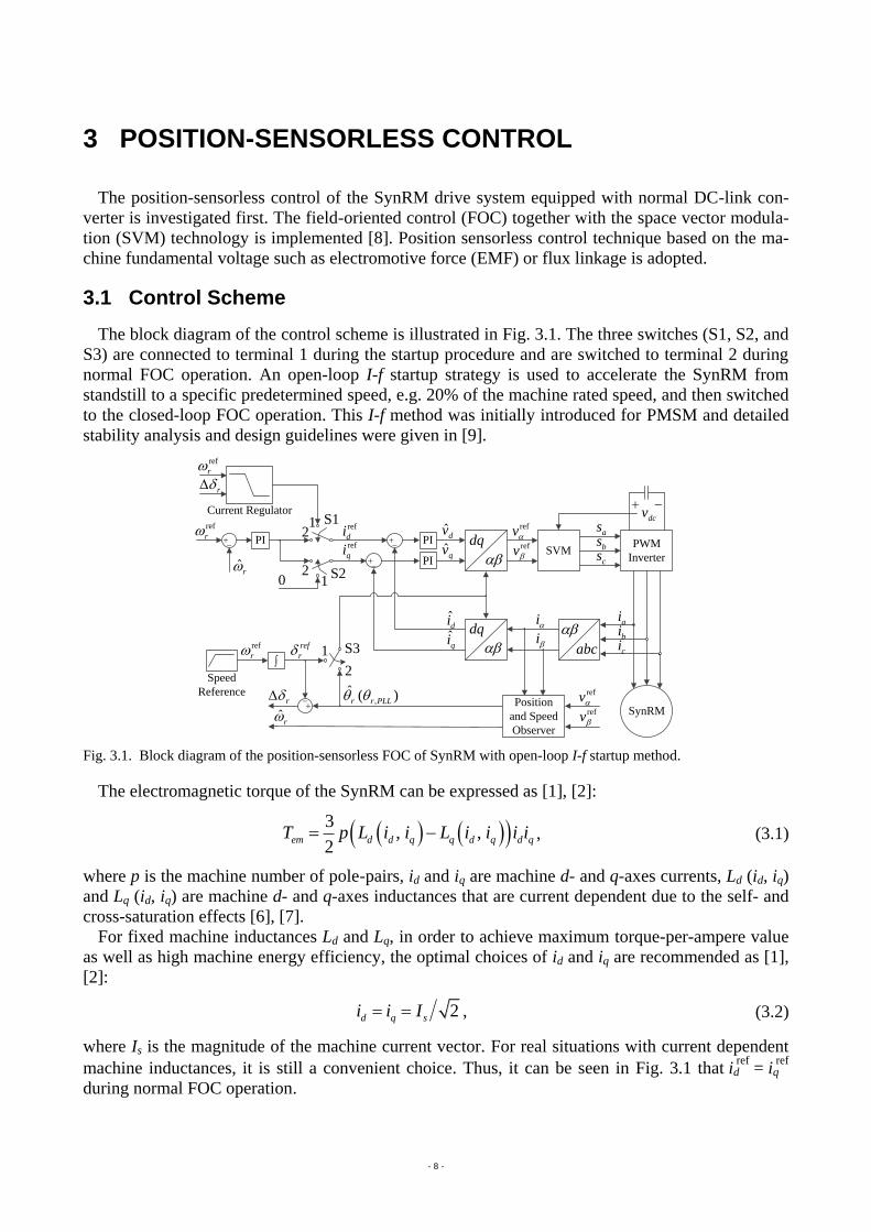
3.1 Control Scheme

The block diagram of the control scheme is illustrated in Fig. 3.1. The three switches (S1, S2, and

S3) are connected to terminal 1 during the startup procedure and are switched to terminal 2 during

normal FOC operation. An open-loop I-f startup strategy is used to accelerate the SynRM from

standstill to a specific predetermined speed, e.g. 20% of the machine rated speed, and then switched

to the closed-loop FOC operation. This I-f method was initially introduced for PMSM and detailed

stability analysis and design guidelines were given in [9].

refvrefv

SVM

dq

SynRM

dq

abc

ai

bi

ci

iiˆ

qi

ˆdi

refvrefv

PI

PIˆ

dv

ˆqv

,ˆ ( )r r PLL

PI

ref

r

0

1

2

∫

ˆr

ref

rref

r

r

2Speed

Reference

ref

r

r

1

21

Current Regulator

as

bs

cs

dcv

PWM

Inverter

ref

diref

qi

S1

S2

S3

Position

and Speed

Observer

ˆr

Fig. 3.1. Block diagram of the position-sensorless FOC of SynRM with open-loop I-f startup method.

The electromagnetic torque of the SynRM can be expressed as [1], [2]:

3

, , 2

em d d q q d q d qT p L i i L i i i i , (3.1)

where p is the machine number of pole-pairs, id and iq are machine d- and q-axes currents, Ld (id, iq)

and Lq (id, iq) are machine d- and q-axes inductances that are current dependent due to the self- and

cross-saturation effects [6], [7].

For fixed machine inductances Ld and Lq, in order to achieve maximum torque-per-ampere value

as well as high machine energy efficiency, the optimal choices of id and iq are recommended as [1],

[2]:

2 d q si i I , (3.2)

where Is is the magnitude of the machine current vector. For real situations with current dependent

machine inductances, it is still a convenient choice. Thus, it can be seen in Fig. 3.1 that idref

= iqref

during normal FOC operation.

- 9 -

3.2 Position and Speed Observer

The conventional machine voltage model represented in the stationary αβ-reference frame can be

expressed as:

s

dv R i

dt , (3.3)

where Rs is the stator phase resistance, vαβ, iαβ, and λαβ are the machine stator voltage vector, current

vector, and flux linkage vector, respectively. Thus, the machine flux linkage vector in the stationary

αβ-reference frame can be calculated as:

sv R i dt . (3.4)

Instead of the integration of the voltage/EMF information in (3.4), the flux linkage can be ob-

tained alternatively from the machine currents and inductances information, which is known as the

machine current model:

r rj j

dq pm d d q qe L i jL i e

, (3.5)

where λpm is the magnitude of the possible rotor PM flux-linkage, and θr is the machine rotor posi-

tion that is aligned with machine d-axis.

It can be obtained from (3.5) that the rotor position θr can be calculated as:

1arg tan

q

r q

q

L iL i

L i

. (3.6)

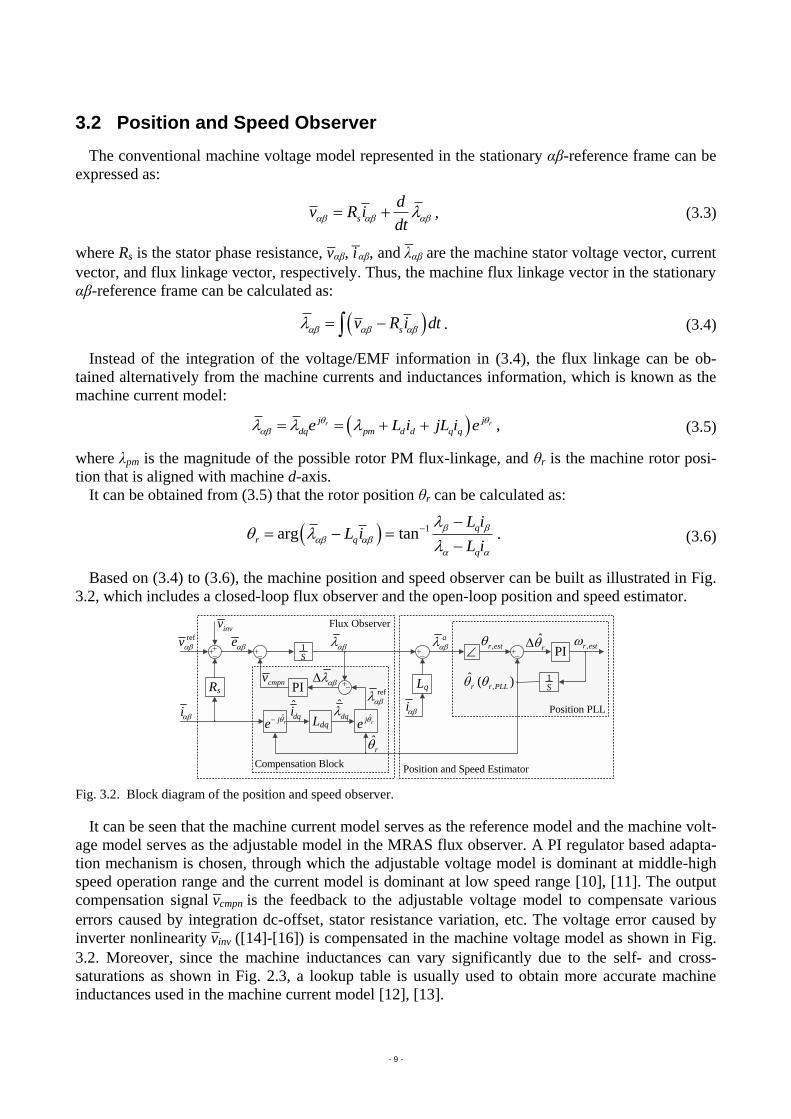
Based on (3.4) to (3.6), the machine position and speed observer can be built as illustrated in Fig.

3.2, which includes a closed-loop flux observer and the open-loop position and speed estimator.

i

refv

Rs

ˆdqi

ˆdq

ref

ˆr

i

,r est

,ˆ ( )r r PLL

ˆ r,r est

Position PLL

Flux Observer

Compensation Block

cmpnv

Position and Speed Estimator

invv

1S

1S

Ldqˆ rj

e ˆ

rje

PI Lq

PI

a

e

Fig. 3.2. Block diagram of the position and speed observer.

It can be seen that the machine current model serves as the reference model and the machine volt-

age model serves as the adjustable model in the MRAS flux observer. A PI regulator based adapta-

tion mechanism is chosen, through which the adjustable voltage model is dominant at middle-high

speed operation range and the current model is dominant at low speed range [10], [11]. The output

compensation signal vcmpn is the feedback to the adjustable voltage model to compensate various

errors caused by integration dc-offset, stator resistance variation, etc. The voltage error caused by

inverter nonlinearity vinv ([14]-[16]) is compensated in the machine voltage model as shown in Fig.

3.2. Moreover, since the machine inductances can vary significantly due to the self- and cross-

saturations as shown in Fig. 2.3, a lookup table is usually used to obtain more accurate machine

inductances used in the machine current model [12], [13].

- 10 -

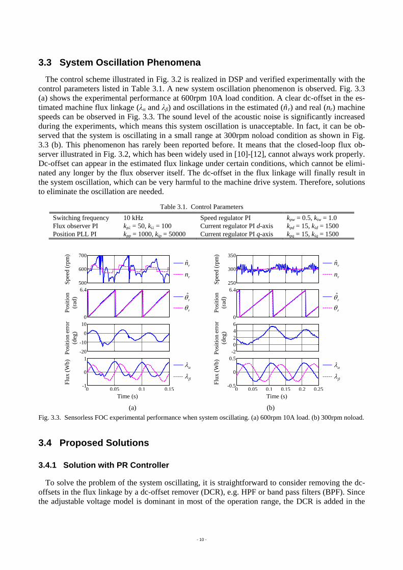
3.3 System Oscillation Phenomena

The control scheme illustrated in Fig. 3.2 is realized in DSP and verified experimentally with the

control parameters listed in Table 3.1. A new system oscillation phenomenon is observed. Fig. 3.3

(a) shows the experimental performance at 600rpm 10A load condition. A clear dc-offset in the es-

timated machine flux linkage (λα and λβ) and oscillations in the estimated (n r) and real (nr) machine

speeds can be observed in Fig. 3.3. The sound level of the acoustic noise is significantly increased

during the experiments, which means this system oscillation is unacceptable. In fact, it can be ob-

served that the system is oscillating in a small range at 300rpm noload condition as shown in Fig.

3.3 (b). This phenomenon has rarely been reported before. It means that the closed-loop flux ob-

server illustrated in Fig. 3.2, which has been widely used in [10]-[12], cannot always work properly.

Dc-offset can appear in the estimated flux linkage under certain conditions, which cannot be elimi-

nated any longer by the flux observer itself. The dc-offset in the flux linkage will finally result in

the system oscillation, which can be very harmful to the machine drive system. Therefore, solutions

to eliminate the oscillation are needed.

Table 3.1. Control Parameters

Switching frequency 10 kHz Speed regulator PI kpw = 0.5, kiw = 1.0

Flux observer PI kpλ = 50, kiλ = 100 Current regulator PI d-axis kpd = 15, kid = 1500

Position PLL PI kpp = 1000, kip = 50000 Current regulator PI q-axis kpq = 15, kiq = 1500

500

600

700

-20

-10

0

10

0 0.05 0.1 0.15-1

0

1

0

6.4

Po

siti

on

(rad

)

Time (s)

Po

siti

on

err

or

(deg

)

Sp

eed

(rp

m)

Flu

x (

Wb

)

rn

ˆrn

r

ˆr

0 0.05 0.1 0.15 0.2 0.25-0.5

0

0.5

250

300

350

0

6.4

-2

0

2

4

6

Po

siti

on

(rad

)

Time (s)

Po

siti

on

err

or

(deg

)

Sp

eed

(rp

m)

Flu

x (

Wb

)

rn

ˆrn

r

ˆr

(a) (b)

Fig. 3.3. Sensorless FOC experimental performance when system oscillating. (a) 600rpm 10A load. (b) 300rpm noload.

3.4 Proposed Solutions

3.4.1 Solution with PR Controller

To solve the problem of the system oscillating, it is straightforward to consider removing the dc-

offsets in the flux linkage by a dc-offset remover (DCR), e.g. HPF or band pass filters (BPF). Since

the adjustable voltage model is dominant in most of the operation range, the DCR is added in the

- 11 -

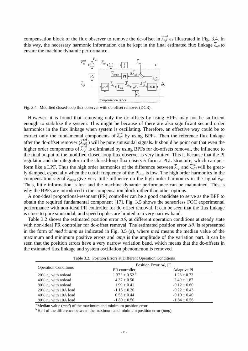
compensation block of the flux observer to remove the dc-offset in λαβ¯

ref as illustrated in Fig. 3.4. In

this way, the necessary harmonic information can be kept in the final estimated flux linkage λαβ to

ensure the machine dynamic performance.

ˆri

refv

Rs

dqi dqref

ˆr

Compensation Block

cmpnv

invv

1S

Ldqˆ rj

e ˆ

rje

PI ref

1

e

DCR

Fig. 3.4. Modified closed-loop flux observer with dc-offset remover (DCR).

However, it is found that removing only the dc-offsets by using HPFs may not be sufficient

enough to stabilize the system. This might be because of there are also significant second order

harmonics in the flux linkage when system is oscillating. Therefore, an effective way could be to

extract only the fundamental components of λαβ¯

ref by using BPFs. Then the reference flux linkage

after the dc-offset remover (λαβ1¯

ref ) will be pure sinusoidal signals. It should be point out that even the

higher order components of λαβ¯

ref is eliminated by using BPFs for dc-offsets removal, the influence to

the final output of the modified closed-loop flux observer is very limited. This is because that the PI

regulator and the integrator in the closed-loop flux observer form a PLL structure, which can per-

form like a LPF. Thus the high order harmonics of the difference between λαβ and λαβ1¯

ref will be great-

ly damped, especially when the cutoff frequency of the PLL is low. The high order harmonics in the

compensation signal vcmpn give very little influence on the high order harmonics in the signal eαβ.

Thus, little information is lost and the machine dynamic performance can be maintained. This is

why the BPFs are introduced in the compensation block rather than other options.

A non-ideal proportional-resonant (PR) controller can be a good candidate to serve as the BPF to

obtain the required fundamental component [17]. Fig. 3.5 shows the sensorless FOC experimental

performance with non-ideal PR controller for dc-offset removal. It can be seen that the flux linkage

is close to pure sinusoidal, and speed ripples are limited to a very narrow band.

Table 3.2 shows the estimated position error Δθr at different operation conditions at steady state

with non-ideal PR controller for dc-offset removal. The estimated position error Δθr is represented

in the form of med ± amp as indicated in Fig. 3.5 (a), where med means the median value of the

maximum and minimum positive errors and amp is the amplitude of the variation part. It can be

seen that the position errors have a very narrow variation band, which means that the dc-offsets in

the estimated flux linkage and system oscillation phenomenon is removed.

Table 3.2. Position Errors at Different Operation Conditions

Operation Conditions Position Error Δθr [˚]

PR controller Adaptive PI

20% nrt with noload 1.37 a ± 0.52 b 1.28 ± 0.72

40% nrt with noload 4.37 ± 0.50 2.40 ± 1.87

80% nrt with noload 1.99 ± 0.41 -0.12 ± 0.60

20% nrt with 10A load -1.15 ± 0.30 -0.22 ± 0.43

40% nrt with 10A load 0.53 ± 0.44 -0.10 ± 0.40

80% nrt with 10A load -1.80 ± 0.50 -1.84 ± 0.56 a Median value (med) of the maximum and minimum position error b Half of the difference between the maximum and minimum position error (amp)

- 12 -

0 0.05 0.1 0.15 0.2 0.25-0.5

0

0.5

290

300

310

0.5

1

1.5

2

Time (s)

Po

siti

on

err

or

(deg

)

Sp

eed

(rp

m)

Flu

x (

Wb

)

rn

ˆrn

max

min

med

amp

590

600

610

0

0.5

1

0 0.05 0.1 0.15-1

0

1

Time (s)

Po

siti

on

err

or

(deg

)

Sp

eed

(rp

m)

Flu

x (

Wb

)

rn

ˆrn

(a) (b)

100

300

500

-20

0

20

40

0 0.5 1 1.5 2-1

0

1

Time (s)

Po

siti

on

err

or

(deg

)

Sp

eed

(rp

m)

Flu

x (

Wb

)

rn

ˆrn

(c)

Fig. 3.5. Sensorless FOC experimental performance with non-ideal PR controller. (a) 300rpm noload. (b) 600rpm

10A load. (c) 12A step load on and off at 300rpm.

3.4.2 Solution with Adaptive PI Controllers

Another possible way to solve the system oscillation is to increase the damping factor of the os-

cillations. It is found that reducing the oscillating components in λ ˆ d and λ ˆ q, which are caused by the

oscillating id and iq, could help to reduce the distortion of λαβ¯

ref. Since id and iq are equal to each other,

and Ld is much larger than Lq, λ ˆ d is dominant in the flux linkage vector. Reducing the oscillation in

id could be considered as a solution. This can be achieved by reducing the PI parameters of the

speed regulator and the d-axis current regulator. The reduced dc-offset in the reference machine

current model will be reflected to the machine voltage model through the compensation block. Be-

sides, further decay and phase delay of the oscillating components may be introduced by the posi-

tion PLL. The decayed position and speed oscillations will be fed back and the system may finally

settle in a steady-state condition where the oscillations are greatly suppressed.

The above idea is implemented in the real system by using the adaptive PI controllers (including

the speed and d-axis current controllers), where the PI parameters are adjusted according to the de-

viation between the estimated speed feedback ωr and the reference speed ωrref

. Small PI parameters

(e.g. kpw = 0.3, kiw = 0.6, kpd = 10, and kid = 100) are used when the difference between ωr and ωrref

are

- 13 -

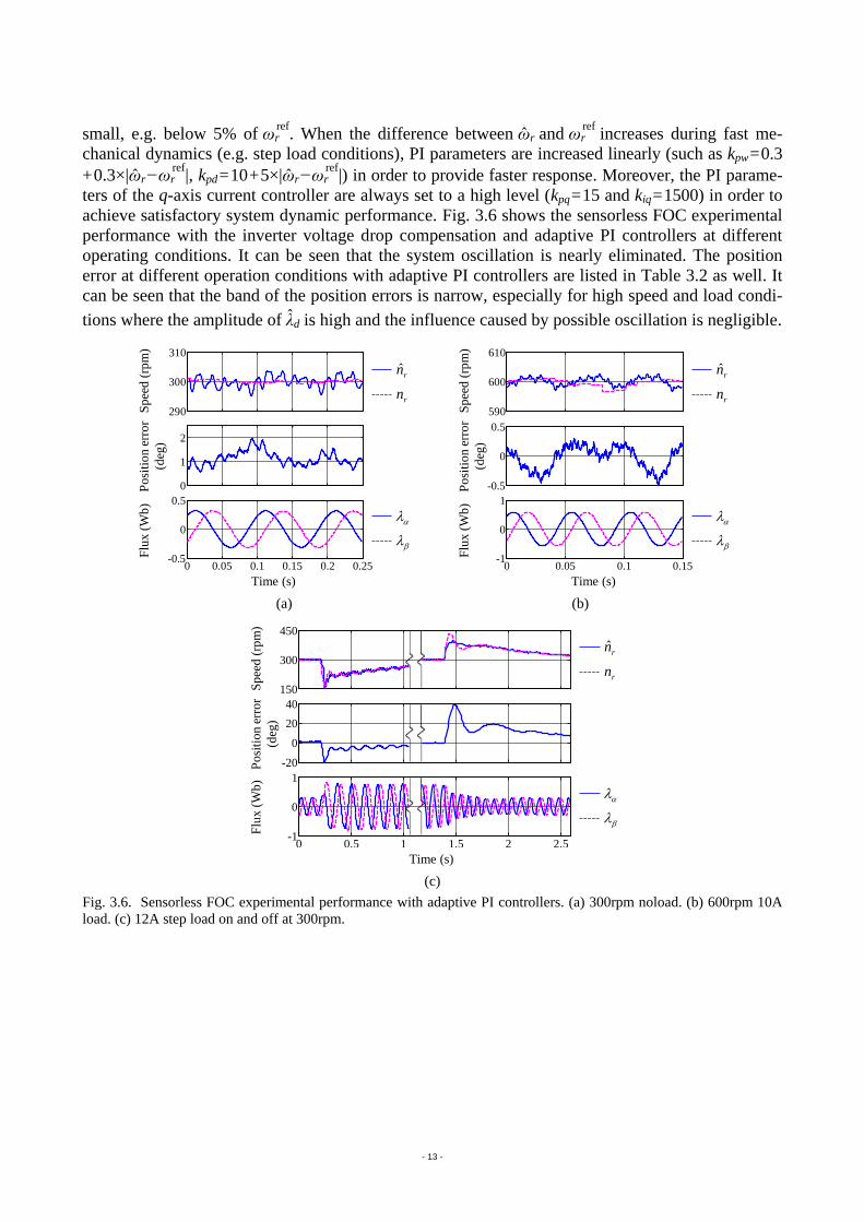
small, e.g. below 5% of ωrref

. When the difference between ωr and ωrref

increases during fast me-

chanical dynamics (e.g. step load conditions), PI parameters are increased linearly (such as kpw = 0.3

+ 0.3×|ωr − ωrref

|, kpd = 10 + 5×|ωr − ωrref

|) in order to provide faster response. Moreover, the PI parame-

ters of the q-axis current controller are always set to a high level (kpq = 15 and kiq = 1500) in order to

achieve satisfactory system dynamic performance. Fig. 3.6 shows the sensorless FOC experimental

performance with the inverter voltage drop compensation and adaptive PI controllers at different

operating conditions. It can be seen that the system oscillation is nearly eliminated. The position

error at different operation conditions with adaptive PI controllers are listed in Table 3.2 as well. It

can be seen that the band of the position errors is narrow, especially for high speed and load condi-

tions where the amplitude of λ ˆ d is high and the influence caused by possible oscillation is negligible.

290

300

310

0

1

2

0 0.05 0.1 0.15 0.2 0.25-0.5

0

0.5

Time (s)

Po

siti

on

err

or

(deg

)

Sp

eed

(rp

m)

Flu

x (

Wb

)

rn

ˆrn

590

600

610

-0.5

0

0.5

0 0.05 0.1 0.15-1

0

1

Time (s)

Po

siti

on

err

or

(deg

)

Sp

eed

(rp

m)

Flu

x (

Wb

)

rn

ˆrn

(a) (b)

-20

0

20

40

150

300

450

0 0.5 1 1.5 2 2.5-1

0

1

Time (s)

Po

siti

on

err

or

(deg

)

Sp

eed

(rp

m)

Flu

x (

Wb

)

rn

ˆrn

(c)

Fig. 3.6. Sensorless FOC experimental performance with adaptive PI controllers. (a) 300rpm noload. (b) 600rpm 10A

load. (c) 12A step load on and off at 300rpm.

- 14 -

3.5 Summary

The position estimation algorithm via flux linkage is carried out and has been fully tested.

Though the closed-loop flux observer is widely used in various types of machine drives and can

provide satisfactory performance, it is found that it cannot always work properly, especially at the

condition where the magnitude of the flux linkage vector is low and ambiguous compared to the

error- or noise- signals. The compensation block in the closed-loop flux observer may fail in remov-

ing the dc-offset, and system oscillation phenomenon may then occur. Solutions to cope with this

oscillation phenomenon are proposed to eliminate or suppress this harmful system oscillation. The

experimental verifications show that satisfactory performances can be achieved by using the pro-

posed solutions.

- 15 -

4 SMALL DC-LINK SYSTEM ANALYSIS

The characteristics of the small dc-link drive are analyzed, which provides a solid theory funda-

tion for further investigations.

4.1 System Analysis

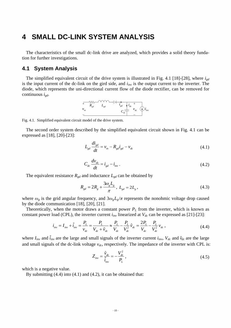
The simplified equivalent circuit of the drive system is illustrated in Fig. 4.1 [18]-[28], where igd

is the input current of the dc-link on the gird side, and iinv is the output current to the inverter. The

diode, which represents the uni-directional current flow of the diode rectifier, can be removed for

continuous igd.

dcC

gdL

inv

gdR gdidci

invidcv

Fig. 4.1. Simplified equivalent circuit model of the drive system.

The second order system described by the simplified equivalent circuit shown in Fig. 4.1 can be

expressed as [18], [20]-[23]:

gd

gd in gd gd dc

diL v R i v

dt (4.1)

dcdc gd inv

dvC i i

dt. . (4.2)

The equivalent resistance Rgd and inductance Lgd can be obtained by

32

g g

gd g

LR R

, 2gd gL L , (4.3)

where ωg is the grid angular frequency, and 3ωg Lg /π represents the nonohmic voltage drop caused

by the diode communication [18], [20], [21].

Theoretically, when the motor draws a constant power PL from the inverter, which is known as

constant power load (CPL), the inverter current iinv linearized at Vdc can be expressed as [21]-[23]:

2 2

2

L L L L L Linv inv inv dc dc

dc dc dc dc dc dc dc

P P P P P Pi I i v v

v V v V V V V, (4.4)

where Iinv and iinv are the large and small signals of the inverter current iinv, Vdc and vdc are the large

and small signals of the dc-link voltage vdc, respectively. The impedance of the inverter with CPL is:

2

dc dcinv

inv L

v VZ

i P, (4.5)

which is a negative value.

By submitting (4.4) into (4.1) and (4.2), it can be obtained that:

- 16 -

2

2 2 2

1 11

gd gd Ldc L dcdc in

gd dc dc gd dc dc gd dc

R R Pd v P dvv v

dt L C V dt L C V L C. (4.6)

The following characteristic equation of the second order system in Laplace domain can be ob-

tained [21]-[24]:

2

2 2

2010

11 0

gd gd LL

gd dc dc gd dc dc

R R PPs s

L C V L C V

aa

. (4.7)

According to Routh-Hurwitz stability criterion, the system is stable when a10 and a20 are greater

than zero. Normally, |Zinv| is much greater than Rgd, i.e. a20 is greater than zero. Then, the system

stability is depending on a10.The system is stable if a10 > 0, i.e.

2 2

gd gdL dc

gd dc dc L gd dc

R LP C

L C V P R V. (4.8)

The system is stable when the criterion of (4.8) is satisfied, which is the condition for normal fre-

quency converters with large electrolytic capacitors. However, it may be not true for small dc-link

drives. When the criterion of (4.8) is not satisfied, the dc-link voltage and grid currents will become

unstable or oscillating [23]-[25]. The overvoltage may destroy the IGBTs and capacitors, and the

lifetime of the capacitor will be reduced due to the voltage oscillation.

The angular frequency of the dc-link voltage oscillation can be calculated analytically according

to the system characteristic equation (4.7). And it can be approximated by the angular resonant fre-

quency of the LC circuit shown in Fig. 4.1, i.e. 1/(Lgd Cdc)1/2

[19]-[21].

4.2 System Performance

For a 50Hz 380V supply and a 5.5kW SynRM load, the capacitance needed to operate the system

stably during the whole power range is about 126μF according to (4.8). The modified small dc-link

drive described in section 2.4 has only 14μF dc-link capacitance, which means that the system may

become unstable when the load increases to a certain level.

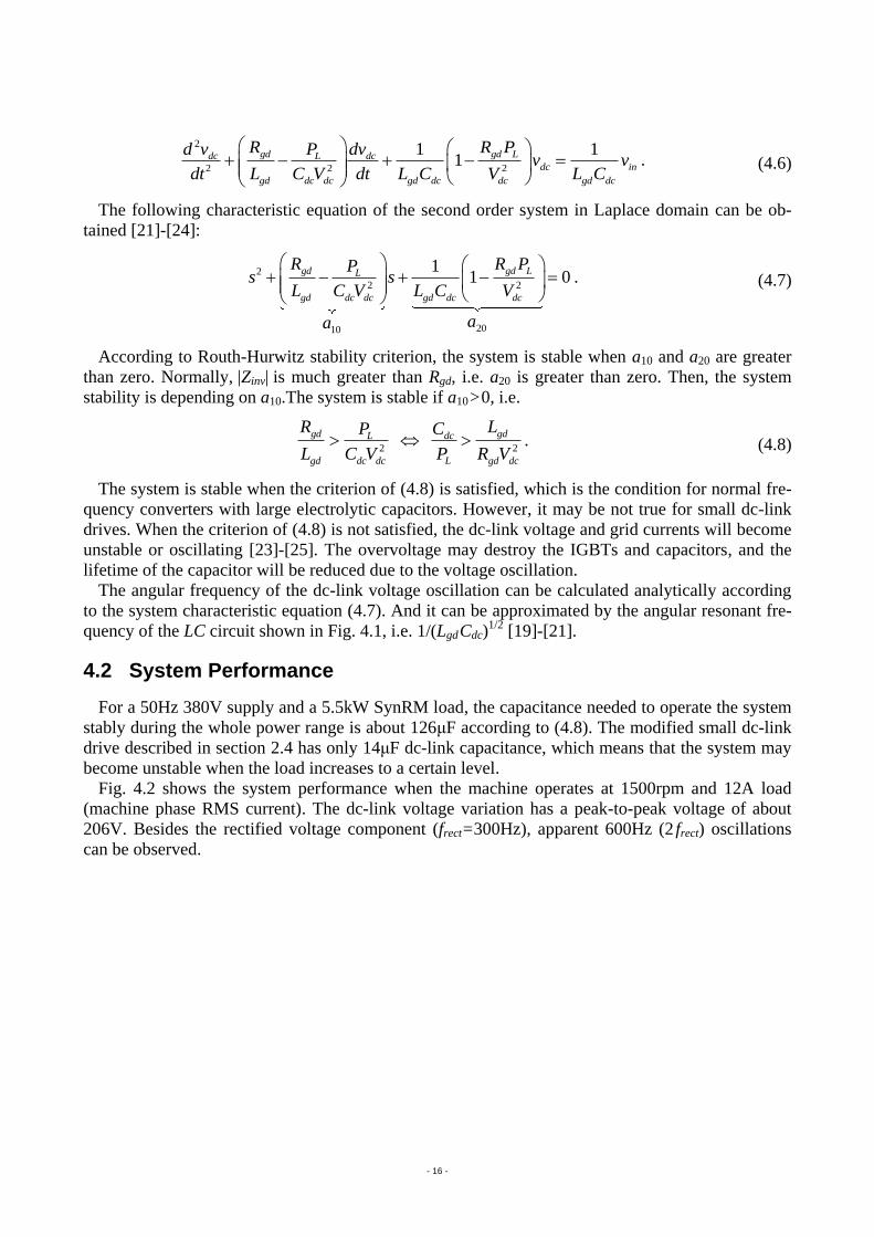
Fig. 4.2 shows the system performance when the machine operates at 1500rpm and 12A load

(machine phase RMS current). The dc-link voltage variation has a peak-to-peak voltage of about

206V. Besides the rectified voltage component (frect=300Hz), apparent 600Hz (2 frect) oscillations

can be observed.

- 17 -

Gri

d

Cu

rren

t (A

)

Time (s)

Mac

hin

e

Cu

rren

t (A

)

DC

-lin

k

Vo

ltag

e (V

)

-10

0

10

0 0.01 0.02 0.03 0.04-20

0

20

400

500

600

0

50

50 300 600 9000

10

20

0

5

Frequency (Hz)

(a) (b)

Fig. 4.2. Small dc-link drive system experimental results at 1500rpm 12A load without active damping control. (a)

Waveforms. (b) Spectrum without dc component.

The total harmonic distortion (THD) and the partially weighted harmonic distortion (PWHD) [29]

of the grid current are 69.0% and 67.0%, respectively. The machine current THD is 3.7%.

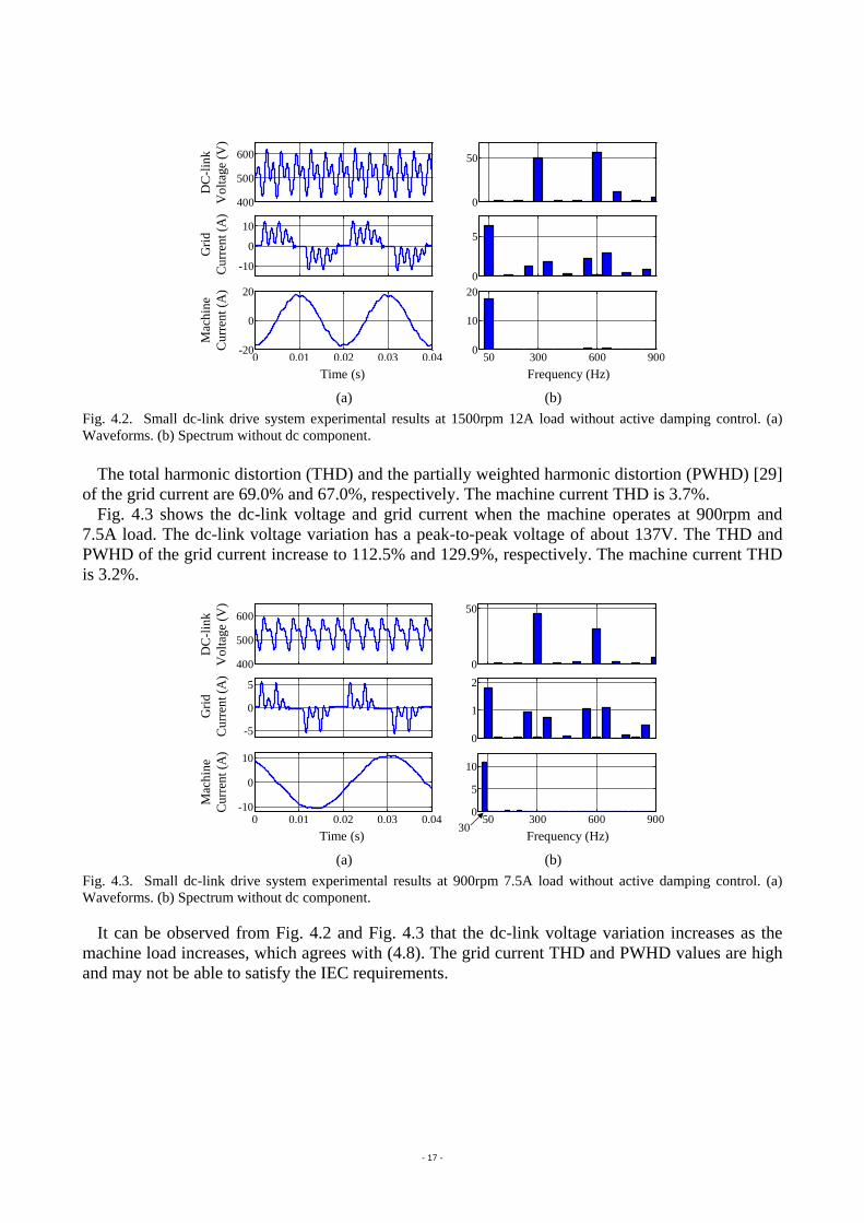
Fig. 4.3 shows the dc-link voltage and grid current when the machine operates at 900rpm and

7.5A load. The dc-link voltage variation has a peak-to-peak voltage of about 137V. The THD and

PWHD of the grid current increase to 112.5% and 129.9%, respectively. The machine current THD

is 3.2%.

50 300 600 9000

5

10

400

500

600

-5

0

5

0

50

0

1

2

0 0.01 0.02 0.03 0.04-10

0

10

Gri

d

Cu

rren

t (A

)

Time (s)

Mac

hin

e

Cu

rren

t (A

)

DC

-lin

k

Vo

ltag

e (V

)

Frequency (Hz)30

(a) (b)

Fig. 4.3. Small dc-link drive system experimental results at 900rpm 7.5A load without active damping control. (a)

Waveforms. (b) Spectrum without dc component.

It can be observed from Fig. 4.2 and Fig. 4.3 that the dc-link voltage variation increases as the

machine load increases, which agrees with (4.8). The grid current THD and PWHD values are high

and may not be able to satisfy the IEC requirements.

- 18 -

4.3 Summary

The small dc-link drive system is analyzed. It is shown that the reduced dc-link capacitance of the

small dc-link drive may result in dc-link voltage oscillation, which is harmful to the drive system

and will reduce the service lifetime. Moreover, the grid current with amplified higher order harmon-

ics around the resonant frequency may fail to meet the requirements from the standards/regulations.

Therefore, techniques to stabilize the dc-link voltage are required, so that the system performance

can meet the expectations.

- 19 -

5 ACTIVE DAMPING METHODS

It has been shown in (4.5) that the inverter has a “negative impedance” characteristic under CPL

condition, and its absolute value increases as the load increases. The whole system will become

unstable when the load increases to a certain level and the damping factor of the system characteris-

tic equation (4.7) reduces to a negative value. The basic idea of active damping methods is to

achieve positive dynamic damping factor by controlling the actual power drawn by the machine

from the dc-link [18]-[28]. As the machine input power is no longer constant, machine torque ripple

will appear and it is only suitable for applications with moderate machine shaft dynamic require-

ments. However, as no extra damping circuit is required, it is a cheap solution and is adopted in this

project.

5.1 Active Damping Methods

5.1.1 Current Injection Active Damping Control

It is straight forward to control the power drawn by the machine by controlling the torque produc-

ing current component directly. Different methods to obtain the proper current reference were pro-

posed [21], [24]-[27]. Taking the method in [21] as an example, a term proportional to the dc-link

voltage variation term vdc, i.e. the small signal of dc-link voltage, is added/injected to the torque

producing current reference iqref

, which can be expressed as:

ref ref ref ref

q q q q iq dci I i I g v . (5.1)

where Iqref

is the unmodified component, i.e. large signal of iqref

for steady state operating conditions,

and giq is the gain factor of q-axis injected current term. Similarly, a gain factor gid can be intro-

duced to control the current term injected to d-axis.

Then, iinv linearized at Vdc can be calculated as:

2 2

3( ) ( ) ,2

q iqL L L L

inv dc dc

dc dc dc dc dc

V gP P P Pi v g v

V V V V V (5.2)

when vdc/Vdc approaches zero.

By submitting (5.2) into (4.1) and (4.2), the following characteristic equation of the second order

system in the Laplace variable s can be obtained:

2

2 2

2111

1 1( ) 1 ( ) 0

gd L Lgd

gd dc dc gd dc dc

R P Ps g s R g

L C V L C V

aa

. (5.3)

Compared with the original system characteristic equation (4.7), a new term g is introduced in

(5.3) when injecting a variation term iqref

. It can be easily found that when

2 L dcg P V , (5.4)

a11 and a21 will be greater than zero and the system is stable according to Routh-Hurwitz stability

criterion. Similar criterion can be obtained by repeating the above analysis when injecting in d-axis

current reference.

- 20 -

5.1.2 Voltage Injection Active Damping Control

In a real digital control system, it is not easy to achieve ideal current injection due to the band-

width limitation. Thus, instead of controlling the current reference, active damping methods based

on the reference voltage control are suggested [18]-[20], [22], [23], [28].

Similarly as the above current injection method, voltage variation terms vd and vq are injected into

the machine dq-axes stator voltages to achieve positive dynamic damping factor. The voltage varia-

tions terms are defined as [18]:

d vd dcv g v and q vq dcv g v , (5.5)

where gvd and gvq are the gain factors of d- and q-axes injected voltage terms, respectively.

When vdc/Vdc approaches zero, iinv can be calculated as:

2 2

3( ) ( ) .2

d vd q vqL L L Linv dc dc

dc dc dc dc dc

I g I gP P P Pi v g v

V V V V V (5.6)

It can be observed that (5.6) has the same form as (5.2). The system characteristic equation iden-

tical to (5.3) will be obtained. The same stability criterion (5.4) would be achieved as well.

5.1.3 Virtual Positive Impedance Active Damping Method

The system analysis showed that the “negative impedance” characteristic of the inverter at CPL

condition is the root cause of the system instability. Therefore, the system can be stabilized if the

“negative impedance” characteristic can be manipulated to perform like positive impedance. The

“virtual positive impedance” active damping method is based on such an idea [22].

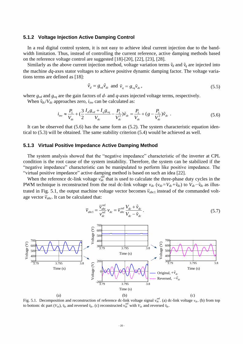
When the reference dc-link voltage vdcref

that is used to calculate the three-phase duty cycles in the

PWM technique is reconstructed from the real dc-link voltage vdc (vdc = Vdc + vdc) to Vdc − vdc as illus-

trated in Fig. 5.1, the output machine voltage vector becomes vabc1 instead of the commanded volt-

age vector vabc. It can be calculated that:

refref

1 ref

abc dc dcabc dc abc

dc dc dc

v V vv v v

v V v. (5.7)

3.79 3.795 3.8300

400

500

600

700

3.79 3.795 3.8300

400

500

600

700

3.79 3.795 3.8-200

0

2003.79 3.795 3.8

300

400

500

600

700

Time (s)

Vo

ltag

e (V

)

Time (s)

Vo

ltag

e (V

)

Time (s)

Vo

ltag

e (V

)

Original,

Reversed,

Time (s)

Vo

ltag

e (V

)

dcv

dcv

(a) (b) (c)

Fig. 5.1. Decomposition and reconstruction of reference dc-link voltage signal vdcref

. (a) dc-link voltage vdc. (b) from top

to bottom: dc part (Vdc), vdc and reversed vdc. (c) reconstructed vdcref

with Vdc and reversed vdc.

- 21 -

The inverter input current iinv can then be calculated and linearized as:

2 2

1

dc dc L L L Linv inv inv L dc dc

dc dc dc dc dc dc dc dc dc

V v P P P Pi I i P v v

V v V v V v V V V. (5.8)

Compared with (4.4), it can be seen that the only difference of (5.8) is that the sign of vdc or vdc is

changed, i.e. the impedance now becomes positive. The system characteristic equation can then be

expressed as:

2

2 2

2212

11 0

gd gd LL

gd dc dc gd dc dc

R R PPs s

L C V L C V

aa

. (5.9)

It can be seen that the coefficients a12 and a22 in (5.9) are always greater than zero and the system

is always stable now. Therefore, instead of finding the gain of variation terms, which are system

parameters and operating condition dependent, the system can be stabilized by simply reconstruct-

ing vdcref

with reversed vdc, and a “virtual positive impedance” characteristic can be obtained. Detailed

analysis shows that the influence of the “virtual positive impedance” active damping method to the

machine variables is equivalent to the q-axis injection.

Furthermore, a factor gv is introduced to control the deviation between reconstructed vdcref

and vdc,

i.e vdcref

= Vdc − gv vdc, (5.9) now become:

2

2 2

2313

11 0

gd v gd Lv L

gd dc dc gd dc dc

R g R Pg Ps s

L C V L C V

aa

. (5.10)

The coefficients a13 and a23 in (5.10) are always greater than zero when gv ≥ 0. It can be observed

that a stable system can already be achieved when gv = 0, i.e. using Vdc to serve as vdcref

is sufficient

enough to stabilize the system. However, the damping factor of (5.10) can be increased by increas-

ing gv, so that the variation terms such as vdc can be suppressed further. But the machine torque rip-

ple will be increased as more oscillating energy is injected into the machine side.

In order to make a clear relation between the meaning and value of the gain factor, a new gain

factor gv0 is introduced, which is defined as:

0 1 v vg g . (5.11)

Then, gv0 = 0 means no active damping is applied, since gv = −1 and vdcref

= vdc. When gv0 ≠ 0, the de-

viation between reconstructed vdcref

and vdc is gv0 vdc. The reverse operation illustrated in Fig. 5.1 cor-

responds to gv0 = 2.

5.2 Verifications

5.2.1 Obtaining DC-Link Voltage Variation

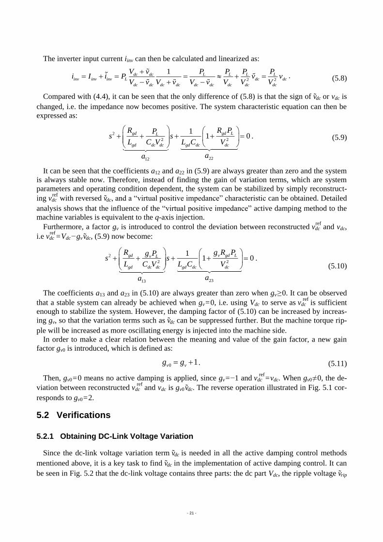
Since the dc-link voltage variation term vdc is needed in all the active damping control methods

mentioned above, it is a key task to find vdc in the implementation of active damping control. It can

be seen in Fig. 5.2 that the dc-link voltage contains three parts: the dc part Vdc, the ripple voltage vrip

- 22 -

at rectified voltage frequency frect, and the oscillating term vosci with frequency fosci. It should be not-

ed that vrip is approaching to the rectified voltage variation term vrect as the load increases when the

Cdc is small.

3.785 3.79 3.795 3.8

-50

0

50

-60

-40

-20

0

20

514

516

518

Time (s)

3.785 3.79 3.795 3.8

500

600

Vo

ltag

e (V

)

Time (s)

dcV

ripv

rectv

osciv

(a) (b)

Fig. 5.2. Composition of the dc-link voltage. (a) dc-link voltage vdc. (b )Top: dc part Vdc; middle: dc-link ripple voltage

vrip and rectified component vrect; bottom: dc-link voltage oscillating term vosci.

There are briefly two ways to define the dc-link voltage variation term vdc. One way is:

dc dc dc rip osciv v V v v . (5.12)

It is the simplest way as Vdc can simply be obtained by using a LPF. However, since vrip is includ-

ed in vdc, the active damping method will try to damp it as well. For machine drive system, this will

result in large machine current ripple at rectified voltage frequency frect. Large torque ripple at the

same frequency will be generated, which may reduce the bearing lifetime and increase the machine

noise level. Therefore, instead of damping both vrip and vosci, it is a better choice to damp vosci only,

i.e. vdc can be defined as:

dc osci dc dc ripv v v V v . (5.13)

It is not an easy task to find vrip from vdc. However, due to the fact that the dc-link ripple voltage

vrip is close to the rectified component vrect at heavy load conditions for small dc-link drive, vrect can

be used to simulate vrip. A complicate method based on PLL and FLL trackers is introduced in [33],

which can calculate Vrect (Vdc + vrect) from vdc by identifying the amplitude, frequency, and phase

angle of Vrect. But the error increases as the load decreases. An alternative method is to use the fun-

damental component of vrip, which is a pure sinusoidal signal at frequency frect, to approximate vrip

[22]. This fundamental component vrip1 can be simply obtained by using a BPF, such as a PR con-

troller [17].

5.2.2 Control Scheme

The control scheme of the small dc-link drive system with active damping control is illustrated in

Fig. 5.3. The “variation detection” block is used to obtain vdc and vdc0. The symbol vdc0, which can

be obtained as vdc0 = vdc − vdc, represents the part of dc-link voltage that will not be damped by the

active damping methods. While flag krip is introduced to control whether the fundamental compo-

- 23 -

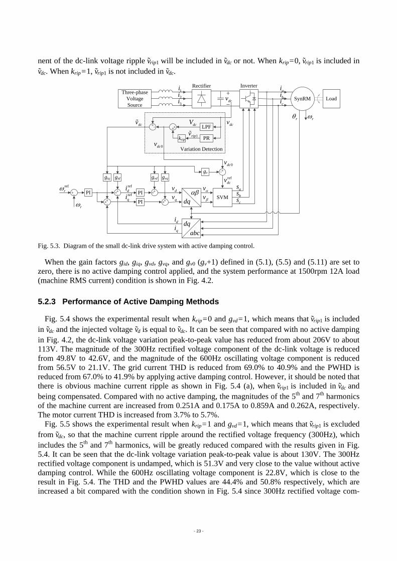
nent of the dc-link voltage ripple vrip1 will be included in vdc or not. When krip = 0, vrip1 is included in

vdc. When krip = 1, vrip1 is not included in vdc.

ref

di vv SVM

ai

bi

ci

qidi

ref

qidv

qvPI

ref

r

r

abc

dq

r

PI

PI

Three-phase

Voltage

Source

SynRM

r

dcv

Load

1i

2i

3i

Rectifier Inverter

LPFdcV

dcv

PR1ripv

dcv

krip

dq

gvd gvqgidgiq

as

bs

cs

0dcvVariation Detection

ref

dcv

gv

0dcv

Fig. 5.3. Diagram of the small dc-link drive system with active damping control.

When the gain factors gid, giq, gvd, gvq, and gv0 (gv+1) defined in (5.1), (5.5) and (5.11) are set to

zero, there is no active damping control applied, and the system performance at 1500rpm 12A load

(machine RMS current) condition is shown in Fig. 4.2.

5.2.3 Performance of Active Damping Methods

Fig. 5.4 shows the experimental result when krip = 0 and gvd = 1, which means that vrip1 is included

in vdc and the injected voltage vd is equal to vdc. It can be seen that compared with no active damping

in Fig. 4.2, the dc-link voltage variation peak-to-peak value has reduced from about 206V to about

113V. The magnitude of the 300Hz rectified voltage component of the dc-link voltage is reduced

from 49.8V to 42.6V, and the magnitude of the 600Hz oscillating voltage component is reduced

from 56.5V to 21.1V. The grid current THD is reduced from 69.0% to 40.9% and the PWHD is

reduced from 67.0% to 41.9% by applying active damping control. However, it should be noted that

there is obvious machine current ripple as shown in Fig. 5.4 (a), when vrip1 is included in vdc and

being compensated. Compared with no active damping, the magnitudes of the 5th

and 7th

harmonics

of the machine current are increased from 0.251A and 0.175A to 0.859A and 0.262A, respectively.

The motor current THD is increased from 3.7% to 5.7%.

Fig. 5.5 shows the experimental result when krip = 1 and gvd = 1, which means that vrip1 is excluded

from vdc, so that the machine current ripple around the rectified voltage frequency (300Hz), which

includes the 5th

and 7th

harmonics, will be greatly reduced compared with the results given in Fig.

5.4. It can be seen that the dc-link voltage variation peak-to-peak value is about 130V. The 300Hz

rectified voltage component is undamped, which is 51.3V and very close to the value without active

damping control. While the 600Hz oscillating voltage component is 22.8V, which is close to the

result in Fig. 5.4. The THD and the PWHD values are 44.4% and 50.8% respectively, which are

increased a bit compared with the condition shown in Fig. 5.4 since 300Hz rectified voltage com-

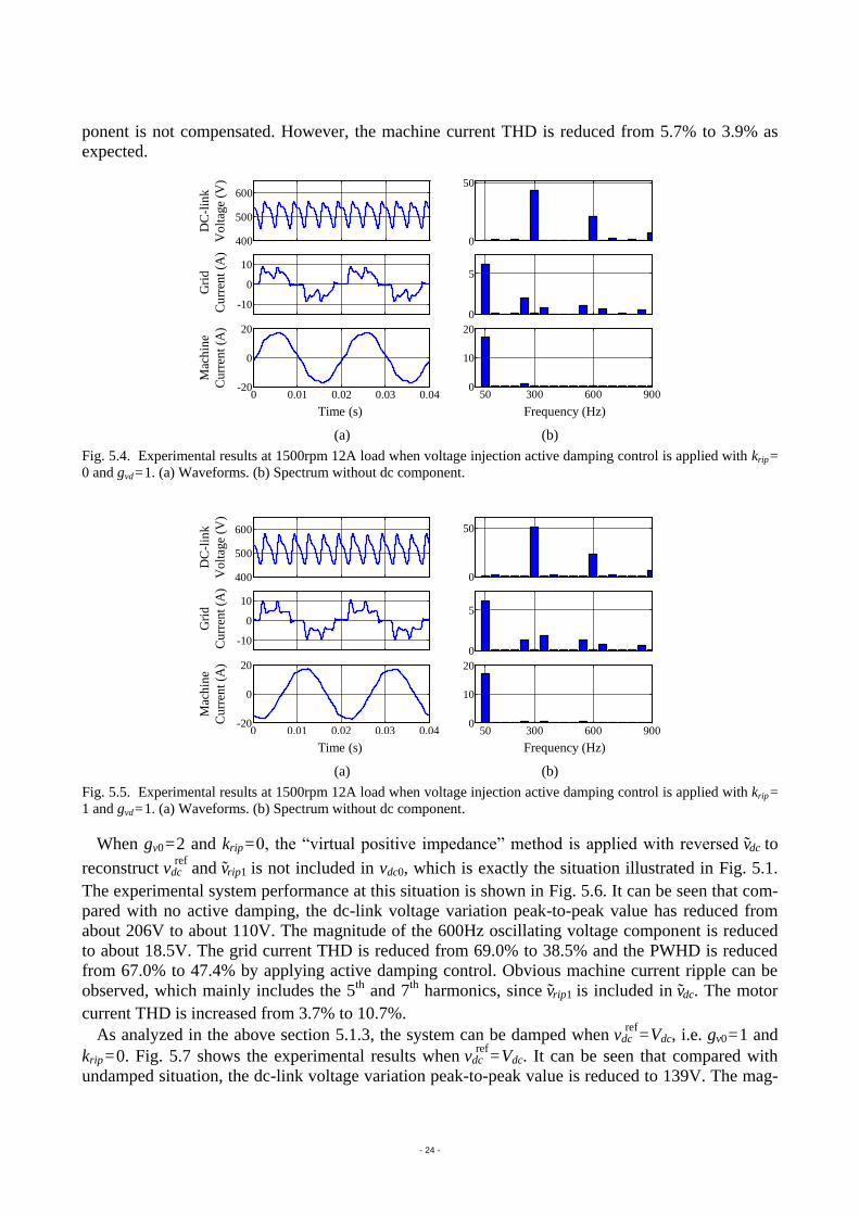
- 24 -

ponent is not compensated. However, the machine current THD is reduced from 5.7% to 3.9% as

expected.

0

50

0

5

50 300 600 9000

10

20

400

500

600

-10

0

10

0 0.01 0.02 0.03 0.04-20

0

20

Gri

d

Cu

rren

t (A

)

Time (s)

Mac

hin

e

Cu

rren

t (A

)

DC

-lin

k

Vo

ltag

e (V

)

Frequency (Hz)

(a) (b)

Fig. 5.4. Experimental results at 1500rpm 12A load when voltage injection active damping control is applied with krip =

0 and gvd = 1. (a) Waveforms. (b) Spectrum without dc component.

0

50

0

5

50 300 600 9000

10

20

400

500

600

-10

0

10

0 0.01 0.02 0.03 0.04-20

0

20

Gri

d

Cu

rren

t (A

)

Time (s)

Mac

hin

e

Cu

rren

t (A

)

DC

-lin

k

Vo

ltag

e (V

)

Frequency (Hz)

(a) (b)

Fig. 5.5. Experimental results at 1500rpm 12A load when voltage injection active damping control is applied with krip =

1 and gvd = 1. (a) Waveforms. (b) Spectrum without dc component.

When gv0 = 2 and krip = 0, the “virtual positive impedance” method is applied with reversed vdc to

reconstruct vdcref

and vrip1 is not included in vdc0, which is exactly the situation illustrated in Fig. 5.1.

The experimental system performance at this situation is shown in Fig. 5.6. It can be seen that com-

pared with no active damping, the dc-link voltage variation peak-to-peak value has reduced from

about 206V to about 110V. The magnitude of the 600Hz oscillating voltage component is reduced

to about 18.5V. The grid current THD is reduced from 69.0% to 38.5% and the PWHD is reduced

from 67.0% to 47.4% by applying active damping control. Obvious machine current ripple can be

observed, which mainly includes the 5th

and 7th

harmonics, since vrip1 is included in vdc. The motor

current THD is increased from 3.7% to 10.7%.

As analyzed in the above section 5.1.3, the system can be damped when vdcref

= Vdc, i.e. gv0 = 1 and

krip = 0. Fig. 5.7 shows the experimental results when vdcref

= Vdc. It can be seen that compared with

undamped situation, the dc-link voltage variation peak-to-peak value is reduced to 139V. The mag-

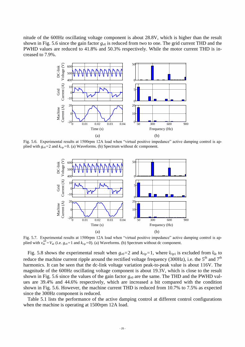
- 25 -

nitude of the 600Hz oscillating voltage component is about 28.8V, which is higher than the result

shown in Fig. 5.6 since the gain factor gv0 is reduced from two to one. The grid current THD and the

PWHD values are reduced to 41.8% and 50.3% respectively. While the motor current THD is in-

creased to 7.9%.

400

500

600

-10

0

10

0 0.01 0.02 0.03 0.04-20

0

20

0

50

0

5

50 300 600 9000

10

20

Gri

d

Cu

rren

t (A

)

Time (s)

Mac

hin

e

Cu

rren

t (A

)

DC

-lin

k

Vo

ltag

e (V

)

Frequency (Hz)

(a) (b)

Fig. 5.6. Experimental results at 1500rpm 12A load when “virtual positive impedance” active damping control is ap-

plied with gv0 = 2 and krip = 0. (a) Waveforms. (b) Spectrum without dc component.

400

500

600

-10

0

10

0 0.01 0.02 0.03 0.04-20

0

20

0

50

0

5

50 300 600 9000

10

20

Gri

d

Cu

rren

t (A

)

Time (s)

Mac

hin

e

Cu

rren

t (A

)

DC

-lin

k

Vo

ltag

e (V

)

Frequency (Hz)

(a) (b)

Fig. 5.7. Experimental results at 1500rpm 12A load when “virtual positive impedance” active damping control is ap-

plied with vdcref

= Vdc (i.e. gv0 = 1 and krip = 0). (a) Waveforms. (b) Spectrum without dc component.

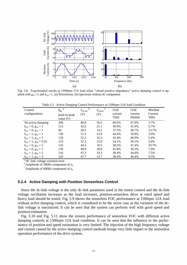
Fig. 5.8 shows the experimental result when gv0 = 2 and krip = 1, where vrip1 is excluded from vdc to

reduce the machine current ripple around the rectified voltage frequency (300Hz), i.e. the 5th

and 7th

harmonics. It can be seen that the dc-link voltage variation peak-to-peak value is about 116V. The

magnitude of the 600Hz oscillating voltage component is about 19.3V, which is close to the result

shown in Fig. 5.6 since the values of the gain factor gv0 are the same. The THD and the PWHD val-

ues are 39.4% and 44.6% respectively, which are increased a bit compared with the condition

shown in Fig. 5.6. However, the machine current THD is reduced from 10.7% to 7.5% as expected

since the 300Hz component is reduced.

Table 5.1 lists the performance of the active damping control at different control configurations

when the machine is operating at 1500rpm 12A load.

- 26 -

400

500

600

-10

0

10

0 0.01 0.02 0.03 0.04-20

0

20

0

50

0

5

50 300 600 9000

10

20

Gri

d

Cu

rren

t (A

)

Time (s)

Mac

hin

e

Cu

rren

t (A

)

DC

-lin

k

Vo

ltag

e (V

)

Frequency (Hz)

(a) (b)

Fig. 5.8. Experimental results at 1500rpm 12A load when “virtual positive impedance” active damping control is ap-

plied with gv0 = 2 and krip = 1. (a) Waveforms. (b) Spectrum without dc component.

Table 5.1. Active Damping Control Performance at 1500rpm 12A load Condition

Control

configurations vdc

a

peak-to-peak

value (V)

Vdc300 b

(V)

Vdc600 c

(V)

Grid

current

THD

Grid

current

PWHD

Machine

Current

THD

No active damping 206 49.8 56.5 69.0% 67.0% 3.7%

krip = 0, gvd = 1 113 42.6 21.1 40.9% 41.9% 5.7%

krip = 0, gvq = 1 94 38.5 14.2 37.5% 40.7% 13.7%

krip = 1, gvd = 1 130 51.3 22.8 44.4% 50.8% 3.9%

krip = 1, gvq = 1 118 52.2 16.3 42.4% 46.9% 5.4%

krip = 1, gvd = 0.55 133 52.3 23.0 54.1% 50.1% 5.6%

krip = 0, gv0 = 2 110 44.5 18.5 38.5% 47.4% 10.7%

krip = 0, gv0 = 1 139 49.8 28.8 41.8% 50.3% 7.9%

krip = 1, gv0 = 2 116 47.3 19.3 39.4% 44.6% 7.5%

krip = 1, gv0 = 3 120 47.7 13.7 38.4% 40.4% 9.5% a DC-link voltage variation term b Amplitude of 300Hz component of vdc c Amplitude of 600Hz component of vdc

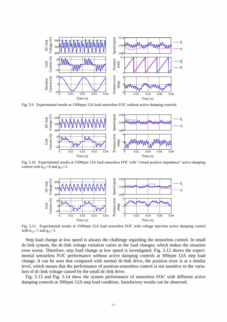
5.2.4 Active Damping with Position Sensorless Control

Since the dc-link voltage is the only dc-link parameter used in the motor control and the dc-link

voltage oscillation increases as the load increases, position-sensorless drive at rated speed and

heavy load should be tested. Fig. 5.9 shows the sensorless FOC performance at 1500rpm 12A load

without active damping control, which is considered to be the worst case as the variation of the dc-

link voltage is maximized. It can be seen that the system can perform well with good speed and

position estimation.

Fig. 5.10 and Fig. 5.11 show the system performance of sensorless FOC with different active

damping controls at 1500rpm 12A load condition. It can be seen that the influence to the perfor-

mance of position and speed estimation is very limited. The injection of the high frequency voltage

and current caused by the active damping control methods brings very little impact to the sensorless

operation performance of the drive system.

- 27 -

0 0.02 0.04 0.06 0.08-6

-5

-4

0

6.4

1490

1500

1510

Po

siti

on

(rad

)

Time (s)

Po

siti

on

err

or

(deg

)

Sp

eed

(rp

m)

0 0.01 0.02 0.03 0.04-20

0

20

-10

0

10

400

500

600

Gri

d

Cu

rren

t (A

)

Time (s)

Mac

hin

e

Cu

rren

t (A

)

DC

-lin

k

Vo

ltag

e (V

)rn

ˆrn

r

ˆr

Fig. 5.9. Experimental results at 1500rpm 12A load sensorless FOC without active damping controls.

1480

1500

1520

0 0.02 0.04 0.06 0.08-6

-5

-4

Po

siti

on

err

or

(deg

)

Time (s)

Sp

eed

(rp

m)

0 0.01 0.02 0.03 0.04

-10

0

10

400

500

600

Gri

d

Cu

rren

t (A

)

Time (s)

DC

-lin

k

Vo

ltag

e (V

)

rn

ˆrn

Fig. 5.10. Experimental results at 1500rpm 12A load sensorless FOC with “virtual positive impedance” active damping

control with krip = 0 and gv0 = 2.

1480

1500

1520

0 0.02 0.04 0.06 0.08-7

-6

-5

0 0.01 0.02 0.03 0.04

-10

0

10

400

500

600

Po

siti

on

err

or

(deg

)

Time (s)

Sp

eed

(rp

m)

Gri

d

Cu

rren

t (A

)

Time (s)

DC

-lin

k

Vo

ltag

e (V

)

rn

ˆrn

Fig. 5.11. Experimental results at 1500rpm 12A load sensorless FOC with voltage injection active damping control

with krip = 1 and gvq = 1.

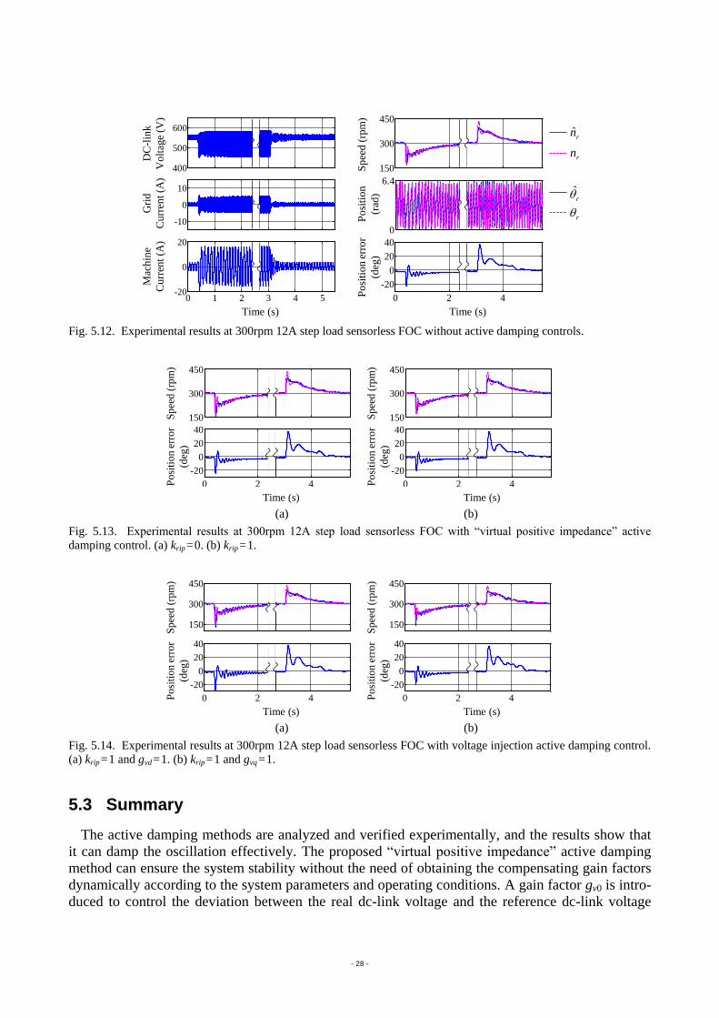
Step load change at low speed is always the challenge regarding the sensorless control. In small

dc-link system, the dc-link voltage variation varies as the load changes, which makes the situation

even worse. Therefore, step load change at low speed is investigated. Fig. 5.12 shows the experi-

mental sensorless FOC performance without active damping controls at 300rpm 12A step load

change. It can be seen that compared with normal dc-link drive, the position error is at a similar

level, which means that the performance of position-sensorless control is not sensitive to the varia-

tion of dc-link voltage caused by the small dc-link drive.

Fig. 5.13 and Fig. 5.14 show the system performance of sensorless FOC with different active

damping controls at 300rpm 12A step load condition. Satisfactory results can be observed.

- 28 -

400

500

600

-10

0

10

0 1 2 3 4 5-20

0

20

Gri

d

Cu

rren

t (A

)

Time (s)

Mac

hin

e

Cu

rren

t (A

)

DC

-lin

k

Vo

ltag

e (V

)150

300

450

0

6.4

0 2 4

-20

0

20

40

Po

siti

on

(rad

)

Time (s)

Po

siti

on

err

or

(deg

)

Sp

eed

(rp

m)

rn

ˆrn

r

ˆr

Fig. 5.12. Experimental results at 300rpm 12A step load sensorless FOC without active damping controls.

0 2 4

-20

0

20

40

150

300

450

Po

siti

on

err

or

(deg

)

Time (s)

Sp

eed

(rp

m)

150

300

450

0 2 4

-20

0

20

40

Po

siti

on

err

or

(deg

)

Time (s)

Sp

eed

(rp

m)

(a) (b)

Fig. 5.13. Experimental results at 300rpm 12A step load sensorless FOC with “virtual positive impedance” active

damping control. (a) krip = 0. (b) krip = 1.

150

300

450

0 2 4

-20

0

20

40

0 2 4

-20

0

20

40

150

300

450

Po

siti

on

err

or

(deg

)

Time (s)

Sp

eed

(rp

m)

Po

siti

on

err

or

(deg

)

Time (s)

Sp

eed

(rp

m)

(a) (b)

Fig. 5.14. Experimental results at 300rpm 12A step load sensorless FOC with voltage injection active damping control.

(a) krip = 1 and gvd = 1. (b) krip = 1 and gvq = 1.

5.3 Summary

The active damping methods are analyzed and verified experimentally, and the results show that

it can damp the oscillation effectively. The proposed “virtual positive impedance” active damping

method can ensure the system stability without the need of obtaining the compensating gain factors

dynamically according to the system parameters and operating conditions. A gain factor gv0 is intro-

duced to control the deviation between the real dc-link voltage and the reference dc-link voltage

- 29 -

used in PWM. The system stability can be ensured when gv0 ≥ 1. The damping effect increases as gv0

increases.

The position-sensorless small dc-link SynRM drive system has been fully examined. The experi-

mental results show that the introduction of the small dc-link and active damping control algorithms

brings very little impact to the performance of the position-sensorless drive. The influence at steady

state conditions is negligible. Small impact can be observed during step load change conditions,

which might be due to the phase/time delay caused by the LPF when obtaining the dc component of

the dc-link voltage. Generally, the system can operate satisfactorily and is robust enough to satisfy

different operation conditions.

- 30 -

6 CONCLUSION

A variable speed SynRM drive system has been studied and tested extensively in this project, in-

cluding position sensorless control, small dc-link active damping control, and their possible interac-

tions.

Position estimation via flux linkage is first investigated, since the focused applications are e.g.

HVAC applications where high dynamic control performance during standstill to low speed opera-

tion range is not required. A commonly used closed-loop flux observer is adopted and it is found

that it cannot always work properly as expected. System oscillation phenomenon can be observed.

Two solutions are proposed and verified. One solution is to enhance the closed-loop observer with a

PR controller, whose cutoff frequency should be adjusted according to the estimated speed. The

other is to damp the oscillation by varying the PI parameters of the speed and current regulators

according to the speed estimation error. The former solution can work very well during the steady-

state conditions. While the latter solution is a more simple and robust solution, especially at the

conditions with sudden speed changes such as step load on or off. Regarding this project, the adap-

tive PI solution is preferred since it can meet the project topic and scope better, i.e. a simple but

robust solution.

Small dc-link drive system, in which the electrolytic dc-link capacitors are replaced with film ca-

pacitors, is obtaining more and more interests from the industrial side, since the film capacitor has

much longer expected service lifetime and also has the potential to achieve a compact design of the

dc-link capacitor bank at high power ratings. However, due to the well-known negative impedance

characteristic of the PWM inverter with constant power load, system instability may occur and ac-

tive damping control may be required.

The active damping methods based on voltage/current injection are summarized. Furthermore, a

virtual positive impedance active damping method is introduced and verified. Compared with the

voltage/current injection solutions, which require on-line calculation of the compensating gain fac-

tors according to the system parameters and operating conditions, this method can ensure the sys-

tem stability without the knowledge of the system parameters and operating conditions. The com-

pensating gain factor introduced in the proposed method is used to control the level of the damping

effect, such as without damping, with damping, twice damping effect, etc. Thus, the compensating

gain factor is a fixed user input, rather than a varying value calculated on-line which may have sta-

bility problem. Therefore, this method is much simple and robust.

Finally, the preferred flux linkage based position estimation method with adaptive PI controllers

is used to cooperate with different active damping methods, so that the whole variable speed

SynRM drive system can be built and tested. It is found that the whole system can perform well.

Based on the above findings, it can be concluded that the whole variable speed SynRM drive sys-

tem can perform well. The solution based on the flux linkage based position estimation method with

adaptive PI controllers and the virtual positive impedance active damping method is preferred and

recommended so far.

6.1 Scientific Contributions

The following contributions can be highlighted:

Closed-loop flux observer analysis is carried out regarding its possible error compensation function.

The limitation of this widely used closed-loop flux observer is found and solutions are pro-

posed and verified.

Virtual positive impedance concept is introduced and analyzed for small dc-link active damping,

- 31 -

which can ensure the system stability without the need of obtaining the compensating gain fac-

tors dynamically according to the system parameters and operating conditions. The damping

effect can be simply controlled by a damping factor.

Small dc-link position sensorless control is carried out. The influence of the active damping control

to the position sensorless drive is studied. Recommendation of the active damping methods is

given from the position sensorless drive point of view.

6.2 Future Work

Though many topics have been addressed and analyzed, there are still some issues that can be im-

proved and require further studies. These issues are summarized as following:

Speed estimation Speed filter is used to provide smooth speed signal for the closed-loop feedback

control. However, phase delay will be caused by the filter and the dynamic performance will

be influenced at e.g. step load change conditions. Therefore, it is of great interest to improve

the speed estimation by proper compensation techniques or predictive control methods.

Sampling delay compensation The sampling delay existing in the DSP system may influence the

performance of the small dc-link active damping methods, especially when the resonant fre-

quency is close to the sampling frequency. Predictive control theory may be adopted to handle

such problem, since the delay is normally known and fixed. Then, it is possible to eliminate

the converter dc choke/inductor in the small dc-link drive system, where the resonant frequen-

cy could be high when connected to stiff grid.

Dc-link voltage ripple prediction The dc-link oscillating voltage, which should be damped by the

control methods, is generally obtained by subtracting the dc-link voltage ripple from the

measured dc-link voltage. However, the dc-link voltage ripple varies for different converter

input and output as well as the system parameters. Therefore, an accurate prediction of the dc-

link voltage ripple will be helpful in finding the correct signal (i.e. the dc-link oscillating volt-

age) that should be damped, so that a better system performance can be finally obtained.

- 32 -

LITERATURE LIST

[1] T. Lipo, “Synchronous Reluctance Machines - A Viable Alternative for AC Drives?,” in Evolu-

tion and Modern Aspects of Synchronous Machines, Zurich, Switzerland, Aug. 1991.

[2] D. Wang, K. Lu, and P. O. Rasmussen, “A general and intuitive approach to understand and

compare the torque production capability of AC machines,” in Proc. ICEMS, Hangzhou, Chi-

na, Oct. 2014, pp. 3136–3142.

[3] “Film technology to replace electrolytic technology,” AVX Co., Fountain Inn, SC, 2005.

[Online]. Available: http://www.avx.com/docs/techinfo/filmtech.pdf

[4] M. Salcone and J. Bond, “Selecting film bus link capacitors for high performance inverter ap-

plications,” in Proc. IEMDC, Miami, FL, May 2009, pp.1692–1699.

[5] P. P. Acarnley, and J.F. Watson, “Review of position-sensorless operation of brushless perma-

nent-magnet machines,” IEEE Trans. Ind. Electron., vol. 53, no. 2, pp. 352–362, Apr. 2006.

[6] K. J. Meessen, P. Thelin, J. Soulard, and E. A. Lomonova, “Inductance Calculations of

Permanent-Magnet Synchronous Machines Including Flux Change and Self- and Cross-

Saturations,” IEEE Trans. on Magnetics, vol. 44, no. 10, pp. 2324–2331 , Oct. 2008.

[7] P. Guglielmi, M. Pastorelli, and A. Vagati, “Impact of Cross-Saturation in Sensorless Control

of Transverse-Laminated Synchronous Reluctance Motors,” IEEE Trans. Ind. Electron., vol.

53, no. 2, pp. 429–439, Apr. 2006.

[8] P. C. Krause, O. Wasynczuk, and S. D. Sudhoff, Analysis of Electric Machinery and Drive

System, 2nd ed., New York: Wiley-IEEE Press, 2002, pp. 481–523.

[9] Z. Wang, K. Lu, and F. Blaabjerg, “A simple startup strategy based on current regulation for

back-EMF-Based sensorless control of PMSM,” IEEE Trans. Power Electron., vol. 27, no. 8,

pp. 3817–3825, Aug. 2012.

[10] I. Boldea, M. C. Paicu, and G. D. Andreescu, “Active flux concept for motion-sensorless uni-

fied AC drives,” IEEE Trans. Power Electron., vol. 23, no. 5, pp. 2612–2618, Sep. 2008.

[11] P. L. Jansen, R. D. Lorenz, and D. W. Novotny, “Observer-based direct field orientation:

Analysis and comparison of alternative methods,” IEEE Trans. Ind. Appl., vol. 30, pp. 945–

953, Jul./Aug. 1994.

[12] S. C. Agarlita, I. Boldea, and F. Blaabjerg, “High-frequency-injection -assisted “active flux”-

based sensorless vector control of reluctance synchronous motors, with experiments from zero

speed,” IEEE Trans. Ind. Appl., vol. 48, no. 6, pp. 1931–1939, Nov./Dec. 2012.

[13] T. Tuovinen, and M. Hinkkanen, “Signal-Injection-Assisted Full-Order Observer With Pa-

rameter Adaptation for Synchronous Reluctance Motor Drives,” IEEE Trans. Ind. Appl., vol.

50, no. 5, pp. 3392–3402, Sep./Oct. 2014.

[14] J. Holtz and J. Quan, “Sensorless vector control of induction motors at very low speed using a

nonlinear inverter model and parameter identification,” IEEE Trans. Ind. Appl., vol. 38, no. 4,

pp. 1087–1095, Jul./Aug. 2002.

[15] A. R. Munoz and T. A. Lipo, “On-line dead-time compensation technique for open-loop PWM-

VSI drives,” IEEE Trans. Power Electron., vol. 14, no. 4, pp. 683–689, Jul. 1999.

[16] H. Zhao, Q. M. J. Wu and A. Kawamura, “An accurate approach of nonlinearity compensation

for VSI inverter output voltage,” IEEE Trans. Power Electron., vol. 19, no. 4, pp.1029–1035,

Jul. 2004.

[17] R. Teodorescu, F. Blaabjerg, M. Liserre, and P. C. Loh, “Proportional- resonant controllers and

filters for grid-connected voltage-source converters,” IEE Proc. Electr. Power Appl., vol.

153, no. 5, pp.750–762, Sep. 2006.

[18] R. Maheshwari, S. Munk-Nielsen, and Kaiyuan Lu, “An active damping technique for small

- 33 -

dc-link capacitor based drive system,” IEEE Trans. on Industrial Informatics, vol. 9, no. 2, pp.

848-858, May 2013.

[19] L. Mathe, H. R. Anderson, R. Lazar, and M. Ciobotaru, “DC-link compensation method for

slim dc-link drives fed by soft grid,” in Proc. ISIE, Bari, Italy, Jul. 2010, pp. 1236–1241.

[20] M. Hinkkanen, L. Harnefors, and J. Luomi, “Control of induction motor drives equipped with

small dc-link capacitance,” in Proc. EPE, Aalborg, Denmark, Sep. 2007, pp. 1–10.

[21] K. Pietilainen, L. Harnefors, A. Petersson, and H.-P. Nee, “DC-link stabilization and voltage

sag ride-through of inverter drives,” IEEE Trans. Ind. Electron., vol. 53, no. 4, pp. 1261–1268,

Aug. 2006.

[22] D. Wang, K. Lu, P. O. Rasmussen, L. Mathe, and Y. Feng, “Analysis of Voltage Modulation

Based Active Damping Techniques for Small DC-Link Drive System,” in Proc. ECCE, Mon-

treal, Canada, Sep. 2015, pp. 2927–2934.

[23] W.-J. Lee and S.-K. Sul, “DC-link voltage stabilization for reduced dc-link capacitor inverter,”

IEEE Trans. Ind. Appl., vol. 50, no. 1, pp. 404–414, Jan. 2014.

[24] S. D. Sudhoff, K. A. Corzine, S. F. Glover, H. J. Hegner, and H. N. Robey, “DC link stabilized

field oriented control of electric propulsion systems,” IEEE Trans. Energy Convers., vol. 13,

no. 1, pp. 27–33, Mar. 1998.

[25] H. Mosskull, J. Galic, and B. Wahlberg, “Stabilization of induction motor drives with poorly

damped input filters,” IEEE Trans. Ind. Electron., vol. 54, no. 5, pp. 2724–2734, Oct. 2007.

[26] P. Magne, D. Marx, B. Nahid-Mobarakeh, and S. Pierfederici, “Large-signal stabilization of a

dc-link supplying a constant power load using a virtual capacitor: Impact on the domain of at-

traction,” IEEE Trans. Ind. Appl., vol. 48, no. 3, pp. 878–887, May/Jun. 2012.

[27] P. Liutanakul, A.-B. Awan, S. Pierfederici, B. Nahid-Mobarakeh, and F. Meibody-Tabar, “Lin-

ear stabilization of a dc bus supplying a constant power load: A general design approach,”

IEEE Trans. Power Electron., vol. 25, no. 2, pp.475–488, Feb. 2010.

[28] Y. A.-R. I. Mohamed, A. A. A. Radwan, and T. K. Lee, “Decoupled reference-voltage-based

active dc-link stabilization for PMSM drives with tight-speed regulation,” IEEE Trans. Ind.

Electron., vol. 59, no. 12, pp.4523–4536, Dec. 2012.

[29] “Harmonics,” Danfoss A/S, Nordborg, Denmark. [Online]. Available:

http://www.danfoss.com/NR/rdonlyres/AF4DDB73-B11C-4886-B1E0-3F76C

1ACDF06/0/inst_po_garmonikam_ENG.pdf

[30] M. Cespedes, T. Beechner, L. Xing, and J. Sun, “Stabilization of constant-power loads by pas-

sive impedance damping,” in Proc. APEC, Palm Springs, CA, Feb. 2010, pp. 2174–2180.

[31] H. Ertl, and J. W. Kolar, “A constant output current three-phase diode bridge rectifier employ-

ing a novel “electronic smoothing inductor”,” IEEE Trans. Ind. Electron., vol. 52, no. 2, pp.

454–461, Apr. 2005.

[32] H. Shin, H.-G. Choi, and J.-I. Ha, “DC-link shunt compensator for three-phase system with

small DC-link capacitor,” in Proc. ICPE-ECCE Asia, Seoul, South Korea, Jun. 2015, pp. 33–

39.

[33] L. Mathe, F. Iov, D. Sera, L. Torok, and R. Teodorescu, “Implementation of PLL and FLL

trackers for signals with high harmonic content and low sampling frequency,” in Proc. OPTIM,

Bran, May 2014, pp. 633–638.