Variance and covariance

n

ii

T

nT

n

a

aaa

a

a

a

1

2

212

1

......

UU

UU

n

ii

n

ii

T

an

an

Variance1

22

1

2

11

11

......

MM

n

ii

T

n

Variancena

a

a

a

1

22

1

)1(...

VVMUV

TT

nnVariance ))((

11

11 2 MUMUVV

Covariance)1(

...;

...

1

2

1

2

1

nba

b

b

b

a

a

a

n

iBiAi

T

Bn

B

B

An

A

A

AB

BA

Sums of squares

General linear models

iancevarCon B

TA

)()(

11

XBXA

The coefficient of correlation

yx

xy

yx

xyr

)cov(

)()'(11

)var(

)()'(11

)var(

)()'(11

)cov(

YY

X

YX

ΜXΜX

ΜXΜX

ΜYΜX

ny

nx

nxy

Y

XX

)()')(()'(

)()'(

YY

YX

ΜYΜYΜXΜX

ΜYΜXR

XX

For a matrix X that contains several variables

holds

The matrix R is a symmetric distance matrix that contains all correlations between the variables

11

11 )()'(1

1

XX

XX

DΣΣR

ΣΜXΜXΣRn

The diagonal matrix SX contains the standard deviations as entries.

X-M is called the central matrix.

We deal with samples

)()'(11

ΜXΜXD

n

MatrixCov

Xn

X

X

X

000

0...00

000

000

2

1

Σ

Linear regression

European bat species and environmental correlates

y = 9.24x0.73

R2 = 0.950.1

1

10

100

1000

10000

100000

0.001 1 1000Body weight [kg]

Bra

in w

eig

ht [

g]

z

Mammals

y = 4.4x0.53

R2 = 0.191

10

100

1000

1 10 100Poplar plantation

Ag

ricu

ltura

l fie

ld

z

Ground beetles at two adjacent sites

There is a hypothesis about dependent and independent variables

The relation is supposed to be linear

We have a hypothesis about the distribution of errors around the hypothesized regression line

There is a hypothesis about dependent and independent variables

The relation is non-linear

We have no data about the distribution of errors around the hypothesized regression line

There is no clear hypothesis about dependent and independent variables

The relation is non-linear

We have no data about the distribution of errors around the hypothesized regression line

y = 1.16x + 4.17

R2 = 0.49

0

20

40

60

80

100

0 10 20 30 40 50# prey species

# p

red

ato

r sp

eci

es

z Assumptions of linear regression

ln(Area)ln(Number

of species)

10.26632 3.2580976.148468 011.33704 3.2188767.696213 0.6931478.519989 2.7080512.24361 2.89037210.3264 2.995732

10.84344 3.17805412.40519 2.89037211.61702 3.4965088.891512 2.1972255.703782 1.6094389.068777 3.0445229.019059 2.83321310.94366 3.5263617.824046 1.0986129.132379 2.89037211.27551 3.17805410.67112 2.6390577.887209 2.63905710.71945 2.3978957.243513 012.73123 2.39789513.20664 3.46573612.78555 3.2188761.871802 1.60943811.7905 3.496508

11.44094 3.33220511.54248 011.16014 2.39789512.6162 3.433987

9.615805 2.56494911.07637 2.7725895.075174 1.79175911.08702 2.6390577.858641 2.89037210.1401 3.178054

6.670766 1.6094385.755742 2.07944210.42552 3.0445220.667829 08.265136 2.1972259.557046 2.07944212.68838 2.39789512.65321 3.17805411.42796 3.17805412.37772 3.40119715.25979 3.4011974.110874 010.07799 2.99573211.53468 3.36729610.14353 3.09104210.80058 3.3322059.917045 3.29583713.13427 3.46573611.03568 013.01692 2.89037210.62825 3.36729610.63432 2.83321310.07593 3.25809713.31114 3.258097-0.82098 0

N=62

)ln()ln( 10 AaaS

1

02

1

2

1

102

1

1

......

1

1

...

1

...

1

1

... a

a

x

x

x

x

x

x

aa

y

y

y

nnn

Y

XAY

Matrix approach to linear regression

YXXXA

AIAXAXXXYXXX

XAXYX

''

''''

''

1

11

X is not a square matrix, hence X-1 doesn’t exist.

The species – area relationship of European bats

ln(Number of

species)Constant ln(Area) X'

3.258097 1 10.26632 1 1 1 1 1 1 1 1 1 1 1 1 10 1 6.148468 10.26632 6.148468 11.33704 7.696213 8.519989 12.24361 10.3264 10.84344 12.40519 11.61702 8.891512 5.703782 9.068777

3.218876 1 11.337040.693147 1 7.696213 X'X2.70805 1 8.519989 62 607.1316

2.890372 1 12.24361 607.1316 6518.161

2.995732 1 10.3264 (X'X)-1

3.178054 1 10.84344 0.183521 -0.017092.890372 1 12.40519 -0.01709 0.0017463.496508 1 11.617022.197225 1 8.8915121.609438 1 5.703782 X'Y3.044522 1 9.068777 154.29372.833213 1 9.019059 1647.9083.526361 1 10.943661.098612 1 7.824046

2.890372 1 9.132379 (X'X)-1(X'Y)3.178054 1 11.27551 a0 0.1468082.639057 1 10.67112 a1 0.2391442.639057 1 7.8872092.397895 1 10.71945

0 1 7.2435132.397895 1 12.731233.465736 1 13.206643.218876 1 12.785551.609438 1 1.8718023.496508 1 11.7905

y = 0.2391x + 0.1468R² = 0.4614

-0.5

0

0.5

1

1.5

2

2.5

3

3.5

4

-5 0 5 10 15 20

ln(#

spe

cies

)

ln (Area)

What about the part of variance explained by our model?

11 )()'(11

XX ΣΜXΜXΣRn

24.024.015.0 16.1

15.0ln24.0ln

AAeS

AS

1.16: Average number of species per unit area (species density)

0.24: spatial species turnover

11 )()'(11

XX ΣΜXΜXΣRn

X-M (X-M)'

0.769488 0.473878 0.769488 -2.48861 0.730267 -1.79546 0.219442 0.401763-2.48861 -3.64398 0.473878 -3.64398 1.54459 -2.09623 -1.27246 2.4511640.730267 1.54459-1.79546 -2.096230.219442 -1.27246 (X-M)'(X-M) (X-M)'(X-M) / (n-1)0.401763 2.451164 71.0087 136.9954 1.164077 2.2458260.507124 0.533954 136.9954 572.8582 2.245826 9.3911190.689445 1.0509910.401763 2.612741 Sx1.007899 1.824579 1.078924 0-0.29138 -0.90093 0 3.064493-0.87917 -4.08866

0.555914 -0.72367 Sx-1

0.344605 -0.77339 0.926849 01.037752 1.151213 0 0.326318

-1.39 -1.9684

0.401763 -0.66007 Sx-1 (X-M)'(X-M) / (n-1)0.689445 1.48306 1.078924 2.0815420.150449 0.878671 0.732854 3.0644930.150449 -1.90524-0.09071 0.927004-2.48861 -2.54893 Sx-1 (X-M)'(X-M) / (n-1) Sx-1-0.09071 2.938785 1 0.6792450.977127 3.414195 0.679245 10.730267 2.993105-0.87917 -7.92064

1.007899 1.998051 Sx-1 (X-M)'(X-M) / (n-1) Sx-1)2

0.843596 1.64849 1 0.461374-2.48861 1.750039 0.461374 1-0.09071 1.3676980.945379 2.8237520.076341 -0.17664

y = 0.2391x + 0.1468R² = 0.4614

-0.5

0

0.5

1

1.5

2

2.5

3

3.5

4

-5 0 5 10 15 20

ln(#

spe

cies

)

ln (Area)

n

iiMY YY

n 1

22; )(

11y = 0.2391x + 0.1468

R² = 0.4614

-0.5

0

0.5

1

1.5

2

2.5

3

3.5

4

-5 0 5 10 15 20

ln(#

spe

cies

)

ln (Area)

How to interpret the coefficient of determination

n

ii

n

ii

n

ii

n

iii

YY

YXY

YYn

XYYn

variance Totalvariance Residual

R

1

2

1

2

1

2

1

2

2

)(

))((

)(11

))((11

11

dfR

RF 2

2

1Statistical testing

is done by an F or a t-test.

2);(

2)(;

2; MXYXYYMY

n

iiiXYY XYY

n 1

22)(; ))((

11

n

iiMXY YXY

n 1

22);( ))((

11

dfR

Rt

Ft

21

Total variance

Rest (unexplained) variance

Residual (explained) variance

LaNaTaAaaS T 403210 )ln()ln(

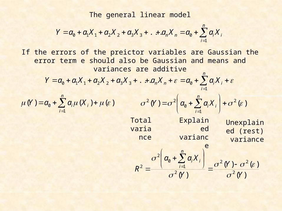
The general linear model

n

iiinn XaaXaXaXaXaaY

103322110 ...

A model that assumes that a dependent variable Y can be expressed by a linear combination of predictor variables X is called a linear model.

XAY

nnmm

n

n

m y

y

a

xx

xx

xx

y

y

y

...

...1

.........1

...1

...1

...1

0

,1,

,21,2

,11,1

2

1

YXXXA

AIAXAXXXYXXX

XAXYX

''

''''

''

1

11

ΕXAY

nnnmm

n

n

m y

y

a

xx

xx

xx

y

y

y

......

...1

.........1

...1

...1

...1

0

1

0

,1,

,21,2

,11,1

2

1

The vector E contains the error terms of each regression. Aim is to minimize E.

The general linear model

n

iiinn XaaXaXaXaXaaY

103322110 ...

n

iiinn XaaXaXaXaXaaY

103322110 ...

If the errors of the preictor variables are Gaussian the error term e should also be Gaussian and means and variances are additive

)()()(1

0

n

iii XaaY )()( 2

10

22

n

iii XaaY

Total variance

Explained variance

Unexplained (rest)

variance

)()()(

)( 2

22

21

02

2

YY

Y

Xaa

R

n

iii

LaNaAaaS T 40310 )ln()ln(

1. Model formulation2. Estimation of model parameters

3. Estimation of statistical significance

YXXXA

XAY

'' 1

Y

Country/Islandln(Number

of species)

Constant ln(Area)Days below zero

Latitude of capitals (decimal degrees)

Albania 3.258097 1 10.26632 34 41.33Andorra 0 1 6.148468 60 42.5Austria 3.218876 1 11.33704 92 48.12Azores 0.693147 1 7.696213 1 37.73Baleary Islands 2.70805 1 8.519989 18 39.55Belarus 2.890372 1 12.24361 144 53.87Belgium 2.995732 1 10.3264 50 50.9Bosnia and Herzegovina 3.178054 1 10.84344 114 43.82British islands 2.890372 1 12.40519 64 51.15Bulgaria 3.496508 1 11.61702 102 42.65Canary Islands 2.197225 1 8.891512 1 27.93Channel Is. 1.609438 1 5.703782 12 49.22Corsica 3.044522 1 9.068777 11 41.92Crete 2.833213 1 9.019059 1 35.33Croatia 3.526361 1 10.94366 114 45.82Cyclades Is. 1.098612 1 7.824046 1 37.1Cyprus 2.890372 1 9.132379 2 35.15Czech Republic 3.178054 1 11.27551 119 50.1Denmark 2.639057 1 10.67112 85 55.63Dodecanese Is. 2.639057 1 7.887209 2 36.4Estonia 2.397895 1 10.71945 143 59.35Faroe Is. 0 1 7.243513 35 62Finland 2.397895 1 12.73123 169 60.32France 3.465736 1 13.20664 50 48.73Germany 3.218876 1 12.78555 97 52.38Gibraltar 1.609438 1 1.871802 0 36.1Greece 3.496508 1 11.7905 2 37.9Hungary 3.332205 1 11.44094 100 47.43Iceland 0 1 11.54248 133 64.13

X

Multiple regression

X'

1 1 1 1 1 1 1 110.26632 6.148468 11.33704 7.696213 8.519989 12.24361 10.3264 10.84344

34 60 92 1 18 144 50 11441.33 42.5 48.12 37.73 39.55 53.87 50.9 43.82

X'X62 607.1316 4328 2906.4

607.1316 6518.161 48545.59 29086.574328 48545.59 534136 228951.7

2906.4 29086.57 228951.7 141148.1

(X'X)-1

1.019166 -0.02275 0.00261 -0.02053-0.02275 0.002458 -7.5E-05 8.3E-050.00261 -7.5E-05 1.3E-05 -5.9E-05

-0.02053 8.3E-05 -5.9E-05 0.000509

(X'X)-1X'0.025783 0.163309 0.013407 0.07203 0.060295 0.010457 -0.13031 0.1703470.003376 -0.00859 0.002243 -0.00078 0.00013 0.001069 0.003124 -0.00097-0.00017 0.000405 9.87E-05 -0.00019 -0.00014 0.000364 -0.00054 0.000676-0.00066 -0.00195 -0.00056 -0.00074 -0.00076 -0.00064 0.003269 -0.00409

(X'X)-1X'Y X'Y (X'X)-1(X'Y)a0 2.679757 154.2937 2.679757a1 0.290121 1647.908 0.290121a2 0.002155 11289.32 0.002155a3 -0.06789 7137.716 -0.06789

Multiple R and R2

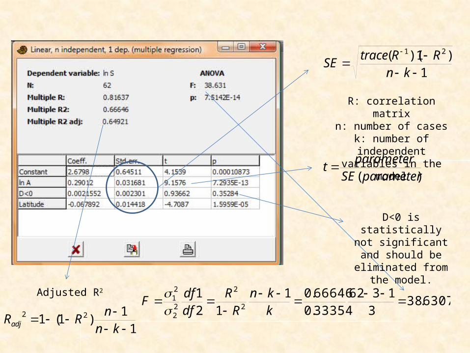
Adjusted R2

6307.383

136233354.066646.01

121

2

2

22

21

kkn

RR

dfdf

F

R: correlation matrixn: number of cases

k: number of independent variables in the model

)( parameterSEparameter

t

11

)1(1 22

kn

nRRadj

D<0 is statistically not significant and should

be eliminated from the model.

1)1)(( 21

knRRtrace

SE

Y

Country/Islandln(Number

of species)

Constant ln(Area)Days below zero

Latitude of capitals (decimal degrees)

Latitude2 X'

Albania 3.258097 1 10.26632 34 41.33 1708.169 1 1 1 1 1 1 1 1Andorra 0 1 6.148468 60 42.5 1806.25 10.26632 6.148468 11.33704 7.696213 8.519989 12.24361 10.3264 10.84344Austria 3.218876 1 11.33704 92 48.12 2315.534 34 60 92 1 18 144 50 114Azores 0.693147 1 7.696213 1 37.73 1423.553 41.33 42.5 48.12 37.73 39.55 53.87 50.9 43.82Baleary Islands 2.70805 1 8.519989 18 39.55 1564.203 1708.169 1806.25 2315.534 1423.553 1564.203 2901.977 2590.81 1920.192Belarus 2.890372 1 12.24361 144 53.87 2901.977Belgium 2.995732 1 10.3264 50 50.9 2590.81 X'XBosnia and Herzegovina 3.178054 1 10.84344 114 43.82 1920.192 62 607.1316 4328 2906.4 141148.1British islands 2.890372 1 12.40519 64 51.15 2616.323 607.1316 6518.161 48545.59 29086.57 1441737Bulgaria 3.496508 1 11.61702 102 42.65 1819.023 4328 48545.59 534136 228951.7 12488619Canary Islands 2.197225 1 8.891512 1 27.93 780.0849 2906.4 29086.57 228951.7 141148.1 7106497Channel Is. 1.609438 1 5.703782 12 49.22 2422.608 141148.1 1441737 12488619 7106497 3.71E+08Corsica 3.044522 1 9.068777 11 41.92 1757.286Crete 2.833213 1 9.019059 1 35.33 1248.209 (X'X)-1

Croatia 3.526361 1 10.94366 114 45.82 2099.472 6.45421 0.000497 0.001087 -0.25606 0.002409Cyclades Is. 1.098612 1 7.824046 1 37.1 1376.41 0.000497 0.002557 -8.1E-05 -0.00092 1.03E-05Cyprus 2.890372 1 9.132379 2 35.15 1235.523 0.001087 -8.1E-05 1.34E-05 6.63E-06 -6.8E-07Czech Republic 3.178054 1 11.27551 119 50.1 2510.01 -0.25606 -0.00092 6.63E-06 0.010716 -0.0001Denmark 2.639057 1 10.67112 85 55.63 3094.697 0.002409 1.03E-05 -6.8E-07 -0.0001 1.07E-06Dodecanese Is. 2.639057 1 7.887209 2 36.4 1324.96Estonia 2.397895 1 10.71945 143 59.35 3522.423 (X'X)-1X'Faroe Is. 0 1 7.243513 35 62 3844 0.028519 -0.00857 -0.18332 0.227512 0.119213 -0.18587 -0.27812 -0.01106Finland 2.397895 1 12.73123 169 60.32 3638.502 0.003388 -0.00932 0.001402 -0.00011 0.000382 0.000229 0.002492 -0.00174France 3.465736 1 13.20664 50 48.73 2374.613 -0.00017 0.000453 0.000154 -0.00024 -0.00016 0.000419 -0.00049 0.000727Germany 3.218876 1 12.78555 97 52.38 2743.664 -0.00078 0.0055 0.007968 -0.00748 -0.00331 0.007864 0.009674 0.003767Gibraltar 1.609438 1 1.871802 0 36.1 1303.21 1.21E-06 -7.6E-05 -8.7E-05 6.89E-05 2.61E-05 -8.7E-05 -6.6E-05 -8E-05Greece 3.496508 1 11.7905 2 37.9 1436.41Hungary 3.332205 1 11.44094 100 47.43 2249.605 (X'X)-1X'YIceland 0 1 11.54248 133 64.13 4112.657 a0 -3.40816Ireland 2.397895 1 11.16014 23 53.43 2854.765 a1 0.264082Italy 3.433987 1 12.6162 18 41.8 1747.24 a2 0.003862Kaliningrad Region 2.564949 1 9.615805 110 52.7 2777.29 a3 0.195932Latvia 2.772589 1 11.07637 124 56.96 3244.442 a4 -0.0027

X

A mixed model2

430210 lnln LaLaDaAaaS T

20 0027.0196.0004.0ln26.041.3ln LLDAS T

The final model

Is this model realistic?

Very low species density (log-scale!)

Realistic increase of species richness with

area

Increase of species richness with winter

length

Increase of species richness at higher

latitudes

A peak of species richness at

intermediate latitudes

The model makes realistic predictions.

Problem might arise from the intercorrelation between the predictor variables

(multicollinearity).

We solve the problem by a step-wise approach eliminating the variables that are either not significant or give unreasonable parameter

values

The variance explanation of this final model is higher than that of the previous one.

y = 0.6966x + 0.7481R² = 0.6973

-1-0.5

00.5

11.5

22.5

33.5

44.5

0 1 2 3 4

ln(#

spe

cies

pre

dict

ed)

ln (# species observed)

......... 33221

3223

2222221

3113

211211110 XaXaXaXaXbXaXaXaXaaY nnn

Multiple regression solves systems of intrinsically linear algebraic equations

YXXXA '' 1

• The matrix X’X must not be singular. It est, the variables have to be independent. Otherwise we speak of multicollinearity. Collinearity of r<0.7 are in most cases tolerable.

• Multiple regression to be safely applied needs at least 10 times the number of cases than variables in the model.

• Statistical inference assumes that errors have a normal distribution around the mean.• The model assumes linear (or algebraic) dependencies. Check first for non-linearities. • Check the distribution of residuals Yexp-Yobs. This distribution should be random.• Check the parameters whether they have realistic values.

y = 0.6966x + 0.7481R² = 0.6973

-1-0.5

00.5

11.5

22.5

33.5

44.5

0 1 2 3 4

ln(#

spe

cies

pre

dict

ed)

ln (# species observed)

Multiple regression is a hypothesis testing and not a hypothesis generating

technique!!

Polynomial regression General additive model

Standardized coefficients of correlation

x

ZZ-tranformed distributions have a mean of 0 an a standard deviation of 1.

YXXX ZZZZB '' 1n

i i n ni 1 i i

X Yi 1 i 1X Y X Y

(X X)(Y Y)(X X) (Y Y)1 1 1

r Z Zn 1 s s n 1 s s n 1

nnn

n

iiiiini

nniii

rr

rr

nR

ZxZxZxZx

ZxZxZxZx

......

............

............

.......

'11

......

............

............

......

'

1

111

1

111

ZZZZ

XYxx RRB 1

In the case of bivariate regression Y = aX+b, Rxx = 1.Hence B=RXY.

Hence the use of Z-transformed values results in standardized correlations coefficients, termed b-values

ZZR '11

n

BRR XXXY