variants of dynamic mode decomposition: boundary conditions
TRANSCRIPT

Variants of dynamic mode decomposition: boundary conditions,
Koopman, and Fourier analyses∗
Kevin K. Chen,†‡ Jonathan H. Tu,† and Clarence W. Rowley†
Oct 24, 2011
Abstract
Dynamic mode decomposition (DMD) is an Arnoldi-like method based on the Koopmanoperator that analyzes empirical data, typically generated by nonlinear dynamics, and computeseigenvalues and eigenmodes of an approximate linear model. Without explicit knowledge of thedynamical operator, it extracts frequencies, growth rates, and spatial structures for each mode.We show that expansion in DMD modes is unique under certain conditions. When constructingmode-based reduced-order models of partial differential equations, subtracting a mean from thedata set is typically necessary to satisfy boundary conditions. Subtracting the mean of the dataexactly reduces DMD to the temporal discrete Fourier transform (DFT); this is restrictive andgenerally undesirable. On the other hand, subtracting an equilibrium point generally preservesthe DMD spectrum and modes. Next, we introduce an “optimized” DMD that computes anarbitrary number of dynamical modes from a data set. Compared to DMD, optimized DMD issuperior at calculating physically relevant frequencies, and is less numerically sensitive. We testthese decomposition methods on data from a two-dimensional cylinder fluid flow at a Reynoldsnumber of 60. Time-varying modes computed from the DMD variants yield low projectionerrors.
∗Submitted to the Journal of Nonlinear Science†Department of Mechanical & Aerospace Engineering, Princeton University, Princeton, NJ 08544‡Email address for correspondence: [email protected]
Variants of dynamic mode decomposition

1 Introduction
Data-based modal decomposition is frequently employed to investigate complex dynamical systems.When dynamical operators are too sophisticated to analyze directly—because of nonlinearity andhigh dimensionality, for instance—data-based techniques are often more practical. Such methodsnumerically analyze empirical data produced by experiments or simulations, yielding modes con-taining dynamically significant structures. In fluid flow control, for example, decompositions ofan evolving flow field may identify coherent structures such as vortices and eddies that are fun-damental to the underlying flow physics (Holmes et al. 1996). A subset of the computed modescan then form the basis of a reduced-order model—that is, a low-dimensional approximation of theoriginal dynamical system—using Galerkin projection. This is often critical in applications such ascontroller or observer design in a control system, where matrix operations on a high-dimensionaldynamical system could be computationally intractable.
One common decomposition technique, proper orthogonal decomposition (POD, otherwiseknown as principal component analysis or Karhunen-Loeve decomposition), generates orthogonalmodes that optimally capture the vector energy of a given data set (Holmes et al. 1996). Thismethod, while popular, suffers from a number of known issues. For instance, reduced-order modelsgenerated by POD may be inaccurate, because the principal directions in a set of data may notnecessarily correspond with the dynamically important ones. As a result, the selection of PODmodes to retain in a reduced-order model is nontrivial and potentially difficult (Ilak and Rowley2008). Improved methods are available, such as balanced truncation (Moore 1981) or balancedPOD (an approximation of balanced truncation for high-dimensional systems; Rowley 2005), butboth of these methods are applicable only to linear systems.
Dynamic mode decomposition (DMD) is a relatively recent development in the field ofmodal decomposition (Rowley et al. 2009; Schmid 2010). Dynamic mode decomposition approx-imates the modes of the Koopman operator, which is a linear, infinite-dimensional operator thatrepresents nonlinear, finite-dimensional dynamics without linearization (Mezic and Banaszuk 2004;Mezic 2005), and is the adjoint of the Perron-Frobenius operator. The method can be viewed ascomputing, from empirical data, eigenvalues and eigenvectors of a linear model that approximatesthe underlying dynamics, even if those dynamics are nonlinear. Unlike POD and balanced POD,this decomposition yields growth rates and frequencies associated with each mode, which can befound from the magnitude and phase of each corresponding eigenvalue. If the data are generated bya linear dynamical operator, then the decomposition recovers the leading eigenvalues and eigenvec-tors of that operator; if the data are periodic, then the decomposition is equivalent to a temporaldiscrete Fourier transform (DFT) (Rowley et al. 2009). Applications of DMD to experimental andnumerical data can be found in Rowley et al. (2009), Schmid (2010, 2011), and Schmid et al. (2011).
In this paper, we present some new properties and some modifications of DMD, highlightingthe relationship with traditional Fourier analysis. Section 2 briefly reviews the Koopman operator,DMD, and two algorithms for computing DMD. In Section 3, we prove the uniqueness of thedecomposition under specific conditions. Section 4 discusses applications to reduced-order modelsof partial differential equations, and in particular compares methods to ensure that models basedon DMD satisfy boundary conditions correctly. We explore the subtraction of either the data meanor an equilibrium point (in fluid mechanics, this is commonly known as “subtracting a base flow”),and examine the consequences of each. In Section 5, we present advances toward an alternate,“optimized” DMD formulation, which tailors the decomposition to the user-specified number ofmodes, and is more accurate than truncated DMD models. We provide examples in Section 6 byconsidering numerically generated data of a cylinder fluid flow, evolving via the nonlinear Navier-Stokes equations from an unstable equilibrium to a limit cycle.
2
2 The Koopman operator and dynamic mode decomposition
In this section, we briefly review the results of Rowley et al. (2009). The Koopman operator U isdefined for a dynamical system
ξk+1 = f (ξk) (1)
evolving on a finite-dimensional manifold M . (The dynamics need not be discrete in time, but weretain this form since we presume that the data to be analyzed are such.) It acts on scalar functionsg : M → R or C according to
Ug (ξ) , g (f (ξ)) . (2)
Although the underlying dynamics are nonlinear and finite-dimensional, the Koopman operator isa linear infinite-dimensional operator; the linearity property is a result of the definition in (2), notlinearization. Given the eigendecomposition
Uφj (ξ) = λjφj (ξ) , j = 1, 2, . . . (3)
of U , we can generally express vector-valued “observables” g : M → Rn or Cn of our choice interms of the Koopman eigenfunctions φj by
g (ξ) =∞∑j=1
φj (ξ) vj , (4)
where vj∞j=1 is a set of vector coefficients called Koopman modes. (Here, we assume that eachcomponent of g lies within the span of the eigenfunctions.) Using (3) and the definition in (2), wecan explicitly write
g (ξk) =∞∑j=1
λkjφj (ξ0) vj . (5)
The Koopman eigenvalues λj∞j=1 therefore dictate the growth rate and frequency of each mode.1
For simplicity, we will hereafter incorporate the constant φj (ξ0) into vj .It is straightforward to show that, if the dynamics (1) are linear, with f(ξ) = Aξ, then the
eigenvalues λj of A are also eigenvalues of the Koopman operator. Furthermore, if the observableis g(ξ) = ξ, then the Koopman modes vj are the corresponding eigenvectors of A (Rowley et al.2009).
The practical idea behind the Koopman analysis is to collect a set of data ξk, identifyan observable g of interest from the data, and express the observable in terms of Koopman modesand eigenvalues. For example, an experimenter may wish to collect fluid flow data from a windtunnel experiment, measuring three-component velocity fields in a spatial region of interest, anddecompose the fields into eigenvalues and modes containing spatial structures.
The DMD algorithm approximates Koopman modes and eigenvalues from a finite set ofdata. The algorithm itself, described in Rowley et al. (2009) and Schmid (2010), is a variant ofa standard Arnoldi method, and we summarize it here. Suppose that the vector observable isexpressed by g (ξk) = xk. The algorithm operates on the real or complex data set xkmk=0 and
1In ergodic theory, the map f is assumed to be measure preserving, making the Koopman operator unitary(Petersen 1983). Here, we make no such assumption, allowing for the analysis of dynamics not lying on an attractor.As such, the growth rates given by |λj | may differ from unity.
3

identifies complex Ritz values λjmj=1 and complex Ritz vectors vjmj=1 such that
xk =m∑j=1
λkjvj , k = 0, . . . ,m− 1 (6a)
xm =m∑j=1
λmj vj + r, r ⊥ span (x0, . . . ,xm−1) , (6b)
provided that λjmj=1 are distinct. This algorithm approximates the data—potentially generatedby a nonlinear process—as the trajectory of a linear system. The first m data vectors are exactlyrepresented by Ritz values and vectors. Projecting the final data vector, however, results in aresidual r that is orthogonal to all previous data vectors, and hence to all Ritz vectors as well.
The computation of DMD modes proceeds as follows. Let K ,[x0 · · · xm−1
]be a data
matrix. Let c =[c0 · · · cm−1
]Tbe a vector of coefficients that best constructs (in a least squares
sense) the final data vector xm as a linear combination of all previous data vectors. That is,
xm = Kc + r, r ⊥ span (x0, . . . ,xm−1) . (7)
One solution for c is given byc = K+xm, (8)
where (·)+ indicates the Moore-Penrose pseudoinverse. The solution for (7) is unique if and only ifK has linearly independent columns; in this case, we can use the pseudoinverse expansion K+ =(K∗K)−1 K∗. Now construct the companion matrix
C ,
0 0 · · · 0 c0
1 0 · · · 0 c1
0 1 0 c2...
. . ....
0 0 1 cm−1
. (9)
One possible diagonalization of this matrix is
C = T−1ΛT, (10)
where Λ is a diagonal matrix with λ1, . . . , λm on the diagonal, T is the Vandermonde matrix definedby Tij , λj−1
i , and λjmj=1 are distinct. The matrix Λ yields the Ritz values. Finally, the Ritz
vectors are given by V ,[v1 · · · vm
], where
V = KT−1. (11)
To understand how this algorithm yields the decomposition in (6), consider that an index-shifted data matrix K∗ ,
[x1 · · · xm
]can be written
K∗ = KC + reT (12a)
= KT−1ΛT + reT, (12b)
if e ,[0 · · · 0 1
]T. Finally, using (11), we obtain
K = VT (13a)
K∗ = VΛT + reT, (13b)
4
which together are equivalent to (6).The algorithm above is analytically correct, but may be ill-conditioned in practice. This
may especially be the case when using noisy experimental data. Schmid (2010) recommends thefollowing alternate algorithm, which is exact when K is full-rank. Let K = UΣW∗ be the economy-sized singular value decomposition (SVD) of K. Solve the diagonalization problem
U∗K∗WΣ−1 = YΛY−1 (14)
and set V = UY; Λ is as above. Finally, scale each column of V by the appropriate complex scalarso that (6a) is satisfied.
For data sets with dim (xk) m, we recommend a method of snapshots approach. In fluidmechanics, for instance, K may (very roughly) have a row dimension O
(105)
to O(1010
)and a
column dimension O(101)
to O(103). In this case, K∗K is much smaller than K. The method
of snapshots can be carried out with lower memory requirements, and may be faster to compute.Evaluate the matrix K∗K, and perform the diagonalization
K∗K = WΣ2W∗. (15)
The diagonal matrix Σ with positive entries and the unitary matrix W are as above. Completethe algorithm of Schmid above, starting at (14), with the substitution U = KWΣ−1.
A key advantage of the SVD and method of snapshots approaches comes to light when K isrank-deficient or nearly so. In this case, the parts of U, Σ, and W corresponding to small singularvalues can be truncated to approximate (6) with a smaller number of modes (Schmid 2010).
3 Uniqueness of dynamic mode decomposition
Rowley et al. (2009) proved by construction that for a set of real or complex data xkmk=0, thereexist complex λjmj=1 and vjmj=1 such that (6) is satisfied, provided that λjmj=1 are distinct.Here, we extend this result by showing that the decomposition is unique.
Theorem 1. The choice of λjmj=1 and vjmj=1 in (6) is unique up to a reordering in j, if and
only if xkm−1k=0 are linearly independent and λjmj=1 are distinct.
Proof. We begin with the backward proof. Since λj are distinct, the Vandermonde matrix T isfull-rank. Recall that (6a) is equivalent to K = VT, and that we assume K is full-rank. It followsthat V is full-rank, and that xkm−1
k=0 and vjmj=1 must each be linearly independent bases of thesame space. Equations (6b, 7) therefore imply that xm can be decomposed into two additive parts,
m∑j=1
λmj vj = Kc ∈ span (x0, . . . ,xm−1) (16)
and r ⊥ span (x0, . . . ,xm−1).Let us rewrite (16) as
V
λm1...λmm
= Kc (17a)
= VTc. (17b)
5
Given that the columns of V are linearly independent, this then reduces toλm1...λmm
= Tc, (18)
from which we extract m scalar equations
λm1 = c0 + c1λ1 + c2λ21 + · · ·+ cm−1λ
m−11
...
λmm = c0 + c1λm + c2λ2m + · · ·+ cm−1λ
m−1m .
(19)
Therefore, the m distinct values of λj are precisely the m roots of the polynomial
p (λ; c) , λm −m−1∑k=0
ckλk. (20)
(By extension, we may also write p (λ; c) =∏m
j=1 (λ− λj); this will be used later.) Note from (8)
that for linearly independent xkm−1k=0 , ckm−1
k=0 exists and is unique. Thus, the m roots λjmj=1
of p (λ; c) must be unique as well, up to a reordering in j. Finally, the vectors vjmj=1 must beunique, as a result of (11).
Next, we show by contradiction that if xkm−1k=0 are linearly dependent or λjmj=1 are not
distinct, then the choice of λjmj=1 and vjmj=1 is not unique, even beyond a reordering in j. Thelatter condition is straightforward to prove—suppose that λq = λr for some q 6= r. Then for anyarbitrary v∗ ∈ Cn, vq may be replaced with vq + v∗, and vr with vr − v∗, and (6) will still hold.
Suppose now that xkm−1k=0 are linearly dependent, so rank (K) < m. We maintain the con-
dition that the λj be distinct; otherwise we refer back to the statement just proven. Thus, the Van-dermonde matrix T is full-rank, so rank (V) = rank (K) < m; furthermore, span (x0, . . . ,xm−1) =span (v1, . . . ,vm).
The remainder of this proof follows similarly to the backward proof. One difference, how-ever, is that c must be non-unique because K does not have full column rank. To be precise,dim (Ker (K)) > 0; if some c satisfies (7), then c + c∗ does as well, for any c∗ ∈ Ker (K). Inaddition, (18, 19) are now sufficient but not necessary for (17). In other words, the m solutions tothe polynomial equation p (λ; c) = 0, along with V = KT−1, are sufficient for satisfying (6).
Since c is not unique, there must exist different coefficient sets ckm−1k=0 and dkm−1
k=0 suchthat
λm −m−1∑k=0
ckλk =
m∏j=1
(λ− λj) = 0 (21a)
µm −m−1∑k=0
dkµk =
m∏j=1
(µ− µj) = 0 (21b)
produce roots λjmj=1 and µjmj=1 each satisfying (6). If λjmj=1 and µjmj=1 are identical, then
according to the above relations, ckm−1k=0 and dkm−1
k=0 must also be identical. Since the coefficientsets are different, however, there must exist distinct sets λjmj=1 and µjmj=1 satisfying (6).
Remark. The polynomial p (λ; c), defined in (20), is precisely the characteristic polynomial of thecompanion matrix in (9) used to construct the DMD. Thus, as in (10), the scalars λjmj=1 are theeigenvalues of C.
6

4 Boundary condition handling
4.1 Overview
An important application of modal decompositions, such as POD or DMD, is to obtain low-dimensional approximations of partial differential equations. When used in this setting, the gov-erning dynamics (1) become infinite dimensional, although in practice, one often uses approximatenumerical solutions (e.g., using finite-difference or spectral methods), and can treat these as sys-tems with large, but finite, dimension. Modal decompositions such as POD and DMD may thenbe used to obtain further approximations of surprisingly low dimension, by expanding the solutionin terms of a linear combination of modes (Holmes et al. 1996).
Of course, partial differential equations differ fundamentally from initial value ordinarydifferential equations and maps in that they require boundary conditions. Subtleties of imposingboundary conditions on such low-dimensional models are frequently overlooked, for instance aspointed out in Noack et al. (2005), but in many cases, the situation is straightforward. For instance,in a fluid flow, often the boundaries of the domain are at a physical boundary (a wall), where velocityis zero, and a simple Dirichlet boundary condition is appropriate. Other cases such as inflow oroutflow conditions can be more difficult, but in practice, often a Dirichlet or Neumann boundarycondition suffices for constructing low-dimensional models. When POD or DMD modes are usedin these situations, careful attention must be given to ensure that the boundary conditions aresatisfied, at least approximately, by the low-dimensional models.
In this section, we consider the case where the dynamics (1) represent an approximationof a partial differential equation, discretized in both time and space, and the observable x = g(ξ)consists of the dependent variables in some spatial region Ω. This is a common situation for fluidflows, since flow information is typically known only in a limited region of space, whether data isobtained from experiments or from numerical simulations. We consider boundary conditions of theform
B (x) = γ, (22)
whereB maps the observed variables x to certain values on the boundary ∂Ω. Suppose the boundarycondition also satisfies the linearity condition
B (α1x1 + α2x2) = α1B (x1) + α2B (x2) . (23)
Given a set of modes vjmj=1, one may construct a low-dimensional approximation of the solutionby expanding x as a linear combination of modes. Using x(k) to denote xk from the previoussection, we have the expansion
x(k) = xb +
m∑j=1
aj(k)vj , (24)
where the constant offset xb is commonly referred to as a “base flow” in the context of fluids. It isthen convenient to require that the base flow itself satisfy the boundary conditions:
B(xb) = γ. (25)
Equations (22–25) imply that for a set x(k)mk=0 of observations each satisfying (22),
B(x(k)− xb) = 0, k = 0, . . . ,m. (26)
That is, if each solution x(k) satisfies the boundary conditions, then the subtraction of the baseflow from each solution attains homogeneous boundary conditions. As a result, modes decomposedfrom the base-flow-subtracted solutions also acquire homogeneous boundary conditions.
7

Therefore, given a set of modes vjmj=1 constructed from base-flow-subtracted data, thenas long as the base flow xb satisfies (25), the expansion (24) will also satisfy the boundary condi-tions (22), for any choice of aj(k). When employing DMD modes computed without first subtractinga base flow, it is generally not possible to satisfy boundary conditions. The modes will typicallyhave nonzero boundary conditions, and any nonzero values along those mode boundaries will bescaled by aj(k).
In the application of POD, it is common to use the mean of a data set as the base flow (e.g.,Noack et al. 2003). We show in the following sections, however, that the use of the data mean asthe base flow exactly reduces DMD to the temporal DFT, and that this is typically undesirable. Onthe other hand, using an equilibrium point as the base flow leads to better-behaved decompositions.
4.2 Mean subtraction
The data mean we describe here is defined by
x ,1
m+ 1
m∑k=0
xk, (27a)
and the mean-subtracted data by
x′k , xk − x, k = 0, . . . ,m. (27b)
We note briefly that the mean must include the vector xm. Otherwise, the mean-subtracted datawould be given by the rank-deficient matrix
[x0 − (1/m)
∑m−1k=0 xk · · · xm−1 − (1/m)
∑m−1k=0 xk
];
according to Section 3, DMD would not be unique. Therefore, let K′ ,[x′0 · · · x′m−1
]be the
mean-subtracted data matrix, with the mean given by (27a). Then
K′ =[x0 · · · xm
]
1− 1m+1 − 1
m+1. . .
− 1m+1 1− 1
m+1
− 1m+1 · · · − 1
m+1
. (28)
The (m+ 1) × m rightmost matrix has a full column rank m. If[x0 · · · xm
]also has a full
column rank, then K′ does as well.Subtracting x from data vectors has the unexpected result of determining the Ritz values
in a way that is completely independent of the data vectors’ content. If c =[−1 · · · −1
]T,
then K′c reduces precisely to x′m. Therefore, the final snapshot x′m is perfectly represented asa linear combination of the previous mean-subtracted snapshots in K′. With this value of c, aneigendecomposition of the corresponding companion matrix C yields Ritz values that satisfy
0 =
m∑k=0
λkj (29a)
=1− λm+1
j
1− λj. (29b)
(This is also evident from (20)). From here, it is easy to see that the Ritz values are the (m+ 1)th
roots of unity, excluding unity itself. We write this explicitly as
λj = exp
(2πij
m+ 1
), j = 1, . . . ,m. (30)
8

Thus, the Ritz values are completely independent of the data; they can be found with only oneparameter, m. Inserting this result into (6), we find
x′k =m∑j=1
exp
(2πijk
m+ 1
)vj , k = 0, . . . ,m. (31)
Note that the residual typically found on k = m is absent because of the perfect reconstruction ofthat snapshot.
4.3 Equivalence with temporal DFT and harmonic average
A temporal DFT of the mean-subtracted data x′kmk=0 is given by
xjmj=0 = F[
x′kmk=0
],
1
m+ 1
m∑k=0
exp
(− 2πijk
m+ 1
)x′k
m
j=0
, (32a)
and its inverse transform by
x′kmk=0
= F−1[xjmj=0
],
m∑j=0
exp
(2πijk
m+ 1
)xj
m
k=0
. (32b)
(In this representation, we move the scaling term 1/ (m+ 1) typically found on the inverse transformto the forward transform.) Note that (32a) implies x0 = 0, since the set x′k
mk=0 has a zero mean.
Thus, (32b) reduces to
x′k =m∑j=1
exp
(2πijk
m+ 1
)xj (33)
for k = 0, . . . ,m. The decompositions in (31, 33) are identical if we let vj = xj for j = 1, . . . ,m.Appealing to the uniqueness of DMD shown in Section 3, we conclude that if a linearly independentdata set has a zero mean, then DMD is exactly equivalent to a temporal DFT. This is perhapssurprising, since the DMD algorithm and its derivation are largely unrelated to those of the temporalDFT (see Section 2, Rowley et al. 2009, and Schmid 2010). Whereas the temporal DFT model isbased on a superposition of oscillating modes, the DMD model is based on the linear combinationof eigenvectors that grow or decay according to their eigenvalues.
Mean-subtracted DMD and the temporal DFT are also equivalent to harmonic averaging,for the correct choices of averaging frequencies. Harmonic averaging is a concept that was appliedto Koopman analysis (Mezic and Banaszuk 2004; Mezic 2005) before the DMD algorithms ofRowley et al. (2009) and Schmid (2010) were developed. Suppose we pick an oscillation rate ωj =2πj/ ((m+ 1) ∆t) for j ∈ 1, . . . ,m, along with time values tk = k∆t, where ∆t is the time intervalbetween snapshots and k = 0, . . . ,m. Multiplying x′k by this discrete-time oscillation exp (−iωjtk)and computing its average, we recover (32a). Hence, this choice of averaging frequencies exactlyreproduces the temporal DFT. Thus, it is also equivalent to DMD with mean-subtracted data.
We also note briefly that if a data set has a nonzero mean, then a temporal DFT or aharmonic average yields x0 = x. This is akin to a DMD analysis on mean-subtracted data, inwhich we separately account for the data mean.
9
4.4 Implications of mean subtraction
To make a clear distinction between DMD and mean-subtracted DMD, we will hereafter refer tothe latter as a temporal DFT.
A key limitation of the temporal DFT is that its Ritz values depend only on the number ofdata points and not the data content; see (30). Although a Ritz vector energy would still dictatethe degree to which that particular DFT mode is present in the data, the decomposition is onlycapable of outputting a predetermined set of frequencies. To ensure that a particular frequency isproperly captured, the data must cover an integer number of corresponding periods. If multiplefrequencies are of interest, then this constraint may be prohibitive, especially if the frequencies areunknown or are not related by a simple rational number.
In addition, this constraint implies that the longest period the temporal DFT can capture isthe time span of the data set. We will see in the discussion of the cylinder flow example (Section 6.5)that DMD and a variant we will introduce in Section 5 are not subject to this limitation. AlthoughDMD and its variant are still subject to the Nyquist frequency constraint, there is no theoreticallower bound on the frequencies they can compute.
Secondly, the temporal DFT is wholly incapable of determining modal growth rates. Equa-tion (30) implies that all Ritz values have unit magnitude. This—like the predetermined modefrequencies—is an artifact of the mean subtraction, and is independent of the dynamics underlyingthe data. Dynamic mode decomposition is predicated on the assumption that meaningful informa-tion about a trajectory can be inferred from related linear dynamics. When the mean is removed,important dynamical information is stripped away, and the modal decomposition necessarily yieldsa periodic trajectory.
Finally, we stress the well-known fact that a temporal DFT on non-periodic data producesa slow decay in the modal energy. We also demonstrate this on the cylinder flow example inSection 6.5. In this example, many modes need to be retained to reproduce non-periodic datacorrectly.
4.5 Subtracting an equilibrium
As an alternative to subtracting the mean from a given dataset, one can consider subtracting theobservable corresponding to an equilibrium point of the dynamics. For instance, if the dynamicsare given by (1), with linear boundary conditions (22), suppose there is an equilibrium solution ξethat satisfies f(ξe) = ξe along with the boundary conditions B(g(ξe)) = γ. This is often the casefor fluid flows, for instance, where the equilibrium solution is a steady (laminar) flow, while theobserved data consists of snapshots of an unsteady (possibly turbulent) flow that satisfies the sameinflow and wall boundary conditions.
If we choose the “base flow” xb to be the observable corresponding to this equilibrium (i.e.,xb = xe = g(ξe)), then the base flow satisfies the boundary conditions (25). Thus, the modescomputed from base-flow-subtracted data will satisfy homogeneous boundary conditions, just as inthe case where the base flow is the mean of the data. However, using the equilibrium (xb = xe)appears to have significant advantages over using the mean (xb = x, as in the previous section),mainly because then the DMD algorithm no longer reduces to a traditional DFT, and we can onceagain obtain frequency and growth rate information from the data. Subtracting the equilibriumcan be viewed as merely translating the coordinate system so that the equilibrium is at the origin.As we will see in Section 6.6, this shift does not appear to change the DMD spectrum and modesin a significant way.
10

5 Optimized dynamic mode decomposition
The DMD formulation in (6) can be thought of as a way to “curve-fit” m+1 nonlinearly-generateddata vectors xkmk=0 to a linear model of m modes. The model achieves perfect accuracy fork = 0, . . . ,m − 1, as in (6a), and minimizes the error at k = m, as in (6b). This model, however,has potential pitfalls. First, if the user provides m + 1 data points but requires fewer than mmodes, then it is not entirely clear how to truncate the mode set—especially when the governingdynamics are not simple. This scenario is common in the construction of reduced-order modelsfrom data-based decompositions, where the desired number of modes is typically much less thanthe number of data vectors, and the dynamics are often quite complex.
Second, the DMD algorithm places a residual only on the final data vector xm, since thealgorithm is built upon the reconstruction of xm from xkm−1
k=0 . Numerical experiments show thatDMD results are more sensitive to variations xm than to variations in other data vectors. Thisis because the Ritz values are the eigenvalues of the companion matrix C (9), which dictates thisreconstruction. The presence of noise in xm could drastically change the contents and hence theeigenvalues of the companion matrix.
To address these issues, we propose a new, optimized DMD, in which we fit p points on atrajectory to a linear model of m modes. We must satisfy the inequality m < p, but m and p areotherwise arbitrary. We allow the linear model to contain a residual at each of the p points, butthe overall residual is minimized for the values of m and p that we choose.
More formally, suppose that xkp−1k=0 is a set of real or complex vectors. Given m < p, we
seek complex scalars λjmj=1 and vectors vjmj=1 such that
xk =
m∑j=1
λkjvj + rk, k = 0, . . . , p− 1, (34a)
and
Γ ,p−1∑k=0
‖rk‖22 (34b)
is minimized.To construct the optimized DMD, define
K ,[x0 · · · xp−1
](35a)
V ,[v1 · · · vm
](35b)
T ,
1 λ1 λ2
1 · · · λp−11
1 λ2 λ22 · · · λp−1
2...
......
...
1 λm λ2m · · · λp−1
m
(35c)
r ,[r1 · · · rp
]. (35d)
We seek V and the Vandermonde matrix T such that K = VT + R, and the squared Frobeniusnorm Γ = ‖R‖2F is minimized. This can be viewed as a least-squares problem for V. Of all thechoices of V that minimize ‖R‖2F , the one with the smallest Frobenius norm is
V = KT+. (36)
11

(If λjmj=1 are distinct and therefore T is full-rank, then T+ = T∗ (TT∗)−1.) The residual is
therefore given by R = K (I−T+T). Using the trace expansion of the Frobenius norm, we thenfind that
Γ = tr (K∗K)− tr(T+TK∗K
)(37a)
= ‖K‖2F −∥∥KT+T
∥∥2
F. (37b)
Although the second form is more intuitive, the first form is faster to compute, since the smallmatrix K∗K can be precomputed and stored. The objective is to find a set of complex numbersλjmj=1 that minimizes (37); the modes are then given by (36).
At present, we do not have an analytic algorithm for computing optimized DMD. To findthe choice of λjmj=1 that minimizes Γ, we employ a global optimization technique that combinessimulated annealing and the Nelder-Mead simplex method (Press et al. 2007). At each iteration,the technique adds thermal fluctuations to the function evaluations at the points of the simplex.When a new point is tested, a thermal fluctuation is subtracted from the function evaluation;therefore, there is a calculable probability of accepting a worse point. As the annealing completes,the fluctuations vanish, and the technique reduces exactly to the Nelder-Mead method of localoptimization. We also use the Broyden-Fletcher-Goldfarb-Shanno quasi-Newton iterator for purelylocal minimization. In this case, we apply the SVD-based DMD algorithm of Schmid (2010) anduse select Ritz values as the initial condition for the iterator. The two iterators produce consistentresults for m = 3, which we report in Section 6.4.
This minimization problem is similar to that of POD, where ‖K‖2F −∥∥∥V (V∗V)−1 V∗K
∥∥∥2
Fis minimized with the requirement that V be unitary. In optimized DMD, T is not unitary, butrather obeys the structure given in (35c).
Finally, we present a property of optimized DMD as a theorem below.
Theorem 2. Suppose the data xkp−1k=0 are linearly independent. Then the Ritz values λjmj=1
resulting from optimized DMD are distinct.
Proof. This proof is motivated by the notion that an orthogonal projection onto the rows of aVandermonde matrix attains the maximum norm only when the rows are distinct.
Suppose that λjmj=1 are not distinct. In particular, suppose this set has q < m distinct ele-
ments µjqj=1. Let µjmj=q+1 be any set of distinct complex scalars not in λjmj=1, so that µjmj=1is a distinct set of complex scalars. Construct the complex conjugate Vandermonde matrices
T∗ =
1 · · · 1λ1 · · · λm...
...
λp−11 · · · λp−1
m
S∗ ,
1 · · · 1µ1 · · · µm...
...
µp−11 · · · µp−1
m
(38)
and the corresponding orthogonal projection matrices PT∗ , T∗ (T∗)+ and PS∗ , S∗ (S∗)+. Also,let yknk=1 be the columns of K∗, so that
K∗ =
x∗0...
x∗p−1
=[y1 · · · yn
]. (39)
Thus, each vector yk contains the time history of the data at a particular index in x.
12

First, for k = 1, . . . , n, consider the separation of yk into its projection onto the range ofS∗ and the orthogonal complement,
yk = PS∗yk + ζk, ζk /∈ range (S∗) . (40)
Since range (T∗) ⊂ range (S∗), we deduce that PT∗ζk = 0. Thus, applying to the above equation aprojection onto the range of T∗, we obtain PT∗yk = PT∗PS∗yk. Using this fact to separate PS∗yk
into its projection onto T∗ and the orthogonal complement,
PS∗yk = PT∗yk + ηk, PT∗yk ⊥ ηk. (41)
Furthermore, the Pythagorean theorem states that
‖PS∗yk‖22 = ‖PT∗yk‖22 + ‖ηk‖22 . (42)
Define H =[η1 · · · ηn
]; stack (41) and sum (42) to form
PS∗K∗ = PT∗K
∗ + H (43a)
‖PS∗K∗‖2F = ‖PT∗K
∗‖2F + ‖H‖2F . (43b)
The cost function in (37) can be written Γ = ‖K∗‖2F − ‖PT∗K∗‖2F . By the construction of
optimized DMD, T∗ is the Vandermonde matrix that maximizes ‖PT∗K∗‖2F . That is, ‖PT∗K
∗‖2F ≥‖PS∗K
∗‖2F since S∗ is also a Vandermonde matrix, and therefore H = 0. Equation (43a) reducesto PS∗K
∗ = PT∗K∗.
The rank property of Vandermonde matrices then yields
q = rank (PT∗) = rank (PT∗K∗) (44a)
m = rank (PS∗) = rank (PS∗K∗) ; (44b)
the right-most side comes from the fact that K∗ has full row rank. We arrive at a contradiction:PS∗K
∗ and PT∗K∗ are equal, yet they have different ranks. Therefore, λjmj=1 must be distinct.
6 Application to a cylinder flow
6.1 Overview
The two-dimensional incompressible flow past a cylinder is a canonical problem in fluid mechanics.Its dynamics are relatively well-understood (see Williamson 1996), and real-life examples withsimilar dynamics can be found in everyday objects such as flagpoles, smokestacks, and even entireskyscrapers. A number of recent studies have focused specifically on dynamical modeling, modalanalysis, and flow control of the cylinder wake; see Roussopoulos (1993), Gillies (1998), Noack et al.(2003), Giannetti and Luchini (2007), Marquet et al. (2008), and Tadmor et al. (2010) for a shortselection.
The dynamics of the incompressible cylinder flow are governed by the continuity and Navier-Stokes equations,
∇ · u = 0 (45a)
∂u
∂t+ u · ∇u = −∇p
ρ+ ν∇2u. (45b)
13
We denote the horizontal (free-stream) direction by x and the vertical (normal) direction by y. The
fluid velocity u =[ux (x, y, t) uy (x, y, t)
]Tand pressure p (x, y, t) vary in space and time, and the
fluid density ρ and kinematic viscosity ν are assumed constant. Denoting the horizontal unit vectorby ex, the boundary conditions are
u = Uex, x, y → ±∞ (46a)
p = p0, x, y → ±∞ (46b)
u = 0,√x2 + y2 =
D
2, (46c)
where Uex is the externally-imposed free-stream velocity, p0 is the constant far-field pressure, andD is the cylinder diameter.
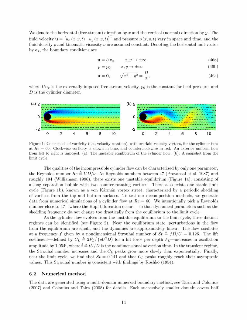
Figure 1: Color fields of vorticity (i.e., velocity rotation), with overlaid velocity vectors, for the cylinder flowat Re = 60. Clockwise vorticity is shown in blue, and counterclockwise in red. An exterior uniform flowfrom left to right is imposed. (a): The unstable equilibrium of the cylinder flow. (b): A snapshot from thelimit cycle.
The qualities of the incompressible cylinder flow can be characterized by only one parameter,the Reynolds number Re , UD/ν. At Reynolds numbers between 47 (Provansal et al. 1987) androughly 194 (Williamson 1996), there exists one unstable equilibrium (Figure 1a), consisting ofa long separation bubble with two counter-rotating vortices. There also exists one stable limitcycle (Figure 1b), known as a von Karman vortex street, characterized by a periodic sheddingof vortices from the top and bottom surfaces. To test our decomposition methods, we generatedata from numerical simulations of a cylinder flow at Re = 60. We intentionally pick a Reynoldsnumber close to 47—where the Hopf bifurcation occurs—so that dynamical parameters such as theshedding frequency do not change too drastically from the equilibrium to the limit cycle.
As the cylinder flow evolves from the unstable equilibrium to the limit cycle, three distinctregimes can be identified (see Figure 2). Near the equilibrium state, perturbations in the flowfrom the equilibrium are small, and the dynamics are approximately linear. The flow oscillatesat a frequency f given by a nondimensional Strouhal number of St , fD/U = 0.126. The liftcoefficient—defined by CL , 2FL/
(ρU2D
)for a lift force per depth FL—increases in oscillation
amplitude by 1.054t, where t , tU/D is the nondimensional advection time. In the transient regime,the Strouhal number increases and the CL peaks grow more slowly than exponentially. Finally,near the limit cycle, we find that St = 0.141 and that CL peaks roughly reach their asymptoticvalues. This Strouhal number is consistent with findings by Roshko (1954).
6.2 Numerical method
The data are generated using a multi-domain immersed boundary method; see Taira and Colonius(2007) and Colonius and Taira (2008) for details. Each successively smaller domain covers half
14

0 50 100 150 20010
−4
10−3
10−2
10−1
|CL|
(a)
0 50 100 150 2000.12
0.13
0.14
t
St
(b)
equilibrium transient cycle
Figure 2: (a): The lift coefficient magnitude as the cylinder flow evolves from the unstable equilibrium tothe limit cycle. (b): The corresponding instantaneous Strouhal number. The near-equilibrium, transient,and limit cycle regimes are indicated.
the streamwise and normal length, and samples the space twice as finely. The coarsest domainspans 48 diameters in the streamwise direction and 16 diameters in the normal direction. On thethird and finest domain, shown in Figure 1, the computational domain spans 12 diameters in thestreamwise direction and four diameters in the normal direction, with a resolution of 480 by 160pixels. In this study, we only use velocity data from this innermost domain in DMD. We use atime step of ∆t = 0.01875, which satisfies the Courant-Friedrichs-Levy condition for the numericalscheme implemented. The two references above have verified the convergence of the scheme andagreement with analytic models.
We use selective frequency damping (SFD; see Akervik et al. 2006) to solve for the unstableequilibrium. This solution is used as the initial condition of the immersed boundary solver. Becausetime derivatives are extremely small at the start of the fluid simulation, the computed equilibriumis likely close to the true equilibrium. The numerical error in the SFD solution causes the trajectoryto depart from the equilibrium, and ultimately to approach the limit cycle. Only one simulation,the one shown in Figures 1 and 2, is used in this study.
6.3 Dynamic mode decomposition of the cylinder flow
From each of the three regimes shown in Figure 2, we compute DMD on x- and y-velocity data span-ning approximately two periods of oscillation. Every 25th time step from the immersed boundarysolver is retained, so the sampling time between successive data vectors is ∆ts = 25∆t = 0.46875.The data samples from the near-equilibrium, transient, and limit cycle regimes respectively cover0 ≤ t < 15.94, 95.63 ≤ t < 111.09, and 210.94 ≤ t < 225.00. To cover two periods, we respectivelyrequire 34, 33, and 30 snapshots. Although we feed an integer number of periods into DMD, ourexperience has been that DMD is generally insensitive to this condition. This is in contrast to othermethods such as POD, which may yield nonsensical results when using non-integer periods of data.
The spectra of Ritz values are shown in Figure 3. The Strouhal number is computed by
15

−1 −0.5 0 0.5 1
−1
−0.5
0
0.5
1(a)
ℜ [λ]
ℑ[λ]
0 0.2 0.4 0.6 0.8 1
10−6
10−4
10−2
100
S t
(b)
E
−1 −0.5 0 0.5 1
−1
−0.5
0
0.5
1(c)
ℜ [λ]
0 0.2 0.4 0.6 0.8 1
10−6
10−4
10−2
100
S t
(d)
−1 −0.5 0 0.5 1
−1
−0.5
0
0.5
1(e)
ℜ [λ]
0 0.2 0.4 0.6 0.8 1
10−6
10−4
10−2
100
S t
(f)
Figure 3: Ritz values λ computed from DMD on two periods of data. Top row: as the real and imaginaryparts; the 2-norms of the corresponding Ritz vectors are indicated by the color of the circles, with darkercolors indicating greater norms. Bottom row: as the normalized vector energy E =
√m+ 1 ‖v‖2 / ‖[K xm]‖F
versus the Strouhal number. Left column: near-equilibrium regime; middle column: transient regime; rightcolumn: limit cycle regime. The arrows indicate Ritz values for which the corresponding modes are plottedin Figures 4, 6, and 7.
St = arg (λ) /(2π∆ts
), and vector energies ‖v‖2 are normalized by the root-mean-square 2-norm
of the data,∥∥[K xm
]∥∥F/√m+ 1. The most energetic mode typically has a Ritz value of λ ≈ 1.
This mode has the resemblance of (but is not exactly the same as) the mean of the data set; seeFigures 4(a, b) and 6.
In the near-equilibrium regime (Figure 3a, b), where the dynamics are nearly linear, DMDeasily recognizes the complex conjugate pair of eigenmodes primarily responsible for the oscillatingexponential growth away from the unstable equilibrium. One mode from the pair is shown inFigure 4(c–e). The spatial oscillations are the result of instabilities that convect downstream.The magnitude of complex velocity mode, as shown in Figure 4(e), attains its maximum valuefar downstream of the cylinder. The qualitative nature of this unstable mode is consistent withprevious results, such as the eigenmode analyses of Giannetti and Luchini (2007) and Marquet et al.(2008) of the linearized Navier-Stokes equations. An additional unstable pair of modes is visible inFigure 3(a, b); we posit that this is a result of numerical noise.
We momentarily skip the transient regime and discuss the limit cycle, as shown in Figure 3(e,f). The spectrum appears well-ordered; all but the least energetic modes lie very close to the unitcircle. The mode corresponding to λ = 1 (Figure 6) exhibits a shorter tail than the equivalentmode from near the equilibrium. This is expected, and is the basis of “shift mode” analyses of
16
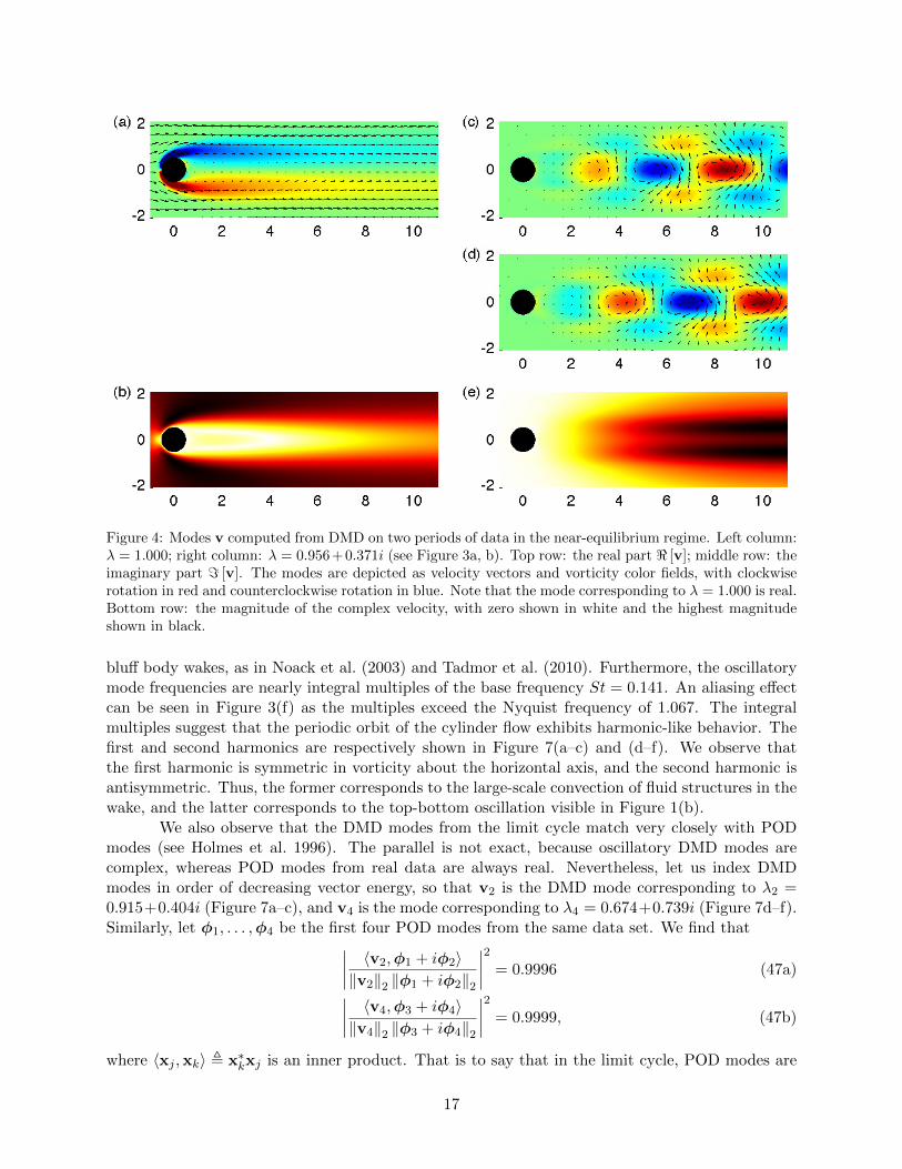
Figure 4: Modes v computed from DMD on two periods of data in the near-equilibrium regime. Left column:λ = 1.000; right column: λ = 0.956+0.371i (see Figure 3a, b). Top row: the real part < [v]; middle row: theimaginary part = [v]. The modes are depicted as velocity vectors and vorticity color fields, with clockwiserotation in red and counterclockwise rotation in blue. Note that the mode corresponding to λ = 1.000 is real.Bottom row: the magnitude of the complex velocity, with zero shown in white and the highest magnitudeshown in black.
bluff body wakes, as in Noack et al. (2003) and Tadmor et al. (2010). Furthermore, the oscillatorymode frequencies are nearly integral multiples of the base frequency St = 0.141. An aliasing effectcan be seen in Figure 3(f) as the multiples exceed the Nyquist frequency of 1.067. The integralmultiples suggest that the periodic orbit of the cylinder flow exhibits harmonic-like behavior. Thefirst and second harmonics are respectively shown in Figure 7(a–c) and (d–f). We observe thatthe first harmonic is symmetric in vorticity about the horizontal axis, and the second harmonic isantisymmetric. Thus, the former corresponds to the large-scale convection of fluid structures in thewake, and the latter corresponds to the top-bottom oscillation visible in Figure 1(b).
We also observe that the DMD modes from the limit cycle match very closely with PODmodes (see Holmes et al. 1996). The parallel is not exact, because oscillatory DMD modes arecomplex, whereas POD modes from real data are always real. Nevertheless, let us index DMDmodes in order of decreasing vector energy, so that v2 is the DMD mode corresponding to λ2 =0.915+0.404i (Figure 7a–c), and v4 is the mode corresponding to λ4 = 0.674+0.739i (Figure 7d–f).Similarly, let φ1, . . . ,φ4 be the first four POD modes from the same data set. We find that∣∣∣∣ 〈v2,φ1 + iφ2〉
‖v2‖2 ‖φ1 + iφ2‖2
∣∣∣∣2 = 0.9996 (47a)∣∣∣∣ 〈v4,φ3 + iφ4〉‖v4‖2 ‖φ3 + iφ4‖2
∣∣∣∣2 = 0.9999, (47b)
where 〈xj ,xk〉 , x∗kxj is an inner product. That is to say that in the limit cycle, POD modes are
17

Figure 5: Modes v computed from two periods of data in the transient regime. Left column: DMD mode atλ = 0.940+0.361i; right column: optimized DMD mode (m = 3) at λ = 0.940+0.378i. (See Figure 10.) Toprow: the real part < [v]; middle row: the imaginary part = [v]. Bottom row: the magnitude of the complexvelocity.
Figure 6: The DMD mode corresponding to λ = 1.000, from two periods of data in the limit cycle regime(see Figure 3e, f). (a): Velocity and vorticity color fields. (b): The magnitude of the velocity.
18

Figure 7: Modes v computed from DMD on two periods of data in the limit cycle regime. Left column:λ = 0.915 + 0.404i; right column: λ = 0.674 + 0.739i (see Figure 3e, f). Top row: the real part < [v]; middlerow: the imaginary part = [v]. Bottom row: the magnitude of the complex velocity.
0.91 0.92 0.93 0.94 0.95 0.96
0.37
0.38
0.39
0.4
0.41
ℜ [λ]
ℑ[λ]
stable unstable
equilibrium
limit cycle
Figure 8: The movement of the primary unstable Ritz value near the equilibrium (see Figures 3a and 4c–e)to the primary oscillatory Ritz value near the limit cycle (see Figures 3e and 7a–c), as a window of 16snapshots (i.e., roughly one period) traverses the cylinder data. The unit circle is shown as a solid curve,and the movement of the Ritz value is shown as a solid curve with circles.
19
extremely similar to the real and imaginary parts of DMD modes, up to a complex multiplicativefactor.
Of the three regimes, the transient one (Figure 3c, d) is the most difficult to analyze.Rowley et al. (2009) showed that the analysis of the Koopman operator, on which DMD is based,yields elegant solutions for linear dynamics and periodic dynamics. The transient regime, however,is neither. Rather, it is the part of the highly nonlinear post-Hopf-bifurcation dynamics betweenthe unstable equilibrium and the limit cycle. At Re = 60, a smooth “morphing” can be seen inthe DMD results when a window of snapshots traverses the cylinder data from the equilibrium tothe limit cycle (Figure 8). Therefore, the Ritz values and vectors are loosely between those of thenear-equilibrium regime and those of the limit cycle. For instance, compare the most energeticoscillatory mode, shown in Figure 5(a–c), to Figure 4(c–e) and Figure 7(a–c).
−1 −0.5 0 0.5 1
−1
−0.5
0
0.5
1(a)
ℜ [λ]
ℑ[λ]
0 0.2 0.4 0.6 0.8 1
10−6
10−4
10−2
100
S t
E
(b)
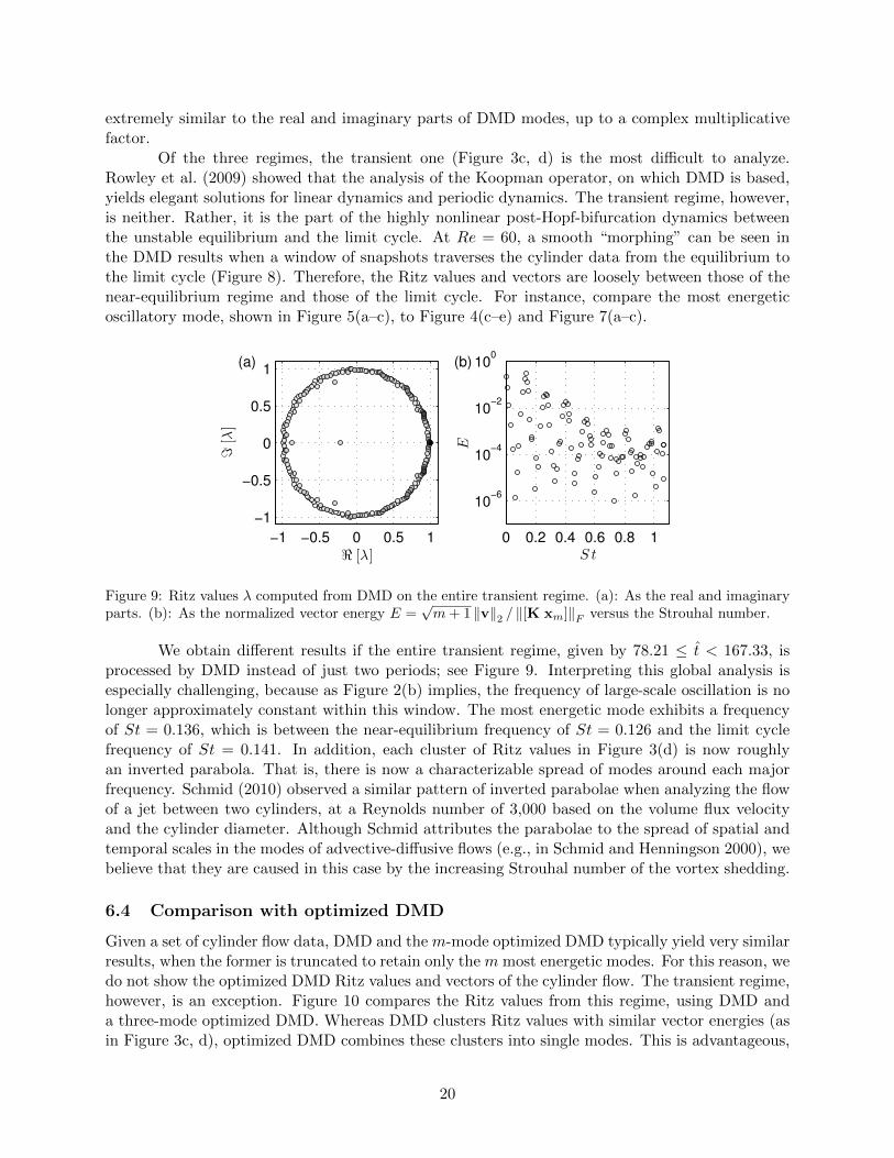
Figure 9: Ritz values λ computed from DMD on the entire transient regime. (a): As the real and imaginaryparts. (b): As the normalized vector energy E =
√m+ 1 ‖v‖2 / ‖[K xm]‖F versus the Strouhal number.
We obtain different results if the entire transient regime, given by 78.21 ≤ t < 167.33, isprocessed by DMD instead of just two periods; see Figure 9. Interpreting this global analysis isespecially challenging, because as Figure 2(b) implies, the frequency of large-scale oscillation is nolonger approximately constant within this window. The most energetic mode exhibits a frequencyof St = 0.136, which is between the near-equilibrium frequency of St = 0.126 and the limit cyclefrequency of St = 0.141. In addition, each cluster of Ritz values in Figure 3(d) is now roughlyan inverted parabola. That is, there is now a characterizable spread of modes around each majorfrequency. Schmid (2010) observed a similar pattern of inverted parabolae when analyzing the flowof a jet between two cylinders, at a Reynolds number of 3,000 based on the volume flux velocityand the cylinder diameter. Although Schmid attributes the parabolae to the spread of spatial andtemporal scales in the modes of advective-diffusive flows (e.g., in Schmid and Henningson 2000), webelieve that they are caused in this case by the increasing Strouhal number of the vortex shedding.
6.4 Comparison with optimized DMD
Given a set of cylinder flow data, DMD and the m-mode optimized DMD typically yield very similarresults, when the former is truncated to retain only the m most energetic modes. For this reason, wedo not show the optimized DMD Ritz values and vectors of the cylinder flow. The transient regime,however, is an exception. Figure 10 compares the Ritz values from this regime, using DMD anda three-mode optimized DMD. Whereas DMD clusters Ritz values with similar vector energies (asin Figure 3c, d), optimized DMD combines these clusters into single modes. This is advantageous,
20
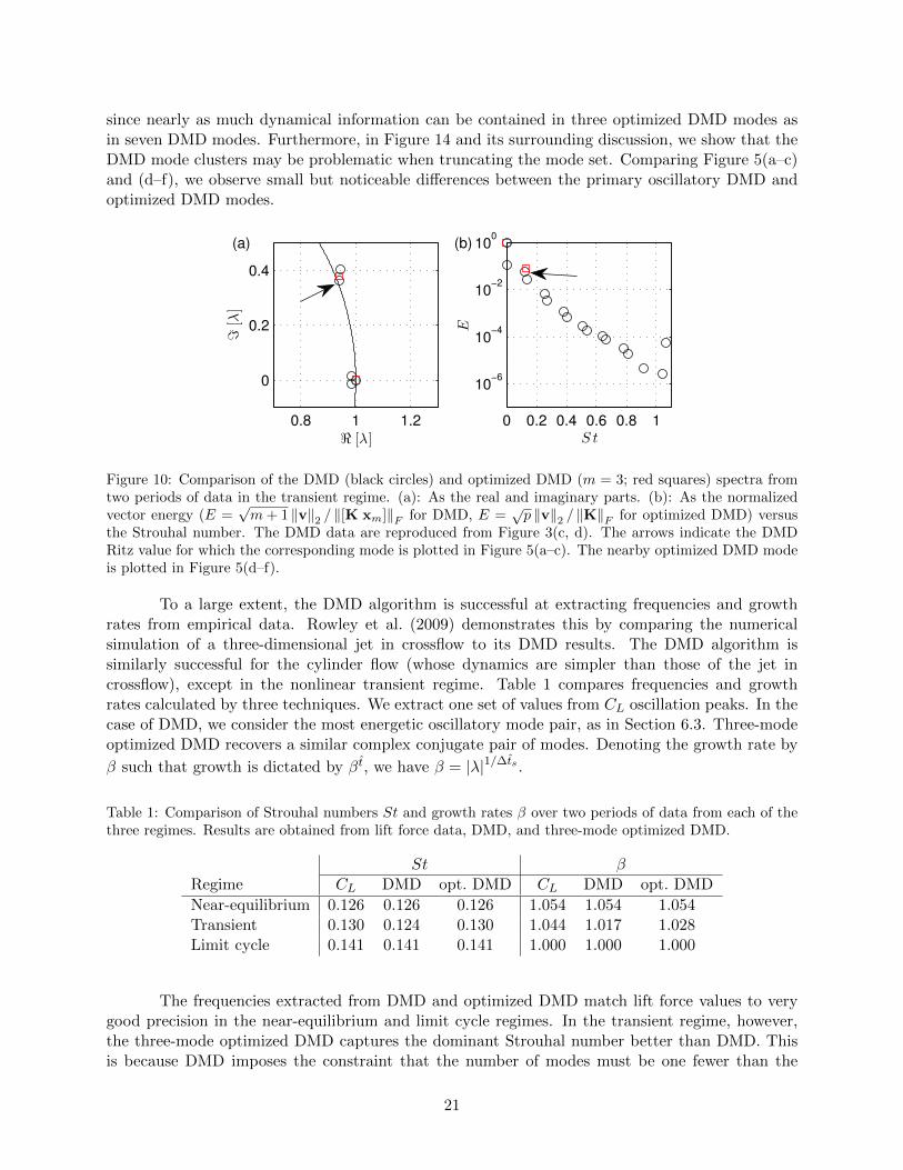
since nearly as much dynamical information can be contained in three optimized DMD modes asin seven DMD modes. Furthermore, in Figure 14 and its surrounding discussion, we show that theDMD mode clusters may be problematic when truncating the mode set. Comparing Figure 5(a–c)and (d–f), we observe small but noticeable differences between the primary oscillatory DMD andoptimized DMD modes.
0.8 1 1.2
0
0.2
0.4
(a)
ℜ [λ]
ℑ[λ]
0 0.2 0.4 0.6 0.8 1
10−6
10−4
10−2
100
S t
E
(b)
Figure 10: Comparison of the DMD (black circles) and optimized DMD (m = 3; red squares) spectra fromtwo periods of data in the transient regime. (a): As the real and imaginary parts. (b): As the normalizedvector energy (E =
√m+ 1 ‖v‖2 / ‖[K xm]‖F for DMD, E =
√p ‖v‖2 / ‖K‖F for optimized DMD) versus
the Strouhal number. The DMD data are reproduced from Figure 3(c, d). The arrows indicate the DMDRitz value for which the corresponding mode is plotted in Figure 5(a–c). The nearby optimized DMD modeis plotted in Figure 5(d–f).
To a large extent, the DMD algorithm is successful at extracting frequencies and growthrates from empirical data. Rowley et al. (2009) demonstrates this by comparing the numericalsimulation of a three-dimensional jet in crossflow to its DMD results. The DMD algorithm issimilarly successful for the cylinder flow (whose dynamics are simpler than those of the jet incrossflow), except in the nonlinear transient regime. Table 1 compares frequencies and growthrates calculated by three techniques. We extract one set of values from CL oscillation peaks. In thecase of DMD, we consider the most energetic oscillatory mode pair, as in Section 6.3. Three-modeoptimized DMD recovers a similar complex conjugate pair of modes. Denoting the growth rate by
β such that growth is dictated by β t, we have β = |λ|1/∆ts .
Table 1: Comparison of Strouhal numbers St and growth rates β over two periods of data from each of thethree regimes. Results are obtained from lift force data, DMD, and three-mode optimized DMD.
St βRegime CL DMD opt. DMD CL DMD opt. DMD
Near-equilibrium 0.126 0.126 0.126 1.054 1.054 1.054Transient 0.130 0.124 0.130 1.044 1.017 1.028Limit cycle 0.141 0.141 0.141 1.000 1.000 1.000
The frequencies extracted from DMD and optimized DMD match lift force values to verygood precision in the near-equilibrium and limit cycle regimes. In the transient regime, however,the three-mode optimized DMD captures the dominant Strouhal number better than DMD. Thisis because DMD imposes the constraint that the number of modes must be one fewer than the
21

number of data vectors. By considering only three modes, we truncate the majority of the modaldecomposition. In nonlinear dynamics, as in the transient regime, these truncated modes maycontain important information that should not be thrown out carelessly. On the other hand, thethree-mode optimized DMD tailors the decomposition to find a single complex conjugate pair ofmodes. Thus, optimized DMD provides the “best” single-frequency representation of the transientflow.
Similarly, growth rates agree near the equilibrium, where dynamics are largely linear, andnear the limit cycle, where β = 1 by definition. A larger variation is evident in the transient regime.
6.5 Comparison with the temporal DFT
−1 −0.5 0 0.5 1
−1
−0.5
0
0.5
1(a)
ℜ [λ]
ℑ[λ]
0 0.2 0.4 0.6 0.8 1
10−4
10−3
10−2
10−1
100
S t
(b)
E
−1 −0.5 0 0.5 1
−1
−0.5
0
0.5
1(c)
ℜ [λ]
0 0.2 0.4 0.6 0.8 1
10−4
10−3
10−2
10−1
100
S t
(d)
−1 −0.5 0 0.5 1
−1
−0.5
0
0.5
1(e)
ℜ [λ]
0 0.2 0.4 0.6 0.8 1
10−4
10−3
10−2
10−1
100
S t
(f)
Figure 11: Ritz values λ computed from temporal DFT on two periods of data. Top row: as the real andimaginary parts. Bottom row: as the normalized vector energy E =
√m+ 1 ‖v‖2 / ‖[K xm]‖F versus the
Strouhal number. Left column: near-equilibrium regime; middle column: transient regime; right column:limit cycle regime.
The spectra produced by the temporal DFT in each of the three data sets is shown inFigure 11. As (30) predicts, the Ritz values are exactly the m + 1 roots of unity, excluding unityitself. Therefore, to produce modes that correctly capture the large-scale features of the flow, it isimperative that the data set cover an integer number of oscillation periods. Comparing the temporalDFT vector energies to the DMD Ritz vector energies in Figure 3, we observe that the primaryoscillation modes are well-captured. These DFT modes look the same as equivalent optimizedDMD modes to the naked eye (Figures 4c–e, 5d–f, and 7).
The temporal DFT spectra, however, have a much slower decay rate. This is expected
22

in the near-equilibrium and transient regimes, since data sets there are non-periodic. The slowdecay is generally undesirable, since the implication is that a large number of modes may need tobe retained to construct an accurate solution. In addition, the low-energy modes in the transientregime are irregular and generally without meaningful physical interpretation. This is typically notthe case with low-energy DMD and optimized DMD modes.
0 5 10 150.7
0.8
0.9
1
1.1(a)
snapshots
β
0 5 10 150
0.05
0.1
0.15
0.2
0.25(b)
snapshots
St
Figure 12: The Ritz value of the limit cycle’s primary oscillatory mode, using a full period of data or less inDMD (blue line with circles) and three-mode optimized DMD (red line with pluses). A full period is 15.1snapshots. The dashed line indicates the correct value. (a): As the growth rate β. (b): As the Strouhalnumber.
An additional advantage of DMD and optimized DMD over the temporal DFT is highlightedin Figure 12. As explained in Section 4.4, the largest period that the temporal DFT can compute isthe time span of the data set. Therefore, it would have limited utility in analyzing small data setsthat cover less than a full period of oscillation. On the other hand, DMD and especially optimizedDMD are not constrained as severely. In the cylinder’s limit cycle, where a full period is 15.1snapshots, we compute DMD on two to 15 snapshots, and we compute a three-mode optimizedDMD on four to 15 snapshots. The former computes the growth rate to within a 5% error of unitywhen eight or more snapshots are used, and the latter when any number of snapshots is used.Similarly, DMD computes the Strouhal number to within a 5% error of 0.141 when nine or moresnapshots are used, and optimized DMD when eight or more are used. With only half a period ofdata, DMD can compute the modal decomposition modestly accurately; optimized DMD performseven better.
6.6 Comparison with equilibrium subtraction
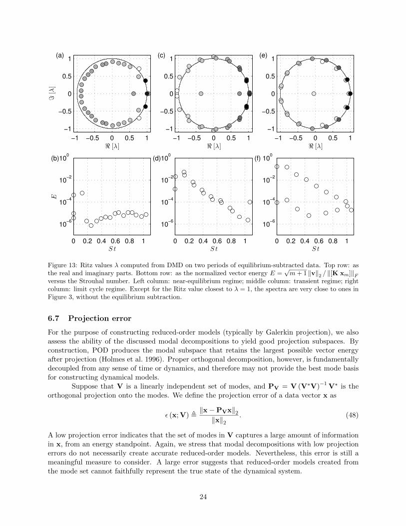
The DMD spectra of the three data sets—with the equilibrium subtracted—are shown in Figure 13.Upon comparing these spectra with the ones from the original data sets (Figure 3), we noticethat the results are nearly identical. One key difference is that the mode closest to λ = 1 is nowsignificantly weaker. This is a natural consequence of the base flow subtraction. Since the dynamicsof the cylinder flow at Re = 60 do not depart drastically from the unstable equilibrium, we couldexpect stationary DMD modes to have some resemblance to the unstable equilibrium.
To the naked eye, these DMD modes from the three regimes look identical to the modeswithout base flow subtraction; see Figures 4, 5, and 7. We stress again, however, that the baseflow subtraction is necessary to ensure that the modes have homogeneous boundary conditions.(The figures only show the innermost domain of the computational grid, and so the actual outerboundaries are not shown.)
23
−1 −0.5 0 0.5 1
−1
−0.5
0
0.5
1(a)
ℜ [λ]
ℑ[λ]
0 0.2 0.4 0.6 0.8 1
10−6
10−4
10−2
100
S t
(b)
E
−1 −0.5 0 0.5 1
−1
−0.5
0
0.5
1(c)
ℜ [λ]
0 0.2 0.4 0.6 0.8 1
10−6
10−4
10−2
100
S t
(d)
−1 −0.5 0 0.5 1
−1
−0.5
0
0.5
1(e)
ℜ [λ]
0 0.2 0.4 0.6 0.8 1
10−6
10−4
10−2
100
S t
(f)
Figure 13: Ritz values λ computed from DMD on two periods of equilibrium-subtracted data. Top row: asthe real and imaginary parts. Bottom row: as the normalized vector energy E =
√m+ 1 ‖v‖2 / ‖[K xm]‖F
versus the Strouhal number. Left column: near-equilibrium regime; middle column: transient regime; rightcolumn: limit cycle regime. Except for the Ritz value closest to λ = 1, the spectra are very close to ones inFigure 3, without the equilibrium subtraction.
6.7 Projection error
For the purpose of constructing reduced-order models (typically by Galerkin projection), we alsoassess the ability of the discussed modal decompositions to yield good projection subspaces. Byconstruction, POD produces the modal subspace that retains the largest possible vector energyafter projection (Holmes et al. 1996). Proper orthogonal decomposition, however, is fundamentallydecoupled from any sense of time or dynamics, and therefore may not provide the best mode basisfor constructing dynamical models.
Suppose that V is a linearly independent set of modes, and PV = V (V∗V)−1 V∗ is theorthogonal projection onto the modes. We define the projection error of a data vector x as
ε (x; V) ,‖x−PVx‖2‖x‖2
. (48)
A low projection error indicates that the set of modes in V captures a large amount of informationin x, from an energy standpoint. Again, we stress that modal decompositions with low projectionerrors do not necessarily create accurate reduced-order models. Nevertheless, this error is still ameaningful measure to consider. A large error suggests that reduced-order models created fromthe mode set cannot faithfully represent the true state of the dynamical system.
24
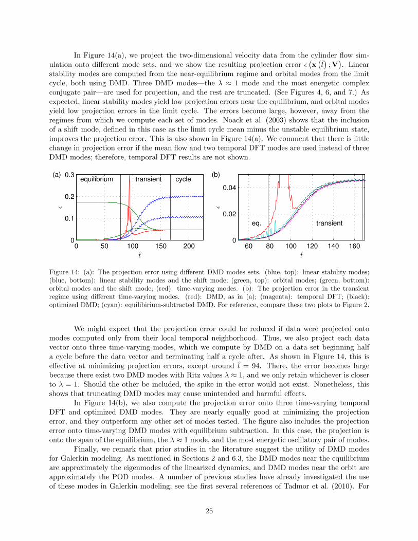
In Figure 14(a), we project the two-dimensional velocity data from the cylinder flow sim-ulation onto different mode sets, and we show the resulting projection error ε
(x(t)
; V). Linear
stability modes are computed from the near-equilibrium regime and orbital modes from the limitcycle, both using DMD. Three DMD modes—the λ ≈ 1 mode and the most energetic complexconjugate pair—are used for projection, and the rest are truncated. (See Figures 4, 6, and 7.) Asexpected, linear stability modes yield low projection errors near the equilibrium, and orbital modesyield low projection errors in the limit cycle. The errors become large, however, away from theregimes from which we compute each set of modes. Noack et al. (2003) shows that the inclusionof a shift mode, defined in this case as the limit cycle mean minus the unstable equilibrium state,improves the projection error. This is also shown in Figure 14(a). We comment that there is littlechange in projection error if the mean flow and two temporal DFT modes are used instead of threeDMD modes; therefore, temporal DFT results are not shown.
0 50 100 150 2000
0.1
0.2
0.3
t
ǫ
equilibrium transient cycle(a)
60 80 100 120 140 1600
0.02
0.04
t
ǫeq. transient
(b)
Figure 14: (a): The projection error using different DMD modes sets. (blue, top): linear stability modes;(blue, bottom): linear stability modes and the shift mode; (green, top): orbital modes; (green, bottom):orbital modes and the shift mode; (red): time-varying modes. (b): The projection error in the transientregime using different time-varying modes. (red): DMD, as in (a); (magenta): temporal DFT; (black):optimized DMD; (cyan): equilibirium-subtracted DMD. For reference, compare these two plots to Figure 2.
We might expect that the projection error could be reduced if data were projected ontomodes computed only from their local temporal neighborhood. Thus, we also project each datavector onto three time-varying modes, which we compute by DMD on a data set beginning halfa cycle before the data vector and terminating half a cycle after. As shown in Figure 14, this iseffective at minimizing projection errors, except around t = 94. There, the error becomes largebecause there exist two DMD modes with Ritz values λ ≈ 1, and we only retain whichever is closerto λ = 1. Should the other be included, the spike in the error would not exist. Nonetheless, thisshows that truncating DMD modes may cause unintended and harmful effects.
In Figure 14(b), we also compute the projection error onto three time-varying temporalDFT and optimized DMD modes. They are nearly equally good at minimizing the projectionerror, and they outperform any other set of modes tested. The figure also includes the projectionerror onto time-varying DMD modes with equilibrium subtraction. In this case, the projection isonto the span of the equilibrium, the λ ≈ 1 mode, and the most energetic oscillatory pair of modes.
Finally, we remark that prior studies in the literature suggest the utility of DMD modesfor Galerkin modeling. As mentioned in Sections 2 and 6.3, the DMD modes near the equilibriumare approximately the eigenmodes of the linearized dynamics, and DMD modes near the orbit areapproximately the POD modes. A number of previous studies have already investigated the useof these modes in Galerkin modeling; see the first several references of Tadmor et al. (2010). For
25

a comprehensive study specifically relating to the Galerkin modeling of the cylinder wake, referto Noack et al. (2003); this particular study shows that the wake is accuracy modeled using acombination of POD modes, linear stability modes, and the shift mode.
7 Conclusion
The Koopman operator is a linear operator that represents nonlinear dynamics without lineariza-tion. Dynamic mode decomposition is a data-based method for estimating Koopman eigenvaluesand modes. It approximates a dynamical trajectory, often generated by a nonlinear system, as theresult of a linear process. The Ritz values of the decomposition yield growth rates and frequencies,and the Ritz vectors yield corresponding directions. Unlike many previous decomposition tech-niques such as POD and balanced POD, DMD is not tightly constrained; the data need be neitherperiodic nor linearly generated for DMD to construct a meaningful modal decomposition.
We prove that the DMD algorithm of Rowley et al. (2009) and Schmid (2010) producesa unique decomposition if and only if all vectors except the last in a given data set are linearlyindependent, and the Ritz values are distinct. If either condition is violated, then non-unique Ritzvalues and vectors may still exist.
To use DMD modes in a reduced-order Galerkin model of a partial differential equation,a “base flow” that satisfies the appropriate boundary conditions must typically be included. Themean of the data is a common choice for a base flow, especially in POD-based analyses. Dynamicmode decomposition on a mean-subtracted set of data, however, is exactly equivalent to a temporalDFT and harmonic averaging. This implies that for m+1 data vectors, the Ritz values are preciselythe m + 1 roots of unity, excluding unity itself. The inability to compute growth rates, as well asthe predetermination of frequencies regardless of data content, are fundamental properties of thetemporal DFT. In addition, the temporal DFT cannot capture a particular frequency if the dataset covers less than one corresponding period. Furthermore, the decay of temporal DFT vectorenergies is slow if the data are non-periodic. We can avoid these issues by choosing the equilibriumpoint instead as the base flow.
Next, we introduce an optimized DMD, in which the decomposition is tailored specifically tothe desired number of output modes. In this decomposition, the representation of any data vectormay contain a residual, but the total residual over all data vectors is minimized. In the absenceof an analytic algorithm, we use simulated annealing and quasi-Newton iterators to compute theoptimized DMD. Aside from these iterators, this decomposition generally does not suffer fromnumerical sensitivity as DMD does. Optimized DMD is also superior for computing a small numberof modes, since the decomposition is computed for the given number of modes and does not requirearbitrary truncation.
The two-dimensional incompressible flow over a cylinder is used as a test bed for the afore-mentioned decomposition methods. Dynamic mode decomposition recovers the leading unstableeigenmodes from data near the unstable equilibrium. It also recovers POD-like modes from datanear the limit cycle. When a small window of snapshots traverses the cylinder data from theequilibrium to the limit cycle, the Ritz values and vectors morph gradually.
The optimized DMD and equilibrium-subtracted DMD of the cylinder flow reproduce theDMD results to a large extent. A significant improvement can be seen in the transient regime,however. Optimized DMD computes growth rates and frequencies more faithfully, and it avoidsclusters of Ritz values, which are problematic for truncating mode sets. Equilibrium-subtractedDMD, on the other hand, largely preserves the DMD modes and spectra, while correctly accountingfor boundary conditions. Temporal DFT modes of the cylinder flow look qualitatively like optimized
26

DMD modes, but the roll-off in the Ritz vector energies is slow when data are not taken from theperiodic orbit. Unlike the temporal DFT, DMD is able to compute frequencies and growth ratesfrom little over half a period of data; optimized DMD fares even better.
As the cylinder flow evolves from the unstable equilibrium to the stable limit cycle, time-varying temporal DFT, optimized DMD, and equilibrium-subtracted DMD modes are better able torepresent data (in the sense of energy) than time-varying DMD modes. These mode sets maintaina low error through the entire trajectory of the cylinder flow, from the equilibrium to the limitcycle. Based on these findings, we hypothesize that the use of these time-varying modes may yieldaccurate Galerkin models.
Acknowledgements
This work was supported by the Department of Defense National Defense Science & EngineeringGraduate (DOD NDSEG) Fellowship, the National Science Foundation Graduate Research Fellow-ship Program (NSF GRFP), and AFOSR grant FA9550-09-1-0257.
References
E. Akervik, L. Brandt, D. S. Henningson, J. Hœpffner, O. Marxen, and P. Schlatter. Steadysolutions of the Navier-Stokes equations by selective frequency damping. Phys. Fluids, 18(6):068102, 2006.
T. Colonius and K. Taira. A fast immersed boundary method using a nullspace approach and multi-domain far-field boundary conditions. Comput. Meth. Appl. Mech. Eng., 197(25–28):2131–2146,2008.
F. Giannetti and P. Luchini. Structural sensitivity of the first instability of the cylinder wake. J.Fluid Mech., 581:167–197, 2007.
E. A. Gillies. Low-dimensional control of the circular cylinder wake. J. Fluid Mech., 371:157–178,1998.
P. Holmes, J. L. Lumley, and G. Berkooz. Turbulence, Coherent Structures, Dynamical Systemsand Symmetry. Cambridge University Press, 1996.
M. Ilak and C. W. Rowley. Modeling of transitional channel flow using balanced proper orthogonaldecomposition. Phys. Fluids, 20(3):034103, 2008.
O. Marquet, D. Sipp, and L. Jacquin. Sensitivity analysis and passive control of cylinder flow. J.Fluid Mech., 615:221–252, 2008.
I. Mezic. Spectral properties of dynamical systems, model reduction and decompositions. NonlinearDyn., 41(1–3):309–325, 2005.
I. Mezic and A. Banaszuk. Comparison of systems with complex behavior. Physica D, 197(1–2):101–133, 2004.
B. C. Moore. Principal component analysis in linear systems: controllability, observability, andmodel reduction. IEEE Trans. Autom. Control, 26(1):17–32, 1981.
27
B. R. Noack, K. Afanasiev, M. Morzynski, G. Tadmor, and F. Thiele. A hierarchy of low-dimensionalmodels for the transient and post-transient cylinder wake. J. Fluid Mech., 497:335–363, 2003.
B. R. Noack, P. Papas, and P. A. Monkewitz. The need for a pressure-term representation inempirical Galerkin models of incompressible shear flow. J. Fluid Mech., 523:339–365, 2005.
K. Petersen. Ergodic Theory. Cambridge University Press, 1983.
W. H. Press, S. A. Teukolsky, W. T. Vetterling, and B. P. Flannery. Numerical Recipes. CambridgeUniversity Press, 3rd edition, 2007.
M. Provansal, C. Mathis, and L. Boyer. Benard-von Karman instability: transient and forcedregimes. J. Fluid Mech., 182:1–22, September 1987.
A. Roshko. On the development of turbulent wakes from vortex streets. Technical Report NACA1191, National Advisory Committee for Aeronautics, 1954.
K. Roussopoulos. Feedback control of vortex shedding at low Reynolds numbers. J. Fluid Mech.,248:267–296, 1993.
C. W. Rowley. Model reduction for fluids, using balanced proper orthogonal decomposition. Int.J. Bifurc. Chaos, 15(3):997–1013, 2005.
C. W. Rowley, I. Mezic, S. Bagheri, P. Schlatter, and D. S. Henningson. Spectral analysis ofnonlinear flows. J. Fluid Mech., 641:115–127, 2009.
P. J. Schmid. Dynamic mode decomposition of numerical and experimental data. J. Fluid Mech.,656:5–28, 2010.
P. J. Schmid. Application of the dynamic mode decomposition to experimental data. Exp. Fluids,50(4):1123–1130, 2011.
P. J. Schmid and D. S. Henningson. Stability and Transition in Shear Flows. Springer, 2000.
P. J. Schmid, L. Li, M. P. Juniper, and O. Pust. Applications of the dynamic mode decomposition.Theor. Comput. Fluid Dyn., 25(1–4):249–259, 2011.
G. Tadmor, O. Lehmann, B. R. Noack, and M. Morzynski. Mean field representation of the naturaland actuated cylinder wake. Phys. Fluids, 22(3):034102, 2010.
K. Taira and T. Colonius. The immersed boundary method: a projection approach. J. Comput.Phys., 225(2):2118–2137, 2007.
C. H. K. Williamson. Vortex dynamics in the cylinder wake. Annu. Rev. Fluid Mech., 28:477–539,1996.
28