Variation in Assemblies

• Goals of this class – Understand how to represent variation at the assembly

level – Link models to models of variation at the part level– Link models to nominal chain of frames – Get an idea of statistical process control and statistical

tolerancing vs worst case tolerancing

© Daniel E Whitney

History of Tolerances in Assemblies

• Statistical process control and statistical tolerancing permit a bet on interchangeability

• Coordination makes a comeback as functional build

• Quality today is more than interchangeability – The product almost certainly will “work” – Real quality means

• Durability • Reliability • Low noise, vibration, etc

– All are associated with low running clearances, fine balance, etc., all requiring closer tolerances, robust design, etc.

© Daniel E Whitney

Recent Gains in Productivity• Wall Street Journal, Sept 28, 00, p 2:

– “Many analysts may have overlooked one of the main drivers of the productivity gains of the last five years: machine tools… more than half the increase has occurred outside the computer, software, and telecommunications sectors...

– Greater precision in machine tools has helped cut the energy use of air conditioners by 10% between 1990 and 1997 … using a new kind of compressor whose manufacture required … precision down to 10 microns”

– One of the principal reasons for more reliable automobile transmissions ...

– Open architecture, digital programming, ceramic tool bits are part of the picture

© Daniel E Whitney

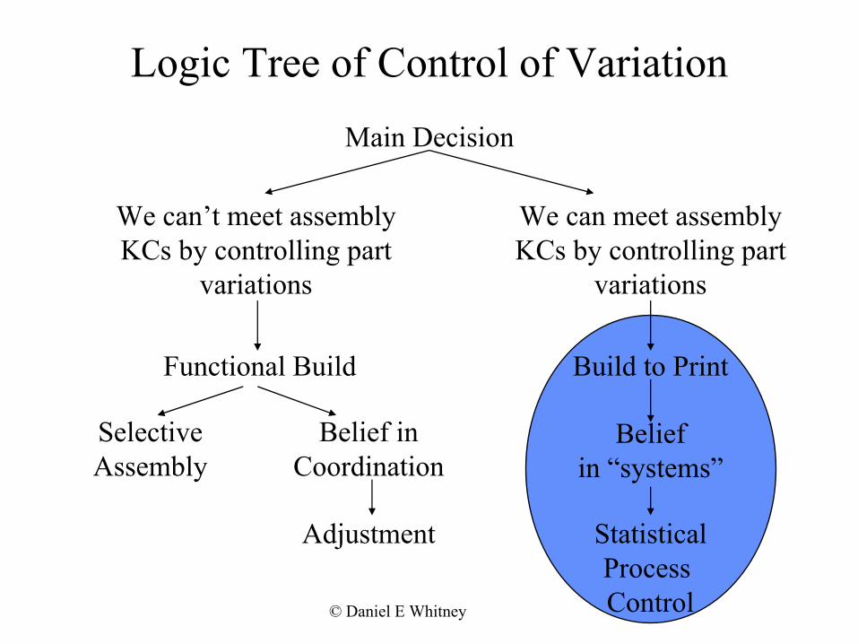
Logic Tree of Control of Variation

Main Decision

We can’t meet assemblyKCs by controlling part

variations

We can meet assemblyKCs by controlling part

variations

Functional Build

Selective Belief inAssembly Coordination

Adjustment

© Daniel E Whitney

Build to Print

Statistical Process Control

Belief in “systems”

Two Kinds of Errors

• Change in process average (mean shift) • Process variation around the mean (variance)• These are different kinds of errors that require

different approaches – The screwdriver workstation-RCC story – Whitehead’s reason for using kinematic design

– Taguchi’s systematic approach • Correct mean shift first, then reduce variation

© Daniel E Whitney

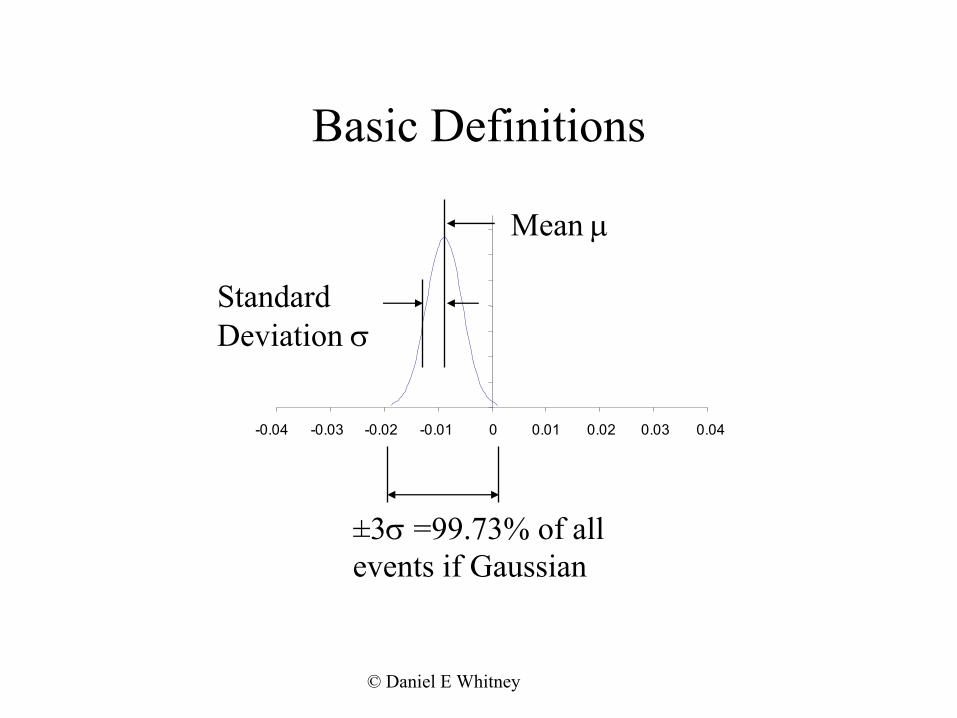
Basic Definitions

Mean µ

Standard Deviation σ

-0.04 -0.03 -0.02 -0.01 0 0.01 0.02 0.03 0.04

±3σ =99.73% of allevents if Gaussian

© Daniel E Whitney

Precision vs Accuracy

USLLSL USL LSL

Desired tolerance

σ

Desired tolerance

σ

bandband

Distribution of Distribution of actual process actual process results results

-0.04 -0.03 -0.02 -0.01 0 0.01 0.02 0.03 0.04 -0.04 -0.03 -0.02 -0.01 0 0.01 0.02 0.03 0.04

Process mean µ Desired value Desired value = µ

Consistent but consistently wrong Right on the average

© Daniel E Whitney

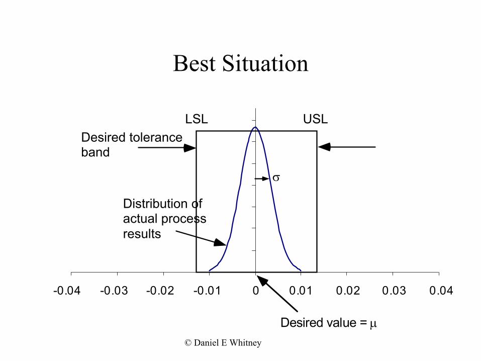
Best Situation

Desired tolerance

Distribution ofactual process

-0.04 -0.03 -0.02 -0.01 0 0.01 0.02 0.03 0.04

Desired value = µ

σ

© Daniel E Whitney

LSL USL

band

results

Models of How Errors Accumulate in Assemblies

• Worst case tolerancing – Assumes all errors are at their extremes at the same time – This is deterministic, not statistical – Errors accumulate linearly with the number of parts

• Statistical tolerancing (AKA root sum square) – Assumes errors are distributed randomly ± between limits – Errors accumulate with SQRT of number of parts but only

if the average part error = the desired nominal dimension! (i.e., average part (& assy) error = 0.)

© Daniel E Whitney

A N V I L

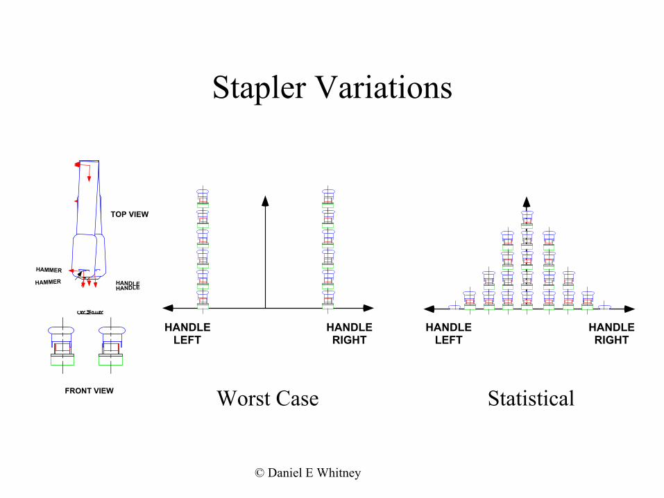
R I V E T Stapler Variations

TOP VIEW

HANDLEHANDLE

HAMMER

HAMMER HANDHANDLELE

C R I M P E R

HANDLE HANDLE LEFT RIGHT LEFT RIGHT

FRONT VIEW Worst Case Statistical

© Daniel E Whitney

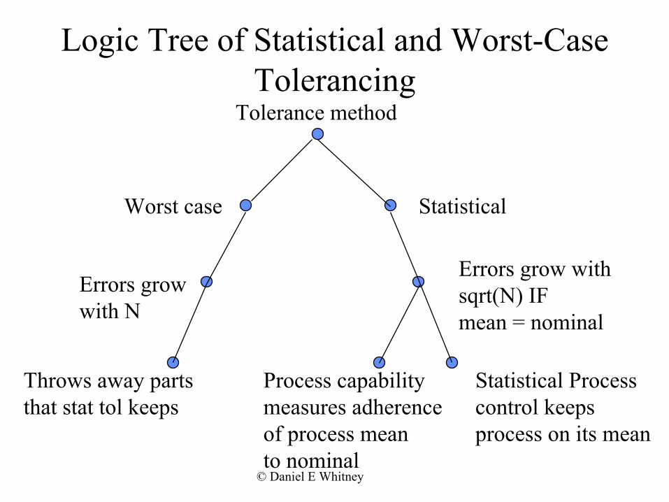
Logic Tree of Statistical and Worst-Case Tolerancing

Tolerance method

Worst case Statistical

Errors grow withErrors grow sqrt(N) IFwith N mean = nominal

Throws away partsthat stat tol keeps

Process capability measures adherence of process mean to nominal

© Daniel E Whitney

Statistical Process control keeps process on its mean

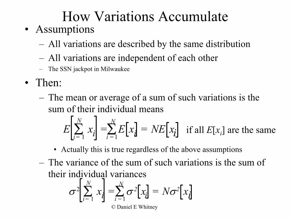
How Variations Accumulate• Assumptions

– All variations are described by the same distribution – All variations are independent of each other – The SSN jackpot in Milwaukee

• Then: – The mean or average of a sum of such variations is the

sum of their individual means N

E Σi = 1

N =xi Σ

i = 1 E xi = NE if all E[xi] are the same xi

• Actually this is true regardless of the above assumptions

– The variance of the sum of such variations is the sum of their individual variances

N σ 2 Σ

i = 1 xi Σ

i = 1

N σ 2

© Daniel E Whitney

2Nσ xi= xi =

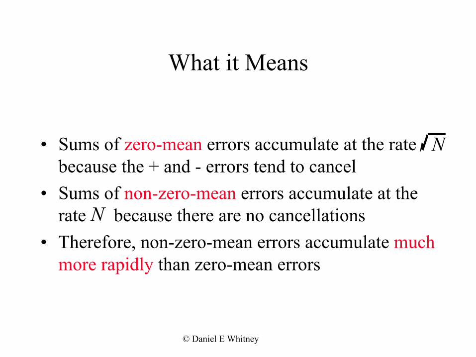
What it Means

• Sums of zero-mean errors accumulate at the rate N because the + and - errors tend to cancel

• Sums of non-zero-mean errors accumulate at the rate N because there are no cancellations

• Therefore, non-zero-mean errors accumulate much more rapidly than zero-mean errors

© Daniel E Whitney

Why the Mean Should Seek the Nominal

99.73% of Error if Mean = 0

99.73% of Error if Mean ° 0

Number of Parts or Events

Accumulated Error

3σ envelope

How to survive Las Vegas © Daniel E Whitney

RSS (Root Sum Square) Method

Li = L0i + xi

xi = mi + ρi

where the average of ρi = ρ = 0

and the variance of ρ = σi 2

i

n n n 2RSS Error in ∑Li = ∑(Error in Li )2 = = σ∑σ i = σ n if σ i

i =1 i=1 i =1

RSS method is valid only if mi = 0

© Daniel E Whitney

© Dani

Statistical and Worst Case Compared for Three Additive TolerancesWorst case Statistical

el E Whitney

0

0

i

i ) / 3 i

pk > 1 3

3σ

3σ

0

0

i

91.6% of these are within ±0.01

Indi

vidu

al P

arts

Asse

mbl

ies

LSL USL

LSL USL LSL USL

LSL USL

-0. 04 -0.03 -0.02 -0.01 0.01 0.02 0.03 0.04

-0.04 -0.0 3 -0.02 -0.01 0.01 0.02 0.03 0.04

Des red final tolerance = ±0.03 0.27% of assemblies will exceed ±0.03

3 parts are toleranced at ±0.01 each = (f nal tol and inspected 100%

3 parts are toleranced at ±0.01732 each = (f nal tol ) / and not inspected if C

All assemblies will be in this range

All parts will be in this range

-0.04 -0.03 -0.02 -0.01 0.01 0.02 0.03 0.04

-0.04 -0.03 -0.02 -0.01 0.01 0.02 0.03 0.04

Des red final tolerance = ±0.03 0.00% of assemblies will exceed ±0.03

pa r t

t o t a l

Process Capability• Every process has a mean and a “natural tolerance” range

• Process capability indiex Cpk tracks whether the process range is within the 3σ tolerance band and the process mean is on the target nominal dimension

USL − X LSL − X Cpk = min ;

3σ

3σ

USL = upper spec (tolerance) limit LSL = lower spec (tolerance) limit X = mean of the process σ = variance of the process

© Daniel E Whitney

- 4

Process Capability CpkActual error

Cpk = 0.667

Cpk = 1

pk

Cpk = 0.667

If this is the tolerance band, then C = 1.33

Units of σ - 3 - 2 - 1 0 1 2 3 4

# of σ % within ±# of σ % outside 1 68.269% 31.731% 2 95.450% 4.550% 3 99.730% 0.270% 4 99.994% 0.006%

© Daniel E Whitney

Process Control & Capability

© Daniel E Whitney

Effect of Mean Shift0.00167 shift in each part

3σ=.01732

-0.04 -0.03 -0.02 -0.01 0 0.01 0.02 0.03 0.04

0

2.5σ

1.24% will exceed 0.03

Range % Outside ± 1 sigma 31.74 ± 2 sigma 4.54% ± 2.5 sigma 1.24% ± 3 sigma 0.27%

.005 total shift in 3 parts=0.5σ

3σ=.03

-0.04 -0.03 -0.02 -0.01 0.01 0.02 0.03 0.04

Cpk=1.00 Cpk=.833

© Daniel E Whitney

How Could Non-zero Mean Variations Occur?

• For material removal processes, operators stop as soon as the part enters the tolerance zone from the high side

• For material-adding processes, operators stop as soon as the part enters the zone from the low side

Desired mean

Actual mean

Tolerance zone

Desired mean

Actual mean

Tolerance zone

Original size of material

Material being Material being cut to size built-up to size

Original size of material

Removal Process Additive Process© Daniel E Whitney

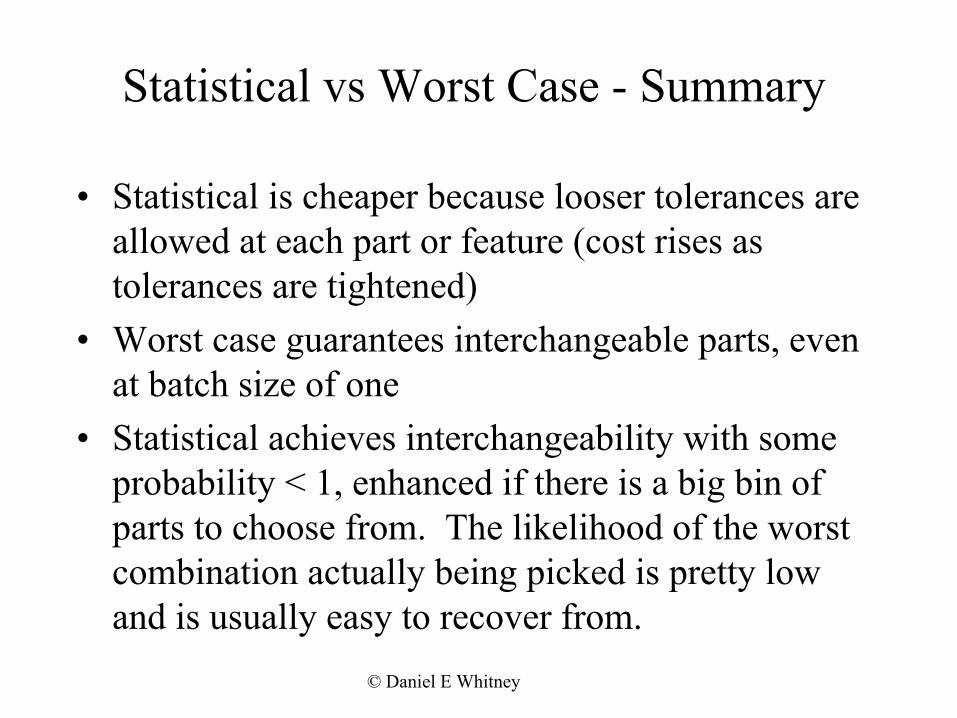
Statistical vs Worst Case - Summary

• Statistical is cheaper because looser tolerances are allowed at each part or feature (cost rises as tolerances are tightened)

• Worst case guarantees interchangeable parts, even at batch size of one

• Statistical achieves interchangeability with some probability < 1, enhanced if there is a big bin of parts to choose from. The likelihood of the worst combination actually being picked is pretty low and is usually easy to recover from.

© Daniel E Whitney

© Daniel E Whitney

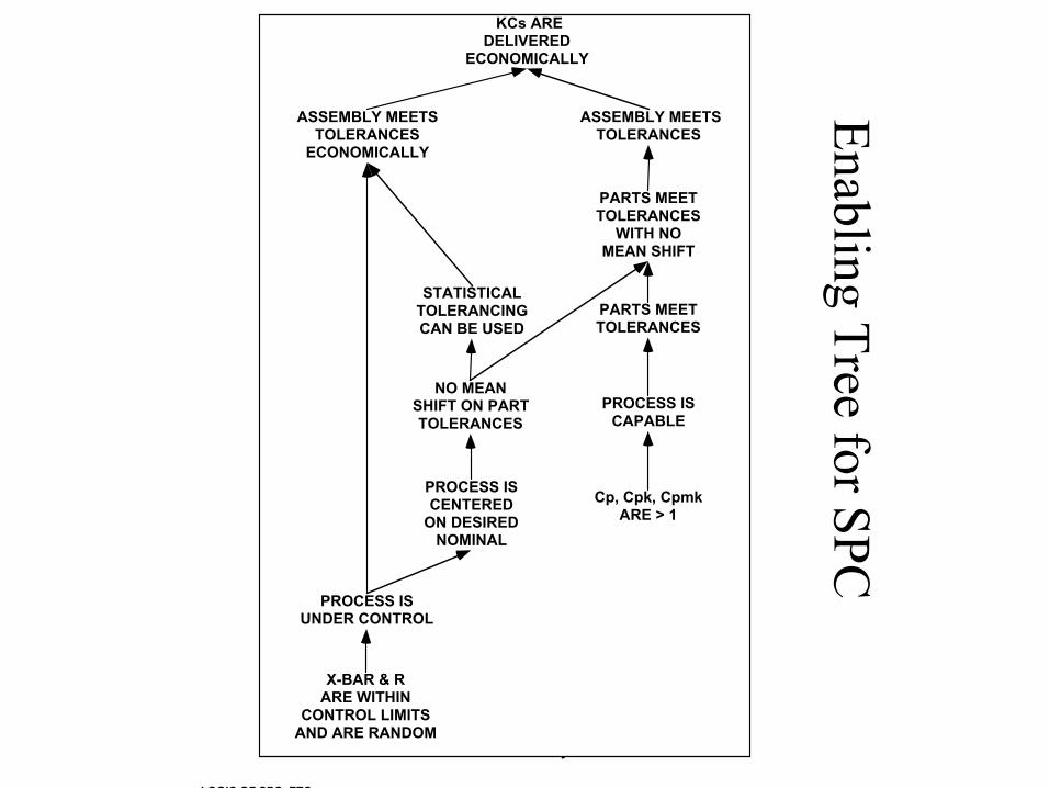
Enabling Tree for SPC

KCs ARE DELIVERED

ECONOMICALLY

ASSEMBLY MEETS TOLERANCES

ASSEMBLY MEETS TOLERANCES

ECONOMICALLY

NO MEAN SHIFT ON PART TOLERANCES

PARTS MEET TOLERANCES

X-BAR & R ARE WITHIN

CONTROL LIMITS AND ARE RANDOM

PROCESS IS UNDER CONTROL

PROCESS IS CAPABLE

PROCESS IS CENTERED

ON DESIRED NOMINAL

Cp, Cpk, CpmkARE > 1

STATISTICAL TOLERANCING CAN BE USED

PARTS MEET TOLERANCES

WITH NO MEAN SHIFT

LOGIC OF SPC ETC

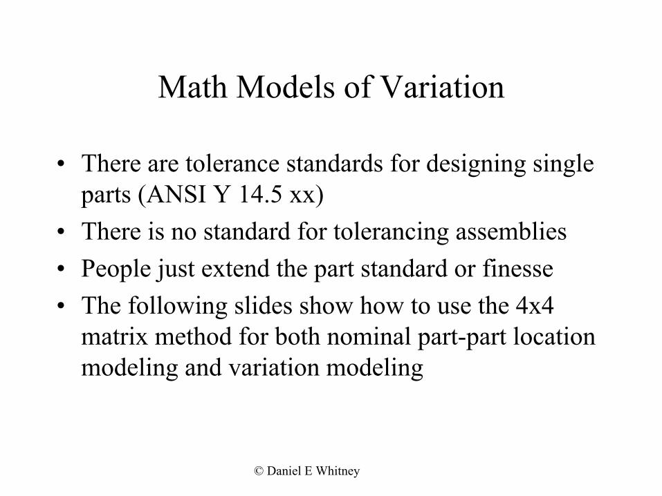
Math Models of Variation

• There are tolerance standards for designing single parts (ANSI Y 14.5 xx)

• There is no standard for tolerancing assemblies

• People just extend the part standard or finesse

• The following slides show how to use the 4x4 matrix method for both nominal part-part location modeling and variation modeling

© Daniel E Whitney

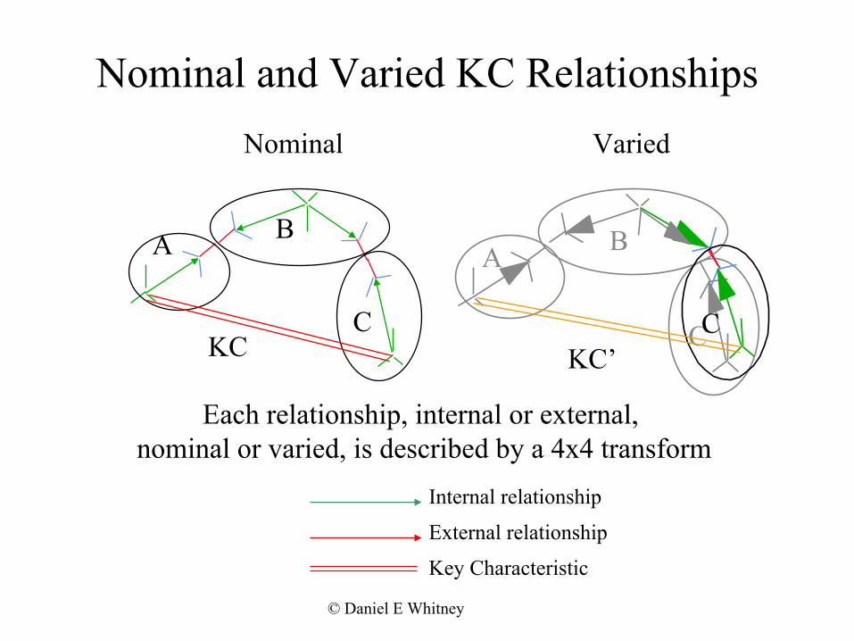
Nominal and Varied KC Relationships

Nominal Varied

A B

C KC C

A B

C KC’

Each relationship, internal or external, nominal or varied, is described by a 4x4 transform

Internal relationship

External relationship

Key Characteristic

© Daniel E Whitney

(c) 1985 MIT Press. p. 442.

Engine Cross Section

© Daniel E Whitney

Taylor, C.F. Figure 11-8 of THE INTERNAL COMBUSTION ENGINE IN THEORY AND PRACTICE,

volume 2, revised edition. (c) 1985 MIT Press. p. 442.

Chain of Frames for Engine

Cylinder Head

Cam Shaft

Lifter

Valve

Cylinder Block

Crankshaft

Connecting Rod

Piston

Wrist Pin

Timing Chain

KC

Cylinder

CamDon’t forget the head gasket!

Statistical tolerancing can delivers this KC

© Daniel E Whitney

Valve and Lifter Use Selective Assembly

The ones used today

The ones used another day

Cylinder Head

Cam Shaft

Lifter

Valve

KC

Cam

lected

Li

Cam Statistical Tolerancing cannot deliver this KCSe

Solid fter

Cylinder Head

Valve

50 Bins Covering 200µ total

© Daniel E Whitney

How Selective Assembly is Done

Clearance is

Shaft

Normal Distribution

0.5

0

0.1

0.2

0.3

0.4

-4 -3 -2 -1 0 1 2 3 4

x

Bearing

Pick and measure a shaft. important

If it is a bit big, pick a big bearing to get clearance right. If it is a bit small, pick a small bearing. For this to work over a long stretch, there must be about the same number of big shafts as big bearings, and the same for small ones.

© Daniel E Whitney

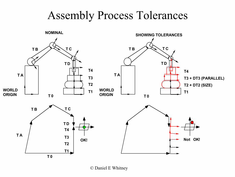
Assembly Process TolerancesNOMINAL SHOWING TOLERANCES

T B T C

T D T4

T B T C

T D

T4 T AT A T3 T3 + DT3 (PARALLEL)

T2 T2 + DT2 (SIZE) WORLD T1 WORLD T1ORIGIN ORIGINT 0 T 0

T A

T1

T2 T3

T4

T B T C

T D

Not OK! OK!

T 0

© Daniel E Whitney

Nominal Mating of Parts

TAF

A T

FB

B

Parts A and B are mated by joining two features

T T

T

AF

FB

AB

A

B

The nominal location of part B can be calculated from the nominal location of part A using 4x4 transform math

© Daniel E Whitney

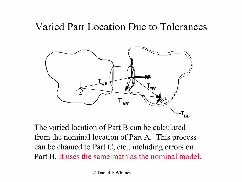
Varied Part Location Due to Tolerances

T T

T

AF FB'

AB'

A B'

TBB'

The varied location of Part B can be calculated from the nominal location of Part A. This process can be chained to Part C, etc., including errors on Part B. It uses the same math as the nominal model.

© Daniel E Whitney

Equations for Connective Models

Feature A Feature B

Part BTA-FA TFA-FB

TFB-BNominal

Part A

Part A Feature A

Feature B

TA-FA

TFB-B

Feature A'

DTFA-FA' DTFA'-FA"

DTFA-FB Part BTFA-FB

Feature A"

Varied

Feature Feature

Interface (clearance)

shapelocation

© Daniel E Whitney

Error Transform (Linearized)

dθ1 δθ z

–δθ y

0

– δθz δθ y

1 –δθ x

δθ x 1 0 0

dx dy dz 1

T’ = T * DT T DTT’

dp

DT =

© Daniel E Whitney

Transform Order is Important

T=DT11’T12

This is a frame 1 event

2T12

DT 22’

DT11’ This is a frame 2 event

1Tells us what T=T12DT22’everything looks like from frame 1’s pov Moves the focus to frame 2 and

converts frame 2 events to frame 1 coords.

© Daniel E Whitney

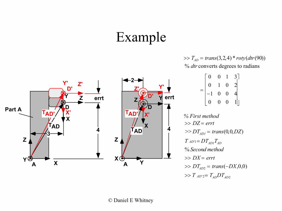
Example>> TAD = trans(3, 2,4) * roty(dtr (90)) % dtr converts degrees to radians

0 0 1 3

Z

Y

X

Z D

Y

4 TAD 3

Y'

X'

Z' D'

TAD'

errt

4X

Z Y D

X

Z

2

X'

Z' Y' D'

TAD'

TAD

errt 0 1 0 2

= −1 0 0 4

0 0 0 1

Part A % First method >> DZ = errt >> DTAD1 = trans(0,0,DZ)

T AD'1 = DTAD1TAD

% Second method >> DX = errt

A X A Y >> DTAD2 = trans(−DX ,0,0) >> T AD' 2 = TADDTAD2

© Daniel E Whitney

Example - 2

X

ZY E

F

TEF

2

X'

Z'Y'

E'

X

Y

TEF

F

7

2

>> TEF = trans (6,0,1)Part B

1

=

1 0 0 6 0 1 0 0 0 0 1 1 0 0 0 1

>> TEE ' = roty (dtr (−erra)) >> TE = roty (dtr (erra)) >> T

'E

E 'F = TE 'ETEF

© Daniel E Whitney

1

Example - 3

X

ZE

F

TEF

2

X'

Z'

E'

Part B'

X

Z

Y

X'

Z'D'

T AD'Part A'

>> TDE = rotz (dtr (180)) −1 0 0 0 0 −1 0 0

0 0 0 1

=0 0 1 0

>> TAF = TADTDETEF

0 0 0 −1 0 1 0 10

1 4

=0

0 0

%T>> T 'AF = TAD 'TD ' E 'TE 'F

D' E ' = TDE

0 1

A

© Daniel E Whitney

2

Constructing Matrix Representations of GD&T

© Daniel E Whitney

Position and Angle are Coupled by Rule #1

θ x z

θ x)f(z,

z

θ

S

/ LS

TS ­ TS

Gaussian approximation 2 T /L

- 2 T f(

2 2 +

θ

z

σ z

−

σ θ θz, x) =e

fopt is derived by simulation to give the best Gaussian fit to the actual diamond

© Daniel E Whitney

Tolerance Zones as 4x4 Transforms

Two dimensional example:

1 0 0 0 1 0 0 0 0 1 0 0 0 1 0 0

F1

Z T0,1 = T1,2 = 0 0 1 D 0 0 1 0

F2 θ1 = 2 T /L S 0 0 0 1 0 0 0 1

2TS

D dX = 0 δθ x = fopt x 2 Ts / Ly DT1 , 2 : dY = 0 δθ y = fopt x 2 Ts / Lx

F0 dZ = fopt x Ts δθ z = 0

f = 0.95 op t

T0,2 = T0,1 * T1,2 * DT1,2

© Daniel E Whitney

Pl

i

i

// is)

l⊥ is)

i

φ Tp M A

φ Tp A

φ Tc A

Tpe A⊥

TR A

TR A

TR A

Tpa A//

Ta A

-A-

-B-

φ T A B ION

XXX

-A -

T A L

S ± Ts

ANY SPEC

D

xx ± Ts TR A

TCp 2 = σs

2 + σp 2 + (Tp + S + E (S))2

∆∆

∆

∆θx = f∆θy = f

∆θz = 0

T = Tp = Tc = TR

L =

∆∆

∆ Ts

∆θx = f TR/D ∆θy = f TR/D

∆θz = 0 f

f

L

D ± Ts

∆∆

∆ Ts

f

∆θx Ts/Ly ∆θy Ts/Lx

∆θz = 0 Lx y

∆∆

∆ Ts

∆θx To/Ly ∆θy To/Lx

∆θz = 0

Lx y

f

To = Tpa = Tpe = Ta Tpa A//

Tpe A⊥

Ta A

- A -α

XX ± Ts

XX ± Ts

XX ± Ts

© Daniel E Whitney

TYPES CHARACTERISTIC CONTROL FRAME GEOMETRY ERRORS

Location

Runout

anar Size

Orientation

Posit on @ MMC

Posit on

Concentricity

Circular Runout

Total Runout (on surfaceto datum axTota runout (on surface to datum ax

Distance

Parallelism

Perpendicularity

Angular ty

YYY

ONLY POSIT

-A ­

same a s belo w bu t re pla c e T b y max

X = fopt T/2 Y = fopt T/2

Z = 0

opt T/L opt T/L

l ength of cyl indri cal to l erance zone

X = 0 Y = 0

Z = f opt

opt opt

o pt = 0. 95

o pt = 0. 92

X = 0 Y = 0

Z = fo pt

o pt = 0. 95

= 2 fo pt = 2 fo pt

and L are l ength and width of to l erance zo ne

X = 0 Y = 0

Z = fopt

= 2 fo pt = 2 fo pt

and L are l ength and width of tol erance zo ne

o pt = 0. 92

Two Ways to Use This Model

• Direct Monte Carlo simulation (can use Matlab)– randomly select dX, dY, δθ x, etc (eliminate parts that violate Rule

#1) (use fopt = 1)Assume that Ts = 3σ dX = randn * Ts / 3; δθ x = randn *2 * Ts / ( 3 * LY)

– multiply out all the Transforms – repeat many times, collect histograms

• Plug into a closed form solution (use fopt to approximate Rule #1) – requires assuming a Gaussian distribution for each of the errors – delivers ellipsoids of location and angle error at the end of the

transform chain

© Daniel E Whitney

Logic Tree of Control of Variation

Main Decision

We can’t meet assemblyKCs by controlling part

variations

We can meet assemblyKCs by controlling part

variations

Build to PrintFunctional Build

Statistical Process Control

Belief in “systems”

Selective Assembly

Adjustment

Belief in Coordination

© Daniel E Whitney

Functional Build• Accept the fact that the mean cannot be brought to the

desired value: – Too much trouble – Too much variation in the mean – Some other mean may be shifted the other way

• Coordinate the parts involved • Keep an eye on things and make adjustments

• This is often done on tools and dies if there is one source (one die) for each part involved

• Then the focus is to control variation around the mean

• The SPC metric is then Cp USL − LSL C = p 6σ

© Daniel E Whitney

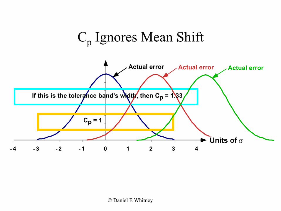
Cp Ignores Mean Shift

Actual error

Cp = 1

Actual error Actual error

If this is the tolerance band's width, then Cp = 1.33

Units of σ - 4 - 3 - 2 - 1 0 1 2 3 4

© Daniel E Whitney

Logic Tree for TolerancingHOW TO MEET

ASSEMBLY TOLERANCES

Cpk > 1: SAMPLE INSP

Cpk < 1: 100% INSP

PROBABILITY OF MEETING ASSEMBLY

TOLERANCES IS HIGH ENOUGH ­

PARTS ARE INTERCHANGEABLE

ALMOST ALL THE TIME

ERRORS GROW WITH √ N

USE SPC & Cpk ON PARTS TO KEEP PROCESS MEAN =

NOMINAL

PART TOL = ASSY TOL / √N

IF PROCESS MEAN = NOMINAL

BUILD TO PRINT

STATISTICAL TOLERANCING

STATISTICAL COORDINATION

TOOL & DIE BUILD TO PRINT

(NET BUILD)

NO COORDINATION

100% INSPECTION

PART TOL = ASSY TOL / N

ERRORS GROW WITH N

MEETS ASSEMBLY TOLERANCES

100% OF THE TIME ­PARTS ARE

INTERCHANGEABLE

WORST CASE TOLERANCING

FAILURE TO USE SPC LEADS

TO UNDOCUMENTED MEAN SHIFT

DETERMINISTIC COORDINATION

FITTING TOOL & DIE ADJUSTMENT

(FUNCTIONAL BUILD)

100% INSPECTION

BALANCE DISTRIBUTIONS

RESET NOMINAL TO PROCESS

MEAN

IGNORE MEAN, USE SPC & CP ON PARTS,

MAY BE HARD TO DIAGNOSE PROBLEMS

LATER USE SPC & Cpk ON PARTS

TOO HARD OR NOT ECONOMICAL TO MEET ASSEMBLY

TOLERANCES WITHOUT COORDINATION ­PARTS ARE NOT

INTERCHANGEABLE

SIMULTANEOUS MACHINING

SELECTIVE ASSEMBLY

LOGIC TREE OF TOLERANCING

© Daniel E Whitney