variation of greenhouse gases in urban areas-case study...

15

Variation of Greenhouse Gases in Urban Areas-Case Study: CO2, CO and CH4 in

Three Romanian Cities

Iovanca Haiduc and Mihail Simion Beldean-Galea

Babeş-Bolyai University, Faculty of Environmental Science, Cluj-Napoca,

Romania

1. Introduction

The natural equilibrium of atmospheric gases has been maintained for millions of years, but with the beginning of the industrial age, it became more fragile due to human activity. In the Intergovernmental Panel on Climate Change Report (IPCC) named “Climate Change 2007” (IPCC-AR4, 2007) it is specified that “the keep going emissions of the greenhouse gases (GHG) at/over current rate, will cause in the future global warming and will induce more global climate changes in the 21st century than those of 20th century”. More than , in the coming IPCC Report named “Carbon cycle including ocean acidification (CCT)” (IPCC-AR5, 2010) is stipulated that ocean acidification will be a further critical and direct consequence of increasing atmospheric GHG concentrations. In 1886, the chemist Svante Arrhenius (Nobel prize for Chemistry in 1903) calculated for the first time the CO2 contribution (from fossil fuel combustion) to climatic changes and used for the first time the term of “greenhouse effect”. Almost 100 years were necessary for the confirmation of Arrhenius predictions about the evolution of global climatic factors, and the fact that CO2 is the main greenhouse gas, with a contribution of 55% to Global Warming Effect. The first IPCC Report (IPCC-FAR, 1990) draws the conclusion about the possible existence of a global warming phenomenon. The second IPCC Report (IPCC-SAR, 1995) shows the contribution of humans to global warming and predicts a major warming in the 21st century. The third IPCC Report (IPCC-TAR, 2001) affirms a very probable (60% - 90%) warming for the next century. In the IPCC-AR4 Report (IPCC-AR4, 2007) adds for the understanding of the impact of climate changes over the vulnerability and the adaptation of the environment, the most relevant scientific, technical and socio-economical information from more than 1500 scientific papers. This report accepts with a probability of over 90% that the emission of greenhouse gases and not the environmental conditions gives the global warming effect. The IPCC Guide from 2006 makes an inventory of gases from atmosphere and distinguishes between: a. gases with GWP (Global Warming Potential) listed in IPCC 2001: CO2, CH4, N2O, hydro

fluorocarbons, per fluorocarbons, SF6, NF3, SF5CF3, halogenated ether, C4F9OC2H5, CHF2OCF2OC2F4OCHF2, CHF2OCF2OCHF2 and other halocarbons CF3I, CH2Br2, CHCl3, CH3Cl, CH2Cl2.

www.intechopen.com

Air Quality - Models and Applications

290

b. gases without GWP: C3F7C(O)C2F5, C7F16, C4F6, C5F8 and C4F8O. As a follow-up of these reports, the scientific community had started a cycle of research programs having as scientific goal the complex study (emission sources, consumption sources, the balance of changes between the components of environment etc.) of these gases and the effect produced by them (Projects CARBOEUROPE, AEROCARD, CHIOTTO, Global Carbon Project, IGOS, NACP etc). The CO2 it is an important green-house gas and it level in the atmosphere has significantly increased from 280 ppm in the pre-industrial era to current 380 ppm. The first increase of 50 ppm occurred during a period of ca. 200 years, starting with the beginning of the industrial revolution until 1973. Between 1973 and 2006 the concentration of CO2 increased with another 50 ppm. The Global Warming Potential (GWP) for CO2 is conventionally choose as 1, i.e. the atmospheric residence time between 50 and 200 years, and its contribution to the greenhouse effect is ca. 52 %. According to IPCC Report (IPCC-AR4, 2007), the contribution of anthropic CO2 is predominant, and the main anthropic sources are: - the energetic sector 30 % - industrial processes 20 % - fuels used in transportation 20 % - burning of biomass 9.1 % - processing and distribution of fossil fuels 8.4 % - other sources 12.5% According to IPCC estimations, the increase of CO2 concentration in the atmosphere leads to

climate changes and will produce a global warming of the planet through the greenhouse

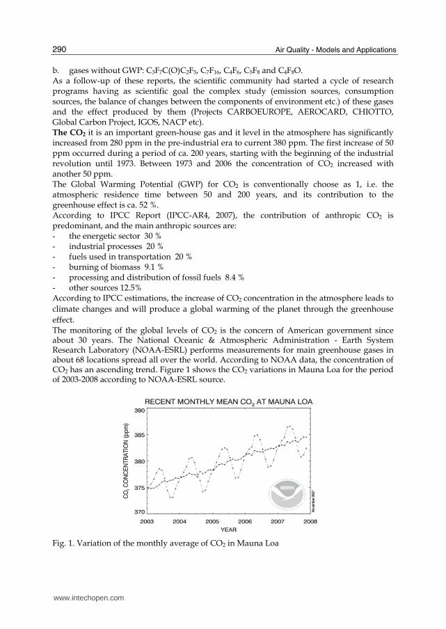
effect. The monitoring of the global levels of CO2 is the concern of American government since about 30 years. The National Oceanic & Atmospheric Administration - Earth System Research Laboratory (NOAA-ESRL) performs measurements for main greenhouse gases in about 68 locations spread all over the world. According to NOAA data, the concentration of CO2 has an ascending trend. Figure 1 shows the CO2 variations in Mauna Loa for the period of 2003-2008 according to NOAA-ESRL source.

Fig. 1. Variation of the monthly average of CO2 in Mauna Loa

www.intechopen.com

Variation of Greenhouse Gases in Urban Areas- Case Study: CO2, CO and CH4 in Three Romanian Cities

291

At the European level, the Carboeurope-Clusters Program (CarboEurope) carries out measurements of atmospheric CO2 concentrations in 61 locations in 17 countries. This program contains eight different projects working together to contribute to the understanding of the carbon cycle at the European level. The projects involved in this program are: AEROCARB, CAMELS, CARBOAGE, CARBODATA, CARBOEUROFLUX, CARBOEUROPE GHG; CARBOINVENT, CHIOTTO, CARBODATA, TACOS, EUROSIBERIAN CARBONFLUX, FORCAST, GREENGRASS, RECAB, TACOS-INFRASTRUCTURE, and TCOS SIBERIA. Two other projects, CARBOMONT and SILVISTRAT are associated to this program. In 1998 Idso and co-workers (Idso et al., 2001) introduced the term ““urban DOME” for the persistence of CO2 over the urban cities as a result of anthropogenic contribution to CO2 budget. After that, several individual studies regarding to CO2 variation in urban areas have been reported (Day et al., 2002; Idso et al., 2002). These studies showed that the concentration of CO2 in urban area is higher that the CO2 concentration in rural area and this fact is a consequence of human activities. A literature review about these results is presented in this chapter. Methane (CH4) is another important greenhouse gas, with GWP = 25 and a residence time of more than 100 years. It is produced both naturally and through human activities. The global mixing ratios of CH4 in the atmosphere have more than doubled since the pre-industrial period, rising from around 750 ppb (parts per billion) in 1800 (Simpson et al., 2002; Dlugokencky et al., 2003) to the current level of around 1770 ppb (NOAA-ESRL). The global trend of the methane concentration in the air is ascending, with a rate of increase of 5–10 ppb/year, and for the period 1984-2004 this tendency is shown in Figure 2.

Fig. 2. The variation of the global average concentration of CH4. (source NOAA-ESRL)

The main natural source of methane are dominated by wetlands. The primary way for CH4

transformation is its destruction in the atmosphere by hydroxyl radicals (Prinn et al., 1995,

2001). Some CH4 is also oxidized by microorganisms (called methanotrophs), which use CH4

as a source of carbon and energy. Tropospheric CH4 is eventually oxidized to carbon

dioxide; its atmospheric lifetime is estimated to be 8–12 years (NOAA-ESRL; Cunnold et al.,

2002; IPCC-AR4, 2007).

It is estimated that the contribution of methane to the greenhouse effect is 18%, and the most

important sources are:

- Residual agricultural products 40% - Processing and distribution of fossil fuels 29.6%

www.intechopen.com


292

- Storage and processing of domestic waste 18.1%

- Burning of biomass and grazing 6.6%

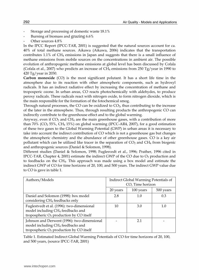
- Other sources 4.8% In the IPCC Report (IPCC-TAR, 2001) is suggested that the natural sources account for ca. 40% of total methane sources. Aikawa (Aikawa, 2006) indicates that the transportation contributes 1.1% of CH4 emissions in Japan and suggests that there is a small influence of methane emissions from mobile sources on the concentrations in ambient air. The possible evolution of anthropogenic methane emissions at global level has been discussed by Cofala (Cofala et al., 2007) who predicts an increase of CH4 emissions from 250 Tg/year in 1990 to 420 Tg/year in 2030. Carbon monoxide (CO) is the most significant polutant. It has a short life time in the atmosphere due to its reaction with other atmospheric components, such as hydroxyl radicals. It has an indirect radiative effect by increasing the concentration of methane and troposperic ozone. In urban areas, CO reacts photochemically with aldehydes, to produce peroxy radicals. These radicals react with nitrogen oxide, to form nitrogen dioxide, which is the main responsible for the formation of the fotochemical smog. Through natural processes, the CO can be oxidized to CO2, thus contributing to the increase of the later in the atmosphere. Thus, through resulting products the anthropogenic CO can indirectly contribute to the greenhouse effect and to the global warming. Anyway, even if CO2 and CH4 are the main greenhouse gases, with a contribution of more than 70% (CO2 55%, CH4 15%) on global warming (IPCC-AR4, 2007), for a good estimation of these two gases to the Global Warming Potential (GWP) in urban areas it is necessary to take into account the indirect contribution of CO which is not a greenhouse gas but changes the atmospheric chemistry and the abundance of other greenhouse gases. CO is a key air pollutant which can be utilized like tracer in the separation of CO2 and CH4 from biogenic and anthropogenic sources (Daniel & Solomon, 1998). Different studies (Daniel & Solomon, 1998; Fuglesvedt et al., 1996; Prather, 1996 cited in IPCC-TAR, Chapter 4, 2001) estimate the indirect GWP of the CO due to O3 production and to feedbacks on the CH4. This approach was made using a box model and estimate the indirect GWP of CO for time horizons of 20, 100, and 500 years. The indirect GWP value due to CO is gave in table 1.

Authors/Models Indirect Global Warming Potentials of CO, Time horizon

20 years 100 years 500 years

Daniel and Solomon (1998): box model considering CH4 feedbacks only

2.8 1.0 0.3

Fuglestvedt et al. (1996): two-dimensional model including CH4 feedbacks and tropospheric O3 production by CO itself

10 3.0 1.0

Johnson and Derwent (1996): two-dimensional model including CH4 feedbacks and tropospheric O3 production by CO itself

- 2.1 -

Table 1. Estimated Indirect Global Warming Potentials of CO for time horizons of 20, 100, and 500 years, (source IPCC-TAR, 2001)

www.intechopen.com


293

Regarding to long time measurement of CO2 concentration in urban area as well as the variation of meteorological parameters allow to understanding the rule of the ecosystem functioning and meteorological parameters over inter-annual variation in carbon fluxes. The inter-annual variation of CO2 fluxes has been typically studied either by modeling approaches (Higuchi et al., 2005; Ito et al., 2005; Bergeron & Strachan, 2011) or by correlation coefficient analyses together with meteorological parameters (Aubinet et al., 2002; Aurela et al., 2004; Wohlfahrt et al., 2008). These studies showed that, the CO2 flux is strongly influenced by biological vegetation cycle and the variation of meteorological parameters. Thus the maximum value of CO2 is registered during the cold season while the minimum value of CO2 was registered during the summer. Another study (Sottocornola & Kiely, 2010), show that the wet conditions favored the CO2 uptake by the ecosystem in autumn and in winter, while the warmer and dryer weather reduce the sequestration of CO2 in the ecosystem. A study performed in urban and sub-urban area of Montreal (Bergeron & Strachan, 2011) showed that the CO2 flux is also influenced by the anthropic activity. According to this study, “Lower emissions at the suburban site are attributed to the large biological uptake in summer and to its relatively low population density inducing low anthropogenic emissions. Higher emissions at the urban site are partly associated with its greater population and building density, promoting higher emissions from vehicular traffic and heating fuel combustion. Vehicular traffic CO2 emissions influenced the diurnal cycle of CO2 fluxes throughout the year at the urban site. At the suburban site, summer CO2 fluxes were dominated by vegetation sources and sinks as daytime CO2 uptake occurred and CO2 fluxes responded to incoming light levels and air temperature in a fashion similar to natural ecosystems. To a lesser extent, the vegetation component also helped offset CO2 emissions from other sources in summer at the urban site.” This chapter will present the results of a case study of CO2, CH4 and CO variations during one year in three selected cities from Romania with different anthropic activity. In order to identify the influence of biogenic and anthropogenic sources to the budget of mentioned greenhouse gases the 13CO2 and 13CH4 isotopic composition have been determinate. Experimental results were finally correlated with meteorological parameters.

2. CO2 in urban area

2.1 Trends of CO2 variation in urban areas. A literature review

The problem of urban carbon dioxide came into the attention of scientists in the year 1998, with the discovery and characterization of the urban CO2 dome of Phoenix, Arizona, USA by Idso and col. (Idso et al., 2001). Early work found that under certain meteorological conditions, urban CO2 concentrations could be as high as 550-600 ppm (some 200 ppm higher than the surrounding countryside) (Idso et al., 2002). Soegaard and Moller-Jensen (Soegaard & Moller-Jensen, 2003) studied the urban CO2 dome of Copenhagen and indicated that "traffic is the largest single CO2 source in the city," and demonstrate that "emission rates range from less than 0.8 g CO2 m-2 h-1 in the residential areas up to a maximum of 16 g CO2 m-2 h-1 along the major entrance roads in the city center." Following these studies, research regarding the urban CO2 domes has been performed in

many other parts of the world (Table 2). The results obtained from studies conducted in

several cities from all over the world, show several commonalities. Thus, anthropogenic CO2

emissions are the primary source of the urban CO2 dome; the dome is generally stronger in

city centers, in winter, on weekdays, at night, under conditions of heavy traffic, close to the

ground, with little to no wind, and in the presence of strong temperature inversions. These

www.intechopen.com


294

conclusions are in agreement with the data provided by Commonwealth Scientific and

Industrial Research Organisation (CSIRO) which indicate that typical concentrations of CO2

in urban areas is situated between 350 and 600 ppm and depend on meteorological

parameters and urban agglomeration.

Authors Place of measurements

Period of measurement

CO2 range concentrations

Coutts A. M. Melbourne, Australia

February -July, 2004

355 - 380 ppm (daily mean concentration).

Day T. A. et al.

Phoenix, USA March -April, 2000

377 - 396 ppm (daily mean concentration)

George K. et al.

Baltimore, USA 2007 488 in urban area, 442 in sub-urban area, 422 in rural area

Ghauri B. Six cities, Pakistan

2003 - 2004

270 - 325 ppm in Islamabad, 289 - 389 ppm in Quetta, 316.5 - 360 ppm in Karachi, 324.1 - 380 ppm in Lahore 295.2 - 356 ppm in Rawalpindi, 312 - 382 ppm in Peshawar.

Gratani L. et al.

Rome, Italy 1995 - 2004

367 ± 29 ppm in 1995 (montly mean variation) 477 ± 30 ppm in 2004 (montly mean variation) 414 ± 25 ppm green zone 505 ± 28 centrale zone

Grimmond et al.

Chicago, USA July 11-August 14, 1995

338 - 370 ppm (diurnal variation) 405 - 441 ppm (nightly variation)

Idso S. B. et al.

Phoenix, USA 2000

390.2 ± 0.2 ppm (minimum daily concentration) 424.3 - 490.6 ppm (maximum daily concentration) 619.3 ppm (maximum daily concentration in cold season)

Kuc T. et al. Kasprowy Wierch and Krakow, Poland

2000

370 ppm (monthly mean variation in Kasprowy Wierch) 370 - 430 ppm (monthly mean variation in Krakow)

Moriwaki R. et al.

Tokyo, Japan October-Nov., 2005

380 - 580 ppm (daily mean concentration).

Nasrallah H.A. et al.

Kuwait City, Kuwait

1996 - 2001 368 - 371 ppm (daily mean concentration at 7 metter high).

Velasco E. et al.

Mexico city, USA

June 11-August 14, 1995

398 – 444 ppm (daily variation) 421 ppm (daily mean)

Table 2. Overview of urban CO2 measurements

Taking in to account the concentration of CO2 from the cities, some of researches were focused on the impact of local CO2 emissions over local temperature. Thus, Balling et al. running the CO2 concentration though a radiation model calculated that local CO2 emissions modify the local temperature with more than one-tenth of one degree Celsius. In fact, Balling

www.intechopen.com


295

et al. sugest that this increasing of temperature is insignificant by comparing it to the overall urban heat island in Phoenix which typically adds 5 to 10 degrees C. (Balling, Jr., et al., 2001). Recently, Jacobson (Jacobson, 2010) found that domes form above cities more than a decade ago, cause local temperature increases that in turn increase the amounts of local air pollutants, raising concentrations of health-damaging ground-level ozone, as well as particles in urban air. Also, this study has shown that “CO2 dome” that develops over urban areas is a local problem, which creates much more health problems than in rural areas. The conclusions of Jacobson about the human health effects of CO2 created many controversies; therefore, more research is necessary on the measurement of CO2 variation over the urban areas.

2.2 CO2 variation in three Romanian cities. Case study

The available literature contains no information about the variation of CO2 concentrations in Romania in urban areas. However, the American system of global monitoring of CO2 (NOAA-ESRL) has a station of continuous measurement of the main parameters of air quality placed in Constanta, which also measures CO2 concentrations. According to NOAA-ESRL data, the variation of CO2 concentrations at the Constanţa measurement station has an ascending trend; the yearly average values are between 365 ppm in 1995 and 395 ppm in 2007. According to the same source the concentration of CO2 has a seasonal variation with maxima in the cold season and minima in the warm season. In order to study the influence of anthropic activity upon the CO2 level the study was performed in three different Romanian cities from Cluj County, as follows: a. Cluj-Napoca city, 400 000 inhabitants, b. Turda city, 59 600 inhabitants c. Huedin town, 10 000 inhabitants The case study has been carried out during one year (four seasons) from July 2008 to June 2009. The measurements were performed monthly (during 8 hours from 8.30 am to 15.30 pm) in all the three selected locations using a NDIR CO2 analyzer model EMG-4. The measurements of CO2 levels were performed in a portable meteorological shelter. For the estimation of the anthropogenic contribution over the CO2 budget in all three studied areas a reference point situated outside of the cities has been chosen (Roba et all, 2009). For the Cluj-Napoca city,three measurement points have been selected: one situated in a zone

with intense traffic (Piaţa Mărăşti), one with moderate traffic (Cartier Grigorescu) and a

reference point located in a periphery location (meteorological station in Cartier Gruia).

The results of the measurements recorded in the three locations in the city of Cluj-Napoca

show that during the year the CO2 level is strongly influenced by the amplitude of the

anthropic activities. The highest levels were recorded in the location with intense anthropic

activity (Piata Marasti) and the lowest levels in the reference point located outside of the

city. The recorded values are comprised between 380 and 530 ppm (Mărăşti), 376-456

(Grigorescu) and 373-444 (reference point).

It was also found that the highest values were recorded during the months of October and

November (during the final period of the biological cycle of plants) and during the winter. It

was also found that starting with the months of March; the CO2 concentrations decrease and

become comparable with the summer values (Figure 3).

www.intechopen.com


296

For the Turda city two measurement points have been selected: one in the city (Potaisa

School) and another one located outside of the city (Meteo Station).

The results of the measurements in the two locations indicate a concentration difference

between 15 and 20 ppm, depending of the period of measurements. The largest values of

CO2 concentration were obtained in the months of October and November, at the end of the

biological cycle of plants and in the winter. The concentrations measured are in the range

380-502 ppm at Potaisa site and 371-450 ppm at the reference point.

In the town of Huedin the measurements were carried out simultaneously in two locations:

one in the interior of the city (Liceul Octavian Goga) and a reference point in the peripheral

area (Meteo Station). The results show a slight difference between the two locations. It was

also observed again that the largest values are recorded in the months of October and

November, i.e. at the end of the biological cycle of plants, and during the winter.

Starting with the month of March, the CO2 concentrations decrease to normal values,

comparable to those of the summer. The values recorded are in the range 355- 433 ppm

(Octavian Goga site) and 350-411 ppm (reference point).

A comparison of the measured values carried out in different locations shows that the CO2

concentrations depend on the size of the town, the highest values being recorded in Cluj-

Napoca city, followed by Turda and Huedin (Figure 3).

CO2, Cluj-Napoca City

30

03

50

40

04

50

50

05

50

July

August

Septem

ber

Octo

ber

November

December

January

February

Marc

hApril

May

June

CO

2 [

pp

m]

Marasti

Grigorescu

Reference Point

CO2, Turda

350

370

390

410

430

450

470

490

510

530

550

July

August

Septem

ber

Octo

ber

November

December

January

February

Marc

hApril

May

June

CO

2 [

pp

m]

Potaisa

Reference Point

CO2, Huedin

350

400

450

500

550

July

August

Septem

ber

October

November

December

January

February

Marc

hApril

May

June

CO

2 [

pp

m]

O.Goga

Reference Point

CO2, Cluj - County

350

400

450

500

550

July

August

Septem

ber

October

November

December

January

February

Marc

hApril

May

June

CO

2 [

pp

m]

Cluj-N

Turda

Huedin

Fig. 3. Annual variation of CO2 in urban studied areas

www.intechopen.com


297

Diurnal variations were also observed; the highest values were measured in the morning and the lowest values at the astronomic midday, both in summer and in winter seasons (Figure 4).

Diurnal CO2 variation - September

350

370

390

410

430

450

470

490

8:30

9:30

10:30

11:30

12:3

0

13:3

0

14:30

15:30

ora

CO

2 [

pp

m]

Cluj-Napoca

Turda

Huedin

Diurnal CO2 variation - January

350

370

390

410

430

450

470

490

510

530

8:30

9:30

10:3

0

11:3

0

12:3

0

13:3

0

14:3

0

15:3

0

ora

CO

2 [

pp

m]

Turda

Cluj-Napoca

Huedin

Fig. 4. Diurnal variation of CO2 in urban studied areas

Taking into account the results of this case study we can conclude that the variation of CO2 in studied urban areas is in agreement with other results reported in the scientific literature, which report that in urban areas the CO2 levels are situated between 350 and 600 ppm, depending on meteorological parameters and urban agglomeration, with the observation that in the absence of rainfall the CO2 level increases both in urban areas and outside.

3. CH4 in urban area

3.1 Trends of CH4 variation in urban areas. A literature review

Regarding to CH4 variation in urban areas there are only a few studies about the level of methane in urban atmosphere, and these results are reported starting after the year 1980. For Romania such data are available only after 1995. According to data from CSIRO the common concentrations of CH4 in urban areas have values between 1700-2500 ppb and are influenced by meteorological parameters and urban agglomeration. Kuc and co-workers (Kuc et al., 2003) show that, the CH4 level in urban areas is comprised between the natural level (1650 ppb) and 4200 ppb. Ito and co-workers (Ito et al. 2000) compared the atmospheric CH4 concentrations recorded in Nagoya with the values measured at Mauna Loa Observatory in Hawaii (USA) and estimated that the excess concentration of CH4 in the urban atmosphere of Nagoya was 170 ppb in 1988 and 150 ppb in 1997. A selective bibliography on the subject in presented in Table 3.

3.2 CH4 variation in three Romanian cities. Case study

In Romania, the available literature provides no information about the variation of methane concentrations in urban areas and no such studies are reported. However, the American System of Global Monitoring of Air Quality (NOAA-ESRL), has a station of continuous measurements of atmospheric methane concentrations at Constanţa. According to NOAA data, the concentration of CH4 has an ascending trend, with average values comprised between 1880 ppb in 1995 and 1980 ppb in 2006. According to the same source, the methane concentration shows a seasonal variation, with maxima in the summer months and minima in the autumn and spring.

www.intechopen.com


298

Authors Place of measurements

Period of measurement

CH4 range concentrations

Aikawa M. et al.

Urban,Sub-urban, Nagoya, Japan

2004 1.80 - 1.84ppm -urban area 1.78 - 1.80 ppm-suburban area

Derwent R.G. et al.

Island 1990 - 2003 1.75 - 2.00 ppm

Ghauri B. et al.

Pakistan 2003 - 2004 0.5 – 1.7 ppm

Hsu Y.K. et al. California, USA

April 2007 - Feb. 2008

1.75 - 2.16 ppm

Ito A. et al. Nagoya, Japan 1983 – 1997 1.85 ppm in 1998, 1.91 ppm in 1995, 1.90 ppm in 1997. 1983 - 1997 increese 13 ppb/year

Kuc T. et al Kasprowy Wierch Krakow, Poland

2000 1650 ppb Kasprowy Wierch (monthly mean concentration) 2000 - 2800 ppb Krakow (monthly mean concentration)

Sikar E. & La Scala N.

Urban area, Brasil

1998 – 1999 1.80 ppm

Smith F.A. et al.

Mexico City March, 1993 1.8 ppm during the night 7.971 ppm in the morning 2.001 - 2.999 midle of the day

Thi Nguyen H et al.

Seul, Korea 1996 - 2006 2.24 ± 0.42 ppm urban road-side 2.06 ± 0.31 ppm urban background

Veenhuysen D. et al

Amsterdam, Netherlands

1994 1.75 - 3.00 ppm

Wang J.L. et al.

Sub-urban area, Taiwan

1-27 April, 2000

1.9 - 3.7 ppm

Table 3. Overview of urban CH4 measurements

Our case study has been focused on the measurement of the CH4 variation in three urban areas from Cluj county as described in sub-chapter 2. The study was carried out during one year (four seasons) from July 2008 to June 2009. The measurements were performed monthly in all selected areas at the astronomic midday (in Romania at 12.30 h). In all three areas a measurement point located in the city and a reference point located outside has been selected. The samples were collected in Cluj-Napoca, in Marasti location in the city and as reference

point at Gruia location. In Turda the measurements in the city were made at Liceul Potaisa,

and the reference point at the Meteo station. In Huedin the measurements were made at

Liceul Octavian Goga in the town and the reference point was the meteo station.

For atmospheric CH4 measurements, the air samples where collected by the flask sampling

method and analysed by gas chromatography technique (GC) coupled with a flame

ionisation detector (FID) (Cristea et all., 2009).

The results show a signficant variation of atmospheric methane, depending on the season

and the urban aglomeration degree. Thus, the highest values were recorded in the city of

Cluj-Napoca (11.5 ppm in April 2009) and the lowest values were recorded in the month of

August 2008 (2.5 ppm).

www.intechopen.com


299

In Turda the concentrations of atmospheric methane were comprised between 2.2 and 8.6 ppm, with the lowest values measured in August 2008 (2.2 ppm) and the highest values recorded in April 2009 (8.6 ppm). In Huedin the concentrations of methane were measured between 1.4 and 7 ppm, with the lowest values recorded in July 2008 (1.4 ppm) and the highest ones in April 2009 (7 ppm). Significant differences are also bserved between te methane concentrations in the interior of the cities and the reference points located outside. These differences were recorded throughout the experiments, which leads to the conclusion that the anthropic activities, the automobil traffic in particular, are an important source of methane in the urban atmosphere. The analysis of the methane concentrations in the three areas investigated indicates a similar profile for the measurements in the interior of the cities, with minima in the summer months and maxima during the spring. This may be attributed to the absence of rains in the spring (March-April). In May 2009, when the precipitations started, the concentration of atmospheric methane became closer to the values measured at the reference points. For the reference points, the values of the atmospheric methane concentrations are in the range 2.1-4.2 ppm in Cluj-Napoca, 1.7-3.5 in Turda and 1.4-2.9 ppm in Huedin. As for the measurements in the city, a slight increase of the concentrations were observed in the spring period of 2009, due to the lack of precipitations.

CH4, Cluj-Napoca City

0

2

4

6

8

10

12

14

July

August

Septem

ber

Octo

ber

November

January

February

Marc

hApril

May

June

CH

4 [

pp

m]

Marasti

Reference Point

CH4, Turda

0

2

4

6

8

10

12

14

July

August

Septem

ber

Octo

ber

November

January

February

Marc

hApril

May

June

CH

4 [

pp

m]

Potaisa

Reference point

CH4, Huedin

0

2

4

6

8

10

12

14

July

August

Septe

mber

Octo

ber

November

January

Februar

y

Marc

hApril

May

June

CH

4 [

pp

m]

O. Goga

Reference Point

CH4, urban areas - Cluj County

0

2

4

6

8

10

12

14

July

August

Septem

ber

Octo

ber

November

January

February

Marc

hApril

May

June

CH

4 [

pp

m]

Cluj-Napoca

Turda

Huedin

Fig. 5. The variation of methane concentration in the urban areas of Cluj county locations.

www.intechopen.com


300

The results of our measurements indicate that the atmospheric CH4 level in urban areas is strongly influenced by the size of the urban aglomeration as well as by the meteorological parameters. These results is in agreement with other results from scientific literatures.

4. CO in urban areas

4.1 Trends of CO variation in urban areas. A literature review

According to World Health Organization data (WHO, 2000), in the main European cities the average atmospheric CO concentration is situated under 2 mg/m3 air, with a maximum concentration lower than 6.0 mg/m3 air. At global level, the concentration of CO is composed between 0.05 and 0.12 ppm in the air. This concentration is an average between the values measured in urban and rural areas. In rural areas the CO concentration is due mainly to natural processes, but in urban areas it is strongly influenced by anthropic activities. The CO concentration in the air of urban zones depends upon the density of combustion sources, the topography of the measurements location, the meteorological conditions and from the distance between the measurement point and the auto traffic routes. The monitoring of CO in USA is carried out since 1980; currently, there are 243

measurement stations distributed all over the USA territory. According to EPA Reports

(EPA, 2009), the concentration of CO decreased in the period 1980-2006 from 14 ppm to 3

ppm.

In Europe, the monitoring of CO in urban areas is 20 years old. Several European projects were in action, to evaluate the exposure of the population to CO, and the measurements were carried out both with fixed and mobile stations. According to WHO data (WHO, 2000) in large European cities the CO concentrations (during 8 hours measurements) are situated bellow 20 mg/m3 in the air, and the maxima are not higher than 10 mg/m3 in the air. The first network for the measurement of pollutants resulted from anthropic activities was created in France in 1979 under the name AIRPARIF and measures the daily, monthly and annual concentrations of NOx, SO2, O3, PM, CO and of some organic compounds. According to this source, the CO concentration in the Paris region decreased from 4000 μg/m3 air in 1994 to 1200 μg/m3 air in 2006. In 2004 started measuring background measurements. The variation of annual average decreased from 500 de μg/m3 air in 2003 to 400 μg/m3 air in 2006. In Great Britain, the measurement of the concentrations of atmospheric pollutants dates

from 1973; currently, there are more than 100 station in urban zones for continuous

monitoring of the air quality parameters. In London, the quality of air is monitorised by as

many as 30 stations. The network was created in 1993 under the name London Air Quality

Network (LAQN), and since 1997 this network also measures the evolution of daily CO

concentrations.

At the European level functions the European Environment Agency (EEA) with 32

members: all the 27 EU member countries, also Island, Liechtenstein, Norway, Switzerland

and Turkey. Under the coordination of EEA was created the European Environment

Information and Observation Network (EIONET), with the role of processing and validating

the data from the stations of the member countries connected to this network. The

information is available as Reports to interested users. Among the workstations connected

to EIONET, 163 measure the concentrations of CO. According to EEA data, the

concentration of CO at the European level decreased from 1 mg/m3 air in 1995 to 0.5 mg/m3

air in 2005.

www.intechopen.com


301

In addition to the data from the monitoring stations there are numerous studies about the

determination of CO concentrations in urban zones all over the world. A synthesis of these

results is given in Table 4.

Authors Place of

measurements Period

measurement CO range concentrations

[ppm]

Chatterton T.et al. Norwich, UK 1997 - 1998 0.4 - 10.9

Chelani A.B. et al. Delhi, India 2000 - 2003 1.66 - 8.4

Cheng C. S. et al. Canada 1974 - 2000 Montreal: 0.5 - 2.1, Toronto: 0.7 - 3.7

Corti A. et al. Salerno, Italy Not specified 0.55 - 0.85

DEQ-Oregon Portland-SUA 1980 - 1998 13.0 - 4.7

Emmerson K. et al. Birmingham, UK 1999 - 2000 0.17 - 0.66

EPA USA 1990 - 2006 Washington (decrease from 9 to 2), New-York (8.6 - 1.8), Los Angeles (14 – 4) ,

Ghauri B. et al. Pakistan 2003 - 2004 Islamabad : 6 - 13; Quetta: 1.9 - 14 , Karachi: 1.6 - 8.0; Lahore: 1.3 - 12; Rawalpindi: 1.6 - 8

Ghose M. K. et al. Calcutta, India 2003 2.6 - 5.1

Jones S. G. et al. Paris, France 1997 0.38 - 1.45

Kim S.Y. et al. Seoul , Koreea 2002 0.8 - 44.0

Kukkonen J. et al. Helsinki, Sweden 1997 0.1 - 4.5

Lijteroff R. et al. San Luis, Argentina

1994 - 1995 3.43 - 9.17

Linden J. et al. Burkina Faso, Africa

2004 - 2005 Background: 1 - 9, Traffic: 6.5 - 6.0

Makra L. et al. Szeged, Hungary 1997 - 2001 0.24 - 0.93

Manning A.J. et al. Leek, UK 1997 0.25 - 4.0

Martín M.L. et al. Bay of Algeciras 1999 - 2001 0.5 - 2.9

Milton R. et al. Londra, UK 2004 - 2005 0.9 - 14.9

Muttamara S. et al. Bangkok 1997 8.23 - 26.89

Ni-Bin Chang et al. Kaohsiung, Taiwan

1995 0.1 - 2.0

Park S. S. et al. Seoul, Koreea 1998 - 1999 1.74 - 2.81

Reich S. et al. Buenos Aires 2001 0.60 - 2.44

Rubio M. A. et al. Santiago City, Chile

2005 - 2006 0.31 - 3.06

Sanchez-Coyllo O. et al.

Sao-Paulo, Brazilia 1999 1.20 - 4.00

Sathitkunarat S. et al.

Chiang Mai, China 2002 0.9 - 1.5

Shiva Nagendra S.M.

Delhi, India 1997 - 1999 0.1 - 18

Turias I.J. et al. Campo de Gibraltar

1999 - 2001 0.4 - 4.5

Venegas L.E. et al. Buenos Aires 1994 - 1996 Autumn:10,0, Winter: 9.80, Spring :10,7

Table 4. Overview of urban CO measurements

www.intechopen.com


302

4.2 Case study Cluj-Napoca city

In Romania, the monitoring of air quality is done by the Agencies for Environment Protection and follows the concentrations of nitrogen oxides, sulfur dioxide, ozone, BTEX, material particles, etc. Of these, 53 monitoring stations are connected to the European EIONET System and 12 stations also measure the concentrations of CO in urban zones. In the city of Cluj-Napoca, there are four stations for continuous monitoring of air quality, and beginning with August 2005 the Agency measures the CO concentrations in two locations in the city of Cluj-Napoca and one in the city of Dej. The measurements in Cluj county show that the concentration of CO in the atmosphere is much below the admitted level (10 mg/m3) and varies between 0.09 and 0.4 mg/m3 air. In this case study the measurements were performed daily in Cluj-Napoca at the astronomic midday (in Romania at 12.30 h) using a NDIR CO analyzer Horiba model APMA-360. The results showed that the CO level in Cluj-Napoca is less than 1 mg/m3 with a tendency of accumulation during the winter season. It is also observed a trend of accumulation during the spring months, due to the lack of precipitations. Beginning with the end of May, when the rain regime becomes normal, the values of CO concentrations are around 0.1 mg/m3 air (Figure 6).

0

0.1

0.2

0.3

0.4

0.5

0.6

0.7

0.8

0.9

1

1 iulie

23 iu

lie

11-A

ug

27-A

ug

11 sep

t.

29 sep

t.

13 o

ct.

30 o

ct.

17 n

ov.

1 de

c.

07.0

1.09

26.0

1.09

09.0

2.09

27.0

2.09

16.0

3.09

03.0

4.09

21.0

4.09

13.0

5.09

04.0

6.09

20.0

6.09

CO

(m

g/m

3 a

er)

CO

Fig. 6. Variation of CO concentrations in Cluj-Napoca in the period July 2008-June 2009

5. Anthropogenic contribution in CO2 and CH4 budgets

5.1 Isotopic 13

CO2 measurements

Knowledge of the terrestrial CO2 cycle will help to understand the climate change

phenomena and to predicting the future atmospheric CO2 concentrations and global

temperatures. By estimating the terrestrial CO2 cycle, including such factors as emissions,

storages and fluxes and combining this with the isotope compositions of atmospheric CO2

will help to identify the contribution of different factors to the atmospheric CO2 budget.

More than the observation of the CO2 isotopic composition provides important information

about sources such as fossil fuel combustion and biogenic respiration. The determination of

isotopic concentrations of 13C enforces the analyze of different species of atmospheric CO2

and CH4 collected in situ in glass recipients of different measures (flask sampling) by mass

spectrometry. Thus, Takahashi et al. (2001, 2002) using CO2 isotope compositions method

www.intechopen.com


303

for investigating the sources of atmospheric CO2 observed carbon isotope compositions of

Δ14C and ├13C in atmospheric CO2 and estimated the contributions of fossil fuels and biogenic

respiration, while Pataki (Pataki et al., 2003, 2006a,b) observing ├13C and ├18O isotope

compositions in atmospheric CO2 has reported the contribution of natural gas combustion,

gasoline combustion and biogenic respiration over the total atmospheric CO2 budget.

To identify sources of carbon and to quantify these sources it is used the Keeling plot (Pataki et al., 2003). The equation used in the Keeling plot is derived from the basic assumption that

the atmospheric concentration of a substance (CO2, CH4) in air reflects the combination of

some background amount of the substance that is already present in the atmosphere and

some amount of substance that is added or removed by sources or sinks:

CT=CA+CS (1)

where CT, CA, and CS are the concentrations of the substance in air, in the background of

atmosphere, and that contributed by sources, respectively. Isotope ratios of these different

components can be expressed by a simple mass balance equation:

CT├T=CA├A+CS├S (2)

where ├T, ├A, and ├S represent the isotopic composition of the substance in the atmosphere, in the background, and of the sources, respectively. By combine Eqs. 1 and 2 it is obtained equation 3:

├T = CA (├A –├S)(1/ CT)+├S (3)

This is a linear relationship with a slope of CA (├A –├S) and an intercept at the ├S value of the net sources/sinks in the atmosphere. According to Pataki (Pataki et al., 2006) the mixing ratios originating from local sources (CS) is composed from the CO2 mixing of natural gas combustion (CN) and CO2 mixing of gasoline combustion (CG):

CT = CA + CN + CG (4)

Using the values of measured concentrations of CO2 (CT) in the same time and in the same air as the measurements of ├T, and know the ├N, ├G and CN it is possible to estimate CG. The isotopic mass balance equation in this case is:

├TCT = ├BCB + ├NCN + ├GCG (5)

where ├T and ├G represent the isotopic composition of the CO2 results from natural gas combustion and ├G is the isotopic composition of the CO2 results from gasoline combustion. In order to study the effects of the emission and diffusion of CO2 from fossil fuel combustion most of the recent studies have focused on urban areas where CO2 is mainly the product of power plants and transportation. The results of these measurements were correlated with variations in carbon isotopic composition and its show that while the natural level of ├13C value is −8.02‰, in urban areas the ├13C values is down to −12‰ for atmospheric CO2. This difference is given by the increasing input of CO2 derived from fossil fuel (Clark- Thorne and Yapp, 2003, Lichtfouse et al., 2003; Widory and Javoy, 2003, Newman S et al. 2008, Wada et al 2010).

www.intechopen.com


304

5.2 Isotopic 13

CH4 measurements

The carbon isotopic composition (12C, 13C and 14C) of atmospheric methane is used to estimate the local CH4 sources contribution over the CH4 budget in a local areas (Moriizumi et al., 1998) According to (Miller et al., 2003 cited by Cuna et al. 2008) the methane mixing ratio in air, [CH4], and its isotopic ratio, ├13CCH4, may be derived from three main sources: methane produced by microbial, [CH4]micr, fossil methane, [CH4]ff, and methane produced from biomass burning, [CH4]bmb

[CH4]T = [CH4]micr, + [CH4]ff, + [CH4]bmb+ [CH4]bg (1)

In equation (1) [CH4]bg is defined as the smoothed marine boundary layer (MBL) at the latitude of interest (Dlugokencky et al., 1994 cited by Cuna et al. 2008). Each of these emissions has a more-or-less distinct isotopic signature with bacterial methane ├13Cmicr≈ 60‰, thermogenic methane ├13Cff ≈ 40‰, and biomass burning methane ├13Cbmb≈ 25‰ (Quay et al., 1999 cited by Cuna et al. 2008).

├13C[CH4]T = ├13C[CH4]micr, + ├13C[CH4]ff, + ├13C[CH4]bmb+ ├13C[CH4]bg (2)

Separating CH4 sources using isotopic signatures is complicated by enrichment during uptake processes such as bacterial CH4 oxidation, or methanotrophy (Chanton et al., 2005 cited by Cuna et al. 2008). Thus, the methane mixing ratio changes over time according to Eq. (3), where [CH4]S is the sum of all sources and τ is the lifetime of methane with respect to its destruction by OH and addition from other processes (Montzka et al., 2000; Hein et al., 1997 cited by Cuna et al. 2008):

d[CH4] / dt = [CH4]S –([CH4]/ τ) (3)

The ├13C of methane measured in an air sample results from several different sources, such that

├13CS = ├13Cbg + ┝ (4)

In Eq. (4) ├13CS is the flux-weighted isotopic ratio of all sources expressed in ├ notation, ├13Cbg is the atmospheric background isotopic ratio and ┝ is the average isotopic fractionation associated with these processes (Cantrell et al., 1990 cited by Cuna et al. 2008 ). Using the values of measured concentrations of methane [CH4]T in the same time and in the same air as the measurements of ├13, it is possible to estimate the contribution of all sources at the atmospheric methane budget. Thus, Moriizumi (Moriizumi et al., 1998) analyzing the CH4 in Nagoya, Japan found that “the contribution of fossil CH4 to local CH4 released from the urban area was calculated to be 102±8%, and its δ13C was −40.8±3.0‰. In a suburban area of Nagoya fossil, CH4 contributed to less than 10% of local release and the calculated value of δ13C for non-fossil CH4 was approximately −65‰, which is within the range of reported values of δ13C for CH4 derived from bacterial CH4 sources such as irrigated rice paddies”. Kuc (Kuc et al. 2003), measuring the CH4 in Krakow found that “The linear regression of δ13C values of methane plotted versus reciprocal concentration yields the average δ13C signature of the local source of methane as being equal to −54.2‰. This value agrees very well with the measured isotope signature of natural gas being used in Krakow (−54.4±0.6‰) and points to leakages in the distribution network of this gas as the main anthropogenic source of CH4 in the local atmosphere”. Nakagawa (Nakagawa et al., 2005), using the stable carbon and hydrogen isotopic compositions (δ13C

www.intechopen.com


305

and δD) of methane quantified the contribution of automobile exhaust to local CH4 budget. The authors estimated that for local sources, automobile exhaust in Nagoya, Japan, contribute significant amounts (up to 30%) of CH4 to the troposphere in the studied area.

Studies performed in wetlands showed that the isotopic signature ├13C of methane is situated between -67.4 and -53.3‰ with lower values in the summer and higher values in the winter (Cuna et al., 2008; Tarasova et. al., 2006). These values confirm that in the wetlands, the biogenic CH4 is the main source of atmospheric CH4.

5.3 Isotopic 13

CO2 measurements in Cluj county. Case study

In order to study the role of CO2 resulted from anthropic activities in the urban atmosphere of Cluj county, the variation of CO2 concentrations and the corresponding ├13C values, in samples collected in the three areas (Cluj-Napoca, Turda, Huedin) were measured (by flask sampling) during a whole year (July 2008-June 2009). For each area two points of measurements were selected, one in the city and one reference outside of the city. The determination of CO2 concentrations was done with an infrared gas analyzer, and the isotopic ratios were measured with a DELTA V Advantage, Thermo Finnigan mass spectrometer. A graphic representation of the isotopic ratios as a function of 1/ [CO2] gives a Keeling plot and the value of the intercept of Keeling slope provide information about the isotopic signature of the source. Depending on the climatic conditions and the size of the urban agglomeration, correlations between ├13C values and corresponding CO2 concentrations were between -11 ‰ for Cluj-Napoca, -10.0‰ for Turda and -9.0‰ for

Huedin (Tables 5-7). If we consider 13C = -8‰ the isotopic composition of natural CO2, the anthropogenic contribution for CO2 budget is higher for Cluj-Napoca and near the natural level for small town Huedin. As the data in tables show, for the locations in the interior of the cities, the isotopic values are displaced from the average values by 0.5-1.5 ‰ compared with the reference points, which suggests that the CO2 source in the urban location is

composed from the zone with 13C = -8‰, with clean air, and an anthropic source which can be CO2 resulted from burning fossil fuels (mainly gasoline and methane) plus a biogenic source of CO2 resulted from the respiration of the local vegetation. The largest difference

occurred in the municipality of Cluj-Napoca (1.376), where the average values of 13C = -

Measurement mounth

TimeCity Point (Mărăşti) Reference Point

CO2 (ppm) 13C (‰) CO2 (ppm) 13C (‰)

July 2008 12.30 386 -8.773 373 -8.670

August 2008 12.30 433 -10.529 409 -8.928

September 2008 12.30 435 -10.683 400 -8.901

October 2008 12.30 530 -10.926 416 -8.936

November 2008 12.30 526 -10.836 444 -8.940

January 2009 12.30 538 -10.200 450 -8.949

February 2009 12.30 773 -11.012 438 -8.939

March 2009 12.30 665 -10.543 455 -8.943

April 2009 12.30 682 -10.657 428 -8.921

May 2009 12.30 458 -9.542 420 -8.901

June 2009 12.30 425 -9.230 395 -8.763

Table 5. Values of CO2 (ppm) and 13C PDB (‰) in Cluj-Napoca city

www.intechopen.com


306

Measurement mounth

Time City Point (Potaisa) Reference Point

CO2 (ppm) 13C (‰) CO2 (ppm) 13C (‰)

July 2008 12.30 380 -8.797 371 -8.720

August 2008 12.30 403 -8.826 382 -8.762

September 2008 12.30 416 -8.802 391 -8.851

October 2008 12.30 450 -8.973 406 -8.878

November 2008 12.30 502 -10.620 450 -8.953

January 2009 12.30 463 -9.274 425 -8.900

February 2009 12.30 483 -9.560 450 -8.940

March 2009 12.30 450 -9.200 420 -8.760

April 2009 12.30 490 -10.146 435 -9.120

May 2009 12.30 399 -8.870 371 -8.832

June 2009 12.30 425 -9.132 355 -8.900

Table 6. Values of CO2 (ppm) and 13C PDB (‰) in Turda city

Measurement mounth

TimeCity Point (O.Goga) Reference Point

CO2 (ppm) 13C (‰) CO2 (ppm) 13C (‰)

July 2008 12.30 376 -8.180 370 -8.168

August 2008 12.30 408 -8.438 379 -8.187

September 2008 12.30 387 -8.175 379 -8.141

October 2008 12.30 405 -8.382 376 -8.138

November 2008 12.30 404 -8.390 387 -8.221

January 2009 12.30 422 -9.455 411 -8.324

February 2009 12.30 416 -9.342 385 -8.122

March 2009 12.30 406 -9.142 400 -8.786

April 2009 12.30 409 -10.620 390 -9.200

May 2009 12.30 402 -8.761 379 -8.100

June 2009 12.30 355 -8.956 350 -8.212

Table 7. Values of CO2 (ppm) and 13C PDB (‰) in Huedin town

10.266‰ were obtained in the city center, compared with the 13C = -8.890‰ for the reference point. For the other locations studied (Turda and Huedin) the isotopic concentrations are close to the atmospheric background, namely -9,291‰ for Turda and -8,895‰ for Huedin, comparable with the average values for the reference points (-8.874‰ for Turda and -8.327‰ and Huedin) suggesting that anthropic CO2 is not contributing to the pollution.

5.4 Isotopic 13

CH4 measurements in Cluj county. Case study

For the evaluation of the role of CH4 resulted from anthropic activities in the urban atmosphere in the Cluj county, the variation of CH4 concentrations and the corresponding ├13C values were measured in air samples collected in three areas: Cluj-Napoca (Piaţa

www.intechopen.com


307

Mărăşti), Turda (Potaisa School) and Huedin (O. Goga High School) during the period between January-June 2009, using the flask sampling. Again, the ├13C values were measured with a ThermoFinnigan Delta V Advantage mass spectrometer. The methane concentrations in the same samples were measured with a gas chromatograph equipped with a FID detector. The observed variation of methane concentrations (Table 8) is rather large, between 4.7 and 11.5 ppm. The values measured are above the atmospheric background, which suggests that

there is an anthropic source of CH4 in all investigated areas. The average value of 13C = - 40 ‰ suggests that the source of methane in the atmosphere is the gas fuel network of the urbane zone investigated.

Measurement month

Cluj-Napoca Turda Huedin

CH4 (ppm)

13C (‰)

CH4 (ppm)

13C (‰)

CH4 (ppm)

13C (‰)

January 2009 11.5 -39.21 10.4 -39.45 10.6 -39.78

March 2009 8.0 -37.90 6.3 -38.75 5.5 -38.97

April 2009 11.5 -39.80 11.0 -38.92 10.5 -38.98

May 2009 8.4 -38.02 7.4 -38.80 4.7 -38.85

Table 8. Simultaneous value of CH4 (ppm) and 13C (‰) in the Cluj district.

6. Correlation between CO2 trend variation in urban area and variation of meteorological parameters

6.1 Case study Cluj-Napoca city

For this study a daily measurements of the CO2 concentration and the main meteorological parameters (temperature, relative humidity and wind velocity) were recorded for a whole calendar year, beginning with July 2008 until June 2009. The measurements were carried out in the centre of Cluj-Napoca city, the time of midday (12.30), at the selected latitude. The results of measurements revealed a daily variation of CO2 concentrations correlated with the meteorological factors and biological cycles of plants. Thus, the largest values of CO2 were recorded in the fall and winter in the absence of vegetation, and the lowest values in the summer months, when the biologic cycle of plants is at the maximum. The graphic representation of the CO2 values as a function of meteorological parameters indicates a direct correlation with temperature and an inverse correlation with the wind velocity and relative humidity. A computation of linear regression slopes of CO2 versus air temperature for two months from winter (January and February) and two months from summer (July and August) gives positive slopes for both seasons with a highest correlation factor (0.666) in winter in the absence of photosynthesis (figure 7). The same representation for CO2 and for relative humidity shows a negative slope in summer and a positive slope in the winter. The computation of linear regression slopes for CO2 versus wind velocity show a negative slopes both in summer and in winter (figure 7). The results of this case study show that in urban area it is difficult to estimate by correlation

coefficient analyses the influence of meteorological parameters over the CO2 variation. In

order to correlate the variation of CO2 concentrations with the variation of meteorological

parameters a statistic analysis of data is necessary. For the statistical approach the regression

analysis and principal component analysis (PCA) has been used.

www.intechopen.com


308

CO2 vs T, Summer

y = 1,0865x + 355,57

R2 = 0,0593

350

360

370

380

390

400

410

420

15 17 19 21 23 25 27 29 31 33 35

T (C degree)

CO

2 (

pp

m)

CO2

Linear (CO2)

CO2 vs T, Winter

y = 4,3238x + 408,13

R2 = 0,5555

350

370

390

410

430

450

470

490

-10 -5 0 5 10 15T (C degre)

CO

2 (

pp

m)

CO2

Linear (CO2)

CO2 vs RH, Summer

y = -0,2004x + 392,78

R2 = 0,0163

350

360

370

380

390

400

410

420

30 35 40 45 50 55 60 65 70

RH (%)

CO

2 (

pp

m)

CO2

Linear (CO2)

CO2 vs RH, Winter

y = 0,1676x + 407,55

R2 = 0,0043

350

370

390

410

430

450

470

490

30 40 50 60 70 80 90 100RH (%)

CO

2 (

pp

m)

CO2

Linear (CO2)

CO2 vs wind speed, Summer

y = -4,1841x + 394,41

R2 = 0,1238

350

360

370

380

390

400

410

420

0 1 2 3 4 5 6 7wind speed (m/s)

CO

2 (

pp

m)

CO2

Linear (CO2)

CO2 vs wind speed, Winter

y = -3,8154x + 431,18

R2 = 0,2351

350

370

390

410

430

450

470

490

0 2 4 6 8 10 12 14wind speed (m/s)

CO

2 (

pp

m)

CO2

Linear (CO2)

Fig. 7. Corelation between CO2 variation and meteorological parameters in two seasons

6.1.1 The regression analysis

The regression analysis was performed with the aid of Curve estimation model of SPSS statistics program and the regression coefficients were calculated, having the CO2 concentration as independent variable and the meteorological parameters as dependent variables. For analysis the squares of regression coefficients and the regression curves were used. The regression coefficients R2 were computed for the most frequently used types of regression, namely linear, logarithmic, polynomial and exponential (Table 8). The analysis of regression coefficients leads to some important conclusions. The only meteorological parameter which correlated with the CO2 concentration over the 0.6 threshold is the air temperature. Both the air humidity and the wind velocity have very low regression coefficients, suggesting that there is a low probability that the variation of the CO2 is influenced by these meteorological factors. However, there are singular situations, when the correlation coefficients are close to the 0.6 threshold. Thus, for the relative

www.intechopen.com


309

Month Rt Ta °C RH % V m/s

I (January)

Li .842 .042 .014

Lo .843 .040 .013

Po . .040 .

Ex . .041 .

II (February)

Li .802 .000 .426

Lo .789 .000 .430

Po . .001 .

Ex . .000 .

III (March)

Li .461 .011 .166

Lo .456 .011 .168

Po .550 .003 .090

Ex .549 .003 .087

IV (April)

Li .392 .034 .064

Lo .392 .033 .064

Po .368 .037 .012

Ex .368 .039 .012

V (May)

Li .750 .462 .546

Lo .741 .462 .544

Po .865 .454 .380

Ex .869 .455 .381

VI (June)

Li .632 .485 .000

Lo .632 .489 .000

Po .673 .520 .020

Ex .673 .516 .019

VII (July)

Li .117 .158 .003

Lo .121 .159 .004

Po .116 .161 .019

Ex .113 .160 .018

VIII (August)

Li .028 .271 .088

Lo .026 .278 .082

Po .025 .166 .120

Ex .027 .160 .126

IX (September)

Li .368 .033 .337

Lo .376 .035 .342

Po .481 .004 .287

Ex .471 .003 .283

www.intechopen.com


310

X (October)

Li .121 .045 .088

Lo .123 .047 .092

Po .206 . .065

Ex .202 . .061

XI (November)

Li .270 .189 .143

Lo .269 .180 .144

Po . .152 .

Ex . .160 .

XII (December)

Li .571 .172 .028

Lo .581 .176 .027

Po .667 .196 .024

Ex .656 .193 .023

Table 9. The Estimation of regression coefficients (R2). Note: The types of regression R are: Li

– linear, Lo – logaritmic, Po – polynomial, Ex – exponential

humidity the highest regression coefficient was 0.52, for the type polynomial in June 2009. For the wind velocity the largest coefficient was 0.56 in May 2009, for the linear regression. The regression between CO2 concentration and temperature reveals two interesting aspects.

The 0.6 threshold of the correlation coefficient was overfull filed in the three months of

winter, at the end of spring and beginning of the summer, in May and June. The lowest

value of the correlation coefficient was observed in August when the measurements were

made at high temperatures over 30 Celsius degree. Large values, above 0.8 were observed in

January and May. To illustrate the correlations we present in table 9 all the situations when

the correlation coefficient was higher than 0.6.

6.1.2 The analysis of main components (PCA)

This type of analysis was necessary, because we wanted to see, which is the weight of meteorological parameters and CO2 concentrations in the explanation of total variations. The PCA (Principal Component Analysis) method without factor rotation was used and the results are shown in Table 10.

Component Initial Eigenvalues Extraction Sums of Squared Loadings

Total % of Variance Cumulative %

Total % of Variance Cumulative %

1 1.760 44.002 44.002 1.760 44.002 44.002

2 1.066 26.646 70.648 1.066 26.646 70.648

3 .900 22.491 93.139 .900 22.491 93.139

4 .274 6.861 100.000

Table 10. Explanation of total variations. Extraction Method: Principal Component Analysis

After the value of 0.5 was selected for the Eigenvalue, three components were extracted which together explain 93.139% of the total variation. The first component explains 44.002 %

www.intechopen.com


311

of the variation, the second 26.649 and the third 22.5 %. The difference to 100 % is due to a fourth component, which was eliminated because it had an Eigenvalue of only 0.274. The matrix of components (Table 11) allows the identification of each factor. Thus, the first factor is very well correlated with the air temperature (inverse correlation) and with the air humidity (direct correlation). The second component is very well correlated with the wind velocity. The concentration of CO2 is very well correlated with the third component.

Component

1 2 3

CO2 .480 -.283 .824

Ta -.897 -.245 .045

V -.045 .961 .234

RH .850 -.048 -.406

Table 11. Matrix of components

7. Conclusions

The monitoring of the CO2 levels in urban area could estimate the contribution of anthropic activities over the global CO2 level. This contribution is essential in order to establish the presence of CO2 dome over the cities. The results of presented case study confirm the presence of a CO2 dome over the urban studied area. More than that, it confirms that the anthropogenic CO2 emissions are the primary source of the urban CO2. Taking into account the obtained results it can be observed that the level of CO2 in urban areas is influenced by the size of the city and by the amplitude of anthropic activities. Thus the highest values of CO2 were obtained in the biggest city Cluj-Napoca (between 380 and 530 ppm at Mărăşti Square, 376-456 at Grigorescu and 373-444 at reference point) followed by Turda (380-502 ppm at Potaisa School and 371-450 ppm at the reference point) and Huedin (355- 433 ppm at O. Goga High School and 350-411 ppm at the reference point. It is also observed that the concentration of urban CO2 has an annual variation with the lower value in the summer and the highest value in the autumn and spring. Regarding the daily CO2 variation it also observed that it is dominated by the photosynthesis. The results of the atmospheric methane measurements show a signficant variation depending on the season and the urban aglomeration degree. Thus, the methane concentrations in the three investigated areas indicate a similar profile for the measurements carried out in the cities, with minima in the summer months and maxima during the spring. The highest values were recorded in the city of Cluj-Napoca (11.5 ppm in April 2009) and the lowest values were recorded in the month of August 2008 (2.5 ppm). In Turda the concentrations of atmospheric methane were comprised between 2.2 and 8.6 ppm, with the lowest values measured in August 2008 (2.2 ppm) and the highest values recorded in April 2009 (8.6 ppm) while in Huedin the concentrations of methane varied between 1.4 and 7 ppm, with the lowest values recorded in July 2008 (1.4 ppm) and the highest ones in April 2009 (7 ppm). Significant differences are also observed between te methane concentrations in the interior of the cities and the reference points located outside. These differences prove that the anthropic activities, in particular the automobile traffic, are an important source of methane in the urban atmosphere.

www.intechopen.com


312

The carbon isotopic composition measurement of CO2 and CH4 is the best way to establish the biogenic and anthropic contribution at CO2 and CH4 budget in urban areas. Regarding the case study performed in three Romanian cities the results of 13CO2 show that the value of ├13C is depending on the size of the urban agglomeration. Thus, the lower value -11 ‰ were obtained for Cluj-Napoca, followed by Turda (-10.0‰) and Huedin (-9.0‰). If we consider 13C = -8‰ the isotopic composition of natural CO2, the anthropogenic contribution for CO2 budget is higher for Cluj-Napoca and near the natural level for small town Huedin. More than, the recorded data show a difference of 0.5-1.5 ‰ between the measurements city points and reference points which suggests that the CO2 source in the urban location is composed from the zone with 13C = -8‰, with clean air, and an anthropic source which can be CO2 resulted from burning fossil fuels (mainly gasoline and methane) plus a biogenic source of CO2 resulted from the respiration of the local vegetation. The largest difference occurred in the municipality of Cluj-Napoca (1.376), where the average values of 13C = -10.266‰ were obtained in the city center, compared with the 13C = -8.890‰ for the reference point. For the other locations studied (Turda and Huedin) the isotopic concentrations are close to the atmospheric background, namely -9,291‰ for Turda and -8,895‰ for Huedin, comparable with the average values for the reference points (-8.874 for Turda and -8.327 and Huedin). Regarding the 13CH4 measurements the results obtained in the case study are above - 40 ‰ which suggests that there is an anthropic source of CH4 in all investigated areas. We think that these values are a consequence of methane resulted from gas fuel network of the urbane investigated areas. Regarding the correlation between CO2 variation in urban area and variation of meteorological parameters the results of the case study indicate a direct correlation of CO2 level with temperature and an inverse correlation with the wind velocity and relative humidity. Although, these correlations are poor and the analysis of regression coefficients showed that only the air temperature is correlated with the CO2 concentration over the 0.6 threshold. The 0.6 threshold of the correlation coefficient was overfull filed in the three months of winter, at the end of spring and beginning of the summer, in May and June. The lowest value of the correlation coefficient was observed in August when the measurements were made at high temperatures, over 30 degrees Celsius. Large values, above 0.8 were observed in January and May. The air humidity and the wind velocity have very low regression coefficients, suggesting that in the urban areas studied, there is a low probability that the variation of the CO2 is influenced by these meteorological factors. Thus, for the relative humidity the highest regression coefficient was 0.52, for the type polynomial in June 2009 while for the wind velocity the largest coefficient was 0.56 in May 2009, for the linear regression. Taking into account the results obtained, the present case study shows that the variation of CO2 in urban area is in agreement with other results reported in the scientific literature. Thus, according to the carbon isotopic composition measurements of CO2 the anthropogenic CO2 emissions are the primary source of the urban CO2 dome; the dome is generally stronger in city centers, in winter, under conditions of heavy traffic, with little or no wind, and in the presence of strong temperature inversions.

8. Acknowledgements

The case study has been supported by the Romanian National Authority for Scientific Research, Project no. 213-1/2007

www.intechopen.com


313

9. References

Aikawa, M.; Hiraki, T. & Eiho, J. (2006). Vertical atmospheric structure estimated by heat island intensity and temporal variations of methane concentrations in ambient air in an urban area in Japan. Atmospheric Environment, Vol. 40, Iss. 23, pp. 4308-4315.

AIRPARIF: Available from: http://www.airparif.asso.fr/index.php?setlang=en Aubinet, M.; Heinesch, B. & Longdoz, B. 2002. Estimation of the carbon sequestration by a

heterogeneous forest: night flux corrections, heterogeneity of the site and inter-annual variability. Global Change Biology, Vol. 8, pp. 1053–1071.

Balling Jr.; R.C., Cerveny, R.S. & Idso, C. D. (2001). Does the urban CO2 dome of Phoenix, Arizona contribute to its heat island? Geophysical Research Letters, Vol. 28, pp. 4599-4601.

Bergeron, O. & Strachan I.B. (2011). CO2 sources and sinks in urban and suburban areas of a northern mid-latitude city. Atmospheric Environment, Vol. 45, pp. 1564-1573.

CarboEurope, Available from: http://carboeurope.org/ Chang, N.-B. & Tseng, C.C. (1999). Optimal design of a multi-pollutant air quality

monitoring network in a metropolitan region using Kaohsiung, Taiwan as an example. Environmental Monitoring and Assessment, Vol. 57, pp. 121–148.

Chantterton, T.; Dorling, S.; Lovett, A. & Stephenson, (2000). Air quality in Norwich, UK, Multi-scale modeling to asses the significance of city, county and regional pollution sources. Environmental Monitoring and Assessment, Vol. 65, pp. 425–433.

Chelani, A.B. & Devotta, S. (207). Air Quality Assessment in Delhi: Before and After CNG as fuel. Environmental Monitoring and Assessment, Vol. 125, pp. 257–263.

Cheng, C.S.; Campbell, M.; Li, Q.; Li, G.; Auld, H.; Day, N.; Pengelly, D.; Gingrich, S. & Yap, D. (2007). A Synoptic Climatological Approach to Assess Climatic Impact on Air Quality in South-central Canada. Part I: Historical Analysis. Water Air Soil Pollution, Vol. 182, pp. 131–148.

Clark-Thorne, S.T. & Yapp, J.C. (2003). Stable carbon isotope constraints on mixing and mass balance of CO2 in an urban atmosphere: Dallas metropolitan area, Texas, USA. Applied Geochemistry, Vol. 18, pp. 75–95.

Cofala, J.; Amann, M.; Klimont, Z.; Kupiainen, K. & Isaksson L.H. (2007). Scenarios of global anthropogenic emissions of air pollutants and methane until 2030. Atmospheric Environment, Vol. 41, Iss.38, pp. 8486-8499.

Corti, A. & Senatore A. (2000). Project of an Air Quality Monitoring Network for Industrial Site in Italy. Environmental Monitoring and Assessment, Vol. 65, pp. 10-9117.

Coutts A.M.; Beringer, J. & Tapper, N.J. (2007). Characteristics influencing the variability of urban CO2 fluxes in Melbourne, Australia. Atmospheric Environment, Vol. 41, No.1, pp. 51-62.

Cristea, G.; Haiduc, Iv.; Beldean-Galea, M.S. & Cuna, S. (2009). The variation of CH4 in the urban areas from Cluj county. Studia Universitasis Babes-Bolyai, series Geographia, Iss. 3, pp. 91-94

CSIRO, Available from: http://www.csiro.au/science/Climate-Change.html Cuna, S.; Pendall, E.; Miller, J.B.; Tans, P.P.; Dlugokencky, E. & White, J.W.C. ( 2008).

Separating contributions from natural and anthropogenic sources in atmospheric methane from the Black Sea region, Romania. Applied Geochemistry, Vol. 23, pp. 2871–2879.

www.intechopen.com


314

Daniel J.S. & Solomon S. (1998). On the climate forcing of carbon monoxide. Journal of Geophysical Research-Atmospheres, Vol. 103, pp. 13249-13260.

Daniel, J.S. & Solomon, S. (1998). On the climate forcing of carbon monoxide. Journal of Geophysical Research, Vol. 103, No.D11, pp13249-13260: in IPCC-TAR, 2001, Chapter 4.

Day, T.A.; Gober, P.; Xiong, F.S., & Wentz E.A. (2002). Temporal patterns in near-surface CO2 concentration over contrasting vegetation types in the Phoenix metropolitan area. Agricultural and Forest Meteorology, Vol. 110, Nr. 3, pp. 229-245.

DEQ-Oregon, 2007: Available from: http://www.deq.state.or.us/aq/toxics/index.htm Derwent,_R.G.; Simmonds, P.G.; O’Doherty, S.; Stevenson, D.S.; Collins, W.J.; Sanderson,

M.G.; Johnson, C.E.; Dentener, F.; Cofala, J.; Mechler, R. & Amann, M. (2006). External influences on Europe's air quality: Baseline methane, carbon monoxide and ozone from 1990 to 2030 at Mace Head, Ireland. Atmospheric Environment, Vol. 40, pp. 844–855.

EEA: Available from: http://www.eea.europa.eu EIONET: Available from: http://www.eionet.europa.eu Emmerson, K.M.; Carslaw, N.; Carpenter, L.J.; Heard, D.E.; Lee, J.D. & Pilling, M. J.(2005)

Urban Atmospheric Chemistry During the PUMA Campaign 1: Comparison of Modelled OH and HO2 Concentrations with Measurements. Journal of Atmospheric Chemistry, Vol. 52, pp. 143–164.

EPA, 2009: Available from: http://www.epa.gov/oar/airtrends/carbon.html Fuglestvedt, J.S.; Isaksen, I.S.A. & Wang, W.-C. (1996). Estimates of indirect global warming

potentials for CH4, CO, and NOx. Climate Change, Vol. 34, pp. 405-437: in IPCC-TAR, 2001, Chapter 4.

George, K.; Ziska, L.H.; Bunce, J.A. & Quebedeaux, B. (2007). Elevated atmospheric CO2 concentration and temperature across an urban–rural transect. Atmospheric Environment, Vol. 41, No.35, pp.7654-7665.

Ghauri, B.; Lodhi, A. & Mansha, M. (2007). Development of baseline (air quality) data in Pakistan. Environmental Monitoring Assessment, Vol. 127, pp. 237–252.

Ghose, M.K.; Paul, R. & Banerjee, R. K. (2005). Assessment of the status of urban air pollution and its impact of human health in the city of Kolkata. Environmental Monitoring and Assessment, Vol. 108, pp. 151–167.

Gratani, L. & Varone L. (2005). Daily and seasonal variation of CO2 in the city of Rome in relationship with the traffic volume. Atmospheric Environment, Vol. 39, No.14, pp. 2619-2624.

Grimmond, C.S.B.; King, T.S.; Cropley, F.D.; Nowakb, D.J., & Souch, C. (2002). Local-scale fluxes of carbon dioxide in urban environments: methodological challenges and results from Chicago, Environmental Pollution, Vol. 116, No.1, pp. S243-S254.

Higuchi, K.; Shashkov, A.; Chan, D.; Saigusa, N.; Murayama, S.; Yamamoto, S.; Kondo, H.; Chen, J.; Liu, J. & Chen B. (2005). Simulations of seasonal and inter-annual variability of gross primary productivity at Takayama with BEPS ecosystem model. Agricultural and Forest Meteorology, Vol. 134, Iss.1-4, Pp. 143-150.

Hsu, Y.K.; VanCuren, T.; Park, S.; Jakober, C.; Herner, J.; FitzGibbon, M.; Blake, D.R. & Parrish, D.D. (2010). Methane emissions inventory verification in southern California. Atmospheric Environment, Vol. 44, pp. 1–7.

www.intechopen.com


315

Idso, C.D.; Idso, S.B. & Balling, R.C. (2001). An intensive two-week study of an urban CO2 dome. Atmospheric Environment, Vol. 35, Iss.6, pp. 995-1000.

Idso, S.B.; Idso, C.D. & Balling, R.C. (2002). Seasonal and diurnal variations of near-surface atmospheric CO2 concentrations within a residential sector of the urban CO2 dome of Phoenix, AZ, USA. Atmospheric Environment, Vol. 36, pp. 1655-1660.

IPCC-AR1 , 1992, Available from: http://www.ipcc.ch/ipccreports/far/IPCC_1990_ and_1992_Assessments/English/ipcc-90-92-assessments-overview.pdf

IPCC-AR4 , 2007, Available from: http://www.ipcc.ch/pdf/assessment-report/ar4/syr/ar4_syr.pdf

IPCC-AR5 , 2010, Available from: http://www.ipcc-wg2.gov/AR5/ar5.html IPCC-SAR, 1995, Available from: http://www.ipcc.ch/pdf/climate-changes-1995/ipcc-2nd-

assessment/2nd-assessment-en.pdf IPCC-TAR, 2001, Available from: http://www.grida.no/publications/other/ipcc_tar/ Ito, A.; Takahashi, I.; Nagata, Y.; Chiba, K. & Haraguchi, H. (2000). The long-term evolutions

and the regional characteristics of atmospheric methane concentrations in Nagoya, 1983–1997. Science of the Total Environment, vol. 263, pp. 37-45.

Ito, A.; Saigusa, N.; Murayama, S.; Yamamoto, S. (2005). Modeling of gross and net carbon dioxide exchange over a cool-temperate deciduous broad-leaved forest in Japan: Analysis of seasonal and interannual change. Agricultural and Forest Meteorology, Vol. 134, Iss.1–4, pp. 122–134.

Jacobson, M. Z. (2010). Enhancement of local air pollution by urban CO2 domes. Environmental Science and Technology, Vol. 44, pp. 2497-2502.

Johnson, C.E.; Collins, W.J.; Stevenson, D.S. & Derwent, R.G. (1999). The relative roles of climate and emissions changes on future oxidantconcentrations. Journal of Geophysical Research, Vol 104, pp. 18631-18645: in IPCC-TAR, 2001, Chapter 4.

Jones, S.G.; Fisher, B.E.A; Gonzales-Flesca, N. & Sokhi, R. (2000). The use of measurement programmes and models to assess concentrations next to major roads in urban areas. Environmental Monitoring and Assessment, Vol. 64, pp. 531–547.

Kèlomé, N.C.; Lévêque, J.; Andreux, F.; Milloux, M.-J. & Oyédé, L.-M. (2006). C4 plant isotopic composition (├13C) evidence for urban CO2 pollution in the city of Cotonou, Benin (West Africa). Science of the Total Environment, Vol. 366, pp. 439–447.

Kim, S.-Y.; O’Neill, M.S.; Lee, J.-T.; Cho, Y.; Kim, J. & Kim, H. (2007). Totlul. Intetnational Archives Occupational Environmental Health, Vol. 80, pp. 701–710.

Kuc, T.; Rozansk,i K.; Zimnoch, M.; Necki, J. M. & Korus A. (2003). Anthropogenic emissions of CO2 and CH4 in an urban environment. Applied Energy, Vol. 75, Iss. 3-4, pp. 193-203.

Kukkonen, J.; Valkonen, E.; Walden, J.; Koskentalo, T.; Karppinen, A.; Berkowicz, R. & Kartastenpaa, R. (2000). Measurements and modeling of air pollution in a street canyon in Helsinki. Environmental Monitoring and Assessment, Vol. 65, pp. 371–379.

LAQN: Available from: http://www.londonair.org.uk Lichtfouse, E.; Lichtfouse, M. & Jaffrezic, A. (2003). ├13C values of grasses as a novel

indicator of pollution by fossil-fuel-derived greenhouse gas CO2 in urban area. Environmental Science and Technology, Vol. 37, pp. 87–90.

Lijteroff, R.; Cortinez, V. & Raba, J. (1999). Urban development and air quality in San Luis City, Argentina. Environmental Monitoring and Assessment, Vol. 57, pp. 169–182.

www.intechopen.com


316

Lindén, J.; Thorsson, S. & Eliasson, I. (2007). Carbon Monoxide in Ouagadougou, Burkina Faso – A Comparison between Urban Background, Roadside and In-traffic Measurements. Water Air Soil Pollution, DOI 10.1007/s11270-007-9538-2.

Makra, L.; Mika, J.; Bartzokas, A.; Beczi, R.; Borsos, E.& Sumeghy, Z. (2006). An objective classification system of air mass types for Szeged, Hungary, with special interest in air pollution levels. Meteorological Atmosphere Physic, Vol. 92, pp. 115–137.

Manning, A.J.; Nicholson, K.J.; Middleton, D.R. & Rafferty, S. C. (2000). Field study of wind and traffic to test a street canyon pollution model. . Environmental Monitoring and Assessment, Vol. 60, pp. 283–313.

Martín, M.L.; Turias, I.J.; González, F.J.; Galindo, P.L.; Trujillo, F.J.; Puntonet, C.G. & Gorriz,

J.M. (2008). Prediction of CO maximum ground level concentrations in the Bay of Algeciras, Spain using artificial neural networks. Chemosphere, Vol. 70, Iss.7, pp. 1190-1195.

Milton, R. & Steed, A. (2007). Mapping carbon monoxide using GPS tracked sensors. Environmental Monitoring and Assessment, Vol. 124, pp. 1–19.

Moriwaki, R.; Kanda, M. & Nitta H. (2006). Carbon dioxide build-up within a suburban canopy layer in winter night. Atmospheric Environment, Vol. 40, No.8, pp.1394-1407.

Muttamara, S.; Leong, S.T. (2000). Titlul. Environmental Monitoring and Assessment, Vol. 60, pp. 163–180.

Nakagawa, F.; Tsunogai, U.; Komatsu, D.D.; Yamada, K.; Yoshida, N.; Moriizumi, J.; Nagamine, K.; Iida, T. & Ikebe, Y. (2005). Automobile exhaust as a source of 13C- and D-enriched atmospheric methane in urban areas. Organic Geochemistry, Vol. 36, pp. 727–738.

Nasrallah, H.A.; Balling Jr. R.C.; Madi, S.M.& Al-Ansari L. (2003). Temporal variations in atmospheric CO2 concentrations in Kuwait City, Kuwait with comparisons to Phoenix, Arizona, USA. Environmental Pollution, Vol. 121, No.2, pp. 301-305.

Newman, S.; Xu, X.; Affek, H.P.; Stolper, E. & Epstein, S. (2008). Change in mixing ratio and isotopic composition of CO2 in urban air from the Los Angeles basin, California, between 1972 and 2003. Journal of Geophysical Research, vol. 113, pp. D23304.

NOAA-ESRL, Available from: http://www.esrl.noaa.gov/ Park, S.S. & Kim, Y.J. (2007). Titlul. Environmental Monitoring and Assessment, Vol. 128,

pp.231–240. Pataki, D.E.; Alig, R.J.; Fung, A.S.; Golubiewski, N.E.; Kennedy, C.A.; Mcpherson, E.G.;

Nowak, D.J.; Pouyat, R.V. & Romero-Lankao, P. (2006a). Urban ecosystems and the North American carbon cycle. Global Change Biology , Vol. 12, pp. 2092-2102.

Pataki, D.E.; Bowling, D.R. & Ehleringer, J.R., (2003). Seasonal cycle of carbon dioxide and its isotopic composition in an urban atmosphere: anthropogenic and biogenic effects. Journal of Geophysical Research, Vol. 108, NO.D23, pp. 4735.

Pataki, D.E.; Bowling, D.R.; Ehleringer, J.R. & Zobitz, J.M. (2006b). High resolution atmospheric monitoring of urban carbon dioxide sources. Geophysical Research Letters, Vol. 33, pp. L03813.

Reich, S.; Magallanes, J.; Dawidowski, L.; Gomez, D.; Groselj, N & Zupan, J. (2006). An analysis of secondary pollutants in Buenos Aires city. Environmental Monitoring and Assessment, Vol. 119, pp. 441–457.

www.intechopen.com


317

Roba, C., Haiduc, Iv. & Beldean-Galea, M.S.( 2009). Diurnal and seasonal variation of CO2 in urban areas from Cluj county. Studia Universitasis Babes-Bolyai, seria Geographia, Iss, 3, pp. 49-55

Rubio, M.A.; Lissi, E.; Jorquera, H.; Salinas, E.; Castro, J. & Cádiz, M. (2007). Carbon monoxide concentrations in Santiago City at street levels and their vertical gradient. Environmental Monitoring and Assessment, DOI 10.1007/s10661-007-9857-1.

Sanchez-Ccoyllo, O.R.; Silva Dias, P.L.; de Fatima Andrade, M. & Freitas, S. R. (2006). Determination of O3-, CO- and PM10-transport metropolitan area of São Paulo, Brazil synoptic-scale analysis of back trajectories. Meteorology and Atmospheric Physics, Vol. 92, pp. 83–93.

Sathitkunarat, S.; Wongwises, P.; Pan-Aram, R. & Zhang M. (2006). Titlul. Advances. in Atmospheric Sciences, Vol. 26, No.6, pp. 901–908.

Shiva Nagendra, S. M. & Khare, M. (2005). Modelling urban air quality using artificial neural network. Clean Technology and Environment Policy, Vol. 7, pp.116–126.

Sikar, E. & La Scala, N. (2004). Methane and Carbon Dioxide Seasonal Cycles at Urban Brazilian Inland Sites. Journal of Atmospheric Chemistry , Vol. 47, No. 2, pp. 101-106.

Smith, F.A.; Elliott, S.; Blake, D.R. & Sherwood Rowland, F. (2002). Spatiotemporal variation of methane and other trace hydrocarbon concentrations in the Valley of Mexico. Environmental Science & Policy, Vol. 249, pp. 1–13.

Soegaard, H.& Moller-Jensen, L. (2003). Towards a spatial CO2 budget of a metropolitan region based on textural image classification and flux measurements. Remote Sensing of Environment, vol. 87, pp. 283-294.

Sottocornola, H. & Kiely G. (2010).Hydro-meteorological controls on the CO2 exchange variation in an Irish blanket bog. Agricultural and Forest Meteorology, Vol. 150, pp. 287–297.

Takahashi, H.; Hiyama, T.; Konohira, E.; Takahashi, A.; Yoshida, N. & Nakamura, T. (2001). Balance and behavior of carbon dioxide at an urban forest inferred from the isotopic and meteorological approaches. Radiocarbon, Vol. 43, pp. 659-669.

Takahashi, H.A.; Konohira, E.; Hiyama, T.; Minami, M.; Nakamura, T. & Yoshida, N. (2002). Diurnal variation of CO2 concentration, D14C and d13C in an urban forest: estimate of the anthropogenic and biogenic CO2 contributions. Tellus, Vol. 54B, pp. 97-109.

Thi Nguyen, H.; Kim, K.H.; Ma, C.J.; Cho, S.J. & Ryeul Sohn, (2010). A dramatic shift in CO and CH4 levels at urban locations in Korea after the implementation of the Natural Gas Vehicle Supply (NGVS) program. Journal of Environmental Research, Vol. 110, No.4, pp. 396-409.

Turias, I.J.; González, F.J.; Martin, M.L. & Galindo, P.L. (2006). A competitive neural network approach for meteorological situation clustering. Atmospheric Environment, Vol. 40, Iss. 3, pp. 532-541.

Veenhuysen, A.; Vermeulen, T.; Hofschreuder P. & Van Den Bulk W.C.M. (1998). Methane emission of the Amsterdam urban area. Water, Air, and Soil Pollution , Vol. 107, pp. 321–333.

Velasco, E.; Pressley, S.; Allwine, E.; Westberg H. & Lamb, B. (2005). Measurements of CO2 fluxes from the Mexico City urban landscape. Atmospheric Environment, Vol. 39, No.38, pp. 7433-7446.

www.intechopen.com


318

Venegas, L.E. & Mazzeo, N.A. (2000). Carbon monoxide concentration in a street canyon of Buenos Aires City (Argentina). Environmental Monitoring and Assessment, Vol. 65, pp. 417–424.

Wada, R.; Pearce, J.K.; Nakayama, T.; Matsumi, Y.; Hiyama, T.; Inoue, G. & Shibata, T. (2010). Observation of carbon and oxygen isotopic compositions of CO2 at an urban site in Nagoya using Mid-IR laser absorption spectroscopy. Atmospheric Environment, pp.1-7.

Wang, J.L.; Kuo, S.R.; Maa, S. & Chen, T.Y. (2001). Construction of a low-cost automated chromatographic system for the measurement of ambient methane. Analytica Chimica Acta, Vol. 448, pp. 187–193.

WHO, 2000: Available from: http://www.euro.who.int/__data/assets/pdf_file/0005/74732/E71922.pdf Widory, D. & Javoy, M. (2003). The carbon isotopic composition of atmospheric CO2 in

Paris. Earth Planet Science Letter, Vol. 215, pp. 289–298. Wohlfahrt, G.; Hammerle, A.; Haslwanter, A.; Bahn, M.; Tappeiner, U. & Cernusca, A.,

(2008). Seasonal and inter-annual variability of the net ecosystem CO2 exchange of a temperate mountain grassland: effects of weather and management. Journal of Geophysical Research, Vol. 113, pp. D08110.

Yamada, K.; Ozaki, Y.; Nakagawa, F.; Tanaka, M. & Yoshida, N. (2003) An improved method for measurement of the hydrogen isotope ratio of atmospheric methane and its application to a Japanese urban atmosphere, Atmospheric Environment, Vol. 37, Iss.14, pp. 1975-1982.

www.intechopen.com

Air Quality-Models and ApplicationsEdited by Prof. Dragana Popovic

ISBN 978-953-307-307-1Hard cover, 364 pagesPublisher InTechPublished online 09, June, 2011Published in print edition June, 2011

InTech EuropeUniversity Campus STeP Ri Slavka Krautzeka 83/A 51000 Rijeka, Croatia Phone: +385 (51) 770 447 Fax: +385 (51) 686 166www.intechopen.com

InTech ChinaUnit 405, Office Block, Hotel Equatorial Shanghai No.65, Yan An Road (West), Shanghai, 200040, China

Phone: +86-21-62489820 Fax: +86-21-62489821

Air pollution has been a major transboundary problem and a matter of global concern for decades. Highconcentrations of different air pollutants are particularly harmful to large cities residents, where numerousanthropogenic activities strongly influence the quality of air. Although there are many books on the subject, theone in front of you will hopefully fulfill some of the gaps in the area of air quality monitoring and modeling, andbe of help to graduate students, professionals and researchers. The book is divided in five sections, dealingwith mathematical models and computing techniques used in air pollution monitoring and forecasting; airpollution models and application; measuring methodologies in air pollution monitoring and control;experimental data on urban air pollution in China, Egypt, Northeastern U.S, Brazil and Romania; and finally,the health effects due to exposure to benzene, and on the influence of air pollutants on the acute respiratorydiseases in children in Mexico.

How to referenceIn order to correctly reference this scholarly work, feel free to copy and paste the following:

Iovanca Haiduc and Mihail Simion Beldean-Galea (2011). Variation of Greenhouse Gases in Urban Areas-Case Study: CO2, CO and CH4 in Three Romanian Cities, Air Quality-Models and Applications, Prof. DraganaPopovic (Ed.), ISBN: 978-953-307-307-1, InTech, Available from: http://www.intechopen.com/books/air-quality-models-and-applications/variation-of-greenhouse-gases-in-urban-areas-case-study-co2-co-and-ch4-in-three-romanian-cities

© 2011 The Author(s). Licensee IntechOpen. This chapter is distributedunder the terms of the Creative Commons Attribution-NonCommercial-ShareAlike-3.0 License, which permits use, distribution and reproduction fornon-commercial purposes, provided the original is properly cited andderivative works building on this content are distributed under the samelicense.

https://creativecommons.org/licenses/by-nc-sa/3.0/

variation of greenhouse gases in urban areas-case study...

Documents