variational and projection methods for the …

COMPUTER METHODS IN APPLIED MECHANICS AND ENGINEERING 51 (1985) 177-208 NORTH-HOLLAND

VARIATIONAL AND PROJECTION METHODS FOR THE VOLUME CONSTRAINT IN FINITE

DEFORMATION ELASTO-PLASTICITY

J.C. SIMO, R.L. TAYLOR and K.S. PISTER University of California, Department of Civil Engineering, Berkeley, CA 94720, U.S.A.

Received 11 December 1984

This paper focuses on the treatment of volume constraints which in the context of elasto-plasticity typically arise as a result of assuming volume-preserving plastic flow. Projection methods based on the modification of the discrete gradient operator J3, often proposed on an ad-hoc basis, are systematically obtained in the variational context furnished by a three-field Hu-Washizu principle. The fully nonlinear formulation proposed here is based on a local multiplicative split of the deformation gradient into volume-preserving and dilatational parts, without relying on rate forms of the weak form of momentum balance. This approach lits naturally in a formulation of plasticity based on the multiplicative decomposition of the deformation gradient, and enables one to exactly enforce the condition of volume-preserving plastic flow. Within the framework proposed in this paper, rate forms and incrementally objective algorithms are entirely bypassed.

1. Introduction

This paper is concerned with the treatment of volume constraints arising either from the assumption of incompressible or nearly incompressible elastic response, or from the hypothesis of isochoric plastic flow. In the context of elasticity, for example, problems arising from the numerical treatment of the incompressibility constraint are well known and have received considerable attention in the computational literature (e.g., [7] for a summary account). The method of Lagrange multipliers, the penalty function method (e.g., [16,25,37]) or iterative updating schemes based upon the use of augmented Lagrangians (e.g. [ll, 521) are approaches currently followed. For the elasto-plastic problem, the important effect that the incompressibility constraint on the plastic flow has on the overall solution procedure was first recognized and addressed in the classical paper of Nagtegaal, Parks and Rice [30].

In the context of the geometrically linearized problem, modified versions of the Hellinger- Reissner variational principle have often been used as a means for constructing displacement/pressure mixed approximations [13,17,20,30]. These developments have been typically restricted to linear anisotropic behavior. The equivalence of mixed methods with discontinuous

pressure approximations and displacement methods employing selective reduced integration techniques is now well understood [14,26,31].

An alternative approach, [15], of wide use in several large-scale computer codes (e.g. [12]) and often referred to as the ‘B-bar procedure’, is based on an a-priori modification of the discrete gradient operator as to account for the constraint. This approach, which includes

00457825/85/$3.30 @ 1985, Elsevier Science Publishers B.V. (North-Holland)

178 J.C. Simo et al., Variational and projection methods for the volume constraint

the mean dilatation approach advocated by Nagtegaal, Parks and Rice [30], may be regarded as a projection procedure applicable to anisotropic media. It has also been used on rather empirical basis for nonlinear problems. In a different context, projection methods have been used by Belytschko and co-workers to control the so-called ‘hour-glass modes’ characteristic of uniformly underintegrated elements (e.g. [6]). Attempts to justify the B-bar procedure in a variational context have been only partially successful and limited to the linear anisotropic case

P71. In this paper a mixed procedure for the treatment of the incompressibility constraint is

proposed, based on a perturbed (regularized) Lagrangian formulation in which the pressure and the Jacobian of the deformation gradient are independent field variables. In the context of elasticity, this approach falls within the class of variational methods based on a form of the Hu-Washizu principle. For the geometrically linearized theory with an arbitrary form of stored energy function, by making use of certain orthogonality conditions we show that B-bar procedures may be systematically recovered. Hence, the present approach provides a general variational framework for this class of projection methods. Its extension to the fully nonlinear range hinges on a nonlinear version of a three-field Hu-Washizu variational principle together with the introduction of a local multiplicative decomposition of the deformation gradient into a volume-preserving part and a dilatational part. Such a multiplicative decomposition is formally consistent with a Lie group structure, and its linearization at the identity (with a natural Lie algebra structure) returns the additive split of the strain tensor into spherical and deviatoric parts of the linear theory. Within this approach, the structure of the residual associated with the B-bar projection method is again recovered. A somewhat surprising result of the present analysis concerns the tangent operator. It is shown that the structure of the tangent operator associated with the projection method in the linearized theory does not curry over to the nonlinear theory.

Our treatment of volume constraints is motivated by the approach to finite deformation elasto-viscoplasticity, recently proposed by Simo and Ortiz [44]. This procedure relies crucially on a characterization of the instantaneous elastic response directly in terms of a free energy potential, together with the e~~~~c~~ use of a m~~tipzi~utive decomposition of the deformation gradient and the notion of an ~~terrne~~ute configuration 1231. Within this framework, hypoelastic characterizations of the elastic response, of questionable physical significance, play no role in the formulation. This is in sharp contrast with current computational approaches to finite deformation plasticity based on an additive decomposition of the rate of deformation tensor, in which the elastic response is typically characterized by a ~ypoe~~~tic rate constitutive equation involving an objective stress rate and the elastic part of the rate of deformation tensor. Often, such a characterization is incompatible with elasticity [45]. The basic algorithmic implication of this approach, as opposed to the formulation advocated here, is the need for an algorithm to numerically integrate the hypoelastic rate equation in a manner consistent with the principle of objectivity. This task is by no means trivial and considerable research effort has been devoted in recent years to the development of efficient incrementally objective integration schemes [l&29,3.5,39&

Computational methods of large strain elasto-plasticity and elasto-viscoplasticity which rely from the onset on a hyperelastic material component have also been developed by Argyris and Doltsinis [2,3]. These authors, however, seem to favour an algorithmic treatment based on a rate formulation, as outlined in [4].

J.C. Simo et al., Variational and projection methods for the volume constraint 179

The algorithm treatment of the elasto-plastic problem employed in this paper hinges on exploiting the natural additive structure of the associated (incremental) problem of evolution into elastic and plastic parts. This leads to a product formula algorithm in which an elastic predictor is followed by a plastic corrector often referred to as a return mapping. Within this framework, the treatment of the volume constraint may be addressed in the context of the elastic problem.

A treatment of finite deformation elasto-plasticity directly based on the multiplicative decomposition is ideally suited to accommodate a local multiplicative split of the deformation gradient into volume-preserving and dilatational parts. In fact, it will be shown that this approach enables one to satisfy exactly the constraint condition of isochoric plastic pow.

For the purpose of addressing the main computational issues involved in the procedure advocated here, a simple model problem for rate independent finite deformation plasticity is considered. This model problem nevertheless incorporates the important characteristic of truly hyperelastic finite deformation response. Numerical examples are presented which serve the purpose of illustrating the formulations herein discussed.

2. Geometrically linearized theory

In this section we discuss the treatment of volume constraints in the context of linear kinematics. An arbitrary form of stored energy function is assumed, thereby permitting coupling between dilatation and deviatoric deformation and non-constant tangent elasticities. Our approach is based on the introduction of a kinematic split of the strain tensor into volume-preserving and volumetric parts together with a three-field form of the Hu-Washizu variational principle. The three-field format is essential in order to treat the (physically) nonlinear situation since, as recently pointed out by Reissner [38], the Legendre transformation necessary to obtain a Hellinger-Reissner form (in terms of pressure and displacements) cannot be explicitly determined in general. In fact, previous variational treatments based on a form of the Hellinger-Reissner principle, notably [20], depend crucially on the assumption of constant elasticities.

Although our main purpose in this section is to motivate the approach to the general, fully nonlinear situation, results which appear to be new are obtained. In particular, the present approach provides a variational framework for a class of projection methods based on the modification of the discrete gradient operator, as suggested by Hughes [15].

2.1. Basic additive split

The point of departure in the present approach is the introduction of the additive decomposition of the strain tensor E = V”u into its deviatoric and spherical parts,

r=e+$Og, tre=O, (2.la)

where g stands for the metric tensor. Although 8 = div u point-wise in the continuum case, this point-wise identification cannot be made in the discrete case. In fact, the essential point of the variational procedure developed below is to establish a weak form of this condition.


Accordingly, we shall employ the following notation:

vsu = dev V”u + 3 Sg, e = dev V% = V”u - $(tr Vu)g , (2. lb)

where 0 is regarded as an additional field variable. For later developments it is also essential to note that the deviatoric and spherical tensors

entering the additive split (2.1) may be defined in terms of projection operators as’

e = Ikv : E, L=I-$g@g,

$(trV”u)g = Ivol: 6, Ivol = $g@g, (2.2)

where I is the unit fourth-order symmetric tensor with components Iijkl = ${gikgiz + g”gjk). Clearly, I& and &,r are projection operators mapping a symmetric second-order tensor into its deviator and spherical parts, respectively. Accordingly, Idev+ I,,, = 1 and one has the orthogonal@ conditions

which play an important role in subsequent developments. Let the elastic response be characterized by a stored energy function W = W(E). By virtue

of the kinematic split (2.1) we may redefine W as a function of (e, 0) by replacing E with 7%. The stress tensor and the tangent elasticities are given by

(2.4)

Notice that no restrictions are placed on the form of R(E) apart from the customary assumption of convexity valid in the linear case. In particular, the elasticity tensor e is neither constant nor isotropic. This is in contrast with most developments in computational mechanics proposed so far which assume constant elasticities (e.g., [13, 15, 17, 20, 26, 501).

REMARK 2.1. In general, pressure- and stress deviator-induced responses are coupled. In many physical situations of interest one may wish to assume that volumetric and deviatoric responses are uncoupled postulating at the outset a stored energy function of the form

W= ti(e)+ii(O)*p=z dU (0). (2.5)

However, even under this assumption, the elasticities need not be constant.

2.2, Variational principle

Let 0 C W3 denote the reference configuration of the body with smooth boundary 30.

‘Here @$I denotes tensor product; e.g., [g@gJijkr = gijgkt.


Further, let U(X) be the displacement field, which is prescribed as U(x) on a&, and f(x) = rm the traction vector specified on %I,. Here, 8fi = a&, U ii’d, and cX2, n 8f2, = 0. Consider the following L~g~~~g~~~ functional:

ci/( p(tre--O)du+Z(U), (2.6a)

where E(U) is the total potential energy associated with the loading, i.e.,

3(u)=-1 f_udV-j- t=udy. (2.6b) fl a&

The functional (2.6) may be viewed as a form of the Hu-Washizu variational principle. A related form has been considered by Nagtegaal, Parks and Rice [30] for the particuIar case of uncoupled volumetric/deviatoric response defined by (2.5), with a linear constitutive equation for the pressure. The uncoupled model (2.5) typically arises in the treatment of the incompressible problem, where the function U(0) is assumed to depend on a parameter K > 0 which goes to infinity in the incompressible limit. The variational principle (2.6) is then referred to as a upturned Lagrangian.

The space of test functions (virtual displacements) associated with (2.6) may be defined as (N is the spatial dimension)

(2.7)

We consider next the Euler-Lagrange equations associated with the functional (2.6), for a solution z4 - il E L-Ii, 0 E L’(0) and p E L*(0). For this purpose, introduce the notation

D,L(u, p, @) - q = -& I au + WY p, 8) , ff=o

(2.8)

to designate the Frechet derivative (variation) in the direction q, Taking the variation relative to u and making use of constitutive equation (2.4), we are led to the equation

D,L.r) = I

devu:V”qdV+ I

pdivqdV-e=O forany qEHf?, (2.9) n fl

where 6 = -DE= q designates virtual work on the external forces, and a superposed s indicates symmetric part. Similarly, we obtain the two additional variational equations

&L-q= I

q[divu-@]dV=O for anyqEL*(ln),

DeL*?=i ~,-p+~tr,~~~=~~~dV=O for any

(2.10)

Y E L2W,


where vSu is defined by (2.lb). Clearly, (2.10), is simply the weak form of relation div u = tr E.

the kinematic

REMARK 2.2. One could in principle introduce a Legendre transformation (see [5, p. 611 for a geometric interpretation), and eliminate the ‘dilatation’ 0 from variational principle (2.6) by setting

T(p)=@- U(0). (2.11)

By this procedure one recovers a form *of the _Hellinger-Reissner principle. In fact, by assuming at the outset that W(e, 0) = W(e) + U(0, e), this approach has been recently employed by Reissner [38] to generalize Key’s principle to physically nonlinear response. There it was noted, however, that there is not a unique or simple way of determining c(p). Thus, the practical value of such an approach is limited to very particular forms of W; in particular, the quadratic form characterizing the linear case.

2.3. Mixed approximation. ‘B-bar’ projection procedure

In what follows we consider a general mixed approximation based on the three-field Hu-Washizu variational principle (2.6). By making use of certain orthogonality conditions, it is shown that the resulting mixed variational formulation is equivalent to a projection procedure of a type proposed by Hughes [15] and often referred to as the B-bar method. In addition, by specialization of this formulation one may also recover the ‘mean dilatation’ approach advocated by Nagtegaal, Parks and Rice [30]. The present approach provides a variational framework for B-bar type projection methods in the general nonlinear situation in which pressure may depend on the strain deviator and non-constant elasticities are permitted. Previous analyses [17] provided only ‘approximate’ equivalence with Key’s variational principle, and were restricted to the linear anisotropic case (constant elasticities).

Displacement approximation. Introduce a standard discretization 0 = Uf=‘=, 0, with 0, fl L&, = 0, and consider a finite-dimensional approximating subspace H” C H f~, so that over a typical element 0,, one has the general interpolations

1

NEL NEL

u = 2 N’(x)u,, VW ) = c WUI, (2.12) fL I=1 0, I=1

where N’ are the standard element shape functions. In addition, we have the following interpolations for the deviatoric and spherical parts of the symmetric gradient operator:

NEL NEL

dev VSuh / = 2 BievuI, trV”u” 1 = zl bk,, . uI. (2.13) RI I=1 Rc

Since dev V”u and tr V”u are defined by (2.2) it follows that bc,, and B&, are given in terms of the projection operators I dev and I,,, according to the expressions

Bt,, = I,,, : Br=$l@bto,, (2.14)


where bt,, = 1 *B’, i.e., bi = gijBi.k (2.15)

and B:,, = L : B’ = B’ - Bt,, . (2.16)

Here and throughout this section we shall use the symbol 1 for the unit (metric) tensor g in order to accommodate both tensorial and matrix notation. This is illustrated in the following example.

EXAMPLE 2.3. Consider as a model problem the case of an axisymmetric solid in cylindrical coordinates {r, z, 0). Employing standard matrix notation, we have the explicit expressions

(2.17a)

1 = [l, 1, 1, olt,

rWr 0

bier = [Nf,+ N’lr, Nf,]’ , (2.17b)

(2.17~)

Volume and pressure approximations. Next we introduce a finite-dimensional approximating subspace Kh CL’(O) so that, over a typical element I&, one has the general interpolations

Oh Rc = 5 f,bk(X)@k = !.f+)‘@, ph) = 5 $"(x)pk = wY(-+P* (2.18) k=l a k=l

Note that no interelement continuity is enforced on Oh and ph. Numerical experiments appear to indicate that best results are obtained if the N polynomials W(X) = [&, I&, . . . , (GIN]’ are given in global rather that natural coordinates [53]. As a result of this (discontinuous) approximation, the discrete versions of variational equations (2.10) now read

f qh[trV”uh - Oh] dV= 0, I,. yh[-ph +$tr[T]._,,U] dV= 0 (2.19)

for any qh E Kh and at the element level.

yh E Kh. Equations (2.19) may be used to eliminate the fields Oh and ph For this purpose, introduce the notations

I- He =

J p(x) @ ‘4x) d v, fk

(6’y=W(x).H;‘I O(x)@br a

dV. (2.20)

By substitution of (2.18), into (2.19h it follows that the restriction of the to a typical element 0, is given by

volumetric strain 0 h


I NEL

Oh = div uh = w(x) -Hi’ O(x)divuhdV = c b7-u1. 0, 0, I=1

(2.21)

By analogy with (2.14) & is defined as

B$,, = 318 b” and B* = Bi,, + I?:,, . (2.22)

Hence, one may regard Oh as resulting from the application of a discrete divergence operator div [ll], defined by relation (2.21). In addition, from the basic split (2.14) we are also led to a discrete (symmetric) gradient operator vsuh of the form

NEL

VUh =devV”uh+$[divuh]l= 2 B’u,, 0, I=1

(2.23)

with B’ as defined by (2.22)2. Finally, from the weak form (2.19)* together with (2.1Q, it follows that the pressure over the element is given by

Ph = W(x)-H;‘! P(x)ftr[T] dV. 0, 0, S=l’U

(2.24)

The final reduction of the foregoing mixed approximation to a B-bar type of projection procedure relies crucially on the following observation:

REMARK 2.4. As a result of the fact that IvO, and IdeY are projection operators satisfying, therefore, conditions (2.3), it follows at once from (2.14), (2.16) and (2.22) that Bi,,, Bf,, as well as Bi,,, Bi,, define orthogonal projections in the sense that

B~edWto, = B’, B:,, @ &, = l?’ . (2.25a)

Hence, one has the orthogonaiity conditions

(B:,,)fl = 0, (Bz,,)’ dev u = 0, (2.25b)

These conditions play a crucial role in the following discussion.

Evaluation of reduced residual. We now show that elimination of the field variables Oh and ph at the element level yields a reduced residual involving the modified discrete gradient operator &. Remarkably, the pressure field drops out from the formulation and one needs only to compute Oh at the element level. We proceed in two steps:

(a) Volumetric part. First we note that by substitution of (2.24) into discrete version of the variational equation (2.9), the term involving the pressure, denoted below by GYoL, may be expressed with the aid of (2.13) as

J.C. Simo et al., Va~atiu~al and protection rnet~~s for the volume constraint 185

Ge - VOL z= I ph div qh dV ne

Introducing the interpolation obtain

NEL

Ge VOL =

2 VI I=1

(b) Since B’ is given by

(2.26)

for the discrete divergence operator given by (2.21) we finally

(2.22)~, and BL Bt,,, and 1?’ satisfy the key orthogo~a~i~ _

conditions (2.25), the reduced form of momentum balance may be expressed as

Gh [devV”q:dev$‘+divq”$trti”]dV-6 n-z

NEL r

(2.28)

where 6” is defined by (2.4). This completes the expression for the residual. Note that the

local expression (2.24) for the pressure field plays no role in the final expression (2.28). Tangent operator. The expression fot

(2.28). The result may be expressed as

Therefore, the linearized weak form is given by

the consistent tangent operator easily follows from

: ihh dV. EAjsUh >

(2.29)

I NEL NEL

DGh = 2 2 7j:KxJuJ, n, I=1 J=l

where the tangent stiffness matrix is computed according to

I I i3-” dV. ,,i+,,h

(2.30)

(2.31)


The equivalence between B-bar type projection methods and the mixed variational formulation based on the Hu-Washizu principle (2.6) follows from expressions (2.28) and (2.31) for the residual and tangent stiffness. Remarkably, it will be shown in the next section that a structure for the tangent stiffness of the form (2.31) does not carry ooer to the fully nonlinear situation. For convenience, the basic steps involved in the computation of I?‘, stresses and elasticities have been summarized in Table 1.

REMARK 2.5. We observe that for the case of a bi-linear isoparametric interpolation for the displacement field with piece-wise constant pressure and dilatation, w(x) = 1 and He = meas( so that

j&k 1

measUL 1 div uh dV, Bier =

1

me as{JA > I Bt,, dV,

flc (2.32)

and we recover the mean dilution approach advocated by Nagtegaal, Parks and Rice [30].

Table 1 Variational/projection method

Basic additive split:

F”u=e+f@l, e=r-$trEl.

Discrete gradient B’:

Modified strains. Stresses and elasticities:

_ h _ afits) (I

_h _ a’w(E) _- C _-

ae .=vuh ac ac .=v”uh

Residual vector and tangent stiffness matrix:

R:= I (#‘)‘{@‘}dV, K;‘= (B’ )‘[Eh]& dV. n,


REMARK 2.6. Note that if the pressure field ph In, is computed by making use of (2.24) and introduced into the residual (2.20) B’ can be replaced by B’ in expression (2.20). This is the traditional ‘mixed method’.

REMARK 2.7. The stability of mixed methods is governed by a discrete form of the so-called LBB-conditions, e.g., [21,25,32,33,48]. In the present context, it is worth noting that for Stokes’ problem (essentially equivalent to isotropic linear elasticity) it has been recently shown [36] that the bi-linear element with constant pressures converges for arbitrary meshing provided that a simple filtering for the pressure field is introduced.

3. Fully nonlinear formulation

In this section we consider the extensions that are required to apply the ideas developed in the context of the geometrically linear theory to the fully nonlinear case. As in the linear case, the basic idea is to introduce a kinematic split that enables one to segregate deviatoric and volumetric response. The essential difference lies in the multiplicative (as opposed to the previously employed additive) character now taken by the kinematic split.

It will be seen that the relation between the kinematic split in the linear and nonlinear cases furnishes an example of the relation of basic Lie group theory connecting a given Lie group with its Lie algebra (e.g., see [41, Ch. 21).

The nonlinear kinematic split discussed below, can be traced back at least to the paper of Flory [9], and has been recently considered in the review paper of Ogden [34]. This kinematic split enables one to formulate a three-field variational principle which furnishes the proper generalization to the fully nonlinear case of the mixed variational principle (2.6).

3.1. Basic multiplicative split

Consider a motion 4(X, t) : B x R + R3 and let F(X, t) be the deformation gradient. Here X E R3 designates the position of a particle in the reference configuration R C R3. Further, let J = det F be the Jacobian of the deformation gradient. The basic kinematic split may be formulated as

WJ 6’=J-“3F, F---, J= &tF, (3.1)

where 8 is now an additional variable entering the formulation. Although in the continuum case one has 0(X, t) = J (X, t) so that F = F, it is not possible to make this point-wise identification when constructing finite-dimensional approximations. Thus, for subsequent discussion, it is essential to keep a notational distinction.

Associated with the deformation gradients F and P defined by (3.1) we may define the corresponding right Cauchy-Green tensors by the expressions

C= F’F, & = ~-213~ G ptp. (3.2a)


In coordinates,

(3.2b)

where g is the metric tensor in the current configuration. In geometric terms we say that e is obtained by pulling back the spatial metric tensor g to the reference configuration with the isochoric part F of the deformation gradient.

Geometric infer~r~~u~i5n. Expression (3.2), furnishes the proper generalization to finite motions of the linear kinematic decomposition (2.1) into spherical and deviatoric parts. The relation between both kinematic decompositions can be clearly exhibited by considering the linearization of (3.2)2 about 4 = Identity. For this purpose, let u : cf@?>+ W3 be an i~cre~en~~~ vector field (covering (6), and consider the incremental motion & = 4 + EU 0 c;b, E E R, with deformation gradient F, = [F + eVuF]. In addition, let C, = F: F, be the corresponding right Cauchy-Green tensor. Since

d

I det F, = (det F) tr Vu,

d

Z ES0 Z Liz0 C, = F’(V’u + Vu)F,

it follows that at 4 = Identity the linearization of (3.2), yields the decomposition

e = e-$(trVU)g.

(3.3)

(3.4)

Accordingly, (2.1) is the linearization at the origin of (3.2). In words: the composition of is~h5ric finite motions yields an i~5ch~ri~ knife motion (with a Lie group structure); whereas the addition of infinitesimal z&me-preserving displacements fields yields a volume-preserving infinitesimal displacement field (with a Lie algebra structure).

REMARK 3.1. We note that an identical situation arises when dealing with finite versus infinitesimal rotations (see e.g. [l]). Finite rotations have a natural Lie group structure under composition given by the action of the special orthogonal group SO(3) on the Euclidean space. In~nitesimal rotations, on the other hand, constitute an algebra under addition, the algebra of skew-symmetric tensors which is the Lie algebra, SO(~), associated with the Lie group SO(3). The Lie bracket of this Lie algebra is the ordinary matrix commutator. (See

f411 J

REMARK 3.2. Further insight into the multiplicative split (3.1) can be gained by considering the so-called Lie derivative, a spatial objective rate often referred to as the convected time deri~a~~, which furnishes the natural way of computing the change of a spatial object relative to the flow of the spatial velocity field (e.g., see [27, Section 1.61 or [41, p. 761. This is achieved by pulling back the spatial object to the reference configuration with F, taking there the time derivative, and pushing forward the result to the current configuration using I? For the spatial metric tensor one has the formula

L,,g=2d, (3.5)


where d = V”tl is the rate of deformation tensor. Alternatively, making use of the kinematic split (3.1) one may compute the change of a spatial object relative to the isochoric part of the flow. This is achieved by simply replacing F by $ in the definition of the Lie derivative. For the metric tensor g use of this modified Lie derivative, referred to as isochoric Lie derivative and denoted by L,, leads to the result

L,g=2devd. (3.6)

3.2. Comstitutive equations

We shall develop here the counterpart of constitutive equations (2.4). For this purpose, recall that the stored energy functional for an elastic material, W, depends on the deformation through the point-values of F, i.e., W = w(F). Standard arguments involving the principle of objectivity (e.g. [51, Section 431) then show that W = w(C). By making use of the kinematic split (3.1), the stored energy function can be expressed as

w = w(w3e), w = W(W31q. (3.7)

Let us denote by P and S the first and second (symmetric) Piola-Kirchhoff stress tensors. Constitutive equations in terms of the Piola-Kirchhoff tensors take the form

(3.8)

Now let a and r = Ju be the Cauchy and Kirchhoff stress tensors, respectively. Recalling the relation r = PF’, the spatial constitutive equation in terms of T follows from (3.Q as

Equation (3.9) may be regarded as the counterpart in the finite deformation range of (2.4),. In what follows we shall also need the expression for the spatial elasticity tensor c. The classical definiton (e.g. [51, p. 1311) proceeds indirectly by push-forward of the material elasticities L; i.e.,

A direct definition of c is possible and is given below.

(3.10)

REMARK 3.3. The spatiaE constitutive equations (3.9) may be expressed in an alternative more direct form by making explicit the dependence of the stored energy function on the spatial metric tensor g. By virtue of (3.2b)*, one may regard C as a function of g and F and define the stored energy as @(g, F). It can be shown that (3.9) is equivalent to


(3.11)

Expression (3.11) for the Kirchhoff stress tensor is known as the Doyle-Ericksen formula and plays an important role in elasticity (see [42,43]). It can also be shown that a direct definition of the spatial elasticities c is given by Jc = 2&/ag. In what follows, however, we shall employ the more classical expression (3.9).

EXAMJTE 3.4. As an example of the class of constitutive models developed above, consider the following uncoupled form for the stored energy function:

A -

w=~pLI+ U(O), (3.12a)

where i = b^ : g is the first invariant of 8 = Jea3b, p > 0 is a constant, and o(8) a function of J = 0. Here b = FFt is the left Cauchy-Green tensor. By making use of either (3.9) or (3.11) one has

T= Jpg-‘+-p dev&, (3.12b)

where p = 0’ is the hydrostatic pressure. Finally, the tangent elasticity tensor c takes the form

where jdey is given by (2.2). This model may be regarded as an extension to the compressible range of the neo-Hookean model.

3.3. A mixed variational principle for quasi-incompressibility

We generalize the mixed variational principle (2.6) by first defining the following Lagran- gian functional:

&#‘, @P)= I l@1’3@)dV+I p(J- @)dV+&$,), St a

(3.13a)

where the first term in (3.13a) is total potential energy functional expressed in the Lagrangian description, with F replaced by O”3& S(4) designa_tes the total potential energy associated with the body forces f(x) and the prescribed tractions t(&(X)) on the boundary 4((d&), given by

3($)--j- f+dv-j i+dy. (3.13b) rp@) di@n,)

REMARK 3.5. In the present context, the generalization of the uncoupled stored energy function (2.5) takes the form

(3.14a)


where K > 0 is a parameter often introduced for convenience so that the incompressible limit is attained by letting K + co. The corresponding constitutive equation for the stress tensor is

T = dev (3.14b)

An example of a model of this type is furnished by (3.12). For this particular class of constitutive models the mixed variational expression (3.13) takes the form of a perturbed Lagrangian. We may think of (3.13) as a form emanating from a nonlinear version of the Hu-Washizu principle in which the only remaining ‘mixed fields’ are the pressure and the Jacobian.

Euler-Lagrange equations. The significance of the mixed variational principle (3.13) and its relation to the generalization of the three-field variational principle considered in the previous section becomes apparent when establishing the corresponding Euler-Lagrange equations. Let us denote by C the configuration space of admissible deformations, i.e.,

C={~:0+R’:det(V~)>O and q51me=&}. (3.15)

Further, let V, be the space of kinematically admissible variations about 4, i.e., the tangent space to C at 4 E C, formally defined as*

v, = {q : tfa(O)-+ R3: q~~(a~r = O}. (3.16)

Let us introduce virtual variations r) 0 : i2 + W3 defined on the reference configuration according to r&X) = T(~(X)). Similarly, for y E K(4(fi)) we define ‘y. = yo 4. Proceeding formally we first note that

DP(+) l q. = J-‘13[GRAD q. - 5 div q F]

= [Vr) - $(div q)g]g = [dev Vv]#, (3.17)

where GRAD(*) designates the gradient operator relative to material coordinates. By direct application of the chain rule one finds

D+fi(8”3fi) * qo = [$Ft] F_e,“p : [(dev Vr))01’3] ,

(3.18)

?he choice of an appropriate topology for C still remains largely an open question. We refer to [27, Section 6.41 for an account of existing results. Similar questions apply to the tangent space V+. A typical choice is

9 E [W’*YN@)lN9 where N is the dimension of the problem and p leaving aside these technical questions.

32. In what follows we proceed formally

192 J.C. Simo et al., Variational and projecrion methods for the volume constraint

Making use of these relations and noting further that (5; = F/J along with du = dVJ, we first obtain

D,L=r) = {ri;:devV”~+pdiv~)du+DE*~=O forany 11~ V,. (3.19)

The remaining two variational equations can be easily shown to be

D&q=! q[J-0]dV=O for any qEP, n

DBL.@=! (3.20)

y[-p+$0-‘trFJdV=O for any yEK. la

Clearly, (3.20), and (3.20)2 are simply the weak forms of the (nonlinear) kinematic relation J = det F and the pressure constitutive equation, respectively.

Next we discuss a mixed approximation based on (3.19)-(3.20).

It will be shown that the muItipIicative split (3.1) in conjunction with the no&near Hu-Washizu principle enables one to extend the formulation summarized in Table 1. An important difference, however, that characterizes the fully nonlinear case concerns the structure of the tangent matrix. In the geometrically nonlinear case the material part of the tangent stiffness no longer takes the form of equation (2.31) with [E] now representing the spatial eiasticity tensor. The impIication of this result is that, within the present variational context, B-bar projection procedures do not generalize completely to the fully nonlinear case.

Appro~i~a~i~n and discrete divergence. We introduce finite-dimensional approximating subspaces Ph C P and Kh C K for the pressure and Jacobian, by discontinuous local approximations of the form (2.18) now defined over the current element configuration qb(f2,) of a typical element 0,. Substitution into the discrete form of variational equations (3.20) yields, as in the linear case, the representations

p,” =ph I = e:-‘Y(x) l H,’ ?P(x)$ tr[+h ] d V. (3.21) 9G&)

The linearization of Oh 1 +cn,l furnishes the discrete divergence operator div uk now defined as

J.C. Simo et al., Vur~ationa~ and projection methods for the volume co~~uint 193

where t&i is given by

(6:,,)‘=O:-1W(x).H;1 1 !P(x)@Jbz du. (3.23) *C&1

We may now define, exactly as in the linear case, &,, and #’ by expressions (2.22) and obtain, within the framework of this mixed approximation, the discrete uppr~~~~u?~~~ Vtih to the gradient operator given by (2.23). Of course, &,), B fv and B’ satisfy ~rt~~gon~~~t~ condition (2.25).

Residual. The evaluation of the reduced expression for the residual follows the same lines as in the linear situation. First, one can show that the part involving the hydrostatic pressure may be recast in the following equivalent forms:

GVOL s e pz div qh dv =

I $tr[+h]divqhdV. (3.24)

s2e

Note that the Lagrange parameter p! as given by (3.21)2 does not enter (3.24). Use of the ~rt~~g~nu~i~ conditions (2.25) leads once again to an expression for the residual identical to the one found in the linear case; i.e.,

(3.25)

where e = -DZ. q is the virtual work of the external loading. In view of this expression for the residual, there is a complete analogy between the formulation valid for the geometrically linearized problem summarized in Table 1, and the one discussed so far in the fully nonlinear context. We show next that the fundamental difference concerns the structure of the tangent operator.

pungent operator. To compute the expression for the tangent stiffness it is necessary to obtain the linearization of F = @1’3&’ about a configuration x = (b(X). As a motivation, consider first the case of F = c?@/c%. Since F is a linear map one trivially has the relation

DFW l 4 = GRAD q; = VqhF, (3.26)

where ~2 = ~‘0 4 is the ‘material’ version of the ‘spatial’ variation qh. Recalling (3.1)1,Z, definition (3.22) of div lh, and expression (2.23) for Vqh, the analogous result for F reads

(3.27)


The motivation for the notation GRAD 7: is thus clear. With this result at hand, (3.25) for the residual may be rewritten as

G,h = Fh : %jh dV- & = :%jhFdV- fie

aw ~ = I -I n, 6~ F=F

: GRAD r); dV- e,.

expression

(3.28)

To carry out the linearization of (3.28) it is essential to observe that for a given configuration C#J : 0 + R3, GRAD r) 0” is a nonlinear function of the configuration C#J ; hence, D(GRAD qt) * U: # 0, and this term will give rise to a nonzero contribution in the linearization process. Notice further that this situation does not arise in a standard displacement method since GRAD qi (as opposed to GRAD 11:) appears in the weak form of momentum balance. Accordingly, with the aid of (3.27), the derivative of (3.28) in the direction u. = uo 4 may be expressed as

DG:.u;=J~/TJ”: [F$!$]F=i:bhdV+l-(qh,.h), (3.29)

where T(qh, uh), the additional term arising from the linearization of GRAD vt, is given by

(3.30)

The first term in (3.29) may be rewritten in the spatial description by making use of the well-known relation [51, p. 1311

F’, a*w

aF: aF; F i = gikTi’ + giagkbJCnib’ , (3.31)

where Jc = 2 &/ag is the spatial elasticity tensor. Equation (3.29) may now be expressed as

DGh,.u; = I

(Vuhfh): Vqh dV+ 0, I

J%jh : E ( I

:bh dV+f nI F=# )

=GGr+Mr+F. (3.32)

Here, the first term in (3.32) has been recast in terms of V(s) rather than v(m) by redefining r according to

r=r+ [(F I

~“7”) : %jh - (VuhFh) : Vrjh] dV. n,

(3.33)

The first two terms in expression (3.32) comprise the classical structure of the tangent stiffness.

J.C. Simo et al., Va~iuti~~al and ~r~~ectio~ rnet~o~s for the volume co~s~ai~t 19.5

The first term, GI’, gives rise to the so-called geometric stiffness whereas the second term, Mr, involving the tangent elasticity tensor is referred to as the material part of the tangent stiffness. As a result of the mixed approximation, V(e) appears in Mr and the interpolated expression takes identical form as the one discussed in the context of the linear theory; i.e.,

NEL NEL

I=1 J=f

where

MKIJ =; (3.35)

The presence of the additional term r in (3.32) shows that the tangent matrix associated with the mixed/projection procedure is not obtained by mere replacement of B’ by B’ as often suggested. The explicit expression for this additional term is given by

+ $(tr @)[Vuh : V qh -div uhdiv vh] dv

+ J p:[div uh div qh - Vuh : Vqh] dv. (3.36) difne)

We refer to Appendix A for the details involved in the derivation of (3.36). Notice that the first term is twice the difference in geometric stiffness computed with V{-) and V(w), respectively. The basic steps involved in the variational procedure discussed in this section are summarized in Table 2. The additional term ,!?IJ in the tangent stiffness, corresponds to (3.30).

4. Application to finite deformation plasticity

The ideas discussed in the previous sections will be illustrated here in the context of finite defo~ation rate-independent plasticity. For the developments that follow we shall adopt the framework recently proposed in f44] in the context of which the instantaneous elastic reponse is characterized by a hyperelustic constitutive equation. This is in contrast with current computational approaches in which the elastic response is typically characterized by a hypoelastic rate constitutive equation involving an objective rate of stress and the elastic rate of deformation tensor. The obvious implication of the proposed procedure is that the need for the so-called incrementally objective algorithms which characterize current computational approaches is entirely avoided.

The essential idea is to make explicit use of the multiplicative decomposition of the deformation into elastic and plastic parts, and fo~ulate the hypereIastic constitutive equation relative to the intermediate (released) tocal configuration. This framework is ideally suited to encompass the local multiplicative split of the deformation gradient into volume-preserving

Table 2 Nonlinear theory. Variational method

Basic multiplicative split:

F = @ “31”, p = J-‘13F, J = det i?

Discrete gradient 6’:

Modified deformation gradient:

Stresses and (tokzl) tangent elasticities:

Residual vector and (total) tangent stiffness:

R: = RI (li’)t{lh} dV, I

and pure dilatatio~al parts introduced in the previous section. Most important, constraints such as incompressibility of the plastic flow can be easily enforced, as shown below.

To simplify our presentation, a simple model problem is used to illustrate the main ideas involved in the proposed formulation. First, an account of some kinematic notions necessary for subsequent developments is considered.

4.1. Multiplicative decomposition and kinematic split

As in the preceding section, let F = &#aX be the deformation gradient, and let $ = J-“% be its volume-prese~ing part, where J = det Ii: Introduce the kinematic {m~l~plica~ve) split @ = -@lD#, where a superposed bar is again used to emphasize that 8 = det F will not coincide point-wise with J = det F as a result of our mixed approximation.


In what follows attention is focused on the treatment of isochoric plastic flow. Adopting a multiplicative decomposition of the deformation gradient into elastic and plastic parts we set

F=FeFPj15;=FeFP~01/3~eFp, (4.1) where

j+ G J-l/3Fe, det pe = 1, det FP= 1. (4.2)

As a result of (4.1)-(4.2), the elastic left Cauchy-Green tensor b” may be split into a dilatational part and a volume-preserving part p

k = pepet, i.e., (k)ij = * G" &j ,

where det ie = 1. In addition, consistent with the

4.2. Elasto-plastic model problem

given by

(4.3)

basic kinematic split, we set be = @2’3k.

For the sake of simplicity, the essential features of the formulation will be illustrated in the context of a specific model problem. The stress response is characterized by a stored energy function relative to the intermediate configuration of the form

W= l@(P)+ U(O)=&.&+~K(log o)2, (4.4)

where ie s tr k = g,b”fi, and K > 0, p > 0, are material constants. This form of stored energy function is the one considered in Example 3.4, now formulated relative to the intermediate configuration. The essential feature of (4.4) is the uncoupling of pressure from deviatoric response.

In addition to the elastic response function (4.4), we assume a classical Von Mises yield condition with associative flow rule and isotropic hardening law. The resulting model is thus characterized by the following set of equations:

F=F”FP (detFP= l),

T=KlogOg-l+p devk,

dP= 92, (4.5)

along with loading conditions formulated in Kuhn-Tucker form as

_i 3 0, 4 SO, +#J=O.

In (4.5), ri stands for the normal to the yield surface given by

(4.6)

* dev T dev ’

’ = JJdev = (jdev 6elj’ ))dev ~)j= gi,g/rkf. (4.7)

198 J.C. Simo et al., Va~ia~o~~ and ~~~jectio~ method for the volume constraint

The only internal variable in model (4.5) is ep, defined by the rate equation (4.5),. From (4.Q5 it is clear that ep is the so-called equivalent plastic strain.

REMARK 4.1 It is emphasized that problem (4.5) is essentially strain driven, in the sense that kinematic variables are the primary variables. This is apparent from (4.7) and the fact that the yield surface may be written with the help of (4.5), as

From a computational standpoint, plasticity problems have always been treated as strain driven

P81-

It should be noted that ‘objective rates’ play no rule in model (4.5). We now turn our attention to the formulation of an algorithm for the numerical solution of (4.5) by the finite element method.

4.3. Stress update algorithm. Radios return

In an algorithmic setting, the solution of model problem (4.5) may be effectively accomplished by an elastic predictor/pkzstic corrector algorithm. The justification for such a procedure in the present finite deformation context follows from a natural additive decomposition of the problem of evolution associated with (4.5) into elastic and plastic parts. The elastic predictor/radial corrector algorithm then emerges as a product formula based on this elastic/plastic operator split. We refer to [44] for further details. The plastic corrector is often referred to as a return mopping algorithm since, from a physical standpoint, it amounts to enforcing the yield condition in a manner consistent with the assumed flow rule.

~pdute procedure: basic pro~iem. Assume that at a given configuration X, = &(X), the state variables F”, Fp,, 0, and eP, are known. Let u : (bn(fz)+ R3 be a given incremental displacement, so that the updated deformation gradient, F,,, = (I + Vu)F,,, and the dilatation, 0 n+1, may be assumed as given. The basic problem to be addressed is the update of the state variables at configuration c&+* = C& + UO+,, to obtain rn+l, eZ+l, and FP,+l in a manner consistent with constitutive equation (4.5).

It is again emphasized that this problem is essentially strain driven. The update of the state variables involved is accomplished in the following three steps.

Step 1. Elastic predictor. Assume first that no plastic ~0~ occurs so that the plastic variables remain unchanged, In particular, FE does not change; hence, the process takes place at fixed intermediate configuration. Denoting by a left superindex ‘E’ variables in the elastic predictor phase, we set Eejltl = e:. Furthermore, as a result of the basic multiplicative split we have

E P F n+l = EF”, 3 EF”,+, = Fn+,FP,-l , (4.9)

Therefore, by mere function evaluation, one obtains the elastic predictor (trial) stress simply as

Ern+l = K log O,+lg-l + ,U dev E&,+l, (4.10)


where Eb^e ,,+I = J ,:/13b’,+l. It is noted that the procedure is exact. Objectivity trivially follows from objectivity of the stored energy function.

Step 2. Plastic corrector. The essential point to be noted is that the plastic corrector phase, the objective of which is to satisfy the consistency condition possibly violated in the elastic predictor phase, takes place at a fixed current configuration. This result is intuitively clear and follows at once from the structure of the plastic part of the operator split, see [44]. Accordingly, one has a classical infinitesimal problem about the current configuration. Due to the simple structure of the flow rule and yield condition, it can be shown that the plastic corrector reduces for model (4.5) to the radial return algorithm, extensively analyzed and widely used in the literature (e.g., [19,22,29,40]). Accordingly, we have

7 n+l = EG+l - 2pj%+,, eE+l = et: + V/37, (4.11a) where

iin+1 = dev T,+~ dev Er,+l

= Jldev G+~]) ]]dev Er,+l(] ’

(4Mb)

Here, 7 is determined by enforcement of the yield condition. This leads to the equation for 7 (generally nonlinear for arbitrary K (eP))

d/5K(eK + ~‘$7) = Jldev r,+J) - 2~7, (4.11c)

which may be easily solved by local Newton iteration. kinematic hardening offer no difficulties [46].

Step 3. Unloading: intermediate configuration. The

Extensions of this algorithm to handle

update procedure is completed if the plastic part of the deformation gradient, FE,, is obtained. Restricting our discussion to the isotropic case, (4.5) being a particular case, we proceed as follows:

(a) Invert the elastic relations to solve for ien+,, i.e.,

Solve: dev T,,+~ = f(6z+1) = 2~ dev bAE+1,

subject to: det b*E+l = 1 . (4.12)

For the simple elastic model (4.5), this involves the solution of a cubic algebraic equation; hence, it may be accomplished in closed form.

(b) Obtain left elastic stretch; i.e.,

b’,+l = J ;~+ n+l, Ve,+l = vb",+l . (4.13)

(c) For the isotropic case, the intermediate configuration is invariant with respect to superposed rigid body motions. Hence, for the isotropic case, we set

F “,+I = Ve,+l, F :+I = Fn+,FZ: . (4.14)

Notice that as a result of this procedure one has det FE+, = Jn+l and det FP = 1. Thus, the condition of volume-preserving plastic flow is enforced exactly.


REMARK 4.2. It should be noted that all the results derived in Section 3 in the context of finite deformation hyperelasticity are applicable with no modification to the problem at hand. The residual, for instance, is obtained in the present context by mere substitution of (4.11) into (3.25). The tangent moduli, on the other hand, must be computed by consistent lineurizution of (4.11a). We refer to [44] for a discussion of this and related issues in the context of linear kinematics.

5. Numerical examples

We consider in this section three numerical simulations based on the elastoplastic constitutive model (4.9, which employ the stress update procedure discussed in Section 4.3 above. In these simulations, a bi-linear isopurumetric interpolation for the incremental displacement field was employed, in conjunction with constant pressure and constant dilatation over the current configuration of a typical element. A standard Newton-Raphson procedure was employed. Convergence was established in the energy norm with a tolerance of 10-14. In all the examples discussed below, a quadratic rate of convergence was attained.

(1) Elastic upsetting of an uxisymmetric billet. The purpose of this example is to illustrate that, within the present formulation, an efficient treatment of hyperelasticity is recovered simply by assigning a large enough value to the radius #K of the yield surface in (4.5). Hyperelasticity is thus contained in the present formulation as a particular subset. In addition, since the material constants K and p are chosen such that K/,X = 103, the added difficulty of quasi-incompressible response is considered. The finite element mesh is shown in Fig. 1. For

I Axisymmetric Plug

Finite element mesh 144 bl-linear elements

I

undoferal constraint

Neo-Hookean moteriol

S

Fig. 1. Elastic upsetting of an axisymmetric billet.


evident symmetry reasons, only one quarter of the specimen needs to be considered. The bottom head of the specimen is assumed to be perfectly bonded to a rigid plate which moves upward producing increasing compression on the billet. Due to the volume preserving constraint, the lateral surface of the cylinder bulges out and eventually contacts the plate. Thus, the lateral surface is subjected to a unilateral constraint condition modeled here by using contact elements described in [47].

Deformed meshes corresponding to 35%, 50% and 64% compression are shown in Fig. 2. It

I Axjsymmetric Plug

I Axisymmetrjc Plug

CVllrUCr

constraint

! Deformed mesh 35% compression ! Deformed mesh 50% compression

I

Neo-tiookean (a) Neo-Hookean

Axisymmetric Plug

Deformed mesh 64% compression

Neo- Hookeon

(b)

Fig. 2. Elastic upsetting of an axisymmetric biffet. (a) Deformed mesh corresponding to 35% deformation. (b) Deformed mesh co~es~nding to 50% deformation. {c) Deformed mesh corresponding to 64% deformation.


is noted that despite the extreme distortion suffered by the corner element, convergent solutions are obtained.

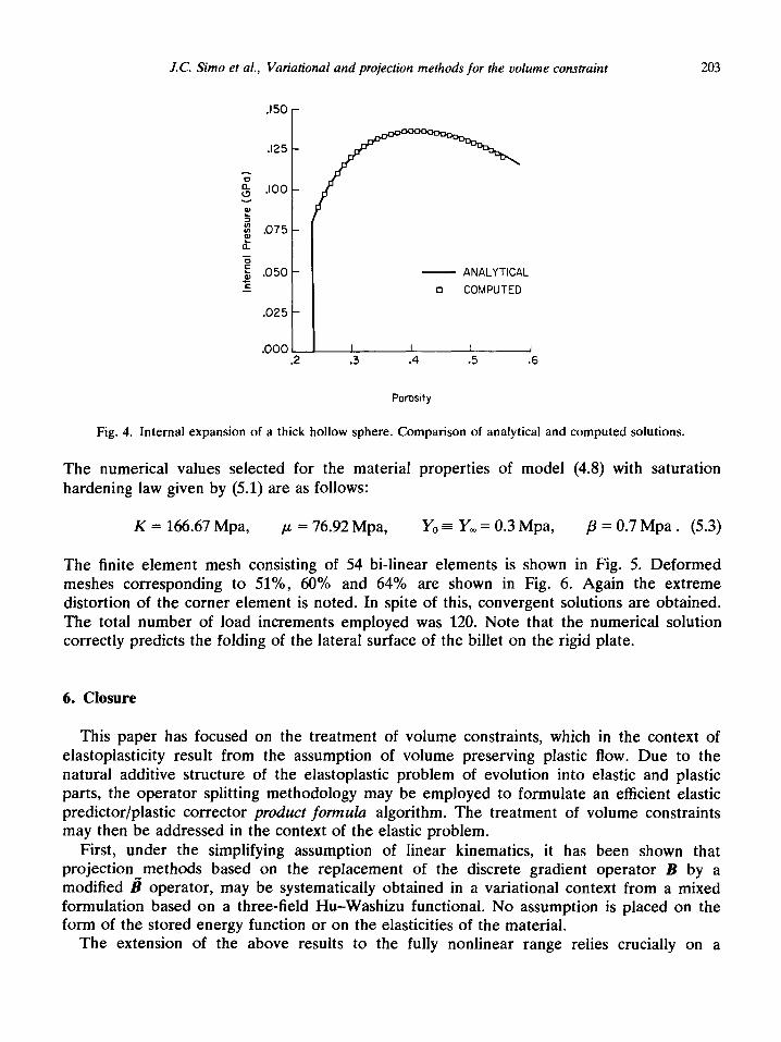
(2) I~te~~l expulsion of a twice hollow sphere. The purpose of this example is to compare the results obtained by numerical simulation, with one of the few available analytical results. If the assumption of negligible elastic deformations is introduced and, in addition, incompressible behavior is postulated, exact analytical solutions [S] may be obtained for hardening laws of the saturation type given by

K(ep)~ y,+(Y,- Yo)eoeP+@P, ~>O,P>O- (5.1)

The final element mesh ~o~esponding to a hollow sphere with inner and outer radius with values 12.5 m and 20 m is shown in Fig. 3. To allow comparison with the analytical result, numerical values of the material constants given below were selected to ensure ‘small’ elastic strains:

K = 800 Mpa, ,u = 300 Mpa, Y,, = 0.083 Mpa,

Y, = 0.486 Mpa, Q = 0.75 . (5.2)

Xn addition, we set fl= 0. The computed and analytical results are shown in Fig. 4, where the internal pressure has been plotted versus the change in porosity. The good agreement between both solutions is noted.

(3) Elastic-plastic upsetting of un &symmetric billet. Our final example is analogous to the first one considered in this section, with the difference that elasto-plastic response is now considered. This example was recently proposed as a severe test problem for current finite element formulation of finite deformation elastoplasticity (see [49] and references therein). The objective is to achieve 60% compression on a billet of 9 mm radius and 30 mm height.

12.5 m.

Fig. 3. Internal expansion of a thick hollow sphere. Finite element mesh. E-linear quadrilateral elements with constant pressure and constant Jacobian.


.I25

t

- ANALYTICAL

I3 COMPUTED

.2 .3 .4 .5 .6

Pomsity

Fig. 4. Internal expansion of a thick hollow sphere. Comparison of analytical and computed solutions.

The numerical values selected for the material properties of model (4.8) with saturation hardening law given by (5.1) are as follows:

K = 166.67 Mpa, ,u = 76.92 Mpa, Y0 = Y, = 0.3 Mpa, p = 0.7 Mpa . (5.3)

The finite element mesh consisting of 54 bi-linear elements is shown in Fig. 5. Deformed meshes corresponding to 51%, 60% and 64% are shown in Fig. 6. Again the extreme distortion of the corner element is noted. In spite of this, convergent solutions are obtained. The total number of load increments employed was 120. Note that the numerical solution correctly predicts the folding of the lateral surface of the billet on the rigid plate.

6. Closure

This paper has focused on the treatment of volume constraints, which in the context of elastoplasticity result from the assumption of volume preserving plastic flow. Due to the natural additive structure of the elastoplastic problem of evolution into elastic and plastic parts, the operator splitting methodology may be employed to formulate an efficient elastic predictor/plastic corrector product formula algorithm. The treatment of volume constraints may then be addressed in the context of the elastic problem.

First, under the simplifying assumption of linear kinematics, it has been shown that projection_methods based on the replacement of the discrete gradient operator B by a modified B operator, may be systematically obtained in a variational context from a mixed formulation based on a three-field Hu-Washizu functional. No assumption is placed on the form of the stored energy function or on the elasticities of the material.

The extension of the above results to the fully nonlinear range relies crucially on a


Upsetting of Axisymmetric Billet

15 mm

PLASTIC RESPONSE

Bulk = 166.67Mpa

G = 76.92 Mpa

s = 0.70Mpa

k = 0.30 Mpa

9mm (unilateral constrolnt)

Fig. 5. Elasto-plastic upsetting of a billet. Finite element mesh.

Upsetting of Axisymmetric Billet Upsetting of Axisymmetric Billet

t

I I I I 1

(unilateral constraint )

. Y

1 I I

(uniloterol constraint)

51% Compression Plastic Response

(4 60% Compression Plastic Response

(b)

Fig. 6. Elasto-plastic upsetting of a billet. (a) Deformed mesh corresponding to 51% compression. (b) Deformed mesh corresponding to 60% compression. (c) Deformed mesh corresponding to 64% compression.


Axisymmetric Billet

64% Compression Plastic Response (c)

Fig. 6 (contd).

multiplicative split of the deformation gradient into volume preserving and dilatational parts. A mixed formulation is then constructed on the basis of a three-field nonlinear Hu-Washizu principle. It has been shown that in contrast to the case of linearized kinematics, the tangent operator is not obtained by mere replacement of B by B. Additional terms appear as a result of the non-linear dependence of B on the configurations.

The volume-preserving/dilatational multiplicative split enjoys a clear physical interpretation and fits naturally in a formulation of plasticity based on the multiplicative decomposition. Application was made to a model problem for elastoplasticity which incorporates truly hyperelastic response and enables one to exactly satisfy the condition of volume preserving plastic flow. It is emphasized that hypoelastic characterizations, objective rates and incrementally objective algorithms play no role in the formulation and numerical treatment of the elastoplastic problem proposed here. In addition, one recovers an efficient treatment of hyperelasticity as a particular case, simply by assigning a large enough value to the yield stress.

Appendix A. Expression for r (u, q)

To carry out the calculation of f(u, q) first one needs to compute D[GRAD q,,] - ~0. To this end, observe that


D[Vq] - u. = D[-GRAD r),F-‘1 * u.

= -GRAD qoF-‘GRAD uoF-’

= -vqvu. (A4

Making use of this result in conjunction with (3.27) and definition (2.23) for Vq, it follows that

D[GRAD qo] - ~lo = D[VulT’] - u,

= [VqVu - VuVq + $(Vu : Vr/)g + ;(D[div q] . u,)g]k (A-2)

The calculation is completed by evaluating the contribution of D[z q] l uo. From definition (3.22) we have

D[div+h=--diVqdivu

= w(x) l H;’ 1 !@)[div u div IJ - Vu : Vq] dv . (A-3) n,

By making use of expression (3.21), for the pressure field and (A.3), the contribution of D[div q] - w, may be evaluated as

7:$D[divq].uodV= - f(trT)divudivq dV

= I pl[div u div q - VuVq] dv . (A.4) *(a)

Substitution of (A.2) and (A.4) into expression (3.33) for r(u, q) yields the desired result:

l== I ~[(VUC?): %j - (Vu@) : Vq] dv *U&j

+ $(tr ti)[Vu : Vq - div udiv q] dv

+ pa[div u div q - Vu : Vq] dv .

Acknowledgment

(A-5)

We thank Professors T.J.R. Hughes and J. Lubliner for helpful discussions.


References

[l] J. Argyris, An excursion through large rotations, Comput. Meths. Appl. Mech. Engrg. 32 (1982) 85-155. [2] J.H. Argyris and JSt. Doltsinis, On the large strain inelastic analysis in natural formulation-Part I.

Quasistatic problems, Comput. Meths. Appl. Mech. Engrg. 20 (1979) 213-252. [3] J.H. Argyris and J.St. Doltsinis, On the large strain inelastic analysis on natural formulation -Part II. Dynamic

problems, Comput. Meths. Appl. Mech. Engrg. 21 (1980) 91-126. [4] J.H. Argyris, J.St. Doltsinis, P.M. Pimenta and H. Wiistenberg, Thermomechanical response of solids at high

strains-Natural approach, Comput. Meths. Appl. Mech. Engrg. 32 (1982) 3-57. [5] V.I. Arnold, Mathematical Methods of Classical Mechanics (Springer, New York, 1980). [6] T. Belytschko, J.S. Ong, W.K. Liu and J.M. Kennedy, Hourglass control in linear and nonliner problems,

Comput. Meths. Appl. Mech. Engrg. 43 (1984) 251-276. [7] J. Carey and J.T. Oden, Finite Element, Vol. II, Texas Series in Computational Mechanics (Prentice-Hall,

Englewood Cliffs, NJ, 1983). [8] M.M. Carroll, Radial expansion of hollow spheres of elastic-plastic hardening material, preprint, 1985. [9] P.J. Flory, Thermodynamic relations for high elastic materials, Trans. Faraday Sot. 57 (1961) 829-838.

[lo] M. Fortin, Old and new elements for incompressible flows, Rept. No. MPA21, Collection Mathematique, Universite Laval, Quebec, Canada.

[ll] M. Fortin and R. Glowinsky, Resolution numerique de problemes aux limites par des methodes de Lagrangient augmente, in: Methodes Mathematiques de L’informatique (Dunod-Bordas, Paris, 1982).

[12] J.O. Hallquist, NIKE2D: An implicit, finite deformation, finite element code for analyzing the static and dynamic response of two dimensional solids, Rept. UCRL-52678, Lawrence Livermore National Laboratory, University of California, Livermore.

[13] L.R. Herrmann, Elasticity equations for incompressible and nearly incompressible materials by a variational theorem, AIAA J. 3 (10) (1965).

[14] T.J.R. Hughes, Equivalence of finite elements for nearly incompressible elasticity, J. Appl. Mech. (1977) 181-183.

[15] T.J.R. Hughes, Generalization of selective integration procedures to anisotropic and nonlinear media, Internat. J. Numer. Meths. Engrg. 15 (9) (1980) 1413-1418.

[16] T.J.R. Hughes, W.K. Liu and A. Brooks, Review of finite element analysis of incompressible viscous flows by the penalty function formulation, J. Comput. Phys. 30 (1979) l-60.

[17] T.J.R. Hughes and D.S. Malkus, A general penalty/mixed equivalence theorem for anisotropic incompressible elements, in: N. Atluri, R. Gallager and 0. Zienkiewicz, eds., Hybrid and Mixed Finite Element Methods (Wiley, New York, 1983).

[18] T.J.R. Hughes and J. Winget, Finite rotation effects in numerical integration of rate constitutive equations arising in large-deformation analysis, Internat. J. Numer. Meths. Engrg. 15 (9) (1980) 1413-1418.

[19] D.W. Iwan and P.J. Yoder, Computational aspects of strain-space plasticity, J. Engrg. Mech., AXE 109 (1983) 231-243.

[20] S. Key, A variational principle for incompressible and nearly incompressible anisotropic elasticity, Internat. J.

WI

WI

]231 ]241

]251

P61

[271

Solids Structures 5 (1969) 951-964. N. Kikuchi and Y.J. Song, Remarks on relations between penalty and mixed finite element methods for a class of variational inequalities, Internat. J. Numer. Meths. Engrg. 15 (1980) 1557-1579. R.D. Krieg and D.B. Krieg, Accuracies of numerical solution methods for the elastic-perfectly plastic model, J. Pressure Vessel Tech., ASME 99 (1977). E.H. Lee, Elastic-plastic deformation at finite strains, J. Appl. Mech. 36 (1%9). D.S. Malkus, Finite elements with penalties in nonlinear elasticity, Internat J. Numer. Meths. Engrg. 16 (1980) 121-136. D.S. Malkus, Eigenproblems associated with the discrete condition for incompressible finite elements, Internat. J. Engrg. Sci. 19 (1981) 1299-1310. D.S. Malkus and T.J.R. Hughes, Mixed finite element methods -Reduced and selective integration techniques: A unification of concepts, Comput. Meths. Appl. Mech. Engrg. 15 (1978) 63-81. J.E. Marsden and T.J.R. Hughes, Mathematical Foundations of Elasticity (Prentice-Hall, Englewood Cliffs, NJ, 1983).


[28] W.C. Moss, On the computational significance of the strain space formulation of plasticity theory, Internat. J. Numer. Meths. Engrg. 20 (1984) 1703-1709.

[29] J.C. Nagtegaal, On the implementation of inelastic constitutive equations with special reference to large deformation problems, Comput. Meths. Appl. Mech. Engrg. 33 (1982) 469-484.

[30] J.C. Nagtegaal, D.M. Parks and J.R. Rice, On numerically accurate finite element solutions in the fully plastic range, Comput. Meths. Appl. Mech. Engrg 4 (1974) 153-177.

[31] J.T. Oden, RIP-methods for Stokesian flows, TICOM Rept. 80-11, The University of Texas at Austin. [32] J.T. Oden and N. Kikuchi, Finite element methods for constrained problems in elasticity, Internat. J. Numer.

Meths. Engrg. (1982) 701-725. [33] J.T. Oden, N. Kikuchi and Y.J. Song, Penalty-finite element methods for the analysis of Stokesian flows,

Comput. Meths. Appl. Mech. Engrg. 31 (1982) 297-329. [34] R.W. Ogden, Elastic deformations of rubber-like solids, in: H.G. Hopkins and M.J. Sewell, eds., Mechanics of

Solids, R. Hill 60th Anniversary Volume (1982) 499-537. [35] P.M. Pinsky, M. Ortiz and K.S. Pister, Numerical integration of rate constitutive equations in finite

deformation analysis, Comput. Meths. Appl. Mech. Engrg. 40 (1983) 137-158. [36] J. Pitkaranta and R. Stenberg, Error bounds for the approximation of the Stokes problem using bilinear/con-

stant elements on irregular quadrilateral meshes, Rept. MAT-A222, Helsinki University of Technology. [37] J.N. Reddy, On penalty function methods in the finite element analysis of flow problems, Internat. J. Numer.

Meths. Fluids 2 (1982) 151-171. [38] E. Reissner, On a variational principle for elastic displacements and pressure, J. Appl. Mech. 51 (1983)

444-445. [39] R. Rubinstein and S.N. Atluri, Objectivity of incremental constitutive relations over finite time steps in

computational finite deformation analyses, Comput. Meths. Appl. Mech. Engrg. 36 (1983) 277-290. [40] H.L. Schreyer, R.L. Kulak and J.M. Kramer, Accurate numerical solutions for elastic-plastic models, J.

Pressure Vessel Tech., ASME 101 (1979). [41] B.F. Schutz, Geometrical Methods of Mathematical Physics (Cambridge University Press, Cambridge, 1980). [42] J.C. Simo and J.E. Marsden, Stress tensors, Riemannian metrics and alternative representations of elasticity,

in: Trends in the Application of Mathematics to Mechanics, Lecture Notes in Physics (Springer, Berlin, 1983). [43] J.C. Simo and J.E. Marsen, On the rotated stress tensor and the material version of the Doyle-Ericksen

formula, Arch. Rat. Mech. Anal. 86 (3) (1984) 213-231. [44] J.C. Simo and M. Ortiz, A unified approach to finite deformation elastoplasticity based on the use of hyperelastic

constitutive equations, Comput. Meths. Appl. Mech. Engrg. 49 (1985) 221-245.

(451 J.C. Simo and K.S. Pister, Remarks on rate constitutive equations for finite deformation problems: Com- putational implications, Comput. Meths. Appl. Mech. Engrg. 46 (1984) 201-215.

[46] J.C. Simo and R.L. Taylor, Consistent tangent operators for rate independent elasto-plasticity, Comput. Meths. Appl. Mech. Engrg. 48 (1985) 101-118.

[47] J.C. Simo, P. Wriggers and R.L. Taylor, A perturbed Lagrangian formulation for the finite element solution of contact problems, Comput. Meths. Appl. Mech. Engrg. 50 (1985) 163-180.

[48] Y.J. Song, J.T. Oden and N. Kikuchi, Discrete LBB-conditions for RIP-finite element methods, TICOM Rept. 80-7, The University of Texas at Austin.

[49] L.M. Taylor and E.B. Becker, Some computational aspects of large deformation, rate-dependent plasticity problems, Comput. Meths. Appl. Mech. Engrg. 41 (1983) 251-278.

[50] R.L. Taylor, K.S. Pister and L.R. Hermann, A variational principle for incompressible and nearly-incompressible orthotropic elasticity, Internat. J. Solids Structures 4 (1968) 875-883.

[51] C. Truesdell and W. Noll, The Non-Linear Field Theories of Mechanics, in: S. Flugge, ed., Handbuch der Physik, Vol. III/3 (Springer, Berlin, 1965).

[52] O.C. Zienkiewicz and S. Nakazawa, The penalty function method and its applications to the numerical solution of boundary value problems, in: Winter Annual ASME Meeting (1983).

[53] O.C. Zienkiewicz, R.L. Taylor and J.M.W. Baynham, Mixed and irreducible formulations in finite element analysis, in: S.N. Atluri, R.N. Gallagher and O.C. Zienkiewicz, eds., Hybrid and Mixed Finite Element Methods (Wiley, New York, 1983).

variational and projection methods for the …

Documents