variations of the star schema benchmark to test the

Variations of the Star Schema Benchmark to Test theEffects of Data Skew on Query Performance

Tilmann RablMiddleware Systems

Reseach GroupUniversity of Toronto

Ontario, [email protected]

Meikel PoessOracle Corporation

Califonia, [email protected]

Hans-Arno JacobsenMiddleware Systems

Research GroupUniversity of Toronto

Ontario, [email protected]

Patrick O’NeilDepartment of Math and C.S.University of Massachusetts

BostonMassachusetts, USA

[email protected]

Elizabeth O’NeilDepartment of Math and C.S.University of Massachusetts

BostonMassachusetts, USA

[email protected]

ABSTRACT

The Star Schema Benchmark (SSB), has been widely used toevaluate the performance of database management systemswhen executing star schema queries. SSB, based on the wellknown industry standard benchmark TPC-H, shares some ofits drawbacks, most notably, its uniform data distributions.Today’s systems rely heavily on sophisticated cost-basedquery optimizers to generate the most efficient query exe-cution plans. A benchmark that evaluates optimizer’s capa-bility to generate optimal execution plans under all circum-stances must provide the rich data set details on which op-timizers rely (uniform and non-uniform distributions, datasparsity, etc.). This is also true for other database systemparts, such as indices and operators, and ultimately holdsfor an end-to-end benchmark as well. SSB’s data generator,based on TPC-H’s dbgen, is not easy to adapt to differentdata distributions as its meta data and actual data genera-tion implementations are not separated. In this paper, wemotivate the need for a new revision of SSB that includesnon-uniform data distributions. We list what specific modi-fications are required to SSB to implement non-uniform datasets and we demonstrate how to implement these modifica-tions in the Parallel Data Generator Framework to generateboth the data and query sets.

Categories and Subject Descriptors

K.6.2 [Management of Computing and InformationSystems]: Installation Management—benchmark, perfor-

mance and usage measurement

Permission to make digital or hard copies of all or part of this work forpersonal or classroom use is granted without fee provided that copies arenot made or distributed for profit or commercial advantage and that copiesbear this notice and the full citation on the first page. To copy otherwise, torepublish, to post on servers or to redistribute to lists, requires prior specificpermission and/or a fee.ICPE’13, March 21–24, 2013, Prague, Czech Republic.Copyright 2013 ACM 978-1-4503-1636-1/13/03 ...$15.00.

Keywords

Star Schema Benchmark; PDGF; data skew; data genera-tion; TPC-H

1. INTRODUCTIONTraditionally, relational schemas were designed using data-

base normalization techniques pioneered by Edgar F. Codd[4]. Database normalization minimizes data redundancy anddata dependencies. However, Kimball argues that this tra-ditional approach to designing schemas is not suitable fordecision support systems because of poor query performanceand usability [7]. He further argues that the design of a de-cision support system should follow a star schema, whichfeatures a fact table containing real live events, e.g., sales,returns etc., and dimensions further describing these eventsby supplying attributes such as sales price, item descriptionsetc. While traditional normalized schemas are designed toreduce the overhead of updates, star schemas are designed toincrease the ease-of-use and speed of retrieval. These funda-mental design goals are achieved by minimizing the numberof tables that need to be joined by queries.

Having realized the need to measure the performance ofdecision support systems in the early 1990s, the TransactionProcessing Performance Council (TPC) released its first de-cision support benchmark, TPC-D, in April 1994. Becauseat that time the majority of systems followed Codd’s nor-malization approach, TPC-D is based on a 3rd normal formschema consisting of 8 tables. Even TPC-H, TPC-D’s suc-cessor, which was released in April 1999 continued using thesame 3rd normal form schema.

While for the technology available at that time, TPC-Dand TPC-H imposed many challenges, both on hardwareand on database management systems (DBMS). However,their 3rd normal form schema and uniform data distribu-tions are not representative any more of current decisionsupport systems. As a consequence, O’Neil et al. proposed astar schema version of TPC-H, the Star Schema Benchmark(SSB) in [11]. SSB denormalizes the data that TPC-H’sdata generator, dbgen, generates. However, its underlying

14 16 18 20 22 24 26 28 30 32 34

2 4 6 8 10 12

Sal

es in

Bill

ion

US

Dol

lars

Month

Figure 1: US Retail Sales in Billion US Dollars asReported by the US Cenus

data generation principles were not changed from TPC-H,especially its uniform data distributions.We argue that uniform data distributions are not repre-

sentative for real life systems because of naturally occur-ring data skew. For instance, retail sales tend to be highlyskewed towards the end of the year, customers are clusteredin densely populated areas and popular items are sold moreoften than unpopular items.Non-uniform data distributions impose great challenges

to database management systems. For instance, data place-

ment algorithms, especially those on large scale shared noth-ing systems, are sensitive to data skew, but also commonoperations such as join, group-by and sort operations canbe affected by data skew, most notably the query optimizer,is highly challenged to generate the optimal execution planfor queries in the presence of data skew. This is supportedin a SIGMOD 1997 presentation by Levine and Stephens inwhich they noted that a successor of TPC-D should includedata skew [2].Consider the retail sales numbers per month as reported

by the US census in Figure 1. The graph shows that USretail sales vary between 15 Billion in January and 35 Billionin December. Sales stay under 20 Billion per month untilNovember when they shoot to 25 Billion and then to 35Billion in December. It is not uncommon that during theyear-end holiday season, often as much as 30% of annualsales are made within the last two months of the year (andmuch of that in the last half of December) [14].TPC-DS, published in April 2012, includes some data

skew [10], implemented using “comparability zones”, whichare ranges in the data domain of columns with uniform dis-tributions. The number of comparability zones for a partic-ular column is limited only by the number of unique valuesin this column. However, because of the underlying designprinciples of TPC-DS, execution of individual queries is re-stricted to one comparability zone. While TPC-DS’s ap-proach for data skew is a step in the right direction, it limitsthe effect of data skew greatly, because individual queriesstill operate on uniform data.So far there has not been any industry standard bench-

mark that tests query performance in the presence of highlyskewed data. This paper addresses the need for a modern de-cision support benchmark that includes highly skewed data.The resulting new version of SSB includes data skew in singlefact table measures, single dimension hierarchies and mul-tiple dimension hierarchies. To demonstrate the effects ofdata skew on query performance, several experiments were

run on a publicly available DBMS. The results of these ex-periments underline the need for the introduction of dataskew in SSB.

Because SSB’s current data generator is an adapted ver-sion of TPC-H’s data generator, which hard codes mostof the data characteristics, a new data generator was im-plemented using the Parallel Data Generation Framework(PDGF). It’s design allows for quickly modifying data dis-tributions as well as making structural changes to the ex-isting tables. In addition it allows the generation of validSQL from query templates similar to qgen of SSB. Thisis particularly important as PDGF allows for the genera-tion of queries in the presence of data skew. While thispaper demonstrate the key aspects of the data generator,the fully functional data generator is available at http:

//www.paralledatageneration.org/.In summary, our contributions in this paper are:

• We design and implement a complete data genera-tor for SSB based on the Parallel Data GenerationFramework (PDGF) that can be easily adapted andextended.

• We design and implement a query generator for SSBbased on PDGF, which enables the generation of morerealistic queries with parameters that originate fromthe data set rather than randomly chosen values.

• We introduce skew into SSB’s data model in a consis-tent way, which makes it possible to reason about theselectivity of queries.

• We implement the proposed data skew in our data gen-erator and demonstrate the effects of the skew on queryprocessing times.

The remainder of this paper is organized as follows. Sec-tion 2 reviews those parts of SSB that are relevant to un-derstanding the concepts discussed in this paper. Section 3presents our data and query generator implementations inPDGF. Section 4 suggests and discusses variations of thestar schema benchmark that include various degrees of dataskew including experimental results. Before concluding ourpaper, we discuss related work in Section 5.

2. STAR SCHEMA BENCHMARKThe Star Schema Benchmark is a variation of the well

studied TPC-H benchmark [12], which models the data ware-house of a whole sale supplier. TPC-H models the data in3rd normal form, while SSB implements the same logicaldata in a traditional star schema, where the central fact ta-ble Lineorder contains the ”sales transaction information“ ofthe modeled retailer in form of different types of measuresas described in [7]. SSB’s queries are simplified versions ofthe queries in TPC-H. They are organized in four flights ofthree to four queries each.

This paper focuses on data skew in columns that are usedfor selectivity predicates because data skew in those columnsexhibit the largest impact on query performance. Hence, thedata set and query set need to be considered when introduc-ing skew into SSB. Therefore, the following two sections firstrecap the main characteristics of SSB’s schema and data setand then analyze the four query flights to ultimately suggesta representative set of columns for which data skew couldbe implemented.

Figure 2: SSB Schema

The uniform characteristics of the TPC-H [1] data set havebeen studied extensively in [13]. According to the TPC-Hspecification the term “random” means “independently se-lected and uniformly distributed over the specified rangeof values” . That is, n unique values V of a column areuniformly distributed if P (V = v) = 1

n. Because TPC-H

and SSB’s data generators use pseudo random number gen-erators and data is generated independently in parallel onmultiple computers, perfectly uniform data distributions areimpossible to guarantee. Hence, we follow the definition ofuniform as presented in [13].

2.1 SSB Schema and Data PopulationIn order to create a star schema of TPC-H, SSB denor-

malizes several tables: (i) the Order and Lineitem tables aredenormalized into a single Lineorder fact table and (ii) theNation and Region tables are denormalized into the Cus-tomer and Supplier tables and a city column is added. Thissimplifies the schema considerably, both for writing queriesand computing queries as the two largest tables of TPC-Hare pre-joined. Queries do not have to perform the join andusers writing queries against the schema do not have to ex-press the join in their queries. In SSB, the Partsupp table isremoved, because this table has a different temporal gran-ularity than the Lineorder table. This is an inconsistencyin the original TPC-D and TPC-H schemas as described in[11]. Finally, an additional Date table is added, which iscommonly used in star schemas. To summarize, SSB con-sists of one large fact table (Lineorder) and four dimensions(Customer, Supplier, Part, Date). The complete schema isdepicted in Figure 2.Like in TPC-H, all data in SSB is uniformly distributed.

To be consistent with the general star schema approach thedefinition of the SSB tables is slightly different from thedefinition of TPC-H. The most notable change is the in-troduction of selectivity hierarchies in all dimension tables.They are similar to the manufacturer/brand hierarchy inTPC-H, where the manufacturer (P Mfgr) value is a prefixof the brand (P Brand) value. We denote this dependencywith P Brand → P Mfgr, meaning that for each P Brandvalue there is exactly one P Mfgr value. In the Part table,SSB adds a category, which extends the TPC-H hierarchyto P Brand1 → P Category → P Mfgr. Because all data isuniformly distributed this hierarchy serves as a simple wayto control row selectivity of queries. There are five differ-ent values for P Mfgr, resulting in selectivity of 1

5each. For

each of those there exist five different values in P Categorywith a selectivity of 1

25each. Finally, the P Brand1 field

has 40 variations per P Category value for a selectivity of1

1000each. The hierarchies in Customer and Supplier are

C City → C Nation → C Region and S City → S Nation→ S Region, respectively. Date features two natural hi-erarchies D DayNumInMonth → D Month → D Year andD DayNumInWeek → D Week → D Year .

2.2 SSB QueriesInstead of TPC-H’s 22 queries, O’Neil et al. propose four

flights of queries that each consist of three to four querieswith varying selectivity [11]. Each flight consists of a se-quence of queries that someone working with data warehousesystem would ask, e.g., for a drill down.

Query Flight 1 (Q1.1, Q1.2 and Q1.3) is based on TPC-H’s Query 6 (see Listing 1 for the SQL code of Q1.1). Itperforms a single join between the Lineorder table and thesmall Date dimension table. Selectivity predicates are seton D Year, Lo Discount and Lo Quantity. Flight 1 simu-lates a drill down into the Date dimension. From one queryof the flight to the next join selectivity is reduced by re-fining the predicate on the Date component. Q1.1’s Daterange is one year, Q1.2 selects data within a range of onemonth and Q1.3’s refines this further by selecting data of oneweek. Q1.3 further changes the predicate on Lo Quantityfrom less than n to between n and m.

SELECT SUM(lo_extendedprice*lo_discount) AS revenueFROM lineorder , date

WHERE lo_orderdate = d_datekeyAND d_year = 1993AND lo_discount BETWEEN 1 AND 3AND lo_quantity < 25;

Listing 1: Query Q1.1 of SSB

In order to measure the effect of data skew on query ex-ecution times of queries in Flight 1, we propose data skewin (i) Lo Orderdate, (ii) Lo Discount and (iii) Lo Quantity.Data skew in the Lo Orderdate column is realistic as retailsales are low and flat in the summer, but pick up steeply afterThanksgiving to top in December (see Figure 1). Data Skewin Lo Discount and Lo Quantity are also realistic, which canbe categorized as single column skew of single tables becausethese columns are statistically independent.

Queries in Flight 2 join the Lineorder, Date, Part andSupplier tables (see Listing 2 for Q2.1). They aggregate andsort data on Year and Brand. Selectivity is modified usingpredicates on P Category, S Region and P Brand. That is,they use the P Brand1 → P Category → P Mfgr hierarchyin the Part table.

SELECT SUM(lo_revenue), d_year , p_brand1FROM lineorder , date , part , supplier

WHERE lo_orderdate = d_datekeyAND lo_partkey = p_partkeyAND lo_suppkey = s_suppkeyAND p_category = ’MFGR #12’AND s_region = ’AMERICA ’

GROUP BY d_year , p_brand1ORDER BY d_year , p_brand1;


In addition to data skew in Lo Orderdate, as proposed forFlight 1, for Flight 2 we propose data skew in P Categoryand S Region, which is realistic as not every manufacturerproduces the same number of parts and not all suppliers aredistributed uniformly in all regions.Flight 3 aggregates revenue data by Customer and Sup-

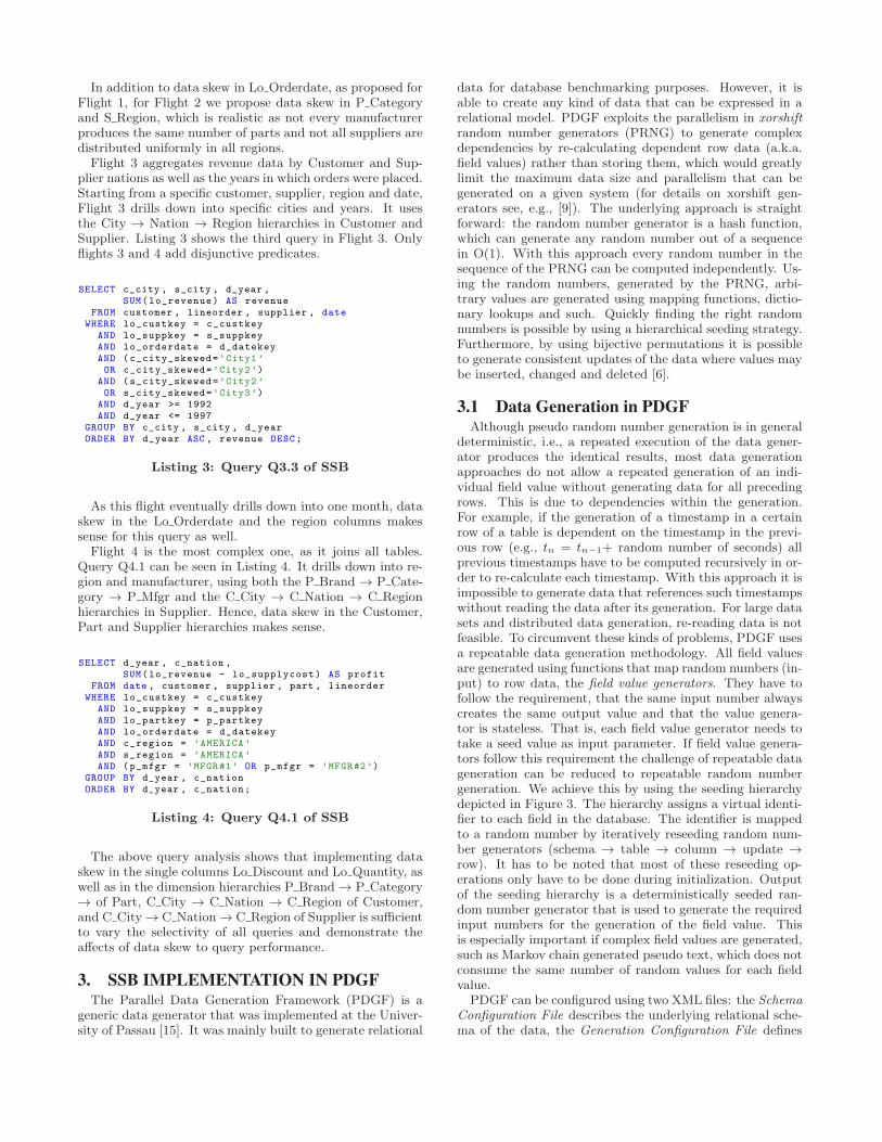
plier nations as well as the years in which orders were placed.Starting from a specific customer, supplier, region and date,Flight 3 drills down into specific cities and years. It usesthe City → Nation → Region hierarchies in Customer andSupplier. Listing 3 shows the third query in Flight 3. Onlyflights 3 and 4 add disjunctive predicates.

SELECT c_city , s_city , d_year ,SUM(lo_revenue) AS revenue

FROM customer , lineorder , supplier , dateWHERE lo_custkey = c_custkey

AND lo_suppkey = s_suppkeyAND lo_orderdate = d_datekeyAND (c_city_skewed=’City1’OR c_city_skewed=’City2’)

AND (s_city_skewed=’City2’OR s_city_skewed=’City3’)

AND d_year >= 1992AND d_year <= 1997

GROUP BY c_city , s_city , d_yearORDER BY d_year ASC , revenue DESC;


As this flight eventually drills down into one month, dataskew in the Lo Orderdate and the region columns makessense for this query as well.Flight 4 is the most complex one, as it joins all tables.

Query Q4.1 can be seen in Listing 4. It drills down into re-gion and manufacturer, using both the P Brand → P Cate-gory → P Mfgr and the C City → C Nation → C Regionhierarchies in Supplier. Hence, data skew in the Customer,Part and Supplier hierarchies makes sense.

SELECT d_year , c_nation ,SUM(lo_revenue - lo_supplycost) AS profit

FROM date , customer , supplier , part , lineorderWHERE lo_custkey = c_custkey

AND lo_suppkey = s_suppkeyAND lo_partkey = p_partkeyAND lo_orderdate = d_datekeyAND c_region = ’AMERICA ’AND s_region = ’AMERICA ’AND (p_mfgr = ’MFGR#1’ OR p_mfgr = ’MFGR#2’)

GROUP BY d_year , c_nationORDER BY d_year , c_nation;


The above query analysis shows that implementing dataskew in the single columns Lo Discount and Lo Quantity, aswell as in the dimension hierarchies P Brand → P Category→ of Part, C City → C Nation → C Region of Customer,and C City→ C Nation→ C Region of Supplier is sufficientto vary the selectivity of all queries and demonstrate theaffects of data skew to query performance.

3. SSB IMPLEMENTATION IN PDGFThe Parallel Data Generation Framework (PDGF) is a

generic data generator that was implemented at the Univer-sity of Passau [15]. It was mainly built to generate relational

data for database benchmarking purposes. However, it isable to create any kind of data that can be expressed in arelational model. PDGF exploits the parallelism in xorshift

random number generators (PRNG) to generate complexdependencies by re-calculating dependent row data (a.k.a.field values) rather than storing them, which would greatlylimit the maximum data size and parallelism that can begenerated on a given system (for details on xorshift gen-erators see, e.g., [9]). The underlying approach is straightforward: the random number generator is a hash function,which can generate any random number out of a sequencein O(1). With this approach every random number in thesequence of the PRNG can be computed independently. Us-ing the random numbers, generated by the PRNG, arbi-trary values are generated using mapping functions, dictio-nary lookups and such. Quickly finding the right randomnumbers is possible by using a hierarchical seeding strategy.Furthermore, by using bijective permutations it is possibleto generate consistent updates of the data where values maybe inserted, changed and deleted [6].

3.1 Data Generation in PDGFAlthough pseudo random number generation is in general

deterministic, i.e., a repeated execution of the data gener-ator produces the identical results, most data generationapproaches do not allow a repeated generation of an indi-vidual field value without generating data for all precedingrows. This is due to dependencies within the generation.For example, if the generation of a timestamp in a certainrow of a table is dependent on the timestamp in the previ-ous row (e.g., tn = tn−1+ random number of seconds) allprevious timestamps have to be computed recursively in or-der to re-calculate each timestamp. With this approach it isimpossible to generate data that references such timestampswithout reading the data after its generation. For large datasets and distributed data generation, re-reading data is notfeasible. To circumvent these kinds of problems, PDGF usesa repeatable data generation methodology. All field valuesare generated using functions that map random numbers (in-put) to row data, the field value generators. They have tofollow the requirement, that the same input number alwayscreates the same output value and that the value genera-tor is stateless. That is, each field value generator needs totake a seed value as input parameter. If field value genera-tors follow this requirement the challenge of repeatable datageneration can be reduced to repeatable random numbergeneration. We achieve this by using the seeding hierarchydepicted in Figure 3. The hierarchy assigns a virtual identi-fier to each field in the database. The identifier is mappedto a random number by iteratively reseeding random num-ber generators (schema → table → column → update →row). It has to be noted that most of these reseeding op-erations only have to be done during initialization. Outputof the seeding hierarchy is a deterministically seeded ran-dom number generator that is used to generate the requiredinput numbers for the generation of the field value. Thisis especially important if complex field values are generated,such as Markov chain generated pseudo text, which does notconsume the same number of random values for each fieldvalue.

PDGF can be configured using two XML files: the Schema

Configuration File describes the underlying relational sche-ma of the data, the Generation Configuration File defines

��

� ��

��

�

�

��

��

��

��

�

��

Figure 3: PDGF’s Seeding Strategy

how the data is formatted. The schema configuration hasa similar structure as the SQL definition of a relationalschema, it defines a set of tables which consist of fields. Eachfield has name, size, data type and generation specification.Listing 5 shows the first two fields of the Supplier table andthe definition of dependencies in PDGF. For instance, theS Name field is defined as the string “Supplier”, concate-nated with the value of the field S Suppkey and padded to 9places. PDGF automatically resolves this dependency if theOtherFieldValueGenerator is used. The additional transfor-mations can be specified with meta-generators that changethe values generated by subsequent generators. In the ex-ample, the padding is done by a PaddingGenerator and theprefix is added with another generator.

<table name="SUPPLIER"><size>${S}</size>

<field name="S_SUPPKEY" size="" type="NUMERIC"primary="true" unique="true">

<gen_IdGenerator /></field>

<field name="S_NAME" size="25" type="VARCHAR"><gen_PrePostfixGenerator>

<gen_PaddingGenerator ><gen_OtherFieldValueGenerator >

<reference field="S_SUPPKEY" /></gen_OtherFieldValueGenerator ><character >0</character ><padToLeft >true</padToLeft ><size>9</size>

</gen_PaddingGenerator ><prefix>Supplier </prefix>

</gen_PrePostfixGenerator></field>

[..]

Listing 5: Excerpt of the Supplier Table Definition

One peculiarity of the SSB schema is the definition of theLineorder table. It resembles the denormalized Lineitem↔ Order relationship of TPC-H. One row in the Order ta-ble corresponds to n ∈ [1, 7] rows in the Lineitem table.In its denormalized version each row of the Lineorder ta-ble contains the individual price of the item as well as thetotal price of the order. Hence, there is a linear depen-dency between Lineitem and Orders. This is resolved inPDGF in the following way: Instead of treating each lineitem as a single row we generate all line items of a par-ticular order in one row. This is similar to the genera-tion of Lineorder in the original generator of SSB and thegeneration of Lineitem and Order in TPC-H, respectively.The PDGF implementation of Lineorder ist shown in List-ing 6. The field Lo Number Of Lineitems determines thenumber of lineitems within a certain order. This field isnot printed. All order related values, e.g., Lo Orderkey, are

specified once, while values that are specific to a lineitem,e.g., Lo Linenumber are specified for each lineitem.

<table name="LINEORDER"><size>${L}</size>

<field name="LO_ORDERKEY" size=""type="NUMERIC"><gen_FormulaGenerator >

<formula >(gc.getID() / 8 * 32) +

(gc.getID() % 8)</formula ><decimalPlaces >0</decimalPlaces >

</gen_FormulaGenerator ></field>

<field name="LO_NUMBER_OF_LINEITEMS" size=""type="NUMERIC"><gen_LongGenerator>

<min>1</min><max>7</max>

</gen_LongGenerator></field>

<field name="LO_LINENUMBER_1" size=""type="NUMERIC"><gen_StaticValueGenerator>

<value>1</value></gen_StaticValueGenerator>

</field>[..]

Listing 6: Excerpt of the Lineorder Table Definition

The output of Lineorder data as multiple rows is specifiedin the generation configuration file, which describes the out-put location and format of the output data. Furthermore,the generation configuration file allows for specifying arbi-trary post-processing operations. In Listing 7, an excerptof the generation specification for Lineorder is shown. Thevalue of the field in Column 2, Lo Number Of Lineitems,determines the number of rows that have to be generated.

<table name="LINEORDER" exclude="false"><output name="CompiledTemplateOutput"><fileTemplate >outputDir + table.getName ()

+ fileEnding </ fileTemplate ><outputDir >output/</outputDir ><fileEnding >.tbl </fileEnding ><charset >UTF -8</charset ><sortByRowID >true </ sortByRowID ><template ><!--

int noRows=( fields [1]. getPlainValue ()).intValue ();

for (int i = 0; i < noRows; i++) {buffer.append( fields [0] ); // LO_ORDERKEY

buffer.append(’|’).append( fields [2+i] );[..]

Listing 7: Excerpt of the Generation Definition forLineorder

Post-processing in the generation configuration, as shownin Listing 7, is only necessary if the relational definition inthe schema definition file is not identical to the format ondisk.

Another example in the SSB schema is the address infor-mation. Because the dimension tables are denormalized theRegion and Nation fields have to be generated consistently(e.g., France should always be in Europe). We implementedthis by specifying a virtual table Region Nation, which is

referenced by other tables and is not actually generated.This way, we ensure consistency in the data generation be-cause the virtual table Region Nation contains only validRegion-Nation combinations.

3.2 Query Generation in PDGFIn addition to the data generation, we also designed and

implemented a query generator in PDGF, which convertsthe SSB query templates into valid SQL. In order to gener-ate a large query set, many benchmarks including TPC-H,TPC-DS and SSB define query templates that can be con-verted into valid SQL queries. For TPC-H and TPC-DS thisis done by tools that substitute tagged portions of querieswith valid values, such as selectivity predicates, aggregationfunctions or columns (qgen, DSQgen) [14].In order for suchtools to generate a valid and predictable workload they needto have knowledge about the schema and data set. Oth-erwise the chosen values, e.g., selectivity predicates mightnot qualify the desired number of rows. TPC-H’s qgen andits counterpart for SSB generate queries by selecting ran-dom values within the possible ranges of the data. Thefollowing shows the definition of the supplier name rangesas specified in the TPC-H specification: S_NAME text ap-

pended with digit ["Supplier", S_SUPPKEY]

TPC-H’s and SSB’s qgen implementations have majordrawbacks: (i) the parameter ranges for each substitutionparameter are hard-coded into a c-program, (ii) scale factordependent substitution parameter handing is difficult, and(iii) this approach only works on uniformly distributed data.Instead of hard-coding valid parameter ranges for each

query, we use PDGF’s post-processing functionality to im-plement our query generator for SSB. For each query wedefine one table that is populated with all valid parametersof that query. We refer to these tables as parameter tables.The key benefit of our approach is that query parametersare generated from existing values in the data set. Usingour approach we generate queries by selecting random fieldvalues from the data set, i.e., field values that actually existin the generated data. This is a more flexible approach as itdoes not statically define the data range.In Listing 8, an excerpt for the table specifying the pa-

rameters for Query Q1.1 can be seen.

<table name="QUERYPARAMETERS_Q1 .1"><size>13 * ${ QUERY_ROUNDS}</size><field name="YEAR" size="4" type="NUMERIC">

<gen_LongGenerator><min>1993</min><max>1997</max>

</gen_LongGenerator></field>

[..]</table>

Listing 8: Schema Definition of the Parameter Tablefor Query Q1.1 (excerpt)

The query template itself is specified in the generationconfiguration. For Query Q1.1 this can be seen in Listing 9.As can be seen in the listing, the template is embedded in aXML comment in Java-style String format. This format willbe compiled into a regular Java binary at runtime. Futureversions of PDGF will include a new output plugin that isable to read the template from files and directly generatethis Java representation.

<table name="QUERY_PARAMETERS" exclude="false" ><output name="CompiledTemplateOutput" >

[..]<template ></template ></output >

</table >

Listing 9: Excerpt of the Template Specification forQuery Q1.1

4. STAR SCHEMA BENCHMARK VARIA-

TIONSOur PDGF implementation of the original Star Schema

Benchmark enables easy alterations to the schema and thedata generation as well as the query generation. Columnscan be easily added or data distributions changed and queriesmodified and added. This section discusses different ap-proaches of introducing data skew into the original SSB andthe reasoning why some of these changes work and some donot. The variations are based on the findings of Section 2.2and can be subdivided into four categories:

• Skew in foreign key relations

• Skew in a fact table measures

• Skew in a single dimension hierarchies

• Skew in multiple dimension hierarchies

We discuss each of the proposed data skews below andconduct experiments to show their effects on query elapsedtimes. Each experiment focuses on one of the above pro-posed data skews by running queries on the original uniformand on the proposed skewed data sets. For each experimentwe choose a representative query template, generate queriesfor all possible substitution parameters and run them inthree modes: (i) Index forced: The query optimizer is forcedto use indexes; (ii) Index disabled: The query optimizer isnot allowed to use indexes, forcing the system to perform fulltable scans; and (iii) Index automatic: The query optimizeris free to utilize indexes.

We do not claim that the above three modes are an ex-haustive list to analyze the effects of data skew on queryelapsed time. However, indexes are widely used to improvequery performance and index technology is available on mostrelational database systems (RDBMS) today. With the threemodes, we demonstrate the ability/inability of the query op-timizer to choose the best performing plan for each of thesubstitution parameters and any related side effects, suchas large scans and large intermediate result sets. We fur-ther demonstrate the difference in query processing time foruniform and skewed data under equal conditions.

Our experiments were conducted on a publicly availableRDBMS as a proof of concept. The findings are RDBMSagnostic as the technology used is available in all of to-day’s RDBMS implementations. Thus, the following ex-periments are not conducting a performance analysis of aspecific RDBMS. They are included to show the effects ofthe proposed distribution changes, thereby underlining theimportance of data skew in database benchmarks. The dis-played elapsed times are averages from five consecutive runsof the same query.

4.1 Skew in Foreign Key RelationsThe characteristics of real life data when loaded into a star

schema result in skew of foreign key relations, i.e., fact tableforeign keys. For instance, popular items are sold more oftenthan unpopular, some customer purchase more often thanothers and sales do not occur uniform throughout the year,but tend to be highly skewed towards the holiday season(see also Figure 1).These characteristics of real life data result in potentially

highly skewed foreign key distributions, which impact theway joins are executed, data structures are allocated andplan decisions are made by query optimizers. Implementingskew in foreign keys is easy in PDGF. However, there aredrawbacks to adding this kind of skew. Due to surrogatekeys being used in star schemas, distributions in foreign keyscannot be correlated to the values in the dimensions thatthey reference, e.g., values in hierarchy fields. As a resultskew in foreign keys does not necessarily translate into skewin the join to dimensions. The high selectivity in dimensionfields evens out the skew in the foreign keys.As an example consider Query Q2.1 in Listing 2. Even

if we introduce skew into the foreign keys to the Part ta-ble, i.e., Lo Partkey, many Lineorder tuples will still matchthe same P Mfgr value. Since there are only 5 differentP Mfgr values, the resulting selectivities per P Mfgr valuewill be almost uniformly distributed. The same is true forthe P Category and P Brand1 selectivities. For this reason,we do not introduce skew in foreign key references.In the original SSB the foreign keys, Lo Custkey, Lo Part-

key, Lo Suppkey and Lo Orderdate are distributed uniform-ly. E.g., the keys in Lo Orderdate have a coefficient of vari-ation of 0.0044. This allows us to introduce skew into thevalues of the dimensions themselves. Due to the uniformdistributions of the foreign keys the skew of dimension val-ues directly translates into skew of the foreign keys. This isa better way to control the skew in the cardinality of joinsbetween the fact table and dimension tables.

4.2 Skew in Fact Table MeasuresLo Quantity is an additive measure of the Lineorder fact

table. It contains natural numbers x ∈ [1, 50]. In the orig-inal uniform distribution values of Lo Quantity occur witha likelihood of about 0.02 with a coefficient of variation of0.000284. We modify the Lo Quantity distribution to skewquantities towards smaller values in the following way: Letx ∈ [1, 50] be the values for Lo Quantity, then the likelihoodof x is p(x) = P (X = x) = 0.3

1.3x. In order to calculate the

number of rows with value x, i.e., r(x), we multiply n bythe table cardinality, n = |Lineorder| : r(x) = n ∗ p(x). Thisresults in a exponential probability distribution.In PDGF this kind of distribution can be implemented

very easily by adding a distribution node to the data gen-

0

20

40

60

80

100

120

140

0 5 10 15 20 25 30 35 40 45 50

Car

dina

lity

(x106 )

Lo_Quantity

SkewedUniform

Figure 4: Lo Quantity Distribution

0 0.5 1

1.5 2

2.5 3

3.5 4

4.5 5

0 5 10 15 20 25 30 35 40 45 50

Que

ry E

laps

ed T

ime

[s]

Lo_Quantity

Index ForcedIndex Disabled

Index Automatic

Figure 5: Elapse Times of Query Q1.1 with Uni-formly Distributed Lo Quantity

erator specification. This can be seen in Listing 10. Theexponential distribution is parameterized with λ = 0.26235,which results in the desired distribution.

<field name="LO_QUANTITY" size="2" type="NUMERIC"><gen_LongGenerator>

<min>1</min><max>50</max><distribution name="Exponential"

lambda="0.26235" /></gen_LongGenerator>

</field>

Listing 10: Schema Definition of Lo Quantity

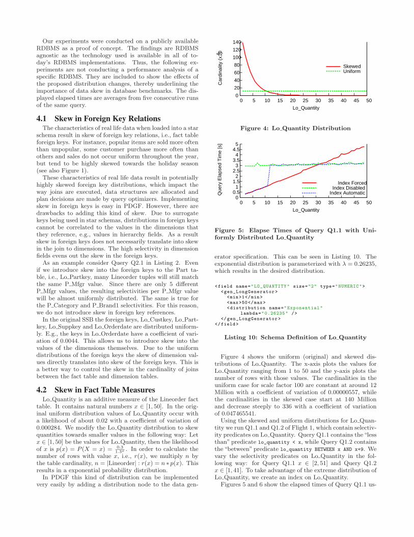
Figure 4 shows the uniform (original) and skewed dis-tributions of Lo Quantity. The x-axis plots the values forLo Quantity ranging from 1 to 50 and the y-axis plots thenumber of rows with those values. The cardinalities in theuniform case for scale factor 100 are constant at around 12Million with a coefficient of variation of 0.00000557, whilethe cardinalities in the skewed case start at 140 Millionand decrease steeply to 336 with a coefficient of variationof 0.047465541.

Using the skewed and uniform distributions for Lo Quan-tity we run Q1.1 and Q1.2 of Flight 1, which contain selectiv-ity predicates on Lo Quantity. Query Q1.1 contains the“lessthan” predicate lo_quantity < x, while Query Q1.2 containsthe “between” predicate lo_quantity BETWEEN x AND x+9. Wevary the selectivity predicates on Lo Quantity in the fol-lowing way: for Query Q1.1 x ∈ [2, 51] and Query Q1.2x ∈ [1, 41]. To take advantage of the extreme distribution ofLo Quantity, we create an index on Lo Quantity.

Figures 5 and 6 show the elapsed times of Query Q1.1 us-

1 1.5

2 2.5

3 3.5

4 4.5

5 5.5

6

0 5 10 15 20 25 30 35 40 45 50

Que

ry E

laps

ed T

ime

[s]

Lo_Quantity


Index Automatic

Figure 6: Elapse Times of Query Q1.1 with SkewedDistributed Lo Quantity

ing the three modes explained above and varying the predi-cate lo_quantity < x, x ∈ [2, 51] on both the uniform andskewed data sets. The solid line in Figure 5 shows theelapsed times of index driven queries. The elapsed timesincrease linearly with increased values of Lo quantity. Itstarts with about 0.4s at x = 2 and increases linearly to 4.8sat x = 51. This is not surprising as the advantage of theindex diminishes with increased values for x, i.e., the num-ber of rows qualifying for the index driven join increases-linearly with increased values of x. The dashed line showsthe elapsed time of the non-index driven join queries. Thisline is flat at about 3s. This is also not surprising as the non-index driven join queries have to scan the entire Lineordertable regardless of substitution parameters. That is, the in-dex driven queries outperform the non-index driven queriesuntil x = 31. The dotted line shows the elapsed time ofqueries when the query optimizer is free to choose the bestexecution plan. This line shows that the query optimizerswitches from an index driven join to an non-index drivenjoin at x = 12. This is suboptimal as the real cutoff of indexdriven joins is at about x = 31. That is the query optimizerswitches too early from an index driven join to a non-indexdriven join.Figure 6 repeats the same experiments on skewed data.

As in the uniform case the elapsed times of the index drivenqueries, as indicated by the solid line, and the elapsed timesof the non-index driven queries, as indicated by the dashedline follow the skewed Lo Quantity distribution. Due to theextreme skew in Lo Quantity, the index driven queries out-perform the non-index driven queries only for values x < 5.The dotted line shows the elapsed time of queries when thequery optimizer is free to choose the best execution plan.It shows that the optimizer switches from an index drivenplan to a non-index driven plan at the same value for x asin the uniform experiment, namely at x = 11. However, thisswitch is suboptimal. It should have occurred earlier, i.e.,at x = 5.These experiments show that the optimizer factors the

selectivity of certain predicates in the query planning. How-ever, the fact that the switch in the query plan from in-dex driven to non-index driven occurs at the same predicateparameter for skewed and uniform data suggests that theoptimizer does not consider the data distribution for thisdecision.Figures 7 and 8 show the elapsed times of Query Q1.2

on uniform and skewed data in the above described three

1.2 1.4 1.6 1.8 2

2.2 2.4 2.6 2.8 3

0 5 10 15 20 25 30 35 40

Que

ry E

laps

ed T

ime

[s]

Lower Range for Lo_Quantity Range

Index forcedIndex disabled

Index automatic

Figure 7: Effect of skewed Lo Quantity on QueryQ1.2 elapsed times

0.5 1

1.5 2

2.5 3

3.5 4

4.5 5

5.5 6

0 5 10 15 20 25 30 35 40

Que

ry E

laps

ed T

ime

[s]

Lower Bound for Lo_Quantity Range

Index forcedIndex disabled

Index automatic

Figure 8: Effect of skewed Lo Quantity on QueryQ1.2 elapsed times

optimizer modes. Similarly, as in the experiments for QueryQ1.1, we vary x ∈ [1, 41] in lo_quantity between x and x+9.

Figure 7 shows that the elapsed times of Query Q1.2 stayconstant for each of the three modes regardless of the sub-stitution parameter x. On average the index driven queriesexecute in 2.63s with a coefficient of variation of 0.024, whilethe non-index driven queries and the queries chosen in theautomatic mode execute on average in 1.42s with a coeffi-cient of variation of 0.021. The index driven queries outper-form the non-index driven queries by 46% and the lines forindex forced and index automatic overlap.

Figure 8 shows that in the skewed case Query Q1.2 ben-efits from non-index driven joins in cases of high selectivity.The elapsed times of the non-index driven queries are ag-nostic to the substitution parameter x. With an average of2.69s at a coefficient of variation of 0.038, which is similar tothe uniform case, they outperform the index driven queriesfor x < 10. The index driven queries follow the distribu-tion for Lo quantity (see Figure 4), i.e., they monotonouslydecrease with increasing x. For x >= 10 the index drivenqueries outperform the non-index driven queries. The lineshowing the elapsed times of queries in the automatic modeindicates that the system makes the right choice switchingfrom non-index driven queries to index driven queries atx = 10.

4.3 Skew in Single Dimension HierarchiesSelectivity in many of the original SSB queries is con-

trolled by predicates on hierarchy columns. Each dimen-sion table defines one three-column hierarchy. Each col-umn of a hierarchy defines a different range of values. Col-umn cardinality increases as individual queries of flights

0

10

20

30

40

50

60

70

55 44 33 23 31 11

Car

dina

lity

(x104 )

Category Number

SkewedUniform

Figure 9: P Category Distribution Uniform andSkewed

drill down into hierarchies. For example, the Part tabledefines the following hierarchy: P Brand → P Category →P Mfgr. Values for these hierarchy columns are generatedin the following way: Values in P Mfgr are used as pre-fixes in P Category whose values again serve as prefixes inP Brand. While P Mfgr contains five different values m ∈{MFGR#1, ...,MFGR#5}, P Category contains 25 differ-ent values c ∈ {MFGR#11, ...,MFGR#55} and P Brandcontains 1000 values b ∈ {MFGR#1101, ...,MFGR#5540}.By varying the projection predicates in queries for thesethree columns, the join selectivity can be varied as well.Consider Query Q2.1 in Listing 2; due to the hierarchy andthe uniform distributions in all values and references onecan easily see that the selectivity on Part and thus also onLineorder is 1

5of the size of the tables. By changing the

restriction to Category, e.g., p_category = ’MFGR#22’, the joinselectivity can be reduced to 1

25. The set ratio between the

number of rows qualifying a specific substitution parameteris exploited in the query flights.By introducing skew in these columns the above property

may be lost. However, if we control the skew and are ableto estimate the frequency of each value, the selectivity cal-culations are still possible. Therefore, we set a predefinedprobability for each value in the part hierarchy. For thenumbers in Mfgr and Category we use the following prob-abilities: 1 70%, 2 20%, 3 6%, 4 3%, and 5 1%. For in-stance, the value “Mfgr#1” appears with a probability of70% and the category “Mfgr#11” occurs with a probabilityof 70% ∗ 70% = 49%. The values where chosen to have onerange that has the same probability as in the uniform case(i.e., “MFGR#2” and “MFGR#22”). This makes it possibleto specify queries with the same selectivity for the skewedand uniform data. SSB Query Q1.3 includes a range selec-tion on Brand1. Therefore, we define ranges with the sameprobability in column Brand1. The selectivities in Brand1are: 1-10 70%, 11-20 25%, 21-30 4.5%, and 31-40 0.5%. Thusbrands in the range of “MFRG#2211”-“MFRG#2220” havethe same probability as in the uniform case.Figure 9 displays the uniform and skewed distribution of

values in the P Category column. The cardinalities of theuniform distribution stay at around 4% with a coefficient ofvariation of 0.0044. The cardinalities in the skewed distri-bution vary between 0.01% and 48.36% with a coefficient ofvariation of 2.5028.Skew in P Category can be implemented in PDGF as de-

scribed in Listing 11. It shows the definition of the P Mfgrfield. Each value consists of two parts, the prefix “MFGR#”

4 4.5 5

5.5 6

6.5 7

7.5 8

8.5 9

55 44 33 23 31 11

Que

ry E

laps

ed T

ime

[s]

Category Number


Index Automatic

Figure 10: Elapsed Times of Query Q2.1 with Uni-formly Distributed P Category

0

5

10

15

20

25

55 44 33 23 31 11Q

uery

Ela

psed

Tim

e [s

]Category Number


Index Automatic

Figure 11: Elapsed Times of Query Q2.1 withSkewed Distributed P Category

and a number between one and five. The probability for eachnumber is explicitly defined as specified above. The defini-tion of the fields P Category and P Brand1 is implementedin the same way, by explicitly giving the probabilities.

<field name="P_MFGR" size="6" type="VARCHAR"><gen_PrePostfixGenerator><gen_ProbabilityGenerator><probability value="0.70"><gen_StaticValueGenerator><value>1</value>

</gen_StaticValueGenerator></probability ><probability value="0.20"><gen_StaticValueGenerator><value>2</value>

</gen_StaticValueGenerator></probability >[..]

</gen_ProbabilityGenerator><prefix>MFGR#</prefix>

</gen_PrePostfixGenerator></field>

Listing 11: Definition of Skew in P Mfgr Field

Query Q2.1, as defined in Listing 2, can be used to demon-strate the effects of the skewed distribution on query execu-tion times. In Figure 10, the execution times of all pos-sible values of P Category are shown for the uniform, i.e.,original distribution, and in Figure 11, they are shown forthe skewed distribution. As can be seen in the graph, theexecution times for the queries in the uniform case are al-most constant as expected, because the query predicate isan “equal” predicate in Q2.1. Interestingly, the query op-

timizer consistently chooses the wrong query plan, i.e., anindex-driven plan. In the skewed case, the execution timesare increasing with the selectivity for the index driven queryplan and constant for the plan without index. As in previ-ous experiments, the query optimizer is aware of the skewin the selectivity of P Category as can be seen at the auto-matic plan in the skewed case. However, the query optimizerswitches from an index to non-index plan too early, thus sig-nificantly increasing the query elapsed time. This behaviorcan only be observed on the skewed data set. With the regu-lar data set the source of the less efficient query plan cannotbe determined.

4.4 Skew in Multiple Dimension HierarchiesThis section discusses the introduction of data skew in

multiple dimensions and its effect on query elapsed times.Similar to the data skew in the P Brand1 → P Category →P Mfgr hierarchy of the Part table, data skew can be imple-mented in the City → Nation → Region hierarchies of theSupplier and Customer tables. Having five regions in eachtable (Supplier, Customer) results in a selectivity of 1

5in the

uniform case. Each region contains 5 nations, each with aselectivity of 1

25. Each nation contains 10 cities for a total se-

lectivity of 1250

. Queries in flights 3 and 4 compare customerwith supplier using various levels in the above hierarchies.For our experiments, we modify S City and C City to

follow an exponential distribution. For simplicity, we as-sign each city of the Supplier and Customer tables a uniquenumber: cs ∈ [1, 250] for Supplier and cc ∈ [1, 250] forCustomer. The likelihoods of Supplier and Customer citiesare then defined as p(cs) = P (C = cs) = 0.0309

1.0309csand

p(cc) = P (C = cc) = 0.041.04cc

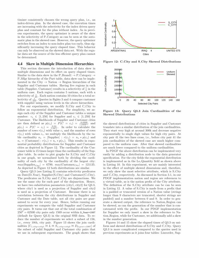
. In order to calculate thenumber of rows r(cs) with value cs and the number of rowsr(cc) with values cc, we multiply the likelihoods by the ta-ble cardinality ns = |Supplier| : r(cs) = ns ∗ p(cs) andnc = |Customer| : r(cc) = nc ∗ p(cc). This results in expo-nential probability distributions for Supplier and Customercities as depicted in Figure 12. The cardinality of the Cus-tomer table is 15 times larger than the cardinality of the Sup-plier table. In order to plot graphs for S City and C Cityin one graph, we normalized both by dividing the cardi-nality of each city by the cardinality of the largest city:max|SupplierCity| = 6799, max|CustomerCity| = 121135.As depicted in Figure 12 both distributions are similar.Query Q3.3 (see Listing 3) contains selectivity predicates

on Date(D Year), Supplier(S City) and Customer(C City).The predicates on S City and C City are disjunctions. Weuse the same city for each part of the disjunction. Hence,we have two substitution parameters (city1, city2) for Q3.3,where city1 is used as a projection of Supplier and city2is used as a projection of Customer. Because there is nocorrelation between the city distributions in Supplier andCustomer and the Date table, not all city pairs are guar-anteed to occur for every year. Hence, before running ourexperiments we compute the valid Supplier and Customercity pairs. It turns out that out of the total combination of2502 = 62500 city pairs only 1569 occur within D_Year=1997

(default for Query Q3.3) in the original SSB data. To re-duce the number of experiments we select a subset of 156,i.e., every 10th, city pair. Figure 13 shows the join cardi-nalities |Cc city=city1 ✶ L ✶ Ss city=city2 ✶ Dd year=1997| ofthe subset of valid Supplier and Customer city pairs thatwe use in subsequent experiments. The graph shows that

0

0.2

0.4

0.6

0.8

1

ARGENTINA1 IRAQ 4 UNITED ST5

Nor

mal

ized

Car

dina

lity

Cities

S_CITYC_CITY

Figure 12: C City and S City Skewed Distributions

0

50000

100000

150000

200000

250000

300000

350000

0 20 40 60 80 100 120 140 160

Join

Car

dina

lity

Selected City Pairs

UniformSkewed

Figure 13: Query Q3.3 Join Cardinalities of theSkewed Distributions

the skewed distributions of cities in Supplier and Customertranslate into a similar distribution of the join cardinalities.They start very high at around 300k and decrease negativeexponentially to single digit values for high city pairs. Atcity pair 41 the two lines cross, i.e., before city pair 41 thejoin cardinalities of the skewed case are much higher com-pared to the uniform case. After that skewed cardinalitiesare much lower compared to the uniform cardinalities.

In PDGF the above distribution can be implemented veryeasily by adding a distribution node to the data generatorspecification. For the city fields the exponential distributionis implemented as in the Lo Quantity field as shown abovein Listing 10. In this experiment, we are mainly interestedin the effect of multiple skewed dimensions and, therefore,we only skew the most selective attribute, which is S Cityand C City, respectively. As discussed in Section 3.1, in ourPDGF implementation nation and region are references toa virtual table, as is the nation prefix of the City attribute.The definition of the S City attribute can be can be seenin Listing 12. A value of S City is made from a prefix thatis a padded or truncated version of a Nation value (stringslonger than 9 characters are truncated, shorter strings arepadded) and a number between 0 and 9. In order to gen-erate a skewed output, the reference to Nation Region canbe skewed, as can the generation of the number that is con-catenated with the prefix. In our PDGF implementationfor Supplier we only insert a skew in the reference to Na-tion Region, while for Customer, we additionally add a skewin the number generation.

Figures 14 and 15 show the elapsed times of Q3.3 on uni-form and skewed distributions of S City and C City. QueryQ3.3 is more complicated compared to the queries used inprevious experiments as it joins four tables: Lineorder, Sup-

0

1

2

3

4

5

6

7

8

0 20 40 60 80 100 120 140 160

Que

ry E

laps

ed T

ime

[s]

Selected City Pairs


Index Automatic

Figure 14: Elapsed Times of Query Q3.3 with Uni-form C City and S City

<field name="S_CITY" size="10" type="VARCHAR"><gen_SequentialGenerator concatenateResults="true">

<gen_PaddingGenerator ><gen_DefaultReferenceGenerator id="S_CITY_id">

<reference table="NATION -REGION"field="NATION" />

</gen_DefaultReferenceGenerator><character > </character ><padToLeft >false</padToLeft ><size>9</size>

</gen_PaddingGenerator ><gen_LongGenerator>

<min>0</min><max>9</max>

</gen_LongGenerator></gen_SequentialGenerator>

</field>

Listing 12: Definition of S City in the Supplier table

plier, Customer and Date. Due to the increased complex-ity, the choices for indexes and query plans for Query Q3.3.are much larger compared to those in previous experiments.Hence, the index driven join forces the system to use a queryplan that does not necessarily coincides with the query planchosen by the optimizer in automatic mode.Figure 14 shows the elapsed times for all three modes on a

uniform data set. Each line shows a constant query elapsedtime regardless of the city pair chosen. This is not surprisingas the cardinalities of at which each city pair occurs in thedatabase is constant (see Figure 12. The non-index drivenqueries have the longest elapsed times while the automaticqueries have the shortest elapsed times. The index forcedqueries execute slightly longer than the index driven queries.Figure 15 shows the elapsed times for all three modes on

the skewed data set. The graph reveals a couple of veryinteresting characteristics of the system. The elapsed timesof the non-index driven queries, dashed line, is more or lessconstant at about 7s. Queries using the first 20 city pairs,which result in very high join cardinalities (50k to 300k)show slightly higher elapsed times (up to 9s). This is dueto the larger intermediate result set at these high join cardi-nalities. Contrary, the lines for index forced and index au-tomatic plans show a steep decrease in elapsed time startingat city pair 30 for the automatic plan and 34 for the indexforced plan. The steep decrease is due to the steep decreasein the join cardinality. That is the index driven queries areable to take advantage of the index to filter out most ofthe rows to beat the non-index driven queries. Again, thisis due to a sub-optimal query plan that was forced in the

0

2

4

6

8

10

12

14

0 20 40 60 80 100 120 140 160

Que

ry E

laps

ed T

ime

[s]

Selected City Pairs


Index Automatic

Figure 15: Elapsed Times of Query Q3.3 withSkewed C City and S City

0

1

2

3

4

5

6

7

8

0 20 40 60 80 100 120 140 160Q

uery

Ela

psed

Tim

e [s

]Selected City Pairs

Automatic UniformAutomatic Skewed

Figure 16: Elapsed Times of Query Q3.3 with Uni-form and Skewed C City and S City using Auto-matic Plans

index-forced mode. Also, like in the uniform case, the au-tomatic query outperforms both the index driven and non-index driven queries for all city pairs.

Figure 16 compares the automatic case for the uniformand skewed distributions. The queries run on uniform dataexecute constantly under 1s, while the queries on skeweddata follow the cardinality distribution as described above.With a decrease in join cardinality the queries on skeweddata outperform those on uniform data, which is not sur-prising. However, the cross over point seems to be at citypair 52. We would have expected the cross over to be closerto city pair 41, where the join cardinalities of the skewed anduniform data sets are identical. This shows that the systemhas a consistently increased latency for skewed data. Thistrend also holds for the index-forced and no-index plans.

5. RELATED WORKWhile the importance of data skew in database processing

has been identified and, to some degree, quantified in var-ious publications, especially in the field of parallel systems[8, 16], there is no industry standard benchmark that mea-sures the effect of data skew on query processing. In manycases, performance of parallel DBMS is adversely affected bydata skew, because it introduces load imbalances, stressesthe creation of internal data structures, and it reveals poordesign decisions in algorithms and query optimizers. Havingrealized the above, Crolotte and Ghazal proposed the intro-duction of data skew into TPC-H similarly to TPC-DS, i.e.,using comparability zones [5]. As a consequence, queries are

still run with substitution parameters that are chosen fromwithin a comparability zone with uniform distribution.[5] discusses two approached how skew can be introduced

into the nation keys of the Customer and Supplier tables.The first approach scales the numbers of customers andsuppliers who reside in a nation proportional to the actualpopulation of this nation (e.g., obtained from the US cen-sus). Although being realistic this approach is not feasible inthe context of TPC-H as the queries would impose differentworkloads for different customers. Their second approach,which is feasible for TPC-H is creating skew with a step func-tion. The first 13 nations have a small population, while theremaining 12 nations have a large population. They imple-ment the above described skew using Teradata SQL syntaxwith a random function, i.e., they read the original TPC-Hdata and apply a random function for nation keys.Closer to our approach for introducing data skew in stan-

dard benchmarks is Chaudhuri and Narayasa modified ver-sion of TPC-D [3]. TPC-D was the precursor of TPC-H. Thetwo benchmarks share the same schema and data model, butvary in their workload slightly. Hence, the proposed changesalso apply to TPC-H. Chaudhuri and Narayasa modifiedTPC-D/H’s data generator dbgen to support Zipfian dis-tributed data in all columns. The parameter to the distri-bution (ρ), which controls the degree of skew in the data,is given as a parameter to the modified version of dbgen. ρ

can be set to any value larger or equal to 0; ρ = 0 generatesa uniform data whereas ρ = 4 generates a highly-skeweddistribution. In addition they also implemented functional-ity that allows dbgen to randomly chose ρ values for eachcolumn, thereby creating a “mixed” data distribution.Their approach differs from Crolotte and Ghazal’s ap-

proach as it does not guarantee workload predictability, whichis a major factor in industry standard benchmarks and inparticular in TPC-H. However, Chaudhuri and Narayasa ap-proach can be easier implemented as the data generator isfreely available, but it is limited to the Zipf distribution andcannot be customized on a column per column basis.Data skew has been addressed to some extend in TPC-

DS. The TPC after realizing that the uniform data distribu-tions in TPC-D, TPC-H and TPC-R were not challengingtoday’s DBMS vouched to implement data skew in its nextdecision support benchmark TPC-DS. The TPC opted fora solution that introduced zones of comparability – essen-tially flat spots in the data distribution – that can be used toprovide both the variability and the comparability that theeventual user of the generated data requires. These compa-rability zones differ in size within the column domain andin number between column domains.

6. CONCLUSIONIn this paper, we presented an extension of the Star Schema

Benchmark that introduces skew in single table columns andsingle table hierarchies. Due to the limited extensibility ofthe original data generator, we implemented a new datagenerator and query generator based on the Parallel DataGeneration Framework. Our extensive experimental analy-sis shows that the introduction of skew in the data sets canuncover unpredicted behavior in query processing.PDGF is continuously extended and improved. A recent

extension was presented in [6]. It allows for the efficientgeneration of consistent update data. This enables PDGFto generate more realistic updates on the data compared to

TPC-H and SSB. However, we did not explore this optionin the presented work. Information on the current statusof PDGF as well as downloadable versions can be found onwww.paralleldatageneration.org.

For future work, we will explore the possibilities of us-ing references to the generated data set in query generation.This will make it possible to introduce skew in the queryworkload and thus make it possible to examine the influ-ence of query caching and other optimizations in a mean-ingful way. In combination with the deterministic data gen-eration the reference-based query generation will enable pre-computation of query results for certain kinds of queries andthus provide means for verification beyond the capabilities ofcurrent benchmarks. We will combine these and the abovepresented parts into a complete benchmark suite that willmake it possible to test the different influences of skew inseparated and combined workloads.

7. REFERENCES[1] TPC Benchmark H.

http://www.tpc.org/tpch/spec/tpch2.15.0.pdf, 2012.

[2] J. S. Charles Levine. Standard Benchmarks for DatabaseSystems. http://www.tpc.org/information/sessions/sigmod/sigmod97.ppt, 1997.

[3] S. Chaudhuri and V. Narasayya. Program for GeneratingSkewed Data Distributions for TPC-D. ftp://ftp.research.microsoft.com/users/viveknar/tpcdskew, 1997.

[4] E. F. Codd. A Relational Model of Data for Large SharedData Banks. Communications of the ACM, 13(1):377–387,1970.

[5] A. Crolotte and A. Ghazal. Introducing Skew into theTPC-H Benchmark. In TPCTC ’11, pages 137–145, 2011.

[6] M. Frank, M. Poess, and T. Rabl. Efficient Update DataGeneration for DBMS Benchmark. In ICPE ’12, 2012.

[7] R. Kimball and M. Ross. The Data Warehouse Toolkit:The Complete Guide to Dimensional Modeling. John Wileyand Sons, Inc., 2002.

[8] M. S. Lakshmi and P. S. Yu. Effect of Skew on JoinPerformance in Parallel Architectures. In DPDS, pages107–120, 1988.

[9] G. Marsaglia. Xorshift RNGs. Journal Of StatisticalSoftware, 8(14):1–6, 2003.

[10] R. O. Nambiar and M. Poess. The Making of TPC-DS. InVLDB ’06, pages 1049–1058, 2006.

[11] P. O’Neil, E. O’Neil, X. Chen, and S. Revilak. The StarSchema Benchmark and Augmented Fact Table Indexing.In TPCTC ’09, pages 237–252, 2009.

[12] M. Poess and C. Floyd. New TPC Benchmarks for DecisionSupport and Web Commerce. SIGMOD Record,29(2000):64–71, 2000.

[13] M. Poess, T. Rabl, M. Frank, and M. Danisch. A PDGFImplementation for TPC-H. In TPCTC, pages 196–212,2011.

[14] M. Poess and J. M. Stephens. Generating ThousandBenchmark Queries in Seconds. In VLDB, pages1045–1053, 2004.

[15] T. Rabl, M. Frank, H. M. Sergieh, and H. Kosch. A DataGenerator for Cloud-Scale Benchmarking. In TPCTC ’10,pages 41–56, 2010.

[16] C. B. Walton, A. G. Dale, and R. M. Jenevein. ATaxonomy and Performance Model of Data Skew Effects inParallel Joins. In G. M. Lohman, A. Sernadas, andR. Camps, editors, VLDB ’91, pages 537–548. MorganKaufmann, 1991.

variations of the star schema benchmark to test the

Documents