vdm aggregation strategy - infokarta.com stragtegy - white paper...vdm aggregation strategy ......

[email protected] 1 © InfoKarta Inc. 2015

VDM Aggregation Strategy

By Michael Kamfonas

A successful performance strategy for very large databases (VLDB) often involves

aggregations. This is why major DBMS vendors offer mature system support for

aggregation maintenance and optimization. DB2 offers Materialized Query Tables

(MQT), Teradata offers Aggregate Join Indexes (AJI), Oracle offers Materialized Views

(MV). BI tool vendors support aggregate awareness and dynamic sourcing, while OLAP

technologies offer cost-effective, in-memory retention alternatives. All too often, however,

these powerful capabilities are used redundantly, without too much forethought, and

although they often improve query performance, they sometimes also disappoint, by

impacting ETL windows, availability, stability, sustainability and sometimes quality. This

is an overview of InfoKarta’s approach to implementing an Aggregation Strategy. It

proposes a model and a framework to reason about aggregates, qualify work-loads that

benefit from them, and pick most effective levels from a total performance perspective. It

also recommends design and implementation approaches for exploiting the DBMS

aggregation technology at hand in a way that is resilient, sustainable, scalable and

maintainable. The techniques described are part of the Versioned Dimensional Model1

(VDM) Toolkit and methodology which originated in the early 90s by the author, and has

been evolving ever since.

Why an Aggregation Strategy?

The conversation usually goes something like this:

Me: We need to optimize for Sales Dashboard queries at any level of Location, Product

and Time Period. We should be able to support minimum service levels across the

envelope of all drill-down summaries that these queries can hit.

DBA: Even very similar queries may follow different execution plans. We need to

optimize for the levels and types that are most critical. Let’s get a list of the 10-20

typical or worst offender queries to optimize. Then we will clearly be able to

measure success and know when we are done. Then we can repeat the exercise.

Me: Even if we pick 20 queries, we know that the patterns will change or new ones will

emerge. We need to ensure that the whole envelope of dashboard queries has good

response. All these queries are one or two-level drilldowns, and must consume less

than 150 CPU-seconds average to sustain the required concurrency. At the same

1 The Versioned Dimensional Model (VDM) comprises methods and techniques around the design and

implementation of analytic and reporting databases, bridging the gap between operational and dimensional

models with emphasis on performance on parallel share nothing platforms. The VDM-Toolkit© is a

framework of customizable tools and accelerators around the author’s VDM practice.

mailto:[email protected]


time we have to make sure that heavily hit levels are supported with close enough

aggregates to reduce total cost.

DBA: This is too open-ended. Query patterns are too nebulous. We cannot optimize for

queries we can’t see or run. I say, find the most common queries and optimize for

those. We can continue monitoring the workload, find new worst offenders the

following week and optimize them in the next round. Iterative improvement is the

name of the game!

This article was conceived to articulate how optimizing for aggregation envelopes and

query patterns can be conceived, approached systematically, measured and architected.

If this thought appeals to you, or any of the situations below sound familiar, you should

read-on:

Overnight maintenance windows get tighter and tighter. Opening times start getting

missed as more and more aggregations elongate ETL cycles and squeezing

contingency margins.

Unexpected delays of alarming magnitude started to occur occasionally.

Aggregation maintenance can add unpredictability to ETL time windows. Small

dimension changes, for example, can cause disproportionately large and expensive

updates when recasting is involved.

Inconsistencies between base and aggregates cast doubt in users’ mind about the

quality of data. Missed or delayed maintenance causes discrepancies to become

visible through reports or dashboards. Adding insult to injury, it is often the users

that discover these issues and tracing the root cause can be time-consuming and

sometimes inconclusive.

Newly introduced reports or query patterns, with no aggregate support, abuse

resources saturating the system and impacting other production workloads. Existing

aggregate JIs or MQTs need to be adjusted or new ones introduced.

After two years of active use, it is not uncommon for a data warehouse to lose a

third or more of its capacity in redundant or unnecessary copies of data. As

migrations to newer versions of base or derived data occur, some applications

remain coupled to older, now redundant, data objects. Application change is

required, hampering the elimination of old data which as time goes by and the focus

of key developers moves to other areas it becomes riskier to do. Inevitably, the only

viable solution is to upgrade capacity earlier than planned. The reasons for data

redundancy are many, and aggregate-to-application coupling is one of them.

OLAP and in-memory cube technologies reduce the costs of high concurrent usage

and can be welcome additions to our arsenal. But how does one prevent rules and

metric definitions from drifting into inconsistent parochial application meta-models

and enforce consistency across all access tools in the data warehouse environment?



The Problem Space

Data warehouses, data marts and BI tools enable a chain of model transformations that

start from the source normalized model, and end in the myriad of result sets delivered to

end-applications and users. The architect has to decide which “snapshots” of this

transformation chain to instantiate into concrete materialized physical objects, effectively

dividing the chain into daily batch and on demand segments. Figure 1 shows this

continuum and how the options explode as we move away from the source model and

towards the right, the consumption-end of the warehouse. The most popular choice is to

materialize a base model close to the source model. This not only favors ETL simplicity

but it also preserves, relatively untampered, the original content satisfying the broadest

spectrum of requirements either not yet uncovered or needing correction or

reinterpretation. Downstream transformation from the base model ideally could be

dynamic, through one or more layers of views, delivering an access layer organized by

functional area of interest. This access layer often presents a dimensional model that

makes it easy for applications and users not only to select and filter, but also to aggregate

and combine facts to derive complex metrics. Keeping this transformation dynamic is

elegant, maximizes availability and keeps the pain of change low since the base model is

relatively normalized. However, even with ideal indexing and physical organization,

there is too much transformation left in the pipeline to absorb at query time, leading to

performance degradation, saturation of resources and excessive cost.

Sources Base Model Aggregates

ReportsQueries

Query time cost

Aggregate maintenance cost

ETL cost

Figure 1 Transformation pipeline and choice of materialization points



To mitigate the problem we seek appropriate intermediate materialization points along

the transformation path to take some of this burden away from the query, process it in

advance, typically once a day, and share it across multiple more efficient query

executions. The improvement most typically comes by reducing I/O in the form of pre-

joins and aggregations. The further to the right of the diagram these aggregates fall i.e.

the closer to the targeted reports, the more efficient queries will become; but also the

more explosive the encountered patterns, and thus the cost of aggregate maintenance. The

VDM Aggregation Strategy is a methodology that finds and implements aggregates to

optimize holistic system performance. It is appropriate where a large portion of the query

workload aggregates data and follows a dimensional pattern, even if the schema is not

dimensional.

The essence behind a dimensional query pattern is in the aggregation of lower level

events along the apparently independent (but potentially correlated) classifiers and

taxonomies they are joined with. The schema best suited for this purpose is highly

dependent on the DBMS support in terms of optimization capability and implemented

access methods. Typically, the CPU and I/O costs are highly correlated to the number of

rows scanned. Our optimization approach seeks to minimize row counts by pre-

aggregating data, while also combining other pragmatic considerations to arrive at a

rational, flexible solution.

The three obvious questions, when it comes to aggregations, are:

What are the optimal levels?

How should we implement and maintain them?

How can we exploit them so our queries run predictably faster?

In support of the last two bullets, major DBMSs (DB2, Teradata and Oracle) offer

methods for defining and maintaining aggregates automatically, and provide some type of

re-write capability during optimization to redirect qualifying queries to the appropriate

aggregate. There are nuances in the implementations and each DBMS vendor puts forth

good reasons on why they do or don’t allow certain features. For example, Teradata only

allows system-maintained Aggregate Join Indexes (AJIs) keeping the implementation

simpler and always ensuring consistency between base tables and aggregate. IBM/UDB

and Oracle allow more flexibility, adding options for deferred or user-maintained MQTs

and MVs. This flexibility comes at the cost of more complexity and risk exposure. Of

course, good old-fashioned aggregate tables with no DBMS support are always available

and OLAP, in-memory cube technologies or BI-tool capabilities add to the menu of

choices.

The successful aggregation strategy is less about features, and more about how well we

exploit the capabilities available to us. The approach described below combines

analytical optimization techniques with technology-specific practices, and pragmatic

considerations for complexity, stability and sustainability.



The VDM Aggregation Strategy Framework

The “Aggregation Lattice”

We use two types of graphic representations to aid us in visualizing aggregations. The

“Level Grid” illustrated in Figure 2 shows a fact (in green) with additive metrics M1, M2,

against the five dimension keys D1-D5. The dimensions are represented by vertical lines

stemming off these keys with their levels numbered starting from zero.

D1 D2 D3 D4 D5 M1 M2

0

1

2

3

4

Figure 2 - Basic Dimensionality of our example fact

The black line at the bottom denotes the base level of the fact, while the blue line at

(2,4,3,3,3) indicates the top aggregate along all dimensions – a single row summary. Any

line which cuts across the five dimensions at a valid level represents an aggregation. The

red one shown in the Figure 2 is at level (1,1,2,2,0).

The “Aggregation Lattice” is the second type of graph we use, depicting all possible

aggregations from the base fact to the highest level. Every aggregation-defining line that

cuts across our “level Grid” corresponds to a node of the Aggregation Lattice. The lattice

also has edges that indicate all possible derivation paths of each aggregate from lower

levels. Our example in figure 1 has 3x5x4x4x4=960 possible such lines of dimension

level combinations or 960 nodes in the corresponding Aggregation Lattice. Since such

size lattice would be too cluttered to work and visualize, Figures 3 and 4 show smaller

examples with two and three dimensions respectively. Here are the conventions we use to

construct these lattices:



1. Each dimension is a tree of uniform depth, with its nodes organized in levels, with a

single top node representing “all” or “any”. Leaf nodes are at level 0; their parents are

at level 1; their parents at level 2 etc. The root (top) node level is 1n , where n

represents the number of levels in the dimension. Simple codes with no hierarchical

structure can be represented in two levels: the code itself at level-0, and a single

parent denoting the “any code” at level 1.

2. There are as many possible aggregates as there are combinations of participating

dimension levels. We use the term “multi-levels” when we want to distinguish them

from single dimension levels. A bottom multi-level for a three-dimensional model is

(0,0,0)2 and it represents the base fact; the top can be something like (4,5,4)

representing all stores, all product, for all time. All possible multi-levels between top

and bottom are connected by arcs depicting every possible single-dimension single-

level aggregation path. The graph so formed is a lattice, “the Aggregation Lattice,” a

complete map of all valid aggregation paths.

Three lattice examples of a two-dimensional hierarchy are depicted in Figure 3. The

number of nodes (vertices for the mathematically inclined) is the product of the number

of levels for each dimension; from left to right, 2x2 = 4, 4x4 = 16 and 3x3 = 9. Similarly,

Figure 4 depicts three-dimensional lattices for two and three level hierarchies with 2x2x2

= 8 and 3x3x3 = 27 nodes respectively. For illustration purposes we show transitive

aggregations using dashed lines for the 3x3 lattice.

(0,0)

(1,1)

(0,1)(1,0)

(2,2)

(0,0)

(1,1)

(0,1)(1,0)

(1,2)

(0,2)(2,0)

(2,1)

(3,3)

(0,0)

(1,1)

(0,1)(1,0)

(1,2)

(0,2)(2,0)

(2,1) (0,3)(3,0)

(2,2) (1,3)(3,1)

(2,3)(3,2)

Figure 3: Two-dimensional aggregation lattices 2, 3 and 4 levels deep.

2 There is a subtle difference between the base fact (0,0,0) and the transactional detail level, where all event

data are stored. The methodology uses an additional node, referred to as level -1 below the (0,0,0) level to

denote the non-aggregated underlying event data. For simplicity, we ignore it during this discourse.



There is more than one way to derive an aggregation from lower levels, and the number

of ways increases as the number of dimensions increase. For example, (2,0,2) is derived

by aggregating one level along the third dimension of (2,0,1) or along the first dimension

of (1,0,2), or by aggregating any of the lower levels, i.e. (2,0,0), (1,0,1), (0,0,2) or (1,0,0),

(0,0,1) and (0,0,0).

In the diagrams we show vertices in layers, each representing multi-levels of the same

“rank” or “aggregation distance” from the bottom. The lowest, single vertex represents

the base fact and has rank 0; the next layer-up has vertices with rank 1, and so on. The

rank correlates to the “level of magnitude” of an aggregate in terms of row count. To

illustrate this, visualize an ideal mart where all dimensions are independent with same

depth and cardinality ratio 10:1 from level to level. If the base fact has 1 million rows the

vertices in the next layer represent multi-levels (or aggregates) with rank 1 and 100,000

rows. The next layer of rank 2 will have cardinalities ten times less and so on. Of course

in reality dimensions are not independent and cardinality ratios vary. This causes

aggregates of the same rank to have very different row-counts. This is why we use the

notion of “rank” to talk about the topology, but we compute actual cardinalities to

analyze performance potential.

(0,0,0)

(1,1,1)

(0,1,0)(1,0,0)

(2,2,2)

(0,0,0)

(1,1,0)

(0,0,1)(1,0,0)

(0,1,2)

(0,0,2)(2,0,0)

(2,1,0)

(0,0,1)

(0,1,0)

(1,0,1)(0,1,1)(0,2,0)

(2,0,1) (1,0,2)(1,1,1)(1,2,0) (0,2,1)

(2,1,1) (0,2,2)(2,2,0) (1,2,1)(1,1,2)(2,0,2)

(1,2,2)(2,2,1) (2,1,2)

(1,0,1)(1,1,0) (0,1,1)

Figure 4 Tree-dimensional aggregation lattice 2 and 3 levels deep.

The first step of our process is to form a “Loaded, Weighed Aggregation Lattice” as

follows:



1. Establish the dimensionality of each fact. This is a critical step, particularly if the

underlying schema is non-dimensional. This entails organizing the model into

dimensions, picking the relevant levels and pruning those dimensions that we

should not consider or that have no value for aggregate construction.

2. Formulate “aggregation lattice” of all level combinations along the dimensions.

3. Load nodes with cardinalities derived from actual data sampling to arrive at the

“Loaded Aggregation Lattice”

4. Consider additional expected or projected usage, physical organization constraints

etc., arriving at one or more “Weighted Loaded Aggregation Lattices” which in

turn are used to select optimal aggregate candidates.

Query Patterns and Aggregation

In order for the aggregation lattice to be useful, we need to credibly link it to query

performance. What query patterns, and what types of workloads are conducive to

performance improvement through aggregates?

Every query, however complex, is associated with four multi-levels as shown in figure 4:

1. The Selection/filtering multi-level, is the lowest applied filtering level along each of

the dimensions. This is determined by the “where” clause of an SQL query. For

dimensions that don’t appear in the where-clause, we assume filtering at the top level

of the hierarchy representing “all” or “any” is implied. E.g. filtering for product

category A for 2015Q1, automatically assumes “all stores”. We refer to this multi-

level as the S-Level (for Selection Level)

2. The Grouping multi-level is the lowest level along each dimension found in the

“group by” clause of the query. We refer to this level as the G-Level.

3. The Materialized Table multi-level is the actual level of the table being queried –

the M-Level (Materialized Data level.) The materialized level, in the absence of

aggregates, is the base fact level. The further apart S-Level and M-Levels are, the

higher the cost of the query. Intuitively, the higher the filtering level means more

rows to scan; the lower the materialized level the more granular the data we have to

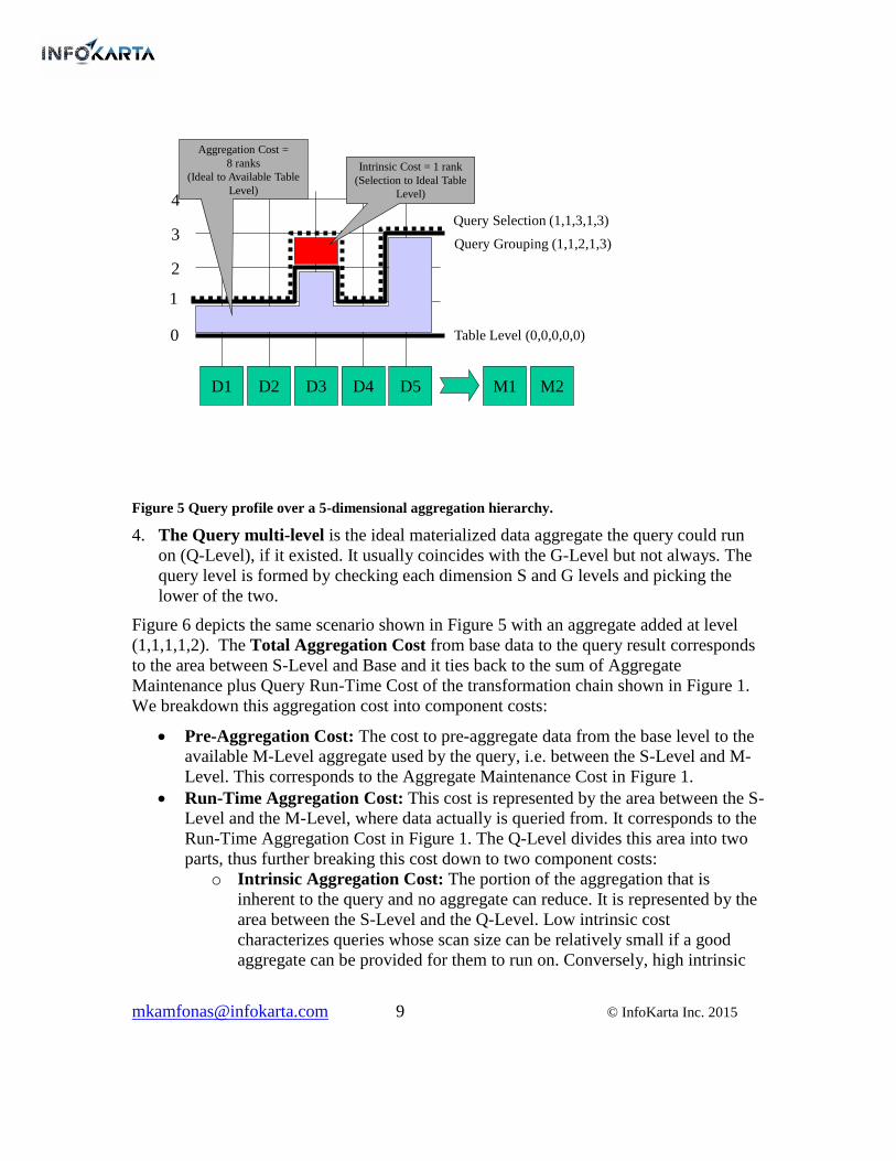
scan. Figure 5 shows our fact with five dimensions, the S-Level (dotted), G-Level

(solid) and the M-Level, in this case (0,0,0,0,0).



D1 D2 D3 D4 D5 M1 M2

Query Selection (1,1,3,1,3)

Query Grouping (1,1,2,1,3)

0

1

2

3

4

Table Level (0,0,0,0,0)

Intrinsic Cost = 1 rank

(Selection to Ideal Table

Level)

Aggregation Cost =

8 ranks

(Ideal to Available Table

Level)

Figure 5 Query profile over a 5-dimensional aggregation hierarchy.

4. The Query multi-level is the ideal materialized data aggregate the query could run

on (Q-Level), if it existed. It usually coincides with the G-Level but not always. The

query level is formed by checking each dimension S and G levels and picking the

lower of the two.

Figure 6 depicts the same scenario shown in Figure 5 with an aggregate added at level

(1,1,1,1,2). The Total Aggregation Cost from base data to the query result corresponds

to the area between S-Level and Base and it ties back to the sum of Aggregate

Maintenance plus Query Run-Time Cost of the transformation chain shown in Figure 1.

We breakdown this aggregation cost into component costs:

Pre-Aggregation Cost: The cost to pre-aggregate data from the base level to the

available M-Level aggregate used by the query, i.e. between the S-Level and M-

Level. This corresponds to the Aggregate Maintenance Cost in Figure 1.

Run-Time Aggregation Cost: This cost is represented by the area between the S-

Level and the M-Level, where data actually is queried from. It corresponds to the

Run-Time Aggregation Cost in Figure 1. The Q-Level divides this area into two

parts, thus further breaking this cost down to two component costs:

o Intrinsic Aggregation Cost: The portion of the aggregation that is

inherent to the query and no aggregate can reduce. It is represented by the

area between the S-Level and the Q-Level. Low intrinsic cost

characterizes queries whose scan size can be relatively small if a good

aggregate can be provided for them to run on. Conversely, high intrinsic



cost queries require large numbers of qualifying rows scanned per point

selected, even if the best possible aggregate existed for them to run on.

o Discretionary Aggregation Cost: This is the run-time cost incurred to

aggregate data from an available materialized aggregate up to the query

level, i.e. the area between the Q-Level and the M-Level. It is

discretionary since we chose to materialize at a lower level. Essentially,

introducing aggregates converts Discretionary to Pre-Aggregation cost.

D1 D2 D3 D4 D5 M1 M2

Query Selection (1,1,3,1,3)

Query Grouping (1,1,2,1,3)

0

1

2

3

4

Table Level (0,0,0,0,0)

Intrinsic Cost = 1 rank

(Selection to Ideal Table

Level)

Aggregate (1,1,1,1,2)

Aggregation Cost =

2 ranks

6 ranks of aggregation are

already in the aggregate

Figure 6 - Intrisic, discretionary aggregation and pre-aggregation cost separated

We can classify aggregation queries into distinct patterns based on the relative

positioning of these lines and their intrinsic cost. Figure 7 shows four such patterns:

1. Drill-Down Interactive Queries are typically initiated from a point the user selects and

requests a lower level drill down. The selected cells are at some “selection level” (S-

Level) and the drill-down level defines the “grouping level” requested (G-Level.) The

drill-down is typically the next level along one or two dimensions. In lattice terms,

the S and G levels are close to each other, maybe a couple of ranks apart, meaning

that only a few G-Level rows are required per S-Level selected. In other words, the

intrinsic cost is low and consequently sustaining interactive response times is feasible

as long as an aggregate exists “close enough” to any query level selected. The top left

diagram of the figure shows how from a selection level at (3,2,4,3,1) drilling down

along two dimensions delivers grouped data at (3,2,3,2,1). The red shaded area is

proportional to the intrinsic cost of the query.



Figure 7: Query patterns

2. Breakdown Reports are characterized by a relatively broad selection and relatively

low-level grouping of data e.g. select Product Categories X, Y and Z for last month

for this and last year, and return amounts and quantities sold by product class, by

store and day. Such a pattern is shown at the top-right diagram of Figure 7. These

queries have a high intrinsic cost because of the large distance between selection and

grouping levels. They can only be run on relatively low level detail and they require a

large number of rows. They are classified as “reports” since they can be rather

voluminous due to the level of detail they convey. This type of query may be used to

feed graphic visual components to plot highly detailed graphs, in those cases naming

their classification as “reports” may be too restrictive.

3. Mining and Hybrid Rollups are queries that select data along some or all dimensions

at levels lower that they group them. The lower diagrams of Figure 7 show such

query patterns mining low level data and rolling them up to cluster or classify them

along higher levels of the same dimensions. Select specific SKUs supplied by a list of

vendors last year and group them by class and district. This type of query needs to

mine data for specific products at the item level, and then roll-up counts and amounts

to higher levels of these taxonomies.

With this backdrop, let’s now look into how optimal levels are chosen and the details

behind their implementation.



Optimal Levels

Formality and General Practice

One school of thought is to “architect” aggregates during the data design process and

base them on application/reporting requirements that dictate what the hot spots are. This

inevitably results in hardwired aggregates, often modeled as prime structures and taking

life of their own, difficult to adjust and likely to leave large portions of the lattice

uncovered.

A different approach is to monitor the system workload and create aggregates when

needed in response to performance issues when they arise. This approach is adaptive and

responds to changing workloads, however it may lead to proliferation of costly high

proximity application-specific aggregates that are easy to add but hard to refactor. This in

turn is likely to interfere with their sustainability and evolution, leading to resource

saturation and premature need for capacity upgrades.

Analytic Approach

The approach we favor combines the “architected” with the “iterative” and it is based on

the following three premises:

Optimal aggregate selection is driven from the data itself; not directly dictated by

specific reporting requirements.

A rational framework for quantifying and analyzing performance is essential, and

optimization should take into account the total system, its workloads and service

levels.

Coupling of applications to aggregates must be avoided so that changes are

painless down the road.

We use two types of algorithms to determine optimal aggregates. One is a variation on

the technique proposed by Harinarayan, Rajaraman, and Ullman [1], which iteratively

seeks the “best next aggregate” that minimizes the sum of materialized rows scanned to

run the equivalent of “select *” at every vertex of the lattice. As higher level aggregates

get picked and their materialization factored into the model, this sum is reduced

progressively. The other is a VDM technique that sweeps the weighted loaded

aggregation lattice starting from the bottom, to select the closest node of “adequate

aggregation distance.” The algorithm iterates and as chosen aggregates are factored into

the model all vertices of the lattice end up “close enough” to some chosen aggregate thus

covering the whole lattice with heavier weighed nodes favoring hot spots.

The purpose of this paper, however, is less to explain algorithms, and rather to present

and rationalize the methodology, its premises and characteristics:

1. Optimal aggregations are best determined by the data topology and cardinalities

depicted in a properly weighed and loaded aggregation lattice. Requirements should



be used to construct, prune, load or weigh the lattice, but should not dictate aggregate

levels.

2. Maximize sharing. One common aggregate is better than two close ones over the

same fact supporting two different applications. There is one caveat to this, having to

do with autonomy and separation of concerns, and it is discussed separately in the

next section.

3. Odd but true: As a general rule the more effective the aggregates chosen to

materialize, the more expensive they will be to maintain. Chains of aggregates built

one on top of the other facilitate maintenance, but tend to leave large areas of the

lattice uncovered. Proper aggregate selection should provide complete coverage of

the lattice and address hot spots by weighing them accordingly.

4. Avoid trivial aggregations. Aggregating 100 billion rows into a 90 billion row

aggregate, at face value, makes a negligible improvement in performance and is not

worth the cost of its maintenance. Such close aggregates may only be justified if they

resolve other costly derivations, such as:

a. Pre-joining orders to Line items

b. Pivoting vertically organized health provider roles into flat easier queried

columns

c. Materializing derived columns that are used for filtering.

Such situations can often be addressed in the base model design, but by the time they

become an issue aggregates are the easier way to resolve them.

5. Avoid recastable aggregations if possible. If an as-is dimension participates in the

lattice, the lowest and highest levels are by definition non-recastable. Levels in

between may require restating historical aggregates if the hierarchy changes. Evaluate

the feasibility of pruning recastable multi-levels from the aggregation lattice.

Although good to avoid, recastable aggregates may be a necessary evil to achieve

desired service levels, and they should not be discarded a priori.

6. Follow the rule of proportionality: The magnitude of the work executed by the system

to ingest a data change and maintain all dependent structures must be proportional to

the magnitude of the change ingested. This is a generalization of the earlier point

about recasting. Examples where this rule may get violated are:

a. A change of one row of a dimension may impact millions of fact rows (as-is

recasting)

b. The use of MIN or MAX in an aggregate may cause history refresh if a row

that determined the minimum or maximum is removed

c. Data maintenance practices - Refreshing a dimension by replacing data as

opposed to merging changes will cause the whole dependent tower of

dependent JIs to be refreshed.

In most cases, proportionality violations can be fixed by tweaking scripts, adding an

index, running statistics, setting up proper constraints etc. It is important that these issues

get shaken out of the system before aggregates are considered. Aggregates should not be

used as a crutch or workaround to basic performance tuning.



Implementation Considerations

Aggregate Maintenance Automation – The Choices

There is no doubt that system-maintained data is the preferred method from the point of

view of data integrity and quality. From the perspective of performance, however, it can

be argued that user-maintenance methods can outperform automated methods in some

cases. For example, system maintenance that is row-at-a-time or constrained by

transaction boundaries leads to fragmentation, additional overhead and the possibility of

double updates where independent details fall under the same summary point. Deferred

system maintenance, if supported, can be an improvement. We encourage systematic

testing and relentless tuning and qualification of the available system-provided methods

before resorting to user-built solutions.

As a rule we discourage user-controlled solutions when system-controlled options are

available. There are cases, however, where materializing actual tables is appropriate. The

pros and cons vary by platform:

If an aggregate involves metrics that violate the proportionality principle, such as

MIN and MAX, it will not be incrementally maintained by the system, resorting

to full refresh.

o In DB2 a user maintained MQT is preferable because it can still be

recognized for optimization.

o In Teradata a user-maintained table may be a better choice with BI tools

providing query optimization through aggregate awareness features.

If a recastable (as-is) dimension is involved in an aggregation and we want to

avoid the unpredictability of real-time maintenance caused by dimension changes.

o DB2 deferred MQTs may provide adequate flexibility. User-maintained

MQTs may be a better and more predictable option. A VDM differential

recasting algorithm is provided.

o In Teradata deferred maintenance of JIs is not currently supported. If the

JI exposes unpredictability risk, a user-maintained aggregate table should

be considered, relying on BI tools for optimization.

The complexity of queries, after views are unraveled, may impact optimization

resulting in suboptimal plan selection, reduced estimation confidence or failure to

match JIs and MQTs. Low level facts can be materialized as independent tables

absorbing computation and join complexity. Simpler aggregates can then be built

on top.

Sharing, Autonomy and Separation of Concerns

Two data marts that share a sales fact should share its aggregates if both the conditions

below are met:

Similar non-conflicting dimensionality: If the same fact is used by two virtual

data marts, with the same or very close dimensionality, it is preferable to establish



one set of aggregates for both. If however the Product dimension requires “as-is”

semantics in one mart and “as-was” in the other, this makes the dimensions

conflicting. In this situation if recast-aggregates cannot be avoided they should be

separated.

Access views shall be aggregate agnostic: The ultimate objective behind this

requirement is decoupling applications from aggregates. If an aggregate is

removed or its level adjusted, applications may need to be tested but should not

have to be modified. Access layer views are treated as parts of the application.

Their change cascades to the applications that use them. Granted, building access

views over aggregate-definition views makes matching and redirection by the

optimizer safer. However this also exposes the user or application querying the

mart to be conscious of the aggregations. A better design is to establish access

views at the base level and capture all idiosyncrasies and computations there.

Such views are stable and can be used as the base for all aggregate definition

views at higher levels in the lattice. As long as they are straightforward

aggregations and all complexity and joins are captured into the base view, the

optimizer will detect the subsumption and redirect the queries.

To illustrate the point, Figure 8 shows a base fact with two dimensions combined

into a base view. The Base View is used in the two Application Access Views 3

and 4. There are also two system maintained aggregates with their respective view

definitions. Access Views 1 and 2 are specific to these aggregates. If applications

are exposed to them, then change of aggregate level will require the applications

to be changed as well. Decoupling the application entails reliance on access views

3 and 4 only. All queries will be directed to these views, and the optimizer shall

redirect to the aggregates whenever it recognizes that the query subsumes the

definition of these aggregates. In order to raise the likelihood that this will occur,

the base view must absorb all the complexity (filters, computations and joins) and

keep the Aggregate Views 1 and 2 as simple as possible. If access views are

aggregate agnostic, aggregate levels can be adjusted without requiring

applications to be modified, although as part of evaluating the change, their

queries must be benchmarked or tested.



Figure 8 – Application-Aggregate Coupling through aggregate-dependent views

Materialized aggregates are shared performance objects that belong with the

respective base data in the same spirit that indexes are. This idea, however, can

only be supported if we decouple applications from those performance enhancers,

as is the case with indexes. If we couple performance objects to access layer

views we delegate optimal aggregate selection to the application, and any change

to these aggregates challenges the “autonomy” of these applications. We

consequently propose that aggregate sharing is a virtue if and only if access views

and applications are aggregate agnostic.

Automation and Tools

Both during the construction of the lattice and the classification of queries, some level of

automation is desirable. Three specific use cases for such automation are:

Scan actual queries collected from monitoring the system and summarize statistics

of tables, views and columns involved.

Parsing queries to identify their multi-level. This allows us to monitor workloads

of queries and know their S-Level, G-Level, M-Level, Q-Level as well as the

discretionary and intrinsic cost and rank. This type of analysis is invaluable in

analyzing and quantifying performance impact when planning improvement

iterations and evaluating results after changes are made.

Constructing benchmarks from template patterns to evaluate coverage of the

lattice, performance improvements, check optimizer choices on use of aggregates

etc.

VDM includes customizable tools that can be adapted on a case by case basis. When

queries are generated from application tools such as MicroStrategy, the naming



conventions are consistent and simple scanners can achieve a reasonable level of success.

To the degree that this level of automation is feasible, and after a potentially tedious

initial setup, the repeatability of the process and the opportunity to systematically analyze

large samples of actually executed queries makes it worth the effort. Of course the ease of

such automation depends on access layer complexity and the consistency of naming

conventions

Conclusion

The VDM Aggregation Strategy provides a framework for identifying and refining

aggregates and the access layer. From prior applications in other industries, the

methodology may yield improvements as high as a level of magnitude. For existing

mature systems we typically set a modest target of 20% or 30% improvement of current

utilization for targeted periods and workloads. This translates into resource savings that

frees up capacity for additional work, and may elongate – or keep from shrinking –

capacity upgrade cycles

The process of implementing the VDM Aggregation Strategy is iterative, following these

rough steps:

1. Analyze query patterns, set targets and plan

2. Evaluate the access layer design for coupling with aggregates. Evaluate options

3. Create/Refine baseline model envelope; baseline benchmarks

4. Build, prune, load and weigh the aggregation lattice; map current aggregates

5. Analyze historical or projected workloads and generate benchmarks covering the

lattice to the extent possible – identify opportunities with existing JIs;

6. Determine optimal aggregates considering existing levels – propose changes and

additions

7. Benchmark and evaluate impact

8. Implement

9. Validate

Bibliography

[1] V. Harinarayan, A. Rajaraman, J. Ullman “Implementing Data Cubes Effectively”

ACM/SIGMOD June 1996, Montreal Canada p.205

[2] I. S. Mumick, D. Quass, B. S. Mumick “Maintenance of Data Cubes and Sumary

Tables in a Warehouse” ACM/SIGMOD 1997, AZ USA

[3] W. Lehner, R. Sidle, H. Pirahesh, R. Cochrane “Maintenance of Cube Automatic

Summary Tables” ACM/MOD Dallas, TX 2000.

[4] Yannis Kotidis, Nick Roussopoulos “DynaMat: A Dynamic View Management

System for Data Warehouses” ACM/SIGMOD 1999


vdm aggregation strategy - infokarta.com stragtegy - white paper...vdm aggregation strategy ......

Documents