veca - jan magnus · if a is an (m,n) matrix and aits jth column, then veca is the ran-column...
TRANSCRIPT
SIAM J. ALG. DISC. METH.Vol. i, No. 4, December 1980
(C) 1980 Society for Industrial and Applied Mathematics0196-5212/80/0104-0008, S01.00/0
THE ELIMINATION MATRIX: SOME LEMMAS ANDAPPLICATIONS*
JAN R. MAGNUS AND H. NEUDECKER*
Abstract. Two transformation matrices are introduced, L and D, which contain zero and unit elementsonly. If A is an arbitrary (n, n) matrix, L eliminates from vecA the supradiagonal elements of A, while Dperforms the inverse transformation for symmetric A. Many properties of L and D are derived, in particularin relation to Kronecker products. The usefulness of the two matrices is demonstrated in three areas ofmathematical statistics and matrix algebra: maximum likelihood estimation of the multivariate normaldistribution, the evaluation of Jacobians of transformations with symmetric or lower triangular matrixarguments, and the solution of matrix equations.
1. Introduction. If a matrix A has a known structure (symmetric, skew symmetric,diagonal, triangular), some elements of .4 are redundant in the sense that they can bededuced from this structure. Thus, if A is a symmetric or lower triangular matrix oforder n, its n(n-1) supradiagonal elements are redundant. If we eliminate theseelements from vecA (the column vector stacking the columns of A), this defines a newvector of order n(n+ 1) which we denote as v(A). The matrix which, for arbitrary A,transforms vecA into v(A) is the elimination matrix L, first mentioned by Tracy andSingh (1972) and later by Vetter (1975) and Balestra (1976).
Of equal interest is the inverse transformation from v(A) to vecA. For lowertriangular A, we shall see that L’v(A)fvecA. We further introduce the duplicationmatrix D such that, for symmetric A, Dv(A)=vecA. The matrix D (or a matrixcomparable to D) was previously defined by Tracy and Singh (1972), Browne (1974),Vetter (1975), Balestra (1976), and Nel (1978). D +, the MooreoPenrose inverse of D,possesses the property, used by Browne (1974) and Nel (1978), D +vecA v(A), forsymmetric A.
The purpose of this paper is to study the matrices L and D. Both matrices consistof zero and unit elements only. 2 gives the necessary definitions and basic tools. Thenext two sections contain the theoretical heart of the paper and establish a number ofresults on L and D. 5-7 are devoted to applications: maximum likelihood estima-tion of the multivariate normal distribution, the evaluation of Jacobians of transfor-mations with symmetric or lower triangular matrix arguments, and, finally, thesolution of matrix equations. An appendix presents the proofs of the lemmas in 4.
Not all results are new. Thus, Tracy and Singh (1972) established that ]L(A(R)A)D[= ]AI +1. They obtained two other determinants as well (their examples 5.3 and5.4), but these are both in error. Browne (1974) proved the important fact that(D’(A(R)A)D)- =D +(A-(R)A-)D +’ for nonsingular A, while Nel (1978) evaluatedthe determinant of D+(A(R)B)D, when ABffiBA, A and B symmetric. Concurrentlywith the present paper, Henderson and Searle (1979) wrote an article on the sametopic. Inevitably there is some overlap between the two papers.
2. Notation and preliminary results. All matrices are real; capital letters representmatrices; lowercase letters denote vectors or scalars. An (m, n) matrix is one having m
*Received by the editors September 26, 1978 and in final form February 7, 1980.tDepartment of Economics, University of British Columbia, 2075 Wesbrook Mall, Vancouver, Canada
V6T 1WS.*Institute of Actuarial Science and Econometrics, University of Amsterdam, 23 Jodenbreestraat, 1011
NH Amsterdam, Netherlands.
422
THE ELIMINATION MATRIX 423
rows and n columns; A’ denotes the__transpose of A, trA its trace, and [AI itsdeterminant. If A is a square matrix, A denotes the lower triangular matrix derivedfrom A by setting all supradiagonal elements in A equal to zero; dg(A) is the diagonalmatrix derived from A by setting all supra- and infradiagonal elements in A equal tozero. If x is an n-vector, and f(x)=(f(x).. "fm(X))’ a differentiable vector functionof x, then the matrix Of/Ox has order (n, m) with typical element (Of/Ox).
The unit vector ei, i= 1,..., n, is the ith column of the identity matrix I,, i.e., it isan n-vector with one in its th position and zeroes elsewhere. The (n, n) matrix Ej hasone in its 0"th position and zeroes elsewhere, i.e., Ej =eej. We partition the identity
n(n + 1) as follows"matrix of order
I(l/2)n(n+l)-’(ulIH21 UnlU22"’" Un2U33"’" Unn ).
n(n+ 1) with unity in its [(j-1)n+iFormally, u2 is a unit vector of order-- j(j- l)]-th position and zeroes elsewhere (1 <__j<__i<-n).If A is an (m, n) matrix and A its jth column, then vecA is the ran-column
vector
/t.
vecA
n(n + 1) vector that is obtained fromIf A is square of order n, v(A) denotes thevecA by eliminating all supradiagonal elements of A. For example, if n---3,
vecA (alia21a31a12a22a32a13a23a33and
v(A) (a,a2a3a22a32a33 )’.Finally, the Kronecker product of an (m, n) matrix A (aj) and an (s, t) matrix
B is the (ms, nt) matrix
A(R)B--(aijB ).This settles the notation. Let us now state some prelimina_ry results that will be
used throughout. If A--(aij) is an (n, n) matrix, then A, A, and dg(A) can beexpressed as
(2.1) A= E aijEij; Y= . ai2Eij; dg(A)= aiiEiiij ij i-----1
A standard result on vecs is
(2.2) vecABC-- (C’ (R)A )vecB,if the matrix product ABC exists. For vectors x and y of any order we then have
(2.3) x(R)y=vecyx’ and x(R)y’ =xy’ =y’(R)x.
The basic connection between the vec-function and the trace is
(2.4) (vecA)’vecB trA’B,
where A and B are (m, n) matrices. From (2.2) and (2.4) follows
(2.5) (vecA)’(B (R) C)vecD trA’CDB’,
if the expression on the right-hand side exists.
424 JAN R. MAGNUS AND H. NEUDECKER
We shall frequently use the commutation matrix K defined implicitly as"
DEHNTION 2.1a (implicit definition of K). The (n2, n2) commutation matrix Kperforms for every (n, n) matrix A the transformation KvecA =vecA’.
In fact, K is a special case of the (mn, mn) matrix Kmn which maps vecA intovecA’ for an arbitrary (m, n) matrix A. The matrix K, was introduced by Tracy andDwyer (1969). Many of its properties are derived in Magnus and Neudecker (1979),who also established the following explicit expression for K.
DEFINITION 2.1b (explicit definition of K).
i==lj-----1
Closely related to the commutation matrix is the matrix N.DEFINITION 2.2a (implicit definition of N). The (n2, n2) matrix N performs for
every (n, n) matrix A the transformation NvecA =vec1/2(A + A’).Its explicit expression is immediately derived.DEFICTION 2.2b (explicit definition of N).
N--1/2(I+K).Note that the implicit definitions of K and N are proper definitions in the sense
that they uniquely determine K and N. The following lemma gives some properties ofK and N.
LEt_A 2.1.(i) K--K’--K -"(ii) K(A (R) B) (B(R)A)K, for any (n, n) matrices A and B;(iii) N N’ N2;(iv) NK=N KN.
For any (n, n) matrix A we have(v) N(A (R)A)--- (A (R)A)N=N(A (R)A)N;(vi) N(I(R)A +A (R)I)=(I(R)A +A (R)I)N=N(I(R)A +A (R)I)N
2N(I(R)A )N-- 2N(A (R)I)N.Proof. The properties of K follow from Magnus and Neudecker (1979). The
properties of N follow from those of K since N
Let us now give four results on the unit vector u of order n(n + l) and the v(.)operator.
(2.6) , UijUj I(1/2>n(,+ 1)"i>=j
If A is an (n, n) matrix, then
(2.7) v(A)=v(Y)= aijuj and v(dg(A))=
(2.8) uij=v(Eij ) and aij=ujv(A ), i>__j;
(2.9) v(A) v(dg(A)), if A is upper triangular.
Finally, we make use of the following standard facts in matrix differentiation.For every matrix X and Y of appropriate orders,
(2.1O) d(XY) (dX) Y+X(dY),(2.11) dtrXr= tr(dX)Y+ trXdr.
THE ELIMINATION MATRIX 425
For every nonsingular X,
(2.12) dlog X trX ldX,
dX X l(dX )X 1.
3. Basic properties of L and D. Let us now introduce the elimination matrix L. Asin the previous section, where we defined K and N, the elimination matrix will bedefined implicitly and explicitly.
DEFINITION 3.1a (implicit definition of L). The (1/2 n(n+ 1), n2) elimination matrixL performs for every (n, n) matrix A the transformation LvecA---v(A).
L, thus defined, eliminates from vecA the supradiagonal elements of A. We shallshow that L is.uniquely determined by (3. a). Let A be an arbi.trary (n, n) matrix, andsuppose that L and L both transform vecA into v(A). Then (L-L)vecA =0 for everyA. Hence, L= L. We can derive an explicit expression for L as follows. Recall that ei,
i= 1.-- n, is the th unit vector of order n. Then, using (2.7), (2.4), and (2.3), we find
v(A ) i>jaijuij i>juij( e:Aej) E uijtr( eje;A )
Z uijtr(EiA) Z uij(vec Eij)’vecA Z(uij@ej(e;)vecA.ij ij i>j"
This leads to the following explicit definition.DEFINITION 3.1b (explicit definition of L).
L= E uij(vecEij)’= . (uij(R)e(R)e;).i>=j ij
An example, for n= 3, is
00
0 00
0
0 00 0
0 0 0 0
Most authors on (0,1) matrices are interested only in transformations withsymmetric matrices, and work with LN rather than L. See, e.g., Browne (1974) and Nel(1978). The justification for this lies in the following lemma.
LEMMA 3.1. For any (n, n) matrix A we have
(i) LNvecA - v(A +A’)
In particular, when A is symmetric,
(ii) LNvecA =v(A).
Proof. Immediate from the implicit definitions of N and L.
Thus, if A is symmetric, L and LN play the same role. In this paper we havechosen a more general approach, based on LvecA =v(A) for arbitrary A, largelybecause this allows us to study transformations with triangular matrices as well. Thefollowing lemma characterizes L as a (0, 1) matrix with i n(n + 1) l’s, one in each rowand not more than one in each column.

426 JAN R. MAGNUS AND H. NEUDECKER
LMMA 3.2.n(n+ 1)"(i) L has full row-rank
(ii) LL’ I/2)+ O;(iii) L + L’, where L+ is the Moore-Penrose generalized inverse of L.Proof. We shall show that LL’--I. The other two results then follow directly.
LL’= X (uijeje;) Z (U’hkekeh)= X (uijukejeke;eh)ij hk ij hk
ijj ](1/2)n(n+ 1), by (2.6).ij
Let us now determine three matrices that are useful for certain linear transfoations.LM 3.3. The matrices L’L, LKL’, and L’LKL’L are diagonala ideotent of
rank n(n+ 1), n, and n respectively. t A be an arbitra (n, n) trix. Then,
(i) L’LvecA vecA;(ii) L’L= (E@Eii);(iii) LKL’v(A) v(dg(A));
(iv) LKL’= iii;iffil
(v) L’LKL’LvecA vec(dg(A));
(vi) L’LKL’L (EiiEii ).il
Proof. By the explicit definition of L wc have
L’L= (ujejei) (Uhkee)= (ujuhkejeeie)ij hk ij hk
(ejeeie)= (EjjEii),ij ij
so that, using (2.2) and (2.1),
L’ w a (ij ij
vec ( eieAeje ) vec aijEijij ij
Further, for arbitra v(A),
aiiii iiiv(A),
by (i), the implicit definitions of K and L, (2.9), (2.7) and (2.8). is proves (i) and(iv). Silarly, for arbitra vecA,
L’LKL’LvecA L’v(dg(A )) vec(dg(A)) vec (auEu )
=vec (eieAeie)= vec(EiiAEii) ( EiiEii)vecA
by (iii), (i), (2.1) and (2.2). It is easy to see that the tee matrices are diagonal withonly zeroes and ones on the diagonal. Hence they are idempotent. era of each of

THE ELIMINATION MATRIX 427
n(n+ 1), n and nthe three matrices equals the number of ones on the diagonal, i.e.,respectively. [-]
Note that Lemma 3.3(i) implies that L’LvecA =vecA if and only if A is lowertriangular. The matrix LKL’, as shown in the previous lemma, is diagonal with n onesand n(n- 1) zeroes. Hence, I+ LKL’ is a nonsingular diagonal matrix with n times 2
L(I + K)L’and n(n- l) times on the diagonal. Because LNL’ =n(n 1) times1/2(LL’ + LKL’) 1/2(I+ LKL’), it is diagonal too with n times and
on the diagonal. The following properties of LNL’ are of interest.LEMMA 3.4. The matrix LNL’ is diagonal with determinant(i) LNL’I 2-(1/2)n(n-1).
Its inverse is
(ii) ( LNL’)- 2I- LKL’.Proof. Since LNL’ is a diagonal matrix, its determinant is the product of its
diagonal elements, i.e., ]LNL’ --2 -(l/2)n(n-D. Property (ii) is easily established usingLNL’ 1(1+ LKL’) and the idempotency of LKL’. [-]
As we have seen, L uniquely transforms vecA into v(A). The inverse transforma-tion generally does not exist. We can, however, easily transform v(A) into (the vecsof) a lower triangular matrix or a diagonal matrix, since
L’v(A)=vecA (Definition 3.1a and Lemma 3.3 (i)),and
L’LKL’v(A)=vecdg(A) (Definition 3.1a and Lemma 3.3(v)).Combining these two transformations one verifies that
( L’ + KL’- L’LKL’)v(A)=vec(Y+’-dg(A)).
We have thus found a matrix which transforms v(A) into (the vee of) a symmetricmatrix. Let us define this matrix implicitly.
n(n/ 1)) duplication matrixDEFINITION 3.2a (implicit definition of D). The (n2,D performs for every (n, n) matrix A the transformation Dv(A) vec(A +’ dg(A)).
It is easy to see that D is unique. Hence, D= L’+KL’-L’LKL’ =2NL’-L’LKL’.Note that in particular, if A is symmetric, DLvecA=Dv(A)=vecA. This is animportant property that we will frequently use. The converse is also true; i.e., any Asatisfying DLvecA vecA is symmetric.
LEMMA 3.5.(i) LD IOI2)n(n+ );(ii) OLN-- N;(iii) D-- 2NL’ L’LKL’ NL’(LNL’)- .Proof. Let A--A’; then LDv(A)=LvecA=v(A). Hence, LD--I, since the sym-
metry of A does not restrict v(A). Further, for arbitrary A,
DLNvecA=DLvec1/2(A +A’)--Dv(1/2(A +A’))---vec1/2(A +A’)--NvecA,which proves (ii). It also implies that DLNL’ =NL’, and because of the nonsingularityof LNL’, D NL’(LNL’)- . [-I
Note that DLN=N is a defining property of D. In fact, it is just a reformulationof Definition 3.2a. The matrix D can be explicitly expressed in terms of unit vectors of
428 JAN R. MAGNUS AND H. NEUDECKER
order i n(n + 1) and n, i.e., in terms of uij, ei, and ej. From the explicit definition of Kand L, and the expression for L’L (Lemma 3.3 (ii)), one verifies that
and
so that
Z,K--
LKL’L-- E Uu(vecEu)’,
D’ L+LK-LKL’L
E uij(vecEij)’+ E uij(vecEji)’- E Uu(vecEi,)’.ij ij
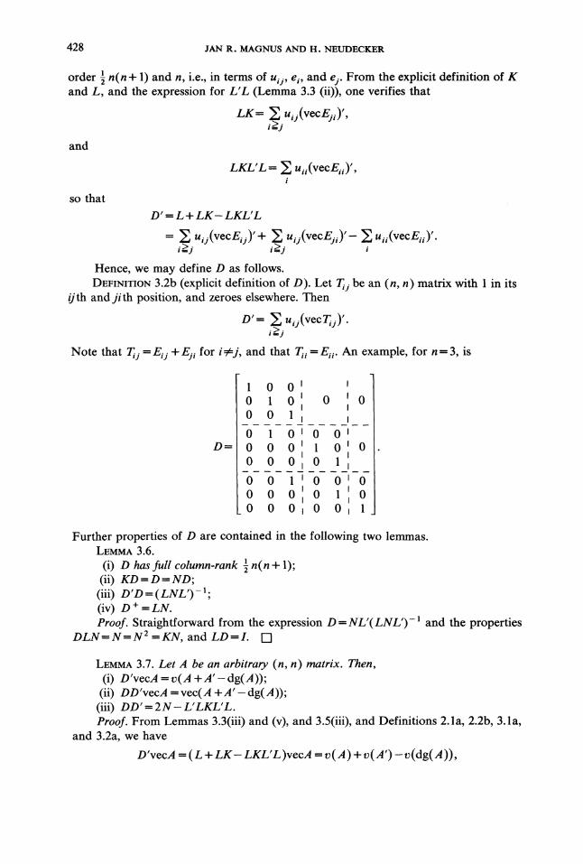
Hence, we may define D as follows.DFINITION 3.2b (explicit definition of D). Let T/j be an (n, n) matrix with in its
0"th and jith position, and zeroes elsewhere. Then
o’= ZNote that Tj Ej + Ej for i4:j, and that Tu Eu. An example, for n= 3, is
0 00 00 0
0 00 0 00 0 0
0 000 0
Further properties of D are contained in the following two lemmas.LEMtA 3.6.
(n+ 1);(i) D has full column-rank n(ii) KD D ND;(iii) D’O (LNL’)(iv) D + LN.Proof. Straightforward from the expression D=NL’(LNL’)- and the properties
DLN N N2 KN, and LD I.
LEMMA 3.7. Let A be an arbitrary (n, n) matrix. Then,(i) D’vecA =v(A +A’-dg(A));(ii) DD"vecA =vec(A +A’-dg(A));(iii) DD’ 2N- L’LKL’L.Proof. From Lemmas 3.3(iii) and (v), and 3.5(iii), and Definitions 2.1a, 2.2b, 3.1a,
and 3.2a, we have
D’vecA (L +LK-LKL’L)vecA v(A) + v(A’) v(dg(A)),
THE ELIMINATION MATRIX 429
and
DD’vecA =Dv(A +A’-dg(A))=vec(A +A’- dg(A))(I+K)vecA L’LKL’LvecA (2N- L’LKL’L)vecA,
for an arbitrary (n, n) matrix A. Hence, DD’ =2N-L’LKL’L.
The matrices L and D, like the commutation matrix K, are useful in matrixdifferentiation. From Definition 2.1a, it follows that vecX/vecX’=K where X is an(n, n) matrix. The corresponding results for L and D are contained in the followinglemma.
LEMMA 3.8. Let X be an ( n, n) matrix. Then[ L, for lower triangular X;
(i) vecX/v(X)= D’, for symmetric X;(ii) Ov(X)/OvecX L’.Proof. Immediate from the relations vecX= L’v(X) (lower triangular X), vecX=
Dv(X) (symmetric X), and v(X)=LvecX. [-]
Comment. More general results are easily obtained from Lemma 3.8, using thechain rule. In particular, let Y=F(x) be an (n, n) matrix whose elements aredifferentiable functions of a vector x. Then
( Ov(Y)/Ox)L if Y is lower triangular for all x;(i) vecY/19x
()v(r)/Ox)D’ if Y is symmetric for all x;(ii) Ov(Y)/Ox--(OvecY/Ox)L’ for all Y.
4. Applications to Kronecker products. From 2 we know that the commutationmatrix K possesses two major properties: a transformation property, KvecA =vecA’(its definition), and a Kronecker property, K(A (R)B)K=B(R)A. The elimination matrixL and the duplication matrix D have likewise been defined by their transformationproperties, viz. LvecA=v(A) and, for symmetric A, Dv(A)=vecA. Let us nowinvestigate their Kronecker properties. The applications in 5-7 are based almostentirely on the lemmas in the present section. Proofs are postponed to the Appendix.
We shall first show that, if A and B have a certain structure (diagonal, triangular),Kronecker forms of the type L(A (R)B)L’ and L(A (R)B)D often possess the samestructure.
LEMM 4.1. Let A and M be diagonal n-matrices with diagonal elements i and #g( 1... n). Letfurther P and Q be lower triangular n-matrices with diagonal elements Piiand qii, i= 1... n. Then,
(i) L(A(R)M)L’ =L(A(R)M)D is diagonal with elements tikj(i__.J") and determi-nant IIitii-i+ 1.
(ii) L(P(R) Q)L’ is lower triangular with diagonal elements qgiPjj(i >-) and determi-n--i+l.nant IIiqiiPii
(iii) L(P(R)Q)D is lower triangular and L(P’(R)Q’)D is upper triangular. Bothmatrices have diagonal elements qiipjj(i>=j") and determinant _i _n-i+
HiqiiPiiNext we establish some properties of L(P’(R) Q)L’, with lower triangular P and Q.
Notice that (i) is the Kronecker counterpart of the property L’LvecP--vecP for lowertriangular P.
LEMM 4.2. For lower triangular n-matrices P (Pij) and Q= (qij),(i) L’L(P’(R)Q)L’=(P’(R)Q)L’;

430 JAN R. MAGNUS AND H. NEUDECKER
(ii)1,2,- ,
[L(p,(R))L,I,L[(p,),(R)Q,IL, s ,-2,- 1, ifP -1 and Q-1 exist,
s--g, if lower triangular pl/2 and Ol/ exist;
(iii) L(P’(R)Q)L’=D’(P’(R)Q)L’ has eigenvalues qiiPjj (i>=J) and determinant_i _n--i+
i1iiPiiIn Lemma 4.1 we have proved that, for lower triangular P and Q, the matrices
L(P(R)Q)L’, L(P(R)Q)D, L(P’(R)Q’)L’, and L(P’(R)Q’)D are triangular as well, withdiagonal elements qiiP22, i>=J Although the matrices L(P’(R)Q)L’, L(P(R)Q’)L’, andL(P(R)Q’)D are not triangular, they also possess eigenvalues q,P22, i>=J; see Lemma4.2. The matrix L(P’(R)Q)D is more complicated and seems not to have such niceproperties. In particular, its eigenvalues are in general different from q,P22, i>-
The results of Lemmas 4.1 and 4.2 enable us to find the following determinantswhich are of importance in the evaluation of Jacobians of transformations with lowertriangular matrix arguments (see 6).
LEMMA 4.3. For lower triangular n-matrices P, Q, R, and S with diagonal elementsp,, q,, r,, and sii, i= 1.-. n, we have
(i) IL(PQ’(R)R’S)L’ -’IXi(riisii)i(Piiqii)n-i+ 1;(ii) [L(P’(R)Q+ R’(R)S)L’I-IIi> j(qiiPjj +siiGj);(iii) IL(P(R)Q’R)DI-- IIi(-qiirii) tlii(iv) IL(PQ’(R)R’)DI ---IIiriii(Piiqii)n-i+ 1.
If P, Q, R, S are nonsingular,(v) [L(PQ’(R)R’S)L’]-=L(Q’-(R)S-)L’L(P-(R)R’-)L’.
Finally,H
(vi) IL [(P’)n-h(R)Ph-]L’IfHnIPIH-IIi>jlXi2 H=2,3,---,h=l
where(pi , -e 7)
IJ’ij (Pii --Pjj)ifpii 51=PJJ’
H-InPii ifPii-’Pjj.A variety of corollaries flow from Lemma 4.3 by putting one or more of the
LEMMA 4.4. For any (n, n) matrix A,(i) DL(A (R)A)D--’(A (R)A)D;
(ii) [L(AA)D]" =L(AS(R)AS)D, ifA exists,
ifA1/2 exists;
matrices P, Q, R, and S equal to I. Also, the four matrices L(PQ’(R)Q’P)L’,L(PQ’(R)P’Q)L’, L(PQ(R)Q’P)D, and L(PQ’(R)P’Q’)D have the same determinant,namely el/ Ol/.
In Lemmas 4.1-4.3 we have studied triangular matrices only. The crucialproperties for lower triangular matrices are L’LvecP=vecP and its Kronecker coun-terpart L’L(P’(R)Q)L’--(P’(R)Q)L’, which enable us to discover further properties ofthe important matrix L(P’(R)Q)L’. Let us now turn away from triangular matrices.An equally important property is DLvecA =vecA for symmetric A. Its Kroneckercounterpart is DL(A (R)A)D=(A (R)A)D for arbitrary A, as we shall see shortly, and itenables us to study the matrix L(A (R)A)D.
THE ELIMINATION MATRIX 431
(iii) The eigenvalues of L(A(R)A)D are XiXj, i>-, when A has eigenvaluesXi(i=l...n);
(iv) Iz(a(R)a)Ol--Ial"+;(v)
IfA is nonsingular,(vi) [D’(A (R)A)D] LN(A-@A- )NL’.
IfAB BA, and A and B have eigenvalues h and lzi, i-- 1... n,(vii) [D’(A (R)B)D[-- IA[ IBIIIi>j(AiIj -I-ji).Note that in (vii) we do not require A and B to be symmetric, in contrast to Nel
(1978). In applying (vii) one must be careful to note that knowledge of h and/1 is notsufficient in order to compute IIi>j(,dj +hjlxi). In general, it is necessary to carryout the simultaneous reduction of A and B to diagonal form, because the ordering ofthe eigenvalues is important. A case that can be solved without this reduction is
ID’(A’(R)Aq)DI=IAI "+"q (Xf-q +x-q),i>j
where p and q are integers (positive, negative or zero).Similar results hold for the Kronecker sum I(R)A +A (R)1:LEMMA 4.5. For any (n, n) matrix A with eigenvalues h ( 1... n),(i) DL(I(R)A +A(R)I)D=(I(R)A +A(R)I)D--2N(I(R)A)D--2N(A(R)I)D;(ii) the eigenvalues of L(I(R)A +A (R)I)D are h +Xj, i>-_j’;(iii) IL(I(R)A +A(R)I)DI--2"IAIII,>j(A, +hi);(iv) [L(I(R)A +A(R)I)D] - =L(I(R)A +A(R)I)-D;
for nonsingular I(R)A +A (R)I. The results (i) and (iii) can be generalized toH H
(v) DL (A-n(R)Aa-)D (A-n(R)Aa-)D, H--2,3,...,hffil h--l
andH
(vi) IL (An-n(R)Ah-1)Dl=H’lAl"-’IIi>jlxij,h--1
where
H=2,3,-..,
ftij (i--kj)if ’i
H--IHX if k
The next lemma concerns the detenant of the sum or the difference of thematrices L(A@A)D and L(BB)D.
LEM 4.6. Let A and B be (n, n) mtrices. Then the detemint
IL(A@AXB@B)DIequals
(i) A + i](1 AiAj), ifA is nonsingular and hi, 1... n, are the eigenvaluesof BA -"
(ii) ij(auajj biibjj), if Af(aij) and Bf(bij) are lower trianlar;(iii) Hij(PiPj Oi’), ifABfBA, where Pi and #i (iffi 1... n) denote the eigenvaV
ues of A and B.Again, owledge of p and is, in general, not sufficient to compute (iii). See
the remarks under Lena 4.4(vi).A final lemma will prove useful in 5 and 6.
432 JAN R. MAGNUS AND H. NEUDECKER
LEMMA 4.7. Let P be a lower triangular and nonsingular (n, n) matrix, and a ascalar. Let
(i) IL[e’(R)e+avecP(vece’)’]L’l=( +an)lel"+;(ii) L[ P’ (R) e + avece(vecP’)’]L’)- L[P’- 1(R) e flvecP l(vecP’- I)’]L’,
where a/(1 + an). Let further A be a symmetric and nonsingular (n, n) matrix. Then,(iii) L[A (R)A + avecA(vecA)’]D ( + an)l A["+ 1;(iv) [L[A (R)A + avecA(vecA)’]D -1 L[A l(R)A -1 _/3vecA -l(vecA-I)’]D.This ends the theoretical part of this paper.
5. Maximum likelihood estimation of the multivariate normal distribution. Weshall now show the usefulness of L and D in a number of applications. Consider asample of size m from the n-dimensional normal distribution of y with mean/t andpositive definite ovariance matrix O. The maximum likelihood (ML) estimators of/tand are well known, but the derivation of these estimators is often incorrect. Theproblem is to take properly into account the symmetry conditions on O, as hasrecently been stressed by Richard (1975) and Balestra (1976). More precisely, weshould not differentiate the likelihood function with respect to veer, but with respectto v(O). First we derive the ML estimators of /t and (Lemma 5.1), then theinformation matrix and asymptotic covariance matrix (Lemma 5.2), and finally weinvestigate properties of the random vector v(F), an unbiased estimator of v(O).
LEMMA 5.1. Consider a sample of size m from the n-dimensional normal distribution
of y with mean /t and positive definite coariance matrix 0. The maximum fikelihoodestimators of/t and are
(it= - . y,=-Y;
),.
Proof. The loglikelihood function for the sample is
mlogAm(y;/t, v(O}) " nmlog2r- - trO IZ,
where m
Z---- E (Yi--/t)(Yi--/t)’"i---1
Using well-known properties of matrix differentials (see (2.10)-(2.13)) and traces(2.4)-(2.5), the first differential of A can be written as
mdlogl OdA - - tr(d - )Z- i tr dZ
mtrtI) ldtI) + IZ- trO l(dO)O
+ "trO- (Yi-/t)(d/t)’ + (d/t) E (Yi
ltr(ddp)O-l(Z-mO)0-1 + (d/t)’O-I (Yi --/t)2
!(vecdO)’(o-lo-1)vec(Z-mO)+(d/t)’O-I E (Yi2
-(dv(O))’D’(O-lo-l)vec(Z-m*)+(d/t)’O-l E (Yi
THE ELIMINATION MATRIX 433
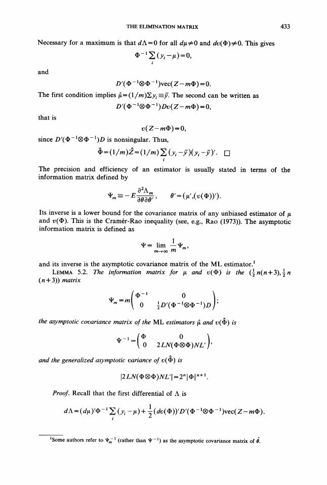
Necessary for a maximum is that dA=0 for all d/v0 and dv()vO. This gives-1Z (yi --/) =0
and
D’( -1@ -1)vec(Z_me) =0.
The first condition implies f=(1/m)Y,y -----. The second can be written as
D’( -’(R) 1)Dv(Z-me) 0,
that is
v(Z-mt) O,
since D’(-(R) )D is nonsingular. Thus,
=(1/m)=(1/m) (Yi --)(Yi--)" 1-]
The precision and efficiency of an estimator is usually stated in terms of theinformation matrix defined by
02Am O’xI E)0)0’
Its inverse is a lower bound for the covariance matrix of any unbiased estimator ofand v(). This is the Cram6r-Rao inequality (see, e.g., Rao (1973)). The asymptoticinformation matrix is defined as
xI,= lim xI,,,,,m-- oo m
and its inverse is the asymptotic covariance matrix of the ML estimator.LEMMA 5.2. The information matrix for t and v() is the (-2 n(n+3), in1
(n + 3)) matrix
-1 o ).--1( --1-1D’( )D
the asymptotic covariance matrix of the ML estimators f and v() is
0 2LN((R))NL’
and the generalized asymptotic variance of v() is
I2LN( (R)dp)NL, 2,,11.+ 1o
Proof. Recall that the first differential of A is
--1 --1dA=(d)’-l (Yi --P’)+ (dv())’D’( )vec(Z-m
1Some authors refer to XIml (rather than xI,-1) as the asymptotic covariance matrix of d.

434 JAN R. MAGNUS AND H. NEUDECKER
The second differential is therefore
d2A=(d)’(de-l) E (Y,-)-m(d)’*-’(d)
’D’( -1))vec(Z+ -(dv(dp)) d(dp-’(R)dp --map)- -1, )v c(aZ-maO).
Taking expectations, and observing that Ey =, EZ=m, and EdZ=O, we find
( m )(dv()),D,(-l 1)vecdEaA=m(att)’ ’( at, ) + -[m ,(=m(d)’-(dt)+l,T1(dv(,))’D - (R)- )Ddv(O).
The information matrix then follows. From Lemma 4.4 we know that
and
Hence,
and
D’(*- l)(I)-1)DI 2(l/2)n(n- 1)11-("+ 1).
o )2LN(r(R)O)NL’
12LN(p(R)dp)NL’ 2(’/2),,("+ l) D’(O -1() (I) --’)DI -’
=2(1/2)n(n+l)2-(1/2)n(n-1)ld#l"+l=2nldPl"+l. i--]
The ML estimator v()) is not an unbiased estimator of v(). Let us therefore define
Fm
y" (Yi--Y)(Yi __y)t_. mo"m--1
The following properties of v(F) can then be established.
LEMMA 5.3. The random vector v(F) is an unbiased estimator of v(dp),(i) Ev(F) v().
Its covariance matrix is
(ii) cov(v(F))=2(LN(dp(R)dp)NL’)/(m- 1),and v(F) is therefore a consistent estimator of v(dp). In particular,
(iii) var(fy)=(qi +qiiqyj)/(m- 1), i>__j"= 1... n.Finally, the efficiency of v(F) is
(iv) eff(t(F))’--[(m- 1)/m](1/2)n(n+ l).Proof. We know that
mS= X (yi-Y)(yi-Y)’= Xyiy;-myg’
is centrally Wishart distributed W(m-1, ), see Rao (1973, p. 537). Therefore, asderived in Magnus and Neudecker (1979, Corollary 4.2),
me,=(m- )O,

THE ELIMINATION MATRIX 435
and
cov(mvec) (m 1)( I+K)(@).Thus, v(F)--(m/(m-1))v()is an unbiased estimator of v() and its covariancematrix is
cov(v(F)) 1cov(mv()) 1cov( Lvecm)(m-l))- (m-l)
(m- 1)2.(m--1)L(I+K)(dp(R)d)L’
2 2.LN((R))L’= .LN((R))NL’.
(m-l) (m--l)We see that cov(v(F))0 as mo. This shows that v(F) is a consistent estimator ofv(), given (i). The diagonal elements of LN(tb(R))NL’ can be derived as follows.Let i>_; then, by (2.8), Lemma 3.3 (i), and (2.5),
u;jLN(dp@d# )NL’uij ( v( Eij ))’LN(d@d# )NL’v( Eij)
(vec( Eij + Eji ))t(f(f)vec( Eij +Eft)
Thus,
2
var(f/j)(m- 1) qij + qiiqjj).
Finally, the efficiency of v(F) is [see Anderson (1958, p. 57)]
-EO2A-1
Ov(O)0v(O)’eef(v(F))=
Icov(v(F))l
2)NL’(m 1)
-I
-D’(dp dp )D
----I (m--l)-1
Lemmas 5.1 and 5.2 can be straightforwardly generalized by allowing the Yi tohave different expectations/i. Clearly, it is not possible to estimate all/ (i= 1.-- m)
In(n+ 1) parameters, from nm observations. If, however, weand v(), i.e., nm+ -assume that the/ depend upon a fixed number of parameters (01- 0r)=0’, and/ isthe ML estimator of 0, then the ML estimator of is
(1)= Y. (Y,-li())(Yi-ti())"and the asymptotic covariance matrix of v() is again
as.cov(v()) 2LN(dp(R)O)NL’.

436 JAN] R. MAGNUS AND H. NEUDECKER
6. Jacobians. Let the matrix Y be a one-to-one function of a matrix X. Thematrix J J(Y, X) (vecY/0 vecX)’ is called the Jacobian matrix and its determi-nant the Jacobian of the transformation of X to Y.
Because the ordering of the variables is arbitrary, the value of the Jacobian canvary in sign, but since only the absolute value matters, this should not worry us. Notethat our. definition of a Jacobian differs from some textbooks’, where J(Y, X) isdefined as I vecY/vecX 1.
Consider for example the linear transformation
Y=AX,where X and Y are (m, n) matrices, and A is a nonsingular (m, m) matrix. Takingdifferentials and vecs we have
dY=AdX,and
so that
dvecY=(I(R)A)dvecX,
IJ(Y,X)I=)vecY
OvecX =II(R)AI--IAI"
The evaluation of Jacobians of transformations involving symmetric or lowertriangular matrix arguments is not straightforward, since in this case X contains onlyn(n + 1) "essential" variables. To account for this, a variety of methods have been
used, notably differential techniques (Deemer and Olkin (1951) and Olkin (1953)),induction (Jack (1966)), and functional equations induced on the relevant spaces(Olkin and Sampson (1972)). Our approach finds its root in Tracy and Singh (1972)who used modified matrix differentiation results to obtain Jacobians in a simplefashion.
n(n + 1) variables Yij and the i n(n + 1)Consider the relation between the ivariables xij given by
Y=AXA’,where X (and hence Y) is symmetric. Taking differentials and vecs, we have
dvecY=(A(R)A)dvecX,and, using the definitions of L and D,
dv(Y) L(A (R)A )Ddv(X),so that by Lemma 4.4 (iv)
IJ(Y,X)I=Ov(X)
--IL(A(R)A)DI--IAI "+’.
See also Deemer and Olkin (1951), Anderson (1958, pp. 156 and 162), Jack (1968),Tracy and Singh (1972), and Olkin and Sampson (1972). Anderson unnecessarilyassumes that X has a Wishart distribution or that A is triangular. A more generaltransformation is
Y=AXA’ +_. BXB’,where X again is symmetric. This yields
dv(Y)=L(A<A +_.BB)Ddv(X),and the Jacobian matrix is
J( Y, X)=L(A &A ++_ B(R)B)D,

THE ELIMINATION MATRIX 437
of which we know the determinant from Lemma 4.6. See Tracy and Singh (1972) foran earlier (wrong) solution in the case AB--BA.
We now turn to nonlinear transformations involving symmetric matrix arguments.Consider
Y=XAX,where A and X are symmetric. Differentiating,
dr= (dX) X+X(dX)so that
and
dvecY= (XA (R)I+ I(R)XA)dvecX,
dr(Y) L(XA (R)I+ I(R)XA)Ddv(X).Thus, from Lemma 4.5 (iii), the Jacobian is
IJ(Y, X)I=[L(XA(R)I+I(R)XA)DI=2"]AI]X ]-[ (h +hj),i>j
where hi, i= 1..-n, are the eigenvalues of XA. This problem has been studied byTracy and Singh (1972), but not solved satisfactorily. See also Olkin and Sampson(1972).
The inverse transformation
y=x -,for symmetric X gives
av( r) L(X ’(R)X ’)Dav(X)Disregarding the minus sign, the Jacobian is (Lemma 4.4 (iv))
IJ(Y, X)l-- lt(x-l(R)x-1)Ol--lXl --(n+l).
See Jack (1968), Zellner (1971, pp. 226 and 395), and Olkin and Sampson (1972).Zellner assumes (unnecessarily) that X is positive definite.
More interesting is the transformation, again for X--X’,
y--ISiS -l.Totally differentiating yields
dV--(dlXl)X -I +lgldX -I
---IX I(trX -dX)X -ISiS -(dX)X -’,so that
and
dvecY= IX I[ (vecX ’)(vecX 1)’dvecX- (X -l(R)x 1)dvecX]-IXl[ X-Ix-I-(vecX-1)(vecX-1)’]dvecX,
dv( Y) -[XIL[ x l(R)x -’ (vecX )(vecX ) ] Dd)(X).The Jaeobian is
Jar(y, X)l--IX <l/)"<"+ ’)ILl X -l(x -1 (vecX l)(vlcX -l)t] D--Ixl(l/)"("+’)(1-n)lXl-<"+’) (by Lemma 4.7 (iii))
--(n-- 1)lxl ’/-"+’"-=>.
438 JAN R. MAGNUS AND H. NEUDECKER
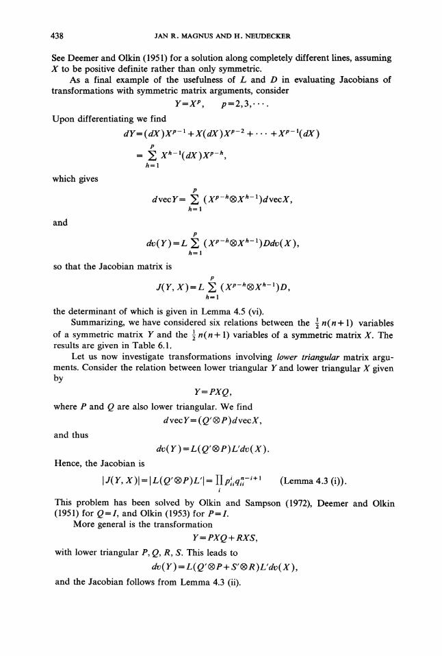
See Deemer and Olkin (1951) for a solution along completely different lines, assumingX to be positive definite rather than only symmetric.
As a final example of the usefulness of L and D in evaluating Jacobians oftransformations with symmetric matrix arguments, consider
Y=X’, p=2,3,’".
Upon differentiating we find
ar=(ax)x -’ +x(ax)x +...P
E x -’(dX)Xh.
which givesP
dvecY= ] (X’-h(R)Xh-)dvecX,h---I
andP
dv(Y)=L , (X’-h(R)Xh-’)Ddv(X),h--I
so that the Jacobian matrix isP
J(Y, X)=L E (X’-n@Xn-I)o,h--1
the determinant of which is given in Lemma 4.5 (vi).n(n+ 1) variablesSummarizing, we have considered six relations between the i
of a symmetric matrix Y and the i n(n + 1) variables of a symmetric matrix X. Theresults are given in Table 6.1.
Let us now investigate transformations involving lower triangular matrix argu-ments. Consider the relation between lower triangular Y and lower triangular X givenby
Y= PXQ,where P and Q are also lower triangular. We find
dvecY=(Q’(R)P)dvecX,and thus
dv(Y ) L(Q’ (R)P)L’dv(X ).Hence, the Jacobian is
IJ(Y, X)I=IL(Q’(R)P)L’I= ]-IPiiqii -i+l (Lemma 4.3 (i)).
This problem has been solved by Olkin and Sampson (1972), Deemer and Olkin(1951) for Q=I, and Olkin (1953) for P=I.
More general is the transformation
Y=PXQ+RXS,with lower triangular P, Q, R, S. This leads to
dv(Y)=L(Q’(R)P+ S’(R)R)L’dv(X),and the Jacobian follows from Lemma 4.3 (ii).

THE ELIMINATION MATRIX 439
TAnLE 6.1Jacobians of transformations with symmetric matrix arguments
Transformation Jacobian J(Y, X)l Conditions, particularities
(i)
(ti)
(iii)
(iv)
(v)
(vi)
Y=AXA’
Y AXA’ +BXB’
Y=XAX
YffiX’ (pffi2,3,...)
IAln+ lij.(l +-hihy)
(aiiajj +-biibjj)i>_j
(, +_ooj)*
i>j
Ixl--(n+ 1)
(n- 1)lxl0/2"+ .-2)
plXl- II
*See the remarks under Lemmas 4.4 (vi) and 4.6 (iii).
IAI=0Ihl=/=O, hi (iffi l. n)
eigenvalues of BA
A =(aij and B,f(bij
lower triangular
ABffiBA, Ii and 0 (iffi 1... n)
eigenvalues of A and B
AffiA’,Ai(i=l...n
eigenvalues of XA
Ixl*0Ixl0
(xf-x;)/(x,-xs), ifij
p)k-1 if )k
where A (i 1..- n) areeigenvalues of X
Next, we consider the relation between symmetric Y and lower triangular X givenby
Y= B’XA +A’X’B.Using the same technique, we have
dvecY= (A’ (R)B’)dvecX+ ( B’ (R)A’)dvecX’A’ (R)B’ + (B’ (R)A’)K] dvecX (Definition 2.1a),
and
dv(Y)=L[ A’(R)B’ +(B’(R)A’)K]L’dv(X).The Jacobian is
by the definition of N and Lemmas 2.1 (ii), 3.5 (ii), and 3.4 (i). The determinant[L(A (R)B)D] can of course be evaluated for each specific A and B. In particular, ifA P and B Q’R, or A PQ’ and B R’, where P, Q, and R are lower triangular, wecan express this determinant in terms of the diagonal elements of P, Q, and R, byLemma 4.3 (iii)-(iv). Special cases have been solved by Deemer and Olkin (1951)(A =P’ and B=I) and by Olkin (1953) (A---1 and B=P).
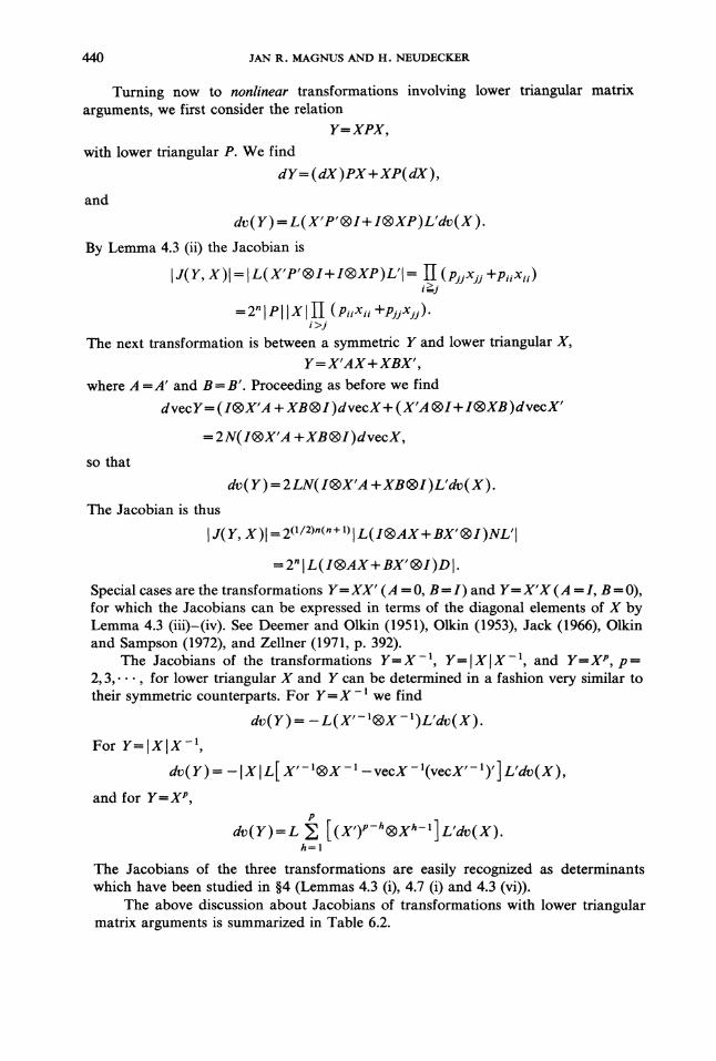
440 JAN R. MAGNUS AND H. NEUDECKER
Turning now to nonlinear transformations involving lower triangular matrixarguments, we first consider the relation
Y XPX,with lower triangular P. We find
at= (ax )ex+xe(ax)and
dv( r) L(X’P’ (R)I+ I(R)XP)L’dv(X ).By Lemma 4.3 (ii) the Jacobian is
IJ(Y, X)I=IL(X’P’(R)I+I(R)XP)L’I I (px +PiiXii)
--=lel IXl II (PiiXii-["pjjxjj).>j
The next transformation is between a symmetric Y and lower triangular X,Y=X’AX+XBX’,
where A---A’ and B---B’. Proceeding as before we find
dvecY=(I(R)X’A +.XB(R)I)dvecX+ (X’A (R)I+ I(R)XB)dvecX’
=2N(I(R)X’A +XB(R)I)dvecX,so that
dv( Y) 2LN(I(R)X’A +XBI)L’dv(X).The Jacobian is thus
[J(Y, X)] 2(1/2).(.+ 1) IL(I(R)AX+ BX’(R)I)NL’[
2"IL ( I(R)AX+ BX’ (R)I)D[.Special cases are the transformations Y=XX’ (A =0, B=I) and Y=X’X (A =I, B=0),for which the Jacobians can be expressed in terms of the diagonal elements of X byLemma 4.3 (iii)-(iv). See Deemer and Olkin (1951), Olkin (1953), Jack (1966), Olkinand Sampson (1972), and Zellner (1971, p. 392).
The Jacobians of the transformations Y=X 1, y= [X[X 1, and Y--X’, p2, 3,.-., for lower triangular X and Y can be determined in a fashion very similar totheir symmetric counterparts. For Y=X- we find
dv(Y ) I( x’ l(R)x 1)’dv(X).For Y--Ixl x-,
dv(Y) -ISlt[ X’- (R)X vecX (vecX’- )’ Z’dv(S ),and for Y X’,
P
av(r)= X [(X’)-hx-l]Z:av(X).h-’-I
The Jacobians of the three transformations are easily recognized as determinantswhich have been studied in 4 (Lemmas 4.3 (i), 4.7 (i) and 4.3 (vi)).
The above discussion about Jacobians of transformations with lower triangularmatrix arguments is summarized in Table 6.2.
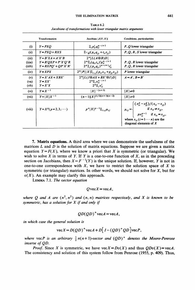
THE ELIMINATION MATRIX 441
TABLE 6.2Jacobians of transformations with lower triangular matrix arguments
Transformation Jacobian J(Y, X)l Conditions, particularities
(i)
(ii)
(iii)(iiia)(iiib)
Y--PXQ
(v)(va)(vb)
Y-- PXQ+RXS
Y-- B’XA +A’X’BY-- R’QXP+ P’X’Q’RY=RXPQ’ + QP’X’R’
II 9i _n-i+ir ii ttii
II (p.qjj +r.sn)2"IL(A@B)DI
2 n--i+IIi( qiirii) Pii2nIIi(Piiqii)n-i+ lr/i
P, Q lower triangular
P, Q, R, $ lower triangular
P, Q, R lower triangularP, Q, R lower triangular
(iv) YfXPX 2"IPI IxlII,>tp,,x,, +pjjxn) P lower tdangular
A--A’,B--B’2"IL(I(R)AX+ BX’ (R)I)DI2nIIix.-i+l
2 IIixii
Y=X’AX+XBX’Y=XX’Y--X’X
(vi) Y--X-’ Ixl-(n-t-l) IXlO(vii) Y--IXIX -1 (n- 1)lxl <’/zx"+ l"--) IXlO
p" Xlp- II i>flxiy(viii) YfXP(p---2,3, I.tij if Xii =i/=Xjj
pxfi-- if Xtiwhere xii (iffi 1-’- n) are thediagonal elements of X
7. Matrix equations. A third area where we can demonstrate the usefulness of thematrices L and D is the solution of matrix equations. Suppose we are given a matrixequation Y= F(X), where we know a priori that X is symmetric (or triangular). Wewish to solve X in terms of Y. If Y is a one-to-one function of X, as in the precedingsection on Jacobians, then X--F-I(Y) is the unique solution. If, however, Y is not inone-to-one correspondence with X, we have to restrict the solution space of X tosymmetric (or triangular) matrices. In other words, we should not solve for X, but forv(X). An example may clarify this approach.
LEMMA 7.1. The vector equation
QvecX-vecA,
where Q and A are (n2, n2) and (n, n) matrices respectively, and X is known to besymmetric, has a solution for X if and only if
QD(QD)+vecA vecA,
in which case the general solution is
vecX= D(QD)+vecA + D[ I- (QD) +QD ]vecP,where vecP is an arbitrary n(n+ 1)-vector and (QD) + denotes the Moore-Penroseinverse of QD.
Proof. Since X is symmetric, we have vecX---Dv(X) and thus QDv(X)=vecA.The consistency and solution of this system follow from Penrose (1955, p. 409). Thus,
442 JAN R. MAGNUS AND H. NEUDECKER
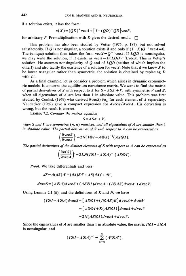
if a solution exists, it has the form
v(X ) (QD) +vecA + I- (QD) + QD vece,for arbitrary P. Premultiplication with D gives the desired result. [5]
This problem has also been studied by Vetter (1975, p. 187), but not solvedsatisfactorily. If Q is nonsingular, a solution exists if and only if (I-K)Q-lvecA =0.The (unique) solution then takes the form vecX=Q-lvecA. If LQD is nonsingular,we may write the solution, if it exists, as vecX=D(LQD)-LvecA. This is Vetter’ssolution. He assumes nonsingularity of Q and of LQD (neither of which implies theother!) and also tacitly the existence of a solution for vecX. Note that if we know X tobe lower triangular rather than symmetric, the solution is obtained by replacing Dwith L’.
As a final example, let us consider a problem which arises in dynamic economet-ric models. It concerns the equilibrium covariance matrix. We want to find the matrixof partial derivatives of S with respect to A for S =ASA’ + V, with symmetric V and S,when all eigenvalues of A are less than in absolute value. This problem was firststudied by Conlisk (1969) who derived OvecS/aij for each element of A separately.Neudecker (1969) gave a compact expression for OvecS/OvecA. His derivation iswrong, but the result is correct.
LEMMA 7.2. Consider the matrix equation
S=ASA’ + V,when S and V are symmetric (n, n) matrices, and all eigenvalues ofA are smaller thanin absolute value. The partial derivatives of S with respect to A can be expressed as
( )vecS ),3 vecA 2N( I(R)I-A (R)A )-1(AS(R) I).
The partial derivatives of the distinct elements of S with respect to A can be expressed as
)vecA 2LN(I(R)I-A @A)-I(AS@I).
Proof. We take differentials and vecs"
dS=A(dS)A’ +(dA)SA’ +AS(dA)’ +dV,
dvecS=(A (R)A)dvecS+(AS(R)I)dvecA +(I(R)AS)dvecA’ +dvecV.
Using Lemma 2.1 (ii), and the definitions of K and N, we have
( (R)I-A (R)A)dvecS= [ AS(R)+ ( I(R)AS)K] dvecA + dvecV
AS(R)I+K(AS(R)I)]dvecA + dvecV
2N(AS(R)l)dvecA + dvecV.
Since the eigenvalues of A are smaller than 1 in absolute value, the matrix I(R)I-A (R)Ais nonsingular, and
(I(R)I-A@A)-’= " (AhAh).h,=O
THE ELIMINATION MATRIX 443
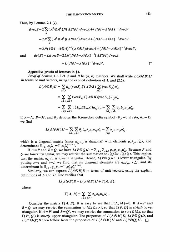
Thus, by Lemma 2.1 (v),
dvecS-- 2 (An(R)Ah )N( aS(R)I)dvecA + ( I(R)I-A (R)A)- ldvech
=2N", (Ah(R)Ah)(AS(R)I)dvecA +(I(R)I-A(R)A)-ldvecVh
--2N(I(R)I-A(R)A)-I(AS(R)I)dvecA +(I@I-A@A)-ldvecV,and dv(S)=LdvecS=2LN(I(R)I-A(R)A)-l(AS(R)I)dvecA
+ L(I(R)I-A (R)A)- ldvecV.
Appendix: proofs of lemmas in 4.Proof of Lemma 4.1. Let A and B be (n, n) matrices. We shall write L(A (R)B)L’
in terms of unit vectors, using the explicit definition of L and (2.5).
i>=j s
Y E (vecEij)’(A(B)(vecEst)uiju’s,i>--__js>t
X tF(EjinEsta’)uijust-- Z ajtbisuijusti>=j s>-_
If A A, B M, and ij denotes the Kronecker delta symbol (8i =0 if :/:j, 8u 1),we find
L(A(M)gt= i>:j s> jtisXjl’LiUijU;t Z XjLiUijUj’----t i>----j
which is a diagonal matrix (since UijUj is diagonal) with elements Li)kj, i>=j", anddeterminant IIi>_ fiziX IIi]Liik-i+ 1.
If A =P and B=Q, we have L(P(R)Q)L’ =Yi>j s>=t Pjtqisuijust. Because P andQ are lower triangular, we may restrict the summation to i>=j >-t, i>=s>=t. This impliesthat the matrix uiju’t is lower triangular. Hence, L(P(R)Q)L’ is lower triangular. Byputting s=i and t=j, we find that its diagonal elements are qiiPjj, i>-, and itsdeterminant is IIi>_j qiiPjj II _i _n-i+
iqiil)ii
Similarly, we can express L(A (R)B)D in terms of unit vectors, using the explicitdefinitions of L and D. One verifies that
(A (R))D (A(R))’ + r(A, ),where
I’(A, B) E E ajsbituiju’s,.i>--_j s>t
Consider the matrix F(A, B). It is easy to see that F(A, M)=0. If A=P andB Q, we may restrict the summation to >___d" >s > t, so that F(P, Q) is strictly lowertriangular. If A P’ and B Q’, we may restrict the summation to s > t >-i >=j’, so thatF(P’, Q’) is strictly upper triangular. The properties of L(A(R)M)D, L(P(R)Q)D, andL(P’(R)Q’)D then follow from the properties of L(A(R)M)L’ and L(P(R)Q)L’. W]
444 JAN R. MAGNUS AND H. NEUDECKER
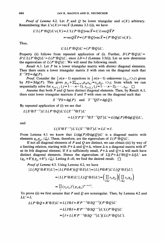
Proof of Lemma 4.2. Let P and Q be lower triangular and v(X) arbitrary.Remembering that L’v(X)--vecX (Lemma 3.3 (i)), we have
Thus,
L’L(P’ (R) Q )L’v(X) L’L( P’ (R) Q)vecX L’LvecQXP
vecQXP= ( P’(R) Q)vecX ( P’ (R)Q )L’v(X ).
L’L(P’(R)Q)L’=(P’(R)Q)L’.Property (ii) follows from repeated application of (i). Further, D’(P’(R)Q)L’=D’L’L(P’(R)Q)L’ =L(P’(R)Q)L’, since LD---I (Lemma 3.5(i)). Let us now determinethe eigenvalues of L(P’(R)Q)L’. We will need the following result.
Result A.1. Let P be a lower triangular matrix with distinct diagonal elements.Then there exists a lower triangular matrix S with ones on the diagonal such thats-eS=dg(e).
In(n--1) equations in n(n-1) unknowns (sij, i>j) givenProof. Consider the iby PS=Sdg(P). This gives Pij+,ih_j+lPihShj=Sijpjj, i>j, from which we cansequentially solve for sj+ 1, (J= 1..- n- 1), s+2, (j= 1.-- n-2),-.-, sn. I-’1
Assume that both P and Q have distinct diagonal elements. Then, by Result A.1,there exist lower triangular matrices S and T with ones on the diagonal such that
S PS dg(P) and T QT=dg(Q).
By repeated application of (i) we see that
L(S’@ T-’)L’L( P’(R)Q)L’L(S’- ’(R)T)L’L( S’P’S’-1(R) T -IQT)L’=L(dg(P) (R)dg(Q))L’,
and
L(S’(R)T-’)L’L(S’-’(R)T)L’=LL’=I.From Lemma 4.1 we know that L(dg(P)(R)dg(Q))L’ is a diagonal matrix withelements q,pj, i>=j". These, therefore, are the eigenvalues of L(P’(R)Q)L’.
If not all diagonal elements of P and Q are distinct, we can obtain (iii) by way ofa limiting relation, starting with P+ A and Q+ A, where A is a diagonal matrix with 8has its h th diagonal element. If is sufficiently small, P+ A and Q+ A will each havedistinct diagonal elements. Hence the eigenvalues of L[(P+A)’(R)(Q+A)]L’ are(q, +Si)(p +), i>_. Letting 6---0, we find the desired result. I"]
Proof of Lemma 4.3. Using Lemma 4.2, we have
L(eo’ (R)R’S)L’I L( P(R)R’)(Q’ (R)S)L’I L( P(R)R’)L’L(Q’(R)S)L’I
1[ siiqjj-IL(P’(R)R)L’IIL(Q’(R)S)L’I=(i>.jriiPjJ)(i>j
)H (riisii)i(Piiqii)n-i+ l.
To prove (ii) we first assume that P and Q are nonsingular. Then, by Lemma 4.2 andLL I,
L(P’(R) + R’(R)S)L’=L(I(R)I+ R’P’-’(R)SQ-’)(P’(R)Q)L’
=L(1(R)1+ R’P’-’(R)SQ-’)L’L( P’(R)Q)L’(1+ L( R’P’-’(R)SQ -’)L’)( L(P’ (R)Q )L’).
THE ELIMINATION MATRIX 445
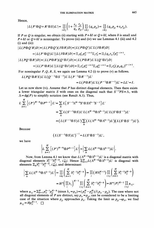
Hence,
iIj ( Sii J ) ijIL(P’(R)Q+R’(R)S)L’I-- -t’-- (qiiPjj)--’-- H (qiiPjj -’Siij)"qii Pjj ij
If P or Q is singular, we obtain (ii) starting with P+1 or Q+I, where is small andP+ 8I or Q+1 is nonsingular. To prove (iii) and (iv) we use Lemmas 4.1 (iii) and 4.2(i) and (iii)"L(P(R)Q’R)DI= L(P(R)Q’)(I(R)R)D I-- L(P(R)Q’)L’L(I(R)R)DI
_i _n--i+=IL(P’(R)Q)L’IIL(I@R)DI=HiqiiIii Hirii=Hi(qiirii)Pi-’+1
L( PQ’ (R)R’)DI= [L( P(R)R’)( Q’ (R)I )D I= L( P(R)R’)L’L(Q’@I)Dn--i+ i+1 n--i+l--IL(P’(R)R)L’IIL(Q (l)Dl--IIiriiPii lIIiqi- --IIirii(Piiqii)
For nonsingular P, Q, R, S, we again use Lemma 4.2 (i) to prove (v) as follows.
L( PQ’ (R)R’S)L’L( Q’- l(s -1)L’L(P -’(R)R’-
L(P(R)R’)L’L(P -’(R)R’-’)L’-- LL’-- I.
Let us now show (vi). Assume that P has distinct diagonal elements. Then there existsa lower triangular matrix S with ones on the diagonal such that S-IpS=A, withA dg(P) to simplify notation (see Result A. 1). Thus,
L [(P’)H-h(ph-1]L’-- EL[St-IAH-hs’SAh-Is-I]Lh--1 h
Because
we have
L(S’-I@S)L’L(A-h@Ah-’)L’L(S’@S-’)Lh
=(L(S’-’@S)L’) Z (L(AH-h@An-I)L’)(L(S’@S-’)L’)h
( L(S’-l(S)L’) -1= L( S’(S -I)L’,
L E [(P’)H-h@ph-1] L’hl
E L(AH-h(Ah-1)L’h
Now, from Lemma 4.1 we know that L(AH-h(Ah-1)L is a diagonal matrix withdiagonal elements xh/--lhjH--h, t’>’--__,/. Hence Y.ff.. IL(An-h@Ah-)L is diagonal withelements v xh- IxH-h i’, and deternant
L(g-h@h-l)L’ 2 .-lxj-h (-1) N -lxjh i4" hffil hffil
Hwhere ftij -X= lphii ,_n-hpjj (since k --Pii)-.(piHi --pjj )/(Pii--Pjj)" The case where notall diagonal elements of P are distinct, say p, =pjj, can be considered to be a limitingcase of the situation where pjj approaches Pii. Taking the limit as Pjj--Pii, we findIij HPiHi -1 [-]

446 JAN R. MAGNUS AND H. NEUDECKER
Proof of Lemma 4.4. Using the properties DLN=N, D=ND, and (A(R)A)N=N(A(R)A)--see Lemmas 3.5 (ii), 3.6 (ii), and 2.1 (v)--we have
DL(A (R)A)D DL(A @A)ND DLN(A@A)D N(A@A)D=(A(R)A)ND=(A(R)A)D.
This proves (i). By repeated application of (i) we find (ii). To prove (iii) we note thatn(n- 1)L(A(R)A)D and DL(A(R)A) have the same set of eigenvalues apart from i
zeroes which belong to the latter matrix. Let A have eigenvalues h and eigenvectorsxi; then
DL(A (R)A)(x(R)xj + x.i(R)xi)= DL(Axi(R)Axj +Axj(R)Ax)=XiXDL(x,(R)xj + xj(R)xi)-- X,XjDLvec(xjx=X,:vec(x:x +xxj) (by the implicit definition of D)
=XX(x(R)x + x(R)x).Hence, DL(A(R)A) has eigenvalues XX:, i>__j", plus g n(n-1) zeroes, and L(A(R)A)Dhas eigenvalues X),:, i>-_j". Its determinant is
L (A @A )D i>.j x ’j I[)k]+lIAIn+l’iLet us now prove (v) and (vi). Since D--NL’(LNL’) -1 (Lemma 3.5 (iii)), and
again using Lemmas 3.6 (ii) and 2.1 (v), we can write
D’(A A)D=(LNL’)-ILN(A (R)A)D=(LNL’)-IL( (R)A)D.The properties of D’(A (R)A)D thus follow from the properties of LNL’ (Lemma 3.4)and L(A (R)A)D (this lemma).
To prove (vii) we first assume that A has distinct eigenvalues. In that case thereexists a matrix T such that T- 1AT= A, where A is a diagonal matrix containing theeigenvalues of A. From AB=BA we have TAT- 1B--BTAT-, or AM--MA, whereM-- T- IBT. Since all X’s are distinct by assumption, M is diagonal. Hence it containsthe eigenvalues of B. We may then write
D’(A (R)B)D D’(rat 1() rMr -1)D D’( r(R) r)(h(R)M)(r -1) T -I)D
D’(T(T)L’D’(AIM)DE(T -11T -I)D,by (i). Hence, using (iv), the explicit definition of N, and Lemmas 3.5 (iii), 2.1 (ii), 3.4(i), and 3.6 (ii),
D’(aB)DI= D’(h(R)M)DI=I(LNL’)-ILN(h(R)M)DI
1L(I+K)(A(R)M)D[---ILNL’I -115--ILNL’I- 12-(1/2)n(n+ l) lg(AIM)D "t- L(M(A
=2-"IL(A(R)M+M(R)A)D I.
From Lemma 4.1 we know that L(A(R)M)D and L(M(R)A)D are diagonal matriceswith elements/zij and i/zj, i_._j’. The determinant of their sum is

THE ELIMINATION MATRIX 447
and thus
D’(A (R)B)DI=2 l-[ (t,X.i +kilJ,j)=2-nH (2Xil3,i) 1-[ (I,l,ikji>--_j i>j
=IAIIBI II (tLi)kj’t’)kitgj)i>j
If A has multiple eigenvalues, say i =j, we consider this as a limiting case ofthe situation where ,j approaches ,i- Taking the limit as Xj--->Xi the result follows. I--!
Proof of Lemma 4.5. From Lemma 2.1 (vi) and the properties ND---D andDLN= N, follows (i). The proof of (ii) is similar to that of Lemma 4.4 (iii). Property(iii) follows from (ii). Property (iv) follows from (i) since LD=I. We find (v) byrepeated application of DL(I(R)A+A(R)I)D=(I(R)A+A(R)I)D, and Lemma 4.4 (i).Let us prove (vi). We proceed as in the proof of Lemma 4.3 (vi). If A has distincteigenvalues (or if A =A’), there exists a nonsingular matrix S such that S-AS=A,where A is a diagonal matrix containing the eigenvalues of A. Thus,
H
L E (An-h(R)Ah-’)D=L., (SAn-hS-’(R)SAh-’S-’)Dh=l h
=L(S(R)S) _, (An-h(R)Ah-’)(S-’(R)S-’)Dh
=L(S(R)S)DL., (AH-h(R)Ah-’)DL(S-’(R)S-’)D,h
by Lemmas 4.4 (i) and 4.5 (v). Since L(S-(R)S-)D=(L(S(R)S)D) -, and usingLemma.4.4 (ii), we have
H
Lh,=l =ILE (AH-h(R)Ah-’)D
h
Lemma 4.1 tells us that L(AH-hAh-1)D is a diagonal matrix with elementskhi 1)tH h >-. Hence,.j
L (AH-h@Ah-1)D iI>J H-h H-1
hl hl
with
E -*=h--1 (X --Xj)
If A has multiple eigenvalues, i--kj say, we again consider this as a limiting case ofthe situation where , approaches ,i. Taking the limit as Aj--->)i we find #j =HX,n.-1.
Proof of Lemma 4.6. We shall only consider the determinant of the sum ofL(A (R)A)D and L(B(R)B)D. The determinant of their difference is proved in the sameway. By Lemma 4.4 (i),
L(A@A +B@B)D=(I+L(BA-I@BA-1)D)L(A@A)D.If BA- has eigenvalues ,, i= 1... n, L(BA-(R)BA-)D has eigenvalues XiXj, i>_,
448 JAN R. MAGNUS AND H. NEUDECKER
by Lemma 4.4 (iii), so that, using Lemma 4.4 (iv),
IL(A(R)A +n(R)n)Ol---- (1 +kikj)lhl "+1.
To prove (ii) we first assume that A is nonsingular. Then,
IL(A(R)A +BB)DI=IAI+1 + (a,ayj +b,byy),>j" a,aj
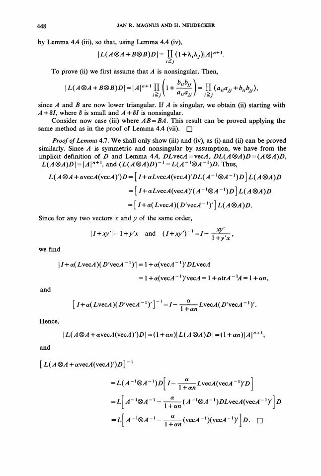
since A and B are now lower triangular. If A is singular, we obtain (ii) starting withA + 8I, where d is small and A +I is nonsingular.
Consider now case (iii) where AB=BA. This result can be proved applying thesame method as in the proof of Lemma 4.4 (vii).
Proof of Lemma 4.7. We shall only show (iii) and (iv), as (i) and (ii) can be provedsimilarly. Since A is symmetric and nonsingular by assumption, we have from theimplicit definition of D and Lemma 4.4, DLvecA=vecA, DL(A(R)A)D=(A(R)A)D,IL(A(R)A)DI--IAI "+l, and (L(A(A)D) -l --L(A-I@A-)D. Thus,
L(A (R)A + avecA(vecA)’)D I+ aLvecA(vecA)’nL(A -l(A -l)n L(A (R)A)D
I+ aLvecA(vecA)’(A-’(A-’)D] L(A (R)A)D
[ I+ a( LvecA)( D’vecA ’)’] L(A (R)A)D.
Since for any two vectors x and y of the same order,
[I+xy’l= +y’x and (I+xy’)-l=I+y’x
we find
I1+ a(LvecA)( D’vecA 1)’ + a(vecA )’DLvecA
+a(vecA- )’vecA + atrA-IA + an,
and
I+ a( LvecA)(D’vecA )’] -’ I-+an LvecA(D’vecA )’.
Hence,
[L(A@A +avecA(vecA)’)Dl=(1 +an)IL(A(R)A)DI=(1 + an)lAI "+1,
and
L(A (R)A +avecA(vecA)’)D] -a=L(A-(R)A-1)D I-+an
LvecA(vecA )’D
=L[A_(R)A_ a
+an (A (R)A )DLvecA(vecA -)’] D=L[A_I(R)A_ a
+an (vecA )(vecA 1),] D.
THE ELIMINATION MATRIX 449
REFERENCES
[1] T. W. ANDERSON, An Introduction to Multivariate Statistical Analysis, Wiley, New York, 1958.[2] P. BALESTRA, La drivation matricielle, Collection de I’IME, no. 12, Sirey, Paris, 1976.[3] M. BROWNE, Generalized least squares estimation in the analysis of covariance structures, South African
Statist. J., 8 (1974), pp. 1-24.[4] J. CONLISK, The equilibrium covariance matrix of dynamic econometric models, J. Amer. Statist. Assoc.,
64 (1969), pp. 277-279.[5] W. L. DEEMER AND I. OLKIN, The Jacobians of certain matrix transformations useful in multivariate
analysis, Biometrika, 38 (1951), pp. 345-367.[6] H. V. HENDERSON AND S. R. SEARLE, Vec al vech operators for matrices, with some uses in Jacobians
and multivariate statistics, Canad. J. Statist., 7 (1979) pp. 65-81.[7] H. JACK, Jacobians of transformations involving orthogonal matrices, Proc. Roy. Soc. Edinburgh Sect. A,
67 (1966), pp. 81-103.[8] J. R. MAGNUS AND H. NEUDECKER, The commutation matrix: some properties and applications, Ann.
Statist., 7 (1979), pp. 381-394.[9] D. G. NEL, On the symmetric multivariate normal distribution and the asymptotic expansion of a Wishart
matrix, South African Statist. J., 12 (1978), pp. 145-159.[10] H. NEtrDECKER, Some theorems on matrix differentiation with special reference to Kronecker matrix
products, J. Amer. Statist. Assoc., 64 (1969), pp. 953-963.[11] I. OLION, Note on ’The Jacobians of certain matrix transformations useful in multivariate analysis’,
Biometrika, 40 (1953), pp. 43-46.[12] I. OLrdN AND A. R. SAMPSON, Jacobians of matrix transformations and induced functional equations,
Linear Algebra and Appl., 5 (1972), pp. 257-276.[13] R. PENROSE, A generalized inverse for matrices, Proc. Cambridge Philos. Soc., 51 (1955), pp. 406-413.[14] C. R. RAo, Linear Statistical Inference and its Applications, 2nd ed., John Wiley, New York, 1973.[15] J. F. PdCHARD, A note on the information matrix of the multivariate normal distribution, J. Econometrics,
3 (1975), pp. 57-60.[16] D. S. TRACY AND P. S. DWYER, Multivariate maxima and minima with matrix derivatives, J. Amer.
Statist. Assoc., 64 (1969), pp. 1576-1594.[17] D. S. TRACY AND R. P. SINGH, Some modifications of matrix differentiation for evaluating Jacobians of
symmetric matrix transformations, Symmetric Functions in Statistics, D. S. Tracy, ed., University ofWindsor, Windsor, Ontario, 1972.
[18] W. J. VETTER, Vector structures and solutions of linear matrix equations, Linear Algebra and Appl., 10(1975), pp. 181-188.
[19] A. ZELLNER, An Introduction to Bayesian Inference in Econometrics, John Wiley, New York, 1971.