Vector Calculus

Vector Fields

ReadingTrim 14.1−→ Vector Fields

Assignmentweb page−→ assignment #9

Chapter 14 will examine a vector field.

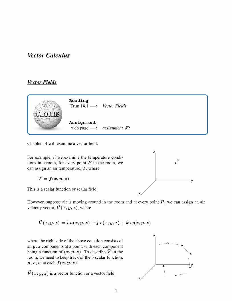
For example, if we examine the temperature condi-tions in a room, for every point P in the room, wecan assign an air temperature, T , where

T = f(x, y, z)

This is a scalar function or scalar field.x

y

z

P

However, suppose air is moving around in the room and at every point P , we can assign an airvelocity vector, ~V (x, y, z), where

~V (x, y, z) = i u(x, y, z) + j v(x, y, z) + k w(x, y, z)

where the right side of the above equation consists ofx, y, z components at a point, with each componentbeing a function of (x, y, z). To describe ~V in theroom, we need to keep track of the 3 scalar function,u, v, w at each f(x, y, z).

~V (x, y, z) is a vector function or a vector field.x

y

z

1

Gradient, Divergence and Curl Operations

The basic operator is the del operator given as

2D

∇ = i∂

∂x+ j

∂

∂y

3D

∇ = i∂

∂x+ j

∂

∂y+ k

∂

∂z

The del operator operates on a scalar function, such as T = f(x, y, z) or on a vector function,such as ~F = iP + jQ+ kR (force) or ~V = iu+ jv + kw (velocity).

We will examine three operations is more detail

1. gradient:∇ operating on a scalar function

Examples include the temperature in a 2D plate, T = f(x, y)

∇T = i∂f

∂x+ j

∂f

∂y

or for a 3D volume, such as a room

∇T = i∂f

∂x+ j

∂f

∂y+ k

∂f

∂z

The physical meaning was given in Chapter 13. ∇T is a vector perpendicular to the Tcontours that points “uphill” on the contour plot or level surface plot.

2. divergence:∇ dotted with a vector function→ ∇ · ~VWe can define the velocity in a 3D room as

~V (x, y, z) = iu(x, y, z) + jv(x, y, z) + ku(x, y, z)

DIVERGENCE of ~V = div ~V = ∇ · ~V

∇ · ~V =

(i∂

∂x+ j

∂

∂y+ k

∂

∂z

)·(iu+ jv + kw

)=∂u

∂x+∂v

∂y+∂w

∂z

The DIVERGENCE of a vector is a scalar.

2

3. curl: the vector product of the del operator and a vector,∇× ~V , produces a vector

curl of ~V = curl ~V = ∇× ~V

∇× ~V =

(i∂

∂x+ j

∂

∂y+ k

∂

∂z

)×(iu+ jv + kw

)

≡

∣∣∣∣∣∣∣∣∣i j k∂

∂x

∂

∂y

∂

∂zu v w

∣∣∣∣∣∣∣∣∣

= i

∂w∂y − ∂v

∂z︸ ︷︷ ︸V1

+ j

∂u∂z − ∂w

∂x︸ ︷︷ ︸V2

+ k

∂v∂x − ∂u

∂y︸ ︷︷ ︸V3

= i V1 + j V2 + k V3

The 3D case gives

curl ~V = i

∂w∂y − ∂v

∂z︸ ︷︷ ︸V1

+ j

∂u∂z − ∂w

∂x︸ ︷︷ ︸V2

+ k

∂v∂x − ∂u

∂y︸ ︷︷ ︸V3

The 2D case gives

curl ~V = k

(∂v

∂x−∂u

∂y

)

4. Laplacian: (∇ · ∇) operation.

A primary example of the Laplacian operator is in determining the conduction of heat in asolid. Given a 3D temperature field T (x, y, z), the Laplacian is

∂2T

∂x2+∂2T

∂y2+∂2T

∂x2= 0

3

2D example

Consider a 2D heat flow field, ~q(x, y).

Look at a small differential element, ∆x∆y. In steady state, heat flows in is equivalent toheat flow out. Therefore

∇ · ~q = 0 (1)

But ~q is related to temperature by Fourier’s law

~q = −k∇T (2)

Combining (1) and (2)

∇ · (−k∇T ) = 0→ ∇2T = 0

This is Laplace’s equation in 2D, which gives the steady state temperature field.

Example 4.1

Show for the 3D case f(x, y, z) that curl grad f = 0

∇f = i∂f

∂x+ j

∂f

∂y+ k

∂f

∂z

holds for any function f(x, y, z), for instance

f(x, y, z) = x2 + y2 + y sinx+ z2

4

Conservative Force Fields and the curl grad f = 0 identity

Suppose we have a conservative field ~F (x, y, z). We know ~F is irrotational, i.e.

∇× ~F = 0 (1)

(zero work in a closed path in the field)

But the identity says

∇× (∇φ) = 0 (2)

always holds when φ(x, y, z) is a scalar function.

Comparing (1) and (2)→ for a Conservative Force Field, we can always find a scalar functionφ(x, y, z) such that

~F = ∇φ

where φ is called the scalar potential function.

Sometimes, for convenience, we introduce a negative sign

~F = −∇u

The following statements are equivalent

~F is a conservative ⇐⇒ net work when a particle moves throughforce field ~F around a closed path in space is zero

⇐⇒ ∇× ~F = 0 irrotational

⇐⇒ a scalar function φ(x, y, z) can be found such that~F = ∇φ or a function u(x, y, z) can be foundsuch that ~F = −∇u

5

Line Integrals of Scalar Functions

ReadingTrim 14.2−→ Line Integrals

Assignmentweb page−→ assignment #10

One place that line integrals often come up is in the computation of averages of a function.

2D Case

x

2

2

f

L

f =1

L

∫ Lx=0

f(x)dx

3D Case

The temperature in a room is given by T =f(x, y, z). A curve C in the room is givenby x(t), y(t) and z(t). If we measure tem-perature along curve C, what is the averagetemperature T ?

T =1

L

value of f along C︷ ︸︸ ︷∫Cf(x, y, z)

arc length of C︷︸︸︷dS︸ ︷︷ ︸

line integral along C

L

x

y

z

t=0(S=0)

(S=L)t=

Calculation of the line integral along C

∫ αt=0

f [x(t), y(t), z(t)]︸ ︷︷ ︸f values along C

√√√√(dxdt

)2

+

(dy

dt

)2

+

(dz

dt

)2

︸ ︷︷ ︸dS along C

dt

6

Example 4.2

Given a 3D temperature field

T = f(x, y, z) = 8x+ 6xy + 30z

find the average temperature, T along a line from (0, 0, 0) to (1, 1, 1).

1. if we have an explicit equation for a planar curve

C : y = g(x)

we can reduce∫CfdS to

∫fnc of x dx or

∫fnc of y dy

we do not have to always use the parametric equations.

2. value of∫Cf dS depends on

(i) function f

(ii) curve C in space

(iii) direction of travel

∫ BAf dS = −

∫ ABf dS

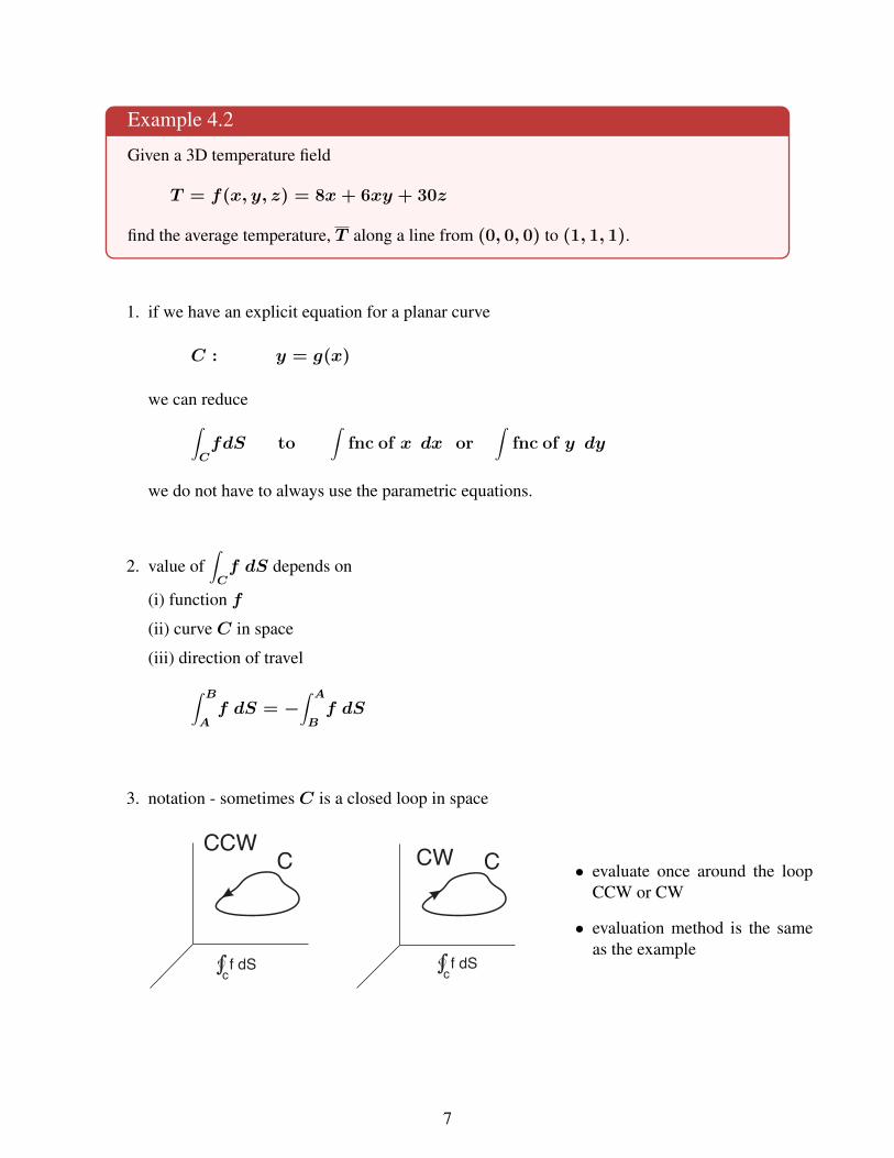
3. notation - sometimes C is a closed loop in space

CCWCWC C

f dS f dSc c

• evaluate once around the loopCCW or CW

• evaluation method is the sameas the example

7

Example: 4.3a

Suppose the temperature near the floor of a room (say at z = 1) is described by

T = f(x, y) = 20−x2 + y2

3where −5 ≤ x ≤ 5

−4 ≤ y ≤ 4

What is the average temperature along the straight line path fromA(0, 0) toB(4, 3).

Example: 4.3b

What is the average room temperature along the walls of the room?

T =

∮Cf(x, y)dS∮CdS

where the closed curve C is defined in 4 sections

C1 y = −4 x = t −5 ≤ t ≤ 5

C2 x = 5 y = t −4 ≤ t ≤ 4

C3 y = 4 x = 5− t 0 ≤ t ≤ 10

C4 x = −5 y = 8− t 0 ≤ t ≤ 8

Example: 4.3c

What is the average temperature around a closed circular path→ x2 + y2 = 9?

where C is a closed circular path

T =

∮Cf(x, y)dS∮CdS

where x(t) = 3 cos t

y(t) = 3 sin t

for 0 ≤ t ≤ 2π.

8

Line Integrals of Vector Functions

ReadingTrim 14.3−→ Line Integrals Involving Vector Functions

14.4−→ Independence of Path

Assignmentweb page−→ assignment #10

Let’s examine work or energy in a force field.

W = ~F · ~d

Now consider a particle moving along a curve C is a 3D force field.

W =∫C

~F (x, y, z)︸ ︷︷ ︸force value evaluated along C

· d~r︸︷︷︸displacement along C

(1)

This is a line integral of the vector ~F along the curve C in 3D space.

In component form:

~F = iP + jQ+ kR

d~r = idx+ jdy + kdz

W =∫CPdx+Qdy +Rdz (2)

Equations (1) and (2) are equivalent.

Use the equation of curve C (either in an explicit form, i.e. y = f(x) etc., or in a parametric

form) to reduce (2) to∫ αt=0g(t)dt or

∫ βx=n

h(x)dx etc.

Example 4.4

Given a force field in 3D:

~F = i(3x2 − 6yx) + j(2y + 3xz) + k(1− 4xyz2)

What is the work done by ~F on a particle (i.e. energy added to the particle) if it moves in astraight line from (0, 0, 0) to (1, 1, 1) through the force field.

9

Notes

1. If we have an explicit equation for the curve, we can sometimes reduce to a form∫

(fnc of x) dx

etc. There is no need for parametric equations.

2. The work termW can be either +’ve or -’ve.

In a +’ve form,∫~F and

∫d~r, are in the same direction, where the work done by the force

energy is added to the object by ~F .

In the -’ve form, ~F opposes the displacement. The energy is removed from the object.

+’veW =∫C~F · d~r

3. closed path notation

W =∮CCW

~F · d~r once CCW around loop

W =∮CW

~F · d~r once CW around loop

4. A special case is the conservative force field

∮~F · d~r = 0

We know that∇× ~F = 0. There is no work in a closed loop.

We also know that∇φ = F , which is integrated gives

∫C

~F · d~r = φ1 − φ2

Therefore for a conservative force field, the work is a function of the end points not the path.

This is the same for any C connecting the same 2 end points.

W is always the same number if ~F is conservative.

10

Example: 4.5a

The gravitational force on a mass,m, due to mass,M , at the origin is

~F = −GMm~r

|~r|3= −K

~r

|~r|3where K = GMm

The vector field is given by:

~F (x, y, z) = iP + jQ+ kR where P = −Kx

(x2 + y2 + z2)3/2

Q = −Ky

(x2 + y2 + z2)3/2

R = −Kz

(x2 + y2 + z2)3/2

Compute the work, W , if the mass, m moves from A to B along a semi-circular path inthe (y, z) plane:

y2 + z2 = 16y or z =√

16y − y2 and x = 0

From A(0, 0.1, 1.261) toB(0, 16, 0)

A B

x

y

M

z

m

curve C in the x=0 plane

(xz plane) - circle, radius 8

center (0,8,0)

Example: 4.5b

Find the work to move through the same field, but following a straight line path fromA(0, 0.1, 1.261) toB(0, 16, 0).

A

B

x

y

M

zm curve C

11

Conservative Force Fields

ReadingTrim 14.5−→ Energy and Conservative Force Fields

Assignmentweb page−→ assignment #10

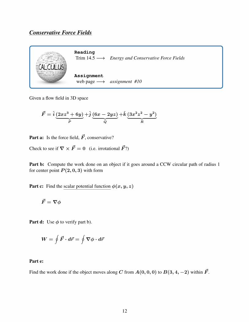
Given a flow field in 3D space

~F = i (2xz3 + 6y)︸ ︷︷ ︸P

+j (6x− 2yz)︸ ︷︷ ︸Q

+k (3x2z2 − y2)︸ ︷︷ ︸R

Part a: Is the force field, ~F , conservative?

Check to see if∇× ~F = 0 (i.e. irrotational ~F ?)

Part b: Compute the work done on an object if it goes around a CCW circular path of radius 1for center point P (2, 0, 3) with form

Part c: Find the scalar potential function φ(x, y, z)

~F = ∇φ

Part d: Use φ to verify part b).

W =∮~F · d~r =

∮∇φ · d~r

Part e:

Find the work done if the object moves along C fromA(0, 0, 0) toB(3, 4,−2) within ~F .

12

Surface Integrals of Scalar Functions

ReadingTrim 14.7−→ Surface Integrals

Assignmentweb page−→ assignment #11

x

y

zsurface z=g(x,y)

surface area dS

dA = dx dyprojection

xyprojection in (x,y) plane

surface area of z = g(x, y)

S =∫ ∫Rxy

√√√√1 +

(∂g

∂x

)2

+

(∂g

∂y

)2

dxdy

Now suppose the surface z = g(x, y) iswithin a 3D temperature field

T = f(x, y, z)

What is the average temperature measured over the surface z = g(x, y)?

Add up T for each dS area element and divide by the total area of S to get the average.

T =

∫ ∫Sf(x, y, z)dS

Area of S

The numerator is called the surface integral of f(x, y, z) over the surface S (i.e. z = g(x, y)).

To evaluate

∫ ∫SfdS =

∫ ∫Rxy

f [x, y, g(x, y)]︸ ︷︷ ︸T values on the surface

√√√√1 +

(∂g

∂x

)2

+

(∂g

∂y

)2

dxdy︸ ︷︷ ︸dS area element

This becomes

∫ ∫Rxy

F (x, y)dxdy

13

Notes

1. sometimes it is easier if we switch to polar coordinates

∫ ∫Rxy

F (x, y)dxdy →∫ ∫Rxy

H(r, θ)rdrdθ

where x = r cos θ and y = r sin θ.

2. notation = we have a closed surface in space, i.e. a sphere surface

g(x, y)→ z =√a2 − x2 − y2

∮ ∮Sf(x, y, z)dS

Example: 4.6

Suppose the temperature variation (same for all (x, y)) in the atmosphere near the groundis

T (z) = 40−z2

5

where T is in ◦C and z is inm. Look at a cylindrical building roof as follows:

x

z

30 m long

10 m high

10 m

What is the air temperature in contact with the roof?

14

Surface Integrals of Vector Functions

ReadingTrim 14.8−→ Surface Integrals Involving Vector Fields

Assignmentweb page−→ assignment #11

Given a full 3D velocity field, ~V (x, y, z) in space (i.e. air flow in a room).

Given some surface z = g(x, y) within the flow→ calculate the flow rate Q (m3/s) crossingthe surface S, we can write G = z − g(x, y), where G is a constant since the surface is a levelsurface or a contour.

dS at (x,y,z)

surface z=g(x,y)

or

G(x,y,z) = z - g(x,y) = 0

V

The basic idea is to consider the element dS of the surface at some arbitrary (x, y, z). Thencompute the unit normal vector to dS

n = (±)∇G|∇G|

This will vary over S. The (±) will be controlled by the direction of the flow.

The flow across dS is (~V · n)︸ ︷︷ ︸component normal to surface

dS.

Add up over all dS elements to get the total flow across the surface

Q =∫ ∫

S

~V · n dS

15

This is called the surface integral of the vector field ~V over the surface S defined byz = g(x, y).

The actual evaluation is similar to the last example.

• ~V · n will end up giving some integrand function f

• project dS onto (x, y) plane

dS =

√√√√1 +

(∂g

∂x

)2

+

(∂g

∂y

)2

dxdy

Q =∫ ∫Rx,y

f(x, y)

√√√√1 +

(∂g

∂x

)2

+

(∂g

∂y

)2

dxdy

• then proceed as before.

Example: 4.7

Given a velocity field in 3D space

~V = i(2x+ z) + j(x2y) + k(xz) find

a) the flow rateQ (m3/s) across the surface z = 1 for0 ≤ x ≤ 1 and 0 ≤ y ≤ 1 in the +’ve z direction

b) the average velocity across the surface

z

x

y

1

1

1

xy

dSsurface S

16

Integral Theorems Involving Vector Functions

We will examine vector functions in 3D:

Force Field: ~F (x, y, z) = iP + jQ+ kR

Vector Field: ~V (x, y, z) = iu+ jv + kw

We have defined 2 types of integrals for such functions.

Line Integrals

z

y

x

C

F

∫C

~F · d~r =∫CPdx+Qdy +Rdz

This can be interpreted as work done by ~F field onan object that moves along C within the field.

Surface Integrals

z

y

x

S

V

∫ ∫S

~V · n dS

This can be interpreted as the flow across surface Sin the n direction due to the ~V field.

There are three theorems which state identities involving these types of integrals.

17

1. Divergence Theorem

z

y

x

V field in 3D space

closed surface S enclosing

volume (on RHS)

Also called Green’s theorem in space - this is the 2ndvector form of Green’s theorem.

∮ ∮S

~V · ~n dS =∫ ∫ ∫

V(∇ · ~V )dV

where

~V = velocity field

V = volume

2. Stokes TheoremAlso called 1st vector from of Green’stheorem.

∮C

~F · d~r =∫ ∫

S(∇× ~F ) · n dS

where the surface S is any surface in 3D withC as a boundary.

x

y

z

C

F defined in 3D space

closed curve C

in 3D space

3. Greens Theorem

This is essentially a 2D statement of Stoke’s the-orem, where in 2D

~F = iP + jQ

∇× ~F = k

(∂Q

∂x−∂P

∂y

)x

yC

F defined in 2D space

∮CPdx+Qdy =

∫ ∫R

(∂Q

∂x−∂P

∂y

)dxdy

18

Divergence Theorem

ReadingTrim 14.9−→ The Divergence Theorem

Assignmentweb page−→ assignment #11

Trim in section 14.9 has a detailed proof of the Divergence Theorem. They try to interpret themeaning of

∮ ∮S

~V · ndS =∫ ∫ ∫

V(∇ · ~V )dV

This equation applies for any vector function ~V , but is used most for velocity fields in fluids. Whenwe consider ~V , the theorem concerns net outflow to inflow (m3/s) for a region in space (like asphere).

The left side of the equation is a surface integral of V over a closed surface, S in 3-D space withn being the outward normal to each dS.

We recall that ~V · ndS gives the flow rate (m3/s). When we add this up over the entire surface(as in the LHS of the equation) we obtain the net flow rate crossing the closed surface.

i.e.

net outward flow(m3/s)− net inward flow(m3/s)

The right hand side of the equation is a calculation of ∇ · ~V for each differential volume, dVinside the surface S. We then add them all up.

For the differential volume, V

inflow (m3/s) = u(x) · area+ v(y)(∆x)(∆z)

outflow (m3/s) = u(x+ ∆x) · (∆y)(∆z) + v(y + ∆y)(∆x)(∆z)

The net flow is then

outflow − inflow = (∆x)(∆y)(∆z)

[u(x+ ∆x)− u(x)

∆x+v(y + ∆y)− v(y)

∆y

]

19

= (dV)

(∂u

∂x+∂v

∂y

)

= (∇ · ~V )dV

Therefore the RHS (∇ · ~V )dV gives the net outflow minus inflow for a volume element dV .

The integral∫ ∫ ∫

V , adds up the differential flow for all volume elements, dV inside of surface S.There is a cancellation of terms because the outflow from one ∆V becomes the inflow to the nextvolume.

When we sum over all ∆V , we are left with the difference between the inflow and the outflow atthe boundaries of the volume.

∮ ∮S

~V · ~ndS =∫ ∫ ∫

V(∇ · ~V )dV

outflow − inflow(m3/s) triple sum of all outflow − inflow

across boundary surface for ∆V volumes inside

S of volume V in 3D space the volume V in 3D space

Example: 4.8

Given

~V = i(1 + x) + j(1 + y2) + k(1 + z3)

verify the divergence theorem for a cube, where 0 ≤ x, y, z ≤ 1 i.e. show that∮ ∮S

~V · ndS =∫ ∫ ∫

V(∇ · ~V )dV

where

S = cube surface (closed)V = interior volume of the cube

20

Stoke’s Theorem

ReadingTrim 14.10−→ Stoke’s Theorem

Assignmentweb page−→ assignment #11

The formal proof is offered in Trim 14.10.

∮C

~F · d~r =∫ ∫

S(∇× ~F ) · n dS

This has a similar meaning to Green’s theorem but now in 3D space instead of a plane.

x

y

z

C

F

~F (x, y, z) is a 3D force field. The LHS of the equa-tions is the work done when the object moves oncein a CCW direction along the path C in 3D.The RHS is the work computed over a surface inte-gral

∫ ∫S .

Like Greens theorem, it works because of the interior cancellations of work, when we move arounda surface element dS inside C.

Note: the unit normal, n for the LHS is based on a right hand rule as follows.

dS

dS

dS

n

n

n

C

any surface S in 3D

with C as the boundary

if CCW on C

if CW on C

^

^

^

The work on all internal surfaces cancel, leaving only the surface work in the CCW direction.

21

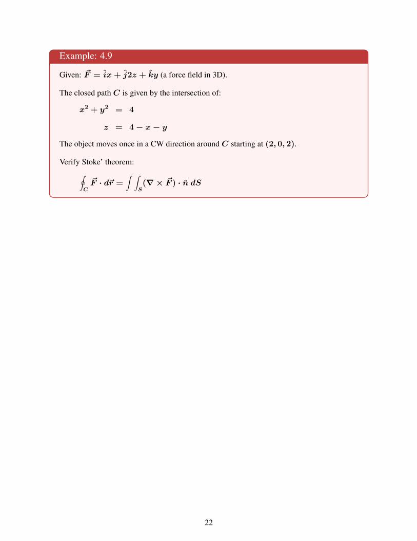
Example: 4.9

Given: ~F = ix+ j2z + ky (a force field in 3D).

The closed path C is given by the intersection of:

x2 + y2 = 4

z = 4− x− y

The object moves once in a CW direction around C starting at (2, 0, 2).

Verify Stoke’ theorem:∮C

~F · d~r =∫ ∫

S(∇× ~F ) · n dS

22

Green’s Theorem

ReadingTrim 14.6−→ Green’s Theorem

Assignmentweb page−→ assignment #10

The theorem involves work done on an ob-ject by a 2D force field. The 2D force fieldis given by

F (x, y) = iP (x, y) + jQ(x, y) x

y

P

Q F

C

We will examine an object that moves once CCW around a loop in ~F . The region inside the loop isdefined asR. The normal vector for the regionR is k (outwards) to the right for a CCW motionof C. The theorem states

∮CPdx+Qdy =

∫ ∫R

(∂Q

∂x−∂P

∂y

)dxdy

The left hand side of the equation,∮C

~F · d~r in 2D

is the work done by the field ~F on the object as itmoves on C. This consists of force times distancefor each d~r added up over C.

F

dr

The right hand side of the equation,∫ ∫R

(∇× ~F )·

kdxdy in 2D gives the direction of travel on C forthe work given by the LHS. Maps movement of anelement ∆x∆y as it moves around fromA toA.

x

y

P

Q F

x x + x

y + y

y A

k^

out

23

The force component times the distance for each sidegives the work done. Q

P

Q

P

at x+ x

at y+ y

at x

at y

A

Work = Q|at x+∆x ∆y − P |at y+∆y ∆x− Q|at x ∆y + P |at y ∆x

= (∆x∆y)

[Q|at x+∆x − Q|at x

∆x−P |at y+∆y − P |at y

∆y

]

In the limit, the work done by ~F to move the object CCW around dxdy area is

(∂Q

∂x−∂P

∂y

)dxdy

Now we can sum up for all dxdy elements inside C.

There are some cancellations (+) (-) for all interior ∆x,∆y paths. Therefore when we do∮ ∮R

,we are left with the work terms on the boundaries ofR.

∮CPdx+Qdy =

∫ ∫R

(∂Q

∂x−∂P

∂y

)dxdy

work when we sum of all work if

move once CCW around move once CCW around all

boundary curve C (dxdy) area elements of R

inside C

24

Example: 4.10

Given a 2D force field, ~F (x, y) = i(xy3) + j(x2y) and a path C in the field:

Verify Green’s theorem

∮CPdx+Qdy =

∫ ∫R

(∂Q

∂x−∂P

∂y

)dxdy

with

P = xy3

Q = x2y

25