Vegetation Classification Using Hyperspectral Images

Fengjunyan Li, Kazim Ergun, Osman Cihan Kilinc, Yuming Qiao

Abstract— Every object has its unique spectral ’signature’over the electromagnetic spectrum, and this can be capturedusing hyperspectral sensors. In this project, we use thesesignatures for discriminating different types of plants. It hasbeen shown that machine learning algorithms are very powerfulat learning patterns. They have already been utilized for clas-sification tasks in various fields. Indian pines dataset1 is usedfor testing and other measurements. Treating the hyperspectralbands in the images as features and each pixel as a sample,we classify plants with convolutional neural networks(CNN)and support vector machines(SVM). Furthermore, we optimizeCNN to prevent overfitting, accelerate inference, and reducethe resources it uses with respect to memory, battery andcomputational power. The results demonstrate that CNN is verysuccessful in hyperspectral image classification tasks and opti-mizations further increase its accuracy. We achieved 83.9% testaccuracy using SVM with Polynomial kernel, and successfullyachieved 99.2% with CNN.

I. INTRODUCTION

Hyperspectral imaging, like other spectral imaging, col-lects and processes information across the electromagneticspectrum, usually in visible, near infrared, and short-waveinfrared wavelengths. Recently, with the development ofhyperspectral sensors, it has become possible to go beyondtraditional RGB images and capture hundreds of spectralbands sampled with narrow wavelength intervals. There-fore, taking advantage of contiguous narrow bands, thesehyperspectral sensors enabled the study of the chemicalproperties of scene materials remotely for the purpose ofidentification, detection, and chemical composition analysisof objects in the environment. Hence, hyperspectral imagescaptured from earth observing satellites and aircraft havebeen increasingly important in agriculture, environmentalmonitoring, and urban planning.

The fundamentals of hyperspectral imaging are basedprimarily on the interaction of light with matter. When aphoton is incident on a surface of a medium, energy canbe absorbed, transmitted and/or reflected by that surface,with a wavelength dependency determined by the materialproperties. The ratio of the energy reflected or scattered bythe surface to the incident energy is termed as the reflectance,and measured by the hyperspectral sensors. For a particularobject, the reflectance spectrum shows characteristic bandsinduced by the constituent materials. Therefore, spectral re-flectance provides substantial information about the materialproperties.

All authors are graduate students in University of California San Diego,Electrical and Computer Engineering

(a) Hyperspectral Images (b) Satellite Image of In-dian Pines

Fig. 1: Hyperspectral Images and Indian Pines Dataset

In this project, we utilize the spectral reflectance infor-mation to classify plant types as an application of precisionagriculture. Specifically, we use hyperspectral images cap-tured from satellites and use machine learning techniquesto discriminate crops in a plantation area. We use IndianPines Hyperspectral Dataset1 gathered by AVIRIS Sensor.For classification, we have used Convolutional Neural Net-works(CNN)2 and Support Vector Machines(SVM) with di-mensonality reduction methods Principle Component Anal-ysis(PCA) and Nonnegative Matrix Factorization(NMF). Inshort, the input to our algorithm is an a hyperspectral imagewith size 145×145×224 seen in figure 1 (b). We then use aSVM and CNN model to output a predicted vegetation classfor each pixel.

II. RELATED WORK

In their work Delalieux et al.3 used hyperspectral data todetect apple scab caused by disease. The study involved theidentification of infected trees and selection of wavelengthsbest suited for classifying the infected leaves from those ofthe healthy leaves. The spectral data were analyzed usingmethods as LDA, logistic regression analysis (for each wave-length), partial least squares logistic discriminant analysis,and tree-based modeling for classifying the infected leavesclassification.

Lee et al.4 worked on the detection of greening in citrusplantation using hyperspectral images. He used the spectralangle mapping and spectral feature fitting classification tech-niques. However, the author was not able to achieve highclassification accuracies due to a large variability within thedata.

Begum Demir and Sarp Erturk5 used Relevance VectorMachine. They propose that RVM has similar strategy withSVM but require fewer relevance vectors. With lower com-plexity, RVM can achieve similar classification as SVM. Inthe paper of G. Mercier and M. Lennon,6 they researched

SVM with spectral-based kernel to classify satellite hyper-spectral images. Their method is able to reduce the falsealarm by traditional kernel. We will try to use traditionalkernels in the SVM of our project to verify the result.

In their work Makantasis et al.2 show that using CNN,hyperspectral images can be successfully classified. CNNcan encode the spectral and spatial features of pixel. Thelow-to-high hierarchy of features improve the performance ofclassification greatly. In our CNN implementation we extendand optimize their method with layer pruning and layercompression methods. Although these methods are widelyadopted in the industry and research, to our knowledge noother work has been published that applies such optimiza-tions on top of the model Makantasis et al. provided in theirwork.

III. DATASET FEATURES AND PREPROCESSING

The dataset Indian Pines1 consists of 145× 145 pixelsand 224 spectral reflectance bands in the wavelength range0.4−2.5 µm. There are 16 classes, some of them being fromthe same crop type but at different stages of growth. Interms of machine learning, each pixel in the images arelabeled according to their class and contain 224 features.Plainly speaking, each pixel represents a location, and thatlocation contains 224 spectral bands. For example, the firstfive spectral bands of a pixel/location can have values suchas : 3172, 4142, 4506, 4279, 4782. Data is preprocessedfor four reasons: (i) to introduce variability into data, (ii) tostrengthen the weak classes, (iii) to reduce the dimensionalityof the feature set and (iv) to prepare data for processing.

A. Oversampling

In Indian Pines dataset, there is a huge imbalance betweenthe number of samples of different crop types. For example,as shown in Table I. There are 20 Oats samples whereasthe number of Soybean-mintill samples are 2455. To fixthis imbalance issue, we oversampled the classes which hassubstantially less number of samples compared to the others.Without oversampling, the classifier would give more weighttowards the classes with high number of samples, whichwould lead to misclassification in minority classes. In ourimplementation, we check the number of samples(pixels)per each class and for each class we concatenate samplesfrom that class to data matrix to make up for the differencebetween classes. Later, we randomly redistribute samples inthe dataset.

B. Data Augmentation

To prevent overfitting and train our model for the realworld, where images can come with different rotations anddifferent angles, we introduce new data by augmenting theexisting data. This increases the variability of data andprevents overfitting. Hence, it increases the accuracy. Thisachieved by flipping and rotating the images. In our imple-mentation we randomly choose either to flip left-right, up-down or rotate each sample.

TABLE I: 16 Classes of Indian Pines Dataset.

Class # of Samples

Alfalfa 46Corn-notill 1428Corn-mintill 830Corn 237Grass-pasture 483Grass-trees 730Grass-pasture-mowed 28Hay-windrowed 478Oats 20Soybean-notill 972Soybean-mintill 2455Soybean-clean 593Wheat 205Woods 1265Buildings-Grass-Trees-Drives 386Stone-Steel-Towers 93

C. Dimensionality Reduction

Hyperspectral data is large in size, since information fromwhole spectrum range is included in a pixel. However, notall the information contained in the data is relevant for theanalysis, thus can be discarded without much loss. Moreover,a lot of the bands shows high correlation. Applying dimen-sionality reduction on our data before classification step helpsus reduce the processing time by projecting the data on asmaller sized space without loss of information.

1) Principal Component Analysis: Principal componentanalysis (PCA) is a statistical procedure that uses an or-thogonal transformation to convert a set of observations ofpossibly correlated variables into a set of values of linearlyuncorrelated variables called principal components. Thistransformation is defined in such a way that the first principalcomponent has the largest possible variance (that is, accountsfor as much of the variability in the data as possible),and each succeeding component in turn has the highestvariance possible under the constraint that it is orthogonalto the preceding components. The resulting vectors are anuncorrelated orthogonal basis set. More information aboutPCA can be found in.7 To show the amount of informationkept after dimension reduction, we plotted the variance ratiofor different number of principle components in Figure2. Wetook the 30 top principle components since it is enough toexplain the 0.99 of the total variance.

Fig. 2: Variance Explained vs Number of Principle Compo-nents

Using the results of the PCA method, we can writeAxi = λixi , where xi are the eigenvectors of A, λi are theeigenvalues of A, for any matrix A.

For data given as a set of m vectors ∈Rn, x1, ...,xm,PCAmethod can be formalized as an optimization problem asfollows:8

maximizeW∈Rm×k

||XW||2F

subject to ||W||= 1,

where X denotes the normalized covariance matrix X =1m ∑

mi=1 xixT

i and W is the orthogonal projection matrix.2) Nonnegative Matrix Factorization: Nonnegative Ma-

trix Factorization (NMF) is a matrix factorization methodwhere a matrix V is factorized into matrices W and H,with the property that all three matrices have no negativeelements. Similar to PCA, we use NMF as a tool to reducedimensionality. Difference between PCA and NMF is thatwhile PCA has negative elements, the most rule of NMFis that it does not have any negative elements. Thus, withrespect to PCA, NMF has more floating point elements toapproximate the matrix as close as possible to the original.A comparison with respect to accuracy between PCA andNMF is provided in the results section. The standard NMFproblem can be formulated as follows:

minimizeW∈Rm×r ,H∈Rr×n

||V−WH||

subject to W,H≥ 0,

IV. CLASSIFICATION METHODS

A. Support Vector Machines

Support Vector Machine, also known as SVM, is popularfor solving problems about classification, detection and re-gression. In support vector machine, the model constructs ahyperplane or set of hyperplane in higher dimension space.From,9 we can know the structure of SVM. The hyperplanelinear model of SVM can be defined as

y = wTφ(x)+b

where φ(x) is transformed feature space. The margin isdefined as the smallest distance from the decision hyperplaneto the closest point from dataset. In the SVM problem, weare trying to construct the decision boundary hyperplane tomaximize the margin with dataset. For each data point, ti isthe target label, where t∈ {1,−1}. In our case, the problemis not linearly separable, we will use soft-margin SVM andintroduce slack variable ξi≥ 0. ξ allows the misclassificationof outline. When ξi > 1, the data point is misclassified. At thesame time, we should have inequality constraint as follows:

ti(wTi φi(x)+b)≥ 1−ξi

This is because we need to make y(xn)> 0 for those pointsthat have tn = 1, and make y(xn) < 0 for those points that

have tn =−1. The distance from data point xn to the decisionboundary in hard-margin is given by:

tny(xn)

||w||=

ti(wT φ(x)+b)||w||

In order to find the maximum margin solution, we solve thefollowing problem:

argmaxw,b1||w||

minn(tn(wTφ(x)+b)

With simplification of problem and the soft-margin slackvariable , the SVM problem eventually becomes:

argmaxw,b,ξ12||w||2 +C

N

∑n=1

ξn

s.t tn(wTφ(x)+b)≥ 1−ξn;ξn ≥ 0;n = 1,2, ...,N

The variable C is the regularization parameter to control thetradeoff between margin and the tolerance of misclassifi-cation. In addition,in the dataset is non-linearly separable,we can use kernel trick to transform them to higher lineardimension, such as Gaussian Kernel. Since the SVM problemis a convex optimization problem, we can always obtain aglobal optimum from the model. With the optimal decisionboundary, we can use it to classify our dataset into differentlabels.

B. Convolutional Neural Networks

With the development in hardware technology, convo-lutional neural networks have become popular for imageclassification tasks in the recent years. In convolutionalneural networks, the first few hidden layers are convolutionallayers. The convolutional layers consist of spatially smallfilters. These filters are applied through a sliding-windowacross the input. Each filter outputs an activation map in2-D that corresponds to an edge, rotation, or some otherhidden feature of the input. These activation maps are thenaggregated to be the output of that convolutional layer.The key difference of convolutional layers is that they areconnected only to a local region of the input volume. Despiteof the skepticism CNN received at first,it has been provenby countless papers and against many benchmarks that CNNis actually a very powerful method for image classification.Thus, it was adopted by many researchers in various fieldsfor different tasks.

1) Architecture: Our architecture is similar to the genericConvolutional Neural Network architecture, which usuallyconsists of convolutional layers, followed by pooling layers,normalization layers and finally the fully connected layers.However, we do not use pooling layers. Although they areusually useful and it is counterintuitive to not use them,pooling layer actually decreases the accuracy in our case.Thus we did not use them. During forward propagation, theequation below is calculated at each neuron. Suppose thatthis neuron has m connections in the previous layer, theseconnections have weights wi and the activation values of the

units are ai.m

∑i=1

wiai +b

The output of this calculation then goes through a non-linear function. We use ReLu as our non-linear activationfunction, which clamps the negative activations to 0 anddropout method to provide some relief from overfitting. TheReLu function can be mathematically represented as:

f (x) = max{0,x}

Since the gradient of a cost function with respect to itsparameters gives the direction of gradient ascent, to minimizethe cost function we need to go in the opposite direction.Then, we simply leverage the chain rule and derivatives toupdate the parameters during backpropagation.

C. Optimizations

One of the problems that should be addressed is theresources neural networks use, since they are a drain onthe resources. They are computationally expensive to use.They require a large memory, a powerful battery and apowerful GPU. Therefore, today much of the computationis done via the cloud services. However, recent innovationsshow that machine learning will become ubiquitious. Edgedevices traditionally operate on low resources. Moreover,drones also play an important part in precision agricultureand agricultural technology. We can leverage hyperspectralimaging technology on the drones to provide farmers a realtime feedback. Thus, it is important to make neural networkslight enough to put them on edge devices.

By optimizating our neural networks, we reduce thenumber of parameters and computations. Thus, we acce-larate inference and decrease the resource requirements. Forthis reason, we have implemented two methods: (i) layercompression and (ii) layer pruning. Although most of thecomputation is typically done on convolutional layers, fullyconnected layers have the most connections and parameterson the convolutional neural networks. Thus, we have imple-mented these methods on fully connected layers.

1) Fully Connected Layer Compression: Layer compres-sion is used to reduce the number of parameters of a layer.It is usually achieved by decomposing the weight matrixof a layer and then replacing that matrix with a low rankrepresentation or approximation. This method provides adramatic decrease in the number of parameters.

We replaced only the first fully connected layer by its de-composition, preserving all other layers in the network. First,we used PCA to select the number of principal componentsthat can successfully approximate its weight matrix. Then,we used singular value decomposition to factorize the matrixand replaced this layer with its factorization.

Since each neuron is connected to all neurons in theprevious layer, if there are m neurons in the previous layerand n neurons in that layer, then there are mxn connections.Suppose we want to replace the weight matrix W ∈ IRmxn

with low rank approximation of rank k. The singular valuedecomposition of W is below.

W = USVT , where U ∈ IRm×m,S ∈ IRm×n and V ∈ IRn×n

After selecting the first k principal components of the matrix,we use only U ∈ IRmxk,S ∈ IRk×k and V ∈ IRk×n. Thus, thematrix W is replaced by matrices R1∈ IRm×k and R2∈ IRk×n.

R1 = Um×kSk×k,

R2 = VTk×n,

where R1 and R2 give the low-rank approximation of theoriginal weight matrix W. We replace the first fully con-nected layer with two new fully connected layers, constructedfrom R1 and R2, respectively. While the first replacementlayer does not have any bias assigned, the second replace-ment layer is assigned the bias of the original layer. Thus, wereduce the number of parameters in the matrix from m× nto k× (m+ n). The change in the number of parameters isdramatic, the results are demonstrated in the results section.

2) Fully Connected Layer Pruning: Layer pruning isanother method to optimize the neural networks. The ideais based on reducing the number of connections betweenthe layers. We used a threshold based method, where wemasked the connections with respect to the absolute valueof their weights. The masked weights are not trained duringtraining can be completely cut-off during deployment withcomplementary methods.

D. Noise Reduction

The noise reduction was done after the result of SVMand neural networks. As we inspected the resulting im-age, we found that there were always some dangling mis-classifications points. We did the noise reduction by correct-ing points ,whose neighbors all belonged to another singleclass, to his neighbor class. We believe that it is impossiblefor a plant to grow while all the plants near it belonged toanother class, and the noise reduction result proved that ourbelief is correct.

E. Implementation

We used Keras 2.1.510 in conjunction with Tensorflow11

1.7.0. Keras is an open source maintained by mostly peo-ple from Google, where one can quickly prototype neuralnetworks. Nvidia GTX 1070 graphics processing unit wasused with CUDA 9.012 for calculations. The developmentwas completed on a Windows 10 computer. The modularityof the code was also key aspect of the development.

Other libraries include spectral, matplotlib,13 numpy,14

scipy.15learn for utilities such as plots, and training-testdataset splitting and image outputs.

We used Adam for gradient descent optimization with alearning rate of 0.0001 and a decay of 1e−6. Adam acts like aball with friction that goes down the convex curve of the lossfunction. To achieve that in addition to storing exponentiallydecaying average of past squared gradients, it also keeps anexponentially decaying average of gradients and computes anadaptive learning rate for each parameter. Given the 6 GB

RAM of Nvidia GTX 1070, the minibatch size was selectedto be 100. This assured the best performance/accuracy forthe model.

V. RESULTS

We split our dataset to training and test datasets, %75 and%25, respectively. For CNN, we have included the vanillaclassifications (without any optimizations) with PCA-appliedand NMF-applied input. With PCA-applied input, our modelgives a higher accuracy compared to NMF-applied input.Later, we used the model trained with the PCA-applied dataas a baseline and applied our optimizations on top of thatmodel. In this section, we make several comparisons such asretraining and not retraining the model after optimizations.We also demonstrate the results with different ratios ofnetwork pruning and different ratios of layer compression.The best accuracies we obtained without denoising are givenin the table below.

CNN VanillaClassification with

PCA-Input

CNN withNetwork

Compression

CNN with LayerPruning

%98.1 %99.1 %98.5

TABLE II: Best Accuracies Obtained using CNN

For SVM, the best accuracies we obtained without denois-ing are given in the table below.

SVM Gaussian Kernel SVM Polynomial Kernel%80.7 %82.7

TABLE III: Best Accuracies Obtained for SVM Kernels

The final accuracies we obtained with best CNN and bestSVM after denoising are given in the table below.

CNN with NetworkCompression

SVM Polynomial Kernel

%99.2 %83.9

TABLE IV: Final Accuracies after Noise Reduction

A. Support Vector Machines

We provide a detailed explanation of our results, graphsand output images. We have only used Indian Pines datasetas a benchmark. We used %25 of the dataset as the test setand the rest was used as the training set. The operationswere completed on the preprocessed data as explained in thepreprocessing section.

1) Gaussian Kernel: We start by choosing Gaussian Ker-nel. The training error is 87.8%, and the testing error is80.7%. Figure 3 is the resulting classified image. It can beseen that the resulting image successfully shows the structureof the plantation, but there are also many misclassificationpoints. Some classes are well learned but some still needmore training.

2) Polynomial Kernel: The best result we can get isfrom order = 3. The training accuracy for the polynomialkernel is 93.4%, and the testing accuracy is 82.7%. Thetesting accuracy is better than the Gaussian Kernel. Figure 3shows the resulting classified image. It can be seen that thePolynomial kernel model has a better result with much lessmisclassified points.

(a) Gaussian Kernel (b) Polynomial Kernel

Fig. 3: Support Vector Machine Classification

B. Convolutional Neural Networks

We provide a detailed explanation of our results, graphsand output images. We have only used Indian Pines datasetas a benchmark. We used %25 of the dataset as the test setand the rest was used as the training set. The operationswere completed on the preprocessed data as explained in thepreprocessing section.

1) Vanilla Classification:

1) PCAWe implemented two different methods for dimen-sionality reduction. As explained in the preprocessingsection, the input can be successfully approximatedby using only the first 35 principal components. Thefigure 4 shows our results with no optimizations giventhe first 35 principal components. Learning curve con-verges around %98.1 accuracy.

2) NMFThe first 35 components of the nonnegative matrixfactorization was used to make a fair comparison withPCA. However, it can be seen from figure 4 belowthat compared to PCA, NMF produces a poorer result(%95.67 accuracy). This might be due to the factthat NMF does not have negative values, thus eachof its components also include very small floatingpoint numbers. During training, this might engenderan increased number of errors in calculations due tofloating point overflow.

(a) PCA-applied Data Learning Curve (b) NMF-applied Data Learning Curve

Fig. 4: Learning Curves of Vanilla Classifications

It is clearer from figure 5 that even without anyoptimizations the classification with the PCA-appliedinput is better than the NMF-applied input.

(a) PCA Vanilla Classi-fication

(b) NMF Vanilla Classi-fication

Fig. 5: Vanilla Classifications

2) Fully Connected Layer Compression: Using the trainedmodel of the PCA vanilla classification, we took the weightof the first fully connected layer and displayed its principalcomponents. The figure below shows that it is nearly linear.Thus, this means that all the dimension of the weight matrixis nearly equally important.

q

Fig. 6: PCA of the First Fully Connected Layer

The reduction in the number of parameters is clearer inthe figure below. The first fully connected layer has m× nparameters. Table VI shows how small it gets with differentlow-rank representations. Even though we significantly de-crease the number of parameters, we get acceptable results.

Interestingly, even without retraining there is an increasein accuracy after layer compression. Figure 7 shows that evenfor very low rank factorizations, we achieve higher accuracyor only a negligible decrease in accuracy. In our case layercompression perturbs the network and prevents overfitting.When k=75, the model peaks at %99.1 accuracy. Moreover,it can be observed that the retraining of the network does

little to increase the accuracy. This is because we closelyapproximate the weight matrix and it is not always necessaryto retrain the network after compression.

(a) Without Retraining (b) With Retraining

Fig. 7: Layer Compression: Accuracy vs Rank

3) Fully Connected Layer Pruning: We pruned all thefully connected layers with some ratio k. Only the largest%k of the weights was kept, while the others were clampedto 0. Thus, while the original model had 2430×180+180×16 parameters, this goes down dramatically with pruning.The subsequent reductions are clear in table VI. It canbe observed from figure 8 that even without training, thismethod preserves and slightly increases the accuracy ofour model to %98.2, but as k grows the accuracy slowlydecreases. However, after %90 of the weights are prunedthe accuracy drops significantly. Results are encouraging.Similar to compression pruning works as a complement andprevents overfitting. The accuracy slightly increases as kgrows to %60 pruning at %98.5. The difference betweenretraining and not retraining is clear. While the accuracydrops after %80 percent pruning with the untrained model,the accuracy is relatively preserved until %95 pruning in theretrain model. Moreover, this method is orthogonal to layercompression and can be used in conjunction.

(a) Without Retraining (b) With Retraining

Fig. 8: Uniform Pruning: Accuracy vs Pruning Ratio

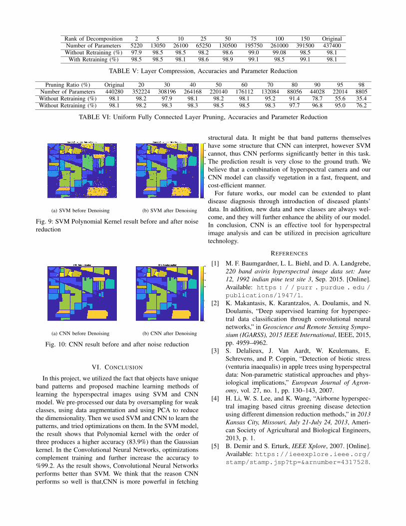
4) Noise Reduction: We run the noise reduction based onour SVM/CNN results. Figure 9 & 10 show the results. Inboth cases, the noise reduction results are encouraging. ForSVM model, the noise reduction provides a bigger boost,there are much fewer dangling incorrect predictions. Theaccuracy increases from 82.7% to 83.9%. For CNN model,although the original result is very good, there are still somewrong predictions get corrected, and the accuracy increasesfrom 99.1% to 99.2%

Rank of Decomposition 2 5 10 25 50 75 100 150 OriginalNumber of Parameters 5220 13050 26100 65250 130500 195750 261000 391500 437400Without Retraining (%) 97.9 98.5 98.5 98.2 98.6 99.0 99.08 98.5 98.1

With Retraining (%) 98.5 98.5 98.1 98.6 98.9 99.1 98.5 99.1 98.1

TABLE V: Layer Compression, Accuracies and Parameter Reduction

Pruning Ratio (%) Original 20 30 40 50 60 70 80 90 95 98Number of Parameters 440280 352224 308196 264168 220140 176112 132084 88056 44028 22014 8805Without Retraining (%) 98.1 98.2 97.9 98.1 98.2 98.1 95.2 91.4 78.7 55.6 35.4Without Retraining (%) 98.1 98.2 98.3 98.3 98.5 98.5 98.3 97.7 96.8 95.0 76.2

TABLE VI: Uniform Fully Connected Layer Pruning, Accuracies and Parameter Reduction

(a) SVM before Denoising (b) SVM after Denoising

Fig. 9: SVM Polynomial Kernel result before and after noisereduction

(a) CNN before Denoising (b) CNN after Denoising

Fig. 10: CNN result before and after noise reduction

VI. CONCLUSION

In this project, we utilized the fact that objects have uniqueband patterns and proposed machine learning methods oflearning the hyperspectral images using SVM and CNNmodel. We pre-processed our data by oversampling for weakclasses, using data augmentation and using PCA to reducethe dimensionality. Then we used SVM and CNN to learn thepatterns, and tried optimizations on them. In the SVM model,the result shows that Polynomial kernel with the order ofthree produces a higher accuracy (83.9%) than the Gaussiankernel. In the Convolutional Neural Networks, optimizationscomplement training and further increase the accuracy to%99.2. As the result shows, Convolutional Neural Networksperforms better than SVM. We think that the reason CNNperforms so well is that,CNN is more powerful in fetching

structural data. It might be that band patterns themselveshave some structure that CNN can interpret, however SVMcannot, thus CNN performs significantly better in this task.The prediction result is very close to the ground truth. Webelieve that a combination of hyperspectral camera and ourCNN model can classify vegetation in a fast, frequent, andcost-efficient manner.

For future works, our model can be extended to plantdisease diagnosis through introduction of diseased plants’data. In addition, new data and new classes are always wel-come, and they will further enhance the ability of our model.In conclusion, CNN is an effective tool for hyperspectralimage analysis and can be utilized in precision agriculturetechnology.

REFERENCES

[1] M. F. Baumgardner, L. L. Biehl, and D. A. Landgrebe,220 band aviris hyperspectral image data set: June12, 1992 indian pine test site 3, Sep. 2015. [Online].Available: https : / / purr . purdue . edu /publications/1947/1.

[2] K. Makantasis, K. Karantzalos, A. Doulamis, and N.Doulamis, “Deep supervised learning for hyperspec-tral data classification through convolutional neuralnetworks,” in Geoscience and Remote Sensing Sympo-sium (IGARSS), 2015 IEEE International, IEEE, 2015,pp. 4959–4962.

[3] S. Delalieux, J. Van Aardt, W. Keulemans, E.Schrevens, and P. Coppin, “Detection of biotic stress(venturia inaequalis) in apple trees using hyperspectraldata: Non-parametric statistical approaches and phys-iological implications,” European Journal of Agron-omy, vol. 27, no. 1, pp. 130–143, 2007.

[4] H. Li, W. S. Lee, and K. Wang, “Airborne hyperspec-tral imaging based citrus greening disease detectionusing different dimension reduction methods,” in 2013Kansas City, Missouri, July 21-July 24, 2013, Ameri-can Society of Agricultural and Biological Engineers,2013, p. 1.

[5] B. Demir and S. Erturk, IEEE Xplore, 2007. [Online].Available: https://ieeexplore.ieee.org/stamp/stamp.jsp?tp=&arnumber=4317528.

[6] G. Mercier and M. Lennon, “Support vector machinesfor hyperspectral image classification with spectral-based kernels,” IEEE Xplore, 2018. [Online]. Avail-able: https : / / ieeexplore . ieee . org /stamp/stamp.jsp?tp=&arnumber=1293752.

[7] S. Wold, K. Esbensen, and P. Geladi, “Principalcomponent analysis,” Chemometrics and IntelligentLaboratory Systems, vol. 2, no. 1, pp. 37–52, 1987,Proceedings of the Multivariate Statistical Workshopfor Geologists and Geochemists, ISSN: 0169-7439.DOI: https://doi.org/10.1016/0169-7439(87)80084-9. [Online]. Available: http:/ / www . sciencedirect . com / science /article/pii/0169743987800849.

[8] D. Garber and E. Hazan, “Fast and Simple PCAvia Convex Optimization,” ArXiv e-prints, Sep. 2015.arXiv: 1509.05647 [math.OC].

[9] C. M. Bishop, Pattern recognition and machine learn-ing. Springer, 2006.

[10] F. Chollet et al., Keras, https://keras.io, 2015.[11] M. Abadi, P. Barham, J. Chen, Z. Chen, A. Davis,

J. Dean, M. Devin, S. Ghemawat, G. Irving, M.Isard, M. Kudlur, J. Levenberg, R. Monga, S. Moore,D. G. Murray, B. Steiner, P. Tucker, V. Vasudevan,P. Warden, M. Wicke, Y. Yu, and X. Zheng, “Ten-sorflow: A system for large-scale machine learning,”in Proceedings of the 12th USENIX Conference onOperating Systems Design and Implementation, ser.

OSDI’16, Savannah, GA, USA: USENIX Associa-tion, 2016, pp. 265–283, ISBN: 978-1-931971-33-1.[Online]. Available: http : / / dl . acm . org /citation.cfm?id=3026877.3026899.

[12] J. Nickolls, I. Buck, M. Garland, and K. Skadron,“Scalable parallel programming with cuda,” Queue,vol. 6, no. 2, pp. 40–53, Mar. 2008, ISSN: 1542-7730.DOI: 10 . 1145 / 1365490 . 1365500. [Online].Available: http://doi.acm.org/10.1145/1365490.1365500.

[13] J. D. Hunter, “Matplotlib: A 2d graphics environ-ment,” Computing In Science & Engineering, vol. 9,no. 3, pp. 90–95, 2007. DOI: 10 . 1109 / MCSE .2007.55.

[14] T. E. Oliphant, Guide to numpy, 2nd. USA: CreateS-pace Independent Publishing Platform, 2015, ISBN:151730007X, 9781517300074.

[15] E. Jones, T. Oliphant, P. Peterson, et al., SciPy: Opensource scientific tools for Python, 2001. [Online].Available: http://www.scipy.org/.

APPENDIXA. Extra Results

Fig. 11: Layer Compression Before Training (From Low toHigh Rank Compression)

Fig. 12: Layer Compression After Training (From Low toHigh Rank Compression)

Fig. 13: Layer Pruning Before Training Fig. 14: Layer Pruning After Training