vegetation density measurements using parallel photography ... · hydrodynamic vegetation density,...
TRANSCRIPT

Vegetation Density Measurements using ParallelPhotography and Terrestrial Laser Scanning
A Pilot Study in the Duursche en Gamerensche Waard
Jord WarminkDepartment of Physical Geography
Faculty of GeosciencesUtrecht University
January 2007

Preface
This thesis was made in the scope of my final examination before receiving my Master’s degree inPhysical Geography at the Faculty of Geosciences at the Utrecht University. My specialization is:Coastal and River Morphodynamics, with an accent on rivers. This report is the presentation of thefinal research, covering a fieldwork preparation, literature review and individual research. The fieldstudy was carried out in two floodplain sections along the branches of the lower river Rhine in TheNetherlands. The terrestrial laser scanning part was done in cooperation with the Technical UniversityDelft (TUDelft).
I want to thank everyone who helped me during the research. Loura Warmink and WillemijnPerdijk were a great help in the field and I was very glad to have some company during the field days.I would like to thank Michiel Schaap for his assistance on image processing, which appeared to be animportant part of this research. Our discussions have resulted in an improved quality of the research.Furthermore, I want to thank Jaap Rouwenhorst, from Staatsbosbeheer, for permission to measure inthe nature reserve, Duursche Waarden.
A special thanks goes to Dr. Norbert Pfeifer from Delft University, and Romain Auger, a traineefrom France at Delft University, for there preliminary advice on the field method to use during thelaser measurements. Norbert’s experience with laser scanning was a great help during the TLS mea-surements. I want to thank Romain for his help by the measurements and data analysis of the stemmap and his advise during the development of a way to extract vegetation density from a point cloud.Furthermore, I would like to thank Delfttech, especially, Geert van Goethem, for the data analysis andhelp during the data extraction process.
The field measurements would not have been possible without the equipment, custom–buildfor the parallel photographic method by the Laboratory of the Department of Physical Geography.Therefore, I would like to thank Chris Roosendaal for his work on my special wishes, which resulted ina great guide rail. Due to his good ideas, the field measurements were a great success. My thanks alsogo to Marcel van Maarsenveen for his assistance and teaching, during the dGPS measurements and hishelp and advice on the photo equipment. Whenever a problem occurred, they were always available tohelp.
I especially want to thank Dr. Hans Middelkoop and Menno Straatsma for being my supervisors.They accompanied me during the field work and were always available for questions, discussions orreviewing. I was very pleased that you were always available at very short notice.
Jord Warmink
i

Summary
Hydrodynamic vegetation density, the sum of the projected plant area per unit volume, is an importantparameter for floodplain flow models. Currently, no objective and accurate measurement method isavailable to measure aggregated vegetation density in the field as reference data. The current fieldmethods to obtain reference data assume cylindrical stems or lack spatial support. Therefore, the aim ofthis research was to determine the aggregated hydrodynamic vegetation density using two new methods,the parallel projected photographic method (PP) and the terrestrial laser scanning method (TLS) onfloodplain vegetation.
Both methods were validated on reference data, the PP method was subsequently applied to morecomplex vegetation types. Field reference data consisted of (1) a stem map, describing the position anddiameter of 650 trees in a single forest patch and (2) 17 manually measured plots of forest floodplainvegetation. PP consists of a series of digital photographic images of vegetation against a contrastingbackground. The centre columns of all images were merged into a single composite parallel image. Thismosaic was thresholded to determine the fractional coverage of the vegetation, which was converted tovegetation density using the optical point quadrat method. TLS was carried out using a Leica HDS3000time of flight laser scanner. Data processing of TLS data consisted of slicing the points around breastheight. In a polar grid the vegetation density was predicted, using two models: (1) the Percentage Index(PI) and (2) the Vegetation Area Index (VAI), based on the optical point quadrat method.
It is shown that the PP method predicts the vegetation density very well (R2 = 0.996) up tovegetation densities of 0.12 m−1, which is dense forest. The PP method needed no calibration, becausethe regression line did not significantly differ from the line of identity at the 99.9 confidence interval.The method is also flexible as support is easily changed by increasing the distance to the screen, andthe length of the guide rail for the camera. The sensitivity analysis showed that PP was sensitive to theresolution of the raw images, and the estimate of the plot length. Hue transformation of the compositeimages showed that a background of a dark blue or purple hue would be most appropriate for futurestudies instead of white or red.
The PI and VAI model were applied to the TLS data. The VAI method, corrected for missingpoints and the assumption that the trees were randomly distributed, performed slightly less than the PPmethod (R2 = 0.77) up to vegetation densities of 0.19 m−1. The VAI showed a small overestimation,probably due to leaves. PI showed bad results (R2 = 0.27), because no correction for occlusion wasincluded in the model. The TLS method using the VAI, has the advantage that: (1) it does not requirecalibration, (2) it results in a spatial distribution of vegetation density, (3) is easily extended to 3D,and (4) the support has a variable size. The PP method is more efficient to collect reference data withrespect to costs and time. This research has shown that TLS and PP are two complementary techniquesthat show high accuracies for field measurements of vegetation density.
ii

Table of Contents
1 Introduction 1
1.1 Airborne vegetation mapping techniques . . . . . . . . . . . . . . . . . . . . . . . . . 2
1.2 Field measurement techniques of vegetation density . . . . . . . . . . . . . . . . . . . 2
1.3 Objectives . . . . . . . . . . . . . . . . . . . . . . . . . . . . . . . . . . . . . . . . . 3
1.4 General approach . . . . . . . . . . . . . . . . . . . . . . . . . . . . . . . . . . . . . 3
2 Hydrodynamic roughness of floodplain vegetation 5
2.1 Water flow through and over vegetation . . . . . . . . . . . . . . . . . . . . . . . . . 5
2.2 Roughness descriptions of non–submerged vegetation . . . . . . . . . . . . . . . . . . 5
2.3 Roughness descriptions of submerged vegetation . . . . . . . . . . . . . . . . . . . . 6
2.4 Hydrodynamic vegetation density . . . . . . . . . . . . . . . . . . . . . . . . . . . . 7
3 Review of vegetation density measurement methods 9
3.1 Point frame method . . . . . . . . . . . . . . . . . . . . . . . . . . . . . . . . . . . . 9
3.2 Cover board method . . . . . . . . . . . . . . . . . . . . . . . . . . . . . . . . . . . . 9
3.3 Optical point quadrat method . . . . . . . . . . . . . . . . . . . . . . . . . . . . . . . 10
3.4 Photographic method . . . . . . . . . . . . . . . . . . . . . . . . . . . . . . . . . . . 10
3.4.1 Occlusion . . . . . . . . . . . . . . . . . . . . . . . . . . . . . . . . . . . . . 11
3.4.2 Bias in the photographic method . . . . . . . . . . . . . . . . . . . . . . . . . 12
3.5 Terrestrial laser scanning . . . . . . . . . . . . . . . . . . . . . . . . . . . . . . . . . 13
3.5.1 Technical specifications of terrestrial laser scanners . . . . . . . . . . . . . . . 13
3.5.2 Application of terrestrial laser scanning in forestry . . . . . . . . . . . . . . . 14
4 Study areas 17
4.1 The Gamerensche Waard . . . . . . . . . . . . . . . . . . . . . . . . . . . . . . . . . 17
4.2 The Duursche Waarden & Fortmond . . . . . . . . . . . . . . . . . . . . . . . . . . . 18
4.3 Plot selection . . . . . . . . . . . . . . . . . . . . . . . . . . . . . . . . . . . . . . . 21
iii

TABLE OF CONTENTS iv
5 Vegetation density measurements method using parallel photography 23
5.1 Reference data collection . . . . . . . . . . . . . . . . . . . . . . . . . . . . . . . . . 23
5.1.1 Manual vegetation density measurements . . . . . . . . . . . . . . . . . . . . 23
5.1.2 Vegetation height measurements . . . . . . . . . . . . . . . . . . . . . . . . . 24
5.2 The parallel photographic method . . . . . . . . . . . . . . . . . . . . . . . . . . . . 24
5.2.1 Field setup to the parallel photographic method . . . . . . . . . . . . . . . . . 25
5.2.2 Creation of a parallel photo mosaic . . . . . . . . . . . . . . . . . . . . . . . 26
5.3 Data analysis . . . . . . . . . . . . . . . . . . . . . . . . . . . . . . . . . . . . . . . 27
5.3.1 Intensity thresholding . . . . . . . . . . . . . . . . . . . . . . . . . . . . . . 27
5.3.2 Hue thresholding . . . . . . . . . . . . . . . . . . . . . . . . . . . . . . . . . 27
5.3.3 Comparison to the reference data . . . . . . . . . . . . . . . . . . . . . . . . 29
6 Results of the photographic methods 30
6.1 Validation of the photographic methods . . . . . . . . . . . . . . . . . . . . . . . . . 30
6.1.1 Central projected method . . . . . . . . . . . . . . . . . . . . . . . . . . . . . 30
6.1.2 Parallel projected method . . . . . . . . . . . . . . . . . . . . . . . . . . . . 30
6.1.3 Conclusions of the validation . . . . . . . . . . . . . . . . . . . . . . . . . . . 32
6.2 Application of the parallel photographic method on complex vegetation . . . . . . . . 33
6.2.1 Variations in vegetation types and measurement technique . . . . . . . . . . . 33
6.2.2 Vegetation measured under winter conditions . . . . . . . . . . . . . . . . . . 35
6.2.3 Time requirements . . . . . . . . . . . . . . . . . . . . . . . . . . . . . . . . 38
7 Accuracy and objectivity of the parallel photographic method 39
7.1 Notes on the field technique . . . . . . . . . . . . . . . . . . . . . . . . . . . . . . . 39
7.1.1 Quality of the reference data . . . . . . . . . . . . . . . . . . . . . . . . . . . 39
7.1.2 Measurement time in the field . . . . . . . . . . . . . . . . . . . . . . . . . . 40
7.1.3 Field equipment . . . . . . . . . . . . . . . . . . . . . . . . . . . . . . . . . 40
7.1.4 Influence of weather conditions . . . . . . . . . . . . . . . . . . . . . . . . . 41
7.1.5 Disturbances of the vegetation . . . . . . . . . . . . . . . . . . . . . . . . . . 43
7.2 Notes on the data analysis . . . . . . . . . . . . . . . . . . . . . . . . . . . . . . . . . 43
7.2.1 Number of clipped centre columns . . . . . . . . . . . . . . . . . . . . . . . . 43
7.2.2 Thresholding . . . . . . . . . . . . . . . . . . . . . . . . . . . . . . . . . . . 44
7.3 Parameters determining the accuracy of the vegetation density . . . . . . . . . . . . . 45
7.3.1 Plot length . . . . . . . . . . . . . . . . . . . . . . . . . . . . . . . . . . . . 46
7.3.2 Number of photographs needed to create the mosaic . . . . . . . . . . . . . . 46
7.3.3 Resolution of the photographs . . . . . . . . . . . . . . . . . . . . . . . . . . 47
J. Warmink, 2007 Utrecht University

TABLE OF CONTENTS v
8 Vegetation density measurement method using terrestrial laser scanning 49
8.1 Field reference data collection . . . . . . . . . . . . . . . . . . . . . . . . . . . . . . 49
8.1.1 Measurement method of reference data . . . . . . . . . . . . . . . . . . . . . 49
8.2 Laser data collection . . . . . . . . . . . . . . . . . . . . . . . . . . . . . . . . . . . 51
8.2.1 The laser scanner . . . . . . . . . . . . . . . . . . . . . . . . . . . . . . . . . 51
8.2.2 Laser scanning . . . . . . . . . . . . . . . . . . . . . . . . . . . . . . . . . . 51
8.2.3 Georeferencing of the scan data . . . . . . . . . . . . . . . . . . . . . . . . . 52
8.3 TLS data analysis methods . . . . . . . . . . . . . . . . . . . . . . . . . . . . . . . . 53
8.3.1 Preprocessing of the TLS data . . . . . . . . . . . . . . . . . . . . . . . . . . 53
8.3.2 Prediction models . . . . . . . . . . . . . . . . . . . . . . . . . . . . . . . . 53
8.3.3 Assumptions of the models . . . . . . . . . . . . . . . . . . . . . . . . . . . . 54
9 Results of terrestrial laser scanning 57
9.1 Raw laser scan data . . . . . . . . . . . . . . . . . . . . . . . . . . . . . . . . . . . . 57
9.2 Cylinder fitting . . . . . . . . . . . . . . . . . . . . . . . . . . . . . . . . . . . . . . 57
9.3 Results of the PI and VAI models . . . . . . . . . . . . . . . . . . . . . . . . . . . . 57
9.3.1 DvPI and DvVAI results in the polar grid . . . . . . . . . . . . . . . . . . . . . 57
9.3.2 PI and VAI model results without corrections . . . . . . . . . . . . . . . . . . 60
9.3.3 Correction for missing points . . . . . . . . . . . . . . . . . . . . . . . . . . 60
9.3.4 Correction for missing points and the random distribution of trees . . . . . . . 61
10 Accuracy and objectivity of the terrestrial laser scanning method 64
10.1 Accuracy of the field data . . . . . . . . . . . . . . . . . . . . . . . . . . . . . . . . . 64
10.2 Accuracy of the density calculation . . . . . . . . . . . . . . . . . . . . . . . . . . . . 65
10.3 Parameters in the terrestrial laser scanning method . . . . . . . . . . . . . . . . . . . 66
10.4 Objectivity and time requirements of the TLS method . . . . . . . . . . . . . . . . . . 68
11 Comparison of parallel photography and terrestrial laser scanning 70
11.1 Accuracy of the methods . . . . . . . . . . . . . . . . . . . . . . . . . . . . . . . . . 70
11.2 Objectivity of the methods . . . . . . . . . . . . . . . . . . . . . . . . . . . . . . . . 71
11.3 Time and equipment needed for the methods . . . . . . . . . . . . . . . . . . . . . . . 71
11.4 Application of the methods in the field . . . . . . . . . . . . . . . . . . . . . . . . . . 72
12 Conclusions and recommendations 73
12.1 Conclusions . . . . . . . . . . . . . . . . . . . . . . . . . . . . . . . . . . . . . . . . 73
12.1.1 Parallel photography . . . . . . . . . . . . . . . . . . . . . . . . . . . . . . . 73
J. Warmink, 2007 Utrecht University

TABLE OF CONTENTS vi
12.1.2 Terrestrial laser scanning . . . . . . . . . . . . . . . . . . . . . . . . . . . . . 74
12.2 Recommendations . . . . . . . . . . . . . . . . . . . . . . . . . . . . . . . . . . . . . 74
12.2.1 Parallel photography . . . . . . . . . . . . . . . . . . . . . . . . . . . . . . . 74
12.2.2 Terrestrial laser scanning . . . . . . . . . . . . . . . . . . . . . . . . . . . . . 75
A Maps of the study areas 81
A.1 Topographic maps of the study areas . . . . . . . . . . . . . . . . . . . . . . . . . . . 81
A.2 Maps with vegetation classes and measurement locations . . . . . . . . . . . . . . . . 81
B Flowcharts and scripts 82
B.1 Parallel photographic method . . . . . . . . . . . . . . . . . . . . . . . . . . . . . . . 82
B.2 Terrestrial laser scanning method . . . . . . . . . . . . . . . . . . . . . . . . . . . . . 82
C Field results 83
C.1 Fieldform . . . . . . . . . . . . . . . . . . . . . . . . . . . . . . . . . . . . . . . . . 83
C.2 Field results . . . . . . . . . . . . . . . . . . . . . . . . . . . . . . . . . . . . . . . . 83
J. Warmink, 2007 Utrecht University

List of Figures
2.1 Velocity profiles of vegetation structures . . . . . . . . . . . . . . . . . . . . . . . . . 6
2.2 Definition of hydrodynamic vegetation density . . . . . . . . . . . . . . . . . . . . . . 7
3.1 Uncertainties of the centrally projected photographic method . . . . . . . . . . . . . . 12
3.2 Examples of application of TLS . . . . . . . . . . . . . . . . . . . . . . . . . . . . . 13
3.3 Examples of TLS applications in forestry . . . . . . . . . . . . . . . . . . . . . . . . 15
4.1 Location of the study areas . . . . . . . . . . . . . . . . . . . . . . . . . . . . . . . . 17
4.2 Aerial photograph of the Gamerensche Waard floodplain . . . . . . . . . . . . . . . . 18
4.3 The Gamerensche Waard under summer and winter conditions . . . . . . . . . . . . . 19
4.4 Aerial photograph of the Duursche Waarden floodplain . . . . . . . . . . . . . . . . . 20
4.5 Flooding of the measurement area and impression of the study areas . . . . . . . . . . 21
5.1 Definition of the maximum and representative vegetation height . . . . . . . . . . . . 24
5.2 Overview of the PP method . . . . . . . . . . . . . . . . . . . . . . . . . . . . . . . . 25
5.3 Calculation of the width of the clipped centre columns . . . . . . . . . . . . . . . . . 27
5.4 Hue and intensity histograms . . . . . . . . . . . . . . . . . . . . . . . . . . . . . . . 28
5.5 Hue, Saturation, Value circle . . . . . . . . . . . . . . . . . . . . . . . . . . . . . . . 28
6.1 Scatter plots of the validation of the CP method . . . . . . . . . . . . . . . . . . . . . 31
6.2 Scatter plots of the validation of the PP method . . . . . . . . . . . . . . . . . . . . . 32
6.3 Categories of the application of the PP method . . . . . . . . . . . . . . . . . . . . . . 34
6.4 Scatter plots of the application of PP on complex vegetation . . . . . . . . . . . . . . 36
6.5 Scatter plots of the application of the PP method . . . . . . . . . . . . . . . . . . . . . 37
7.1 Sources of errors in levelling of the guide rail . . . . . . . . . . . . . . . . . . . . . . 41
7.2 Example of distortions of the mosaic and differences in illumination . . . . . . . . . . 42
7.3 Sensitivity of the number of clipped centre columns on Dv . . . . . . . . . . . . . . . 44
7.4 Photo mosaics with a varied number of centre columns . . . . . . . . . . . . . . . . . 45
vii

LIST OF FIGURES viii
7.5 Three intensity histograms . . . . . . . . . . . . . . . . . . . . . . . . . . . . . . . . 46
7.6 Influence of the number of pictures on DvPP . . . . . . . . . . . . . . . . . . . . . . . 47
7.7 Influence of the resolution on DvPP . . . . . . . . . . . . . . . . . . . . . . . . . . . . 47
8.1 Map with reference data . . . . . . . . . . . . . . . . . . . . . . . . . . . . . . . . . 50
8.2 The Leica HDS3000 Laser scanner . . . . . . . . . . . . . . . . . . . . . . . . . . . . 51
8.3 Schematic representation of the polar grid . . . . . . . . . . . . . . . . . . . . . . . . 54
8.4 Plan view of DvVAI values per polar cell, tree locations and reference plot . . . . . . . 55
9.1 Raw laser scan data and cylinder fitting . . . . . . . . . . . . . . . . . . . . . . . . . 58
9.2 Polar grids with predicted DvPI and DvVAI values . . . . . . . . . . . . . . . . . . . . 59
9.3 Scatter plots of the DvPI and DvVAI , without corrections . . . . . . . . . . . . . . . . 60
9.4 Scatter plots of DvPI and DvVAI corrected for missing points . . . . . . . . . . . . . . 61
9.5 Scatter plots of vegetation density predictions . . . . . . . . . . . . . . . . . . . . . . 62
9.6 Spatial distribution of vegetation density . . . . . . . . . . . . . . . . . . . . . . . . . 63
10.1 The point in polygon operation . . . . . . . . . . . . . . . . . . . . . . . . . . . . . . 66
10.2 Number of recorded points versus distance to the scanner . . . . . . . . . . . . . . . . 67
10.3 Explanation for a negative number of points after a cell . . . . . . . . . . . . . . . . . 68
J. Warmink, 2007 Utrecht University

List of Tables
3.1 Dv values from previous research . . . . . . . . . . . . . . . . . . . . . . . . . . . . . 11
3.2 Examples of technical specifications of TLS systems . . . . . . . . . . . . . . . . . . 14
3.3 Classification of laser scanners . . . . . . . . . . . . . . . . . . . . . . . . . . . . . . 15
6.1 Statistical expressions for the validation of the photographic method . . . . . . . . . . 32
6.2 Statistical expressions for the application of the PP . . . . . . . . . . . . . . . . . . . 37
6.3 Field time required for the PP method . . . . . . . . . . . . . . . . . . . . . . . . . . 38
7.1 Comparison of the field time for the photographic methods . . . . . . . . . . . . . . . 40
8.1 Specifications of the Leica HDS3000 . . . . . . . . . . . . . . . . . . . . . . . . . . . 51
8.2 Scan resolutions per scan position . . . . . . . . . . . . . . . . . . . . . . . . . . . . 52
9.1 Regression equations for the different models . . . . . . . . . . . . . . . . . . . . . . 62
11.1 Strengths and weaknesses of the different methods . . . . . . . . . . . . . . . . . . . 72
ix

Chapter 1
Introduction
The 1993 and 1995 peak discharges of the rivers Rhine and Meuse led to an emergency situation inthe Dutch river region. After the 1993 and 1995 floods, the Dutch government accepted a new policyto prevent future flooding of the lowland rivers (Middelkoop et al., 2004; Baptist, 2005; Van Stokkomet al., 2005). In this policy, raising the dikes is no longer an option. Instead creation of space for theriver is preferred to reduce peak water levels (Baptist et al., 2004; Anonymous, 2004; Van Stokkomet al., 2005).
The floodplains in the Netherlands are part of the main ecological structure and are importantnature development areas, which allows natural succession (Nienhuis et al., 2002; Baptist, 2005). Com-pared to agricultural land use, natural succession of floodplain vegetation increases the vegetation den-sity and height of the floodplain. Vegetation causes flow friction, which slows down the water flowduring inundation and increases the water levels, thereby increasing the flood risk. Therefore the CyclicFloodplain Rejuvenation strategy was developed (Nienhuis et al., 2002; Baptist et al., 2004). Thisstrategy aims at mimicking the effect of channel migration by anthropogenic removal of vegetation,lowering floodplains and reconstructing secondary channels. These measures are applied recursively,if due to succession and sedimentation the water flow over the floodplain is limiting the flood safety(Smits et al., 2000; Duel et al., 2001; Baptist et al., 2004). The Cyclic Floodplain Rejuvenation strategycan increase flood safety and ecological biodiversity, but requires adequate monitoring of the dischargecapacity of floodplain areas.
The “Flood Protection Act” (“Wet op de Waterkering”) lay down that the expected peak wa-ter levels must be checked every 5 years (Anonymous, 1995). To test if the dikes are safe enough towithstand a large flood, the water levels in the Dutch rivers are computed using hydrodynamic models(Anonymous, 1995; Van Velzen et al., 2003b). The water level depends on the resistance exerted bythe floodplain surface and vegetation present in the floodplain area (Nepf, 1999; Shi and Hughes, 2002;Jarvela, 2002; Baptist, 2005; Van Stokkom et al., 2005; Straatsma and Middelkoop, 2006). Vegetationis an important factor in the determination of the roughness of floodplain areas and has a large influenceon the resulting water levels. Accurate and spatially variable data on the vegetation structure is neededas input for the models (Mason et al., 2003; Straatsma, 2005). Height and density of submerged vege-tation and density of emergent vegetation are the key characteristics from which roughness parametersin hydraulic models are derived (Straatsma and Middelkoop, 2006). Vegetation height can be easilymeasured in the field, for example by directly measuring the length of stems and shoots. Therefore, thisstudy will focus on the determination of hydrodynamic vegetation density, which is defined as the sumof the projected plant area per unit volume (Petryk and Bosmajian, 1975).
1

1.1. Airborne vegetation mapping techniques 2
1.1 Airborne vegetation mapping techniques
The Ministry of Transport, Public works and Water management determines the hydrodynamic rough-ness of the floodplains by visually mapping the ecotopes in the floodplains from aerial photographs(Jansen and Backx, 1998) and assign a roughness value to each ecotope using a lookup table (VanVelzen et al., 2003a; Jesse, 2004). Ecotopes are defined by Rademakers and Wolfert (1994) as “spatiallandscape units that are homogeneous as to vegetation structure, succession stage and the main abioticfactors that are relevant to plant growth”. This method, however, may become inadequate to monitorthe spatial and temporal changes in vegetation roughness, since the procedures are time consuming andno within–ecotope variance of the vegetation roughness is recorded (Straatsma and Middelkoop, 2006).There is a need for a more automated approach to assess hydrodynamic roughness of floodplain vegeta-tion (Mason et al., 2003; Straatsma and Middelkoop, 2006). Successful attempts have been reported tomap wetland vegetation using spectral remote sensing data (Van der Sande et al., 2003) and spectral re-mote sensing data in combination with a digital surface model (Ehlers et al., 2003). To document spatialvariability in floodplain vegetation, airborne laser scanning (ALS) was used in previous studies. TheALS method was applied in forestry to determine forest canopy height profiles (Lefsky et al., 2002),single tree detection and species recognition (Brandtberg et al., 2003; Holmgren & Persson, 2004 in:Straatsma and Middelkoop, 2006). ALS was used to map topography (Marks and Bates, 2000) andvegetation (Cobby et al., 2001; Mason et al., 2003) in lowland floodplains as input for hydrodynamicmodels. Straatsma and Middelkoop (2006) give an overview of ALS methods to map vegetation heightand density of floodplain vegetation. They concluded that ALS is a promising tool to map vegetationdensity of forests. However, field reference data remains necessary to (1) relate remotely sensed data tovegetation classes, (2) to quantitatively convert these data to structural characteristics and (3) to obtainan accuracy assessment of the results.
1.2 Field measurement techniques of vegetation density
Over the past decades, various quantitative methods have been established to measure vegetation densityin the field. Assuming that vegetation can be considered as vertical cylinders, the density would bereadily determined by manually measuring the diameter of all stems within the area of interest. Thevegetation density is then the product of number of stems per unit area (N) and the average diameterof the stems (d). However, this approach becomes inaccurate in complex vegetation types, due tothe presence of side branches, complex stem shapes and leaves. Therefore, alternative methods usingpoint frames have been employed (Zehm et al., 2003). Since these manual methods are laborious andusually provide density estimates only for small plots, photographic methods have been proposed inwhich photographs of vegetation are taken against a contrasting background. Vegetation density isthen estimated from the vegetation cover on the digitized image (Ritzen and Straatsma, 2002; Zehmet al., 2003). Vegetation density can be derived from the Leaf Area Index (LAI), which is traditionallydetermined in vertical direction for canopy coverage (Aber, 1979; Jonckheere et al., 2004), but can alsobe determined in a horizontal direction. Current photographic methods still provide biased estimatesof vegetation density. Firstly, they disregard the effects of the central projection of the photographimages: consequently, vegetation elements close to the camera take a larger space than the same elementat a larger distance due to the opening angle of the camera. This may lead to an overestimation ofthe fractional coverage of the vegetation, which depends on the distance to and the size of the firstvegetation element. Furthermore, these photographic methods do not generate information on three-dimensional distribution of vegetation density.
J. Warmink, 2007 Utrecht University

1.3. Objectives 3
A measurement tool, which seems promising to map 3D vegetation structure by acquiring ex-tremely dense point clouds (Lichti et al., 2002) is terrestrial laser scanning (TLS). TLS uses laser pulsesto measure the distance to a reflecting object. The reflected laser pulses are recorded and result in apoint cloud. Currently TLS is used in forestry for (1) characterizing trees using shape fitting (Thieset al., 2004), (2) filter operations in the 3D raster domain (Gorte and Winterhalder, 2004; Aschoff et al.,2004) and diameter–height profiles (Bienert et al., 2006). These studies focussed at detecting individualtree shapes, which is still problematic for complex vegetation that are dominant in Dutch floodplains.The determination of hydrodynamic density, however, does not require to identify each individual stemor vegetation element. But aims at the average density of the vegetation over a certain volume. Theperformance of TLS for this purpose has still remained unexplored.
The existing methods to measure vegetation structure have limitations for the determination ofhydrodynamic vegetation density of complex vegetation types. They assume cylindrical stems, have ahigh degree of subjectivity or lack in spatial support. The photographic method, currently, is the mostobjective and accurate measurement method, but the central projection causes uncertainties. TLS seemspromising to map 3D vegetation structure. Improving the photographic methods and TLS can result invaluable data to use as calibration data for more automated methods, as input data for lookup tables orto give a better insight in vegetation structure parameters of floodplain vegetation, in general.
1.3 Objectives
The aim of this research was to test parallel photography (PP) and terrestrial laser scanning (TLS) asmeasurement tools to determine the aggregated hydrodynamic vegetation density of floodplain vegeta-tion and assess the accuracy and objectivity of the two methods.
• Develop an unbiased photographic method with a parallel projection to determine the vegetationdensity of forest and herbaceous floodplain vegetation under summer and winter conditions.
• Assess the accuracy of the PP method for aggregated vegetation density measurements.• Develop a method to determine the vegetation density from TLS data.• Assess the accuracy of TLS for aggregated vegetation density measurements on plot level.• Compare parallel photography and TLS with respect to accuracy, time required in the field, costs
and objectivity.
1.4 General approach
In this report, first some background information is presented on water flow hydraulics and roughness(chapter 2), previous studies on vegetation structure measurements (chapter 3) and the study area (chap-ter 4). Subsequently the methods, used to measure vegetation density using PP are presented (chapter5). To test the improved photographic method, different vegetation plots were measured using the PPmethod. The PP method was validated on plots with simple vegetation structure and, subsequently,the method was applied to complex vegetation to test the applicability for other vegetation types. Theresults are presented in chapter 6.
Thirdly, the TLS method was tested in a forest in the Gamerensche Waard. The Percentage Index(P) and the Vegetation Area Index (VAI) (Straatsma, 2005) were used to predict the vegetation densityof the forest (chapter 8). A stem map was measured in the forest as reference data to validate thetwo models and the results are presented in chapter 9. The accuracies, uncertainties and sensitivity of
J. Warmink, 2007 Utrecht University

1.4. General approach 4
the PP and the TLS methods are discussed in respectively chapter 7 and 10. The applicability of thePP and TLS method for vegetation density measurements are discussed in chapter 11. Finally, someconclusions and recommendations are given in chapter 12.
J. Warmink, 2007 Utrecht University
Chapter 2
Hydrodynamic roughness of floodplainvegetation
Water flowing over a floodplain experiences a resistance from the bed and vegetation in the floodplainarea. The shape of the bed forms and the grain size determines the degree of resistance exerted by thebed. Also artificial objects and vegetation on the floodplain cause obstruction of the flow. The degreeof obstruction can be expresses as a resistance value. Resistance causes a decrease of the flow velocity.This results in a rise of the water levels, thereby increasing the risk of flooding.
2.1 Water flow through and over vegetation
The resistance of vegetation elements can be expressed using a roughness value. The roughness of veg-etation results in a change of the logarithmic flow profile (figure 2.1). The water flow can be describedfor two different layers: the flow through and over vegetation (Baptist, 2005). Therefore, differentroughness equations are used for submerged and non submerged vegetation. Research is done aboutthe hydrodynamic roughness of vegetation. Besides the differences in submergence, different equationsare formulated for flexible (Niklas and Moon, 1988; Fathi-Maghadam and Kouwen, 1997; Kouwen andFathi-Moghadam, 2000; Jarvela, 2004) and rigid vegetation (Petryk and Bosmajian, 1975; Klopstraet al., 1997; Baptist, 2005).
2.2 Roughness descriptions of non–submerged vegetation
Kouwen and Fathi-Moghadam (2000) estimated the roughness of vegetation for flexible, non–submergedvegetation types. They used an equation based on the species specific vegetation index: ξ, which was de-rived by Niklas and Moon (1988); Fathi-Maghadam and Kouwen (1997); Kouwen and Fathi-Moghadam(2000). The vegetation index (ξ) accounts for flexibility, shape and biomass of the vegetation, which arethe most important parameters for vegetation roughness calculation. This equation was tested on conif-erous trees (Kouwen and Fathi-Moghadam, 2000) and on leafless and leafy bushes and trees (Jarvela,2004). The vegetation index is species specific, which limits the applicability in Dutch floodplainswhere the vegetation consists of many different species.
5

2.3. Roughness descriptions of submerged vegetation 6
Figure 2.1: Velocity profiles of different vegetation structures. Left: submerged vegetation, centre andright non–submerged vegetation (modified after Fishenich (1996))
Petryk and Bosmajian (1975) used an approach assuming rigid vegetation, which was verified byBaptist (2005). The following equation was presented for the roughness of non–submerged vegetation:
Cr = sqrt1
1C2
b+ 1
2gCDNdhfor h ≤ k (2.1)
where Cr is the representative Chezy value (m1/2s−1) of the vegetated floodplain, Cb is the roughnessof the bed, g is the acceleration of gravity (ms−2), N is the stem density per unit area (m−2), d is theaverage diameter of the stems (m), h is the water depth (m), k is the vegetation height (m). and CD isthe drag coefficient (–). The drag coefficient includes the shape of the elements, the water density andthe flow velocity (Bridge, 2003).
This equation is more appropriate than the equation described by Kouwen and Fathi-Moghadam(2000) to describe the roughness of Dutch floodplain vegetation, because it is independent of the vege-tation type. Furthermore, it is not based on an empirical relation, so no calibration is needed.
2.3 Roughness descriptions of submerged vegetation
For the determination of the hydrodynamic roughness of submerged vegetation, an approach for flexibleand stiff vegetation were developed. Kouwen and Li (1980) empirically related the flexural rigidity tovegetation height for growing and dormant grasses up to 0.9 m (Jarvela, 2004). The advantage of thismethod was that the vegetation height was the only parameter needed to determine in the field. Thisapproach was used by Mason et al. (2003) to estimate the vegetation roughness of floodplain vegetationas a function of the vegetation height. The vegetation height is relatively easy to determine in the field,and the flexibility was estimated using the empirical relationships, from Kouwen and Li (1980). Thedisadvantage of this method was that the empirical relation was only valid for natural grasses up to0.9 m. An empirical relation for the Dutch floodplain vegetation is complicated to set–up , due to the
J. Warmink, 2007 Utrecht University

2.4. Hydrodynamic vegetation density 7
heterogeneity of the vegetation. Furthermore, Van Velzen et al. (2003a) stated that the flow velocitiesover Dutch floodplains are low and bending of the vegetation is not an important parameter in roughnesscalculations.
A more appropriate approach to determine the hydrodynamic vegetation density, was derived andused in flume studies by Klopstra et al. (1997) and verified by Klopstra et al. (1997) and Baptist (2005).In this approach the velocity profile of submerged vegetation is treated separately for the vegetationlayer and the surface layer. The two profiles are smoothly matched through boundary conditions at theinterface. This led to a relatively difficult numerical equation, which was simplified by Baptist (2005)to:
Cr = sqrt1
1C2
b+ 1
2gCDNdk+
√gκ
lnhk
for h > k (2.2)
where κ is the Von Karman’s constant (0.4) and Nd represents the hydrodynamic vegetation density(m−1). The first term of the equation is equal to the equation for non–submerged vegetation (equation2.1) and the second term is similar to the logarithmic velocity profile, which is superimposed on top ofthe vegetation layer (figure 2.1).
Figure 2.2: Definition of hydrodynamic vegetation density
2.4 Hydrodynamic vegetation density
Equations 2.1 and 2.2 proved to be a good approximation for the hydrodynamic vegetation roughnessfor Dutch floodplain vegetation and are valid for a wide range of vegetation properties and flow condi-tions (Baptist, 2005). These equations were tested on different types of Dutch floodplain vegetation andperformed well. The main parameter to be determined in the field is the vegetation density, representedby Nd in the equations.
Hydrodynamic vegetation density (Dv) is defined as the sum of the frontal areas of all plantelements (A) in the direction of the water flow (F) per unit volume (figure 2.2). The equation for
J. Warmink, 2007 Utrecht University

2.4. Hydrodynamic vegetation density 8
hydrodynamic vegetation density is:
Dv =
∑Ai
AL(2.3)
where Ai is the projected area of a vegetation element (m2), A is the surface area of the plot in sideview (m2) and L is the length of the plot in the flow direction (m). The unit is m2
m3 , which reduces tom−1. Under the assumption that vegetation consists of cylindrical elements, vegetation density can becalculated as the product of the number stems per square meter (N) and the average diameter (d), witha unit of m−1:
Dv =
∑Ai
AL= N · d (2.4)
J. Warmink, 2007 Utrecht University

Chapter 3
Review of vegetation densitymeasurement methods
Parameters related to Dv are important in forestry (Chasmer et al., 2004; Gorte and Winterhalder, 2004;Thies et al., 2004) and ecology (MacArthur and MacArthur, 1961; MacArthur and Horn, 1969; Aber,1979; Roebertsen et al., 1988; Dudley et al., 1998; Zehm et al., 2003). Different method to measure Dvhave been proposed and are discussed on this chapter.
3.1 Point frame method
The point frame method was originally proposed by Levy and Madden (1933). The horizontal pointframe method consists of a frame with three parallel diagonal rails with holes punched at regular inter-vals. Estimates of vegetation density were obtained by pushing pins through each hole, and the numberof hits with the vegetation (Nhits) was recorded for each position (Dudley et al., 1998). The vegetationdensity was calculated by:
Dv =1Lp· Nhits
Nholes(3.1)
where Lp is the pin length (m), and Nholes is the total number of holes. Bonham (1989, in Dudley et al.,1998) stated that the point frame method is one of the most objective methods of measuring vegetationdensity. Previous research has shown the point frame method to be accurate, efficient and reliable(Dudley et al., 1998). Dudley et al. (1998) adapted the point frame method to measure vegetationdensity by constructing a horizontal point frame to support horizontal pins. The length of the pinand the height of the frame limited the volume that can be measured at a single location. Anotherdisadvantage was the uncertainty introduced by moving vegetation during the measurement.
3.2 Cover board method
MacArthur and MacArthur (1961) used the cover board method to relate the foliage structure to birdspecies. A white board, marked with a grid was used, which was held in the vegetation. The board washorizontally moved away from an observer and the distance (L) was recorded, where 50 % of the gridpoints was covered by vegetation from the point of the observer. Assuming a random distribution of the
9

3.3. Optical point quadrat method 10
vegetation, the vegetation density (Dv) can be estimated from:
e−Dv·l = 0.5 (3.2)
Dv = − 1L
ln 0.5 (3.3)
The cover board method had the advantage that it was rapid, required minimal equipment and providedestimates over large distances in sparse vegetation. However, the board method relies on subjectiveestimates of fractional coverage by the observer, which may cause substantial error (Dudley et al.,1998). Spatial support is limited to the size of the board.
3.3 Optical point quadrat method
The cover board method was adapted by MacArthur and Horn (1969) and Aber (1979) to measurecanopy–height profiles in forests. They used a camera with a grid superimposed on the focusing screen.The lens is pointed straight up and used as a range finder. The height to the lowest leaf covering eachgrid point was determined by focusing the lens on that leaf and reading the distance (d), off the lensmount. The canopy–height profile is defined as the “surface area of all canopy material, woody andfoliage, as a function of height”. The data on the distribution of leaves with height can be transformedto the Leaf Area Index (LAI) (Aber, 1979):
LAI = lnNd1
Nd2(3.4)
where Nd1, Nd2 are the number of points sighted above distances d1 and d2 to the camera. In thismethod only the first hit was recorded, so leaves higher in the canopy were hidden from the camera(Aber, 1979). This hiding effect, or occlusion, was corrected by taking the natural logarithm. Thecamera method appears to be an objective procedure that provided estimates over large horizontal andvertical distances in sparse vegetation. However, it has the disadvantage that it requires special photo-graphic equipment (Dudley et al., 1998). The method relies on a random distribution of the vegetationalelements (MacArthur and Horn, 1969; Aber, 1979).
Parker et al. (2004) used the optical point quadrat method with a laser profiler to estimate thefoliage–height profile and the LAI. The authors used a single laser beam directing upwards to measurethe distance to the nearest leaf for multiple transects in the forest. The advantage of this method wasthat it was less subjective and faster than the camera method. The method has some practical limitationsand small vegetation elements were not recognized by a single laser beam (Parker et al., 2004).
3.4 Photographic method
Greame and Dunkerley (1993) estimated the vegetation density of Eucalyptus trees in ephemeral desertstreams using a photographic method. Photographs were taken from the vegetation in a horizontaldirection, with the camera axis in downstream direction. These photographs were projected as coloredslides onto a digitizing tablet and all trees and trunks were digitized. The fractional coverage of thevegetation was summed up to yield
∑Ai (equation 2.3). Greame and Dunkerley (1993) used the manual
method (N ·d) as reference data, where the number of stems per unit area were multiplied by the averagediameter (equation 2.4). They concluded that the data from the photographs matched quite well withthe reference data when tested on trunks with a simple geometry.
J. Warmink, 2007 Utrecht University

3.4. Photographic method 11
The digitization process was time consuming. Therefore, the method was improved by Ritzenand Straatsma (2002) and Zehm et al. (2003), using digital photography and a white screen as back-ground. The method was applied by Zehm et al. (2003) on low (< 80 cm) vegetation, while Ritzen andStraatsma (2002) measured forest, shrub, and herb vegetation in floodplains. Subsequently, Ritzen andStraatsma (2002) took 8 digital photographs from the vegetation in front of the centre of the screen.Each picture was taken from a slightly different position. Zehm et al. (2003) used a single digital pho-tograph for each measured plot. The distance from the camera to the screen was measured using ameasuring ruler. The distance was chosen in such a way that the fractional coverage of the screen wasaround 50 percent, with a maximum distance of 10 meter.
The fractional coverage of the screen by vegetation was determined by applying a thresholdvalue. Pixels with an intensity value below the threshold were classified as vegetation (black) andabove the threshold as screen (white). To increase the contrast between vegetation and background,Wijma (2005) used a red screen, and Zehm et al. (2003) suggested to use a black screen, for lightcolored vegetation. The fractional coverage of the screen was calculated by the percentage of blackpixels compared to the total number of pixels in the photograph. The vegetation density was calculatedusing equation 3.7. Ritzen and Straatsma (2002) and Wijma (2005) applied the threshold and calcu-lated the fractional coverage of every photograph. The fractional coverages were averaged for the 8photographs of every plot to yield Dv. Zehm et al. (2003) developed the program SL to extractvarious parameters from the thresholded photograph, amongst others, the vegetation density. In a laterstudy, SL was extended with an automatic thresholding algorithm (Nobis and Hunziker, 2005).Ritzen and Straatsma (2002) applied the photographic method on floodplain vegetation in the DuurscheWaarden and Wijma (2005) measured the vegetation density of floodplain vegetation along the Allier(France) and the Volga river (Russia). Representative values for the vegetation density using differentmeasurement tools are summarized in table 3.1.
Table 3.1: Vegetation density values from previous research, using different measurement methodsReference Dv value (m−1) Measurement methodMacArthur and Horn (1969) 0.13 – 1.95 (LAI) optical point quadratAber (1979) 3 – 7 (LAI) camera and litter fallBonham (1988, in Dudley et al., 1998) 0.005 – 0.082 Nd (tree trunks)Greame and Dunkerley (1993) 0.004 – 0.024 photographicRitzen and Straatsma (2002) 0.015 – 0.05 airborne laser scanningWijma (2005) 0.02 – 0.16 photographicStraatsma and Middelkoop (2006) 0.005 – 0.38 (VAI) airborne laser scanning
3.4.1 Occlusion
In the methods described above, occlusion (i.e. trees being hidden behind other trees) plays an importantrole. Occlusion can be visualized by the extinction of the light in a semi transparent medium Straatsma(2005). Under the assumption that the trees in a forest are randomly distributed, the decrease of lightthrough the forest can be calculated by:
i = i0 ·eDv L (3.5)
so Dv = − 1L ln i
i0(3.6)
J. Warmink, 2007 Utrecht University
3.4. Photographic method 12
where i0 is the initial amount of light, i is the amount of light at distance L (m) and Dv is the density ofthe vegetation. This equation is similar to the equation used by Aber (1979) (equation 3.4).
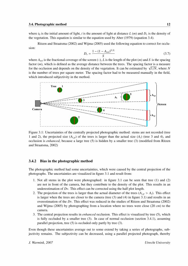
Ritzen and Straatsma (2002) and Wijma (2005) used the following equation to correct for occlu-sion:
Dv =1 − (1 − Atot)S/L
S(3.7)
where Atot is the fractional coverage of the screen (–), L is the length of the plot (m) and S is the spacingfactor (m), which is defined as the average distance between the trees. The spacing factor is a measurefor the occlusion and depends on the density of the vegetation. It can be estimated by
√1/N, where N
is the number of trees per square meter. The spacing factor had to be measured manually in the field,which introduced subjectivity in the method.
Figure 3.1: Uncertainties of the centrally projected photographic method: stems are not recorded (tree1 and 2), the projected size (Ai,p) of the trees is larger than the actual size (Ai) (tree 3 and 4), andocclusion is enhanced, because a large tree (5) is hidden by a smaller tree (3) (modified from Ritzenand Straatsma, 2002)
3.4.2 Bias in the photographic method
The photographic method had some uncertainties, which were caused by the central projection of thephotographs. The uncertainties are visualized in figure 3.1 and result from:
1. Not all stems in the plot were photographed: in figure 3.1 can be seen that tree (1) and (2)are not in front of the camera, but they contribute to the density of the plot. This results in anunderestimation of Dv. This effect can be corrected using the half plot length.
2. The projection of the trees is larger than the actual diameter of the trees (Ai,p > Ai). This effectis larger when the trees are closer to the camera (tree (3) and (4) in figure 3.1) and results in anoverestimation of the Dv. This effect was reduced in the studies of Ritzen and Straatsma (2002)and Wijma (2005) by photographing from a location where no trees were close (20 cm) to thecamera.
3. The central projection results in enhanced occlusion. This effect is visualized by tree (5), whichis fully occluded by a smaller tree (3). In case of normal occlusion (section 3.4.1), assumingparallel projection, tree (5) is occluded only partly by tree (3).
Even though these uncertainties average out to some extend by taking a series of photographs, sub-jectivity remains. The subjectivity can be decreased, using a parallel projected photograph, thereby
J. Warmink, 2007 Utrecht University

3.5. Terrestrial laser scanning 13
decreasing the uncertainties described above. A correction for “normal” occlusion, remains necessary.The method to measure vegetation density using parallel photography is described in chapter 5.
3.5 Terrestrial laser scanning
Terrestrial laser scanning (TLS) is increasingly being appreciated as an efficient tool for fast and reli-able 3D point cloud data acquisition. It has a wide range of application fields like, 3D visualizationof industrial structures, infrastructure and architecture (Lemmens and van den Heuvel, 2001, ; figure3.2). TLS measures distances using a laser range finder. Laser scanners generate a 3D point cloudrepresenting the surface of objects. The quality of the 3D point clouds generated by laser scanners andthe automation potential make TLS also an interesting tool for forest inventory (Bienert et al., 2006).
Figure 3.2: Examples of application of TLS in digitization of industrial structures (left) and infrastruc-ture (right) (from: www.delfttech.nl)
3.5.1 Technical specifications of terrestrial laser scanners
Laser scanners that are currently on the market can be categorized by different criteria:
• Field of View: laser scanners generally have a panoramic field of view of 360 ◦ horizontally anda one–side vertical field of view between 80◦ and 135◦ (Bienert et al., 2006).
• Range measurement principle: time of flight or phase–modulation based (Frohlich and Metten-leiter, 2004).
Today, the most popular measurement system is the time of flight principle, which allows up to severalhundred of meters. Laser scanners using the time of flight principle fire discrete laser pulses. Thedistance is calculated from the pulse travel time between emission and return of the pulse (Straatsmaand Middelkoop, 2006). Besides the time of flight principle, the phase based measurement principle isanother common technique. The phase–modulation laser scanners determine the distance to the targetfrom the phase difference of the return pulse of a continuously emitted laser signal (Straatsma andMiddelkoop, 2006). This type of scanner has smaller ranges, limited to 100 m, but a higher accuracylevel. The specifications of three different scanners are presented in table 3.2 (Frohlich and Mettenleiter,2004).
J. Warmink, 2007 Utrecht University

3.5. Terrestrial laser scanning 14
Other parameters are: (1) Scanning speed. In general the time of flight based scanners are slowcompared to phase based scanners. (2) Spatial resolution i.e. the number of points scanned in the fieldof view. The spatial resolution determines the point density. (3) Accuracy and range of the instrument.An instrument with a large range will generally have lower accuracy (table 3.3). (4) The combinationwith other devices mounted on the laser scanner. Some scanners are equipped with a built–in GPSinstrument or a digital camera, for the acquisition of high resolution surface texture and the fusion ofpoint cloud and image data processing (Bienert et al., 2006). Forest inventories need a high samplingrate of at least 10 kHz (Bienert et al., 2006) and a large field of view.
When multiple echoes return from a single pulse, ghost points are created. Ghost point are pointswhich have an erroneous distance, because the distance is calculated from the average of the traveltimes of the two returned pulses. As a consequence, the location of the ghost point in the point cloudis erroneous. Ghost points are produced when some twigs partly occlude each other and have to beconsidered in the development of data processing schemes (Bienert et al., 2006).
3.5.2 Application of terrestrial laser scanning in forestry
Previous research focussed on object extraction of individual trees using TLS, which could be convertedto vegetation density. The first step in this process is the generation of a Digital Terrain Model (DTM)from the laser scan data.
DTM generation
A simple approach to DTM generation was used by Aschoff et al. (2004). The authors laid a grid overthe scanned plot and selected the point with the lowest z value in each grid cell to be the ground point,excluding the points above a certain threshold. Subsequently, all points with similar z values, were clas-sified as a ground point or a vegetation point. Afterwards, a filter was applied to remove misclassifiedpoints from the ground point data set. The final steps in DEM generation were the visual removal ofmisclassified ground points and the creation of a continuous surface using interpolation (Aschoff et al.,2004). This simple approach gave satisfactory results in this study, but more sophisticated methodshave been employed Kraus and Rieger (1999).
Geometrical shape fitting
3D terrestrial laser scanning has been used to map forest stands and to digitize individual trees by geo-metrical shape fitting (Thies et al., 2004) (figure 3.3). For the digitization of trees the points classified
Table 3.2: Examples of the technical specifications of TLS systems (Frohlich and Mettenleiter, 2004).System Scanner type Meas.
principleFreq. Range Accuracy
Leica HDS3000 Panoramic Pulse 1 kHz > 100 m 6mm @ 50mOptech ILRIS–3D Camera (small hor.
field of view)Pulse 8 kHz 800 m 3mm < 100m and
1–3cm > 100mZoller & FrohlichIMAGER 5003
Panoramic Phase 500 kHz 52 m –
J. Warmink, 2007 Utrecht University

3.5. Terrestrial laser scanning 15
as vegetation are used for shape fitting. The primary interest in the shape fitting process lies in thediameter and the growing direction of the tree. Therefore, Thies et al. (2004) used an approach, wherea cylinder model was fitted to a segment of the point cloud. After successful fitting in one segment,the next cylinder was fitted to a new selection of points, to describe the stem in the next section. Thisresulted in an overlapping sequence of cylinders describing the radius and orientation of the stem as itchanges with height.
Bienert et al. (2006) proposed a technique for point cloud segmentation to detect diameters atbreast height and diameter–height profiles. Diameter–height profiles proved valuable to vegetationroughness calculation (Baptist, 2005). The diameter at breast height was determined by cutting a sliceat 1.3 meter above ground level. An adjusting circle was fitted into the 2D projection of the points ofthe slice. Proceeding with this technique stem diameters at every height can be determined.
(a) The reflection intensity decreases withdistance (Thies et al., 2004)
(b) Single tree scanned from 4 directionsfor detailed digitization (Gorte and Winter-halder, 2004)
(c) Diameter–heightprofile (Bienert et al.,2006)
Figure 3.3: Examples of terrestrial laser scanning applications on forest stands
Table 3.3: Classification of scanners on the range measurement principle (Frohlich and Mettenleiter,2004)
Range principle Range (m) Acc. (mm) ManufacturersTime of flight < 100 < 10 Callidus, Leica, Mensi, Optech, Riegle
< 1000 < 20 Optech, RieglePhase modulation < 100 < 10 IQSun, Leica, VisImage, Zoller & Frohlich
J. Warmink, 2007 Utrecht University

3.5. Terrestrial laser scanning 16
The voxel approach
Gorte and Winterhalder (2004) used a different approach, where they first converted the 3D point cloudinto the 3D grid domain. The cells in a 3D grid were small cubes called voxels (volume elements asopposed to pixels in 2D). The grid size of the cells determined the resolution of the 3D grid. During theconversion of a point cloud to a 3D grid, the xyz position of a point, together with the chosen resolution,determined the position of the corresponding voxel. The voxels were given the value of the number oflaser hits in a voxel. After the conversion to voxels, they used 3D raster processing techniques insteadof point calculations to create a voxel representation of a single tree, including topology, such as stem,branches and twigs.
Chasmer et al. (2004) applied the voxel technique on a larger scale, to compare the ALS and TLSmethods, for vegetation mapping purposes in a forested area. They concluded that the airborne methodwill likely underestimate the leafy biomass within the canopy, and may influence measures of LAI, dueto the hiding of lower leafs by the overlying canopy. The TLS method underestimates the tree heightdue to the same effect. The voxel approach made it possible to quantify the difference between theairborne and terrestrial methods in 3D space. The study illustrated that, due to occlusion, substantialparts of the understory and canopy are excluded from ALS and TLS respectively.
TLS methods for vegetation density mapping
From these studies, it can be concluded that the TLS method is promising for determining the vegetationdensity of forests. In combination with automatic data processing tools, the gap between conventionalinventory techniques and laser scanning may be bridged (Bienert et al., 2006). The advantage of theTLS method is that 3D images of vegetation density can be generated, which may be valuable forcomparison with ALS.
J. Warmink, 2007 Utrecht University

Chapter 4
Study areas
This study was carried out in two floodplains along the rivers Rhine and IJssel in The Netherlands: theGamerensche Waard (GW) and the Duursche Waarden & Fortmond (DW).
Figure 4.1: Location of the Gamerensche Waard (GW) and the Duursche Waarden (DW) floodplain
4.1 The Gamerensche Waard
The Gamerensche Waard floodplain is located at the left bank of the river Waal, the main branch of theRhine river distributaries (figure 4.1). The floodplain is located west of the city of Zaltbommel, in anouter bend of the river. The geomorphology consists of levee deposits and three artificial side channels.The floodplain area is flooded, annually, over a large area at high discharges. The area of the old brickfactory (appendix A.1) is the highest point of the floodplain and is rarely flooded (figure 4.3(b)). Thesize of the floodplain is about 73 hectares and it is developed as a nature area. In 1996, three side
17

4.2. The Duursche Waarden & Fortmond 18
channels were constructed, one perennial and two channels close to the main channel, ephemeral. Theruin of the brick factory was removed in the same period (figure 4.2).
Since 1996, an intensive vegetation monitoring program exists for the Gamerensche Waard.Throughout the year, the whole floodplain is grazed by horses, in the growing season also cows arepresent. The dominant vegetation consists of softwood willow forest (Salix alba, Salix viminalis) andgrassland with creeping thistle (Cirsium arvense) and stinging nettle (Urtica dioica) patches (Jesse,2004). Several ecotope maps were made of the area during the monitoring of the development of theside channels (Jans, 2004). Information on the temporary development of the vegetation classes is,therefore, available (Van Velzen et al., 2003b; Jesse, 2004). The area of natural grassland has decreasedsince 1996 and is replaced by dry herb vegetation or softwood forest.
Figure 4.2: Aerial photograph of the GW floodplain area, with the TLS forest upper left
Measurement locations in the GW
In the Gamerensche Waard, TLS was carried out in a willow forest patch. The forest was 80 meter wideand 120 meter long (figure 4.3(c) and 4.3(d)). The edges of the forest were dense and the central partshad a more open structure. The elevation differences inside the forest area were small, with a maximumof 0.5 meter. Little undergrowth was present, only some patches of stinging nettle. The horses and cows,which were present in the floodplain area, had removed most undergrowth (figure 4.5(c)). Besidesthe TLS measurements, 12 forest plots were measured in the forest using the photographic method.Additionally, 10 plots of dry herb vegetation and dense softwood forest were measured, elsewhere inthe floodplain area. The measurement locations are shown in appendix A.2.
4.2 The Duursche Waarden & Fortmond
The Duursche Waarden & Fortmond floodplain is located at the right bank of the river IJssel, a sidebranch of the river Rhine. It is located 10 km north of the city of Deventer (figure 4.1). The DuurscheWaarden area is a nature reserve, while the area around Fortmond is dominated by cultural land andforest (figure 4.4; appendix A.1). The geomorphology consists of a point bar with a side channel
J. Warmink, 2007 Utrecht University

4.2. The Duursche Waarden & Fortmond 19
(a) Summer impression of the GW (b) Winter impression of the GW
(c) The laser scan forest (d) The laser scan forest in winter conditions
Figure 4.3: The Gamerensche Waard under summer and winter conditions
connected at the downstream end, and a river dune. The dead arm and a sand pit were connected in1989 to the main channel. The area is grazed by horses and cows with 0.8 animals per hectare (Jesse,2004). This resulted in extensively grazed vegetation, consisting of natural grasslands with patches ofshrubs and herb vegetation and forest in various stages of development (e.g. softwood willow (Salixalba, Salix viminalis), poplar (Populus nigra, Polpulus x canadensis) and ash (Fraxinus excelsior)). Thetypical inundation depth of these floodplains is 3 m, but water depths may rise to 5 m in case of extremefloods.
The Fortmond area is characterized by several houses and farms, which are located along theroad (figure 4.4; appendix A.1). This area is used for agriculture and the vegetation is dominated byproduction grassland and agricultural crops. The area around the old brick factory is high and accessiblein winter and open for recreational use. A camping site is present along the IJssel, in the southern partof the floodplain. The forest near Fortmond is more than 40 years old and consists of oak (Quercusrobur), beech (Betula pendula) and a small mature pine stand (Pinus sylvestris). The centre part of theforest lies between 4 and 8 m above sea level and is rarely flooded. The western part of the forest islower and flooded regularly. The nature reserve area is flooded during a large part of the winter.
In 1989, the DW was the first floodplain that was subjected to landscaping measures by theMinistry of Transport, Public Works and Water management (Jesse, 2004). Ever since, this area is a
J. Warmink, 2007 Utrecht University

4.2. The Duursche Waarden & Fortmond 20
Figure 4.4: Aerial photograph of the DW floodplain area, with the Fortmond area in the western part ofthe floodplain and the nature reserve in the north (from: www.googleearth.com)
nature reserve, and the vegetation is intensively monitored. The vegetation is dominated by naturalgrassland, herb vegetation and softwood forest. The area covered with grasslands is reduced since1989, while the areas with dry herb vegetation, thorn shrubs and softwood forest have increased. Smallsoftwood forest stands were present between the fields. The high area around the old brick factoryconsists of herb vegetation, with isolated trees and shrubs. Several small fields of reed are present alongthe river. On the river dune, the only hardwood forest vegetation in the study areas is located. In thisthesis, the name Duursche Waarden (DW) will be used for the combined area of the nature reserve andthe area around Fortmond.
Measurement locations in the DW
In the DW floodplain, 51 vegetation plots were measured. The photographic method was used to de-termine the vegetation density in different vegetation types. The measurement locations are presentedin appendix A.2. Five herbaceous plots were measured again under winter conditions. In winter, how-ever, most areas of the floodplain were flooded (figure 4.5(d)), due to a high river discharge. Therefore,not all vegetation types could be duplex measured under winter conditions. The locations, measuredin summer in the nature reserve area were flooded (figure 4.5(b)). So the duplex measurements werecarried out near the old brick factory, which was the only location with herbaceous vegetation, whichwas not flooded. The locations of the duplex measured plots are shown in appendix A.2.
J. Warmink, 2007 Utrecht University

4.3. Plot selection 21
(a) Measurement area in summer conditions (b) The same area during flooding
(c) Little undergrowth in the TLS forest in the Gameren-sche Waard
(d) Flooding of the Duursche Waarden
Figure 4.5: Flooding of the measurement area (a,b) and impression of the study areas (c,d).
4.3 Plot selection
In the floodplain areas of the Duursche– and Gamerensche Waard the measurement plots were selected,initially, based on the DTB-river maps that show topographical descriptions of the vegetation (appendixA.2). During the measurements, the vegetation type of the measured plot was recorded. The vegetationtypes are based on the vegetation mapping studies by Van Velzen et al. (2003a) and Jesse (2004). In eachvegetation type with natural vegetation, if possible, at least 5 plot locations were measured. Agriculturalvegetation types were not measured, due to time limit actions. The measured vegetation types are:
a hardwood forest with oak (Quercus robur) and ash (Fraxinus excelsior),b softwood willow forest (Salix alba, Salix viminalis),c shrub vegetation consisting of hawthorn (Crataegus laevigata),d natural grassland consisting mainly of grass (Lolium perenne) and clover (Trifolium repens),e herbaceous vegetation with dominant creeping thistle (Cirsium arvense), grass, stinging nettle and
dewberry (Rubus caesius),f herbaceous vegetation with dominant stinging nettle (Urtica dioica), dewberry, creeping thistle and
grass,g herbaceous vegetation, with high species diversity, consisting of stinging nettle , grass, great bind
J. Warmink, 2007 Utrecht University

4.3. Plot selection 22
weed (Calystegia sepium), dewberry and the great willow herb (Epilobium hirsutum) andh reed marshes (Phragmites australis).
Representative plots were selected for each class. The fractions of high and low vegetation inthe area were reflected in the measurement plot. This fractions was estimated visually in the field. Theplot size of the herbaceous plots was about 2 m wide and 0.5 m long and forest plots were 5 meterwide and between 5 and 10 meter long. The forest plots were delimited in a rectangle, and no treeswere intersecting the edges of the plot. A single plot of hawthorn brushwood was measured. Themeasurement locations including the mapped vegetation types are presented in appendix A.2
J. Warmink, 2007 Utrecht University

Chapter 5
Vegetation density measurements methodusing parallel photography
The centrally projected, photographic method has several limitations. Therefore, I propose a newmethod to measure vegetation density in the field: the parallel photographic method (PP). A paral-lel image mosaic was created, by merging multiple photographs, taken along a parallel transect. Themethod was validated on simple vegetation structures and applied to more complex vegetation types.
5.1 Reference data collection
In the Gamerensche Waard and Duursche Waarden floodplain sections, 68 measurements were carriedout using the PP method. The vegetation type and the parameters, like the camera setting and the plotsetup. which influenced the PP, were recorded on the field form (appendix C.1). The coordinates of theplot centre were measured using GPS with an accuracy of 5 meter. Furthermore, the weather at the timeof the measurement was recorded. The ground height at the location of the plot was estimated based ona height map.
5.1.1 Manual vegetation density measurements
The reference data for forest plots was collected by measuring the circumference of all trees in a plot atbreast height, which was defined as 1.3 m above the ground surface. The diameter was calculated fromthe circumference by division through π. Multiplying the average diameter of all trees in the plot bythe number of trees per square meter, yielded an estimation for the vegetation density (DvNd; equation2.4).
The reference data of the herbaceous plots was measured similarly, with the exception that notall stems in each plot were measured, but 30 stems were randomly selected at the half vegetation height(the height where the photographs were taken). The diameter was measured using a sliding gauge,with an accuracy of 0.1 mm. When the stems were not cylindrical, the average diameter was estimated.Subsequently the total number of stems was counted in the plot and divided by the measured surfacearea of the plot. For the first 14 herb plots the DvNd value was measured at 15 cm above ground levelinstead of at the photo height, leading to an overestimation of Dv.
This measurement method was based on the assumption that all vegetation elements were cylin-
23

5.2. The parallel photographic method 24
drical. These assumptions are valid when all stems are straight and vertically orientated and have noside branches or leaves. The plots, which satisfied these conditions were used to validate the PP method.The validation plots were selected in the field by recording the number of side branches. Seventeen for-est plots, with less than 10 small side branches were used for the validation of the parallel photographicmethod.
5.1.2 Vegetation height measurements
Additionally, the vegetation height of all herb plots was determined by measuring the length of the same30 stems used for the density calculation. The length of these 30 stems was measured from the top tothe ground surface using a folding rule. Furthermore the length of the highest stem in the plot (Hvmax)and the highest representative stem (Hvrep) are recorded. The highest representative height is definedas the highest leaf or when leaves are absent the height of the layer of highest stem (figure 5.1).
The selection of 30 stems at the photo height resulted in an overestimation of the average vegeta-tion height, because vegetation lower than the photo height was not included in the height determination.For some plots a separate height measurement was taken, where the stems were randomly selected at15 cm above the ground surface, instead of the photo height. The 30 stems were selected just abovethe ground surface. This gives a better representation of the average vegetation height. The vegetationheight measurement data is needed for the calculation of vegetation roughness in future studies. It is,however not part of this research. The results are presented in appendix C.2.
Figure 5.1: Definition of maximum vegetation height (Hvmax), representative maximum vegetationheight (Hvrep) and the average vegetation height (Hvaverge)
.
5.2 The parallel photographic method
The PP consists of taking multiple photographs of the vegetation against a contrasting background alonga line, parallel to the screen. From these photographs, the centre columns were clipped and merged toproduce a single parallel projected photo mosaic for each measurement plot.
J. Warmink, 2007 Utrecht University

5.2. The parallel photographic method 25
Figure 5.2: Approach to the parallel photographic methods: (a,b) setup of the guide rail for the cam-era and background for forest and herbaceous vegetation, (c,d) derived parallel photo mosaics, (e)histogram of intensity values (0 to 255) with threshold, (f) histogram of hue values (0 to 360) withthresholds, (g,h) thresholded images (from Straatsma et al., submitted)
5.2.1 Field setup to the parallel photographic method
The PP method required a contrasting background screen, digital camera, measuring tape, a 6 m longguide rail (divided in two parts of 3 m), 3 tripods to support the rail, an 80 cm and a 5 cm long level, asurveyors beacon, clips to fixate the rail to the tripod and a laptop. The plot was selected as describedin section 4.3. In herbaceous vegetation a plot was prepared in a vegetation stand by selecting a 2 mwide and about 50 cm long area. A red screen of 2 m high and 2.5 m wide was placed behind thevegetation, with a backward angle to reduce shadows. The plot was created by removing or flatteningthe vegetation in front of the plot. The length of the plot was determined, so the screen was coveredfor 50 % (figure 5.2). The guide rail was set up parallel to the screen. The guide rail of 3 m was usedin herbaceous plot and the 6 m long rail, in forest plots. The rail was levelled, in front view, using thelong level, by adjusting the height of the tripods, and in side view by changing the forward angle on thetripods. The camera was fixed on the rail, so only sideward movement was possible. The digital camerawas moved along a guide rail and at small intervals (1 cm in forest plots and 5 cm in herbaceous plots)a photograph was taken. In this research a Canon PowerShot 520A was used, where the exposure couldbe set manually. The photographs of the forest plots were slightly underexposed, because the shuttertime had to be larger than 1
15 to ensure sharp images. The herb plots were set at a good exposure. Theaperture was set as large as possible, to maximize the depth of view.
The shutter time and aperture were set manually, so all photographs had equal exposure. Threecalibration photographs were made of the surveyors beacon: left, right and in the centre of the plot,
J. Warmink, 2007 Utrecht University

5.2. The parallel photographic method 26
to calculate the number of pixels represented by the sliding distance. The parallel photographs weretaken by sliding the camera over the rail from left to right, with fixed intervals: every 5 cm for forestplots and 1 cm for herbaceous plots. The forward tilt was checked at each photograph using the smalllevel and corrected if necessary. Most plots were measured with the camera at a small opening angle(±12◦ i.e. fully zoomed in). The resolution was set at 2272x1704 pixels. To study the effect of theresolution, some plots were also measured with a larger opening angle (±46◦ i.e. zoomed out), anddifferent resolutions were applied. For every forest plots about 100 pictures were taken, for herbaceousplots about 200. The photographs were transferred to the laptop, after each plot, to avoid remountingthe camera during the measurement.
For comparison, the centrally projected method (Ritzen and Straatsma, 2002), was also appliedto plots (section 3.4). The same field setup, without the guide rail was used and 8 photographs weretaken at the same distance and height as the PP method. The zoom was fixed and the whole plot wasvisible at each photograph.
5.2.2 Creation of a parallel photo mosaic
The centre columns of the plot photographs were merged, to create a parallel projected photo mosaicof the plot. This was done by calculating the number of columns (w) in pixels representing the slidinginterval over the guide rail (figure 5.3). The equation used to calculate the width value is:
w = ppm · d (5.1)
where ppm =xres
2Dp · tan 12α
(5.2)
and α = 2 arctan12 ccd
f(5.3)
where ppm is the number of pixels per meter (pix · m−1), d is the horizontal sliding distance (m), xres
is the resolution along the x–axis of the photograph (2272), Dp is the distance from the camera to thescreen (m), α is the opening angle, which depended on the zoom, ccd is the horizontal size of the sensorrecording the picture (5.69 mm) and f is the focal length of the lens (23.2 mm, with zoom and 5.8 mmwithout zoom). These values were derived from the manual of the camera.
This calculation assumes that a pixel in the centre of the picture represents an equally largesurface area as a pixel at the side of the photograph. Because only the centre columns of the photographswere taken, overestimation of the surface area is avoided. Furthermore, the number of centre columnsdepend on the zoom, resolution and sliding interval. The only parameter measured in the field inthis calculation is the distance from the camera to the screen. The calculated number of columnswere consistent with the measured number of columns using the surveyors beacon. For zoomed inphotographs, with a horizontal resolution of 2272 pixels, the number of pixels per meter ranged between550 and 9850 pix · m−1. The resolution for the photographs with a large opening angle was lower,between 365 and 1400 pix · m−1, depending on the plot length.
The calculated number of columns were clipped out of the original pictures and merged together.This was done using a script, written in the Python programming language. The flowchart and the scriptare presented in appendix B.1.
J. Warmink, 2007 Utrecht University

5.3. Data analysis 27
Figure 5.3: Calculation of the width of the clipped centre columns.
5.3 Data analysis
The vegetation density (DvPP) was calculated from the parallel photo mosaic by:
DvPP = − 1L· ln (1 − Atot) (5.4)
where Atot is the fractional coverage of the screen by vegetation and L is the plot length. This equationis similar to the description of vegetation density by MacArthur and MacArthur (1961) and Aber (1979)(equation 3.3 and 3.4). The term 1
L was included to make DvPP independent of the plot length.
5.3.1 Intensity thresholding
To determine the fractional coverage of the screen by the vegetation a threshold operation was applied,based on the intensity histogram of the mosaic. The mosaic was converted from full color to a binaryimage, where vegetation pixels were set to black, and screen pixels were set to white. The thresholdwas set manually, based on the intensity histogram. Shadows on the screen and the effect of mixedpixels (partly screen and partly vegetation) caused overlap in intensity values between the two classes.The percentage of black pixels was calculated and yielded the fractional coverage. A GNU ImageManipulation Program The Gimp 2.2 (2006) (www.gimp.org) was used to perform the thresholding.The beginning of the second peak in the intensity histogram proved a visually correct threshold value(figure 5.4(a)).
5.3.2 Hue thresholding
For herb vegetation a red screen was used as background, to increase the contrast between screen andvegetation. However, the discrimination between screen and vegetation by intensity thresholding re-sulted in high uncertainties, because the red screen and green vegetation had similar intensities. There-fore, the RGB (Red, Green, Blue) picture was converted to HSV (Hue, Saturation, Value). The huevalue represents the color type as a value between 0 and 360 degrees (figure 5.5), where red has a valueof zero. Subsequently, the threshold was applied on the hue value. Shadow and light intensity havelittle influence on the discrimination (Lillesand et al., 2004). Besides that the hue value was a betterdiscriminator for herb vegetation, another advantage was that the threshold value was equal for eachplot because the screen had a fixed color. The threshold values were determined for a single plot and
J. Warmink, 2007 Utrecht University

5.3. Data analysis 28
(a) (b)
Figure 5.4: A histogram of the intensity of the mosaic of a forest plot and a hue histogram of the mosaicof a herbaceous plot. The threshold value was based on these histograms
subsequently applied to all other plots. The histogram of the hue is presented in figure 5.4(b) and thethreshold values are drawn in figure 5.5. The histogram and the HSV circle show that the screen area isset from 300◦ to 15◦, where 15◦ is the border between red and orange.
Figure 5.5: Hue, saturation, value circle, where the hue (H) is presented as the circle from 0 to 360degrees, the saturation (S) ranges from full color to gray and the value or intensity (V) ranges fromblack to white
The medical image processing and visualization program MeVisLab (2006) was used to convertthe RGB images to HSV and calculate the fractional coverage. A trial version can be downloaded fromwww.mevislab.de. This program has build–in modules for HSV conversion, thresholding and coveragecalculation. In MeVisLab, the procedure can be automated. DvPP was computed using Excel, with the
J. Warmink, 2007 Utrecht University

5.3. Data analysis 29
coverage values from MeVisLab as described above. The flowchart of the procedure is presented inappendix B.1. Figure 5.2 shows the approach used for the PP method in an overview.
5.3.3 Comparison to the reference data
The vegetation densities, measured by the reference data (DvNd) were compared to DvPP using scatterplots. In this study, regression analysis was used between the measurement methods. R2 is a measurefor the amount of explained variance, and expresses the strength of the relation acquired by regressionanalysis. Subsequently, a student’s t–test was applied to test if the slope of the regression line wassignificantly different from 1. To test if the within–subject variation depended on the vegetation density,the residuals (i.e. reference minus predictor) were plotted against the reference. Furthermore, thestandard error (SE) of the residuals was calculated.
J. Warmink, 2007 Utrecht University

Chapter 6
Results of the photographic methods
In this chapter, the results from the field measurements using the parallel and centrally projected (CP)photographic methods are presented. At first instance, the methods were validated, subsequently, thePP method was applied to plots with different vegetation types, in summer and winter.
6.1 Validation of the photographic methods
6.1.1 Central projected method
Figure 6.1(a) shows the scatter plot of the selected validation plots, measured by the CP method. Thereference values were plotted on the vertical axis and the DvCP on the horizontal axis. Only 11 outof the 17 validation plots, were measured by the CP method. The y = x line is shown in red, in thefigure. The Dv ranges from 0.014 m−1 for open forest to 0.12 m−1 for dense parts of the forest and theDvCP increases linearly with the reference data. This figure shows that linear regression explained areasonably large part of the variance (R2 = 0.87). The regression equation and the standard error of thesigned residuals to the y = x line are presented in table 6.1.2.
The signed residuals of DvCP to the line of identity are plotted in figure 6.1(b). The negativeresiduals in the scatter plot of the residuals show that the DvCP was overestimated. The overestimationcan be explained by the increased projection of the trees on the screen (figure 3.1). No relation waspresent between the errors of the DvCP and the vegetation density. The DvCP shows a reasonablylarge scatter, with a maximal deviation of 0.025 m−1. Few measurements of dense forest, with DvNdvalues above 0.07 m−1 are present. This can be explained by a, generally, increasing complexity withincreasing density. Therefore, these plots could not be used for validation purposes.
6.1.2 Parallel projected method
The scatter plot of the validation of the PP method is presented in figure 6.2(a). The range of the DvPP
values was similar to the DvCP, and the DvPP increased linearly with the manually measured data. ThePP method proved well able to predict vegetation density of floodplain forest: the linear regressionmodel with a zero intercept, explains 99.6 percent of the variance. The regression function is given by:
DvNd = 1.0059 · DvPP (n = 17,R2 = 0.996, S E = 3.7 · 10−3) (6.1)
30

6.1. Validation of the photographic methods 31
0.00
0.04
0.08
0.12
0.00 0.04 0.08 0.12
Dv N
d (
m-1
)
DvCP (m-1)
R2 = 0.87
(a) Performance of the CP method in the valida-tion plots
-0.03
-0.02
-0.01
0.00
0.01
0.00 0.04 0.08 0.12
Re
sid
ua
ls
DvN d (m-1)
(b) Signed residuals of the CP method to the y = xline
Figure 6.1: Scatter plots of the validation of the centrally projected photographic method
Figure 6.2(b) shows the residuals of the DvPP. The maximal absolute error was 0.008 m−1, which wassmaller than for the DvCP. The residual standard error decreased from 0.010 for the CP method to0.0037 for the PP method. The residuals of the DvPP are scattered around the y = 0 line, indicating thatboth methods are highly comparable. A Students t–test, on the regression line, proved that the slope ofthe regression model did not significantly differ from 1, at the 99.9 percent confidence interval.
To test the performance of the PP method, for 5 plots, the manually measured diameters at breastheight of all the trees in a plot were compared to the diameters reconstructed from the parallel pro-jected photo mosaic. This comparison was done for the validation plots where no occlusion occurred.Reconstructing the diameters of a measured tree was done by making a map of the plot in the field,numbering all individual trees and measuring their diameters. The numbered trees on the map wererecognized on the photo mosaic, and the diameter, in pixels, was measured in an image manipulationprogram. Subsequently, the measured diameters were also converted to pixels using the width value(section 5.2.2).
The manually measured diameters were compared to the reconstructed values (figure 6.2(c)). Itshows that the projected tree size agrees with the measured diameter of the trees. The linear regres-sion model explained 97 percent of the variance. The figure of the signed residuals of the calculateddiameters (figure 6.2(d)) shows a decreasing error with an increasing size of the trees in pixels. Thisis caused by uncertainties in the diameter reconstruction, due to mixed pixels and errors in the numberof clipped centre columns. Mixed pixels occurred at the edges of the trees. When a mixed pixel wasdominated by screen, the reconstructed diameter was smaller than the measured diameter. Similarly,when a mixed pixel was dominated by vegetation the diameter was overestimated. The effect of theerror in the number of clipped centre columns was caused by rounding of the number of centre columnsto a whole number. This also caused over– or underestimation. Both effects caused random errors inthe reconstructed diameters. The errors were larger for smaller trees. These effects had a limited effecton the measurement method. The sensitivity of the clipped number of centre columns will be discussedfurther in chapter 7.
J. Warmink, 2007 Utrecht University

6.1. Validation of the photographic methods 32
0.00
0.04
0.08
0.12
0.00 0.04 0.08 0.12
Dv N
d (
m-1
)
DvPP (m-1)
R2 = 0.996
(a) Performance of the PP method in the valida-tion plots
-0.010
-0.005
0.000
0.005
0.010
0.00 0.04 0.08 0.12
Re
sid
ua
ls
DvN d (m-1)
(b) Signed residuals of the PP method to the y = xline
0
10
20
30
0 10 20 30
Me
as.
dia
me
ters
(p
ix)
Calculated diameters (pix)
R2 = 0.97
(c) Measured diameters versus the calculated di-ameters, based on the parallel projected photo mo-saics in numbers of pixels
-4.0
-2.0
0.0
2.0
4.0
0 10 20 30
Re
sid
ua
ls
Measured diameters (pix)
(d) Residuals of the measured and calculated di-ameters
Figure 6.2: Scatter plots of the validation of the PP method and the measured and calculated diameters
Table 6.1: Statistical expressions for the validation of the photographic methods, with the regressionequations, explained variance (R2) and residual standard error (SE)
Regression equation R2 S E sample size (n)CP method DvNd = 0.89 · DvCP 0.871 1.0 · 10−2 11CP residuals ErrCP = 0.15 · DvNd − 0.014 0.21 9.1 · 10−3 11PP method DvNd = 1.0059 · DvPP 0.996 3.8 · 10−3 17PP residuals ErrPP = 0.04 · DvNd − 0.002 0.08 3.7 · 10−3 17diameters dmeasured = 0.998 · dcalculated 0.97 1.1 37
6.1.3 Conclusions of the validation
It was proved that the PP predicted the vegetation density of the validation plots very well up to veg-etation densities of 0.12 m−1. The PP method was an improvement over the centrally projected pho-tographic method. For forest plots without side branches, the PP method performs equally well as themanual method for cylindrical vegetation. The PP method, however, is independent of the assumptionsunderlying the manual method (section 2.4). Therefore, the PP method will be used as a measurement
J. Warmink, 2007 Utrecht University

6.2. Application of the parallel photographic method on complex vegetation 33
tool to estimate the vegetation density of more complex vegetation structures. The regression equa-tions, explained variance and residual standard errors for the validation of the photographic methodsare presented in table 6.1.2.
6.2 Application of the parallel photographic method on complex vegeta-tion
To test the applicability of the PP method on more complex vegetation structures, the method wasused to measure a wide range of vegetation types in the Gamerensche Waard and Duursche Waardenfloodplains. Because the PP is a better estimator for the vegetation density of complex vegetation thanthe manual method, the DvPP was considered as reference data. The results are presented in figure6.3, where the DvNd is plotted on the horizontal axis and the DvPP on the vertical axis. The regressionequations and statistical coefficients are presented in table 6.2.2.
6.2.1 Variations in vegetation types and measurement technique
The results of the application of the PP method were categorized based on vegetation type and variationsin the measurement method. The selected categories were: (1) forest and shrub plots with more than 10side branches and leaves, (2) plots with herbaceous vegetation, measured with a small opening angle,(3) plots with herbaceous vegetation, where reference data was measured at 15 cm above ground leveland (4) plots with herbaceous vegetation, measured with a large opening angle. Figure 6.3 shows theparallel photo mosaics and thresholded images of these measurements.
Leaved forest plots
The scatter plot of the forest plots, which were not appropriate for validation, because many sidebranches or leaves were present, are shown in figure 6.4(a). These plots were measured using thewhite screen as background and the photographs were taken at breast height. The range of DvPP valueswas large, for these plots, compared to the validation plots, with DvPP values up to 0.23 m−1. The DvNdvalues, however, had the same range as the validation plots. The R2 value decreased from 0.996, forthe leafless validation plots to 0.62 for leaved forest plots. The residual standard error increased from3.7 · 10−3 to 3.8 · 10−2, accordingly.
The DvNd of leaved forest plots shows an underestimation, compared to the DvPP and a largescatter is visible in the figure. The underestimation was confirmed by the slope of the regression line ofthe residuals (figure 6.4(d)), which was significantly different from zero at the 99.8 confidence interval.The scatter plot of the residuals showed an increasing underestimation of the density as measured usingthe DvNd. This was caused by the increasing presence of side branches and leaves with stem density.The side branches and leaves were not measured by the manual method, but were included in the DvPP
measurement.
Herbaceous vegetation plots
The second category of measurements consisted of the herbaceous plots, where the manual method wasapplied at the photo height (figure 5.2). Figure 6.4(c) shows the scatter plot of the resulting DvPP values.
J. Warmink, 2007 Utrecht University

6.2. Application of the parallel photographic method on complex vegetation 34
(a) Validation forest plot (b) Thresholded image
(c) Leaved forest (d) Thresholded image
(e) Herbaceous vegetation (f) Thresholded image
(g) Measurements with a large opening angle (h) Thresholded image
Figure 6.3: Categories of the applications of the PP method for different vegetation types and variationsin the measurement technique. The parallel photo mosaics are shown at the right side, the thresholdedimages, on the left side. For the herbaceous vegetation, the pixels classified as background are shownin blue, for forest vegetation in white. From top to bottom: (a) forest plots used for validation, (c)forest plot with leaves, (e) herbaceous vegetation, measured with a small opening and (g) herbaceousvegetation, measured with a large opening angle.
J. Warmink, 2007 Utrecht University

6.2. Application of the parallel photographic method on complex vegetation 35
The DvPP of the herb plots was more than 15 times larger than for forest validation plots, ranging from0.7 m−1 to 2.0 m−1. A considerable fraction of the coverage consisted of leaves (figure 6.3).
The comparison of the DvPP and the DvNd (figure 6.4(c)), showed a bad correspondence with they = x line. When the residuals were taken into account, an average underestimation of 0.78 was visible.This underestimation was independent of the value of the DvPP. The residual standard error was quitelarge (0.14) for a sample size of 9 measurements. The underestimation was caused by the abundance ofleaves and side branches in the plots.
Lower layer of the herbaceous plots
Initially the DvNd method was measured at 15 cm above ground level, instead of at the photo height.To compare the photographic results with the DvNd, this layer was selected out of the parallel projectedphoto mosaic. The surveyor’s beacon, which is present on each photograph, was used to select layer atthe correct height. The selected layer had a height of 20 cm from 5 to 25 cm above ground level.
These lower layers showed very large DvPP values up to 6.2 m−1. The coverages of the screen byvegetation were close to 100 percent. The scatter plot (figure 6.4(e)) shows a large deviation of the lineof identity and a trend of increasing underestimation with increasing density. The regression line has aslope of 4.3, which means that the DvNd is at least 4 times larger than the DvPP.
Plots measured with a large opening angle
The last variation in the measurement method contained the plots which were measured with the cameraset at a large opening angle. This resulted in mosaics covering the vegetation from the ground surfaceto the top of the vegetation. Figure 6.3(g) shows that the range of the DvPP values between the top ofthe vegetation and the lower layer is large. The DvPP values calculated from these mosaics are averagedover the vegetation height. The averaged DvPP values are compared to the DvNd, measured at the halfvegetation height. The DvPP values are presented in figure 6.4(f). As expected, this resulted in a badcorrespondence to the y = x line and only 13 percent of the variance was explained by the regressionline. The figure shows that the DvNd underestimated the vertically averaged DvPP of the herbaceousplots.
6.2.2 Vegetation measured under winter conditions
To test the application of the PP method under winter conditions 5 plots were duplex measured. Thissmall sample resulted from the flooding of the floodplains at high discharges, which occur frequentlyin winter and limited the area for research. During this fieldwork in the winter 90 % of the herb plotsmeasured in the summer were flooded. Furthermore, parts of the floodplains were mowed, therefore,most plot measured in summer could not be measured again in winter. The 5 remaining plots werevegetation test areas in the DW, used for a different research, and were therefore not mowed. Theduplex measured plots belong to the species rich herbaceous vegetation type. Under winter conditionsthe dewberry (Rubus caesius), was the dominant species in the plot.
The scatter plot of the winter measurements is presented in figure 6.5(a). It can be seen thatthe range of DvPP values was smaller under winter conditions, with a maximum of 0.91 m−1, than insummer, when the maximum DvPP value was 2.9 m−1 for the same plot. The explanation of the varianceby the regression equation is 0.88, but it must be noted that this value is biased, because the sample size
J. Warmink, 2007 Utrecht University

6.2. Application of the parallel photographic method on complex vegetation 36
0.00
0.10
0.20
0.00 0.10 0.20
Dv
PP (
m-1
)
DvN d (m-1)
R2 = 0.64
(a) DvPP of the leaved forest plots
-0.04
0.00
0.04
0.08
0.12
0.00 0.10 0.20
Re
sid
ua
ls
DvPP (m-1)
R2 = 0.63
(b) residuals of the leaved forest plots
0.0
1.0
2.0
0.0 1.0 2.0
Dv
PP (
m-1
)
DvN d (m-1)
R2 = 0.83
(c) DvPP of the herbaceous plots
0.50
0.75
1.00
0.50 1.00 1.50 2.00
Re
sid
ua
ls
DvPP (m-1)
R2 = 0.023
(d) residuals of the herbaceous plots
0.0
2.0
4.0
6.0
0.0 2.0 4.0 6.0
Dv
PP (
m-1
)
DvN d (m-1)
R2 = 0.77
(e) The DvPP of the lower layer (15 cm aboveground level)
0.0
1.0
2.0
3.0
0.0 1.0 2.0 3.0
Dv
PP (
m-1
)
DvN d (m-1)
R2 = 0.13
(f) The DvPP, vertically averaged over the vegeta-tion height
Figure 6.4: Scatter plots of the application of PP on (a) leaved forest plots, (c) plots consisting of herba-ceous vegetation, measured at the half vegetation height with a small opening angle, (e) herbaceousplots measured at 15 cm above ground level, with a small opening angle, and (f) herbaceous plots mea-sured at the half vegetation height, with a large opening angle, resulting in vertically averaged DvPP
values
J. Warmink, 2007 Utrecht University

6.2. Application of the parallel photographic method on complex vegetation 37
is small. The point with the highest DvPP value shows an underestimation, while the other points arelocated closer to the line of identity. A possible explanation is that, generally, at higher vegetationdensities, more side branches are present and, therefore, the underestimation of the DvNd increaseswith increasing vegetation density. Only a single measurement of relative dense vegetation was doneunder winter conditions, so no trend can be seen.
The comparison between the DvPP measured under summer and winter conditions is presentedin figure 6.5(b). It can be seen that the summer measurements show a large overestimation. Regressionanalysis showed no significant relation with the y = x line, between summer and winter measurements(p = 0.13), but no conclusions can be deducted, from these measurements, because of the low samplesize.
0.00
0.50
1.00
0.00 0.50 1.00
Dv
PP
,win
ter (m
-1)
DvN d (m-1)
(a) Vegetation measurements in winter
0.00
1.00
2.00
3.00
0.00 1.00 2.00 3.00
Dv
PP
,win
ter (m
-1)
DvPP,summer (m-1)
(b) Winter against summer vegetation
Figure 6.5: Scatter plots of the application of the parallel photographic method on complex vegetationstructures
Table 6.2: Statistical expressions for the application of the PP, with regression equations, explainedvariance (R2) and the residual standard error (S E). The expression with a “?” were unreliable, becauseof the small sample size. They were strongly influenced by a single measurement (figure 6.5)
Regression equation R2 S E nLeaved forest DvPP,leaved = 1.27 · DvNd + 0.020 0.64 2.4 · 10−2 12Leaved forest residuals Residual = 0.50 · DvPP,leaved − 0.017 0.63 3.8 · 10−2 12Herbs DvPP,herbs = 0.89 · DvNd + 0.81 0.83 0.15 9Herbs residuals Residual = 0.064 · DvPP,herbs + 0.68 0.02 0.14 9Lower layer DvPP,lower = 4.3 · DvNd + 0.23 0.77 0.19 15Vertically averaged DvPP,vertical = 1.5 · DvNd + 0.54 0.13 0.22 11Winter conditions DvNd = 0.60 · DvPP,winter + 0.081 0.98? 3.7 · 10−2 ? 5Summer – winter DvPP,winter = 0.46 · DvPP,summer − 0.53 0.88? 0.16? 5
J. Warmink, 2007 Utrecht University

6.2. Application of the parallel photographic method on complex vegetation 38
6.2.3 Time requirements
To asses the applicability of the PP in the field, the time required in the field is an important factor.Therefore, the time needed to measure a single plot was recorded (table 6.3). In the field, a screen andguide rail were placed in the vegetation, the photo camera was mounted on the rail and levelled andbetween 100 and 200 photographs were taken. For one person, it took about 20 minutes to measurea single plot, depending on the number of photographs and the processing speed of the camera andlaptop. The conversion from the individual photographs to a parallel photograph took approximately2 minutes using Python. Setting a threshold and calculating the vegetation density, took another 2minutes for each parallel photograph. In future studies the data analysis can be fully automated, exceptthe thresholding of the intensity value.
Table 6.3: Field time required for the PP methodAction Time (minutes) Depends onSetup screen 5 weatherSetup frame 5 experienceMaking photographs 5 – 15 number of photographsTransfer photographs to laptop 5 processing speedData analysis 4 level of automationTotal 29
J. Warmink, 2007 Utrecht University
Chapter 7
Accuracy and objectivity of the parallelphotographic method
The results indicate that the parallel photographic method is an improvement over the central photo-graphic method and the manual method. The DvPP values matched the DvNd values for the validationplots and showed consistent results on vegetation with a more complex structure. There are, however,several factors, which influence the prediction of the DvPP and determine the quality of the method.These will be discussed in this chapter.
7.1 Notes on the field technique
7.1.1 Quality of the reference data
The reference data for the validation of the PP method was collected using the manual method. Thediameter was measured using a sliding gauge for thin stems. For thicker stems the circumference wasmeasured using a measuring tape and the diameter was computed. These measurement instruments hada high accuracy. The assumption underlying the reference data was that the measured stems were cylin-drical. Because the assumption of cylindrical stems was never strictly true, the decision of the heightwhere the diameters were measured influenced the DvNd. The measurement height had a variation of10 cm, because the breast height was estimated visually and small difference in ground elevation werepresent. The error in the height of the diameter measurement was random and averaged out over theplot. This can result in an uncertainty in the vegetation density of about 5 percent, when few trees arepresent in the plot.
For herb plots, the average diameter was measured from 30 randomly selected stems. The sur-veyor was always inclined to take the conspicuous stems and forget the very small grass blades. Thisbehavior depends on the characteristics of the plot and caused large uncertainties in the DvNd. Becausethe results for a single plot are different for every surveyor, the effect is averaged out when more ob-servers are conducting the measurements. In this research, 95 % of the measurements were carried outby the same observer. The method, therefore, had a high degree of subjectivity and a low accuracy. Thesecond error in the DvNd measurement is caused by errors in the counted number of stems. Errors inthe number of stems may cause substantial errors in the DvNd. To minimize the error of the number ofstems, all stems above the photo height in the photographed area were counted. This area can be larger
39

7.1. Notes on the field technique 40
than ± 1 m2, containing several hundreds of stems. Therefore, errors in the counted number of stemseasily occur. Finally, the error in the measured surface area introduced an error in the average stemdensity.
The mapping of the vegetation type for each plot was done visually, using the vegetation manual(Van Velzen et al., 2003a). The vegetation types, sort rich herb vegetation, creeping thistle, stingingnettle and natural grasslands are overlapping and the decision when a plant type was dominant wasarbitrary and made this mapping subjective. The recorded vegetation types per plot are presented inappendix C.2.
7.1.2 Measurement time in the field
The time required in the field to measure a plot using the PP method was about 25 minutes, whichis long compared to the time needed for the CP method, which can be carried out between 5 and 15minutes (Ritzen and Straatsma, 2002). The time needed for the data analysis in this research (4 minutes),however, was less than the time indication mentioned by Ritzen and Straatsma (2002) (±15 minutes,based on 8 photographs per plot), due to a high level of automation. The time needed to measure thevegetation density using the manual method depended on the complexity of the vegetation. Measuringthe diameters of 30 stems using a sliding gauge took 5 minutes. Subsequently, the number of stemsin the plot must be determined. For simple vegetation (< 30 stems) the value was known from thediameter measurement, but for grass vegetation this took up to 30 minutes.
Table 7.1: Time needed to measure the Dv using the PP method compared to the CP method and themanual method
Action PP time CP time Nd timeSetup screen 5 min 5 – 20 min –Setup frame 5 min – measuring d of 30 stems:
5 minMaking photographs 5 – 15 min ±1 min counting all stems in plot:
1 – 30 minTransfer photographs to laptop 5 min 200 per 5 min –Data analysis 4 15 calc average diameter:
5 –15 minTotal 29 min 29 min between 10 and 60 min
7.1.3 Field equipment
The amount of material needed in the field for the PP method was large compared to the CP andthe manual method. At least two persons were needed to carry all equipment. The time needed forrelocation between plot locations can, therefore, be significant. For that reason, a hand chart was usedfor transporting the equipment, but this reduced the accessibility in dense vegetation.
The levelling process of the guide rail was most important in the setup of the equipment inthe field (section 5.2.1). The levelling consisted of (1) horizontal levelling of the guide rail, (2) tilt(i.e. the horizontal direction of the camera axis) and (3) rotation round the vertical axis (figure 7.1.3).Disturbances in the levelling can be constant during the measurement or variable.
J. Warmink, 2007 Utrecht University

7.1. Notes on the field technique 41
A constant error in the rotation or tilt of the camera results in a not perpendicular or horizontalcamera axis. Both effects cause an overestimation of the plot length and, therefore, an overestimationof the DvPP. When a constant error in the horizontal level of the guide rail is present the mosaic showsskewed vegetation, but this has no effect on the DvPP. Errors in tilt and horizontal level, however,cause the DvPP to be measured at a different height as the reference data. Variable errors in horizontallevelling, tilt and rotation cause disturbances of the resulting mosaic. The left side of figure 7.2(a)shows a distorted parallel photograph, while the parallel photograph on the right side has no distortions.These distortions cause a random error, because too much vegetation or screen is present on the mosaic.Therefore, variable errors in levelling of the guide rail probably have little influence on the accuracy ofthe DvPP.
Figure 7.1: Sources of errors in levelling of the guide rail
The two tripods used to support the guide rail had a minimum height of 50 cm. This heightwas limiting, when measuring vegetation less than 1 m high. Two grass plots were measured usingimprovised support, the photographs were taken at 15 cm above ground level. Because the improvisedsupport lacked stability, only two plots were measured. In future studies, extra support is needed or thetripods need to be adapted, when low vegetation is measured.
The white screen used as background must be clean. During the intensity thresholding, dirty spotsare classified as vegetation. This causes an overestimation of the vegetation density. Measurements withthe red screen were less sensitive to dirty spots, because the thresholding was done on hue instead ofintensity. Very dark mud spots might influence the hue thresholding, but this did not occur during thisresearch.
7.1.4 Influence of weather conditions
Besides the distortions caused by inaccurate levelling of the frame, considerable distortions of themosaics were caused by moving of the stems due to wind. The movements had the result that thesame stem was present or absent multiple times on the photo mosaic (figure 7.2(a)). The distortions bythe wind had a random effect, which should not bias the DvPP.
Spatial differences in illumination
Spatial differences in illumination of the vegetation caused several problems. The first problem wascaused by shadows of the vegetation on the screen, which have a lower intensity, than the screen.
J. Warmink, 2007 Utrecht University

7.1. Notes on the field technique 42
(a) A distorted photo mosaic due to wind or levellingerrors. The arrows indicate the same leaf or stem showsup multiple times
(b) Example of a photo mosaic without distortions
(c) Hue image where the sun is shining through thescreen
(d) Differences in illumination for each image
Figure 7.2: Example of distortions of the mosaic and differences in illumination
Shadows have the same effect as the above described dirty spots. To reduce the shadow effect andincrease the contrast between vegetation and background the photographs were taken against the sunfollowing Ritzen and Straatsma (2002). This problem can be solved by using a colored backgroundfor forest plots and apply the threshold on hue. In very dark forests, the hue calculation, however, canbecome problematic due to underexposure.
Secondly, in forests the leaves were partly illuminated, while the stems were in the shadow. Thisresulted in a decreased contrast between the leaves and the background and caused problems in theintensity thresholding. The illuminated leaves had an intensity value, between screen and vegetation.Consequently, the leaves were partly classified as screen and a partly as vegetation. This resultedin large uncertainties and an underestimation of the vegetation density. Furthermore, the intensityhistogram was less bimodal, making it more difficult to visually determine the threshold.
The last problem occurred for herbaceous vegetation, when the sun was shining through thescreen, resulting in overexposure. These highly overexposed areas on the mosaics caused problemsin the hue thresholding (figure 7.2(c)). The bright, overexposed parts of the screen had a hue valuerepresenting a blue or purple color. This made thresholding using a fixed value unreliable, because onlyred parts were selected. A lightweight collapsible board can reduce over–illumination and will alsoreduce the shadow effect.
J. Warmink, 2007 Utrecht University

7.2. Notes on the data analysis 43
Temporal differences in illumination
During the measurements in dense forests, little light was available. The shutter time, however, mustbe larger than 1
15 to prevent blurred photographs. This resulted in underexposure of the photographs, soonly low intensity values were measured, thereby reducing the contrast. The influence on the resultingDvPP was limited, because in most cases a good separation between screen and vegetation could bemade. The accuracy, however, decreased, because the discriminating power was lower when the rangeof the available intensity values was reduced (figure 7.5(c)).
The pictures of the vegetation of a plot were taken over a 5 minute period, which caused dif-ferences in illumination between the different photographs of the mosaic (figure 7.2(d)). The apertureand shutter time of the camera were set manually, so these could not vary between the different pho-tographs. The differences in illumination caused, however, severe under– and overexposure on thedifferent slides. These differences caused difficulties on the intensity thresholding, but had no effect onthe hue thresholding.
7.1.5 Disturbances of the vegetation
The creation of the plot was done by removing or flattening the vegetation in front of the plot and placinga screen behind it. The stems of the herbaceous vegetation were leaning onto each other and the removalof the vegetation caused adjacent stems to fall, and partly or not be recorded on the photographs. Thisdistortion resulted in an underestimation of the DvPP and had a large influence on small plots, andin dense vegetation. The disturbances were enhanced by plants like the great bind weed (Calystegiasepium), which was braided through the vegetation. A possible solution is to use a frame to delineatethe vegetation plot.
7.2 Notes on the data analysis
7.2.1 Number of clipped centre columns
The number of centre columns (w) was used for creating the photo mosaic. w was determined by thecamera type, the resolution of the photograph, the opening angle of the camera and the distance fromthe camera to the screen.
The sensitivity of the DvPP for an error in w, resulting from a 5 cm error in the measured distanceto the screen, is presented in figure 7.3(a). This simulation was done to study the effect of the errorin the measured distance from camera to screen, which was used to calculate the width value. Figure7.3(a) shows that the relative error in the DvPP, resulting from a 5 cm error in the measured distanceto the screen, increased exponentially with decreasing distance to the screen. The error was below 1percent, for distances longer than 2 m. With a small opening angle, the error was smaller than 0.1percent for distances larger than 0.5 m. Most plots were measured with a distance larger than 2 m andthe influence on DvPP are, therefore, limited. For plots with low vegetation, the distance from camerato the screen was about 1 m. In this case, a 5 cm error in the distance between camera and screen resultsin an error of 1.5 percent on DvPP, when a large opening angle is used. Therefore, this error is only ofinterest for the measurement of low vegetation, measured from very close range, with a large openingangle.
The sensitivity of the DvPP for w was tested for one plot with shrub vegetation. w was varied
J. Warmink, 2007 Utrecht University

7.2. Notes on the data analysis 44
0.0
0.4
0.8
1.2
1.6
0 2 4
Err
or
in D
v PP (
%)
Distance camera - screen (m)
a = 12 degreesa = 46 degrees
(a) Relative error of DvPP for an error in w, result-ing from an error of 5 cm in the distance betweencamera and screen.
0.49
0.50
0.51
0 15 30 45
Fra
ctio
na
l co
vera
ge
Nr. of columns
(b) Sensitivity of the fractional coverage to varia-tions in w
Figure 7.3: Scatter plots of the sensitivity of DvPP to the number of centre columns (w)
between 6 and 48 pixels, with a correct value of 12 pixels. Three examples are shown in figure 7.4.Figure 7.3(b) shows the results of this test. The horizontal axis shows the variation in width valuesand the vertical axis shows the resulting variation in DvPP values. The accuracy of the measurementsdecreases when the w is overestimated. The effect was random, but causes scatter. The error in the DvPP
was smaller than 3 percent, resulting from the errors in the fractional coverage. This can be explained bythe fact that increasing deviations of the correct w resulted in increasing overlapping areas. Because thecentre columns are overlapping, the same tree was included multiple times in the coverage calculation.This effect is visible in figure 7.4 (c), the vague image results from showing every branch multipletimes next to each other. When branches show up multiple times the resulting fractional coveragewill be overestimated. On the contrary, in the same way, screen parts were included multiple times,causing underestimation. Overestimation and underestimation occurred randomly, because the ratiobetween branches or screen areas varied. Due to the random behavior and the small error, the DvPP
was not sensitive to a correct number of centre columns, but large errors in w may cause uncertainties.Furthermore, when the w value becomes too large, the problems of the central projection will occur. Inthis test, four times the correct w did not result in significant overestimation of the DvPP.
7.2.2 Thresholding
The crucial step in the calculation of the vegetation density was the process of thresholding (section5.3). For forest plots this was done based on the intensity value of the pixels, for herb plots the huevalue was used. The intensity value depended on the exposure of the photographs and was differentfor each measurement. Therefore, the thresholding was a manual procedure, which caused the methodto have a certain degree of subjectivity. The decision of the threshold value was based on the shapeof the histogram (figure 7.5). The error of the thresholding depended on the contrast of the parallelphotograph and, therefore, on the quality of the original pictures. The error lies approximately between0.5 % for strongly bimodal pictures and ±10 % for weakly bimodal pictures. Figure 7.5 shows theintensity histograms of a plot with high contrast between screen and vegetation, a plot with illuminatedleaves and stems, resulting in little contrast and an underexposed picture.
The thresholding of the hue value was not sensitive to the intensity of the image. When the in-
J. Warmink, 2007 Utrecht University

7.3. Parameters determining the accuracy of the vegetation density 45
(a) Width valueof 6 pixels
(b) Width value of 12 pixels(correct value)
(c) Width value of 48 pixels
Figure 7.4: Photo mosaics with a varied number of centre columns.
tensity of the screen was very low, like with mud spots (section 7.1.4) or very high, due to overexposure(figure 7.2(c)) the hue value does vary. In figure 7.2(c) can be seen that very high intensity values causedproblems in the calculation of the hue value. Overexposure and underexposure of the photographs musttherefore be avoided. Under normal light intensities, the hue value was more objective than the intensityvalue, because the value is mainly influenced by the color of the screen.
Because in this research the same red screen was used for all herb plots, the threshold value forthe hue intensity was a fixed value. In figure 5.4(b) can be seen that the screen values had a limitedrange and show narrow and high peaks in the histogram. A small overlap is visible between vegetationand screen pixels for hue values between 5 and 15. This screen peak can be easily discriminated fromvegetation. The hue thresholding is, therefore, applicable on all vegetation plots as long as the color ofthe screen is not present in the vegetation. The accuracy of the hue value depends on the color contrastbetween vegetation and screen. Higher accuracy can be achieved by a better discriminating color, witha hue value around 200 5.4(b). Furthermore, the fixed hue value of the screen gives the opportunity tofully automate the data analysis, which is an advantage over the manual approach of the thresholdingon intensity. Thresholding on the hue value is, therefore, a highly objective, accurate and fast method.
7.3 Parameters determining the accuracy of the vegetation density
The vegetation density was calculated using equation 5.4. Besides the fractional coverage of the screen,the length of the plot was the other parameter in this calculation.
J. Warmink, 2007 Utrecht University

7.3. Parameters determining the accuracy of the vegetation density 46
(a) A strongly bimodal histogram (b) A weakly bimodal histogram (c) A crunched histogram
Figure 7.5: Three intensity histograms, where the shaded parts are classified as vegetation. The intensityis shown along the horizontal axis ranging between 0 and 255. The number of pixels are shown alongthe vertical axis.
7.3.1 Plot length
The length of the plot was measured in the field and had an error of about 2 cm for small herb plotsand 10 cm for forest plots. Figure 7.6(a) shows the results of the sensitivity analysis of the DvPP valuefor errors in the plot length of 2, 5 and 10 cm. The absolute plot length is shown on the horizontal axisand the resulting relative error in the DvPP value on the vertical axis. For forest plots, the plot lengthwas more than 5 m, resulting in an maximal error in the DvPP of 1 percent. For herb plots the plotlength was smaller (0.5 m), but the measurement error of the plot length was about 2 cm, resulting inan error of 2 percent in DvPP. Errors of 2, 5 or 10 cm in the measured distance of the plot length, resultin increasingly large errors in the estimate of DvPP. Figure 7.6(a) shows that the measurement error forsmall plot lengths is an important parameter. When the error in DvPP was expressed as a percentage ofthe plot length, then it appears that a a 12 percent error in plot length resulted in a 10 percent error inDvPP.
Besides the measurement error, the error in the plot length was caused by the definition of thebegin of the plot. The stems were not strictly aligned and the distance between the outer stems differswith the height, so a choice had to be made, where to delineate the plot. This introduced a minor degreeof subjectivity in the method. This can be solved, using a frame to delineate the plot. Measuring thedistance from the guide rail to the end of the frame, will reduce the error in the plot length and thesubjectivity.
7.3.2 Number of photographs needed to create the mosaic
In this research the intervals between the different photographs were 5 cm for forest plots and 1 cm forherb plots, which resulted between 80 and 240 photographs for each plot. The reduction of the numberof photographs taken per plot will reduce the amount of data and field time.
To study the effect of the number of photographs, DvPP was calculated with the photo mosaiccreated from different intervals between the photographs, with appropriate w values. The thresholdvalue was kept constant. Figure 7.6(b) shows the results of this simulation, where the interval betweenthe individual photographs is plotted on the horizontal axis and the resulting DvPP is plotted on the
J. Warmink, 2007 Utrecht University

7.3. Parameters determining the accuracy of the vegetation density 47
vertical axis. The figure shows that for herbaceous plots, the largest deviation occurred also at thelargest spacings, but some variation remained at the smaller spacings. For forest plots, DvPP estimatesbecome unreliable when the spacing becomes larger than 20 cm. This is the result of the more centrallyprojected photograph, which may cause some stems to be projected larger, and other to be missed(figure 3.1). For these plots the optimal spacing was 0.1 m for the herbaceous plot and 0.2 m for theforest plot. More photographs did not improve the accuracy. The spacing in this research of 1, and 5cm, respectively, gave accurate results.
0123456789
0 2 4 6 8
De
via
tion
of
Dv P
P (
%)
Plot length (m)
2 cm error5 cm error
10 cm error
(a) Sensitivity for errors in plot length
0.10
0.20
0.30
0.40
1.000.100.01D
v PP (
m-1
)Photo spacing (m)
ForestHerbs
(b) Variation in the spacing (the x–axis has a logscale)
Figure 7.6: Results of the sensitivity analysis of the DvPP value for errors in the plot length (left) andthe influence of the number of photographs and the resulting spacing on the vegetation density. Thevariation in the DvPP increased with increasing spacing.
1.20
1.30
1.40
1.50
500 1000 1500 2000 2500
Dv P
P (
m-1
)
Horizontal resolution
Figure 7.7: Influence of the resolution of the original photographs on the vegetation density value.
7.3.3 Resolution of the photographs
The influence of the resolution of the photographs was studied on a single herbaceous plot. The resultsare presented in figure 7.7, and are based on 3 different resolutions and 2 opening angles of the camera.The simulation was done for a large and a small opening angle (α). The photo mosaic was created fromphotographs of the same plot with equal intervals between the pictures. The resolutions were set at2272x1704, 1600x1200 and 1024x768 pixels for a small α, and 2272x1704 and 1024x768 for a large
J. Warmink, 2007 Utrecht University

7.3. Parameters determining the accuracy of the vegetation density 48
α. This resulted in w values of 33, 23 and 15 pixels, for the small α, and 8 and 4 pixels for a largeα. Because only 3 measurements were done with the small α, the resolution of the photo mosaics wasreduced stepwise between the actual measurements, prior to determining the fractional coverage. Thedownscaling was done using a linear interpolation. This resulted in 12 extra resolutions.
Figure 7.7 shows a decrease of the vegetation density with increasing resolution. This can beexplained by the effect of mixed pixels. The pixels which partly contain screen were mostly classifiedas vegetation. The effect of mixed pixels decreases with increasing resolution and gives a more accurateprediction of the vegetation density. Generally, the resolution has to be set at a value where the smallest,distinguishable stem must be at least 5 pixels thick. For the studied plot, a higher resolution than themaximum used resolution is recommended to acquire a better approximation of DvPP. Because thedistance from the camera to the screen was large for this particular plot. Generally the maximum cameraresolution of 2272 pixels in horizontal direction appeared sufficient in the applied sample configurationsin forests and most herbaceous vegetation.
J. Warmink, 2007 Utrecht University

Chapter 8
Vegetation density measurement methodusing terrestrial laser scanning
The parallel photographic method proved to be an accurate and objective method to measure the vege-tation density in the field, but lacked spatial variability. Therefore, terrestrial laser scanning (TLS) wasused to test the ability to map Dv of floodplain vegetation. This chapter describes the methods used tocollect reference and laser data, and to extract the vegetation density from the TLS data.
8.1 Field reference data collection
The research was conducted in a forest patch in the Gamerensche Waard (section 4.1; figure 4.2). Thisforest was chosen for several reasons:
1. The vegetation consisted of intermediately aged, willows (Salix alba), with high, straight stems,which enabled the collection of reference data, using the manual method.
2. Little undergrowth and side branches were present in the forest, which could influence the pre-dicted Dv. The remaining undergrowth, larger than 25 cm above ground level was removed. Theabsence of undergrowth and side branches made it possible to compare the TLS results with thereference data.
3. A wide range of Dv values was present. The edges of the forest were dense, with Dv values of0.12 m−1 and the centre part was more open (Dv = 0.01 m−1).
4. The differences in the surface elevation in the forest were small, with a maximal difference of 50cm. Therefore, a correction for ground level was not needed for every reference plot.
8.1.1 Measurement method of reference data
To register the TLS and reference data to ordnance datum, 27 wooden poles were placed around theforest (figure 8.1). The centres of these poles were marked and the coordinates were measured usingdifferential GPS. The coordinates were measured relative to ordnance datum (RD–NAP). Georeferenc-ing of the GPS base failed, which reduced the accuracy to 5 m. Precision was not influenced and was 2cm.
Field reference data were collected simultaneously with the TLS data and consisted of a stem
49

8.1. Field reference data collection 50
map, containing 650 trees and covered a third of the surface area of the forest (figure 8.1). Thetacheometer, Trimble 5600, with a Geodimeter System 600 control unit, was used to measure the loca-tions of the trees. The tacheometer measured the horizontal angle, the vertical angle and the distanceto a reflector using a laser beam. These values could be separately recorded. The laser beam must beaimed manually at the reflector. The location of the tacheometer was georeferenced by measuring thecoordinates of at least three nearby poles. For the creation of the stem map, the tacheometer had to beset at 6 different locations, to cover all trees. Subsequently, the coordinates of the centres of all visibletrees were measured. The centre of a tree was reconstructed by placing a reflector, firstly in front ofthe tree to measure the direction, and secondly next to the centre of the tree, to record the distance.The diameter was measured separately at breast height, using a measuring tape. The results of thetacheometer and the diameters were linked by an identification number given by the tacheometer. Thestem map was created by recalculating the directions and distances from the tacheometer to coordinates.The accuracy of the locations of the trees on the stem map is 10 cm, caused by the manual estimation ofthe centre of the tree and the error in the uncertainty of the location of the tacheometer. The accuracywas determined by measuring the same tree twice from different tacheometer locations. The vegetationdensity was computed for 23 plots based on the stem map plus the number of side branches for eachstem. The Dv of these plots was computed, using the manual method. The plots based on the stem map,were used as reference data to validate the TLS method.
Figure 8.1: Data collection for TLS, with dGPS poles (5 of 24 are shown), scanner positions, stemlocations, and polygons outlining the field plots and stem based plots.
J. Warmink, 2007 Utrecht University

8.2. Laser data collection 51
8.2 Laser data collection
8.2.1 The laser scanner
The laser scan data was collected in august 2005 using the Leica HDS3000 laser scanner (table 8.2), atime of flight scanner, which was chosen for its large effective range (100 m). The disadvantage of thistype of scanner was that it is slow compared to a phase based scanner (section 3.5.1). A full round scanwith a horizontal angle of 360◦ and a vertical angle of 270◦, takes approximately 90 minutes per scanwith a resolution of 2 cm at 20 m distance. Before each scan a hemispheric mosaic was made by theonboard digital camera. The RGB color on the mosaic, in the direction of each pulse was assigned toeach point. The specifications of the scanner are presented in table 8.1.
Figure 8.2: The Leica HDS3000 Laser scanner (Leica Geosystems, 2006)
Table 8.1: Specifications of Leica HDS3000 (Leica Geosystems, 2006)Field of View 360◦ x 270◦
Spot size < 6mm @ 50m distancePositional accuracy 6mm @ 50m distanceMin. angle increment (horiz. & vert.) 60 micro-radiansOptimal effective range 1 – 100m
8.2.2 Laser scanning
Nine laser scans were made, together covering about 75 % of the forest (appendix A.2). Scans 2 and3 were made from the same position, resulting in 8 point clouds, each consisted of 1.7 to 4.8 millionpoints. The scanner was positioned about 2 m above the forest floor on relatively open places in theforest. The effective penetration depth of the scanner proved to be about 25 m effectively, due to
J. Warmink, 2007 Utrecht University

8.2. Laser data collection 52
occlusion. At larger distances, very few points were recorded. The laser scans were made from insidethe forest, because few points could penetrate the dense edges of the forest. After the first scan, thedecision was made for the next scan location. Because the penetrating capacity of the scanner was lessthan expected the scans had to be made close together. The distance between the scan positions wasabout 15 meters, to create overlap. The scans were overlapping, at least 10 meters, and one third ofthe area of the forest was scanned by more than one scan. The resolution was set constant for eachscan position, therefore, the number of emitted pulses was equal for each angle increment. The scanresolutions were set manually for each scan (table 8.2). For the scans the field of view was set at 360◦
horizontally. The vertical range was limited to 45◦ below horizontal and 35◦ above horizontal. Thescans took between 30 and 90 minutes to complete, depending on the resolution.
Table 8.2: Scan resolutions per scan position in cm at 20 m distance to the scanner and number of pointsin millions
Scan Horizontal Res. Vertical Res. Number of points1 3.9 3.0 3.5 million2 4.8 2.0
4.33 4.5 2.04 9.2 2.0 2.35 4.0 2.4 4.86 3.3 2.2 2.47 3.4 3.0 4.58 4.1 3.0 2.69 5.5 5.3 1.8
8.2.3 Georeferencing of the scan data
A wooden pole was placed below the scanner, during each scan. The coordinates of these poles weremeasured using the tacheometer. These coordinates were used for georeferencing the scan positions.Furthermore, detailed high–resolution scans of several georeferenced poles near the scan positions weremade. A pole was fitted in the point cloud from the detailed scans. The centre of the top of thefitted pole was determined and was assigned the coordinate of the pole. This data was used for initialgeoreferencing of the generated point clouds. To merge the 9 point clouds, the Iterative Closest Pointalgorithm was used (Besl and McKay, 1992). The laser scanning was carried out and georeferenced byDelfttech (www.delfttech.nl), a company specialized in 3D laser scanning projects. The accuracy of thelocation of the scan positions was 10 cm, the accuracy of the location of the tacheometer. The data wasdelivered as files of the separate scans and contained the x, y and z coordinates for each point in thelocal coordinate system. The size of the files was between 80 and 225 Mb, depending on the number ofpoints, and 1.1 Gb in total.
J. Warmink, 2007 Utrecht University

8.3. TLS data analysis methods 53
8.3 TLS data analysis methods
8.3.1 Preprocessing of the TLS data
The first step in processing of the laser data was to determine a Digital Terrain Model by selectingthe scan point with the minimum height for each cell of 0.5x0.5 meter. The ground elevation at thescan location was determined by the average elevation of the cells in the scan area (25 m around thescanner). Subsequently, the points in a horizontal slice of 1 meter thick around breast height wereselected, thereby eliminating the ground points. Breast height was defined as 1.3 m above the groundelevation of the Digital Terrain Model. At 25 m distance to the scanner a threshold was applied, becausefew points have penetrated the forest at larger distances. The slice approach was chosen to reduce theamount of data and for comparison with the reference data. Thirdly, the coordinates of the points in theslice were converted from x, y and z values, in the national grid, to a polar coordinate system, aroundthe scanner. The horizontal angle compared to the scanner (α), vertical angle (β) and distance to thescanner (d) were calculated as new coordinates. Finally, a polar grid was created with cell sizes of 4◦
horizontally (α), and 0.5 m (d), with a maximum distance of 25 m. An example of the polar grid isshown in figure 8.3.
8.3.2 Prediction models
The vegetation density was predicted using two models. The first model was the Percentage Index(PI) and computed the percentage of laser points in each cell, using the following equation (Straatsma,2005):
DvPI,d1−d2 =1
d2 − d1· Nd1−d2
Ntot(8.1)
where Nd1−d2 is the number of points per cell between distances d1 and d2 to the scanner (d2 > d1) andNtot is the total number of points in each wedge (horizontal angle increment of 4◦). Ntot was determinedby sampling the total number of points in the wedge, horizontally and in the triangle through bmin andbmax of the distal cell boundary vertically (figure 8.3). Nd1−d2 was determined by sampling the numberof points in the volume delineated by the triangle, the curved proximal and distal cell boundaries andthe wedge. The polar grid had curved cells and the height of the slice was set to 1 m. The verticalangular boundaries of the cells (β), therefore, declined with distance to the scanner (d; figure 8.3). Thefirst term of the equation was added to make the model independent of the cell length.
The second model is based on the LAI, developed by MacArthur and Horn (1969) and verifiedby Aber (1979). This model is based on the extinction model (section 3.4.1) or the inverted gap fractionmodel (Jonckheere et al., 2004), which corrects for the decreased probability of hitting a tree at largerdistances from the scanner, due to occlusion. The model assumes a random distribution of the trees(Aber, 1979). Straatsma (2005) assumed that leafless trees show the same way of occlusion as trees inleaf–on conditions and used the Vegetation Area Index (VAI) as a predictor for the vegetation densityof floodplain forests measured by airborne laser scanning. In this research the VAI model was appliedto predict the Dv using terrestrial laser scanning data and had to be used horizontally:
DvVAI,d1−d2 =1
d2 − d1· ln Nd1
Nd2(8.2)
where Nd1 and Nd2 are the number of points behind distances d1 and d2. The Nd1Nd2
factor is the ratio ofthe number of points behind the proximal and distal cell boundary (figure 8.3).
J. Warmink, 2007 Utrecht University

8.3. TLS data analysis methods 54
X
Y
Z
ab
d
Cell
a)
b)
Cell length
Disc heightd1
d2
Scannerb
min
bmax
Figure 8.3: Schematic representation of the polar grid (a) with polar coordinates around the scanner(abd), and in side view (b) of the cell structure to compute the PI and VAI prediction models.
8.3.3 Assumptions of the models
Three assumptions underlie the PI– and VAI–method:
1. The laser pulses travel parallel through the forest2. All emitted laser pulses have returned3. The trees are randomly distributed
Assumption (1) can be accepted, when small cells are used, but is strictly speaking not true. Theassumptions (2) and (3), underlying the two prediction models must be corrected for.
Correction for missing points
Not all emitted laser pulses had been reflected. The pulse energy can be absorbed by an object, scatteredor the pulse may have hit no objects. The data showed that about 5 percent of the emitted points hadnot returned. Therefore, these pulses must be reconstructed.
The total number of pulses that potentially passed through each cell was reconstructed. Miss-ing points were taken into account by computing the total number of emitted laser pulses that passedthrough a cell in case no obstruction was present (Ntot,i):
Ntot,i = pprh · (αmax,i − αmin,i) · pprv · (βmax,i − βmin,i) (8.3)
where α is the horizontal angle of the wedge (rad), pprh and pprv are the point density horizontallyand vertically (points/rad) and β is the vertical angle (rad) (figure 8.3).
For the PI, the total number of points in each wedge (Ntot) was replaced by the theoretical numberof points (Ntot,i), that passed through each cell. The number of points per cell (Nd1−d2) was calculated
J. Warmink, 2007 Utrecht University

8.3. TLS data analysis methods 55
by subtracting the points before the proximal cell boundary (Nd0−d1,i) from the number of points beforethe distal cell boundary (Nd0−d2,i). The equation for the PI becomes:
DvPI,i =1
d2i − d1i· Nd0−d2,i − Nd0−d1,i
Ntot,i(8.4)
The VAI model depended on the number of points behind the proximal and distal cell boundary.The number of points behind the proximal and distal cell boundaries were reconstructed by subtractingthe number of points before the proximal and distal cell boundary from the theoretical number of pulsesthat passed through each cell. The final equation to predict the vegetation density per cell becomes (i):
DvVAI,i =1
d2i − d1i· ln
(Ntot,i − Nd0−d1,i
Ntot,i − Nd0−d2,i
)(8.5)
When less than 20 points were recorded after the distal cell boundary, the cell was not taken intoaccount.
Figure 8.4: Plan view of DvVAI values per polar cell, tree locations (trees are sized with diameter, butnot to scale), and outline of a field plot (from Straatsma et al., submitted)
Comparison with the reference data
The radial cells were, subsequently, transformed back to the Dutch ordnance datum. The cell centreswere overlain with the field plots, based on the stem map. To compare the VAI and PI values with thereference data, the non–random positioning of the trees perpendicular to the viewing direction had to betaken into account. Figure 8.4 gives an example of the polar grid, with VAI values, the plot boundary,and the position of the trees. It is clear that at a specific cell distance only one or two cells containvegetation. To compensate for this effect, the vegetation density had to be computed over all cells withan equal distance to the scanner (DvVAI,d1−d2) by:
DvVAI,d1−d2 =1
d2i − d1i· ln
∑d2,i
d1,i Ntot,i − Nd0−d1,i∑d2,i
d1,i Ntot,i − Nd0−d2,i
(8.6)
J. Warmink, 2007 Utrecht University

8.3. TLS data analysis methods 56
which combines all hits within the cells with an equal distance within the plot. The correction for therandom distribution of trees had no effect on the PI model, because the value for Ntot is equal for allcells with an equal distance to the scanner. The DvVAI,d1−d2 values were assigned to all cells with anequal distance within the plot. Furthermore, a weighted average of the cells of which the centres fallwithin the plot area was used to compare with the reference density value (DvNd) based on the stemmap. Weights were based on the surface area of the cells and applied to both models.
Most reference plots were covered by more than one scan, therefore, the scan closest to the plotwas used. The DvPI and DvVAI values were compared to the reference data. The comparison was done,initially, without the correction for missing points and random distribution of trees. Subsequently thecorrections were applied. Finally, the values for the plots were compared for different scans positions,to assess the repeatability of the method. Linear regression was used to assess the predictive quality ofthe models.
J. Warmink, 2007 Utrecht University

Chapter 9
Results of terrestrial laser scanning
In this chapter, the results from the field measurements using terrestrial laser scanning are presented.The PI and VAI model predictions were compared to the reference data plots, based on the stem map.The influence of the correction for the limitations of the models are presented separately.
9.1 Raw laser scan data
Figure 9.1 shows the TLS point cloud for single scans. The points in figure 9.1(a) and 9.1(b) are color–coded with height. The points in figure 9.1(c) and 9.1(d) were assigned an RGB color from the onboarddigital camera. The resolution of the scan data was high, so no individual points are visible. The redline in figure 9.1(d) shows the cutoff value, which was set at 25 m distance to the scanner. The blackparts in figure 9.1(c) and 9.1(d) are occluded areas, where no points were recorded because all pulseswere captured by trees closer to the scanner. The regions with missing points and the areas which werenot covered by the scan are shown in figure 9.1(a) as the gray areas. The occluded areas become largerwith increasing distance to the scanner, because the occlusion was enhanced by the radial emission ofthe pulses.
9.2 Cylinder fitting
A cylinder fitting procedure was done by Romain Auger, a trainee at Delft university, who participatedin the laser scanning study. In this procedure trees were recognized by selecting dense parts aroundbreast height in the point cloud and a cylinder was fitted through the points (section 3.5.2; Thies et al.,2004). The fitted cylinders show a good agreement with the manually measured trees of the stem map(figure 9.1(e)).
9.3 Results of the PI and VAI models
9.3.1 DvPI and DvVAI results in the polar grid
Figure 9.2 shows the results of the PI and VAI calculation in a polar grid, with and without correctionfor missing points, for a single scan position. The surface area of the circles represents the value
57

9.3. Results of the PI and VAI models 58
(a) 3D image of the laser data in side view with heightcolors (created by R. Auger, 2005)
(b) 3D image in bird view of the scan data with heightcolors (created by R. Auger, 2005)
(c) Laser scan data from inside the forest with cameracolors
(d) Laser scan data in top view with camera colors
(e) Cylinder fitted trees (yellow) show a good agreement with the stem map (white)(created by R. Auger, 2005)
Figure 9.1: Images of the point cloud generated by the laser scanner and cylinder fitting
J. Warmink, 2007 Utrecht University

9.3. Results of the PI and VAI models 59
of the PI and VAI in that cell. Cells with zero values are not shown. This figure shows that DvPI
decreases with distance to the scanner, due to occlusion. The VAI is corrected for occlusion and thedecrease with distance is absent. At larger distances, however, more cells without or with zero DvVAI
values occurred. Zero or infinite DvVAI values occurred at locations where not enough laser pulses werepresent to predict a reliable density, because all laser pulses were captured by trees closer to the scanner.The DvPI corrected for missing points, generally, was smaller than the DvPI , without the correction formissing points. This can be explained, because the total number of points through each cell (Ntot) islarger when missing points are taken into account. The DvVAI values without correction, also showslarger values than the corrected DvVAI . This effect is discussed in section 9.3.3.
(a) PI model results, not corrected for missing points (b) VAI model results, not corrected for missingpoints
(c) PI model results, corrected for missing points (d) VAI model results, corrected for missing points
Figure 9.2: The PI and VAI model results in the polar grid, without and with the correction for missingpoints. The surface area of the circles is scaled to the value of the PI and VAI in the cell
J. Warmink, 2007 Utrecht University

9.3. Results of the PI and VAI models 60
9.3.2 PI and VAI model results without corrections
For comparison with the reference data, the PI and VAI models, not corrected for missing points andthe random distribution of trees was computed for the reference plots. The scatter plot of the DvPI
is shown in figure 9.3(a). DvNd values ranged from 0.02 to 0.20 m−1, while the DvPI values rangedfrom 0.003 to 0.16 m−1. The predicted DvPI values show a large scatter around the y = x line and novariance was explained by the regression line with a zero intercept (R2 = −0.81). The DvVAI modelresults are shown in figure 9.3(b). The DvVAI shows a higher correlation with the DvNd values than theDvPI , but little variance is explained by the regression line (R2 = 0.29). Furthermore, the VAI modelwithout the correction for missing points, resulted in a large overestimation of the vegetation density.This overestimation is visualized by figure 9.2(b), which shows large values for the DvVAI , when nocorrection for missing points was applied.
0
0.1
0.2
0 0.1 0.2
Dv N
d (
m-1
)
DvPI (m-1)
R2 = -0.81
(a) DvPI , not corrected for missing points and therandom distribution of trees
0
0.2
0.4
0 0.2 0.4
Dv N
d (
m-1
)
DvVAI (m-1)
R2 = 0.29
(b) DvVAI , not corrected for missing points and therandom distribution of trees
Figure 9.3: Scatter plots of the DvPI and DvVAI on plot level, not corrected for missing points and therandom distribution of trees
9.3.3 Correction for missing points
Figure 9.4 shows the PI and VAI model results, corrected for missing points. When the correctionfor missing points was applied, the correlation between DvPI and the reference data increased (fig-ure 9.4(a)). The linear regression line with zero intercept, however, explained only 24 percent of thevariance. The DvPI shows an increasing underestimation with increasing values of DvNd. This under-estimation is explained, because no correction for occlusion is included in the PI model.
For the DvVAI values (figure 9.4(b)), the correction for missing points resulted in a reducedoverestimation. The slope of the regression line increased from 0.25 to 0.60 and explained 93 percentof the variance. The large improvement in the predictive quality of the VAI model, indicates that thismodel is sensitivity to missing points. This sensitivity is caused by the ratio of Nd1 and Nd2 (equation8.2). When missing points were reconstructed, the values of both Nd1 and Nd2 equally increased. Thisresulted in a decrease of the ratio and, therefore, in a decrease of the predicted DvVAI . For example: ifNd1 = 25 and Nd2 = 100, will result in a DvVAI of 2.77, for a cell length of 0.5 m. When 250 missingpoint are reconstructed in the wedge, the DvVAI will reduce to 0.48. This effect, generally, increasedwith distance to the scanner, because fewer points went through a cell. The effect is visualized by figure9.2, where the DvVAI values corrected for missing points are smaller, especially at large distances to
J. Warmink, 2007 Utrecht University

9.3. Results of the PI and VAI models 61
the scanner. After the correction for missing points, however, the overestimation of the DvNd remained,resulting in an empirical model. Therefore, the correction for the random distribution of trees wasapplied.
0.00
0.10
0.20
0.00 0.10 0.20
Dv N
d (
m-1
)
DvPI (m-1)
R2 = 0.27
(a) DvPI , corrected for missing points
0
0.1
0.2
0.3
0 0.1 0.2 0.3
Dv N
d (
m-1
)
DvVAI (m-1)
R2 = 0.93
(b) DvVAI , corrected for missing points
Figure 9.4: Scatter plots of DvPI and DvVAI values on plot level, corrected for missing points. TheDvVAI is not corrected for a random distribution of trees
9.3.4 Correction for missing points and the random distribution of trees
The correction for the random distribution of trees had no effect on the PI model (section 8.3.3). There-fore, only the VAI model is considered in this section.
Figure 9.5(a) shows the results of the comparison of the DvVAI values with the DvNd valuesobtained by the manual method on plot level, corrected for missing points and the random distributionof trees (equation 8.6). The regression line with zero intercept shows that the overestimation decreased,due to the correction for the random distribution of trees. The linear regression model of the DvVAI fitswell with the data, but the higher density values show larger residuals:
DvNd = 0.82 · DvVAI,d1−d2(n = 23; R2 = 0.77; S E = 4.6 · 10−3) (9.1)
A student’s t-test on differences in slope, showed that the slope of the regression line significantlydiffered from the line of identity at the 99.9 percent confidence level. On average, the DvVAI valueswere 0.015 higher than the DvNd values.
Linear regression on the DvVAI predictions for field plots that were scanned from multiple angles(figure 9.5(c)), explained only 31 percent of the variance. The R2 value, however, was largely influencedby one outlier. When this outlier was excluded, R2 increased to 0.73, with a slope of the regression lineof 0.998. This indicated that a single plot was strongly over– or underestimated from one of the scanpositions. The largest outliers in the scatter plot are DvVAI values from small plots at large distancesto one of the scanners. For the DvPI predictions from multiple angles, no correlation is visible (figure9.5(d)). This is caused by the different distances for a plot to the two scan positions. Therefore, theocclusion is different for the two scan positions, resulting in different DvPI values. The repeatability ofthe method will be discussed in chapter 10. The regression equations and R2 values for all models arepresented in table 9.1.
J. Warmink, 2007 Utrecht University
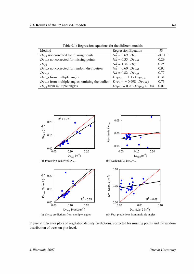
9.3. Results of the PI and VAI models 62
Table 9.1: Regression equations for the different modelsMethod Regression Equation R2
DvPI not corrected for missing points Nd = 0.69 · DvP -0.81DvVAI not corrected for missing points Nd = 0.35 · DvVAI 0.29DvPI Nd = 1.34 · DvP 0.25DvVAI not corrected for random distribution Nd = 0.60 · DvVAI 0.93DvVAI Nd = 0.82 · DvVAI 0.77DvVAI from multiple angles DvVAI,1 = 1.1 · DvVAI,2 0.31DvVAI from multiple angles, omitting the outlier DvVAI,1 = 0.998 · DvVAI,2 0.73DvPI from multiple angles DvPI,1 = 0.20 · DvPI,2 + 0.04 0.07
0.00
0.10
0.20
0.00 0.10 0.20
Dv N
d (
m-1
)
DvVAI (m-1)
R2 = 0.77
(a) Predictive quality of DvVAI
-0.05
0.00
0.05
0.00 0.10 0.20
Resi
duals
Dv V
AI
DvN d (m-1)
(b) Residuals of the DvVAI
0.00
0.10
0.20
0.00 0.10 0.20
Dv V
AI S
can 1
(m
-1)
DvVAI Scan 2 (m-1)
R2 = 0.35
(c) DvVAI predictions from multiple angles
0.00
0.05
0.10
0.00 0.05 0.10
Dv P
Sca
n 1
(m
-1)
DvP Scan 2 (m-1)
R2 = 0.07
(d) DvPI predictions from multiple angles
Figure 9.5: Scatter plots of vegetation density predictions, corrected for missing points and the randomdistribution of trees on plot level.
J. Warmink, 2007 Utrecht University

9.3. Results of the PI and VAI models 63
The DvVAI predictions from the 9 scans were combined to create a 2D map of the vegetationdensity at breast height (figure 9.6). The polar grid cells with the DvVAI value per scan were plotted inthe forest area. Subsequently, an inverse distance weighted interpolation was used to calculate the DvVAI
value in a square grid with cell sizes of 2x2 m. The resulting grid was clipped to fit the boundaries of thescanned forest. The northern part of the forest was not covered by the laser scans. The south–westernedge of the forest patch show up as a denser part, which was observed in the field.
Figure 9.6: Spatial distribution of vegetation density at breast height (DvVAI) of the forest patch (left)and aerial photograph (right). Dense forest edges show up along the south–western edge
J. Warmink, 2007 Utrecht University

Chapter 10
Accuracy and objectivity of the terrestriallaser scanning method
The results show that the VAI model, corrected for missing points was a good predictor for the aggre-gated vegetation density. The predicted DvVAI for different scans, omitting one outlier, show a strongcorrelation and the regression line matched the line of identity, which indicated a reasonably goodrepeatability of the method. The field measurements and the calculation of the PI van VAI values in-cluded some inaccuracies and parameters, which were studied. The accuracy, objectivity and field timeof the terrestrial laser scanning method will be discussed in this chapter.
10.1 Accuracy of the field data
Accuracy of the reference data
The locations of the trees in the stem map and the locations of the scan positions were measured usingthe tacheometer and had an accuracy of 10 cm. The inaccuracy was caused by manually holding thereflector at the location of the trees and the accuracy of the positioning of the tacheometer. The error inthe location of the trees on the stem map may result in uncertainties in the DvNd value for the referenceplots. The uncertainty of the stem map and the errors in georeferencing between the point cloud andthe stem map, may cause a single tree to be included in the reference plot, but excluded in the modelcalculation. This error is increasingly important in open parts of the forest, when a single tree has alarge influence on the resulting DvNd value. The size of the reference plots, however, was between 10and 75 m2 and a small error in the location of the plot may result in a large error of the DvNd, especiallyfor the small plots.
Resolution of the scan data
The resolution of the scanner was set between 238 and 656 pulses per radial horizontally and between414 and 1104 vertically. In this study, the influence of the resolution of the scan data on the predictivequality of the model was not assessed. Some remarks, however, can be made in this respect:
1. A higher resolution will probably increase the penetrating capacity. Consequently, a larger areacan be covered by a single scan, because more points are available at larger distances.
64

10.2. Accuracy of the density calculation 65
2. A higher resolution will give a better representation of the density, because smaller objects willbe recognized. Table 8.2 shows the spacing between the points at 20 meter distance from thescanner. At the lowest resolution a tree with a diameter of 4.6 cm can be missed by the scanner.
10.2 Accuracy of the density calculation
The Digital Terrain Model of the forest was created by taking the minimal height of the laser points foreach square grid cell of 0.5x0.5 m. The extreme values were filtered out by taking the average valuesfor each 9x9 window. This method is simple, but was seemed sufficient for calculating the averageheight of ground level in the scan area. The inaccuracy in the height where reference data was collected(breast height = 1.3 m ± 10 cm) was larger than the inaccuracy in the DTM. These inaccuracies hadlittle influence on the results, because there was little variation in the diameter in the height interval ofuncertainty around breast height.
Reconstruction of missing points
The point density is an important parameter in the determination of the Dv values. It determines thetheoretical number of pulses that went through a cell (equation 8.3). The percentage of missing pointswas calculated by subtracting the recorded points from the total number of emitted pulses, divided bythe total number of emitted pulses. The percentage of missing points in the point clouds varied between0.5 and 4.1 percent, but introduced a large error in the predicted density values. A possible explanationis that most missing points were located in the height interval of the slice. At breast height, fewer sidebranches and leaves were present, than in the crown of the forest or the ground surface (figure 9.1(a)and 9.1(c)).
Inaccuracies caused by the polar grid
The use of the polar grid introduced uncertainty in the prediction of the density values for the referenceplots. The DvPI and DvVAI values on plot level were determined by averaging the centres of the polarcells that fall inside the plot area (figure 10.1). This caused uncertainty, because the cell boundariesdid not match the plot boundaries. For all cells close to the borders of the reference plot, the cell valuewas only included in the calculation of the reference data if the centre was covered by the referenceplot. Due to this uncertainty, a tree (or part of a tree) inside the reference plot, may be excluded in thecalculation of the DvVAI value. This effect is larger at large distance to the scanner, because the polargrid cells represent a larger surface area, up to 0.9 m2 at 25 meter distance. A possible solution is tomatch the borders of the reference plots to the polar grid cells. This is, however, only possible for asingle scan position, because the locations of the polar grid cells are different for each scan.
The polar shape of the grid was introduced, because the calculations were more easy. The polargrid, however, resulted in uncertainties in the prediction, which increased with distance to the scanner.These uncertainties are caused by the central projection of the laser pulses, which resulted in similarproblems as described by the centrally projected photographic method (section 3.4). Therefore, thelargest disadvantage of the laser scanner is the radial emission of the pulses. A parallel laser scanmethod can solve these problems and make the calculation more easy and accurate. In future studiesit is recommended to use a square grid instead or to resample the polar grid to a square grid beforecomparison. A square grid makes it possible to match the borders of the grid cells with the reference
J. Warmink, 2007 Utrecht University

10.3. Parameters in the terrestrial laser scanning method 66
plots and makes a comparison between the different scans possible on cell level. Furthermore, thevertical variation in vegetation density will probably be more easily introduced on a square grid.
Figure 10.1: The point in polygon operation: the DvVAI and DvPI value of the reference plot wascalculated by averaging the DvVAI and DvPI values of the cells, which centres (represented by thepoints) fall inside the plot area
10.3 Parameters in the terrestrial laser scanning method
Penetrating capacity and cutoff value
During the field measurements, the penetrating capacity of the scanner was lower than expected. Figure10.2 shows the decrease of the number of points in the slice with distance to the scanner. The first fewmeters contain no points, because the scanner was placed at an open area in the forest. Figure 10.2(a)shows that the first trees were located at 7.5 meter. Figure 10.2(c) shows the histogram of scan 8, wherealmost all points were captured in the first meters. In all histograms a rapid decrease with distance, afterthe first peak is visible.
Calculation parameters
The only parameters that were chosen in the calculation, were the size of the cells in the polar grid, thecutoff value and the height of the slice. The cell size was chosen to be about 0.5x0.5 meter at 7 meterdistance to the scanner. The height of the slice was chosen to contain enough points at larger distances.In future studies other shapes and sizes of the grid cells can be studied. The other parameters neededin the calculation were the locations of the scan positions, the point density and the ground elevation atthe position of the scanner. These parameters were measured in the field. Because few decisions weremade by the observer, the calculation of the DvVAI had a high degree of objectivity.
J. Warmink, 2007 Utrecht University

10.3. Parameters in the terrestrial laser scanning method 67
010002000300040005000600070008000
0 5 10 15 20 25
Nu
mb
er
of
po
ints
Distance to scanner (m)
(a) Scan 1
05000
100001500020000250003000035000400004500050000
0 5 10 15 20 25
Nu
mb
er
of
po
ints
Distance to scanner (m)
(b) Scan 2
0
5000
10000
15000
20000
25000
30000
35000
0 5 10 15 20 25
Nu
mb
er
of
po
ints
Distance to scanner (m)
(c) Scan 8
Figure 10.2: Histograms of the number of points (vertical) and the distance to the scanner (horizontal).A large number of points was captured by the first trees visible to the scanner. Afterwards a rapiddecrease in the number of points is visible
Prediction models
The VAI model, corrected for missing points and the random distribution of trees proved to be a betterpredictor for vegetation density than the PI model. The VAI model, however, assumed that Nd2 waslarge. When a large percentage of the pulses was captured in a cell, the ratio between Nd1 and Nd2became very large. This resulted in a very large value for the DvVAI . When all points were captured in acertain cell, Nd2 became zero. This resulted in an infinite value for the DvVAI and the cell was not takeninto account in the computation of the DvVAI for the reference plot. When the cell sizes are small, atree can cover multiple cells at the same distance, and all points are captured, resulting in infinite DvVAI
values. This effect can explain the sensitivity of the VAI model for missing points. When the missingpoints are reconstructed, the number of cells with a infinite value are reduced and more cells are usedto calculate the DvVAI of the reference plot. The PI model was less sensitive to this effect, but did nottake occlusion into account and, therefore, performed less.
After the correction for missing points there were negative values for Nd1 and Nd2 present in thepolar grid. These negative values resulted in an infinite value of DvVAI . These negative values show upfor cells behind dense clusters of trees. Here, number of pulses through a cell was close the theoreticalnumber of pulses through the cell (Ntot). Small errors in Ntot (equation 8.3) could lead to negativevalues. Another explanation for the negative values is that Ntot is overestimated, due to the fixed cellboundaries. Ntot is calculated based on the average number of pulses that went through a cell. Theactual number of points through a cell, however, can be larger when the cell boundaries are narrowlyfixed around the laser pulses. Figure 10.3 shows that the actual pulse density (number of pulses insidethe red rectangle divided by the surface area) is larger than the average pulse density (number of pulsesinside the blue rectangle divided by the surface area; equation 8.3), for the same number of points.The average pulse density calculated for the area inside the red rectangle is, therefore, smaller than theactual pulse density. When, in this case, all pulses are recorded in a single cell, the calculated Nd2 issmaller than zero. Likewise, the Ntot can be the underestimated when the cell boundaries are narrowlyfixed inside the laser pulses, resulting in an overestimation of Nd2. This will, however, not result in aninfinite value of DvVAI and the cell will be included in the computation of the DvVAI for the referenceplot. Because, at plot level multiple cells are averaged to compute DvVAI , the random overestimationof Nd2 will have little influence.
J. Warmink, 2007 Utrecht University

10.4. Objectivity and time requirements of the TLS method 68
Figure 10.3: Explanation for a negative number of points after the proximal or distal cell boundary. Thepoints represent the laser pulses, the red rectangle shows the cross section of the a distal cell boundaryin the direction of the laser pulses and the blue rectangle shows the surface area represented by theaverage pulse density, for the number of pulses through the distal cell boundary.
10.4 Objectivity and time requirements of the TLS method
In the previous sections is shown that the accuracy of the TLS method depended on the accuracy of thefield measurements and the averaging of the DvPI and DvVAI values per cell to predict the density atplot level. The radial emission of the laser pulses resulted in large “shadows”, where no points wererecorded. Due to the averaging of the polar cells in the plot areas, uncertainties were caused, becausecells with infinite DvVAI values or zero DvPI values occurred in the “shadow” areas. The VAI modelgave the best result for the reference plot (R2 = 0.77) with a slope of the regression line of 0.82. Whenthe DvVAI predictions for the reference plots were compared for different scan positions (figure 9.5(c)),31 percent of the variance was explained by the regression line. However, when one outlier was omitted,the R2 value increased to 0.73 with a slope of the regression line of 0.998. This indicated a reasonablyhigh repeatability of the method. Regression analysis on the predicted DvPI , however, explained littlevariance (R2 = 0.25), because no correction for occlusion was included in the model.
The choices made in the TLS method were: (1) the decision for the cell sizes of the polar grid, (2)the height of the slice, and (3) the cutoff value, which was mainly determined by the penetrating capacityof the laser scans. The two random effects which influenced the results were: (1) the inaccuracy in thedetermination of the locations of the trees, which can cause a tree to be excluded from the reference plot,but included in the DvVAI prediction on plot level and (2) the under or overestimation of Ntot, whichresulted in an erroneous, real number for Nd1 and Nd2. In the calculation of the vegetation density,few arbitrary decisions were made. The assumptions underlying the method were that: the trees wererandomly distributed, all laser pulses were recorded, and the pulses travelled parallel through the forest.Because of the small cells in the polar grid, parallel pulses were assumed, the missing points werereconstructed and the a correction for the random distribution of the trees was included on plot level.
A disadvantage of the terrestrial laser scanning method was that field measurements were costlycompared to the photographic method and manual methods, because laser scanning equipment is ex-pensive. For this research, a specialized company had to be hired to conduct the scanning. Furthermore,collecting the laser scan data in the field was time consuming. In one day, 8 laser scans were made,
J. Warmink, 2007 Utrecht University

10.4. Objectivity and time requirements of the TLS method 69
covering tree quarters of a relatively open forest. The resulting data acquired by this method, however,was very detailed and spatially variable. Instead of the time of flight type scanner, used in this research aphase–based scanner (section 3.5.1) can be used. This type of scanner is less accurate and has a limitedrange (100m), but the penetrating capacity in the forest was only 25 meter in this study. The advantageof the phase–based scanner is that it is much faster than a time of flight scanner.
The amount of data resulting from a single scan was around 3.5 million points. This resulted ina significant calculation time. The use of the slice approach reduced the number of points needed forcalculation from 3.5 million to 200000 per scan. The calculation time was, thereby, reduced from 3hours per scan to 10 minutes. The time needed for the total data analysis was about 3 hours, but can bereduced by optimizing the algorithm. The data analysis was fully automated and needed no interactionof the surveyor.
J. Warmink, 2007 Utrecht University

Chapter 11
Comparison of parallel photography andterrestrial laser scanning
In this research several methods were discussed to measure the hydrodynamic vegetation density in thelowland floodplains. The TLS method was applied in a floodplain softwood forest and the CP and PPmethod were applied to various vegetation types. In this chapter the application and the strengths andweaknesses of the different methods are compared.
11.1 Accuracy of the methods
The manual method used for collecting reference data, was applicable on forest plots with few sidebranches. This method was based on the assumption of cylindrical vegetation. Inaccuracies werecaused by the decision of the measurement height. For plots with complex vegetation, the measurementerrors were significant and the method was not applicable, because the assumption was not valid. Forthe validation plots, the manual method seems accurate. This should be tested by multiple inventoriesof the same plot.
The parallel photographic method performed equally well as the manual method for the valida-tion plots (R2 = 0.996) and the regression line matched the line of identity. Because the manual methodwas an accurate measurement technique for vegetation density of cylindrical vegetation, it was con-cluded that the PP method had a very high accuracy. The PP method does not depend on the underlyingassumption of the manual method and, therefore, can be applied on more complex vegetation types.The inaccuracies in the resulting DvPP values were mainly caused by the measurement error of the plotlength in the field and errors in the classification of the pixels.
The terrestrial laser scanning method performed well for the prediction of the vegetation den-sity in the studied forest. The VAI corrected for missing points and the random distribution of treesexplained 77 percent of the field variance. The slope of the regression line was 0.82 and significantlydiffered from 1. PI, corrected for missing points explained little variance (R2 = 0.25), because nocorrection for occlusion was included in the model. The averaging of the DvPI and DvVAI values forthe reference plots included uncertainty in the method.
The PP method, therefore, is a more accurate method to measure the vegetation density at plotlevel, while the TLS method is more efficient to map 2D distribution.
70

11.2. Objectivity of the methods 71
11.2 Objectivity of the methods
DvNd lacks objectivity for complex vegetation, because a decision has to be made, which stems areselected to measure the diameter. The decisions that had to be made using the PP method were theheight and distance of the camera to the plot and the camera settings (resolution, opening angle andexposure). The resulting DvPP proved sensitive to the resolution of the photographs, which must beset as high as possible for complex vegetation. The threshold on the intensity histogram has a certaindegree of subjectivity, depending on the contrast of the initial photographs. The threshold on the huehistogram needs calibration, but depends only on the color of the screen.
For the TLS method, few arbitrary decisions were made during the measurement and the dataanalysis. The decisions made by the researcher were the choice of the type of calculation grid and thelocations and resolution of the scans. The consequences of changes in the grid or resolution were notstudied in this research. Further research is needed to investigate the influence of these parameters onthe vegetation density predictions. Overall can be said that the PP and TLS method have a high degreeof objectivity.
11.3 Time and equipment needed for the methods
Besides the accuracy and objectivity of the methods, the time and equipment needed to carry out thefield measurements determined the applicability of the methods. The advantage of the manual methodwas that only a notebook, tape measure and sliding gauge were needed in the field. The PP methodneeded a lot of equipment (section 5.2.1), thereby reducing the accessibility in complex vegetation. Forthe TLS method a lot of advanced equipment was needed. This made the method expensive comparedto the other two methods.
Besides the price of the equipment, the costs of a method are determined by the time needed inthe field and for data analysis. The time needed for the field measurements was difficult to compare,because the methods have different support. The manual method took about 5 minutes for a forest plot,but the measurement time increased to 45 minutes for complex vegetation. The PP method methodtook about 30 minutes, which was independent of the complexity of the vegetation. Including the timefor relocation, an experienced surveyor can measure 8 to 10 plots per day. When fewer pictures weretaken per plot, which had a minimal effect on the vegetation density prediction (section 7.3.2), the fieldtime decreased, down to 10 minutes. A further decrease of the time in the field can be achieved byimproving the field equipment. This can reduce the time to setup the screen and rail, significantly. Thetime needed for the data analysis of the parallel photograph method is minimal, when automated.
The data collection of the laser data was done in one day (8 hours) and 9 laser scans were made.Creating the dGPS points around the forest took about 4 hours. The 9 scans covered three quarters ofa forest of 120x80 meters. The laser scanner can cover, in the same amount of time, a larger area thanthe PP method, but a coordinate system is needed in the study area. The time required in the field canbe reduced using a phase–based scanner. The data analysis for the TLS method was more complicatedand time consuming than for the PP method. Delfttech, the company responsible for post processingthe raw laser data, used about three days for georeferencing. The calculation of the DvVAI value for thescans took about 90 minutes of computer time, but can be fully automated.
J. Warmink, 2007 Utrecht University

11.4. Application of the methods in the field 72
Table 11.1: Strengths and weaknesses of the different methods (++ = very positive, ◦ = neutral and −−= very negative)
Nd method PP method CP method TLS VAI TLS PIAccuracy forest ++ ++ ◦ + −−
herbs −− ++ ◦Objectivity forest + + ◦ + +
herbs −− ++ +
Equipment + − ◦ −− −−Field Time ◦ − + − −Analysis Time + + − − −Spatial Variability − − − ++ ◦
11.4 Application of the methods in the field
The advantages and disadvantages of the methods are summarized in table 11.1. The manual method isan appropriate measurement method when the assumption underlying the method is valid. It is an easyand fast method to measure the vegetation density of forests, with little side branches and leaves.
The strongest point of the TLS method is the spatial variability of the vegetation density mea-surements. The method proved to be accurate, although less than the PP method, without the need forcalibration and had a high degree of objectivity (section 11.2). Therefore, it was concluded that theTLS method is an appropriate measurement method for measuring aggregated vegetation density data.
The parallel photographic method proved to be a reliable tool to measure accurate and objectivefield data without the need for calibration. This data can be used as input data for the ecotope approachor as reference data for airborne laser scanning or other methods, which need calibration. The PPmethod was the only method in this research, which can objectively measure herbaceous vegetation.The equipment must be adapted, to measure vegetation lower than 0.5 meter. When no spatial variabilityis needed, the PP method will produce the best results.
J. Warmink, 2007 Utrecht University

Chapter 12
Conclusions and recommendations
12.1 Conclusions
The aim of this research was to develop a photographic method and terrestrial laser scanning on flood-plain vegetation to determine the vegetation density for hydrodynamic roughness calculations. In thisresearch, the parallel photographic method and the terrestrial laser scanning method, both based on theoptical point quadrat method, were used to quantify the hydrodynamic vegetation density of floodplainvegetation. The manual method, where the Dv was calculated by multiplying the average diameter bythe number of stems per square meter, was used as validation data.
12.1.1 Parallel photography
In this thesis, a new measurement tool was developed: the parallel photographic method (PP), whichpredicts the vegetation density very well (R2 = 0.996) up to vegetation densities of 0.12 (m−1), whichis dense forest, without the need for calibration. The PP method was an improvement of the centralphotographic method (R2 = 0.87). The PP method consists of the computation of the fractional cover-age of vegetation against a contrasting background on a digital photo mosaic of parallel images. Thediameters of individual trees measured in the field were reconstructed on the parallel photo mosaic andshowed an R2 of 0.97.
The PP method was applied on more complex vegetation and gave consistent results. The methodused to measure herb vegetation gave the best results using a red screen and apply the threshold on thehue value of the photographs. PP is an accurate and objective measurement tool for the hydrodynamicvegetation density of floodplain vegetation. The method is applicable on summer and winter vegetation.
Some remarks on the methodology of the PP method are:
• Measured density values range from 0.01 m−1 for open forest, to 6.17 m−1 for the lower layer ofa herb plot.
• The method took about 25 minutes per plot and a lot of equipment was needed, thereby reducingthe accessibility in dense vegetation. The time needed for the data analysis was 5 minutes.
• The accuracy of DvPP was mainly determined by inaccuracies in the plot length measurementsin the field and the resolution of the photographs.
• The spacing between the photographs needed to create a parallel photo mosaic, producing accu-rate results, was 20 cm for the studied forest plot and 10 cm for the herb plot.
73

12.2. Recommendations 74
• On plot level, the PP method outperformed terrestrial laser scanning.
12.1.2 Terrestrial laser scanning
In this thesis, a second new method is presented to extract the aggregated vegetation density fromterrestrial laser scanning (TLS) data for application in hydraulic models. Two different models weretested to predict the vegetation density: (1) the Percentage Index (PI) and (2) the Vegetation Area Index(VAI). The results show that:
• The PI model was a bad predictor for the vegetation density for the reference plots (R2 = 0.25).• The VAI model gave the best predictions for the reference plots (R2 = 0.77).• Correction for missing point and the assumptions of the random distribution of trees is required.• No calibration is required for the VAI model.• The presented method has a high degree of objectivity.
Some remarks on the methodology of the TLS method are:
• The accuracy of the DvVAI on plot level was mainly determined by inaccuracies caused by theaveraging of the DvVAI values per cell.
• The radial emission of the laser pulses resulted in increasingly large areas where no data wascollected.
• Time required for the data analysis and the field time was 2 and 8 hours respectively, for 9 scanscovering three quarters of the studied forest.
• Using the slice approach, the 2D VAI method can easily be extended to 3D using multiple slices.• The VAI model provide surveyors with a new methods for accurate vegetation density field mea-
surements: averaged over a plot or spatially variable.
12.2 Recommendations
12.2.1 Parallel photography
For future research using the PP method some recommendations are:
• Improve the guide rail and screen setup to reduce field time.• When low vegetation is measured, the equipment needs to be improved by decreasing the height
of the tripods.• Using a collapsible board as background instead of the screen will reduce differences in illumi-
nation.• A frame around the plot area reduces distortions of the plot and increases the accuracy of the plot
length measurement.• Fewer photographs are needed to create a representative parallel photograph of woody vegetation.• A blue or purple background will probably improve the discrimination between screen and veg-
etation by the hue threshold.• The resolution of the photographs has a large influence on DvPP. The optimal resolution is of
interest to future research.
J. Warmink, 2007 Utrecht University

12.2. Recommendations 75
12.2.2 Terrestrial laser scanning
Some recommendations for future research are:
• The laser scans should be made from inside the forest, the edge of the studied forest was toodense to penetrate.
• Use a phase–based scanner instead of the time of flight scanner, to increase point density andreduce scan time.
• An increased scan resolution will increase the penetrating capacity of the scanner. The optimalresolution of the scanner is of interest to future research.
• The slice and polar grid approach show limitations. A square calculation grids might give betterresults, but is more complicated.
• In this study a single slice around breast height was used. The method can be expanded withmultiple slices, to determine the vertical variation in vegetation density of the forest.
• Future studies are needed to test the applicability of terrestrial laser scanning on more complexvegetation.
When measurements of the spatial variability of the vegetation density is required, the terrestriallaser scanning method gives good results. It is recommended to use the parallel photographic methodas calibration data, especially, for herb vegetation and as density values of herb vegetation used for theecotope approach. It is concluded that TLS and PP are two complementary techniques, that show highaccuracies for field measurements of vegetation density.
J. Warmink, 2007 Utrecht University

References
Aber, J. D., 1979. A method for estimating foliage-height profiles in broad-leaved forests. Journal ofEcology 67, 35–40.
Anonymous, december 1995. Wet op de waterkering. Tech. rep., Ministry of Transportation, Publicworks and Water management, The Hague, The Netherlands, (in Dutch).
Anonymous, 2004. 4e voortgangsrapportage ”ruimte voor de rivier” januari-juni 2004. Tech. rep., Min-istry of Transport, Public works and Water management, The Hague, The Netherlands, (in Dutch).
Aschoff, T., Thies, M., Spiecker, H., 2004. Describing forest stands using terrestrial laser–scanning. In:Thies, M., Koch, B., Spiecker, H., Weinacker, H. (Eds.), Proceedings of the ISPRS working groupVIII/2: ‘Laser-Scanners for Forest and Landscape Assessment’. International Society of Photogram-metry and Remote Sensing.
Baptist, M. J., 2005. Modelling floodplain biogeomorphology. Ph.D. thesis, Delft University of Tech-nology, Delft University Press, Delft.
Baptist, M. J., Penning, W. E., Duel, H., Smits, A. J. M., Geerling, G. W., van der Lee, G. E. M.,Alphen, J. S. L. V., 2004. Assessment of the effects of cyclic floodplain rejuvenation on flood levelsand biodiversity along the rhine river. River Research and Applications 20, 285–297.
Besl, P. J., McKay, N. D., 1992. A method for registration of 3–d shapes. IEEE transitions on patternanalysis and machine intelligence 14 (2), 239–256.
Bienert, A., Maas, H., Scheller, S., 2006. Analysis of the information content of terrestrial laserscannerpoint clouds for the automatic determination of forest inventory parameters. In: T. Koukal, W. S.(Ed.), Proceedings International Workshop 3D Remote Sensing In Forestry. pp. 44–49.
Bridge, J. S., 2003. Rivers and floodplains. Forms, processes and sedimentary record. Blackwell Pub-lishing, Malden, USA.
Chasmer, L., Hopkinson, C., Treitz, P., 2004. Assessing the three–dimensional frequency distribution ofairborne and ground–based laser lidar data for red pine and mixed deciduous forest plots. In: Thies,M., Koch, B., Spiecker, H., Weinacker, H. (Eds.), Proceedings of the ISPRS working group VIII/2:‘Laser-Scanners for Forest and Landscape Assessment’. International Society of Photogrammetryand Remote Sensing.
Cobby, D. M., Mason, D. C., Davenport, I. J., 2001. Image processing of airborne scanning laseraltimetry data for improved river flood modelling. ISPRS Journal of Photogrammetry and RemoteSensing 56, 121–138.
76

REFERENCES 77
Dudley, S. J., Bonham, C. D., Abt, S. R., Fischenich, J. C., 1998. Comparison of methods for measuringwoody riparian vegetation density. Journal of Arid Environments 38, 77–86.
Duel, H., Baptist, M. J., Penning, W. E., 2001. Cyclic floodplain rejuvenation: a new strategy based onfloodplain measures for both flood risk managemant and enhancement of the biodiversity of the riverrhine. Tech. Rep. NCR report 14-2001, NCR, Delft.
Ehlers, M., Gahler, M., Janowsky, R., 2003. Automated analyses of ultra high resolution remote sensingdata for biotope mapping: new possibilities and challenges. ISPRS Journal of Photogrammetry andRemote Sensing 57, 315–326.
Fathi-Maghadam, M., Kouwen, N., 1997. Nonrigid, nonsubmerged, vegetative roughness on flood-plains. Journal of Hydraulic Engineering, ASCE 123, 51–57.
Fishenich, J. C., 1996. Hydraulic impacts of riparian vegetation. computation of resistance. Tech. Rep.EL–96–XX, EMRRP, U.S. Army Corps of Engineers Waterways Experiment Station.
Frohlich, C., Mettenleiter, M., 2004. Terrestrial laser scanning – new perspectives in 3d surveying. In:Thies, M., Koch, B., Spiecker, H., Weinacker, H. (Eds.), Proceedings of the ISPRS working groupVIII/2: ‘Laser-Scanners for Forest and Landscape Assessment’. International Society of Photogram-metry and Remote Sensing.
Gorte, B. G. H., Winterhalder, D., 2004. Reconstruction of laser–scanned trees using filter operations inthe 3d raster domain. In: Thies, M., Koch, B., Spiecker, H., Weinacker, H. (Eds.), Proceedings of theISPRS working group VIII/2: ‘Laser-Scanners for Forest and Landscape Assessment’. InternationalSociety of Photogrammetry and Remote Sensing.
Greame, D., Dunkerley, D. L., 1993. Hydraulic resistance by the river red gum, eucalyptus carnaldu-lensis, in ephemeral desert streams. Australian Geographic Studies 31 (2), 141–154.
Jans, L., 2004. Evaluatie nevengeulen gamerensche waard 1996-2002. Tech. Rep. 2004.024, Rijksinsti-tuut voor Integraal Zoetwaterbeheer en Afvalwaterbehandeling / RIZA, Arnhem, (in Dutch).
Jansen, B. J. M., Backx, J. J. G. M., 1998. Ecotopenkartering rijntakken–oost 1997. Tech. Rep.98.054, Rijksinstituut voor Integraal Zoetwaterbeheer en Afvalwaterbehandeling / RIZA, Lelystad,(in Dutch).
Jarvela, J., 2002. Determination of flow resistance of vegetated channel banks and floodplains. In:Bousmar, D., Zech, Y. (Eds.), River Flow 2002. Swets and Zeitlinger, Lisse, pp. 311–318.
Jarvela, J., 2004. Determination of flow resistance caused by non–submerged woody vegetation. Inter-national Journal of River Basin Management 2 (1), 61–70.
Jesse, P., april 2004. Hydraulische weerstand in (natuur) ontwikkeling: de verandering van de hydraulis-che ruwheid van acht natuurontwikkelingsprojecten. Tech. Rep. 2003.124X, Rijksinstituut voor In-tegraal Zoetwaterbeheer en Afvalwaterbehandeling / RIZA, Arnhem, (in Dutch).
Jonckheere, I., Fleck, S., Nackaerts, K., Muys, B., Choppin, P., Weiss, M., Baret, F., 2004. Reviewof methods for in situ leaf area index determination: Part I. theories, sensors and hemisphericalphotography. Agricultural and Forest Meteorology 121, 19–35.
J. Warmink, 2007 Utrecht University

REFERENCES 78
Klopstra, D., Barneveld, H. J., van Noortwijk, J. M., van Velzen, E. H., 1997. Analytical model forhydraulic roughness of submerged vegetation. In: Proceedings of theme A, managing water: copingwith scarcity and abundance. American Society of Civil Engineers (ASCE), pp. 775–780.
Kouwen, N., Fathi-Moghadam, M., 2000. Friction factors for coniferous trees along rivers. Journal ofHydraulic Engineering 126 (10), 732–740.
Kouwen, N., Li, R.-M., 1980. Biomechanics of vegetative channel linings. Journal of Hydraulics Devi-sion ASCE 106 (6), 1085–1103.
Kraus, K., Rieger, W., 1999. Processing of laser scanned data wooded areas. In: Fritsch, D., Spiller, R.(Eds.), Photogrammetric Week ’99’. pp. 221–231.
Lefsky, M. A., Cohen, W. B., Parker, G. G., Harding, D. J., 2002. Lidar remote sensing for ecosystemstudies. Bioscience 52 (1), 19–30.
Leica Geosystems, 2006. http://www.leica-geosystems.com. accessed on 31 January 2006.
Lemmens, M. J. P. M., van den Heuvel, F. A., 2001. 3d close–range laser mapping systems. GIMInternational 15 (1), 30–33.
Levy, E. B., Madden, E. A., 1933. A point method of pasture analysis. Journal of Agriculture 46, 267–279.
Lichti, D., Gordon, D. J., Stewart, M. P., 2002. Ground–based laser scanners: operation, systems andapplication. Geomatica 56 (21–33).
Lillesand, T. M., Kiefer, R. W., Chipman, J. W., 2004. Remote sensing and image interpretation, fifthedition Edition. John Wiley and Sons, Inc., New York, USA.
MacArthur, R. H., Horn, H. S., 1969. Foliage profile by vertical measurements. Ecology 50 (5), 802–804.
MacArthur, R. H., MacArthur, J. W., 1961. On bird species diversity. Ecology 42 (3), 594–598.
Marks, K., Bates, P., 2000. Integration of high resolution topographic data with floodplain flow models.Hydrological Processes 14 (11–12), 2109–2122.
Mason, D. C., Cobby, D. M., Horrit, M. S., Bates, P., 2003. Floodplain friction parameterization intwo-dimensional river flood models using vegetation heights derived from airborne scanning laseraltimetry. Hydrological Processes 17, 1711–1732.
MeVisLab, 2006. http://www.mevislab.de. accessed on 10 July 2006.
Middelkoop, H., van Asselt, M. B. A., van ’t Klooster, S. A., van Deursen, W. P. A., Kwadijk, J. C. J.,Buiteveld, H., 2004. Perspectives on flood management in the rhine and meuse rivers. River Researchand Applications 20, 327–342.
Nepf, H. M., 1999. Drag, turbulence, and diffusion in flow through emergent vegetation. Water Re-sources Research 35 (2), 479–489.
Nienhuis, P. H., A. D. Buijse, R. S. E. W. Leuven, A. J. M. S., de Nooij, R. J. W., Samborska, E. M.,2002. Ecological rehabilitation of the lowland basin of the river rhine (nw europe). Hydrobiologia478, 53–72.
J. Warmink, 2007 Utrecht University
REFERENCES 79
Niklas, K. J., Moon, F. C., 1988. Flexural stiffness and modulus of elasticity of flower stalks from alliumsativum as measured by multiple resonance frequency spectra. Am. Journal of Botany 75 (10), 1517–1525.
Nobis, M., Hunziker, U., 2005. Automatic thresholding for hemispherical conpy-photographs based onedge detection. Agricultural and Forest Meteorology 128, 243–250.
Parker, G. G., Harding, D. J., Berger, M. L., 2004. A portable system for rapid determination offorest canopy structure. Journal of Applied Ecology 41, 755–767.
Petryk, S., Bosmajian, G., 1975. Analysis of flow through vegetation. Journal of Hydraulics Divisions101, 871–884.
Rademakers, J. G. M., Wolfert, H. P., 1994. Het rivier-ecotopen-stelsel: een indeling van ecologischrelevante ruimtelijke eenheden ten behoeve van ontwerp– en beleidsstudies in het buitendijkse riv-ierengebied. Tech. Rep. 61-1994, Rijksinstituut voor Integraal Zoetwaterbeheer en Afvalwaterbehan-deling / RIZA, Lelystad, (in Dutch).
Ritzen, M., Straatsma, M., 2002. Laseraltimetrie en hydraulische vegetatieruwheid van uiterwaarden.Master’s thesis, Universiteit Utrecht, (in Dutch).
Roebertsen, H., Heil, G. W., Bobbink, R., 1988. Digital picture processing: a new method to analysevegetation structure. Acta Botanica Neerlandica 37 (2), 187–192.
Shi, Z., Hughes, J. M. R., 2002. Laboratory flume studies of microflow environments of aquatic plants.Hydrological Processes 16, 3279–3289.
Smits, A. J. M., Havinga, H., Marteijn, E. C. L., 2000. New concepts in river and water managementin the rhine river basin: how to live with the unexpected? In: Smits, A. J. M., Nienhuis, P. H.,Leuven, R. S. E. W. (Eds.), New Approaches to River Management. Backhuys Publishers, Leiden,pp. 267–286.
Straatsma, M. W., 2005. Quantitative mapping of hydrodynamic vegetation density of floodplain forestsusing airborne laser scanning. In: The International Archives of the ISPRS. Vol. 36. Part 3/W19.
Straatsma, M. W., Middelkoop, H., 2006. Airborne laser scanning as a tool for lowland floodplainvegetation monitoring. Hydrobiologia 565, 87–103.
Straatsma, M. W., Warmink, J., Middelkoop, H., submitted. Two novel methods for field measurementsof hydrodynamic vegetation density of floodplain vegetation using terrestrial laser scanning and dig-ital parallel photography. Submitted to: International Journal of Remote Sensing. Special issue: 3DRemote Sensing in Forestry.
The Gimp 2.2, 2006. http://www.gimp.org. accessed on 31 January 2006.
Thies, M., Pfeifer, N., Winterhalder, D., Gorte, B. G. H., 2004. 3d–reconstruction of stems for ta-per, sweep and lean assessment based on laser scanning of standing trees. In: Thies, M., Koch, B.,Spiecker, H., Weinacker, H. (Eds.), Proceedings of the ISPRS working group VIII/2: ‘Laser-Scannersfor Forest and Landscape Assessment’. International Society of Photogrammetry and Remote Sens-ing.
J. Warmink, 2007 Utrecht University

REFERENCES 80
Van der Sande, C. J., de Jong, S. M., de Roo, A. P. J., 2003. A segmentation and classification approachof IKONOS-2 imagery for land cover mapping to assist flood risk and flood damage assessment.International Journal of Applied Earth Observation and Geoinformation 4, 217–229.
Van Stokkom, H. T. C., Smits, J. M., Leuven, R. S. E. W., 2005. Flood defence in the netherlands; a newera a new approach. International Water Resources Association, Water International 30 (1), 76–87.
Van Velzen, E. H., Jesse, P., Cornelissen, P., Coops, H., 2003a. Stromingsweerstand vegetatie in uiter-waarden: deel 1 handboek. Tech. Rep. RIZA rapport 2003.028, Rijksinstituut voor Integraal Zoetwa-terbeheer en Afvalwaterbehandeling / RIZA, Arnhem, (in Dutch).
Van Velzen, E. H., Jesse, P., Cornelissen, P., Coops, H., November 2003b. Stromingweerstand vegetatiein uiterwaarden: deel 2 achtergronddocument. Tech. Rep. 2003.029, Rijksinstituut voor IntegraalZoetwaterbeheer en Afvalwaterbehandeling / RIZA, Arnhem, (in Dutch).
Wijma, E., 2005. Hydraulic roughness of riverine softwood forest. Master’s thesis, Utrecht University.
Zehm, A., Nobis, M., Schwabe, A., 2003. Multiparameter analysis of vertical vegetation structure basedon digital image processing. Flora 198, 142–160.
J. Warmink, 2007 Utrecht University

Appendix A
Maps of the study areas
A.1 Topographic maps of the study areas
A.2 Maps with vegetation classes and measurement locations
Duursche Waarden I
Duursche Waarden II
Gamerensche Waard
TLS forest in the Gamerensche Waard

Topographic maps of the study areas
Topographical map of the Duursche Waard, with the natural reserve area: “Duursche Waarden and the area around Fortmond
Topographical map of the Gamerensche Waard floodplain, with the old brick factory in the centre. The arrow is pointing towards the forest where the tls measurements were conducted

31 30
48
3534
32 2928
49
51
5037
36
27
2625
2423
22
2019
5233
61
6059
58
57
201800
201800
202000
202000
202200
202200
202400
202400
202600
202600
202800
202800
203000
203000
203200
203200
203400
203400
203600
203600
203800
203800
204000
204000
204200
204200
4862
00
4862
00
4864
00
4864
00
4866
00
4866
00
4868
00
4868
00
4870
00
4870
00
4872
00
4872
00
4874
00
4874
00
Fieldmap of the Duursche Waarden: the area around Fortmondwith topographical vegetation descriptions from DTB - River and measurement locations
LegendTopography
hardwood forestsoftwood forestyoung softwood forestshrub vegetationorchardreed marshesnatural grasslandagricultural arealake
Parallel photography plotsvalidation plotsleaved forest plotsherbaceous plotslower layer plotslarge opening anglereed marshgrass plotsomitted plotsplots measured summer and winter
Jord Warmink
0 250 500 750125Meters
January 2007
Fortmond
from: Ministry of Public Works and Transportation:"Digitaal Topografisch Bestand (DTB) RivierMeetkundige Dienst afdeling Topografische GEO-informatie"Version: 3.1 Date of last change: 5 March 1999

31 30
48
47
46
4544
43
3534
32 2928
494238
37
36
27
2625
2423
2241
40
3961
60
59 58
57
202800
202800
203000
203000
203200
203200
203400
203400
203600
203600
203800
203800
204000
204000
204200
204200
204400
204400
204600
204600
204800
204800
205000
205000
205200
205200
205400
205400
205600
205600
205800
205800 4868
00
4870
00
4870
00
4872
00
4872
00
4874
00
4874
00
4876
00
4876
00
4878
00
4878
00
4880
00
4880
00
4882
00
4882
00
4884
00
4884
00
Fieldmap of the Duursche Waarden II: the nature reserve area withtopographical vegetation descriptions from DTB - River and the measurement locations
LegendTopography
hardwood forestsoftwood forestyoung softwood forestshrub vegetationorchardreed marshesnatural grasslandagricultural arealake
Parallel photography plotsvalidation plotsleaved forest plotsherbaceous plotslower layer plotslarge opening anglereed marshgrass plotsomitted plotsplots measured summer and winter
Jord Warmink
0 250 500 750125Meters
January 2007
from: Ministry of Public Works and Transportation:"Digitaal Topografisch Bestand (DTB) RivierMeetkundige Dienst afdeling Topografische GEO-informatie"Version: 3.1 Date of last change: 5 March 1999

9
714
1318 17
12
11103
141600
141600
141800
141800
142000
142000
142200
142200
142400
142400
142600
142600
142800
142800
143000
143000
143200
143200
143400
143400
143600
143600
143800
143800
4236
00
4236
00
4238
00
4238
00
4240
00
4240
00
4242
00
4242
00
4244
00
4244
00
4246
00
4246
00
Fieldmap of the Gamerensche Waard with topographicalvegetation descriptions from DTB - River and measurement locations
LegendTopography
softwood forestyoung softwood forestshrub vegetationherbaceous vegetation
reed marshesorchardlakewater
Parallel photography plotsValidation plotsLeaved forest plotsLower layer plotsLarge opening angleOmitted plot
Jord Warmink
0 250 500 750125Meters
January 2007
from: Ministry of Public Works and Transportation:"Digitaal Topografisch Bestand (DTB) RivierMeetkundige Dienst afdeling Topografische GEO-informatie"Version: 3.1 Date of last change: 5 March 1999

9
7
14
11
103
86
54
2
1
1615
9988
77
66
5544
3322
11
141550
141550
141600
141600
141650
141650
141700
141700
4243
50
4243
50
4244
00
4244
00
4244
50
4244
50
4245
00
4245
00
4245
50
4245
50
Fieldmap of the Gamerensche Waard withtopographical vegetation descriptions from
DTB - River and measurement locations
LegendTopography
softwood forestherbaceous vegetationwater
TLSLaser scan postions
dGPS pickets
Parallel photography plotsValidation plots
Leaved forest plots
Lower layer plots
Large opening angle
Omitted
Jord Warmink
0 25 50 7512,5Meters
January 2007
from: Ministry of Public Works and Transportation: "DigitaalTopografisch Bestand (DTB) RivierMeetkundige Dienst afdelingTopografische GEO-informatie"Version: 3.1 Date of last change: 5 March 1999

Appendix B
Flowcharts and scripts
B.1 Parallel photographic method
Flowchart of the python script to create a parallel photo mosaic
Python script to create a parallel photo mosaic
Flowchart of hue thresholding using MeVisLab
B.2 Terrestrial laser scanning method
Flowchart of the terrestrial laser scanning method
Explanation of the python script to compute DvVAI
Python script to compute DvVAI based on the point cloud

FunctionSelect the centre box out of the original photograph with size:(width, heightpics)
FunctionPaste the selected box in the new picture. And write the mosaic new to the disk
FilesOriginal photographs
FunctionDetermine the number of original photographs (pics)
FunctionCreate new image with size:(width*nrpics, heightpics)
Width value
Parallel Photo Parallel Photo mosaicmosaic
Flowchart of the Python script to create a parallel photo mosaic

2007-01 CreateMosaic.py 1/3
J. Warmink Utrecht University
Python script to create photo mosaic
import os import Image from string import split from os import system from matplotlib.pylab import hist, show, bar, plot, subplot, title, ylabel ### Global module works in ./ # General Flowchart: # create a dirlist --> make piclists --> enter directory--> ## read infofile --> extract plotnr --> ### create the new image and write it to p-photo --> #### write a new infofile [with first line is the number of centre columns] ### General Settings... borders = [[0,56],[57,61]] # Set range of plots-IDs for which the # values are valid (more can be added) format = ['img','dcp'] # The characters to select the photographs # in the folder extension = ['jpg','jpg'] # Set the extension of the photographs target = 'p-photos/' # Photo mosaics are saves to this folder # Function to write the names of the photographs in all plot folder # defined in "dirlist.txt" to a file "piclist.txt" def create_dirlist(borders, format, extension): print 'create_dirlist() started' print 'dirlist created...' for x in file('dirlist.txt','r').readlines(): directory = x[:-1]; plot = split(directory,'_')[1][4:] for i in range(len(borders)): if borders[i][0] <= int(plot[:2]) <= borders[i][1]: ## Execute the bash command to create a file with all ## directories containing photographs command = 'ls -d ./'+directory+'/'+format[i]+'*.'+extension[i]+' | '+directory+'/piclist.txt' os.system(command) print "piclist written in: "+directory fileexists('piclist.txt','dirlist.txt') # Function to check if "filename" exists in the folders named in "folderfile" def fileexists(filename, folderfile): for x in file(folderfile,'r').readlines(): directory = x[:-1] try: open('./'+directory+'/'+filename) continue except: print "ERROR...\nCreate "+filename+" first!\nScript Terminated" break print filename+" exists in all directories listed in "+folderfile return True

2007-01 CreateMosaic.py 2/3
J. Warmink Utrecht University
# Function to write the initial infofile in all folders in "folderfile" def write_ini_info(): for x in file('widths.txt', 'r').readlines(): for directory in file('dirlist.txt','r').readlines(): plot=split(x,'\t')[0] width=split(x,'\t')[1] plot_dir=split(directory[:-1],'_')[1][4:] if plot_dir == plot: write_file(plot,width[:-1],directory[:-1]) else: continue # Function to write "plot" and "width" to "infofile.txt" # needed by write_ini_info() def write_file(plot, width, directory): print plot+'\t'+width+'\t'+'WRITTEN TO\t'+ directory+'/infofile.txt' infofile=file(directory+'/infofile.txt','w') infofile.write(plot+'\t'+width) infofile.close # Function to define the parameters needed for further calculation # read them from the infofile or the name of the directory def parameters(directory, target): try: open(directory+'infofile.txt','r') raw_data = split(file(directory+'infofile.txt','r').readline(),'\t') plot = raw_data[0] width = int(raw_data[1]) except: plot = split(directory,'_')[1][4:] width = int(raw_input("Enter width belonging to "+plot)) nrpics = len(file(directory+'piclist.txt', 'r').readlines()) outputfilename = '../'+target+'p'+plot+'_par_w'+str(width)+'.jpg' return plot,width,nrpics,outputfilename # Function to create a parallel photo mosaic! # by clipping the centre columns and merging them together # the number of centre columns is defined by "width" # (modified after Menno Straatsma) def clipmid(width, nrpics, directory, outfilename): sizefile = file(directory+'piclist.txt', 'r').readline()[:-1] dx,dy = Image.open(sizefile).size newim = Image.new('RGB', (width*nrpics,dy)) filenamelist=[]; ii = 0 for jpgnameXL in file(directory+'piclist.txt', 'r').readlines(): filename = jpgnameXL.strip() im = Image.open(filename) mid = dx/2 ## Clip out the centre columns if width is even use and even ## number of columns else use an odd number if width % 2 == 0: box = (mid-(width/2), 0, mid+(width/2), dy) elif width % 2 == 1: box = (mid-(width/2), 0, mid+(width/2)+1, dy) else: print "Syntax Error, odd nor even!" region = im.crop(box) xul = ii * width; yul = 0 xlr = xul + width; ylr = dy filenamelist.append(filename) ## Paste the centre columns to a new image newim.paste(region, (xul,yul, xlr,ylr)) ii += 1

2007-01 CreateMosaic.py 3/3
J. Warmink Utrecht University
newim.save(outputfilename) return newim, dx, dy, ii # Function to write an extended infofile the the directory # containing the original photographs def writeinfofile(directory, newim, outfilename, ii, dxi, dyi, width): info = file(directory+'infofile.txt','w') info.write(plot+'\t'+str(width)) info.write('\nNew parallel file created and written to: '+outfilename) info.write('\nnrpics\t'+str(nrpics)) info.write('\noriginal filesizes (pixels)\t'+str(tuple([dxi,dyi]))) info.write('\ncreated filesize (pixels)\t'+str(newim.size)) info.close() ############## ### RECALL ### ############## ## Now do the actual operations: # 1) create a file with all directories containing photographs # 2) create a file with all photographs in all directories # 3) write initial infofiles in those directories # 4) extract the parameters needed for the calculation # 5) create the parallel photo mosaic and write it to "target" # 6) write an extended infofile in all photo directories os.system('ls -d DW* | more > dirlist.txt') # Note: specify the selection criteria create_dirlist(borders, format, extension) write_ini_info() # check if a file exists with the names of the original photographs in all directories if fileexists('piclist.txt','dirlist.txt'): for directory in file('dirlist.txt','r').readlines(): directory = directory[:-1]+'/' plot,width,nrpics,outputfilename = parameters(directory,target) newim, dxi, dyi, ii = clipmid(width, nrpics, directory, outputfilename) print 'plot: '+plot+' with width: '+str(width)+' saved as: '+outputfilename writeinfofile(directory, newim, outputfilename, ii, dxi, dyi, width) print '\nScript finished succesfully!!!\nMore info can be found in the "infofile.txt" created in each directory' else: print 'Error create proper infofiles first!'

Flowchart of the hue thresholding
Flowchart of the MeVisLab calculation to apply the hue threshold to a single image. The image was loaded by the “ImgLoad” module, subsequently the image was converted to HSV by the “ColorModelConverter” and the first band was used for further calculation (“Red Subimage”). The threshold was set by the “IntervalThres” module between 15 and 300 degrees. The “ImageStat”module calculated the fractional coverage. The other modules in the flowchart were used for visualization during the process.

FunctionCalculate the DvNd
value for the reference plots,
based on the stem map
FileLocations of
corners of the reference
plots
FileTree locations and diameters
(stem map)
FunctionConvert the centresof all polar grid cells
to xyz ordnance. Write coordinates
and parameters to a file for Dv calculation
FunctionCalculate the total number
of points throughdistal cell boundary
tot h vN ppr pprα β= ⋅ ⋅ ⋅
FunctionSample points before proximal
and distal cell boundaries0 1d dN − 0 2d dN −
FilesInput data
from scanner(ASCII, xyz file)
FunctionSelect all laser points with a z-value in the disc, 1 meter around
breast height
FunctionConvert the points in the disc from xyz to
αβd ordnance
Slicing module
Density calculation
moduleCreate polar grid
FileScan
locations (x,y,z)
FilesXyz coordinates of
polar grid cells with density parameters
FunctionSelect polar grid cells inside the plot area
FileFileResults: with plot ID, Results: with plot ID, reference data and reference data and model calculationsmodel calculations
FunctionCalculate DvVAI and DvP for every plot and write to a file
1 21
0 11
0 2
ln
ln
tot d dP
tot
tot d dVAI
tot d d
N NDv L
N
N NDv L
N N
−−
−−
−
⎛ ⎞−= ⋅ ⎜ ⎟⎜ ⎟
⎝ ⎠⎛ ⎞−
= ⋅ ⎜ ⎟⎜ ⎟−⎝ ⎠
∑∑
∑∑
Comparison module
FunctionPresent the data in
scatter plots
Flowchart of the Python script to calculate the VAI and P values

The Python script for PI and VAI
A Python script was programmed for the calculation of the PI and VAI values. The
algorithm consists of three modules: the slicing module, the module for the density
parameter calculation and the comparison module. In the slicing module the points,
which have a z coordinate within the range of the slice were selected. Subsequently, for
each point cloud, the points in the slice were converted from the orthogonal ordnance
datum (x y z) to a polar coordinate system, around the scanner position ( α β d). In the
slicing module data reduction was applied by reducing the number of digits, to reduce
the calculation time.
The density calculation module created the polar grid, sampled the Nd0-d1, Nd0-d2 and
computed the Ntot values per cell. The α and d values of the centre of the polar grid cells
were converted to x,y. Subsequently, the coordinates and all parameters needed for the
calculation of the VAI were written to a file . When less than 20 points were
reconstructed after the distal cell boundary, the cell was set to no data and was not
included in the averaging process.
Finally, the comparison module was loaded, where the predicted density values were
compared to the reference data. The closest scan position was selected using a lookup
table. In this module, a crossing number algorithm was used to determine which centres
of the polar grid cells fall inside the area of the reference plots, using the coordinates of
the corners. After selecting all cells inside the plot area, the PI and VAI value were
calculated using equation 8.4 and 8.6 and written to an ASCII file.

2007-01 CalculateVAI.py 1/9
J. Warmink Utrecht University
Python script to compute DvVAI
import os, sys from numarray import * from math import * import numarray.ieeespecial as ieee Operations: # (1) Define functions, data files and assign parameters # (2) Select points in slice and convert points to angle-distance format # (3) Calculate the min and max angles to the distal cell boundaries # (4) Sample the points before the proximal and distal cell boundaries # (5) Calculate the total number of points through the distal cell boundary # (6) Calculate the VAI value per cell # (7) Convert angle-distance of centre of cell to xy coordinates, create matrix # with all parameters needed for the density calculation and write to file ################# ### FUNCTIONS ### ################# # Function to calculate the horizontal angle (0-360) def arctanhorizontal(x,y): if x >= 0 and y >= 0: angle = atan(x/y) elif x >= 0 and y < 0: angle = pi + atan(x/y) elif x < 0 and y < 0: angle = pi + atan(x/y) elif x < 0 and y >= 0: angle = 2*pi + atan(x/y) else: print "Error in input values" return angle # Function to calculate the vertical angle (0=looking down; 180=looking up) def arctanvertical(l,z): # Where l is distance to scanner; z is height compared to scanner if -z < 0: b = atan(l/-z) + pi elif -z > 0: b = atan(l/-z) elif -z == 0: b = 0.5*pi else: print "Error in input values" return b # Function to select values out of a 2 column matrix with row index "scan" def get2cols(locations, scan): for a in locations: if a[0] == scan: x0 = a[1]; y0 = a[2] else: continue return x0, y0

2007-01 CalculateVAI.py 2/9
J. Warmink Utrecht University
# Fuction to get x,y,z locations out matrix with scan as index def get3cols(locations, scan): for a in locations: if a[0] == scan: x0 = a[1]; y0 = a[2]; z0 = a[3] else: continue return x0, y0, z0 # Function to read a file with the TXT format (ho header) # and return a matrix. created by Menno Straatsma def read(incolfile): lines = file(incolfile, "r").readlines() l = len(split(lines[0])) l_lines = [] for line in lines: tokens = split(line) assert len(tokens) == l l_line = [] for token in tokens: value = float(token) l_line.append(value) l_lines.append(l_line) del lines print "file",incolfile,"read: module ios.read()" return array(l_lines) # Function to read a file with the EAS format and return a matrix # created by Menno Straatsma def read_eas(easfile): lines = file(easfile, "r").readlines() ncols = int(lines[1][:-1]) liness = lines[ncols+2:] l = len(split(liness[0])) l_lines = [] for line in liness: tokens = split(line) assert len(tokens) == l l_line = [] for token in tokens: value = float(token) l_line.append(value) l_lines.append(l_line) print "file",easfile,"read: module ios.read_eas()" return array(l_lines) # Function to read an file with the GEN format and return a listed matrix # created by Menno Straatsma def readGenfile(generatefile): a = file(generatefile, 'r').read() b = split(a, 'END') lop = [] # list of raw polygon information for polygon in b: c = split(polygon, '\n') if c[0] == '': del c[0] if c[-1] == '': del c[-1] if len(c) > 0: lop.append(c) labels = [] vertexes = [] for ii in lop:

2007-01 CalculateVAI.py 3/9
J. Warmink Utrecht University
label_ii = split(ii[0]) labels.append(float(label_ii[0])) X = [] Y = [] for jj in ii[2:]: xy = split(jj) x,y = xy[0], xy[1] X.append(float(x)) Y.append(float(y)) aX = array(X) aY = array(Y) aX.setshape(len(X),1) aY.setshape(len(Y),1) XY = concatenate(arrs=(aX,aY), axis = 1) vertexes.append(XY) return labels, vertexes # Function to write a matrix to a file with the TXT format # created by Menno Straatsma def array2txt(array, tofile, format): fileout = file(tofile, "w") for row in range(array.getshape()[0]): for col in range(array.getshape()[1]): entry = array[row, col] entry = format % (entry) fileout.write(entry) fileout.write('\n') fileout.close() print "file",tofile,"written" # Function to write a matrix to a file with the EAS format # created by Menno Straatsma def array2eas(array, tofile, header, format): fileout = file(tofile, "w") fileout.write(header) for row in range(array.getshape()[0]): for col in range(array.getshape()[1]): entry = array[row, col] entry = format % (entry) fileout.write(entry) fileout.write('\n') fileout.close() print "file",tofile,"written" # Function to select the crossing number (odd or even) for a # point in a polygon (created by Menno Straatsma) def cn_PnPoly(P, V): cn = 0 # the crossing number counter V = tuple(V[:])+(V[0],) # loop through all edges of the polygon for i in range(len(V)-1): if ((V[i][1] <= P[1] and V[i+1][1] > P[1]) or (V[i][1] > P[1] and V[i+1][1] <= P[1])): # compute the actual edge-ray intersect x-coordinate vt = (P[1] - V[i][1]) / float(V[i+1][1] - V[i][1]) if P[0] < V[i][0] + vt * (V[i+1][0] - V[i][0]): cn += 1 return cn % 2 # Function to select the points inside a polygon # using the crossing number algorithm (created by Menno Straatsma) def PinP(points, pol): ll = [] for point in points:

2007-01 CalculateVAI.py 4/9
J. Warmink Utrecht University
if cn_PnPoly(point, pol) == 1: ll.append(point) return array(ll) # Function to select the point outside a polygon def PoutP(points, pol): ll = [] for point in points: if cn_PnPoly(point, pol) == 0: ll.append(point) return array(ll) # Function to sort a matrix on a specified column def sort_along_col(array, index): col = array[:,index] indices = argsort(col, axis=0) out = zeros(array.getshape(), type=Float64) for ii in arange(len(col)): out[ii,:] = array[indices[ii],:] return out ###################### ### MAIN FUNCTIONS ### ###################### # Function to select the point in a slice and convert to abd. #def calcABDslice(infilename, sldata): print "AlfaBetaDistance calculation started on file:",infilename x0, y0, z0 = sldata[0], sldata[1], sldata[2] dem, bh, sl, upper, lower = sldata[3], sldata[4], sldata[5], sldata[6], sldata[7] outfilename = infilename.split('.xyz')[0] + '_sl.abd' outfile = file(outfilename, 'w') infile = file(infilename, 'r') pins, pouts = 0, 0 while 1: # Read the file line by line line = infile.readline().split() if len(line) < 2: break z = float(line[2])/1000-z0 if lower <= z < upper: # Select points in slice x = float(line[0])/1000-x0 y = float(line[1])/1000-y0 a = arctanhorizontal(x,y) l0 = sqrt(x**2+y**2) # Horizontal distance to scanner d = sqrt(l0**2+z**2) # Hor+Vert distance to scanner b = arctanvertical(l0,z) # b is zero looking down to the bottom if b < 0 or b > pi: print 'ERROR beta:',b; break entry = "%.6f %.6f %.3f\n" % (a, b, d) # 6 digits results in a accuray of 2.5mm @ 25m distance outfile.write(entry); pins += 1 else: pouts += 1 print pins,"Points in slice and",pouts,"Points outside slice" outfile.close() print outfilename, 'written! conversion finished' return outfilename # Function to calculate the angle from the scan position to the top and bottom # of the slice for each distal cell boundary to the scanner def calcBbins(sldata, lbins): print "Beta Bins calculation started...", b1bins, b2bins = [], [] upper, lower = sldata[6], sldata[7]
2007-01 CalculateVAI.py 5/9
J. Warmink Utrecht University
# The first column of lbins is not used, cause it has an infinite angle # so "len(bbins)=len(lbins)-1" results in b of the distal cell bounds for d in lbins[1:]: b1 = arctanvertical(d,upper) b2 = arctanvertical(d,lower) b1bins.append(b1); b2bins.append(b2) b1bins = array(b1bins); b2bins = array(b2bins) # Calculate vertical angle per cell from top to bottom of slice bbins = b1bins - b2bins #The first cell has value of END of first cell! print "Finished!" return bbins, b1bins, b2bins # Function to sample the number of points in the 3D-triangle # before each proximal and distal cell boundary def pointsBeforeCell(matrix, abins, b1bins, b2bins, lbins): print 'Points Before Cell sampling started...' polarBeforeBegin = zeros((len(abins)-1, len(lbins)-1)) polarBeforeEnd = zeros((len(abins)-1, len(lbins)-1)) c = 0; t = float(len(matrix)); steps = int(t/10) # % printed to screen # Put each laser point in a cell where polar[0,0] means angle <= astep and length <= lstep for line in matrix: # next 2 lines are counter for percentage completed c += 1; j = c % steps if j==0: print "%.0f percent completed"% (c/t*100) # DETERMINE IN WHICH WEDGE. # -1 needed to put between 0 and astep in polar cell 0. a = searchsorted(abins, line[0])-1 # DETERMINE IN WHICH CELL. defined by: Bmin < B < Bmax AND d < d(cell-boundary) for i in arange(0,len(lbins)-1): b1, b2 = b1bins[i], b2bins[i] if (b2 < line[1] < b1): if line[2] < lbins[i]: polarBeforeBegin[a,i] += 1 # point before the proximal cell boundary if line[2] < lbins[i+1]: polarBeforeEnd[a,i] += 1 # point before the distal cell boundary print "Finished!, with size",polarBeforeBegin.getshape(),"and",polarBeforeEnd.getshape() return polarBeforeBegin, polarBeforeEnd # Function to calculate the theoretical number of pulses through the distal cell boundary def pointsThroughCell(polarBefore, astep, abins, bbins, HPRdef): print "Polar Grids with points THROUGH cell calculation started...", polarT = zeros((polarBefore.getshape()),type=Float64); neg = 0 for a in arange(len(polarT)): for d in arange(len(polarT[a])): polarT[a,d] = astep*HPRdef[0]*bbins[d]*HPRdef[1] if polarT[a,d] < polarBefore[a,d]: neg += 1
# Uncomment the line below to print an exception when the # number of sampled points is larger then the reconstructed # number for the same cell.
## print "Still too many points before", a,d,polarT[a,d],'<',polarBefore[a,d] print "Finished!,\n\t with",neg,"cells where more points are before a cell, than went through" return polarT # Function to convert the cell centres to xy coordinates and create a matrix with parameters needed

2007-01 CalculateVAI.py 6/9
J. Warmink Utrecht University
# to calculate the Dv-VAI on plot level def angle2coord(abins, lbins, sldata, csize, bMaxBins, bMinBins, polarIn,\ polarBeforeBegin, polarBeforeEnd, polarTotal, polarVAIc,\ polarVAI, polarInSampled, nBehindCutoff, polarP, polarA1nc, polarA2nc, polarTnc): print "Angle 2 coordinate started...", x0, y0 = sldata[0], sldata[1] # Determine the alpha, d coords of the centre of the cells and delete the last obsolete cell. abins = abins[:-1] + 0.5*astep; lbins = lbins[:-1] + 0.5*lstep mat, pnan, neg = [], 0, 0 for a in range(len(abins)): for d in range(len(lbins)): x = lbins[d]*sin(abins[a]) + x0 y = lbins[d]*cos(abins[a]) + y0 # Enter all parameters to enter in the matrix nBegin = polarBeforeBegin[a,d] nEnd = polarBeforeEnd[a,d] nTot = polarTotal[a,d] ## Add the VAI value per cell to the matrix and set no data to -999 nVAI = polarVAI[a,d]; if ieee.isnan(nVAI): nVAI = -999 # Append them to the list mat.append([x,y, lbins[d], abins[a], bMinBins[d], bMaxBins[d],\ csize[d], nBegin, nEnd, nTot, nVAI]) print "Finished!" return array(mat) ################################################ ### FUNCTIONS TO COMPARE WITH REFERENCE DATA ### ################################################ # Function to calculate the Dv-Nd on plot level # based on the stem map def getDv(trees, plotdata, plots, names): ll = [] for line in plotdata: nr, area = line[0], line[1] ii = searchsorted(names, nr) pol = plots[ii] intrees = PinP(trees, pol) Ntree = intrees.getshape()[0] d = average(intrees[:,2]) Dv = Ntree * d / area ll.append(Dv) dv2 = array(ll) dv2.setshape(len(plotdata[:,0]),1) dv3 = concatenate(arrs = (plotdata, dv2), axis = 1) return dv3 # Function to calculate the Dv-Nd on plot level based # on the stem map, including the nr of twigs per stem def getDvTwigs(trees, plotdata, plots, names): ll = [] for line in plotdata: nr, area = line[0], line[1] ii = searchsorted(names, nr) pol = plots[ii] intrees = PinP(trees, pol) Ntree = intrees.getshape()[0] d = average(intrees[:,2]) Dv = Ntree * d / area nrTwigs, diameterTwigs = 4.0, 0.006 Ntwigs = nrTwigs*Ntree

2007-01 CalculateVAI.py 7/9
J. Warmink Utrecht University
Dvtwigs = Ntwigs * diameterTwigs / area ll.append(Dv+ Dvtwigs) dv2 = array(ll) dv2.setshape(len(plotdata[:,0]),1) dv3 = concatenate(arrs = (plotdata, dv2), axis = 1) return dv3 # Function to merge scan position 2 and 3 def merge23(b): mat2 = read_eas('.\pointdata\Scan2_par.xyz') mat3 = read_eas('.\pointdata\Scan3_par.xyz') a = 3 mat2s = sort_along_col(mat2,a) mat3s = sort_along_col(mat3,a) s2 = searchsorted(mat2s[:,a],b[0]) e2 = searchsorted(mat2s[:,a],b[1]) s3 = searchsorted(mat3s[:,a],b[0]) e3 = searchsorted(mat3s[:,a],b[1]) mat = concatenate((mat2s[:s2],mat3s[s3:e3],mat2s[e2:])) assert mat.getshape() == mat2s.getshape() == mat3.getshape() array2eas(mat,'.\pointdata\Scan23_par.xyz',outputformat,'%.8f ') return mat # Function to calculate the average Dv-VAI for the reference plot # corrected for the random distribution of trees # created by Menno Straatsma def getDvTLS(plotdata, plots, names, scanID): dv1,dv2,dist = [], [], [] for line in plotdata: # loop over plots nr = line[0] # Plot number scannr1 = line[scanID+1] # Select Scanner to use ii = searchsorted(names, nr) pol = plots[ii] VAIfile1 = '.\pointdata\Scan' + str(int(scannr1)) + '_par.xyz' VAIdata1 = read_eas(VAIfile1) TLS = PinP(VAIdata1, pol) TLS = sort_along_col(TLS, 2) # sort along distance dmin, dmax = min(TLS[:,2])-0.25, max(TLS[:,2])+0.75 bins = arange(dmin, dmax, 0.5) ll = [] for ii in arange(len(bins))[0:-1]: # loop over cells with equal distance ## Select the cells inside the plot area start, end = searchsorted(TLS[:,2], bins[ii]), searchsorted(TLS[:,2], bins[ii+1]) cells_dx = TLS[start:end,:] ## Calculate the total for all cells inside the plot area with equal distance Ntot = sum(cells_dx[:,10]) Nd0d1 = sum(cells_dx[:,8]) Nd0d2 = sum(cells_dx[:,9]) ## Calculate the VAI VAI_dx = (1 / 0.5) * log((Ntot-Nd0d1) / (Ntot-Nd0d2)) a = [VAI_dx] * cells_dx.getshape()[0] # Multiply with number of cells for jj in a: ll.append(jj) # Create array with cell values VAI_dx_plot = array(ll) VAI_dx_plot.setshape(len(VAI_dx_plot),1) TLS = concatenate(arrs = (TLS, VAI_dx_plot), axis = 1) ## Calculate the weighted average VAI value for the reference plot VAI = average(TLS[:,12], weights = TLS[:,6]) dv1.append(VAI) # Calculate average distance of plot

2007-01 CalculateVAI.py 8/9
J. Warmink Utrecht University
distii = average(TLS[:,2], weights=TLS[:,6]) dist.append(distii) dv1 = array(dv1) dv1.setshape(len(plotdata[:,0]),1) dist = array(dist) dist.setshape(len(plotdata[:,0]),1) ## Create matrix with: [plotID, Ap, cs1, cs2, Nd, VAI-1, VAIpc, dist] ## where Ap is the total plot area and cs=closest scan position return concatenate(arrs = (plotdata, dv1, dist), axis = 1) ###################### ### SET PARAMETERS ### ###################### ## Set the directory where the scan data is located pref = '/home/jord/Graduate/TLSdata/' pdir = pref+'pointdata/' ## Import the files containing the scan positions, number ## of points per radial and the elevation at the scan position: locFile = read_eas(pref+'ScanLocations.eas') HPRdefs = read_eas(pref+'pointsPerRad.eas') groundLevel = read_eas(pref+'demAtScan.eas') ## Define the size and shape of the polar grid lstep, cutoff, angleparts, sl, bh = .5, 25., 90., 1., 1.3 # Array of distance boundaries between the cells (columns) lbins = arange(0,cutoff+lstep,lstep) # Array of angle boundaries between the cells (rows) astep = 2*pi/angleparts abins = arange(0,2*pi+astep,astep) # Set the threshold on the number of points behind a certain cell, # below which no VAI is calculated lnpt = 20. # Calculate array with surface area of all cells Acell = (pi*(lbins[1:])**2 - pi*(lbins[:-1])**2) / angleparts # Set Format output format (header) of eas file... outputformat="""Density Per Scan Position (VAI output per scan) 11 Easting (m) Northing (m) Distance scanner-cell centre Alpha Beta min Beta max Cell size (m2) N up to proximal cell boundary N up to distal cell boundary N total through distal cell boundary VAI value (m-1) """ # Read the data for the comparison with the reference data gen = readGenfile('stemplots7.gen') # File with coordinates of reference plots names = gen[0]; plots = gen[1] scanlocs = read_eas('ScanLocations.eas') # File with the scan locations trees = read_eas('treesCoordRad.eas') # File the stem map

2007-01 CalculateVAI.py 9/9
J. Warmink Utrecht University
#################################### ### START THE ACTUAL CALCULATION ### #################################### for scan in arange(1,10): HPRdef = get2cols(HPRdefs,scan) infilename = pdir+'Scan'+str(scan)+'.xyz' base = infilename.split('.')[0] print "\n1) PROCESSING SCAN:",scan # Set parameters for the calculation, create slicedata in a tuple dem = groundLevel[scan-1,1] x0,y0,z0 = get3cols(locFile,scan) upper = 0.5*sl+bh+dem-z0 lower = upper - sl slicedata = tuple([x0, y0, z0, dem, bh, sl, upper, lower]) # i) Select points and convert *.xyz to *.abc outfilename = calcABDslice(infilename, slicedata) # Read all points in the memory matrix = read(outfilename) # ii) Calculate Bmin, Bmax bbins, b1bins, b2bins = calcBbins(slicedata, lbins) # iii) Sample points in wedge between scanner and proximal and distal cell boundary polarBeforeBegin, polarBeforeEnd = pointsBeforeCell(matrix, abins, b1bins, b2bins, lbins) # iv) Calculate total points through cell polarT = pointsThroughCell(polarBeforeEnd, astep, abins, bbins, HPRdef) # v) Calculate VAI-value per cell polarA1=polarT-polarBeforeBegin polarA2=polarT-polarBeforeEnd # Set the VAI for all cells with less than "lnpt" points to no-data polarA2[polarA2<lnpt] = ieee.nan # Apply the VAI model polarVAI=1/lstep*log(polarA1/polarA2) # vi) Convert the cell centres to xy coordiantes and create matrix with parameters ParMat = angle2coord(abins, lbins, slicedata, Acell, b1bins, b2bins, \ polarBeforeBegin, polarBeforeEnd, polarT, polarVAIc) # Write this matrix to a file for comparison with the reference data array2eas(ParMat, base+'_par.xyz', outputformat, '%.8f ') print "\n\tI finished the density parameter calculation" print "\n\tContinue to compare the results with your manual measurements" ############################ ### START THE COMPARISON ### ############################ ## Merge scans 2 and 3 according to borders borders = [1.29, 3.30] polar23 = merge23(borders) ## Calculate the reference data plotdata = read_eas('plotdata.eas') plotdataDv = getDvTwigs(trees, plotdata, plots, names) # Calculate the VAI values for the reference plot plotTLS1 = getDvTLS(plotdataDv, plots, names, 1) plotTLS2 = getDvTLS(plotTLS1, plots, names, 2) # Write the data to a file for further use array2txt(plotTLS2, 'ResultsVAI.txt','%.4f\t')

Appendix C
Field results
C.1 Fieldform
C.2 Field results

Field Form
Identificatie Nd Methode
Puntnr Hv
Datum SD Hv
xcoord d
ycoord SD d
hoogte N
str.richting
veg. Type
Gebiedstekening
Digitale Fotografie (centrale projectie)
Digitale Fotografie (parallelle projectie) Fotonr L (m) h(m) Opp S (m)
Aantal fotos
Afstand tussen fotos
Zoom instelling
Belichtings instelling
Plot lengte
Afstand camerascherm
Hoogte van fototoestel
Fotonummers
Dichtheidslengte (m)
Opmerkingen
Gebiedsomschrijving; Opmerkingen & Weersomstandigheden

Plot ID
Clas
s
Vege
tation
type
Plot L
ength
Frac
tiona
lco
verag
e
DvPP
DvNd
Avera
gedia
meter
(cm)
Stan
dard
dev.
of dia
m. (c
m)To
tal nu
mber
of ste
ms
Plot B
reedte
Plot le
ngth
(m)
Plot s
urfac
eare
a (m2 )
Avera
ge ve
g.he
ight (m
)
Stan
dard
dev
of ve
g heig
ht
Hv-m
ax
Hv-re
p
Numb
er of
centr
e colu
mns
Slidin
g dist
ance
(m)
Dista
nce
came
ra-sc
reen
(m)
Open
ing an
gleof
came
ra (de
g)
Rema
rks
1 val swf 10.0 0.38 0.049 0.050 11.03 4.28 21 4.65 10.00 46.5 46 0.05 10.00 122 val swf 6.0 0.32 0.065 0.070 11.44 5.01 37 10.15 6.00 60.9 77 0.05 6.00 123 omitted swf 10.0 0.51 0.071 0.027 4.84 2.76 31 5.5 10.00 55.0 46 0.05 10.00 124 val swf 8.8 0.64 0.116 0.120 6.89 5.23 77 5.05 8.75 44.2 52 0.05 8.95 125a val swf 10.0 0.22 0.025 0.023 14.75 5.21 7 4.5 10.00 45.0 46 0.05 10.00 125b val " 16.8 0.33 0.024 0.022 13.73 6.22 15 5.5 16.75 92.1 28 0.05 16.75 126 val swf 10.0 0.52 0.074 0.076 14.56 5.76 26 4.95 10.00 49.5 46 0.05 10.00 127 leaf swf 7.5 0.58 0.117 0.106 8.09 4.65 47 4.8 7.50 36.0 62 0.05 7.50 128 val swf 6.5 0.53 0.115 0.114 10.43 6.32 33 4.65 6.50 30.2 71 0.05 6.50 129ctr large h-ct 1.0 0.93 2.713 14 0.01 1.65 469lwr low " 1.0 0.84 1.830 0.391 0.33 0.21 153 1.31 1.00 1.31 0.57 0.32 1.61 1.3210ctr large h-ct 1.0 0.45 0.596 19 0.025 3.00 4610lwr low " 1.0 0.81 1.682 0.176 0.24 0.23 181 2.425 1.00 2.43 0.59 0.25 1.96 1.3211ctr large h-sr 1.0 0.33 0.402 0.115 8 0.01 2.90 4611lwr low " 1.0 0.60 0.913 0.115 0.24 0.22 63 1.31 1.00 1.31 0.39 0.38 1.61 1.3212ctr large h-sr 1.0 0.38 0.471 9 0.01 2.55 4612lwr low " 1.0 0.46 0.624 0.198 0.35 0.38 72 1.26 1.00 1.26 0.40 0.3113a leaf swf 3.6 0.34 0.115 0.032 0.81 1.35 137 4.8 3.60 17.28 129 0.05 3.60 1213b large " 3.6 0.44 0.159 0.032 32 0.05 3.60 4614 leaf swf 6.5 0.35 0.065 0.081 2.80 2.11 88 4.7 6.50 30.6 71 0.05 6.50 1215 val swf 7.5 0.28 0.044 0.046 3.44 2.32 50 4.95 7.50 37.1 62 0.05 7.50 1216 val swf 9.0 0.22 0.027 0.035 5.00 2.29 25 3.95 9.00 35.6 51 0.05 9.00 1217ctr large h-sr 1.0 0.60 0.907 15 0.02 3.00 4617lwr low " 1.0 0.91 2.385 0.447 0.51 0.22 88 1.00 1.00 1.00 1.12 0.46 1.97 1.4218ctr large h-sr 1.0 0.20 0.220 8 0.01 3.00 4618lwr low " 1.0 0.37 0.461 0.143 0.65 0.31 22 1.00 1.00 1.00 0.92 0.52 1.83 1.8019ctr large reed 0.8 0.69 1.554 9 0.01 2.50 4619lwr low " 0.8 0.92 3.414 1.103 0.60 0.19 110 0.80 0.75 0.60 1.60 0.82 3.23 3.1520lwr large reed 0.5 0.90 4.577 0.621 0.76 0.20 81 2.00 0.50 1.00 1.89 1.03 3.11 3.10 10 0.01 2.25 4620 omitted " 0.5 0.74 2.70821 leaf swf 5.1 0.58 0.172 0.071 4.05 6.44 40 4.5 5.05 22.7 92 0.05 5.05 1222ctr large h-sr 0.5 0.40 1.025 11 0.01 2.05 4622lwr low " 0.5 0.81 3.337 0.657 0.31 0.27 58 0.55 0.50 0.28 0.68 0.31 1.51 1.4623ctr large h-sr 0.6 0.59 1.475 10 0.01 2.30 4623lwr low " 0.6 0.81 2.781 0.955 0.52 0.33 49.833 0.45 0.60 0.27 0.63 0.39 1.75 1.0924ctr large h-sr 0.8 0.74 1.707 17 0.02 2.75 4624lwr low " 0.8 0.79 1.951 0.641 0.50 0.36 81.321 0.8 0.80 0.64 1.12 0.49 1.81 1.7125ctr large h-db 0.5 0.77 2.918 8 0.01 2.75 4625lwr low " 0.5 0.95 6.171 1.233 0.31 0.28 90.533 0.45 0.50 0.23 0.90 0.38 1.70 1.41
DvNd measurements Height measurements Photo parameters

Plot ID
Clas
s
Vege
tation
type
Plot L
ength
Frac
tiona
lco
verag
e
DvPP
DvNd
Avera
gedia
meter
(cm)
Stan
dard
dev.
of dia
m. (c
m)To
tal nu
mber
of ste
ms
Plot B
reedte
Plot le
ngth
(m)
Plot s
urfac
eare
a (m2 )
Avera
ge ve
g.he
ight (m
)
Stan
dard
dev
of ve
g heig
ht
Hv-m
ax
Hv-re
p
Numb
er of
centr
e colu
mns
Slidin
g dist
ance
(m)
Dista
nce
came
ra-sc
reen
(m)
Open
ing an
gleof
came
ra (de
g)
Rema
rks
26ctr omitted h-sr 0.5 13 0.01 1.85 4626lwr low " 0.5 0.92 5.085 0.745 0.28 0.23 87.733 0.65 0.50 0.33 0.65 0.24 1.44 1.1927a leaf shrub 3.75 0.42 0.143 0.099 1.58 1.76 64 2.72 3.75 10.2 12 0.02 3.75 4627b large " 3.75 0.44 0.154 0.09928 herb h-sr 1.175 0.78 1.280 0.319 0.73 0.29 67 1.3 1.18 1.53 1.72 0.23 2.01 1.70 34 0.01 2.70 1229 herb h-sr 1.175 0.73 1.110 0.212 0.41 0.13 119 1.96 1.18 2.30 1.18 0.21 1.68 1.52 36 0.01 2.60 1230 grass grass 0.25 0.61 3.812 0.869 0.07 0.08 370 1.16 0.25 0.29 0.57 0.24 1.19 1.03 99 0.01 0.94 1231 grass grass 0.175 0.40 2.929 0.623 0.08 0.07 208 1.51 0.18 0.26 0.67 0.18 1.03 0.53 88 0.01 1.05 1232 herb h-sr 1.2 0.65 0.881 0.242 0.82 0.25 57 1.61 1.20 1.93 1.89 0.18 2.14 2.14 31 0.01 2.95 1233 val hf 6.3 0.15 0.026 0.023 6.46 1.94 10 4.55 6.30 28.7 74 0.05 6.30 1234 herb h-ct 0.9 0.50 0.770 0.066 0.39 0.09 26 1.71 0.90 1.54 1.02 0.16 1.24 1.21 40 0.01 2.30 1235 herb h-ct 0.8 0.78 1.906 1.107 0.28 0.17 159 0.51 0.80 0.41 1.29 0.17 1.95 1.40 37 0.01 2.50 1236 leaf swf 6.5 0.24 0.043 0.035 16.13 8.02 7 4.9 6.50 31.9 0.01 3.1E-03 71 0.05 6.50 1237 leaf swf 7.1 0.42 0.077 0.031 7.67 8.81 14 4.95 7.10 35.1 65 0.05 7.10 1238 leaf swf 3.25 0.52 0.227 0.144 2.07 2.88 106 4.7 3.25 15.3 143 0.05 3.25 1239 val swf 4.7 0.26 0.065 0.064 5.04 3.93 28 4.7 4.70 22.1 99 0.05 4.70 1240 val swf 10 0.22 0.025 0.023 14.88 5.17 7 4.5 10.00 45.0 46 0.05 10.00 1241 val swf 5.25 0.29 0.066 0.060 8.97 4.05 18 5.15 5.25 27.0 88 0.05 5.25 1242 leaf swf 4.3 0.59 0.205 0.129 2.32 2.92 116 4.85 4.30 20.9 108 0.05 4.30 1243 herb h-sn 1.25 0.92 0.36 0.18 296 1.75 1.25 2.19 1.38 0.19 1.75 1.71 28 0.01 3.27 1244a herb h-sn 1.15 0.91 0.48 0.23 230 1.71 1.15 1.97 1.50 0.36 2.17 2.16 31 0.01 3.02 1244b herb " 1.08 0.47 0.34 0.12 126 1.71 1.08 1.85 1.50 0.36 2.17 2.16 32 0.01 2.92 1245 herb h-ct 1.15 0.74 0.49 0.23 56 1.6 1.15 1.84 0.99 0.13 1.26 1.10 42 0.01 2.20 1246 herb h-ct 0.75 0.83 0.51 0.25 56 1.9 0.75 1.43 0.99 0.11 1.23 1.03 44 0.01 2.10 1247a herb h-sn 1.15 0.76 1.245 0.679 0.43 0.13 218 1.2 1.15 1.38 1.38 0.26 1.92 1.65 33 0.01 2.85 12 Resolution = 227247b herb " 1.15 0.80 1.379 0.679 15 0.01 2.85 12 Resolution = 160047c herb " 1.15 0.78 1.320 0.679 23 0.01 2.85 12 Resolution = 102447d large " 1.15 0.72 1.109 0.679 4 0.01 2.85 46 Resolution = 102447e large " 1.15 0.72 1.095 0.679 8 0.01 2.85 46 Resolution = 227248 herb h-sn 1.03 0.70 1.154 0.254 0.54 0.17 68 1.4 1.03 1.44 1.57 0.25 1.98 32 0.01 2.90 1249a herb h-sr 1.26 0.88 1.674 0.184 0.40 0.22 84 1.45 1.26 1.83 1.51 0.22 1.97 36 0.01 2.55 1249b large " 1.26 0.96 2.607 0.184 9 0.01 2.55 4650a leaf hf 5 0.34 0.082 0.066 7.89 4.63 21 5 5.00 25.0 93 0.05 5.00 1250b large " 5 0.33 0.080 0.066 23 0.05 5.00 4651 leaf hf 5.6 0.22 0.045 0.040 11.00 4.81 9 4.45 5.60 24.9 83 0.05 5.60 1252 val hf 5.5 0.18 0.036 0.040 7.81 4.31 14 5 5.50 27.5 84 0.05 5.50 1253 leaf swf 6.00 0.40 0.085 0.064 10.91 6.76 17 4.85 29.1 77 0.05 6.00 1254 val swf 6.00 0.20 0.037 0.036 13.47 6.05 8 5.05 30.3 77 0.05 6.00 1255 val swf 5.75 0.20 0.038 0.033 10.40 3.40 9 5 28.8 81 0.05 5.75 12
DvNd measurements Height measurements Photo parameters

Plot ID
Clas
s
Vege
tation
type
Plot L
ength
Frac
tiona
lco
verag
e
DvPP
DvNd
Avera
gedia
meter
(cm)
Stan
dard
dev.
of dia
m. (c
m)To
tal nu
mber
of ste
ms
Plot B
reedte
Plot le
ngth
(m)
Plot s
urfac
eare
a (m2 )
Avera
ge ve
g.he
ight (m
)
Stan
dard
dev
of ve
g heig
ht
Hv-m
ax
Hv-re
p
Numb
er of
centr
e colu
mns
Slidin
g dist
ance
(m)
Dista
nce
came
ra-sc
reen
(m)
Open
ing an
gleof
came
ra (de
g)
Rema
rks
56 val swf 6.00 0.08 0.014 0.011 8.61 3.24 4 5 30.0 77 0.05 6.00 1257 (25) winter h-db 0.5 0.37 0.909 0.624 0.28 0.24 220 1.95 0.50 0.98 101 0.05 1.45 1258 (24) winter h-sr 0.8 0.05 0.069 0.116 0.46 0.29 28 1.4 0.80 1.12 85 0.05 1.65 1259 (22) winter h-sr 0.7 0.08 0.114 0.203 0.22 0.06 93 0.7 1.45 1.02 81 0.05 1.70 1260 (26) winter h-sr 0.65 0.05 0.075 0.108 0.09 0.13 107 1.35 0.65 0.88 106 0.05 1.40 1261 (23) winter h-sr 0.65 0.04 0.070 0.094 0.30 0.11 28 1.35 0.65 0.88 117 0.05 1.30 12
PlotID
ctr = the centre of the photo mosaic is at the photo heightlwr =
a, b = variation in the measurement method: for example small and large opening angle or different plot length etc.The number between brackets for the winter plots, represent the plot number of the summer measurement at the same location
Vegetation classes (for comparison with the reference data)val = validation plotleaf = forest plot not suitable for validation, because many side branches or leaves were presentherb = herbaceous vegetation, measured with a red background at the half vegetation heightlow = herbaceous vegetation, measured at 15 cm above ground levellarge = plot measured with a large opening angle of the cameragrass = natural grassland (not compared to the reference data, because only 2 measurements were taken)omitted = erroneously measured plot (no fractional coverage was determined)
Vegetation types recorded in the field following the vegetation handbook (Van Velzen et al., 2003)hf = hardwood forestswf = softwood willow forestshrub = shrub vegetation consisting of hawthorngrass = natural grasslandh-ct = herbaceous vegetation with dominant creeping thirstleh-sn = herbaceous vegetation with dominant stinging nettleh-sr = herbaceous species rich vegetationreed = reed marches
Height measurements Photo parameters
Different plot numbers are measured at different locations. The characters after the plot number represent different measurements at the same location. Where:
a layer is used to determine the fractional coverage, which is selected from the original photo mosaic and represents the vegetation layer 15 cm aboveground level
DvNd measurements