vegetation indices and the red-edge index jan clevers centre for geo-information (cgi)

Vegetation indices and the red-edge index

Jan Clevers Centre for Geo-Information (CGI)

Centre for Geo-information

Quantitative Remote Sensing: The Classification Signatures: Spectral, Spatial, Temporal, Angular, and

Polarization Statistical Methods

Correlation relationships of land surface variables and remotely sensed data

+ Easy to develop, effective for summarizing local data - Models are site-specific, no cause-effect relationship Example: WDVI (Clevers, 1999), GEMI (Pinty and Verstraete,

1992) Physical Methods

Inversion of [snow | canopy | soil] reflectance models + Follow a physical law, improvement through iteration - Long development curve, potentially complex Example: MODIS LAI (Myneni, 1999)

Hybrid Methods Combination of Statistical and Physical Models Example: EO-1 ALI LAI (Liang, 2003)

Source: Liang, S., 2004


Vegetation Indices

strengthening the spectral contribution of green vegetation

minimizing disturbing influences of: soil background irradiance solar position yellow vegetation atmospheric attenuation

mostly utilizing a red (R) and NIR spectral band


Ratio-based Vegetation Indices

1.0

0.8

0.6

0.4

0.2

0

R

NIR

NDVI

LAI2 à 3

1

0

NIR/R ratio (RVI) NDVI = (NIR-R)/(NIR+R)

(Normalized Difference VI)


Orthogonal-based Vegetation IndicesNIR

R

soil line

(PVI = 0)

Perpendicular VI (PVI): 1/(a2+1) (NIR – a × R)

Weighted Difference VI (WDVI):

NIR – a × R

Difference VI (DVI): NIR – R a = slope soil line


Simplified reflectance model

R = Rv × B + Rs × (1 –

B)

R : measured reflectance

Rv : reflectance

vegetation

Rs : reflectance soil

B : apparent soil cover


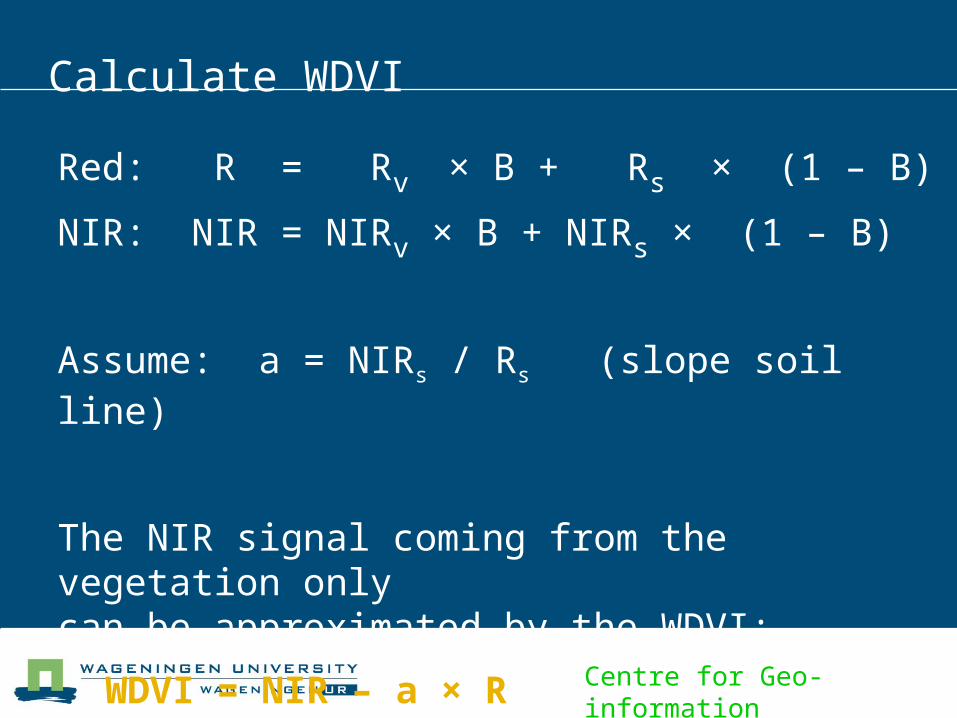
Calculate WDVI

Red: R = Rv × B + Rs × (1 – B)

NIR: NIR = NIRv × B + NIRs × (1 – B)

Assume: a = NIRs / Rs (slope soil line)

The NIR signal coming from the vegetation only

can be approximated by the WDVI:

WDVI = NIR – a × R


Hybrid Vegetation Indices

Soil Adjusted VI (SAVI): (1 + L) × (NIR – R)/(NIR +R + L)

L = l1 + l2 0.5

NIR

R

l1

l2

Broge & Leblanc, Remote Sens. Environ. 76 (2000): 156-172


Enhanced Vegetation Index (EVI)for use with MODIS data

C1 = atmospheric resistance red correction

coefficient [6.0]

C2 = atmospheric resistance blue correction

coefficient [7.5] L = canopy background brightness correction

factor [1.0]

http://tbrs.arizona.edu/project/MODIS/evi.php

LBCRCNIR

RNIREVI

21


Use of vegetation Indices

Estimation of: Leaf Area Index (LAI) Vegetation cover Absorbed Photosynthetically Active Radiation (APAR)

Chlorophyll or nitrogen content Canopy water content Biomass Carbon Structure of the canopy


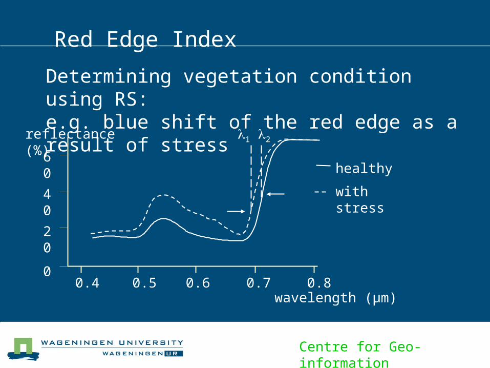
Red Edge Index

Determining vegetation condition using RS:e.g. blue shift of the red edge as a result of stress60

40

20

00.4 0.5 0.6 0.7 0.8

healthy

with stress

1 2

wavelength (µm)

reflectance (%)


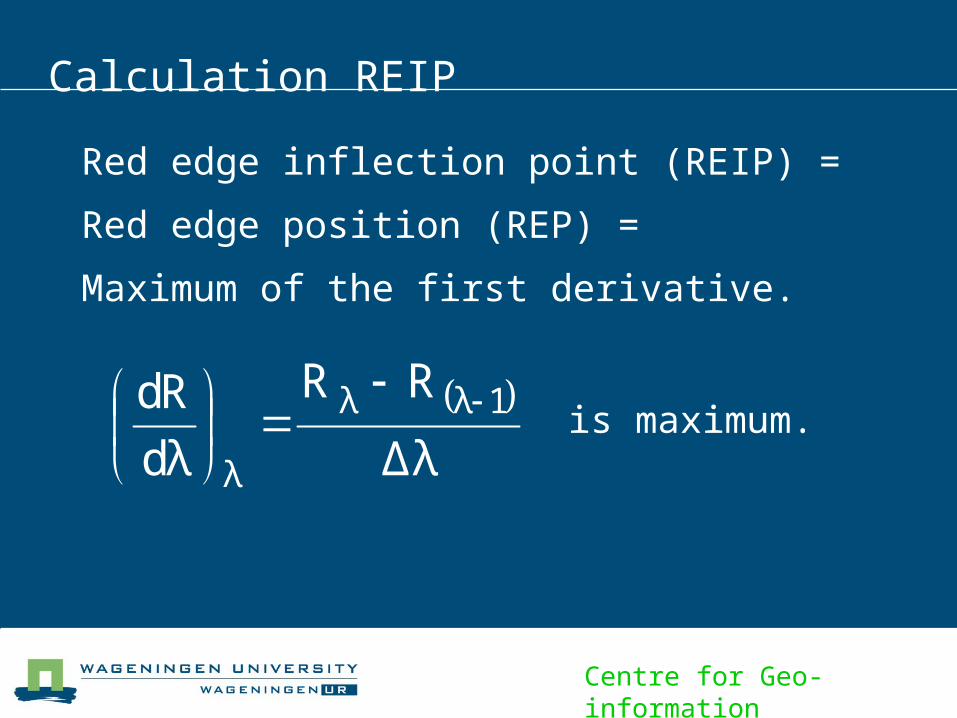
Calculation REIP

Δλ

RR

dλ

dR 1λλ

λ

Red edge inflection point (REIP) =

Red edge position (REP) =

Maximum of the first derivative.

is maximum.


680

690

700

710

720

730

740

0 10 20 30 40 50 60 70 80

Chlorophyll Content (mg.cm-2)

Re

d E

dg

e P

os

itio

n (

nm

)

LAI = 0.5

LAI = 1.0

LAI = 2.0

LAI = 4.0

LAI = 8.0

PROSPECT – SAIL simulation


690

700

710

720

730

740

0 5 10 15 20 25 30

Soil Reflectance (%)

Re

d E

dg

e P

os

itio

n (

nm

)

LAI = 0.5

LAI = 1.0

LAI = 2.0

LAI = 4.0

LAI = 8.0

Soil background influence


690

700

710

720

730

740

0 10 20 30 40 50 60 70 80 90 100

Visibility (km)

Re

d E

dg

e P

os

itio

n (

nm

)

CHL = 5

CHL = 10

CHL = 20

CHL = 40

CHL = 80

Atmospheric influence


Inverted Gaussian function

2

2o

oss 2σ

λλ exp RRRλR

σλREP o

Rs = shoulder reflectanceRo = minimum reflectanceo = wavelength at Ro

= Gaussian shape parameter


Linear interpolation method

0

10

20

30

40

50

60

600 650 700 750 800 850 900

Wavelength (nm)

Re

fle

cta

nc

e (

%)

Rre

lre


Linear interpolation method

700740

700780670

RR

R/2RR 40700REP


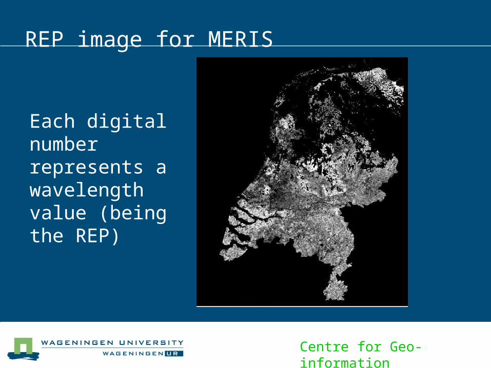
REP image for MERIS

Each digital number represents a wavelength value (being the REP)


Chlorophyll Index (CI)

CIred_edge = (RNIR / Rred_edge) – 1

= (R780 nm / R710 nm) – 1

As estimator of chlorophyll content

Gitelson et al., Geophysical Research Letters 33 (2006), 5 pp.

http://www.calmit.unl.edu/people/gitelson/


Photochemical Reflectance Index (PRI)

PRI = (R531 nm – R570 nm) / (R531 nm + R570 nm)

As estimator of photosynthetic activity

Gamon et al., Remote Sensing of Environment 41 (1992), 35 – 44.


Use of vegetation Indices

Estimation of: Leaf Area Index (LAI) Vegetation cover Absorbed Photosynthetically Active Radiation (APAR)

Chlorophyll or nitrogen content Canopy water content Biomass Carbon Structure of the canopy


Estimating Canopy Water Content (CWC)

970 nm 1200 nm

ASD Fieldspec Pro

0

0.1

0.2

0.3

0.4

0.5

0.6

0.7

400 600 800 1000 1200 1400 1600 1800 2000 2200 2400

Wavelength (nm)

Ref

lect

ance

970 nm 1200 nm


Reflectances Continuum removal: MBD, AUC, ANMB Water band indices: WI, NDWI

WI = R900/R970

NDWI = (R860 – R1240) / (R860 + R1240)

Derivatives

Estimators for Canopy Water Content


Results: PROSPECT-SAILH simulation CWC

y = -202.24x + 0.0437

R2 = 0.9849

0

5

10

15

20

25

30

35

40

-0.2 -0.15 -0.1 -0.05 0

Derivative @ 942.5 nm

Can

op

y w

ater

co

nte

nt

(to

n/h

a)


Results: Millingerwaard 2004 - FieldSpec

y = -155.2x + 4.0005

R2 = 0.7211

0

5

10

15

20

25

30

-0.15 -0.13 -0.11 -0.09 -0.07 -0.05 -0.03 -0.01

Derivative @ 936.5 nm

Can

op

y w

ater

co

nte

nt

(to

n/h

a)

0

2

4

6

8

10

12

Dry

wei

gh

t (t

on

/ha)


PROSPECT-SAILH

FieldSpec2004

HyMap2004

FieldSpec2005

AHS2005

DerivativeLeft slope

0.98@ 942.5 nm

0.72@ 936.5 nm

0.50@ 936 nm

0.55@ 936.5 nm

0.56@ 933 nm

DerivativeRight slope

[email protected] nm

[email protected] nm

0.45@ 1030 nm

[email protected] nm --

WI 0.94 0.37 0.38 0.40 0.41

NDWI 0.86 0.50 0.25 0.36 --

Summary


Continuum removal (1)

Use Continuum Removal to normalize reflectance spectra to allow comparison of individual absorption features from a common baseline. The continuum is a convex hull fit over the top of a spectrum utilizing straight line segments that connect local spectra maxima. The first and last spectral data values are on the hull and therefore the first and last bands in the output continuum-removed data file are equal to 1.0.

(Source: ENVI online help)

Convex hull

http://www.cse.unsw.edu.au/~lambert/java/3d/ConvexHull.html



http://speclab.cr.usgs.gov/PAPERS.refl-mrs/



MBD = Maximum Band Depth



AUC = Area Under CurveANMB = Area Normalized by the Maximum Band depth


Each endmember has a unique spectrum

IFOV of pixel

A

B

C

A

B

C

A single pixel with three materials A, B and C

Material Fraction

0.25

0.25

0.50

The mixed spectrum is just a weighted average

mix=0.25*A+0.25*B+0.5*C

Spectral unmixing aims at finding the fractions or abundances of end-members, which are spectrally pure by deconvolving them from a mixed spectrum

Reflectance spectra

Spectral unmixing


Mathematics of linear unmixing

Ri = reflectance of the mixed spectrum of a pixel

in image band i ¦j = fraction of end-member j

Reij = reflectance of the end-member spectrum j in band i

i = the residual error

n = number of end-members

Constraining assumptions: and

iij

n

jji fR

Re1

11

n

jjf 10 jf


Spectral unmixing at Cuprite

Alunite Calcite Kaolinite Silica Zeolite

RMSimage

Geologic mapfrom unmixing


Problems with unmixing

How to select the end members? Do these describe the data spectrally? Are these of interest? Is mixing a linear process?

Spectrometer

Incidentsolar irradiance

Heterogeneous IFOVfor a single pixel

Spectralunmixing


Spectral field measurements

Questions ?

© Wageningen UR

www.scopus.com/home.url

www.isiknowledge.com

http://www.scopus.com/home.url

http://www.isiknowledge.com/

vegetation indices and the red-edge index jan clevers centre for geo-information (cgi)

Documents