Vehicle Routing with Cross-Docking

Min Wen1, Jesper Larsen1, Jens Clausen1, Jean-François Cordeau2∗, Gilbert Laporte3

1Department of Informatics and Mathematical Modeling, Technical

University of Denmark, 2800 Kgs. Lyngby, Denmark2Canada Research Chair in Logistics and Transportation, HEC Montreal,

3000 chemin de la Cote-Sainte-Catherine, Montréal, Canada H3T 2A73Canada Research Chair in Distribution Management, HEC Montreal,

3000 chemin de la Cote-Sainte-Catherine, Montréal, Canada H3T 2A7

September 4, 2007

Abstract

Over the past decade, cross-docking has emerged as an important material handling tech-nology in transportation. A variation of the well-knownVehicle Routing Problem(VRP), theVehicle Routing Problem with Cross-Docking(VRPCD) arises in a number of logistics plan-ning contexts. This paper addresses the VRPCD, where a set of homogeneous vehicles areused to transport products from the suppliers to the corresponding customers via a cross-dock.The products can be consolidated at the cross-dock but cannot be stored for very long becausethe cross-dock does not have long-term inventory-holding capabilities. The objective of theVRPCD is to minimize the total traveled distance while respecting time window constraintsat the nodes and a time horizon for the whole transportation operation. In this paper, a mixedinteger programming formulation for the VRPCD is proposed. A tabu search heuristic is em-bedded within an adaptive memory procedure to solve the problem. The proposed algorithmis implemented and tested on data sets provided by the Danish consultancy Transvision, andinvolving up to 200 pairs of nodes. Experimental results show that this algorithm can pro-duce high quality solutions (less than 5% away from optimal solution values) within very shortcomputational time.

Keywords: Cross-docking, Vehicle Routing Problem, Pickup and Delivery.

∗Corresponding author (jean-francois.cordeau@hec.ca)

1

Introduction

Cross-docking is a relatively new warehousing strategy in logistics. It is defined as the consolida-tion of products from incoming shipments so that they can be easily sorted at a distribution centerfor outgoing shipments. The distribution center in this case is referred to as a cross-dock. It es-sentially eliminates the inventory holding function of a traditional warehouse while still allowingconsolidation. The shipments arriving from disparate sources are regrouped and dispatched di-rectly by the outgoing trailers without being stored. Shipments typically spend less than 24 hoursat the cross-dock, sometimes less than an hour. This way, cross-docking not only provides goodcustomer service but also yields substantial advantages over traditional warehousing: reduction ininventory investment, storage space, handling cost and order-cycle time, as well as faster inventoryturnover and accelerated cash flow (Cook, Gibson and MacCurdy, 2005; Apte and Viswanathan,2000).

Due to its remarkable benefits, cross-docking has been widely adopted in practice by manufac-turing and retailing companies. A successful application of cross-docking is found at Wal-Mart,the largest and highest profit retailer in the world. In the system used by this company, productsare continuously delivered to Wal-Mart’s cross-docks, where they are selected, repacked, and thendispatched to stores, often without ever sitting in inventory. By avoiding spending valuable timeand handling inventory cost, cross-docking has enabled Wal-Mart to adopt an everyday low pricestrategy and has helped the company improve its market share and profitability (Stalk, Evans andShulman, 1992). CompUSA is another major user of cross-docking: 70% of its products in dollarvolume goes through a cross-dock (Gentry, 2005).

Considerable research on cross-docking has been carried out in recent years. However, most ofthe papers have investigated the physical design of the cross-dock (Ratliff, Vate and Zhang, 1999;Bartholdi III and Gue, 2004) and its location (Gumus and Bookbinder, 2004). The very few papersthat deal with the transportation problems associated with cross-docking have studied two types ofnetwork models.

The first type of model is characterized by an "open" network, in which the distribution flow startsfrom a single supplier and ends at a single customer via a cross-dock without forming any loop.Work in this area includes Sung and Song (2003), Jayaraman and Ross (2003) and Chenet al.(2006). Sung and Song (2003) have discussed the problem of deciding whether to open a cross-dock or not, and the problem of assigning vehicles for transportation from a supplier to a singledestination via one of the open cross-docks. They have proposed a tabu search algorithm for thetransportation problem. Jayaraman and Ross (2003) have investigated a similar problem. Givena cost for opening each supplier, they have discussed how to decide whether a supplier should beopened or closed. Simulated annealing methods were used in their paper. In Chenet al. (2006),time windows for suppliers and customers are given, and the inventory cost at the cross-dock is alsotaken into consideration. These authors have proposed a hybrid metaheuristic combining simulated

2

annealing and tabu search.

In the second type of network model, each vehicle leaves the cross-dock to pick up or delivergoods and returns to the cross-dock after completing its tour. To the best of our knowledge, onlyone publication, that of Lee, Jung and Lee (2006), has studied a transportation problem of this type.This problem consists of a single cross-dock, multiple suppliers and multiple customers. The taskis to assign tours to a set of vehicles at the cross-dock so that suppliers and customers are visitedwithin their time windows. The authors assume that all vehicles should arrive simultaneously atthe cross-dock from their pickup routes. A mixed integer programming formulation and a tabusearch algorithm were proposed.

The problem considered in our study is theVehicle Routing Problem with Cross-Docking(VR-PCD). The problem is similar to that of Lee, Jung and Lee (2006) where the vehicles can pickup or deliver more than one supplier or customer, and the pickup and delivery routes start andend at the cross-dock. However, there is no constraint on simultaneous arrival for all the vehiclesin our problem. Instead, the dependency among the vehicles is determined by the consolidationdecisions. Moreover, each pickup and delivery has predetermined time windows.

The remainder of this paper is organized as follows. A detailed description of the VRPCD is givenin the next section. A mixed integer formulation of the problem is then presented, followed by aheuristic embedding tabu search within an adaptive memory procedure. The algorithm is imple-mented and tested on realistic data involving up to 200 supplier-customer pairs. Computationalresults are presented and conclusions follow.

Problem Definition

The VRPCD considered in this paper is in essence a problem of transporting products from aset of suppliers to their corresponding customers using a cross-docking strategy. Products fromthe suppliers are picked up by a fleet of homogeneous vehicles, consolidated at the cross-dock,and immediately delivered to customers by the same set of vehicles, without intermediate storage.Therefore, the problem involves not only vehicle route design, but also a consolidation decision atthe cross-dock.

A small VRPCD instance of five supplier-customer pairs (requests) is shown in Figure 1. The setof nodes {1, ..., 5} represents the suppliers and {1′, ..., 5′} represents the corresponding customers.Figure 2 illustrates the pickup and delivery routes for the three vehicles, all of which start and endtheir routes at the cross-dock. For example, the first vehicle makes pickups at nodes 1 and 2 anddelivers to nodes 1′, 2′ and 5′. Note that in the VRPCD, a supplier and its corresponding customerare not necessarily served by the same vehicle. For instance, request 5 is picked up by the thirdvehicle but delivered by the first vehicle. Hence, the third vehicle has to unload product 5 after itarrives at the cross-dock from its pickup route, and the first vehicle needs to load product 5 before

3

1

1'5'

3'

4'2'

3

5

4

2

Cross-dockterminal

Figure 1: A small instance of the VRPCD

it leaves for its delivery route. Figure 3 shows the details of the consolidation process taking placeat the cross-dock.

As in theVehicle Routing Problem with Time Windows(VRPTW), each node must be served byexactly one vehicle within its time window, the accumulated load of each route must not exceedthe vehicle capacity, and the time horizon for the whole transportation operation must be respected.At the cross-dock, for each vehicle the unloading must be completed before reloading starts. Eachvehicle can start unloading immediately after it arrives at the cross-dock from its pickup route.The duration of the unloading consists of a fixed time for preparation, and the time needed forunloading products, equal to the time for unloading each pallet multiplied by the number of pallets.For instance, suppose vehiclek reaches the cross-dock at 10:00. It needs to unload productsi1 andi2, whose demands are 5 and 9, respectively. Given that the fixed time for preparation is ten minutesand the time for unloading each pallet is one minute, the total unloading duration is 24 (= 10 + 5 +9) minutes. Note that the time at which vehiclek finishes unloading, i.e. 10:24, is also the time atwhich productsi1 andi2 are ready to be reloaded in their corresponding delivery vehicles.

1

1'5'

3'

4'2'

3

5

4

2

Vehicle 1

Vehicle 3Vehicle 2

Figure 2: Vehicle routes

4

1 2

3 4

5

1' 2' 5'

4'

3'

Reloading

Unloading

Unloading Reloading5

3

Vehicle 1

Vehicle 2

Vehicle 3

Figure 3: The consolidation process at the cross-dock

Mathematical formulation

We now present a mixed integer linear programming formulation for the VRPCD. Denote the setof pickup nodes byP = {1, ..., n} and the set of delivery nodes byD = {n + 1, ..., 2n}. Eachrequesti is identified by the node pair (i, i + n), wherei is the pickup node andi + n is theassociated delivery node. The cross-dock is represented by four nodes and denoted by the setO = {o1, o2, o3, o4}, where the first two nodes represent the starting and ending points for pickuproutes, and the last two for the delivery routes. Further, defineN = P ∪O∪D. The setE denotesall the feasible arcs in the network. It consists of the arcs{(i, j) : i, j ∈ P ∪ {o1, o2}, i 6= j} andthe arcs{(i, j) : i, j ∈ D ∪ {o3, o4}, i 6= j}. Let K be the set of vehicles.

The parameters are denoted as follows:

cij = the travel time between nodei and nodej ((i, j) ∈ E);

[ai, bi] = the time window for nodei (i ∈ N);

di = the amount of demand of requesti (i ∈ P );

Q = the vehicle capacity;

A = the fixed time for unloading and reloading at the cross-dock;

B = the time for unloading and reloading a pallet.

The variables are:

xkij =

{1 if vehiclek travels from nodei to nodej ((i, j) ∈ E, k ∈ K)0 otherwise;

uki =

{1 if vehiclek unloads requesti at the cross-dock(i ∈ P, k ∈ K)0 otherwise;

rki =

{1 if vehiclek reloads requesti at the cross-dock(i ∈ P, k ∈ K)0 otherwise;

5

gk =

{1 if vehiclek has to unload at the cross-dock(k ∈ K)0 otherwise;

hk =

{1 if vehiclek has to reload at the cross-dock(k ∈ K)0 otherwise;

ski = the time at which vehiclek leaves nodei (i ∈ N, k ∈ K);

tk = the time at which vehiclek finishes unloading at the cross-dock(k ∈ K);

wk = the time at which vehiclek starts reloading at the cross-dock(k ∈ K);

vi = the time at which requesti is unloaded by its pickup vehicle at the cross-dock(i ∈ P ).

In addition,M is an arbitrarily large constant.

The VRPCD can be formulated as follows:

minimize∑

(i,j)∈E

∑k∈K

cijxkij

subject to∑

j:(i,j)∈E

∑k∈K

xkij = 1 ∀i ∈ P ∪D (1)

∑i∈P

∑j:(i,j)∈E

dixkij ≤ Q ∀k ∈ K (2)

∑i∈D

∑j:(i,j)∈E

dixkij ≤ Q ∀k ∈ K (3)

∑j:(h,j)∈E

xkhj = 1 ∀h ∈ {o1, o3}, k ∈ K (4)

∑i:(i,h)∈E

xkih −

∑j:(h,j)∈E

xkhj = 0 ∀h ∈ P ∪D, k ∈ K (5)

∑j:(j,h)∈E

xkjh = 1 ∀h ∈ {o2, o4}, k ∈ K (6)

skj ≥ sk

i + cij −M(1− xkij) ∀(i, j) ∈ E, k ∈ K (7)

ai ≤ ski ≤ bi ∀i ∈ N, k ∈ K (8)

uki − rk

i =∑

j∈P∪{o2}xk

ij −∑

j∈D∪{o4}xk

i+n,j ∀i ∈ P, k ∈ K (9)

uki + rk

i ≤ 1 ∀i ∈ P, k ∈ K (10)1

M

∑i∈P

uki ≤ gk ≤

∑i∈P

uki ∀k ∈ K (11)

6

tk = sko2

+ Agk + B∑i∈P

diuki ∀k ∈ K (12)

wk ≥ tk ∀k ∈ K (13)

wk ≥ vi −M(1− rki ) ∀i ∈ P, k ∈ K (14)

vi ≥ tk −M(1− uki ) ∀i ∈ P, k ∈ K (15)

1

M

∑i∈P

rki ≤ hk ≤

∑i∈P

rki ∀k ∈ K (16)

sko3

= wk + Ahk + B∑i∈P

dirki ∀k ∈ K (17)

xkij , u

ki , r

ki , gk, hk ∈ {0, 1} ∀i ∈ P, (i, j) ∈ E, k ∈ K (18)

ski , tk, wk ≥ 0 ∀i ∈ N, k ∈ K (19)

vi ≥ 0 ∀i ∈ P. (20)

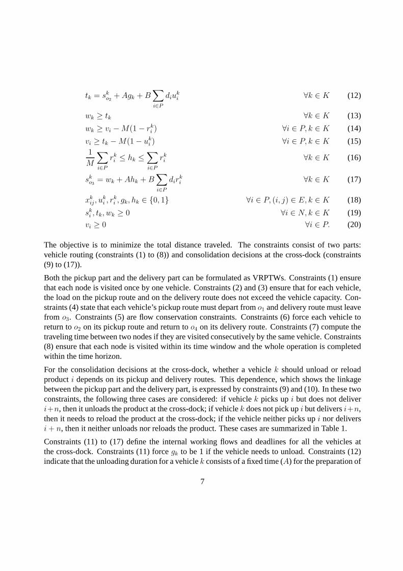
The objective is to minimize the total distance traveled. The constraints consist of two parts:vehicle routing (constraints (1) to (8)) and consolidation decisions at the cross-dock (constraints(9) to (17)).

Both the pickup part and the delivery part can be formulated as VRPTWs. Constraints (1) ensurethat each node is visited once by one vehicle. Constraints (2) and (3) ensure that for each vehicle,the load on the pickup route and on the delivery route does not exceed the vehicle capacity. Con-straints (4) state that each vehicle’s pickup route must depart fromo1 and delivery route must leavefrom o3. Constraints (5) are flow conservation constraints. Constraints (6) force each vehicle toreturn too2 on its pickup route and return too4 on its delivery route. Constraints (7) compute thetraveling time between two nodes if they are visited consecutively by the same vehicle. Constraints(8) ensure that each node is visited within its time window and the whole operation is completedwithin the time horizon.

For the consolidation decisions at the cross-dock, whether a vehiclek should unload or reloadproducti depends on its pickup and delivery routes. This dependence, which shows the linkagebetween the pickup part and the delivery part, is expressed by constraints (9) and (10). In these twoconstraints, the following three cases are considered: if vehiclek picks upi but does not deliveri+n, then it unloads the product at the cross-dock; if vehiclek does not pick upi but deliversi+n,then it needs to reload the product at the cross-dock; if the vehicle neither picks upi nor deliversi + n, then it neither unloads nor reloads the product. These cases are summarized in Table 1.

Constraints (11) to (17) define the internal working flows and deadlines for all the vehicles atthe cross-dock. Constraints (11) forcegk to be 1 if the vehicle needs to unload. Constraints (12)indicate that the unloading duration for a vehiclek consists of a fixed time (A) for the preparation of

7

k picks upi k deliversi + n k unloadsi k reloadsi∑j∈P∪{o2} xk

ij

∑j∈D∪{o4} xk

i+n,j uki rk

i

0 0 0 01 1 0 01 0 1 00 1 0 1

Table 1: Relationship betweenxkij anduk

i , rki

unloading, and the time for unloading the products, equal to the unit time for unloading a pallet (B)multiplied by the number of pallets (

∑i∈P diu

ki ) to be unloaded from the vehicle. Constraints (13)

and (14) ensure that a vehicle cannot start reloading until it finishes unloading, and all the productsto be reloaded on it are ready. The ready time of producti is represented by constraint (15), whichdepends on the time at which the pickup vehicle of producti finishes unloading. Constraints (16)and (17) for the reloading are similar to (11) and (12).

This formulation containsO(n2) binary variables,O(mn) continuous variable andO(n2m) con-straints. Without constraints (9) to (16), the model is essentially the problem of solving two in-dependent VRPTWs, abbreviated as 2-VRPTW. It is obvious that any optimal solution to this2-VRPTW provides a lower bound for the VRPCD. The difficulty in the VRPCD is that the pickupand delivery routes are not independent but correlated. This correlation results from the fact thatthe same vehicles need to first pick up and then deliver products within the time windows. There-fore, the search for an optimal solution is not only to find shortest routes for both operations, butalso to coordinate the exchanges of products at the cross-dock so that all time windows and thetime horizon are respected. These two aspects usually conflict with each other. The impact of thisconflict on the VRPCD solution will be illustrated in the computational experiments section.

Heuristics

Tabu search (TS) has proven to be one of the best available heuristic methods for solving VRPs,producing high quality solutions within a reasonable amount of computing time (Cordeauet al.,2002). The basic idea of TS is to locally and repeatedly modify a solution while memorizing themodifications to avoid cycling. Modifications to their attributes are stored in atabu listthat forbidstheir use for a certain number of iterations.

In this paper, we develop a TS algorithm for the VRPCD. Applying TS to a new problem re-quires taking the specific knowledge of the problem into consideration. In the VRPCD, due to theconsolidation at the cross-dock, computing the cost of even a simple insertion is very expensive.

8

To alleviate the computational burden, properties of insertions are investigated and new acceler-ating strategies are proposed, which have been proved to be very effective. Two neighbourhoodsare used alternately in the TS, which is finally embedded within an adaptive memory procedure(AMP). This enables the algorithm to reach good and robust solutions by repeating the TS fromdifferent good starting points.

The AMP is described next, followed by the proposed TS algorithm, and by a description of anefficient implementation of local search.

Adaptive memory procedure

In an AMP, a set of vehicle tours is stored in an adaptive memory (AM). A vehicle tour is definedas a pickup route and a delivery route operated by the same vehicle. An initial TS solution isconstructed by combining the selected vehicle tours, where the selection preference is probabilis-tically biased toward tours with good objective values. This idea was first proposed by Rochatand Taillard (1995) in the context of the VRP and of the VRPTW and has been proved to be veryeffective in providing high quality solutions for related problems.

In an AMP, an improved solution identified during the TS is considered. The vehicle tours in thissolution are labeled with the value of the objective function and are included in the AM. Concur-rently, the same number of tours with the highest label are removed from the AM. Consequently,the AM consists of a constant number of vehicle tours throughout the algorithm. Algorithm 1shows how to generate the initial TS solution from the AM. The probability assigned to a specificvehicle tour isP (r) = (max{lr|r ∈ AM)}− lr)/

∑r∈AM lr, wherelr is the label of therth vehicle

tour. A tour with a smaller value oflr will be selected with a higher probability. At each iterationone vehicle tour is selected and all incompatible tours are removed since each node can be servedby only one vehicle. The selecting procedure stops when there are no more vehicle tours compati-ble with those selected. Finally, the unvisited nodes are assigned to empty vehicles (see lines 8 to12).

Tabu search heuristic

Our TS algorithm is based on that of Cordeau, Laporte and Mercier (2001), in which infeasiblesolutions are allowed during the search. The cost function of a solutions is defined byf(s) =c(s) + αq(s) + βd(s) + γw(s), where

9

Algorithm 1 Generate initial solution from the memory1: AM ′ ← AM2: assign a probability to each element inAM ′

3: while AM ′ is not emptydo4: select a vehicle tourr from AM ′

5: delete the routes that cover a node covered by vehicle tourr6: end while7: let Nleft be the unserved nodes sorted in increasing order of radial angle8: while Nleft is not emptydo9: assign the nodes inNleft to an empty vehiclev′ one by one until the vehicle capacity is reached

10: remove fromNleft the nodes that are assigned tov′

11: end while

c(s) =∑k∈K

∑(i,j)∈E

cijxkij ; (21)

q(s) =∑k∈K

∑

i∈P

∑j∈P∪{02}

dixkij −Q

+

+

∑

i∈D

∑j∈D∪{04}

diykij −Q

+ ; (22)

d(s) =∑k∈K

(sk

o4− b0

); (23)

w(s) =∑k∈K

∑

i∈P

∑

j∈P∪{o2}sk

i xkij − bi

+

+∑i∈D

∑

j∈D∪{o4}sk

i xkij − bi

+ , (24)

where(x)+ = max{0, x}. In these equations,c(s) is the total distance traveled by all vehicles,q(s)is the total excess quantity in both the pickup and the delivery parts,d(s) andw(s) are the excessduration and total time window violations, respectively. Thus, ifs is feasible, thenf(s) = c(s).The coefficientsα, β andγ are positive self-adjusting penalties. At each iteration, the values ofα, β andγ are modified by a factor1 + δ > 1: if the current solution is feasible with respect toquantity (resp. duration, time windows), the value ofα (resp.β, γ) is divided by1 + δ; otherwise,it is multiplied by1 + δ.

In the TS, an insertion moves a nodei from its original vehiclek to another vehiclek′, as illustratedin Figure 4.

In some TS implementations (e.g., Barbarosoglu and Ozgur, 1999; Tang and Miller-Hooks, 2005),the solution improvement phase is divided into two stages: exploring a small number of moves(namely, small neighbourhood search), and exploring a large number of moves (namely, largeneighbourhood search). Empirical results show that alternating between small and large neigh-

10

i

kk'

i

kk'

Figure 4: Insertion move

bourhood search enables the search to evolve in an efficient way without degrading solution qual-ity.

In our TS algorithm, the same strategy is exploited. In the large neighbourhood search, everynode is moved to every position of every other vehicle. The complexity for this neighbourhoodis O(n2). In the small neighbourhood search, instead of searching the whole solution space, weselect a subset of nodesN ′ (N ′ ⊆ N) and move each of them to a specific subset of vehicles. Forinstance, a nodei′ (i′ ∈ N ′) is tentatively moved to each vehicle inM ′

i (M ′i ⊆ M). The ways

of selectingN ′ andM ′i are as follows: if in the current solution, a vehicle violates the capacity

constraint, exceeds the duration limit or involves any node not visited within its time window,all the nodes served by this vehicle will be added intoN ′ since the infeasibility of the solutionwill probably be reduced by removing a node from an infeasible route. After collecting all thenodes from all the infeasible vehicle routes, if the size ofN ′ is still less than a fixed numberµ,we randomly selectµ − |N ′| nodes and add them intoN ′ to make sure thatN ′ is not too small orempty when the solution is nearly feasible or feasible. When considering moving a nodei′ ∈ N ′

to vehicles inM ′i , we would likeM ′

i to be a set of vehicles that are very close to nodei′ in orderto minimize the total traveled distance. We sort all the nodesi ∈ N excepti′ in ascending orderof the distance betweeni andi′. The setM ′

i consists of all vehicles that cover any of theν nodesnearest toi′. Hence, each node inN ′ is moved to several of its nearest vehicle routes. With fixedvalues ofµ andν, the running time is independent of the size of the data.

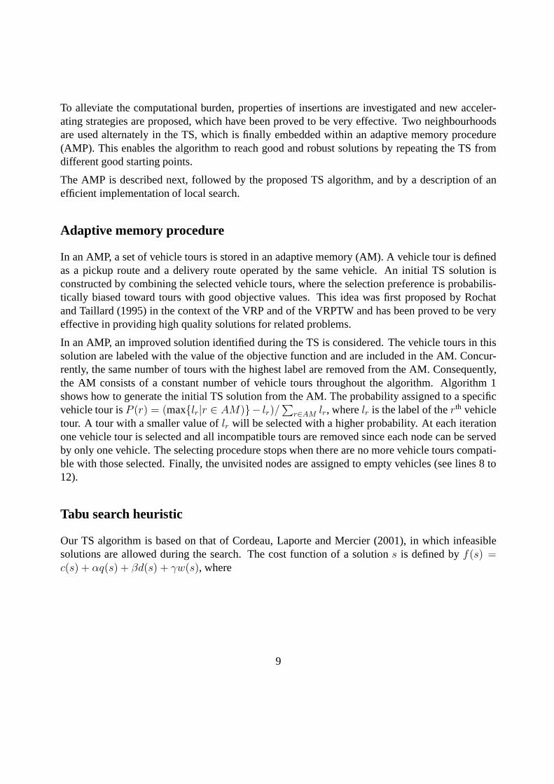
The strategy we used for switching between small and large neighbourhoods is the following: theTS starts with the small neighbourhood and switches to the large neighbourhood if there has beenno improvement in the best solution in the lastη iterations; when exploring the large neighbour-hood, if the best solution is updated withinσ iterations, the search process switches back to thesmall neighbourhood, otherwise the TS stops. The overall structure of TS is presented in Algorithm2.

As for short and long term memories, we use the same rules as in Cordeau, Laporte and Mercier(2001). To avoid cycling, if a node is removed from a vehicle, reinserting it in that vehicle isforbidden for the nextθ iterations unless the move satisfies anaspiration criterion, i.e. a feasible

11

Algorithm 2 Tabu search algorithm1: Stop = FALSE;Nb = 2; i = 0; s∗ = ∅; f(s∗) =∞2: while Stop == FALSEdo3: if Nb == 2 then4: Small neighbourhood search5: else6: Large neighbourhood search7: end if8: s = solution found by the neighbourhood search9: if f(s) < f(s∗) ands is feasiblethen

10: s∗ = s; i = 0; Nb = 211: else12: i++13: end if14: if Nb == 2 andi > η then15: Nb = 116: end if17: if Nb == 1 andi > σ then18: Stop = TRUE19: end if20: end while

solution better than the present best solution is found. To diversify the search, the move cost∆f isincreased by a penalty whose value is proportional to the frequency of the move. For more details,see Cordeau, Laporte and Mercier (2001).

Efficient implementation of local search

Compared with the VRPTW, an insertion move for the VRPCD is computationally much moreexpensive. Due to the consolidation at the cross-dock, the vehicles are no longer independent ofeach other. For example, an insertion move that shifts a supplieri from vehiclek to k′ will notonly affect the delivery route ofk andk′, but will also affect other related vehicles that serve thecorresponding customers of the suppliers served by vehiclesk andk′.

In order to accelerate the algorithm, we have studied the cost impact of a move. Denote the cur-rent solution byS1, the solution after the movei : k → k′ by S2, and the move cost by∆f .The change in total traveled distance is denoted as∆c. The changes in violation of quantity, dura-tion and time windows are denoted as∆q, ∆d and∆w, respectively. The following property holds:

Property If S1 is feasible, then∆f ≥ ∆c + α∆q.

12

Proof. Sincef(s) = c(s) + αq(s) + βd(s) + γw(s), the cost of a move can be represented as∆f = f(S2)−f(S1) = ∆c+α∆q +β∆d+γ∆w. SinceS1 is feasible, then∆d ≥ 0 and∆w ≥ 0hold. Hence,∆f ≥ ∆c + α∆q. �

Note that to calculateβ∆d andγ∆w, we need to exploit the complete information aboutS2 in-cluding the duration of each vehicle route and the visiting time of each node; on the other hand,∆c andα∆q can be very easily calculated without investigating the details inS2. Let ∆f ∗ denotethe minimum move cost among all moves considered. In the neighbourhood search of a currentlyfeasible solution, a move for which∆c + α∆q ≥ ∆f ∗ can be skipped to save computation time.We call this kind of skipping aconservative skip.

Preliminary tests have shown that very little computing time is saved by using theconservativeskipsince it only applies to feasible solutions. To reduce the computational time further, we havedeveloped anaggressive skipwhich applies when the route of vehiclek is feasible with respectto the duration and time window constraints. This skip is reasonable because removingi fromk is very likely to reduce the violation of routek, and insertingi into routek′ may increase theviolation of routek′. If vehiclek is already feasible,∆d and∆w are probably positive. The moveis therefore skipped if∆c + α∆q ≥ ∆f . Nevertheless, if routek is infeasible with respect to theduration and time window constraints, then the move should not be skipped.

Computational Experiments

Our TS heuristic was implemented in C and executed on a Linux computer with a 2.2GHz DualCore AMD Opterontm Processor 175 and 2 Gbytes of RAM. Due to the practical constraints, for adata set with 200 pairs of nodes, the users would expect to solve the problem relatively quickly. Asa result, the computational time of running the algorithm in this paper is limited to five minutes.

Data

The data used in this paper were generated from a real data set belonging to Transvision, a Danishlogistics consultancy based in Copenhagen. The real data are confidential and could not be pro-vided to us. The test data consist of five Euclidean sets, denoted by 200a, 200b, 200c, 200d and200e, respectively, where 200 stands for the number of supplier-customer pairs. Each set consistsof suppliers and customers with pickup and delivery locations (x, y) in meters. The time windowfor each node is two hours. The time horizon for the whole transportation operation is from 6:00 to22:00. The demand transported from each pickup location to the corresponding delivery locationis given in number of pallets. Vehicles drive at a constant speed of 60 km/h and have a capacity of33 pallets. It takes ten minutes to prepare a vehicle, plus an additional one minute for each pallet

13

to be loaded or unloaded. The locations of the suppliers, the customers and the cross-dock for onedata set are given in Figure 5. In this data set, the depot is located in Glostrup, near Copenhagen.The pickup points are mostly in Zealand where Glostrup is situated, and the delivery points aremostly in Jutland.

For preliminary testing purposes, small data sets with 20, 30, 50, 100 or 150 pairs of nodes weregenerated by randomly selecting the corresponding number of supplier-customer pairs. All the testdata can be accessed via the Internet at http://www2.imm.dtu.dk/∼mw/vrpcdData/.

Figure 5: Locations of pickup and delivery nodes for one instance of the VRPCD

Parameter tuning

The algorithm employs a set of parameters whose values require tuning before the algorithm isassessed. In Table 2, these parameters are listed and explained. Based on a large number of runs,the following set of parameters was finally selected: (δ, η, σ, ϕ, µ, ν) = (3, 1200, 800, 10n, n, 10),where then is the number of supplier-customer pairs.

In the AMP, it was found that the performance of the algorithm is not very sensitive to the AM sizeϕ. Preliminary results have shown thatϕ = 10n is large enough. The selection of the number ofAMP iterations is a tradeoff between performance and computational cost. Given the running timeof five minutes, three iterations are found to be suitable, which is in line with the setting used inTang and Miller-Hooks (2005).

14

δ: the maximum number of AMP iterations;η: the maximum number of non-improving iterations in small neighbourhood search in

TS;σ: the maximum number of non-improving iterations in large neighbourhood search in

TS;ϕ: the size of the AM;µ: the number of the selected nodes for the small neighbourhood;ν: in the small neighbourhood, a selected nodei is moved to the vehicles that cover the

ν nodes nearest toi;

Table 2: Parameters of the algorithm

As mentioned in the TS description, the alternate use of two neighbourhoods in the TS makes itpossible for the search process to move out of the current local optimum. This strategy has alreadybeen proved to be very effective in providing high quality solutions as stated in Tang and Miller-Hooks (2005). The same effect is achieved by our algorithm, as shown in Table 3. In the tests, thevalue ofν is 10 for the small neighbourhood andn for the large neighbourhood. Table 3 illustratesthe comparison between two-neighbourhood search and one-neighbourhood search. The first twocolumns are the data set descriptor and the number of supplier-customer pairs. Columns 3 and4 report the average solution value over 25 runs and the average computational time in secondsfor the two neighbourhood strategies adopted in our algorithm. Columns 5 and 6, and columns 7and 8 provide the corresponding results for the large neighbourhood search and the small neigh-bourhood search, respectively. According to Table 3, the two-neighbourhood strategy consistentlyoutperforms the other two one-neighbourhood strategies both in terms of average solution valueand computational time.

Two-neighbourhood Large neighbourhood Small neighbourhoodAverage Average Average Average Average Averagesolution time solution time solution time

Data set n value (seconds) value (seconds) value (seconds)

50a 50 6534.2 16 6568.1 27 6558.7 11100a 100 12982.9 63 13096.6 93 13265.9 20100b 100 14770.9 56 14864.9 92 14919.6 20150a 150 19871.3 139 19939.7 232 20304.5 38150b 150 21284.0 125 21374.3 218 21537.8 36200a 200 27684.8 274 27959.9 482 28107.7 73200b 200 27989.1 278 28241.2 517 28393.3 77

Table 3: Comparison of two-neighbourhood strategy and one-neighbourhood strategy

A large number of trials have shown that the selection ofη, σ andµ is not critical over a wide range.

15

The values 1200, 800 andn are selected based on the results and experience. The parametersα, β,γ are set as in Cordeau, Laporte and Mercier (2001).

Analysis of the main results of the algorithm

We now analyze the impact of the efficient implementation and the correlation among vehicles onthe behaviour of the algorithm, and we present results on the VRPCD instances.

Effect of the efficient implementation of the local search

The newaggressive skipdescribed in Section 4 is vital to efficiently narrow down neighbourhoodsize and to reach high quality solutions within short computing times. In theory, the ruling outprocess may cut off useful moves and degrade the solution quality slightly. However, it works verywell in practice.

A comparison between the results withaggressive skipand withoutaggressive skip(namely,fullsearch) is provided in Table 4. The column′Gap′ presents the percentage gap between the tworesults. It is calculated as100(zaggressive_skip − zfull_search)/zfull_search.

The column′Gap′ shows that the TS withaggressive skipperforms as well asfull search. The Gapis less than 0.3% for all the tests in Table 4. However, it can be seen, the computational time fortheaggressive skipis much shorter than for thefull search. Figure 6 shows the value of the bestsolution found as a function of the running time of the algorithm for data set 200a. As we cansee, theaggressive skipsignificantly speeds up the algorithm while maintaining almost the samesolution quality.

Aggressive skip Full searchAverage Average Average Averagesolution time solution time

Data Set n value (seconds) value (seconds) Gap (%)

100a 100 12981.9 63 12980.3 891 0.012100b 100 14770.9 56 14769.3 805 0.011100c 100 14145.1 57 14125.3 749 0.140150a 150 19871.3 139 19885.5 2790 -0.071150b 150 21284.0 125 21265.1 2565 0.089150c 150 20320.5 140 20326.7 2578 -0.031200a 200 27683.9 273 27676.2 6519 0.028200b 200 27989.1 278 27916.5 6449 0.260200c 200 26654.1 282 26640.3 6053 0.052

Table 4: Comparison of TS with and withoutaggressive skip

16

0 1000 2000 3000 4000 5000 60002.7

2.75

2.8

2.85

2.9

2.95

3

3.05

3.1

x 104

Figure 6: The effect ofaggressive skip. The short and long curves show the results with andwithoutaggressive skip, respectively

Impact of the correlation among vehicles on the VRPCD solution

To illustrate the impact of correlation among vehicles on the VRPCD solution, we vary the prepa-ration timeA and the timeB for reloading and unloading a pallet. AsA andB increase, it becomesmore time consuming to exchange products among vehicles at the cross-dock. Restricted by thetime windows at the delivery nodes, the algorithm will try to avoid unloading and reloading prod-ucts and thus hinder the optimization of distances traveled on both sides.

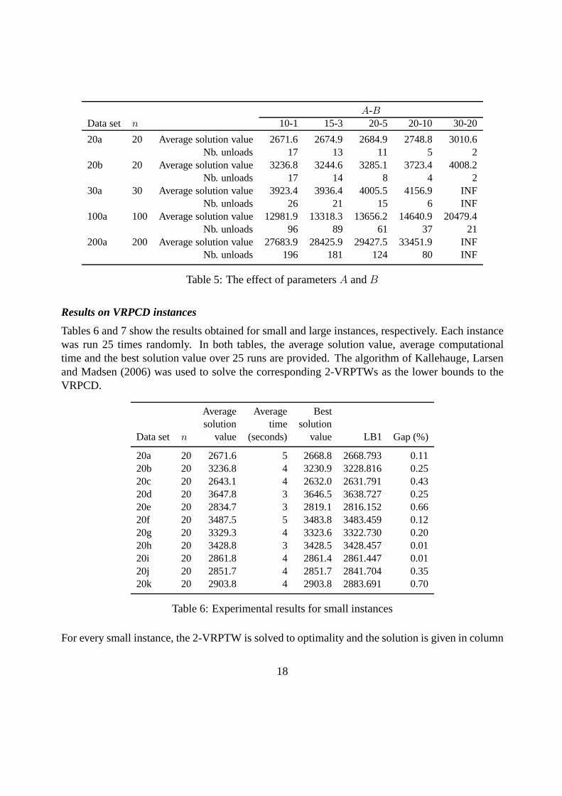
We have applied our algorithm with different settings ofA andB. The results are presented inTable 5. Five data sets (20a, 20b, 30a, 100a and 200a) were tested with different settings ofAandB. The settingA-B denotes the number of minutes required forA andB, respectively. Foreach data set andA-B setting, the average objective value over 20 random runs and the averagenumber of nodes whose products are unloaded at the cross-dock are given.′INF′ means no feasiblesolution was found in the 20 runs.

As expected, the best objective value the algorithm can find increases withA andB. For largeAandB, it is obvious that the optimal 2-VRPTW solutions do not yield good lower bounds for theVRPCD.

It should be stressed that other factors could affect the linkage of the pickup and delivery parts,such as the geographical distribution of suppliers and customers, the time windows, and the num-ber of supplier-customer pairs. When the distribution of suppliers is very different from that ofcustomers, for example when nearby suppliers have far away corresponding customers, when thetime windows are short, or when the number of suppliers and customers is large, the correlationbetween the two parts tends to be strong, i.e., the optimal solution of the VRPCD tends to be fartheraway from that of the 2-VRPTW.

17

A-BData set n 10-1 15-3 20-5 20-10 30-20

20a 20 Average solution value 2671.6 2674.9 2684.9 2748.8 3010.6Nb. unloads 17 13 11 5 2

20b 20 Average solution value 3236.8 3244.6 3285.1 3723.4 4008.2Nb. unloads 17 14 8 4 2

30a 30 Average solution value 3923.4 3936.4 4005.5 4156.9 INFNb. unloads 26 21 15 6 INF

100a 100 Average solution value 12981.9 13318.3 13656.2 14640.9 20479.4Nb. unloads 96 89 61 37 21

200a 200 Average solution value 27683.9 28425.9 29427.5 33451.9 INFNb. unloads 196 181 124 80 INF

Table 5: The effect of parametersA andB

Results on VRPCD instances

Tables 6 and 7 show the results obtained for small and large instances, respectively. Each instancewas run 25 times randomly. In both tables, the average solution value, average computationaltime and the best solution value over 25 runs are provided. The algorithm of Kallehauge, Larsenand Madsen (2006) was used to solve the corresponding 2-VRPTWs as the lower bounds to theVRPCD.

Average Average Bestsolution time solution

Data set n value (seconds) value LB1 Gap (%)

20a 20 2671.6 5 2668.8 2668.793 0.1120b 20 3236.8 4 3230.9 3228.816 0.2520c 20 2643.1 4 2632.0 2631.791 0.4320d 20 3647.8 3 3646.5 3638.727 0.2520e 20 2834.7 3 2819.1 2816.152 0.6620f 20 3487.5 5 3483.8 3483.459 0.1220g 20 3329.3 4 3323.6 3322.730 0.2020h 20 3428.8 3 3428.5 3428.457 0.0120i 20 2861.8 4 2861.4 2861.447 0.0120j 20 2851.7 4 2851.7 2841.704 0.3520k 20 2903.8 4 2903.8 2883.691 0.70

Table 6: Experimental results for small instances

For every small instance, the 2-VRPTW is solved to optimality and the solution is given in column

18

Results No limit test resultsAverage Average Best Average Best knownsolution time solution time solution Gap2

Data set n value (seconds) value (seconds) value LB2 (%)

30a 30 3923.4 9 3908.2 1787 3884.7 3757.04 4.0230b 30 4901.0 7 4855.6 1319 4824.1 4795.65 1.2530c 30 5146.8 7 5125.2 1495 5112.4 4968.30 3.1630d 30 3891.9 8 3865.0 1729 3850.0 3708.37 4.2230e 30 5084.4 7 5041.4 1468 5014.3 4913.24 2.6150a 50 6534.2 17 6497.3 3865 6471.9 6340.90 2.4750b 50 7504.9 19 7466.3 3185 7410.6 7201.89 3.6750c 50 7440.0 20 7350.5 3269 7330.6 7241.05 1.5150d 50 7107.6 20 7074.0 3658 7050.3 6887.93 2.7050e 50 7629.4 16 7571.5 3159 7516.8 7347.54 3.05100a 100 12981.9 63 12878.0 11543 12860.8 12555.57 2.57100b 100 14770.9 56 14646.8 9967 14526.1 14200.48 3.14100c 100 14145.0 57 14056.4 10677 13967.8 13631.24 3.12100d 100 13949.6 57 13844.4 11177 13763.3 13395.33 3.35100e 100 14396.1 63 14300.4 10643 14212.7 13745.60 4.04150a 150 19871.3 139 19784.0 24326 19537.3 19012.02 4.06150b 150 21284.0 125 21098.1 24461 20974.8 20371.08 3.57150c 150 20320.5 139 20166.2 23754 20126.5 19419.55 3.84150d 150 20891.3 123 20747.2 24468 20549.4 20013.37 3.67150e 150 20034.6 140 19888.5 23400 19848.5 19141.66 3.90200a 200 27683.9 273 27537.4 46586 27324.4 26538.53 3.76200b 200 27989.1 278 27851.7 43653 27637.7 26722.88 4.22200c 200 26654.1 282 26472.5 46389 26358.6 25607.31 3.38200d 200 28088.2 296 27935.3 46615 27749.7 26969.42 3.58200e 200 26868.6 275 26703.4 45649 26620.6 25776.01 3.60

Table 7: Experimental results for large instances

′LB1′ in Table 6. The gap between the′Average solution value′ and′LB1′ is given in column′Gap′

in Table 6. We can conclude that the algorithm can produce near optimal solutions (less than 1%away from the optimum) within very short computing times (less than 5 seconds) for all the smallinstances.

For the large instances, as 2-VRPTW itself is an NP-hard problem, it is very difficult to obtainthe optimal solution. Instead, we use a lower bound equal to the LP relaxation value computedat the root node of the 2-VRPTW, in column′LB2′ in Table 7. The gap between the′Averagesolution value′ and ′LB2′ is given in column′Gap2′ in Table 6. As can be seen from the table,

19

Gap2 is consistently below 5% for any data size in the tests. We consider this percentage to bevery satisfactory since it overestimates the true optimality gap. We also provide the best knownsolution values and the corresponding computational time in columns′No limit test results′ inTable 7. These results are obtained by removing the limit on the computational time and settingthe parameters as (δ, η, σ, ϕ, µ, ν) = (50, 15000, 15000, 10n, 2n, 10).

Conclusion

We have considered theVehicle Routing Problem with Cross-Dockingin which the goods fromthe suppliers and customers must be consolidated at a cross-dock terminal before being dispatchedto the customers. The problem was modeled and then solved by means of an efficient heuristicembedding tabu search within an adaptive memory procedure.

Since the cross-dock allows the transfer of goods between vehicles, the pickup and delivery ve-hicles are not independent of each other. The pickup and delivery parts are also correlated. As aresult of these interactions, calculating and performing a move can be difficult. A newaggressiveskip procedure introduced in the tabu search plays a key role in effectively narrowing down thenumber of moves to be calculated thoroughly and in reaching high quality solutions within shortcomputing times. The proposed algorithm was tested on realistic data sets involving up to 200pairs of nodes. Computational results show that it can provide high quality solutions (less than 5%away from the optimum) within very short running times.

Acknowledgements

This work was partially supported by the Canadian Natural Sciences and Engineering ResearchCouncil under grants 227837-04 and 39682-05. This support is gratefully acknowledged. Thanksare also due to Brian Kallehauge for computing the 2-VRPTW solutions, and to Jakob BirkedalNielsen from Transvision for providing the VRPCD data.

References

[1] Apte, U.M., Viswanathan, S., 2000. Effective Cross-Docking for Distribution Efficiencies,International Journal of Logistics: Research and Applications, 3, 291-302.

[2] Barbarosoglu, G., Ozgur, D., 1999. A tabu search algorithm for the vehicle routing problem,Computers & Operations Research, 26, 255-270.

20

[3] Bartholdi III, J.J., Gue, K.R., 2004. The best shape for a cross-dock,Transportation Science,38, 235-244.

[4] Chen, P., Guo, Y., Lim, A., Rodrigues, B., 2006. Multiple crossdocks with inventory and timewindows,Computers & Operations Research, 33, 43-63.

[5] Cook, R.L., Gibson B., MacCurdy, D., 2005. A lean approach to cross-docking,Supply ChainManagement, 9, 54-59.

[6] Cordeau, J.-F., Gendreau, M., Laporte, G., Potvin, J.-Y., Semet, F., 2002. A guide to vehiclerouting heuristics,Journal of the Operational Research Society, 53, 512-522.

[7] Cordeau, J.-F., Laporte, G., Mercier, A., 2001. A unified tabu Search heuristic for vehiclerouting problems with time windows,Journal of the Operational Research Society, 52, 928-936.

[8] Gentry, C.R., 2005. Million-Dollar,Chain Store Age, February, 54-56.

[9] Gumus, M., Bookbinder, J.H., 2004. Cross-docking and its implications in location-distribution system,Journal of Business Logistics, 25, 199-229.

[10] Jayaraman, V., Ross, A., 2003. A simulated annealing methodology to distribution networkdesign and management,European Journal of Operational Research, 144, 629-645.

[11] Kallehauge, B., Larsen, J., Madsen, O.B.G., 2006. Lagrangian duality applied to the vehiclerouting problem with time windows,Computers & Operations Research, 33, 1464-1487.

[12] Lee, Y.H., Jung, J.W., Lee, K.M., 2006. Vehicle routing scheduling for cross-docking in thesupply chain,Computers & Industrial Engineering, 51, 247-256.

[13] Ratliff, H.D., Vate, J.V., Zhang, M., 1999. Network design for load-driven dross-dockingsystems, Technical Report, The Logistics Institute, Georgia Institute of Technology, Atlanta.

[14] Rochat, Y., Taillard,E.D., 1995. Probabilistic diversification and intensification in localsearch for vehicle routing,Journal of Heuristics, 1, 147-167.

[15] Stalk, G., Evans P., Shulman L.E., 1992. Competing on capabilities: the new rules of corpo-rate strategy,Harvard Business Review, 70, 57-69.

[16] Sung, C.S., Song, S.H., 2003. Integrated service network design for a cross-docking supplychain network,Journal of the Operational Research Society, 54, 1283-1295.

[17] Tang, H., Miller-Hooks, E., 2005. A TABU search heuristic for the team orienteering prob-lem,Computers & Operations Research, 32, 1379-1407.

21