velocities and driving pressures of clay-rich sediments injected into clastic dykes...

Geophys. J. Int. (2008) 175, 1095–1107 doi: 10.1111/j.1365-246X.2008.03929.x

GJI

Sei

smol

ogy

Velocities and driving pressures of clay-rich sediments injected intoclastic dykes during earthquakes

Tsafrir Levi,1,2 Ram Weinberger,1 Yehuda Eyal,2 Vladimir Lyakhovsky1

and Eyal Heifetz3

1Geological Survey of Israel, 30 Malkhe Israel, Jerusalem 95501, Israel2Department of Geological and Environmental Sciences, Ben Gurion University of the Negev, Beer Sheva, Israel. E-mail: [email protected] of Geophysics and Planetary Sciences, Tel Aviv University, Tel Aviv 69978, Israel

Accepted 2008 July 27. Received 2008 June 22; in original form 2007 May 15

S U M M A R YWe studied the velocities and driving pressures associated with clastic-dyke formation in theAmi’az plain, where hundreds of clastic dykes cross-cut the soft rock of the late Pleistocenelacustrine Lisan Formation, within the seismically active Dead Sea basin. Flow of clasticmaterial into fractures and opening of the fractures are two mechanisms that occur duringearthquake-induced clastic dyke emplacement. Two analytic models were established, basedon field observations and experimental viscosity tests, to estimate the velocities and drivingpressures that were associated with dyke emplacement: (a) a channel flow for upward injectionof a clay–water mixture and (b) a profile of fracture dilation based on the elastic theory analysis.The two models predict that pressures between 1 and 10 MPa are generated in the source layerand dykes in the last stage of the injection process. In addition, the channel flow model predictsthat the injection velocity reaches metres to tens of metres per second and the emplacementtime of the clastic dykes is on a scale of seconds. It is suggested that the high pressurevalues represent the static stress drop during earthquake events or represent dynamic stressesresulting from the seismic waves which passed through the soft lacustrine rocks. In bothcases, the predicted high pressure values indicate that the clastic dyke was emplaced in closeproximity of an active segment of the Dead Sea Fault during the late Pleistocene-Holocene.

Key words: Fracture and flow; Palaeoseismology; Mechanics, theory, and modelling.

1 I N T RO D U C T I O N

Clastic dykes are discordant, tabular bodies comprised of weakly tostrongly lithified clastic detritus. They are formed either by passivedeposition of clastic material within pre-existing or earthquake-induced tensile fissures or by dynamic fracturing associated withinjection of clastic material during overpressure build-up. The lat-ter structures, known as injection clastic dykes, are the focus of thepresent study and are considered an example of natural hydraulicfractures (Jolly & Lonergan 2002). Hundreds of clastic dykes areexposed in Ami’az Plain, Dead Sea basin (Fig. 1). Previous studies(Levi et al. 2006a,b) demonstrated that part of these clastic dykes,connected to a clay-rich layer of the Lisan Formation (Fig. 1) wereformed by injection of material from that layer into the Lisan forma-tion. In such intrusions, the particle-water mixture, which is injectedunder high-pressure into the surrounding host rock, requires a sus-tained pressure difference between the mixture in the source layerand the mixture in the propagating fracture. This pressure differ-ence leads to dilation of the fracture and enables the particle-watermixture to flow through the fractures. Once the excess pressure de-creases, fracture propagation terminates and the injection processstops.

Emplacement of clastic dykes might form during strong earth-quakes (probably M ≥ 6.5). Earthquake-induced clastic dykes havebeen used for locating palaeo-epicentres (e.g. Galli 2000 and refer-ences therein). Calculating the injection velocities and the pressuresinvolved in the emplacement of clastic dyke may provide importantinformation about the stress values generated during earthquakes.

Engineering studies of ground deformation associated with earth-quakes have shown that near-surface granular porous material isliquefied by cyclic shear loading (Seed 1979; McCalpin 1996) orstatic stresses (e.g. Seed 1979) generated during earthquakes. Theliquefaction occurs as a consequence of the increased pore-waterpressure, whereby the granular porous material (i.e. sand) is trans-formed from a solid state into a fluid-like state. Soft sediment de-Formation is referred to as flowage or fluidization of cohessionlessclay-rich sediments during earthquakes (e.g. Mohindra & Bagati1996; Rodrıguez-Pascua et al. 2000; Moretti 2000). Behaviour ofsoft sediments under cyclic loading has been relatively less stud-ied compared with those of sands. Accordingly, the criteria used todefine the liquefaction of sand may no longer be applicable for clay-rich sediments (e.g. Yi lmaz et al. 2004 and references therein). Thefluidization process of the clay-rich source layer, several metres be-low the surface is associated with a pressure build-up that causes

C© 2008 The Authors 1095Journal compilation C© 2008 RAS

1096 T. Levi et al.

Figure 1. Location maps of the study area. The regional setting of theDead Sea Fault (inset) and the Ami’az Plain with the clastic dykes markedschematically by dashed lines. DSF, Dead Sea Fault; SD, Sedom Diapir(after Levi et al. 2006a).

the particle-water mixture to be injected upwards. The backgroundphysics of this pressure build-up process and its relation to the dy-namic stresses generated during earthquakes has been studied littleand not completely understood (e.g. Melosh 1996; Bachrach et al.2001).

In most cases, pressures and injection velocities that are gener-ated during earthquakes and form structures, such as clastic dykes,cannot be directly monitored. There are relatively few quantitativestudies of earthquake-induced structures (i.e. seismites), in generaland that of clastic dykes, in particular. The pressure values that are

estimated for dyke formation are generally of the order of severalMPa. This estimation is based on the assumption that the formationwas under lithostatic pressures corresponding to depths of tens tohundred of metres (e.g. Jolly & Lonergan 2002). Fluidized particle-water mixtures that have low viscosities are expected to flow underturbulence conditions (Turcotte & Schubert 1982).

In previous studies of clastic dykes in the Dead Sea basin Leviet al. (2006a,b) concluded that the dykes were emplaced duringearthquake events. Field observations and anisotropy of magneticsusceptibility (AMS) analysis suggest that the fluidization processof the source material was dynamic and occurred simultaneouslywith the fracturing process. The AMS fabric analysed by Levi et al.(2006a,b) indicates that the flow was turbulent and, qualitatively,associated with high injection velocities of well-mixed, homoge-neous fluid. The aim of this study is to quantify the velocity and theassociated driving pressures that are involved during the last stageof the injection process. We developed two mechanical models forthe emplacement of clastic dykes; one is based on the channel flowtheory and the other on the elastic crack theory. For this quantifi-cation, we also experimentally measured the dynamic viscosities ofthe clay-water mixture under different flow rates. The obtained in-jection velocities and driving pressures shed light on the fluidizationprocess and clastic dyke build-up during earthquakes.

2 G E O L O G I C S E T T I N G

The Ami’az Plain study area (Fig. 1) is located west of the MountSedom salt diapir (Zak 1967; Weinberger et al. 2006a,b), near thesouthwestern margin of the Dead Sea basin and adjacent to theDead Sea Fault, (e.g. Quennell 1959; Freund et al. 1968; Garfunkel1981). The Dead Sea basin is a continental depression, which isbounded on the east and west by a series of oblique–normal faults.The Ami’az Plain is one of the downfaulted blocks developed withinthe depression.

The incision of Nahal (Wadi) Perazim in the Ami’az Plain ex-poses the entire Lisan section and about 250 large-scale (height,lenght > 10 m) clastic dykes, which cut through the section. Basedon U–Th dating, the age of the Lisan Formation is between ∼70 000and 15 000 yr B.P. (Haase-Schramm et al. 2004). The bedrock of theAmi’az Plain is the ∼40 m thick Late Pleistocene lacustrine LisanFormation consisting mostly of authigenic (chalk) aragonite lami-nae, alternating with fine detritus layers (Begin et al. 1980). At thelower part of this formation, there are a few thick clay rich layers.Shaking and squeezing such wet clay layers causes a fast expulsionof pore water, a drastic loss of shear strength and consequent mate-rial flow and pressure build-up, which is not expected for the chalkyhost rock (Arkin & Michaeli 1986). The upper part of the LisanFormation consists of a ∼1 m thick relatively stiff gypsum layer.A thin veneer (<1 m) of aeolian and fluvial sediments overlies theLisan Formation and covers large parts of the plain.

The palaeoseismic record from the Dead Sea basin based on brec-cia layers reveals numerous moderate to strong earthquake eventsbetween 70 000 and 15 000 yr BP (e.g. Marco & Agnon 1995; Beginet al. 2005) and during the Holocene (Enzel et al. 2000; Ken-Toret al. 2001; Begin et al. 2005). The strongest recorded event in theDead Sea basin is the M = 6.2 earthquake of 1927 July 11; whose fo-cal mechanism solution is a left-lateral motion (Ben-Menahem et al.1976; Shapira et al. 1993). The strongest instrumentally recordedevent along the Dead Sea Fault is the Mw = 7.2 1995 November 22Gulf of Aqaba earthquake (Hofstetter 2003).

C© 2008 The Authors, GJI, 175, 1095–1107

Journal compilation C© 2008 RAS

Velocities and driving pressures of clay-rich sediments 1097

Most of the clastic dykes in the Ami’az Plain are injectionstructures, which were induced by late Pleistocene-Holocene earth-quakes along faults comprising the seismically active Dead SeaFault (Levi et al. 2006a,b). The earthquake induced fluidizationand injection of clastic material into dykes in the Ami’az Plainoccurred, based on resetting of quartz Optically Stimulated Lumi-nescence (OSL) signals, between 15 000 and 7 000 years BP (Poratet al. 2007).

The injection clastic dykes are composed of green clay, siltyquartz and some aragonite fragments. The dyke heights vary be-tween 5 mm and 18 m, the smallest of which (<0.5 m) are termeddykelets (Fig. 2b). The width (thickness) varies between 1 mm and0.18 m, and length, between 5 mm and 100 m. The width of thelarge-scale dykes (>10 m) is generally greater than 7 mm. In sev-eral cases, the measured width at the lower parts of these dykes issmaller than 7 mm, and it is not clear if such a narrow width is keptconstant along the entire height of the dykes.

A connection between a green clay-rich layer of the Lisan For-mation and the dyke-fill, observed in several dykes, unequivocallyindicates that the dykes were formed by injection of material from

Figure 2. (a) Large-scale clastic, dyke about 18 m high, crossing the Lisan section. The dyke shape resembles a filled channel. (b) Small-scale clastic dyke(dykelet) at the upper part of the Lisan section. The dykelet has a quasi-elliptical shape. (c) Two overlapping segments of dykelets at the upper part of the Lisansection. The Lisan laminae in the overlapping region are displaced. (d) Planar clastic dyke, filled with green clay sediment crosses the upper stiff gypsum layer.Dyke high is about 18 m. (e) Physical connection between a clastic dyke and the source layer (marked by black arrows) 18 m below the surface. Source layerthickness is ∼0.4 m.

that layer. Levi et al. (2006a,b) discussed several arguments stronglyindicating that the dykes, filled with the green clay-rich layer, arepressure-driven injected structures. The principal arguments arebriefly summarized below:

(1) There is a physical connection between the source layersand clastic-dykes indicating upward transport of sediments duringinjection.

(2) There is a similar mineral assemblage, based on the interpre-tation of XRD, and magnetic measurements of the rock, in both thesource layers and the respective dykes.

(3) The AMS analysis of the infill sediment shows a magneticinjection fabric compatible with injection flow and not with passivedeposition of clastic material into pre-existing fissures.

(4) The geometric pattern of small dykelets and segments formedin the upper part of the section shows that the lateral direction of thedyke propagation coincides with the lateral flow direction detectedby AMS analysis.

Dykes propagating below the source layer are terminated againstalternating gypsum and aragonite laminae of the lower Lisan

C© 2008 The Authors, GJI, 175, 1095–1107


1098 T. Levi et al.

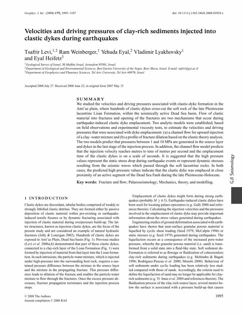
Figure 3. (a) Schematic representation of the two types of dykes: a blade-like dyke with a cross section resembling a channel and a branching dyke and itsassociated dykelets (left-hand panel). Some dykes/dykelets cross the upper stiff gypsum layer and some do not. (b) Model (A), showing upward flow along thex-axis under turbulent flow conditions. (c) Model (B), showing dilation profile of a representative dykelet.

Formation. Part of the upward propagating dykes commonly frac-ture and open the stiff gypsum layer (Fig. 3a), however, part occa-sionally terminate against this layer. Several injection dykes, whosewidth vary between ∼0.1 and 0.18 m, branch upward and split into3–5 large strands (Fig. 3a). Their pattern resembles the pattern ofdynamic fractures that bifurcate during upward propagation (e.g.Bahat et al. 2005). The large strands are typically segmented, form-ing numerous dykelets ∼13 m above the source layer. Assuming thatthe flow of clastic material followed the fracture propagation impliesthat the velocity of the fluid during dynamic fracturing could attainhigh values. The injection velocity could be even higher when thedykes reached the surface because at this stage, the pressure withinthe source layer is converted only to material flow. Overlapping ge-ometry between two adjacent segments implies opening of a frac-ture under internal pressure (Fig. 2c; e.g. Delaney & Pollard 1981;Gudmundsson 1995; Weinberger et al. 1995).

3 M E C H A N I C A L M O D E L L I N G O F T H EI N J E C T I O N DY K E S

3.1 Models for dyke emplacement

We present here two mechanical models that provide some estimatefor the source layer pressure and injection velocity of clay-water

mixture into the clastic dykes during their emplacement. Thesemodels are based on (1) channel flow analysis of planar dykes and (2)elastic crack theory analysis of dyke dilation profiles and the drivingpressure distribution in equilibrium state, which are achieved in thelast stage of the dyke propagation. The latter analysis is similar tothat of magmatic dyke dilation profiles (e.g. Pollard & Muller 1976;Delaney & Pollard 1981; Pollard 1987; Hoek 1994, 1995).

The assumptions for the models of dyke evolution and their jus-tification are based on our interpretation of field observations andAMS analysis (Levi et al. 2006a,b). The emplacement process ofthe dykes may be divided into three consequent stages:

(1) The pressure in the source layer increases to a level that ishigh enough for nucleation and growth of fractures. However, thedetails of the nucleation stage and the fluidization process of thesource layer are beyond the scope of the present study.

(2) Pressure-driven fractures (i.e. hydro-fractures) start to prop-agate upwards, downwards and laterally ahead of the injected clay–water mixture that consequently fills the fractures.

(3) The growth of fractures/dykes is mainly upward and later-ally because in many cases, they could not cross the stiff gypsumlayers that form mechanical boundaries below the source layer.In some cases, the fractures/dykes grew downwards and laterally,

C© 2008 The Authors, GJI, 175, 1095–1107



simultaneously with the injection of the clay-water mixture, untilthey were arrested and the process terminated (Fig. 3a). Levi et al.(2006a) demonstrate that expulsion of pore water after the emplace-ment of the dyke material was minor. Therefore, we assume that thepresent dyke dimensions should be similar to their dimensions justbefore the dykes were arrested. The final shape of the dykes mayclearly be seen in the dykelets that were emplaced close to thesurface, and represent the termination of the dynamic fracturingprocess (Figs 2b and 3a). Exposing these dykelets in 3-D, by grad-ual carving and removing the soft Lisan host rock, reveals a decrease(down to disappearance) in their dimensions in all directions. Thisindicates that the propagation velocity of these dykelets decreasedsignificantly and their growth can be approximated by quasi-staticconditions. Hence, a linear elastic analysis of the dykelet dilationprofiles provides a first-order approximation of their internal pres-sure (Fig. 3c). As to the large-scale dykes that propagated up tothe surface, channel flow conditions may have occurred at the timebefore the flow of material ceased.

3.2 Model (A): channel flow

3.2.1 Assumptions and justifications

Levi et al. (2006b) analysed the magnetic fabric of the clastic dykesand demonstrated that the AMS signals that evolved resulted fromfast flow conditions (>cm s−1). The AMS analysis also revealedthat although the flow direction was mainly upward, small eddieswere generated along the dykes width. This implies that at the finalstage of dyke emplacement the clay–water mixture filled the entiredyke width and the flow was fully turbulent.

In this section, we try to constrain the lower cut-off for the pres-sure gradient needed to assure a turbulent flow in a channel with adesignated width, using scaling relations for one-dimensional tur-bulent flow in a channel with a constant width. The present studydeals with fluid flow just before the injection ceased, implying thatthe channel flow process took place during a short time interval. Wealso assume that a mean steady-state flow was achieved.

3.2.2 Application to the clastic dykes

We apply scaling relations for 1-D turbulent channel flow (e.g.Turcotte & Schubert 1982). The model assumes an upward flowin the positive x-direction, which is driven by pressure gradient dp

dxresulting from two components, the difference between the sourcelayer pressure, pin at x = 0 and the pressure at the surface pout atx = 2l, and the buoyancy pressure gradient (Fig. 3b). Hence,

dp

dx= (pout − pin)

2l+ (ρf − ρr ) g, (1)

where 2l is the dyke height, ρ r is the host rock density, ρ f is thefluid density, g is the constant of gravitational acceleration, and pin

is the pressure at the source layer.For turbulent channel flow the pressure gradient is (Prandtl 1942)

dp

dx= − f

ρf u2

2w, (2)

where 2w is the width of the channel (dyke), u is the mean velocityand f is the friction factor.

The minus in eq. (2) stands for converting the negative sign ofthe pressure gradient to a positive value of the viscous resistanceand is related to the chosen coordinate system (Fig. 3b).

The friction factor is calculated as follows (Prandtl 1942)

f = 0.0791

Re0.25, (3)

where Re = 2wu/ν is the Reynolds number and ν is the kinematicviscosity. For a given Reynolds number the mean velocity in thechannel is

u = Reν

2w(4)

Combing eqs (1)–(4) enables expressing the pressure at the sourcelayer:

pin = 0.0791Re1.75ν2ρf l

4w3+ 2(ρf − ρE )gl + pout. (5)

The Reynolds number controls the transition from the laminar tothe turbulent flow. The onset of the turbulent flow in the channeloccurs at Re ≈ 2200 (e.g. Turcotte & Schubert 1982; Donald 1995).Substituting Re ≈ 2200 into eq. (4) and into eq. (5) enables the esti-mation of a velocity lower limit for the laminar–turbulent transitionand thus minimal pressure at the source layer.

pout depends on the conditions in the upper part of the dyke and isequal to the atmospheric pressure 0.1 MPa, if the dyke cuts the uppergypsum layer (Fig. 3a, Geologic Setting) and is open to the surface.This value is associated with the lowermost limit of the pressure inthe source layer. The lowermost limit of this pressure, correspondingto the onset of turbulence, increases proportionally to the clay-watermixture viscosity (∼ν2) and decreases proportionally to the channelwidth (∼w−3). This is because the derived formulation assumes thatthe source layer serves as an infinite reservoir with constant pressureand supplies mass flux into the channel according to its width andclay-water mixture viscosity.

During the dyke growth, the injection velocity could rise up tohigh values on the order of the fracture velocity. Notably, whenfractures made it up to the surface, the injection velocity could beeven higher than the fracture velocity (e.g. similar to super-sonicvelocities in volcano conduits e.g. Wilson et al. 1980). A highvalue of the pressure in the source layer is estimated, based on highvalues of the mean velocity uupper. Because emplacement of severaldykes is associated with dynamic fracturing (Levi et al. 2006a,b)it is likely that the velocity of the low-viscosity clay-water mixturecould attain the dynamic velocity of the dyke’s leading fractureudynamic. The dynamic velocity is about half of the Rayleigh wavevelocity uR, which is slightly below the shear wave velocity uS(e.g.Freund 1998):

uS =(

μ

ρr

)1/2

; u R ≈ 0.92us (6)

where μ is the shear modulus. Hence high value of the velocity is:

uupper ≤ udynamic ≈ 0.5

(μ

ρr

)1/2

(7)

This flow velocity is converted back to a high value for Re using eq.(4) and then to the source layer pressure Pin using eq. (5). Note thatthe high value of the flow velocity is only a comparable value tothe fracture dynamic velocity, and it is by no means an upper limitvalue or physically constrained parameter.

3.3 Model (B): crack elastic analysis of dyke dilationprofiles

3.3.1 Assumptions and justifications

The clastic dykes are filled fractures with smooth wall planes thatcross-cut the Lisan sediments in a brittle manner. Direct indications

C© 2008 The Authors, GJI, 175, 1095–1107


1100 T. Levi et al.

for brittle deformation during dyke emplacement include small-scale faulting and tilting of Lisan lamellae within an overlappingzone between two dyke segments (Fig. 2c). On the other hand, thereare no geometrical indications for ductile deformation and viscousfingering between the injected slurry and the Lisan host rock. OSLages of dyke emplacement suggest that many dykes intruded theLisan host rock after a significant drop in the Lisan water level(Porat et al. 2007). Hence, it is likely that the Lisan sediments lost asignificant amount of moisture during these thousands of years, andtheir properties were similar to those at present. Ductile deformationof the Lisan sediments prior to dyke emplacement is evidenced bytight synsedimentary folds in this formation. Therefore, we assumethat brittle fracturing was dominant during dyke emplacement, andhence, elastic theory can be applied to analyse their dilation profiles.

In this model, we assume that the opening profiles of the dykeletsare related to the existing pressure gradient, just before the injectionprocess ceased. The pressure gradient is related to the differencebetween the fluid pressure and the ambient stress in the host rock.The pressure gradient is comparable to the fluid pressure in the as-sociated dykelet because the lithostatic pressure in the upper sectionof the Lisan host rock is negligible. In addition, because the dykeletswere formed in the upper section and were physically connected tothe source layer via the large-scale dykes, their pressure gradientscan estimate the pressure in the source layer.

3.3.2 Application to the clastic dykes

This section presents the analysis of the measured dilation profiles2w(x) and estimated driving pressure distributions �p(x) for theclastic dykes. Following previous studies (Pollard 1976; Pollard &Muller 1976; Delaney & Pollard 1981; Hoek 1995), driving pressuredistributions are approximated by a sum of three linear normal-stressgradients that act on the fracture walls:

�p(x) = �p0 + (∇ pa + ∇ ps)(x − l) for (0 = x = l), (8a)

�p(x) = �p0 + (∇ pa − ∇ ps)(x − l) for (l < x = 2l) (8b)

where l is the half dyke height, x goes from 0 to 2l (Fig. 3c),�p0 is the uniform normal stress, ∇ pa is the asymmetric linearstress gradient and ∇ ps is the symmetric linear stress gradient. Thegeneral dilation profile solution is (Delaney & Pollard 1981):

2w(x) = �p0

M

[2√

2xl − x2]

+ ∇ pa

M

[(x − l)

√2xl − x2

]

+∇ ps

M

2

π

[l√

2xl − x2 + (l − x)2 ln

∣∣∣∣ (l − x)

l − √2xl − x2

∣∣∣∣]

,

(9)

where M is expressed through the shear modulus μ and Poisson’sratio ν elastic:

M = μ

(1 − ν). (10)

The dilation profile of the dyke is composed of three parts(eq. 9, from left- to right-hand side): (1) the elliptical shape; (2)the teardrop shape and (3) the diamond-shape. The combination ofthe three dilation profiles results in four models of driving pressuredistribution that are analysed by the best-fit method (least squares):

(I) �p0 = 0, ∇ pa = 0, ∇ ps = 0;(II) �p0 = 0, ∇ pa = 0, ∇ ps = 0;(III) �p0 = 0, ∇ pa = 0, ∇ ps = 0;(IV) �p0 = 0, ∇ pa = 0, ∇ ps = 0.

4 RO C K A N D F LU I D P RO P E RT I E S

The mechanical properties of the Lisan sediments were seldommeasured due to their weakness and fragility. Hence, we use pub-lished data on soft sediments including that obtained on the latePleistocene lacustrine Samra Formation (Chetrit 2004), which sed-imentologically is similar to the Lisan Formation. Soft sedimentspossess higher Poisson’s ratios than hard rocks (Othman 2005).Therefore, we used 0.4 for the Poisson’s ratio, which is also inagreement with the suggested 0.3–0.5 values of clay-rich sediments(e.g. Gee-Clough et al. 1994; Vallejo & Lobo-Guerrero 2002;Chetrit 2004; Othman 2005; Bala et al. 2006). For the dykeletsdeveloped close to the surface, we used a range of shear moduliibetween 50 to 100 MPa (e.g. Bala et al. 2006). For the entire Lisansection, we set a shear modulus equal to 100 MPa, which is inagreement with other experiments of soft sediments (e.g. Gannonet al. 1999; Schneider et al. 1999; Chetrit 2004; Yuan-qiang & Xu2004; Bala et al. 2006). The rock density for the whole Lisan sec-tion was set to 1400 kg m−3, and the maximum tensile strength isabout T o = 0.1 MPa (Arkin & Michaeli 1986). These values wereapplied to the analyses of dyke dilation profiles. There is no directinformation about the water quantity during the injection process.Reasonable viscosity values can be suggested based on the geologicsetting of the dykes and viscosity experimental tests carried out inthe present study. For the channel flow analysis we used two valuesof kinematic viscosity, ν = 0.3E – 04 m2 s−1 and 1.5E – 04 m2 s−1

(Appendix), where the Lisan clay-water mixture density is1700 kg m−3 and 1950 kg m−3, respectively.

5 R E S U LT S

5.1 Model (A)

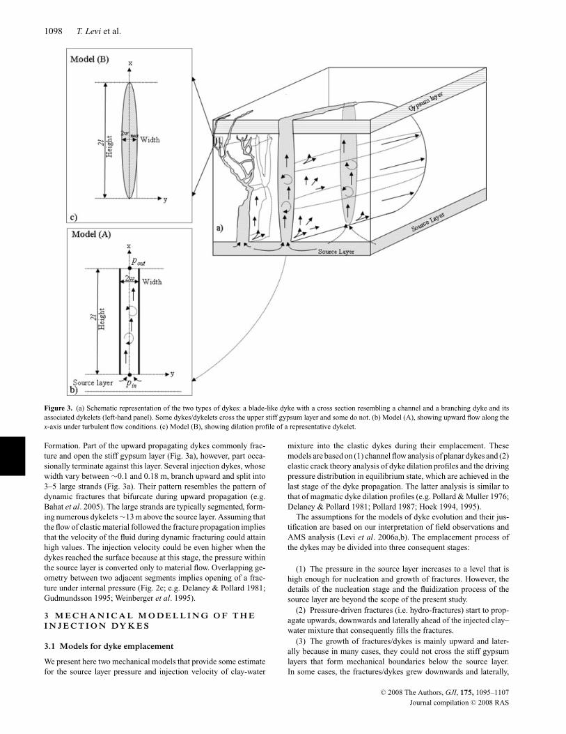
The model starts by calculating the maximum injection velocityusing eq. (4). Eighteen runs were preformed for nine channel widths(0.05, 0.07, 0.09, 0.1, 0.12, 0.14, 0.16, 0.18 and 0.2 m) and twokinematic viscosities (0.3E – 04 and 1.5E – 04 m s−1). The upperRe was set for each dyke width according to the upper velocitycalculated by eq. (7).

The calculated injection velocities vary from 0.2 to ∼ 250 m s−1

and the corresponding values of Re vary between 2.2 × 103 and∼1 × 106 (Fig. 4). The lowest value of the injection velocity wasobtained for a kinematic viscosity of 0.3E – 04 m2 s−1, dyke widthof 0.2 m and Re = 2.2 × 103 (Fig. 4, run i1). Higher values wereobtained in every run by increasing the Reynolds number (Fig. 4).Based on the upper Re values obtained for each run in Fig. 4 (42 ×103 ≤ Re ≤ 90 × 104), the pressure at the source layer calculated byeq. (5) varies between ∼0.2 and ∼65 MPa. The lowest and highestpressure values obtained are for run i1 and run a2, respectively(Fig. 5).

Variations in the dyke widths (thicknesses) resulted in significantvelocity changes of tens of metres per second and pressure changesof several MPa (e.g. run d2 and run a2 in Figs. 4 and 5). Variations ofthe dynamic viscosity also resulted in significant velocity changeson the order of tens of metres per second and pressure changes ofseveral MPa (e.g. run a1 and run a2 in Figs. 4 and 5).

5.2 Model (B)

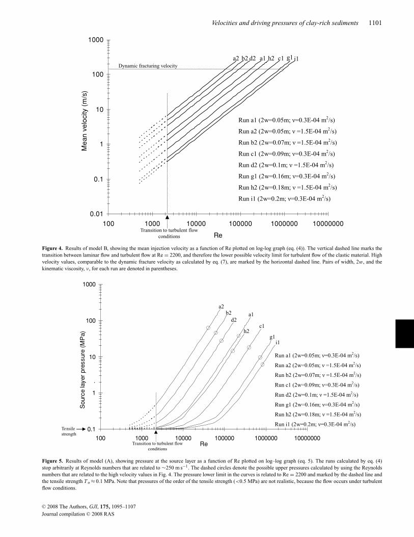
The geometric analysis of five dykelets is presented in Figs 6(a) and(b). The driving pressure distributions are calculated by analyzingthe coefficients of eq. (9) and using eqs 8(a) and (b) (Figs 7a and b).

C© 2008 The Authors, GJI, 175, 1095–1107



Run a1 (2w=0.05m; =0.3E-04 m2/s)

Run a2 (2w=0.05m; =1.5E-04 m2/s)

Run b2 (2w=0.07m; =1.5E-04 m2/s)

Run c1 (2w=0.09m; =0.3E-04 m2/s)

Run d2 (2w=0.1m; =1.5E-04 m2/s)

Run g1 (2w=0.16m; =0.3E-04 m2/s)

Run h2 (2w=0.18m; =1.5E-04 m2/s)

Run i1 (2w=0.2m; =0.3E-04 m2/s)

0.01

0.1

1

10

100

1000

100 1000 10000 100000 1000000 10000000

Re

Mea

n ve

loci

ty (

m/s

)

a2 b2 d2 h2 a1 c1 g1 i1 Dynamic fracturing velocity

Transition to turbulent flow conditions

Figure 4. Results of model B, showing the mean injection velocity as a function of Re plotted on log-log graph (eq. (4)). The vertical dashed line marks thetransition between laminar flow and turbulent flow at Re = 2200, and therefore the lower possible velocity limit for turbulent flow of the clastic material. Highvelocity values, comparable to the dynamic fracture velocity as calculated by eq. (7), are marked by the horizontal dashed line. Pairs of width, 2w, and thekinematic viscosity, ν, for each run are denoted in parentheses.

.

i1

Tensile strength

0.1

1

10

100

1000

100 1000 10000 100000 1000000 10000000Re

Sou

rce

laye

r pr

essu

re (

MP

a)

a2b2

h2

a1

c1

g1

d2

Transition to turbulent flow conditions

Run a1 (2w=0.05m; =0.3E-04 m2/s)

Run a2 (2w=0.05m; =1.5E-04 m2/s)

Run b2 (2w=0.07m; =1.5E-04 m2/s)

Run c1 (2w=0.09m; =0.3E-04 m2/s)

Run d2 (2w=0.1m; =1.5E-04 m2/s)

Run g1 (2w=0.16m; =0.3E-04 m2/s)

Run h2 (2w=0.18m; =1.5E-04 m2/s)

Run i1 (2w=0.2m; =0.3E-04 m2/s)

Figure 5. Results of model (A), showing pressure at the source layer as a function of Re plotted on log–log graph (eq. 5). The runs calculated by eq. (4)stop arbitrarily at Reynolds numbers that are related to ∼250 m s−1. The dashed circles denote the possible upper pressures calculated by using the Reynoldsnumbers that are related to the high velocity values in Fig. 4. The pressure lower limit in the curves is related to Re = 2200 and marked by the dashed line andthe tensile strength T o ≈ 0.1 MPa. Note that pressures of the order of the tensile strength (<0.5 MPa) are not realistic, because the flow occurs under turbulentflow conditions.

C© 2008 The Authors, GJI, 175, 1095–1107


1102 T. Levi et al.

Model I

b1)

-5 -5

0 0.1 0.2 0.3 0.4 0.50

0.004

0.008

0.012

Model II

0 0.1 0.2 0.3 0.4 0.50

0.005

0.01

0.015

Height m)

Model I

0 0.1 0.2 0.3 0.4 0.50

1

2

3

Height (m)0 0.1 0.2 0.3 0.4 0.5

0

0.4

0.8

1.2

1.6

Height (m)

Height (m)

a1)

a2) b2)

Dila

tion

(m)

Dila

tion

(m)

Sr Sr

Figure 6. Results of model (B), showing the measured (dashed line) and the modeled (solid line) dilation profile (eq. 9) of two representative clastic dykes(a1, b1; fracture 1 and fracture 2 in Table 1) and their sum of errors (a2, b2). The appropriate model is marked on the profile.

High R2 values for the four models I–IV imply that the elas-tic openings of the dykelets fit well with the linear elastic theory.Model II and model IV generally have higher r-squared values(Table 1). The average driving pressures for both G = 50 and 100MPa calculated by model IV is ∼4 MPa (Fig. 7).

6 D I S C U S S I O N

During strong earthquakes, tensile stresses are induced at the sur-face, forming tensile fractures at the Earth’s surface (e.g. Dalgueret al. 2002). Such fissures could be passively filled with clasticsediment from above (e.g. Eyal 1988), forming so-called Neptu-nian dykes. Field observations strengthened by magnetic AMS flowanalysis demonstrated that the clastic dykes presented in the Ami’azPlain, Lisan Formation, Dead Sea basin, were formed due to the in-jection of clay-water mixture (Levi et al. 2006a,b). Therefore, wesuggest that the values of the driving pressures discussed belowrepresent the internal pressure in the source layer.

6.1 Driving pressures and injection velocities

The two models presented in this study provide a tool for estimatingthe injection velocities and driving pressures during the clastic dykesemplacement. To get reliable results, we used a range of rock andfluid properties, which are based on our laboratory measurements of

viscosity (Appendix) and on published data of clay-rich sediments.The injection through the dyke-channel (Model A) is considered,based on the measured viscosities, to be Newtonian–Poiseuille flow.This allows us to provide a first order approximation of the dykeflow velocities and pressures during earthquake events. Numericalsimulations of non-Newtonian flow within the dykes are beyondthe scope of the present study and will be presented in a follow-uppaper.

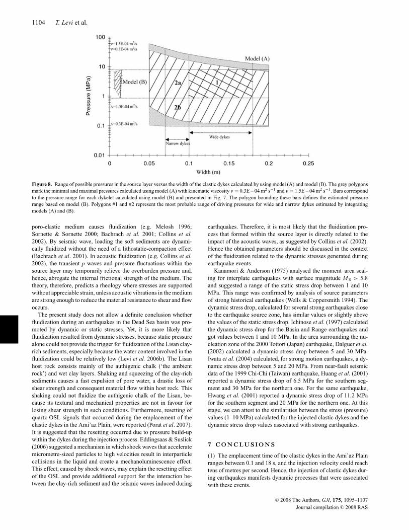
The estimation of the lower limit for the driving pressure andinjection velocity is based on scaling relations for 1-D turbulentflow in a channel with a constant width. This approach (Model A)estimates the minimal driving pressure (Fig. 8) needed to assure aturbulent flow in a channel of a designated width. The lower greypolygon marks the range of minimal driving pressures, calculatedby using the lowest value (ν = 0.3E-04 m2 s−1) and the highest value(ν = 1.5E – 04 m2 s−1) of the laboratory-measured kinematic vis-cosity. Fig. 7 demonstrates the distribution of driving pressure cal-culated with model (B) for every dykelet. Bars shown in Fig. 8correspond to the maximal and minimal values of these pressuredistributions and define the polygon bounding the estimated pres-sure range based on model (B). The dykelets analysed here re-sulted from dynamic branching of the relatively wide dykes (0.1–0.18 m). Hence, the obtained pressure range of model (B) couldbe viewed as a lower limit for the driving pressure for this groupof dykes. The most probable range of driving pressures for widedykes falls within 1–25 MPa, where the lower limit of the pressure

C© 2008 The Authors, GJI, 175, 1095–1107



0

0.5

1

1.5

2

0 2 4 6 8Pressure (MPa)

Hei

ght (

l)

54

213

6

Figure 7. Pressure distribution (eqs 8a and b) marked by solid line alongrepresentative dykelets using model IV and G = 100 MPa. Numbers arerelated to fracture number in Table 1. The range of the pressure values arelimited by fracture 2 and fracture 6.

Table 1. Output of Model B.

Number Fracture type R2 per mode typeI II III IV

1 Fracture 1-single fracture 0.87 0.90 0.88 0.902 Fracture 2-single fracture 0.99 0.99 1.00 1.003 Fracture 3-single fracture 0.91 0.94 0.91 0.944 Fracture 4-segment a 0.85 0.90 0.86 0.915 Fracture 4-segment b 0.81 0.95 0.81 0.956 Fracture 4-segment a & segment b 0.74 0.93 0.74 0.93

is based on model (B) and the high value on model (A). Finally, theoverlapping driving pressures of the two models are between 1 and10 MPa (Polygon #1, Fig. 8). Because the two different models givean overlapping range of driving pressures, it is most probably thatthis range of driving pressures existed within the source layer. Itis most likely that wider dykes, associated with large elastic defor-mations, were emplaced under higher driving pressures, probablygenerated by stronger seismic events or due to more efficient localpressure build-up in the source layer. We note that the higher valuesof driving pressures in polygon #1 fall very close to the drivingpressures obtained for dynamic fracture velocity (Fig. 8, upper greystrip), and therefore, dynamic branching of the wider dykes is veryreasonable.

Scaling relations for 1-D turbulent flow in a channel also enablesto estimate the injection velocities. Based on the lower value of thedriving pressure (1 MPa), we derived the associated Re numbers

from Fig. 5 and, consequently, substituted them in Fig. 4 to obtaina lower value for the injection velocity of ∼10 m/s. For a range ofinjection velocities between 10 and 130 m s−1 (i.e. dynamic frac-ture velocity), the duration of dyke emplacement is ∼0.1–2 s for a18-m-high dyke.

Branching or small dykelets connected to the main channel werenever observed in association with relatively narrow dykes (<0.1m). Therefore, we speculate that the narrow dykes were emplacedunder driving pressures equal (polygon #2a) or lower (polygon #2b)than the pressures of the polygon #1. Even if the narrow dykeswere emplaced during the same seismic event and were driven bythe same pressure, their injection velocity is expected to be lowerthan that of the wide dykes and fall below the threshold of dynamicbranching. These dykes could also be formed due to a lower drivingpressures, marked by the polygon #2b. Still, the injection velocityof the narrow dykes is estimated to be 1 m s−1 corresponding to theduration of the dyke emplacement 18 s.

The above velocities are comparable to velocities obtained dur-ing a hydro-abrasive erosion process in brittle materials in whichmaterial is removed by high speed of water jet mixed with solid par-ticles. The velocity of a water jet that succeeded in penetrating softrocks varied from 92 to 200 m s−1 and was associated with pressurebetween 5 and 22 MPa (Momber 2004). The predicted velocity forsand liquefaction is about 2 m s−1 (Gallo & Woods 2004), which iswithin the lower range of velocities that were obtained in the presentstudy for clastics injected into dykes.

For flow of sand-water mixtures in 10–100 m height vertical con-duits, Gallo & Woods (2004) calculated overpressures between 0.35to 1 MPa. In their model, the overpressures are formed due to thedifference between the densities of the host rock and the sand-watermixture. Pressure gradients results from the difference between theoverpressures and the frictional resistance, similar to the evolvedpressure gradients in the present model (see eq. 5). The modelsof this study calculate the velocities needed to obtain a turbulentflow, and based on these velocities, determine the pressures thatare also consistent with that needed to dilate the fractures. The ob-tained pressures for the present geological setting and mechanicalapproach are about one order of magnitude higher than those ofGallo & Woods (2004).

Jolly & Lonergan (2002) calculated an overpressure of severalMPa for a sandy source layer at hundreds of metres below thesurface. In their model, similar to that of Gallo & Woods (2004), theoverpressure is built-up by the difference between the host rock andthe sand-water mixture densities. However, the injection velocities,as well as the dyke dilation, were not considered. Their calculationscannot be directly applied to clastic dykes at shallow depth, such asthose in the Lisan Formation, because the differences between theLisan host rock and the clay-water mixture densities are insufficientto drive a turbulent flow. The pressure-driven mechanism of theclastic dykes emplacement is compatible with field observations,demonstrating that in the same injection system the flow can beupward, horizontal and even downward (Levi et al. 2006b).

6.2 Pressures during earthquakes

The response of materials to a sudden applied stress is still notwell understood (e.g. Sawicki & Mierczynski 2006), especiallyfor clay-rich sediments (Yılmaz et al. 2004). So far, only a fewstudies have dealt with the fluidization mechanism of soft sed-iments during earthquake loading. Most of them suggest thatthe direct impact of the p-wave loading that passed through the

C© 2008 The Authors, GJI, 175, 1095–1107


1104 T. Levi et al.

Figure 8. Range of possible pressures in the source layer versus the width of the clastic dykes calculated by using model (A) and model (B). The grey polygonsmark the minimal and maximal pressures calculated using model (A) with kinematic viscosity ν = 0.3E – 04 m2 s−1 and ν = 1.5E – 04 m2 s−1. Bars correspondto the pressure range for each dykelet calculated using model (B) and presented in Fig. 7. The polygon bounding these bars defines the estimated pressurerange based on model (B). Polygons #1 and #2 represent the most probable range of driving pressures for wide and narrow dykes estimated by integratingmodels (A) and (B).

poro-elastic medium causes fluidization (e.g. Melosh 1996;Sornette & Sornette 2000; Bachrach et al. 2001; Collins et al.2002). By seismic wave, loading the soft sediments are dynami-cally fluidized without the need of a lithostatic-compaction effect(Bachrach et al. 2001). In acoustic fluidization (e.g. Collins et al.2002), the transient p waves and pressure fluctuations within thesource layer may temporarily relieve the overburden pressure and,hence, abrogate the internal frictional strength of the medium. Thetheory, therefore, predicts a rheology where stresses are supportedwithout appreciable strain, unless acoustic vibrations in the mediumare strong enough to reduce the material resistance to shear and flowoccurs.

The present study does not allow a definite conclusion whetherfluidization during an earthquakes in the Dead Sea basin was pro-moted by dynamic or static stresses. Yet, it is more likely thatfluidization resulted from dynamic stresses, because static pressurealone could not provide the trigger for fluidization of the Lisan clay-rich sediments, especially because the water content involved in thefluidization could be relatively low (Levi et al. 2006b). The Lisanhost rock consists mainly of the authigenic chalk (‘the ambientrock’) and wet clay layers. Shaking and squeezing of the clay-richsediments causes a fast expulsion of pore water, a drastic loss ofshear strength and consequent material flow within host rock. Thisshaking could not fluidize the authigenic chalk of the Lisan, be-cause its textural and mechanical properties are not in favour forlosing shear strength in such conditions. Furthermore, resetting ofquartz OSL signals that occurred during the emplacement of theclastic dykes in the Ami’az Plain, were reported (Porat et al. 2007).It is suggested that the resetting occurred due to pressure build-upwithin the dykes during the injection process. Eddingsaas & Suslick(2006) suggested a mechanism in which shock waves that acceleratemicrometre-sized particles to high velocities result in interparticlecollisions in the liquid and create a mechanoluminescence effect.This effect, caused by shock waves, may explain the resetting effectof the OSL and provide additional support for the interaction be-tween the clay-rich sediment and the seismic waves induced during

earthquakes. Therefore, it is most likely that the fluidization pro-cess that formed within the source layer is directly related to theimpact of the acoustic waves, as suggested by Collins et al. (2002).Hence the obtained parameters should be discussed in the contextof the fluidization related to the dynamic stresses generated duringearthquake events.

Kanamori & Anderson (1975) analysed the moment–area scal-ing for interplate earthquakes with surface magnitude M S > 5.8and suggested a range of the static stress drop between 1 and 10MPa. This range was confirmed by analysis of source parametersof strong historical earthquakes (Wells & Coppersmith 1994). Thedynamic stress drop, calculated for several strong earthquakes closeto the earthquake source zone, has similar values or slightly abovethe values of the static stress drop. Ichinose et al. (1997) calculatedthe dynamic stress drop for the Basin and Range earthquakes andgot values between 1 and 10 MPa. In the area surrounding the nu-cleation zone of the 2000 Tottori (Japan) earthquake, Dalguer et al.(2002) calculated a dynamic stress drop between 5 and 30 MPa.Iwata et al. (2004) calculated, for strong motion earthquakes, a dy-namic stress drop between 5 and 20 MPa. From near-fault seismicdata of the 1999 Chi-Chi (Taiwan) earthquake, Huang et al. (2001)reported a dynamic stress drop of 6.5 MPa for the southern seg-ment and 30 MPa for the northern one. For the same earthquake,Hwang et al. (2001) reported a dynamic stress drop of 11.2 MPafor the southern segment and 20 MPa for the northern one. At thisstage, we can attest to the similarities between the stress (pressure)values (1–10 MPa) calculated for the injected clastic dykes and thedynamic stress drop values associated with strong earthquakes.

7 C O N C LU S I O N S

(1) The emplacement time of the clastic dykes in the Ami’az Plainranges between 0.1 and 18 s, and the injection velocity could reachtens of metres per second. Hence, the injection of clastic dykes dur-ing earthquakes manifests dynamic processes that were associatedwith these events.

C© 2008 The Authors, GJI, 175, 1095–1107



(2) The pressure at the Lisan source layer could reach several totens of MPa. This high pressure is probably an expression of theseismic waves that passed through the source layer in the proximityto the earthquake source region.

(3) The pressure required to fluidize the Lisan clay-rich sedimentat the source layer might be higher than the pressure needed to dilatethe associated clastic dykes.

(4) Injection of clastic dykes may serve as evidence for seismicprocesses that occur close to active faults. Their geometrical andkinematical analyses pose constraints on the pressure values associ-ated with strong palaeo-earthquakes, which can hardly be estimatedotherwise.

A C K N OW L E D G M E N T S

This study was supported by a grant from the Israeli Ministry ofNational Infrastructures. We are indebted to Yehuda Ben-Zion andtwo anonymous reviewers for providing constructive and helpfulreviews. TL thanks Avihu Levi for helping to reconstruct the algo-rithm in model (B) and Moshe Arnon and Yaacov Rafael for theirhelp in the field.

We are greatful to Daniela Hershkovitz and Nava Devon for theirinvaluable help in conducting the viscosity experiments.

R E F E R E N C E S

Arkin, Y. & Michaeli, L., 1986. The significance of shear strength in thedeformation of laminated sediments in the Dead Sea area, Isr. J. EarthSci., 35, 61–72.

Bachrach, R., Nur, A. & Agnon, A., 2001. Liquefaction and dynamic poroe-lasticity in soft sediments, J. geophys. Res., 106(B7), 13515–13526.

Bahat, D., Rabinovitch, A. & Frid, V., 2005. Tensile Fracturing in Rocks,Springer-Verlag, Berlin, 557 p.

Bala, A., Raileanu, V., Zihan, I., Ciugudean, V. & Grecu, B., 2006. Physicaland dynamic properties of the shallow sedimentary rocks in the Bucharestmetropolitan area, Rom. Rep. Phys., 58(2), 221–250.

Begin, Z.B., Louie, J.N., Marco, S. & Ben-Avraham, Z., 2005. Prehis-toric Seismic Basin Effects in the Dead Sea Pull-apart, The Ministry ofNational Infrastructures Geological Survey of Israel Report GSI/04/05,31 p.

Begin, Z.B., Nathan, Y. & Ehrlich, A., 1980. Stratigraphy and facies distri-bution in the Lisan Formation—new evidence from the area south of theDead Sea, Israel, Isr. J. Earth Sci., 29, 182–189.

Ben-Menahem, A., Nur, A. & Vered, M., 1976. Tectonics, seismicity andstructure of the Afro-Eurasian junction—the breaking of an incoherentplate, Phys. Earth planet. Inter., 12, 1–50.

Chetrit, M., 2004. Subsurface structure at the NW coast of the Dead Sea—ageophysical study (in Hebrew, English abstract). M.Sc. thesis. Ben-GurionUniversity of the Negev, 66 p.

Collins, G.S., Melosh, H.J., Morgan, J.V. & Warner, M.R., 2002. Hydrocodesimulations of chicxulub crater collapse and peak-ring formation, Icarus,157, 24–33.

Dalguer, L.A., Irikura, K. & Zhang, W., 2002. Distribution of dynamicand static stress changes during 2000 Tottori (Japan) earthquake: briefinterpretation of the earthquake sequences; foreshocks, mainshock andaftershocks, Geophys. Res. Lett., 29(16), 1–4.

Delaney, P.T. & Pollard, D.D., 1981. Deformation of host rocks and flow ofmagma during growth of Mintette dykes and breccia-bearing intrusionsnear Ship Rock, New Mexico, U.S. Geol. Surv. Prof. Paper., 1202, 1–61.

Donald, J.O., 1995. Inner region of smooth pipes and open channels, J. Hydr.Eng., 121, 555–560.

Eddingsaas, N.C. & Suslick, K.S., 2006. Light from sonication of crystalslurries, Nature, 444, 163.

Enzel, Y., Kadan, G. & Eyal, Y., 2000. Holocene earthquakes inferred froma fan-delta sequence in the Dead Sea graben, Quatern. Res., 53, 34–48.

Eyal, Y., 1988. Sandstone dykes as evidence of localized transtension in atranspressive regime, Bir Zreir area, Eastern Sinai, Tectonics, 7, 1279–1289.

Freund, L.B., 1998. Dynamic Fracture Mechanics, Cambridge UniversityPress, Cambridge, 581 p.

Freund, R., Zak, I. & Garfunkel, Z., 1968. Age and rate of sinistral movementalong the Dead Sea Rift, Nature, 220, 253–255.

Galli, P., 2000. New empirical relationships between magnitude and distancefor liquefaction, Tectonophysics, 324, 169–187.

Gallo, F. & Woods, A.W., 2004. On steady homogeneous sand–water flowsin a vertical conduit, Sedimentology, 51, 195–210.

Gannon, J.A., Masterton, G.G.T., Wallace, W.A. & Wood, D.M., 1999. Piledfoundations in weak rock, Sharing Knowledge Building Best Practice,CIRIA Report, 37 p. (Reprinted in 2004 London).

Garfunkel, Z., 1981. Internal structure of the Dead Sea leaky transform inrelation to plate kinematics, Tectonophysics, 80, 81–108.

Gee-Clough, D., Wang, J. & W(Worsak) Kanok-Nukulchai, 1994. Defor-mation and failure in wet clay soil, part 3: finite element analysis of cuttingof wet clay by Tines, J. Agric. Engineer. Res., 58, 121–131.

Gudmundsson, A., 1995. The geometry and growth of dykes. MakhteshRamon, Israel, in Physics and Chemistry of Dykes, pp. 23–34, eds, Baer,G. & Heimann, A., Balkema, Rotterdam.

Haase-Schramm, A., Goldstein, S.L. & Stein, M., 2004. U-Th dating ofLake Lisan aragonite (late Pleistocene Dead Sea) and implications forglacial East Mediterranean climate change, Geochim. Cosmochim. Acta,68, 985–1005.

Hoek, J.D., 1994. Mafic dykes of the Vesfold Hills, East Antarctica: ananalysis of tholeitic dyke swarms and of the role dyke emplacementduring crustal extension, PhD thesis. Universiteit Utrecht.

Hoek, J.D., 1995. Dyke propagation and arrest in Proterozoic tholeitic dykeswarms, Vesfold Hills, East Antarctica, in Physics and Chemistry ofDykes, pp. 79–93 eds Baer, G. & Heimann, A., Balkema, Rotterdam.

Hofstetter, A., 2003. Seismic observations of the 22/11/1995 Gulf of Aqabaearthquake sequence, Tectonophysics, 369, 21–36.

Huang, W.G., Wang, J.H., Huang, B.S., Chen, K.C., Hwang, R.D., Chang,T.M., Chiu, H.C. & Tsai, C.C., 2001. Estimates of source parameters forthe Chi-Chi, Taiwan, earthquake, based on Brune’s source model, Bull.seism. Soc. Am., 91, 1190–1198.

Hwang, R.D., Wang, J.H., Huang, B.S., Chen, K.C., Huang, W.G., Chang,T.M., Chiu, H.C. & Tsai, C.C., 2001a. Estimates of stress drop fromnear-field seismograms of the Ms7.6 Chi-Chi, Taiwan, earthquake ofSeptember 20, 1999, Bull. seism. Soc. Am., 91, 1158–1166.

Ichinose, G.A., Smith, K.D. & Anderson, J.G., 1997. Source parameters ofthe 15 November 1995 Border Town, Nevada, earthquake sequence, Bull.seism. Soc. Am., 87, 652–667.

Iwata, T., Sekiguchi, H., Miyake, H., Zhang, W. & Miyakoshi, K., 2004.Dynamic source parametres and characterized source model for strongmotion prediction. 13th World Conference on Earthquake EngineeringVancouver, B.C., Canada August 1–6 (2004), paper No. 2392.

Jolly, R.J.H. & Lonergan, L., 2002. Mechanisms and controls on formationof sand intrusions, J. Geol. Soc., Lond., 159, 605–617.

Kanamori, H. & Anderson D. L., 1975. Theoretical basis of some empiricalrelations in seismology, Bull. seism. Soc. Am., 65, 1073–1095.

Ken-Tor, R., Agnon, A., Enzel, Y., Stein, M., Marco, S. & Negendank,J.F.W., 2001. High-resolution geological record of historic earthquakes inthe Dead Sea basin, J. geophys. Res., 106, 2221–2234.

Levi, T., Weinberger, R., Aıfa, T., Eyal, Y. & Marco, S., 2006a. Earthquake-induced clastic dykes detected by anisotropy of magnetic susceptibility,Geology, 34, 69–72, doi:10.1130/G-22001.1

Levi, T., Weinberger, R., Aıfa, T., Eyal, Y. & Marco, S., 2006b.Injection mechanism of clay-rich sediments into dykes duringearthquakes, Geochem. Geophys. Geosyst., 7(2) 1–20, Q12009,doi:10.1029/2006GC001410.

Marco, S. & Agnon, A., 1995. Prehistoric earthquake deformation nearMasada, Dead Sea graben, Geology, 23, 695–698.

C© 2008 The Authors, GJI, 175, 1095–1107


1106 T. Levi et al.

Marco, S., Stein, M., Agnon, A. & Ron, H., 1996. Long term earthquakeclustering: a 50,000 year paleoseismic record in the Dead Sea graben, J.Geophys. Res., 101, 6179–6192.

McCalpin, J.P., 1996. Paleoseismology. International Geophysical Series,62nd ed., Academic Press, San Diego, 588 p.

Melosh, H.J., 1996. Dynamical weakening of faults by acoustic fluidization,Nature, 379, 601–606.

Mohindra, R. & Bagati, T.N., 1996. Seismically induced soft-sediment de-formation structures (seismites) around Sumdo in the lower Spiti valley(Tethys Himalaya), Sediment. Geol., 101, 69–83.

Momber, A.W., 2004. Synergetic effects of secondary liquid drop impact andsolid particle impact during hydro-abrasive erosion of brittle materials,Wear, 256, 1190–1195.

Moretti, M., 2000. Soft-sediments deformation structures interpreted asseismites in middle-late Pleistocene aeolian deposits (Apulian foreland,southern Italy), Sediment. Geol., 135, 167–179.

Othman, A.A.A., 2005. Construed geotechnical characteristics of founda-tion beds by seismic measurements, J. Geophys. Engineer., 2, 126–138.

Pollard, D.D., 1976. On the form and stability of open fractures in the earth’scrust, Geophys. Res. Lett., 3, 513–516.

Pollard, D.D., 1987. Elementary fracture mechanics applied to the structuralinterpretation of dykes, in Mafic dyke swarms, Geol. Assoc. Canada Spec.Paper,Vol. 34, 5–24. eds Halls, H.C. & Fahrig, W.F.

Pollard, D.D. & Muller, O.H., 1976. The effect of gradients in regional stressand magma pressure on the form of sheet intrusions in cross section, J.Geophys. Res., 81(5), 975–984.

Porat, N., Levi, T. & Weinberger, R., 2007. Possible resetting of quartzOSL signals during earthquakes—evidence from late Pleistocene injec-tion dykes, Dead Sea basin, Israel, Quatern. Geochron., 2, 272–277.

Prandtl, L., 1942. Fuhrer durch die Stromungslehre, Vieweg und Sohn,648 pp.

Quennell, A.M., 1959. Tectonics of the Dead Sea Rift, in Proceedings of the20th International Geological Congress, pp. 385–405.

Rodrıguez-Pascua, M.A., Calvo, J.P., De Vicente, G. & Gomez-Gras, D.,2000. Soft-sediment deformation structures interpreted as seismites inlacustrine sediments of the Prebetic Zone, SE Spain, and their potentialuse as indicators of earthquake magnitudes during the Late Miocene,Sediment. Geol., 135, 117–135.

Sawicki, A. & Mierczynski, J., 2006. Developments in modeling liquefac-tion of granular soils, caused by cyclic loads, Appl. Mech. Rev., 59, 91–106.

Schneider, J.A., Hoyos, L., Jr., Mayne, P.W., Macari, E.J. & Rix, G.J., 1999.Field and laboratory measurements of dynamic shear modulus of Pied-mont residual soils, Behavioral characteristics of residual soils, GSP, Vol.92, pp. 12–25, ASCE, Reston, VA.

Seed, H.B., 1979. Soil Liquefaction and cyclic mobility for level groundduring earthquakes, J. Geotech. Eng., Am. Soc. Civ. Eng., 97, 1249–1274.

Shapira, A., Avni, R. & Nur, A., 1993. A new estimate for the epicenter ofthe Jericho earthquake of 11 July 1927, Isr. J. Earth Sci., 42(2), 93–96.

Sharon, E., Gross, S.P., Fineberg, J., 1996. Energy dissipation in dynamicfracture, Phys. Rev. Lett., 76, 2117–2120.

Sornette, D. & Sornette, A., 2000. Acoustic Fluidization for Earthquakes?Bull. Seism. Soc. Am., 90(3), 781–785.

Turcotte, D.L. & Schubert, G., 1982. Geodynamics: Application of Contin-uum Physics to Geological Problems, John Wiley, Hoboken, NJ.

Umutlua, N., Koketsub, K. & Milkereit, C., 2004. The rupture process duringthe 1999 Dqzce, Turkey, earthquake from joint inversion of teleseismicand strong-motion data, Tectonophysics, 391, 315–324.

Vallejo, L.E. & Lobo-Guerrero, S., 2002. The elastic modili of soils with dis-persed oversize, in Proceedings of the 15th ASCE Engineering MechanicsConference June 2–5, 2002, Columbia University, New York, NY.

Vardy, A.E. & Brown, J.M.B., 2004. Transient turbulent friction in fullyrough pipe flows, J. Sound Vibr., 270, 233–257.

Weinberger, R., Baer, G., Shamir, G. & Agnon, A., 1995. Deformationbands associated with dyke propagation in porous sandstone. MakhteshRamon, Israel. In Physics and Chemistry of Dykes, pp. 95–112, eds Baer,G. & Heimann, A., Balkema, Rotterdam.

Weinberger, R., Lyakhovsky, V., Baer, G. & Begin, Z.B., 2006a. Me-chanical modeling and InSAR measurements of Mount Sedom up-lift, Dead Sea basin: Implications for rock-salt properties and diapiremplacement mechanism, Geochem. Geophys. Geosyst., 7, Q05014,doi:10.1029/2005GC001185.

Weinberger, R., Begin, Z.B., Waldmann, N., Gardosh, M., Baer, G., Frumkin,A. & Wdowinski, S., 2006b. Quaternary rise of the Sedom diapir, DeadSea basin, in New Frontiers in Dead Sea. Paleoenviron. Res., Chapter 3,pp. 33–51, eds Enzel, Y., Agnon, A. & Stein, M., Geol. Soc. Am. Spec.Paper. 401, doi:10.1130/2006.2401(03).

Wells, D.L. & Coppersmith, K.J., 1994. New empirical relationships amongmagnitude, rupture length, rupture width, rupture area and surface dis-placement, Bull. seism. Soc. Am., 84, 974–1002.

Wilson, L., Sparks, R.S.J. & Walker, G.P.L., 1980. Explosive volcaniceruptions—IV The control of magma properties and conduit geometryon eruption column behavior, Geophys. J. Roy. astron. Soc., 63, 117–148.

Yılmaz, M.T., Pekcan, O. & Bakır, B.S., 2004. Undrained cyclic shear anddeformation behavior of silt–clay mixtures of Adapazarı, Turkey, SoilDynam. Earthq. Eng., 24, 497–507.

Yuan-qiang, C. & Xu, L., 2004. Dynamic properties of composite cementedclay, J. Zhejiang Univ. Sci., 5(3), 309–316.

Zak, I., 1967. The Geology of Mount Sedom, Ph.D. thesis. Hebrew Univer-sity, Jerusalem.

A P P E N D I X A : V I S C O S I T Y T E S T S

Based on plasticity experiments, the natural water (brine) contentof the green, clay-rich Lisan source layer is between 27 and 36per cent (Arkin & Michaeli 1986). This water content is enoughto cause a drastic loss of shear strength and flowage of the clay–water mixture during shaking (Arkin & Michaeli 1986). Levi et al.(2006b) suggested that the relatively low water content enabled thepreservation of the magnetic fabric during the injection process.Therefore, it is assumed that not much external water was addedto the fluidized source layer. This means that the amount of waterduring the fluidization process was probably ∼35 per cent wt. (Leviet al. 2006b). The measured densities of the clay-water mixturerange between 1700 and 1950 kg m−3.

The viscosity values and the rheology characterizations weremeasured by a viscometer ‘Fann 35S’ model at six different rates(170–1022 s−1) in the Technion laboratories, Haifa. Four suspen-sions with different amounts of water, between 31 and 45 per centwt, were used. Immediately after preparing the suspensions, weexamined each sample to check if any possible sedimentation pro-cess occurred. For the six different rates, four best fit curves werecomputed. The viscosity values were calculated from the linear re-gression coefficients. All four rheograms indicated a linear relationbetween strain rate and shear stress (Fig. A1). Therefore, the rhe-ology of the suspended mixtures of the Lisan clay-rich sedimentsmay be well approximated by a Newtonian fluid.

The dynamic viscosity η values 0.03–0.3 Pa s correspond to theslopes of the linear regression curves. The kinematic viscosity 29 ×10−6–15 × 10−5 m2 s−1 used in eq. (4) is calculated by ν = η

ρfluid.

C© 2008 The Authors, GJI, 175, 1095–1107



y = 0.24x

R2 = 0.98

y = 0.08x

R2 = 0.99

y = 0.25x

R2 = 1.00

y = 0.04x

R2 = 0.96

0

50

100

150

200

250

300

0 200 400 600 800 1000 1200

Strain rate (s-1)

She

ar s

tres

s (P

a)

35wt%

37wt%

40wt%

45wt% 1700 kg/m3

1950 kg/m3

=0.25 Pa s

=0.24 Pa s

=0.08 Pa s

=0.04 Pa s

Figure A1. Results of viscosity experiments. See Appendix A for details

C© 2008 The Authors, GJI, 175, 1095–1107


velocities and driving pressures of clay-rich sediments injected into clastic dykes...

Documents