verification and validation of a three-dimensional

13th International LS-DYNA Users Conference Session #

1-1

Verification and Validation of a Three-Dimensional Generalized Composite Material Model

Canio Hoffarth, Joseph Harrington and Subramaniam D. Rajan School of Sustainable Engineering and the Built Environment, Arizona State University, Tempe,

AZRobert K. Goldberg and Kelly S. Carney

NASA-GRC, Cleveland, OHPaul DuBois

George Mason University, Fairfax, VA Gunther Blankenhorn

LSTC, Livermore, CA

Abstract

A general purpose orthotropic elasto-plastic computational constitutive material model has been developed to improve predictions of the response of composites subjected to high velocity impact. The three-dimensional orthotropic elasto-plastic composite material model is being implemented initially for solid elements in LS-DYNA as MAT213. In order to accurately represent the response of a composite, experimental stress-strain curves are utilized as input, allowing for a more general material model that can be used on a variety of composite applications. The theoretical details are discussed in a companion paper. This paper documents the implementation, verification and qualitative validation of the material model using the T800-F3900 fiber/resin composite material.

Introduction

Composite materials are now beginning to provide uses hitherto reserved for metals in structural systems such as airframes and engine containment systems, wraps for repair and rehabilitation and ballistic/blast mitigation systems. While material models exist that can be used to simulate the response of the materials in these demanding structural systems, they are often designed for use with specific materials such as metals [1] [2], polymers [3] and wood [4]. Most are tailored specifically for an application and have limitations - purely elastic, no rate sensitivity, implementation for solid elements only, and limited damage and failure characterization [5]-[10].

A few examples of different approaches to composite damage modeling include Littell et al. [11], Matzenmiller et al. [12], and others [13]-[18]. Yen’s comprehensive model [19] is implemented in LS-DYNA as *MAT_162. Availability of constitutive models for composite materials in LS-DYNA is discussed in some length in our companion paper [20] and that explains the motivation for this study.

In the next section we briefly discuss the theoretical development of the constitutive model. This is followed by details of the numerical algorithm, verification tests for a composite used in the

Session # 13th International LS-DYNA Users Conference

1-2

aerospace industry, the use of the composite in a high speed contact example and finally, concluding remarks including details of our ongoing and future work.

Orthotropic 3D Elasto-Plastic Composite Material Model

The material law that the model is built upon describes the elastic and permanent deformation of the composite with full three-dimensional implementation suitable for solid elements. Only the relevant equations used in the numerical algorithm are presented here. The theoretical basis and discussions are available in a companion paper [20]. Current development of the model includes complete elasto-plastic deformation model, with damage and failure to be added later.

The Tsai-Wu surface is used as the yield surface for the plasticity model and is defined as 11 11 1111 12 13

22 22 2212 22 23

33 33 3313 23 331 2 3

12 12 44 12

23 23 55 23

31 31 66 31

0 0 00 0 00 0 0

( ) 0 0 00 00 0 0

0 00 0 00 00 0 0

T F F FF F FF F F

f a F F FF

FF

(1)

where 1a and 1

11 11

222 22

333 33

1 1

1 1

1 1

T C

T C

T C

F

F

F

1111 11

2222 22

3333 33

1

1

1

T C

T C

T C

F

F

F

44 212

55 223

66 231

1

1

1

F

F

F

(1a)

24545

2 1 ( ) , 1,2,3, 32

i jij ii jj kki ji j

F FF F F F i j k i

The stress components of the yield function coefficients correspond to the yield stresses associated with each experimental curve, which vary with the effective plastic strain, thus allowing the model to describe different hardening properties in each direction. The non-associative flow surface is defined as

2 2 2 2 2 211 11 22 22 33 33 12 11 22 23 22 33 31 33 11 44 12 55 23 66 312 2 2h H H H H H H H H H (2)

where the ijH terms are the constant flow rule coefficients. The rest of the details can be found in the companion paper [20].

The first six flow rule coefficients are computed directly from the assumed flow rule coefficient value, 11H and the plastic Poisson’s ratios.

12 12 11

13 13 11

1222 11

21

p

p

p

p

H HH H

H H

23 1223 11

21

1333 11

31

p p

p

p

p

H H

H H (3a)


1-3

The last three flow rule coefficients (H44, H55, H66) are calculated iteratively with the user-defined range to best fit the shear curves [20]. For example, to determine H44, the following optimization problem is posed using the input curve for the “1-2” shear case.

Find 44H to minimize 2

44 22 121

ˆ ˆ( )n

i ii

f H (3b)

such that min max44 44 44H H H (3c)

where n is the number of data points on the master curve, 22ˆiis the ith effective stress value

from the master curve, and 12ˆiis the effective stress value for the shear curve using an

assumed value of H44.

Numerical Algorithm

In this initial implementation, we do not account for rate and temperature dependence, damage accumulation nor failure. The following experimental data are needed as LS-DYNA input.

(1) A total of 12 true stress versus true strain curves under quasi-static test conditions from (a) uniaxial tension in 1, 2 and 3-directions, (b) uniaxial compression in 1, 2 and 3-directions, (c) shear in 1-2, 2-3 and 3-1 planes and (d) off-axis (e.g. 45 degrees) uniaxial tension or compression in 1-2, 2-3 and 3-1 planes. The tabulated x-y data for each curve is read in and used appropriately.

(2) The modulus of elasticity, Poisson’s ratio and average plastic Poisson’s ratio obtained from the tension and compression tests.

The effective plastic strain can be written in terms of the experimental stress versus total strain data. In the 1-direction for example, this is written as

1111 11 11

11 11

11 11 /

cc p

c pe

p pe

E

d h (4)

where 11c is the experimental compressive true stress in the 1-direction, 11 is the total true

strain in the 1-direction, 11E is the elastic modulus in the 1-direction, 11p is the true plastic strain

in the x-direction, pe is the effective plastic strain and h is the flow rule value, which is

equivalent to the effective stress, shown in Eqn. (2). The material model uses a typical elastic stress update as

1 :n n ptC (5)

where C is the orthotropic stiffness matrix, t is the time step, is the total strain rate and p

is the plastic strain rate. The stiffness matrix is written in terms of the compliance matrix as


1-4

13121

11 22 33

32

22 33

331

12

23

31

1 0 0 0

1 0 0 0

1 0 0 0

1 0 0

1 0

1

vvE E E

vE E

E

G

SymG

G

C S (6)

where ijE are the elastic moduli in the principal material directions, ijG are the elastic shear moduli and ijv are the elastic Poisson’s ratios. The yield stresses used to determine the flow rule coefficients are summarized into a single vector, corresponding to each of the experimental test curves as 11 22 33 11 22 33 12 23 31 45 12 45 23 45 31

T T T T C C C C C Cq . Lastly, the consistency condition is written in terms of the rate of yield function as

0f ff qq

(7)

which is defined as a non-associative flow with strain hardening (hence the inclusion of the yield stress vector). Eqn. (7) can be expanded as

: : 0f h f dfd

qC Cq

(8)

where is written in terms of the constitutive matrix and strain rates and is the effective plastic strain. Solving for the effective plastic strain rate produces the following equation.

:

:

f

f h f dd

C

qCq

(9)

Initially, a perfectly elastic response is assumed. Thus, an elastic predictor is used to compute the stresses as

11 11 11 11 12 22 13 33

22 22 12 11 22 22 23 33

33 33 13 11 23 22 33 33

12 12 44 12

23 23 55 23

31 31 66 31

e n

e n

e n

e n

e n

e n

C t C t C t

C t C t C t

C t C t C t

C t

C t

C t

(10)


1-5

With the elastic trial stresses computed, a trial yield function value can be calculated and used to determine if the load step is elastic or plastic. It should be noted that the elastic trial stress is used as the stress in the next step if the trial yield function value is less than or equal to zero. Otherwise, the stress state is beyond the yield surface and must be brought back using a radial return and plastic corrector, . If the trial yield function happens to be greater than zero, then

must be greater than zero. The value of is determined using a secant iteration, with 1 0 for the first iteration and the second value for the increment of the plastic multiplier

determined from consistency,

2: :

: :

e n e n

e e

e e e e

f f

f h f d f hd

qC Cq

(11)

where the derivatives of q are taken as zero, meaning that the response is perfectly plastic. The initial calculation of the second increment corresponds to perfect plasticity in order to ensure that the stress state returns to the interior of the yield surface, resulting in a negative value of the yield function and bounding the solution. From each estimate of , the corresponding corrected stresses can be computed as well as the yield stresses obtained from the input stress versus effective plastic strain ( ) data. With these terms calculated for both estimates of ,the yield function value for each can be computed with the third estimate evaluated as

2 13 1 1

2 1ff f

(12)

The corrected stresses and yield stresses associated with 3 are then calculated and used to obtain a new estimate of the yield function value. Convergence of the secant iteration is determined by the following conditions

1 3 1 13

3 3 32 2 2 30 ; 0 ; 0f f f (13)

with the secant iteration continuing if the new yield function value is not less than some defined tolerance. Once convergence is met, the plastic multiplier increment to return the stress state to the yield surface is known and the stresses can be updated as

1 :n e

e

hC (14)

Finally, the yield stresses are updated as well, using the new value of the overall effective plastic strain, , in each input curve to determine the corresponding yield stress level as

1 3n nq q (15) This results in anisotropic strain hardening, as a yield stress increase in each direction is initiated with plasticity in any direction, but at different levels. A detailed algorithm is presented below.

Step 1: Preprocessing (a) Convert stress/strain input curves to stress versus effective plastic strain using Eqn. (4). (b) Store initial yield stresses in q .(c) Calculate and store the elastic moduli from the initial yield stress and strain values. (d) Store the three elastic Poisson’s ratio values and flow rule coefficients from input. (e) Compute optimal values of the flow rule coefficients so as to match the input curves as

closely as possible.


1-6

Step 2: Initialization Parameters available at start of step: nq , n , ( , )n n nt , n .

Step 3: Elastic predictor Compute and set the yield function coefficients using Eqn. (1a). Construct the constitutive matrix using Eqn. (7). Compute elastic trial stresses, 1

en , using Eqn. (11).

Compute the trial yield function, 1trial

nf , using the elastic trial stresses in Eqn. (1). If 1 0trial

nf , the elastic solution is correct, set 0n and go to stress update. Else go to plastic corrector.

Step 4: Plastic corrector Set 1 0 .Calculate 2 from Eqn. (11). Loop through secant iteration for specified max number of iterations:

Compute the new estimate of the stress for each plastic multiplier increment 1 2,using Eqn. (14). Calculate the effective plastic strains 1 2, at the next time step using the estimates of the plastic multiplier increment; then obtain the strain hardening parameters with the effective plastic strain from the curve data (true plastic stress as a function of effective plastic strain). Compute new plastic multiplier increment, 3 . Calculate new estimate for the yield function, 3f . If 3f tol , set 3 , exit the loop and go to stress update. Else update secant iteration parameters using Eqn. (14) and go to next step of secant iteration.

Step 5: Stress Update Calculate 1n using Eqn. (14).

Step 6: Update history variables for plastic work and work hardening parameters (q and )Set 1n n n .Determine new yield stresses, 1nq , using 1n and Eqn. (15).

Model Verification

The composite material model was tested and verified using experimental data obtained from T800S/3900-2B [P2352W-19] BMS8-276 Rev-H-Unitape fiber/resin unidirectional composite [21]. Toray describes T800S as an intermediate modulus, high tensile strength graphite fiber. The epoxy resin system is labeled F3900 where a toughened epoxy is combined with small elastomeric particles to form a compliant interface or interleaf between fiber plies to resist impact damage and delamination [22]. Magnified views of the composite are shown in Figs. 1 and 2.


1-7

Fig. 1. Side view obtained using optical microscopy Fig. 2. Logitudinal view obtained using a SEM

The source of the input data for the model (both experimental and virtual) is listed Table 1. In the Data column, Experimental refers to experimental data generated at Wichita State [21], and MAC-GMC [23] and VTSS [24] refer to the use of numerical simulation techniques to generate the stress-strain curve when experimental data are not available. MAC-GMC uses the generalized method of cells whereas VTSS uses displacement-based finite element analysis in the context of virtual testing to predict elastic and inelastic material properties.

Table 1. Generation of input data for T800-F3900 composite Curve Data

Tension Test (1-Direction) Experimental Tension Test (2-Direction) MAC-GMC and VTSS Tension Test (3-Direction) Transverse isotropy Compression Test (1-Direction) Experimental Compression Test (2-Direction) MAC-GMC and VTSS Compression Test (3-Direction) Transverse isotropy Pure Shear Test (1-2 Plane) Experimental Pure Shear Test (2-3 Plane) MAC-GMC and VTSS Pure Shear Test (1-3 Plane) Transverse isotropy Off-Axis Test (45°, 1-2 Plane) MAC-GMC and VTSS Off-Axis Test (45°, 2-3 Plane) MAC-GMC and VTSS Off-Axis Test (45°, 1-3 Plane) Transverse isotropy

The fiber (transversely isotropic, linear elastic) and the matrix (isotropic, elastic perfectly plastic) properties are listed in Table 2. The properties for the latter are not publicly available. Hence they were assumed as shown in the table.

Table 2. T800-F3900 fiber and matrix properties (Volume Fraction = 0.54) Property Fiber Matrix

E1, psi 4(107) 5(105)E2, psi 2.25(107)E3, psi 2.25(107)

12 0.2 0.35 23 0.2513 0.25

G, psi 1.5(107) 1.85(105)y, psi 2(104)


1-8

Results from the preprocessing step in terms of computing the optimal flow-rule coefficients (solution to Eqns. (3b) and (3c)) are shown in Figs. 3 and 4.

0

5000

10000

15000

20000

25000

30000

35000

0 0.005 0.01 0.015 0.02 0.025

EffectivePlastic

Stress(psi)

Effective Plastic Strain

Optimized H44 Value Generated Curve

Experimental curve

Optimized H44 Curve

Fig. 3. Comparison of experimental curve with optimized H44 (and H66) value curve

0

5000

10000

15000

20000

25000

30000

35000

0 0.005 0.01 0.015 0.02 0.025

EffectivePlastic

Stress(psi)

Effective Plastic Strain

Optimized H55 Value Generated Curve

Experimental Curve

Optimized H55 Curve

Fig. 4. Comparison of experimental curve with optimized H55 value curve

With the computed data so far, the verification process can be executed. In the verification test results shown in the figures that follow, the term Experimental (Input) refers to experimental data (when available) or to data created via virtual testing, and the term Simulated (x-element)refers to the data created using results from finite element simulations where x is the number of finite elements in the FE model.

Schematics for the tension and compression tests are shown in Fig. 5 and Fig. 6, respectively.


1-9

2”

8”

t=0.25”A

B

C

D

E

1

2

(a)

2”

8”

t=0.25”A

B

C

D

E

2, 3

1

(b)

Fig. 5. Schematics for tension test simulation cases (a) 1-direction (b) 2 and 3-directions

1 (x)0.25”

2 (y)

3 (z)0.25”

0.25”

(a)

2/3 (x)0.25”

1 (y)

-3/2 (z)0.25”

0.25”

(b)Fig. 6. Schematics for compression test simulation cases (a) 1-direction (b) 2 and 3-directions

The simulations for the tension and compression tests in all three directions were executed using different mesh sizes ranging from 1 element to 64 elements.

64-element meshes for the tension and compression test cases are shown in Fig. 7 and Fig. 8, respectively.

Fig. 7. 64-element mesh for tension test cases Fig. 8. 64-element mesh for compression test cases

For both tension and compression tests, nodes on face ABC were constrained in the x-direction and the center node was also constrained in the y-direction. A 0.5 in/s displacement in the x-direction was applied to all the nodes on the right face, E-D. For the compression tests, care was taken to ensure that the model yielded but did not buckle. The simulated and experimental stress-strain curves for the tension and compression tests are shown in Figs. 9 and 10.


1-10

0

200000

400000

600000

800000

1000000

1200000

0.00 0.01 0.02 0.03 0.04 0.05

Stress

(psi)

Strain

0 Degree Tension Test

Experimental (Input)

Simulated (1 element)




(a)

1200000

1000000

800000

600000

400000

200000

00.05 0.04 0.03 0.02 0.01 0.00

Stress(psi)

Strain

0 Degree Compression Test






(b)

Fig. 9. Simulated and experimental stress-strain curves for 1-direction (a) tension and (b) compression

0

5000

10000

15000

20000

25000

30000

35000

0.00 0.01 0.02 0.03 0.04 0.05

Stress

(psi)

Strain

90 Degree Tension Test (2/3 direction)






(a)


1-11

35000

30000

25000

20000

15000

10000

5000

00.05 0.04 0.03 0.02 0.01 0.00

Stress

(psi)

Strain

90 Degree Compression Test (2/3 direction)






(b)

Fig. 10. Simulated and experimental stress-strain curves for 2/3-directions (a) tension and (b) compression

A schematic for the pure shear test is shown in Fig. 11. Nodes on the bottom surface are restrained in the x and y-directions while nodes on the top surface are restrained in the y-direction. A displacement controlled loading of 0.5 in/s in the x-direction is applied to all the nodes on the top surface.

1 (x)

2”

2”0.25”

2 (y)

3 (z)Fig. 11. Schematic for pure shear test in 1-2/3-1

plane Fig. 12. 64-element mesh for pure shear test cases

The 64-element mesh is shown in Fig. 12. The simulated and experimental stress-strain curves in the 1-2/3-1 plane are shown in Fig. 13 and in the 2-3 plane in Fig. 14.


1-12

0

2000

4000

6000

8000

10000

12000

0 0.005 0.01 0.015 0.02 0.025 0.03 0.035 0.04

Stress

(psi)

Strain

1 2/3 1 Shear Test


Simulation (1 element)




Fig. 13. Simulated and experimental stress-strain curves for pure shear in the 1-2/3-1 plane

0

2000

4000

6000

8000

10000

12000

0 0.005 0.01 0.015 0.02 0.025 0.03 0.035 0.04

Stress

(psi)

Strain

2 3 Shear Test






Fig. 14. Simulated and experimental stress-strain curves for pure shear in the 2-3 plane

The (tension) off-axis test model is shown in Fig. 15. Nodes on face ABC were constrained in the x-direction and the center node was also constrained in the y-direction. The simulated and experimental stress-strain curves are compared in Fig. 16, showing very little differences in the results. Finally, Fig. 17 shows the results from a loading-unloading-reloading test case.


1-13

2”

8”

t=0.25”A

B

C

D

E

1

2

x

y

Fig. 15. Schematic for 45° off axis test in 1-2/3-1 plane

0

5000

10000

15000

20000

25000

0.00 0.01 0.02 0.03 0.04 0.05

Stress(psi)

Strain

Off Axis Tension (1 2 plane, 45 Degree)

Input/Experimental





Fig. 16. Simulated and experimental stress-strain curves for 45° off axis test in 1-2/3-1 plane

0

5000

10000

15000

20000

25000

30000

35000

0.00 0.01 0.02 0.03 0.04 0.05

Stress

(psi)

Strain

Unloading/Reloading 90 Degree Test (64 Element model)


Simulated (A35)

Fig. 17. Simulated and experimental stress-strain curves for unloading/reloading in the 2-direction


1-14

Simulations of all the 12 curves as an integral part of the verification process shows very good correlation with the input data. We have used boundary conditions that resemble the experimental test setup as closely as possible so as to capture the actual test conditions. The use of 4 different meshes with increasing mesh density, shows that the results are mesh independent.

Structural Test To gage the performance of the implemented constitutive model, a structural test case is designed to qualitatively validate the developed model. A simply-supported 12” long x 2.4” wide x 0.6” thick plate made of T800-F3900 composite material is subjected to an impact from a steel ball. Fig. 18 shows the schematic diagram. The nodes on the bottom of the left edge are constrained in the x, y and z-directions while nodes on the bottom of the right edge were constrained only in the y-direction. In the absence of experimental data, the primary objectives were to ensure that the material model (in the absence of damage and failure) would yield expected results. That is, the ball would impact the plate and bounce back, and the peak stresses in the plate would occur around the point of contact immediately after the impact. The LS-DYNA FE model is shown in Fig. 19. References to LS-DYNA keywords can be found in Hallquist [25].

1.20"

SIDE VIEW

PLAN VIEW

12.00"

0.60

"2.

40"

1.00

"

v0

Fig. 18. Schematic diagram of the test

Fig. 19. LS-DYNA FE model at the start of the analysis

Fig. 20. Transient shape after impact

The model has 6,478 nodes and 5,707 elements of which 1,147 8-noded hexahedral elements are used to model the plate (master surface) and the remaining 4,560 elements are used in the ball


1-15

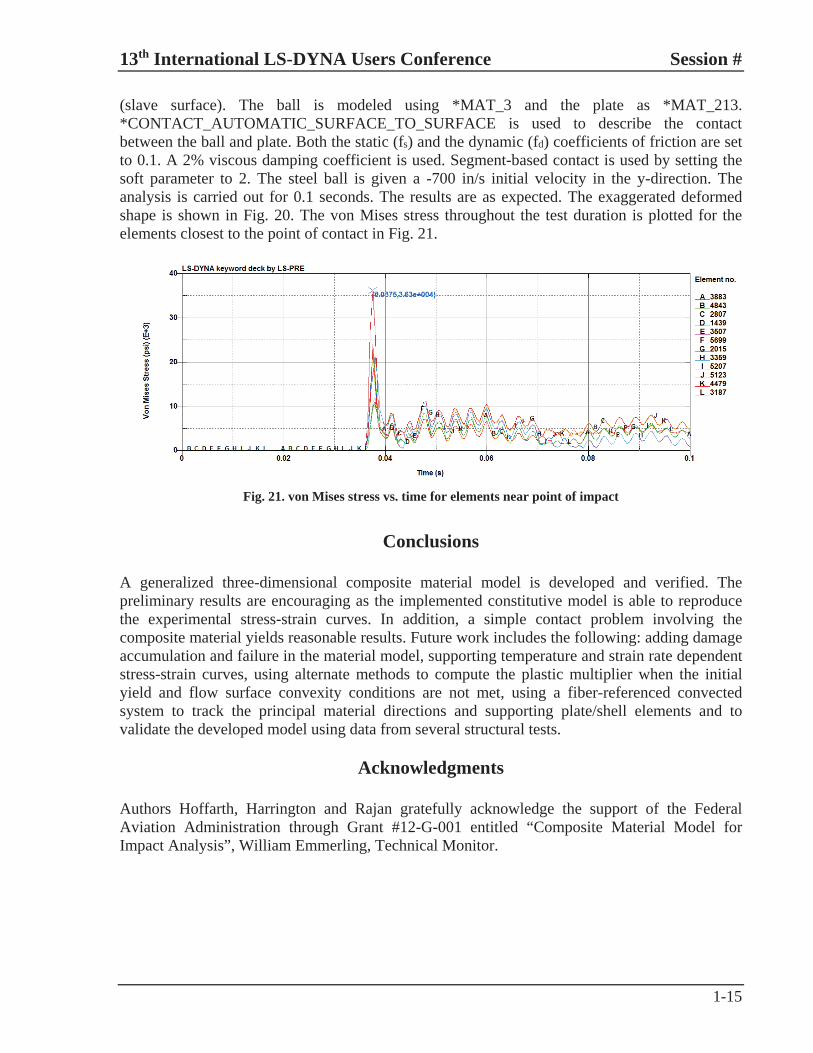
(slave surface). The ball is modeled using *MAT_3 and the plate as *MAT_213. *CONTACT_AUTOMATIC_SURFACE_TO_SURFACE is used to describe the contact between the ball and plate. Both the static (fs) and the dynamic (fd) coefficients of friction are set to 0.1. A 2% viscous damping coefficient is used. Segment-based contact is used by setting the soft parameter to 2. The steel ball is given a -700 in/s initial velocity in the y-direction. The analysis is carried out for 0.1 seconds. The results are as expected. The exaggerated deformed shape is shown in Fig. 20. The von Mises stress throughout the test duration is plotted for the elements closest to the point of contact in Fig. 21.

Fig. 21. von Mises stress vs. time for elements near point of impact

Conclusions A generalized three-dimensional composite material model is developed and verified. The preliminary results are encouraging as the implemented constitutive model is able to reproduce the experimental stress-strain curves. In addition, a simple contact problem involving the composite material yields reasonable results. Future work includes the following: adding damage accumulation and failure in the material model, supporting temperature and strain rate dependent stress-strain curves, using alternate methods to compute the plastic multiplier when the initial yield and flow surface convexity conditions are not met, using a fiber-referenced convected system to track the principal material directions and supporting plate/shell elements and to validate the developed model using data from several structural tests.

Acknowledgments Authors Hoffarth, Harrington and Rajan gratefully acknowledge the support of the Federal Aviation Administration through Grant #12-G-001 entitled “Composite Material Model for Impact Analysis”, William Emmerling, Technical Monitor.


1-16

References

[1] L. P. Moreira and G. Ferron, "Finite element implementation of an orthotropic plasticity model for sheet metal forming simulations," Latin American Journal of Solids and Structures, vol. 4, pp. 149-176, 2007. [2] M. Ganjiani, R. Naghdabadi and M. Asghari, "An elastoplastic damage-induced anisotropic constitutive model at finite strains," International Journal of Damage Mechanics, vol. 22, pp. 499-529, 2012. [3] J. S. Bergstrom, "Constitutive Modeling of Elastomers - Accuracy of Predictions and Numerical Efficiency," 2005. [Online]. Available: PolymerFEM.com. [4] A. Tabiei and J. Wu, "Three-dimensional nonlinear orthotropic finite element material model for wood," Composite Structures, vol. 50, pp. 143-149, 2000. [5] C. T. Sun and J. L. Chen, "A Simple Flow Rule for Characterizing Nonlinear Behavior of Fiber Composites," Journal of Composite Materials, 1989. [6] R. Vaziri, M. D. Olson and D. L. Anderson, "A Plasticity-Based Constitutive Model for Fibre-Reinforced Composite Laminates," Journal of Composite Materials, pp. 512-535, 1991. [7] G. A. Holzapfel and T. C. Gasser, "A viscoelastic model for fiber-reinforced composites at finite strains: Continuum basis, computational aspects and applications," Computer methods in applied mechanics and engineering, vol. 190, pp. 4379-4403, 2001. [8] P. B. Lourenco, R. D. Borst and J. G. Rots, "A Plane Stress Softnening Plasticity Model for Orthotropic Materials," International Journal for Numerical Methods in Engineering, pp. 4033-4057, 1997. [9] Y. D. Murray and L. E. Schwer, "Verification of a general-purpose laminated composite shell element implementation: Comparisons with analytical and experimental results," Finite Elements in Analysis and Design, vol. 13, no. 1, pp. 1-16, 1993. [10] G. C. Saha and A. L. Kalamkarov, "Micromechanical Thermoelastic Model for Sandwhich Composite Shells made of Generally Orthotropic Materials," Journal of Sandwich Structures and Materials, vol. 11, pp. 27-56, 2009. [11] J. D. Littell, W. K. Binienda, W. A. Arnold, G. D. Roberts and R. K. Goldberg, "Effect of Microscopic Damage Events on Static and Ballistic Impact Strength of Triaxial Braid Composites," NASA, Washington, 2010. [12] A. Matzenmiller, J. Lubliner and R. L. Taylor, "A constitutive model for anisotropic damage in fiber-composites," Mechanics of Materials, vol. 20, pp. 125-152, 1995. [13] X. Xiao, "Modeling Energy Absorbtion with a Damage Mechanics Based Composite Material Model," Journal of Composite Materials, vol. 43, pp. 427-444, 2009. [14] F. Wu and W. Yao, "A fatigue damage model of composite materials," International Journal of Fatigue, pp. 134-138, 2010. [15] H.-S. Chen and S.-F. Hwang, "A Fatigue Damage Model for Composite Materials," Polymer Composites, pp. 301-308, 2009. [16] B. A. Gama, J.-R. Xiao, M. J. Haque, C.-F. Yen and J. W. J. Gillespie, "Experimental and Numerical Investigations on Damage and Delamination in Thick Plain Weave S-2 Glass Composites Under Quasi-Static Punch Shear Loading," U.S. Army Research Laboratory, Aberdeen Proving Ground, 2004. [17] A. F. Johnson, A. K. Pickett and P. Rozycki, "Computational methods for predicting impact damage in composite structures," Composites Science and Technology, vol. 61, pp. 2183-2192, 2001. [18] J. Ozbolt, V. Lackovic and J. Krolo, "Modeling fracture of fiber reinforced polymer," International Journal of Fracture, vol. 170, pp. 13-26, 2011. [19] C.-F. Yen, "Ballistic Impact Modeling of Composite Materials," in 7th International LS-DYNA Users Conference, 2002. [20] R. Goldberg, K. Carney, P. DuBois, C. Hoffarth, J. Harrington, S. Rajan and G. Blankenhorn, "Theoretical Development of an Orthotropic Three-Dimensional Elasto-Plastic Generalized Composite Material Model," in 13th International LS-DYNA User's Conference, Detroit, MI, 2014. [21] K. S. Raju and J. F. Acosta, "Crashworthiness of Composite Fuselage Structures - Material Dynamic Properties, Phase I," U.S. Department of Transportation: Federal Aviation Administration, Washington, DC, 2010. [22] D. L. Smith and M. B. Dow, "Properties of Three Graphite/Toughened Resin Composites," NASA Technical Paper 3102, September 1991. [23] B.A. Bednarcyk and S.M. Arnold, “MAC/GMC 4.0 User’s Manual - Keywords Manual,” NASA/TM-2002-212077/VOL2, National Aeronautics and Space Administration, Washington, D.C., 2002. [24] J. Harrington and S.D. Rajan, Test Results from Virtual Testing Software System, Technical Report, School of Sustainable Engineering and the Built Environment, ASU, March 2014. [25] J. Hallquist, LS-DYNA Keyword User’s Manual, Version 970. Livermore Software Technology Corporation, Livermore, CA, 2013.

verification and validation of a three-dimensional

Documents