verification document for ultramarine...
TRANSCRIPT

Ultramarine, inc.
VERIFICATION DOCUMENT FOR
ULTRAMARINE OFFSHORE SOFTWARE
Phone (713) 975-8146 Fax (713) 975-8179
Copyright Ultramarine, Inc. November 1985 and June 29, 2009

Contents
I. INTRODUCTION . . . . . . . . . . . . . . . . . . . . . . . . . 1II. REGULARATORY APPROVAL . . . . . . . . . . . . . . . . 2III. PERIODIC MOTION . . . . . . . . . . . . . . . . . . . . . . . 3IV. PLATE DEFORMATION . . . . . . . . . . . . . . . . . . . . 7V. HOOP STRESS IN A CYLINDER . . . . . . . . . . . . . . . 9VI. STRESS CONCENTRATION OF A CIRCULAR HOLE . . . 12VII. GENERALIZED DEGREES OF FREEDOM . . . . . . . . . . 15VIII. BEAM RESIZING . . . . . . . . . . . . . . . . . . . . . . . . 21IX. SIMPLE HYDROSTATICS . . . . . . . . . . . . . . . . . . . 22X. STRIP THEORY HYDRODYNAMICS . . . . . . . . . . . . . 27XI. THREE DIMENSIONAL DIFFRACTION HYDRODYNAMICS 32XII. HORIZONTAL OSCILLATION OF A TANKER . . . . . . . . 38XIII. WIND AND CURRENT FORCE . . . . . . . . . . . . . . . . 41XIV. PIPELAYING . . . . . . . . . . . . . . . . . . . . . . . . . . . 50XV. QUALITY ASSURANCE PROCEDURES . . . . . . . . . . . 51REFERENCES . . . . . . . . . . . . . . . . . . . . . . . . . . . . . . . . 54
Page i

I. INTRODUCTION
The purpose of this document is to provide information on the applicability of theresults produced by Ultramarine’s software, MOSES, to “real world” problems. Webegin by considering some simple problems where exact solutions are available. Manyproblems of interest, however, are not amenable to such checks. For these cases, weturn to comparisons with model tests and/or other computed results.
Although not strictly applicable, it should be mentioned that MOSES has beenaround in some incarnation since the late 1970’s and it has been used on hundreds ofprojects. This is, perhaps, the best statment for the accuracy and reliability of theresults it produces.
Because of the range of problems our software can solve, it is impossible to compareeverything. What we have here are enough comparisons to establish that the “ba-sic ingredients” function properly. Thus, they give comfort that MOSES functionsproperly for a much wider class of problem than covered here.
The document finishes with a description of our Quality Assurance procedures. Inessence, these procedures are designed to minimize the chance of errors creeping intothe software during the maintenance process.
MOSES Verification Page 1

II. REGULARATORY APPROVAL
One of the questions we are continually asked about is whether or not MOSES isapproved by some regulatory bodies such as ABS or DNV. The answer to this isno, regulatory bodies, in general, approve result and designs, not software. SinceMOSES has been in constant use for decades, literally hundreds of results have beenapproved by various regulatory bodies. Never have we heard of a case where a designor analysis was rejected because of the software used.
One exception that we know of to the above rule is that the Norweign PetroleumDirectoriat did (or does) approve combinations of organizations and software to per-form mooring and stability calculations. There are several organizations - MOSEScombinations which have been aproved.
MOSES Verification Page 2

III. PERIODIC MOTION
In this section we investigate two cases of periodic motion which can be comparedwith exact solutions. A simple spring-mass system is considered first, and then welook at the large motion of a pendulum. The primary objective is to examine howwell time domain problems can be solved. In particular, is appreciable numericaldamping induced into the solution, and are the nonlinearities properly accountedfor. The two samples chosen also address the question of how well flexible and rigidconnections function in the time domain.
The first test consists of a spring, modeled by a vertical bar with a Young’s modulusof 10 kips/in2, length of 100 ft., and a constant circular cross section of 1 ft. diameter.The block has a weight of 1000 kips as is shown in Figure 1. To initiate the motion,the mass was displaced by 10 ft. in the positive z-direction and released.
Figure 1: Setup for Spring Vibration
For uniaxial deformation, the deflection of the bar under load P is
δ =PL
AE, (III.1)
and the spring constant is
k =P
δ=AE
L. (III.2)
MOSES Verification Page 3

The quantities verified are the natural frequency, the force needed to stretch thespring 10 ft., and the stretched length of the spring with a 1000 kip block. The forcerequired to change the length of the bar 10 ft. can be determined by solving (III.1)for P ,
P =δEA
L(III.3)
which for a δ = 10ft and the bar particulars given above results in P = 113.09 Kips.The natural frequency and period of the system are given by
ωn =
√k
m, and (III.4)
T =2π
ωn
. (III.5)
Using these equations with the spring constant of 11.3 kips/ft given by (III.2) yieldsa natural period of 10.37 sec. The stretched length of the spring corresponds tothe average length of the spring during oscillation. In Figure 2 we show the meanoscillation being about z=-89 ft. Recalling that the spring is 100 ft. long at z=0 ft.will conclude that the springs stretched length is 189 ft. Again using (III.1) withthe weight of the block gives the stretched length of the bar to be 88.5 ft. from itsz=0 ft. position.
Below we present the comparison of hand calculated values to those from MOSES.As can be seen there is a good comparison between the force needed to move theblock to z=10 ft., the natural period, and the stretched length. The force to movethe block to z=10 ft. was taken from the MOSES status report, the mean z-locationwas taken from the statistics of the block motion, and the natural period was takenfrom the plot of oscillatory motion for 100 sec. Finally, notice that the numericalintegration did not induce any perceptible error.
Comparison of Exact Solution and MOSES for Spring-Mass System
Quantity units Hand MOSES
Force to move to z=10 ft. kips 113.00 113.00Natural period sec. 10.41 10.40Z-Mean ft. 88.50 88.42
Next we consider the large angular motion of a pendulum. This is by far the moreinteresting of the two tests, since the governing equation is nonlinear. The systemconsists of a 100 ft. bar of constant section, hinged at one end. The bar is initiallyrotated 90 degrees and released.
MOSES Verification Page 4

CGMean
Verification of Natural Frequency
0 10 20 30 40 50 60 70 80 90 100
Time (Seconds)
-190
-170
-150
-130
-110
-90
-70
-50
-30
-10
10Z
Loc
atio
n (f
t)
Figure 2: Vibration of Spring-Mass System
The equation of motion for the pendulum in terms of the angle, θ, mass, m, lengthof bar, l, and moment of inertia, Io is
θ + ω2 sin θ = 0 , (III.6)
where
ω2 =3g
2l, (III.7)
and g is the acceleration of gravity. The period for motion satisfying this equation isan elliptic integral and can be represented as
T =2
πK(2πω) (III.8)
where K is dependent on the initial amplitude. For 90 degrees K = 1.854 whichyields a period of T = 10.66 sec. As can be seen from Figure 3 the computed resultshave a period which is the same as the predicted value. It is also worth noting theplateaus in the acceleration vs. time plot shown in Figure 4. The motion here iscertainly not described by a cosine.
MOSES Verification Page 5

Sample Of a Simple Pendulum
0 2.1 4.2 6.3 8.4 10.5 12.6 14.7 16.8 18.9 21
Time (Seconds)
-90
-72
-54
-36
-18
018
3654
7290
Rol
l Ang
le (
Deg
)
Figure 3: Oscillation of Pendulum Motion
Sample Of a Simple Pendulum
0 2.1 4.2 6.3 8.4 10.5 12.6 14.7 16.8 18.9 21
Time (Seconds)
-28
-22.
4-1
6.8
-11.
2-5
.60
5.6
11.2
16.8
22.4
28R
oll A
ngul
ar A
ccel
erat
ion
(Deg
/Sec
^2)
Figure 4: Acceleration of Pendulum Motion
MOSES Verification Page 6

IV. PLATE DEFORMATION
In this section we consider the deformation of a cantelever plate due to uniaxialloading and pure bending. The deformation of the cantelever is simple enough so thatMOSES results can be easily compared. We considered three plate models. In allthree models the main dimensions of the cantelever remained the same, however therefinement of the sections considered was changed. This example not only illustrateshow the plate element is used, but demonstrates how accuracy is increased withdetail.
There were three models considered: a single plate, a plate refined along the y-axis,and a plate refined along both the y-axis and the x-axis. For all three cases therewas an axial force in the negative x-direction, a shear load in the negative z-directionand a shear load in the negative y-direction. These three cases are shown in Figure5. The dimensions of the plate are length of 10 ft., width of 4 ft., and thickness of 1in.
The equations that govern the deformation of the plate are:
δx =f`
EA,
δy =P`3
3EIyy
,
δz =P`3
3EIzz
, (IV.1)
where
A = wt ,
Iyy =tw3
12, and
Izz =wt3
12. (IV.2)
The comparison of MOSES values to hand calculated values is shown in below. Animportant thing to notice about these results is the dramatic improvement of δy withrefinement. A single plate element is simply incapable of representing global bendingdue to membrane stresses.
MOSES Verification Page 7

Plate Deformation with Different Models
Hand MOSES MOSES MOSESCalculations Uniform Sliced Diced
δx (in.) 0.086 0.086 0.086 0.087δy (in.) 0.215 0.058 0.162 0.235δz (in.) 4.966 4.646 4.928 4.768
Figure 5: Plate refinement models
MOSES Verification Page 8

V. HOOP STRESS IN A CYLINDER
In this section, we will investigate how well MOSES computes the hoop stresses ina thin-walled cylindrical shell due to external pressure. Here, we consider a cylinderwith the radius r=31.5 ft., thickness t=1 in., and total length `= 300 ft. The cylinderwas submerged 295 ft. with no trim or heel.
Since MOSES employs a finite element method, the answer will depend on howaccurately we model the cylinder. Thus, results for four models were obtained: twomodels with the nodes on the perimeter of the cylinder and two with a distance fromthe center that preserves the area. For each scheme of placing the nodes, modelsof 8 and 16 plates around the circumference were created. Plots of the modes areshown below. Notice that to preserve the area, a different distance is needed for eachnumber of plates:
d =
√√√√ 2πr2
n sin(2πn
)
For the r we have, this corresponds to d=33.2 ft. for 8 plates and d=31.91 ft. for 16plates. Figures 6 through 8 show the geometric difference in detail.
Figure 6: Top View of Simple Models
The ”standard results” are given by:
σr = 0 ,
MOSES Verification Page 9

Figure 7: Top View of Detail Models
Figure 8: Side View of Detail Models
MOSES Verification Page 10

σθ =Pr
t,
σz =Pr
2t,
P = −ρgh . (V.1)
Here, σr is the radial stress, σθ is the tangential stress, σz is the longitudinal stress,r is the inner radius, t is the shell thickness, P is the pressure, ρ is the density ofwater, g is the gravitational constant, and h is the water depth of the point beingmeasured.
Membrane Stess of a Thin Walled Cylindrical Shell
σθ σz
Standard Formulae -49.35 -24.688 Plates on Perimeter -43.93 -21.378 Plates Preserve Area -46.28 -22.5216 Plates on Perimeter -47.65 -23.4916 Plates Preserve Area -48.26 -23.80
It is interesting that the results for the equivalent area models are substantially betterthan the ones from the perimeter models. Also, the results are surprisingly close forsuch crude models.
MOSES Verification Page 11

VI. STRESS CONCENTRATION OF A CIRCULAR HOLE
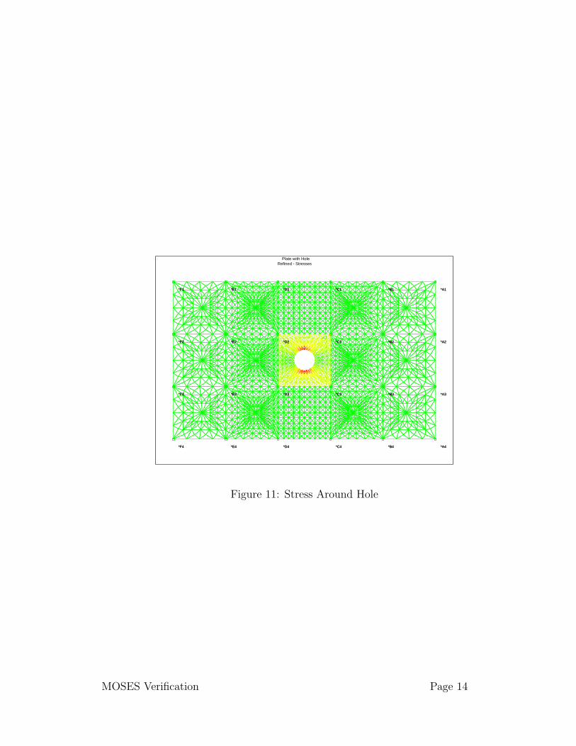
In this section we consider the stress concentration factor for a circular hole in a platesubjected to ”uniform” tension. Figure 9 shows the plates as defined and Figure 10shows the refined mesh of 2732 nodes which is actually used to solve for the stressesaround the hole.
*A1
*A2
*A3
*A4
*B1
*B2
*B3
*B4
*C1
*C2
*C3
*C4
*D1
*D2
*D3
*D4
*E1
*E2
*E3
*E4
*F1
*F2
*F3
*F4
*A1
*A2
*A3
*A4
*B1
*B2
*B3
*B4
*C1
*C2
*C3
*C4
*D1
*D2
*D3
*D4
*E1
*E2
*E3
*E4
*F1
*F2
*F3
*F4
Plate with HoleOriginal Mesh
Figure 9: Original Model
Loads are applied to the left edge of the model and the right edge of the model isrestrained. The total load applied is 1200 kips and this yields a nominal stress of 3.33ksi. Figure 11 shows the stress distribution around the hole. The maximim stresshere is 10.08 giving a stress concentration factor of 3.02 which compares quite nicelywith the correct value of 3.
MOSES Verification Page 12

*A1
*A2
*A3
*A4
*B1
*B2
*B3
*B4
*C1
*C2
*C3
*C4
*D1
*D2
*D3
*D4
*E1
*E2
*E3
*E4
*F1
*F2
*F3
*F4
*A1
*A2
*A3
*A4
*B1
*B2
*B3
*B4
*C1
*C2
*C3
*C4
*D1
*D2
*D3
*D4
*E1
*E2
*E3
*E4
*F1
*F2
*F3
*F4
Plate with HoleHole Refined
Figure 10: Refined Model
MOSES Verification Page 13
*A1
*A2
*A3
*A4
*B1
*B2
*B3
*B4
*C1
*C2
*C3
*C4
*D1
*D2
*D3
*D4
*E1
*E2
*E3
*E4
*F1
*F2
*F3
*F4
*A1
*A2
*A3
*A4
*B1
*B2
*B3
*B4
*C1
*C2
*C3
*C4
*D1
*D2
*D3
*D4
*E1
*E2
*E3
*E4
*F1
*F2
*F3
*F4
Plate with HoleRefined - Stresses
Figure 11: Stress Around Hole
MOSES Verification Page 14

VII. GENERALIZED DEGREES OF FREEDOM
MOSES’s generalized degrees of freedom was designed to solve problems that reallyare not solvable by any other means, and as a result, this capability is not easy tocheck. Our approach here is to construct an estimate of the solution to a problem,check the estimate where it can be checked, and then compare it with MOSES. Inparticular, we want to solve a ”flag pole”, a vertical beam with a weight on top,and we will compare the MOSES results to this problem with a standard energyapproximation; i.e. we will look at energy in the beam system:
K =ρ
2
∫ `1+`2
0x2 dz +
1
2
W
gx(`1 + `2)
2 ,
V1 =1
2EI
∫ `1+`2
0(x′′)2 dz ,
V2 ≈ −W2
∫ `1+`2
0(x′)2 dz and
W =∫ `1+`2
0F (z)x dz . (VII.1)
Here, the first term of K is the kinetic energy of the beam itself, the second is thekinetic energy of the weight on the top, V1 is the strain energy due to bending thebeam, V2 is the potential energy due to the weight at the top, and W is the workdone by forces acting along the beam. We will consider the beam to be ”pinned” atz = 0 and z = `1, so we really have a two span beam which approximates a cantileverwhen `1 is small in comparison to `1 + `2.
Now, assume x(z) is a function with continuous derivatives, satisfies the boundaryconditions, and depends on a single parameter δ, the value at z= `1 + `2. Then
K = −1
2(δ)2
(ρ∫ `1+`2
0x2 dz +
W
g
)≡ 1
2(δ)2M ,
V1 =1
2(δ)2EI
∫ `1+`2
0(x′′)2 dz ≡ 1
2(δ)2K1 ,
V2 =1
2− (δ)2(W
∫ `1+`2
0(x′)2 dz ≡ −1
2(δ)2 1
2K2 and
W = δ
(Fo +
∫ `1+`2
0fx2 dz
)≡ δ(Fo + C) . (VII.2)
Here, Fo is a force applied at the top of the beam and C is a contribution due to aforce, f , acting along the beam.
If we now look at conservation of energy, we get an equation
K + V1 + V2 =W (VII.3)
MOSES Verification Page 15

which, if we use (VII.3) and differentiate with respect to time, yields
Mδ + (K1 −K2)δ=Fo + C .
Now, let us assume that δ, Fo, and C are harmonic in time with frequency ω, whichwill reduce the above equation to an algebraic one:
−ω2δM + (K1 −K2)δ=Fo + C
or
δ=Fo + C
[−ω2M + (K1 −K2)]. (VII.4)
If we have computed the integrals K1, K2, C, and M then (VII.4) provides anestimate of the deflection at the top of our beam.
Before attaching the integrals, let us first look at some special cases of verify:1. First,notice that it does not have a solution when
ω2 =K1 −K2
M
which gives us an estimate of the natural frequency of the beam. Also, notice thatwhen C = 0 and ω = 0, it yields
δ=Fo
(K1 −K2)
which is the static deflection due to a load applied at the top. These two results willbe used to check the accuracy of this approximation. Since (VII.4) has a singularityat the natural period, we will alter it slightly with a bit of damping
δ=Fo + C√
[−ω2M + (K1 −K2)]2 + 4η2(K1 −K2)M
. (VII.5)
We are still free to chose any x which satisfies the boundary conditions:
x(`1) = 0lim
z→`+1
x′(z) = limz→`−1
x′(z)
x′′(`1) = 0x(`1 + `2) = 1x′′(`1 + `2) = 0 . (VII.6)
Our choice is the static deflection under a top load:
x=
{αz + βz3, z ≤ `1;γ(z − `1) + ψ(z − `1)
2 + ζ(z − `1)3, z > `1
(VII.7)
MOSES Verification Page 16

where the parameters α, β, γ, ψ,and ζ can be determined from the above boundaryconditions.
The particular problem we consider is a tube with:
`1 = 10 meters,`2 = 90 meters,W = 100 kilo-newtons,Fo = 10 kilo-newtons, (VII.8)
and which has a diameter of 1 meter and a thickness of 25 millimeters. The buoyancyof the tube was chosen to be equal the weight so that we did not have to include thepotential energy of either the weight or the buoyancy of the tube in our equation.When the tube is in the water, the density used above includes both the densityof the steel in the tube and the added mass. Also, the integral C is the Morison’sequation inertia force due to wave particle acceleration.
Comparing the results of our approximation with the results from a stress analysiswe find
Comparison of Energy Approximation with Structural Analysis
Quantity units W Structural Energy App.
Deflection due to Fo Meters 0. 1.484 1.484Deflection due to Fo Meters 10. 1.484 1.836Natural period in Air sec. 0. .476 .468Natural period in Water sec. 0. 12.785 12.920Natural period in Water sec. 10. 12.785 14.220
These comparisons are interesting. First, the comparisons with W = 0 are excellent,but those for a nonzero weight are not so good. This is due to the fact that thestructural analysis we are comparing with is linear; i.e. the effect of the weight onthe stiffness is not accounted for. Thus, for these cases the estimate is itmore correctthan the stress analysis.
Since the estimate is reasonably reliable, we can turn to a comparison of the resultsfrom MOSES generalized coordinates and the estimate. We first computed threemodes of the beam in water using the pin connections and then used these as gen-eralized coordinates. The following two figures show a comparison of the resultsboth with a weight and without. As you can see, MOSES does quite a nice job ofpredicting the response including the nonlinearities.
One must be a bit careful using generalized coordinates. Above, we had a set ofmodes which exactly satisfied the boundary conditions. To show what can happen
MOSES Verification Page 17

if you do not have a ”good set” of modes, we also solved the same problem with a”bad” set of modes. These ”bad” modes are backward; i.e. they correspond to abeam fixed at the top! The second set of figures show the results using two of thesemodes and twenty of them. As you can see, with two modes, you have a really badestimate of the deformation, while with twenty it is not so bad.
Figure 12: Frequency Response with No Weight
MOSES Verification Page 18

Figure 13: Frequency Response with Weight
Figure 14: Two ”Bad” Modes
MOSES Verification Page 19

Figure 15: 20 ”Bad Modes
MOSES Verification Page 20

VIII. BEAM RESIZING
In this section we present the beam resizing option. Several examples illustratinghow the algorithm works are included as samples of MOSES to show the procedureused for resizing. All resizing samples are taken from classic textbook examples. Abrief explanation of each sample follows.
Gaylord and Gaylord, Design of Steel Structures, Example 5-12, DP5-2: Crane forshop building. Given the length and the load of the bridge and the girder, determinethe size of the beams needed.Root filename: resiz1
Salmon and Johnson, Steel Structures Design and Behavior, Example 15.4.1. Designa rectangular frame of 75-ft. span and 25-ft. height to carry a gravity uniform loadof 1.0 kip/ft. when no lateral load is acting.Root filename: resiz2
AISC Manual of Steel Construction beam Examples 1-3, p. 2-5 through 2-6. Design abeam subjected to a given bending moment and a specific compressions flange braceintervals.Root filename: resiz3
AISC Manual of Steel Construction beam Example 1, p. 3-4. Given a concentricload and the effective length with respect to the minor axis, determine the size of thebeam needed.Root filename: resiz4
AISC Manual of Steel Construction beam Example 10, p. 2-147. Given the load ona girder, the distance from the ends reaction points, and the moment at the center,determine the girder size.Root filename: resiz5
The user is asked to use the samples provided and the references to supplement thissection of the verification manual.
MOSES Verification Page 21

IX. SIMPLE HYDROSTATICS
In this section, we consider the hydrostatic properties of two simple bodies, a cubeand a tube. These bodies are simple enough so that exact calculations can be made,and MOSES uses two different algorithms for the two cases. Thus, they provide anexcellent check of the hydrostatics for any body.
The cube was considered in three positions: trimmed, heeled, and both trimmed andheeled. The side of the cube has length of ` = 50ft., and a draft T which is measuredperpendicular to the waterplane from the deepest submerged point of the body. Theequations for the center of buoyancy for the trimmed position and for the heeledposition were derived from the center of mass equations of a wedge.
The equations for the center of buoyancy and displacement in a trimmed position areas follows:
Xcb =2T
3 sinφ,
Ycb =1
2l ,
Zcb =T
3 cosφ, and
∆ = ρlT 2
sin 2φ. (IX.1)
For a heeled position, the equations become:
Xcb =1
2l ,
Ycb =2T
3 sin θ,
Zcb =T
3 cos θ, and
∆ = ρlT 2
sin 2θ. (IX.2)
The equations for the center of buoyancy of a trimmed and heeled box are morecomplicated since two rotations are taking place. It is simple to see that the volumeof a cube for a draft, T ≤ l sin θ cosφ which has been rotated about the y-axis by anangle θ then rotated about the x-axis an angle φ will resemble a tetrahedron. Thefollowing equations determine the center of buoyancy and the
Xcb = l− T
4 sinφ,
MOSES Verification Page 22

Ycb =T
4 cosφ cos θ,
Zcb = l− T
4 cosφ sin θ, and
∆ =ρT 3
(1000)(6) sinφ cos2 φ sin θ cos θ. (IX.3)
The coordinate systems are shown in Figures 16, 17 and 18. The global coordinatesystem with its x-y plane on the waterplane is shown as the coordinate system with-out primes, and the body coordinate system belonging to the cube is shown as thecoordinate system with primes.
Figure 16: Side View of Cube Position 1
These equations were used to compute the center of buoyancy and the displacementof the cube for the three positions.
MOSES Verification Page 23

Figure 17: Front View of Cube Position 2
Figure 18: Isometric View of Cube Position 3
MOSES Verification Page 24

Comparison of Hydrostatics of a Cube
Position Draft Trim Roll Method ∆ Xcb Ycb Zcb
ft. Deg Deg Kips ft. ft. ft.
1 25.00 30 00 Hand 2309.40 33.33 25.00 9.63MOSES 2309.40 33.33 25.00 9.62
2 35.35 00 45 Hand 4000.00 25.00 33.33 16.67MOSES 4000.00 25.00 33.33 16.67
3 30.61 30 45 Hand 889.12 37.50 39.79 10.21MOSES 889.80 37.50 39.79 10.21
Next, we consider the hydrostatics of a tube in three conditions. The tube is 50 ft.long with a radius of 5 ft. Here θ is a pitch angle measured from the global z-axisto the body z’-axis. For these tests, draft is defined as the vertical distance from thebody coordinate system to the mean water level. The geometry is shown in Figure19, and body coordinate system is denoted as the x’-z’ axis.
Figure 19: Coordinate System for Buoyancy of a Tube
The buoyancy and its center are determined by integration of the following equations:
v =∫
Sdv
MOSES Verification Page 25

∆ = ρgv
Xcb =1
v
∫Sx dv
Ycb =1
v
∫Sy dv
Zcb =1
v
∫Sz dv (IX.4)
Here, S is the submerged portion of the tube. The comparison for three cases is:
Comparison of Hydrostatics of a Tube
Position Draft Trim Roll Method ∆ Xcb Ycb Zcb
ft. Deg Deg Kips ft. ft. ft.
1 34.64 00 30 Hand 201.09 0.18 0.00 20.09MOSES 201.06 0.09 0.00 20.03
2 0.00 60 00 Hand 9.24 2.55 0.00 2.98MOSES 9.24 2.50 0.00 2.95
3 0.00 80 00 Hand 30.25 2.92 0.00 8.40MOSES 30.25 2.95 0.00 8.35
MOSES Verification Page 26

X. STRIP THEORY HYDRODYNAMICS
In this section, we compare the RAOs of a barge from a study conducted by NobleDenton and Associates Ltd. [1] and those computed by MOSES using strip theory.The model studied is a deck barge of dimensions depicted in Figure 20, with a KGof 32 ft.
Comparison of MOSES Strip Theory w/Model TestsEvent 1.0
Figure 20: Barge Particulars
The comparisons are shown in Figures 21 to 26. The Noble Denton report consistedof RAO curves with an average of 5 data points per degree of freedom. The datapoints were from measurements of a 1:30 ratio model in regular waves for head andbeam seas. Surge and heave motions were recorded for head seas and sway, heave,and roll motions were recorded for beam seas. The points recorded by Noble Dentonare indicated in each curve by circles. Points with a “W” indicate that for this test,the deck of the barge was awash.
The MOSES curves were calculated with a wave steepness of 1/20. As seen fromthese figures, most of the computed RAOs compare quite well with those from themodel test. The only exception is the roll RAOs, in which case the computed resultsdeviate from the test results near resonance. This is due to nonlinear roll dampingwhich causes the response near resonance to be greatly affected by the wave steepness.To address this nonlinearity, roll response curves were calculated for a range of wavesteepnesses. These results are shown in Figure 26. In this figure, the MOSES results
MOSES Verification Page 27

are shown with wave steepness decreasing from 1/133 to 1/33. These wave steepnesseswere chosen in order to correspond with those steepnesses tested by Noble Denton.The graph shows an agreement between test measurements and MOSES results.
MosesModel Test
Comparison of MOSES Strip Theory w/Model Tests405x90x20 ft Barge, 9.0ft draft, Head Seas
4 5.6 7.2 8.8 10.4 12 13.6 15.2 16.8 18.4 20
Period, Sec
00.
10.
20.
30.
40.
50.
60.
70.
80.
91
Sur
ge, f
t/ft
Figure 21: Comparison of Surge RAO in Head Seas
MOSES Verification Page 28

MosesModel Test
Comparison of MOSES Strip Theory w/Model Tests405x90x20 ft Barge, 9.0ft draft, Head Seas
4 5.6 7.2 8.8 10.4 12 13.6 15.2 16.8 18.4 20
Period, Sec
00.
10.
20.
30.
40.
50.
60.
70.
80.
91
Hea
ve, f
t/ft
Figure 22: Comparison of Heave RAO in Head Seas
MosesModel Test
Comparison of MOSES Strip Theory w/Model Tests405x90x20 ft Barge, 9.0ft draft, Head Seas
4 5.6 7.2 8.8 10.4 12 13.6 15.2 16.8 18.4 20
Period, Sec
00.
040.
080.
120.
160.
20.
240.
280.
320.
360.
4P
itch
deg/
ft
Figure 23: Comparison of Pitch RAO in Head Seas
MOSES Verification Page 29

MosesModel Test
Comparison of MOSES Strip Theory w/Model Tests405x90x20 ft Barge, 9.0ft draft, Beam Seas
5 6.5 8 9.5 11 12.5 14 15.5 17 18.5 20
Period, Sec
00.
150.
30.
450.
60.
750.
91.
051.
21.
351.
5S
way
, ft/f
t
Figure 24: Comparison of Sway RAO in Beam Seas
MosesModel Test
Comparison of MOSES Strip Theory w/Model Tests405x90x20 ft Barge, 9.0ft draft, Beam Seas
5 6.5 8 9.5 11 12.5 14 15.5 17 18.5 20
Period, Sec
00.
150.
30.
450.
60.
750.
91.
051.
21.
351.
5H
eave
, ft/f
t
Figure 25: Comparison of Heave RAO in Beam Seas
MOSES Verification Page 30

Moses Roll S33Moses Roll S52Moses Roll S75Moses Roll S133Model Test
Comparison of MOSES Strip Theory w/Model Tests405x90x20 ft Barge, 9.0ft draft, Beam Seas
5 6.5 8 9.5 11 12.5 14 15.5 17 18.5 20
Period, Sec
00.
81.
62.
43.
24
4.8
5.6
6.4
7.2
8R
oll d
eg/ft
Figure 26: Comparison of Roll RAO in Beam Seas
MOSES Verification Page 31

XI. THREE DIMENSIONAL DIFFRACTION HYDRODY-NAMICS
In this section, we will examine three dimensional diffraction results for semisub-mersible vessel motions, comparing MOSES to the NSMB motions programs andto the model test results taken at NSMB [3]. It should be noted that NSMB, anacronym for Netherlands Ship Model Basin, is the former name for MARIN, Mar-itime Research Institute Netherlands.
The vessel used was the semisubmersible crane vessel Balder, with length, breadthand depth dimensions of 118 x 86 x 42 meters, respectively, at a 22.5 meter draft.Before comparison, the differences in the mathematical and test basin models shouldbe noted. The displacement computed by MOSES was 3.3 percent greater thaneither NSMB model, and the MOSES KG was 1.87 meters lower than NSMB’s. TheKG shift was necessary in order to achieve equivalent transverse GM values. Theseindicate different values of waterplane inertia, which cannot be compared since theywere not published in the NSMB report. Figures 27 illustrates the hydrostatic modelused by MOSES.
Figure 27: Isometric view of mesh model
This mesh was automatically refined by the program to generate a detailed mesh forhydrodynamics, as seen in Figure 28 Imposing a constraint that the maximum panelside be less than four meters resulted in a diffraction mesh of 1130 panels. For the
MOSES Verification Page 32

MOSES analysis, viscous damping was introduced by Morison tubular elements whichattract only drag forces. Diameters for these tubulars were chosen to approximatethe cross section of the pontoons and columns.
Comparison of MOSES Diffraction w/ Model TestsSemisubmersible Balder, 22.5M Draft
Event 1.0
Figure 28: Isometric view of detailed mesh model
The response operators for head, quartering, and beam seas are shown in Figures 29through 36 for periods up to 18 second. The legend in these figures label results fromMOSES (MO), NSMB diffraction program (Nd) and NSMB model tests (Nt). Thelabels X, Y, Z, RX, RY refer to surge, sway, heave, roll and pitch, respectively, whilethe values of 180, 135 and 90 refer to head seas, quartering seas and beam seas. Theagreement here is excellent.
MOSES Verification Page 33

MOSES RESULTSNSMB DIFFRACTIONNSMB TESTS
Comparison of MOSES Diffraction w/ Model TestsSemisubmersible Balder, 22.5M Draft, Head Seas
6 7.2 8.4 9.6 10.8 12 13.2 14.4 15.6 16.8 18
Period
00.
090.
180.
270.
360.
450.
540.
630.
720.
810.
9S
urge
RA
O (
M/M
)
Figure 29: Surge comparison in head seas
MOSES RESULTSNSMB DIFFRACTIONNSMB TESTS
Comparison of MOSES Diffraction w/ Model TestsSemisubmersible Balder, 22.5M Draft, Head Seas
6 7.2 8.4 9.6 10.8 12 13.2 14.4 15.6 16.8 18
Period
-0.1
-0.0
10.
080.
170.
260.
350.
440.
530.
620.
710.
8"H
eave
RA
O (
M/M
)’
Figure 30: Heave comparison in head seas
MOSES Verification Page 34

MOSES RESULTSNSMB DIFFRACTIONNSMB TESTS
Comparison of MOSES Diffraction w/ Model TestsSemisubmersible Balder, 22.5M Draft, Head Seas
6 7.2 8.4 9.6 10.8 12 13.2 14.4 15.6 16.8 18
Period
-0.1
-0.0
20.
060.
140.
220.
30.
380.
460.
540.
620.
7"P
itch
RA
O (
Deg
/M)’
Figure 31: Pitch comparison in head seas
MOSES RESULTSNSMB DIFFRACTIONNSMB TESTS
Comparison of MOSES Diffraction w/ Model TestsSemisubmersible Balder, 22.5M Draft, Quartering Seas
6 7.2 8.4 9.6 10.8 12 13.2 14.4 15.6 16.8 18
Period
-0.1
-0.0
20.
060.
140.
220.
30.
380.
460.
540.
620.
7"R
oll R
AO
(D
eg/M
)’
Figure 32: Roll comparison in quartering seas
MOSES Verification Page 35

MOSES RESULTSNSMB DIFFRACTIONNSMB TESTS
Comparison of MOSES Diffraction w/ Model TestsSemisubmersible Balder, 22.5M Draft, Quartering Seas
6 7.2 8.4 9.6 10.8 12 13.2 14.4 15.6 16.8 18
Period
-0.1
-0.0
30.
040.
110.
180.
250.
320.
390.
460.
530.
6"P
itch
RA
O (
Deg
/M)’
Figure 33: Pitch comparison in quartering seas
MOSES RESULTSNSMB DIFFRACTIONNSMB TESTS
Comparison of MOSES Diffraction w/ Model TestsSemisubmersible Balder, 22.5M Draft, Beam Seas
6 7.2 8.4 9.6 10.8 12 13.2 14.4 15.6 16.8 18
Period
00.
090.
180.
270.
360.
450.
540.
630.
720.
810.
9"S
way
RA
O (
M/M
)’
Figure 34: Sway comparison in beam seas
MOSES Verification Page 36

MOSES RESULTSNSMB DIFFRACTIONNSMB TESTS
Comparison of MOSES Diffraction w/ Model TestsSemisubmersible Balder, 22.5M Draft, Beam Seas
6 7.2 8.4 9.6 10.8 12 13.2 14.4 15.6 16.8 18
Period
00.
090.
180.
270.
360.
450.
540.
630.
720.
810.
9"H
eave
RA
O (
M/M
)’
Figure 35: Heave comparison in beam seas
MOSES RESULTSNSMB DIFFRACTIONNSMB TESTS
Comparison of MOSES Diffraction w/ Model TestsSemisubmersible Balder, 22.5M Draft, Beam Seas
6 7.2 8.4 9.6 10.8 12 13.2 14.4 15.6 16.8 18
Period
-0.1
-0.0
10.
080.
170.
260.
350.
440.
530.
620.
710.
8"R
oll R
AO
(D
eg/M
)’
Figure 36: Roll comparison in beam seas
MOSES Verification Page 37

XII. HORIZONTAL OSCILLATION OF A TANKER
In this section, we compare MOSES predictions for the motions of a tanker on asingle point mooring with those of Wichers [4]. The system consists of a ballasted200 Kdwt tanker with a 90 m hawser connecting it to the single point. The SPMsystem is exposed to 60 knot head winds and a 1.03 m/sec. head current. Thecoordinate system used is shown in Figure 37. The global coordinate system is fixedto earth, and head seas are defined as the environment in the positive x-direction.Also shown in Figure 37 is the top view of the panel model used for the 200 Kdwttanker.
Figure 37: Coordinate system
The MOSES simulation consisted of 1700 sec. at 2 sec. intervals. Figures 38 and 39show the x and y motions vs. time for: the model tests, the simulation conductedby Dr. Wichers, and the MOSES simulation. These results are quite interesting inthat we have an unsteady motion of the system in an environment which is constant.In other words, what we see here is the result of an instability. In view of this, thecloseness of the three results is quite remarkable. Wichers used experimental resultsto obtain coefficients in his simulation. For the MOSES simulation, the wind andcurrent forces were computed using the #tanker load group and nothing else wasdone.
Perhaps of even greater interest here is the variation of the tanker yaw angle with
MOSES Verification Page 38

Figure 38: Comparison of x motions
Figure 39: Comparison of y motions
MOSES Verification Page 39

time. This is shown in Figure 40.
Figure 40: Yaw motion for Single point mooring
MOSES Verification Page 40

XIII. WIND AND CURRENT FORCE
In this section, we consider the ways in which MOSEScomputes wind and currentforces. In essence, there are five ways: Morrison’s Equation for a tube (#TUBE),Morrison’s Equation for a plate (#PLATE), using the panels of a ”Piece” (closedsurface producing buoyancy and hydrodynamics), #TABLE, and #TANKER. Themathematics of computing the force for the first three load attractors is the same forwind and for current and for each of the elements. The only difference is in how the”drag coefficient” vector is defined. In what follows we will use a vector c which, ingeneral, can be defined as:
c = (Cx, Cy, Cz) (XIII.1)
For both plates and tubes, all values are the same and are specified with a MOSES&PARAMTER setting. For tubes, the coefficients for wind forces are specified with-WCSTUBE and for water forces with a Reynolds’ number dependent table specifiedwith -DRGTUB. For plates, it is specified with -DRGPLA for both wind and water.For panels, these are defined with the options -CS WIND and -CS CURR on eitherthe PGEN or PIECE command.
The force on each panel is computed as
f = sq(e·r)e (XIII.2)
Where f is the force vector, e is a unit vector, r is the relative velocity vector , ands and q are multipliers. Here s is given by
s= .5ρA ‖ r ‖ (XIII.3)
where ρ is the density of of the fluid, A is an area, and the last term is the relativespeed. The multiplier q is given by
q=∑
i
[c(i)n(i)r(i)] (XIII.4)
where n is the normal to the area and c(i) are the components of the c vector.
The meaning of A and e depend on the current setting of a MOSES parameterspecified with -AF ENVIRONMENT. If you use YES then
e = r/ ‖ r ‖A = a(n·r)/ ‖ r ‖ (XIII.5)
where a is the area of the panel or diameter times the length of a tube. If NO wasused, then
e = n
MOSES Verification Page 41

A = a (XIII.6)
his means the in the first case the force will be in the direction of the relative velocitywhile in the second it is normal to the area.
To see how the forces on panels works, we looked at the forces on the three shapesshown in Figure 41.
Comparison of Wind/Current ForceBodies Used
Event 1.0
Figure 41: Definitions of Shapes
Figures 42 - 44 show the surge, sway, current force and the magnitude of the force(‖ f ‖) on each of the shapes. Here, the force is computed using the MOSES Method,-AF ENVIRONMENT NO.
The thing to notice here is that the force depends on the shape; i.e. by integratingthe force over the the body you get a dependence of the force on the shape of thepiece. For head and beam currents, one gets a force of π/4 times that of the square.Thus if you want half that of a square you need to specify .5/.785 for the for Cx andCy.
One should notice that the directional behavior for the wind is identical to the currentso only one of them is presented here. Now, notice that the magnitude of the forceon both the tube and the square are independent of angle. This is a direct result ofthe fact that the x and y projected areas are the same and the force computation
MOSES Verification Page 42

RoundSquareWedge
Computed via MOSES MethodX Component of Current Force
0 18 36 54 72 90 108 126 144 162 180
Heading (Deg)
-130
-104
-78
-52
-26
026
5278
104
130
For
ce (
kips
)
Figure 42: Current Surge Force
RoundSquareWedge
Computed via MOSES MethodY Component of Current Force
0 18 36 54 72 90 108 126 144 162 180
Heading (Deg)
-130
-116
-102
-88
-74
-60
-46
-32
-18
-410
For
ce (
kips
)
Figure 43: Current Sway Force
MOSES Verification Page 43

RoundSquareWedge
Computed via MOSES MethodMagnitude of Current Force
0 18 36 54 72 90 108 126 144 162 180
Heading (Deg)
9396
.299
.410
2.6
105.
810
911
2.2
115.
411
8.6
121.
812
5F
orce
(ki
ps)
Figure 44: Current Force Magnitude
MOSES MethodProjected Area Metho
Computed via MOSES MethodMagnitude of Current Force
0 18 36 54 72 90 108 126 144 162 180
Heading (Deg)
9399
.310
5.6
111.
911
8.2
124.
513
0.8
137.
114
3.4
149.
715
6F
orce
(ki
ps)
Figure 45: Current Force Magnitude By Method
MOSES Verification Page 44

method. Figures 45 compares the magnitude of the force for the two computationmethods.
Here one can see that the ”projected area” method produces a larger force for head-ings other than head or beam, but it does not take into account that the ”drag”coefficient is different for a wedge than for a flat surface.
We have been discussing these forces in the context of regulatory ”recepies”. Inother words, the mathematics above is consistent with traditional ”rules” such asABS, API, or DNV. The next three figures Figures 46 - 48 show comparisions ofthe surge, sway, and yaw forces on a tanker computed by #TANKER and by thepanel integration method. The #TANKER method is based on the data publishedby published by OCIMF [2] which was based on model tests.
T_FXCS_FX
Comparison of force from #TANKER vs -CS_CURR1 m/sec Current and -CS_CURR 1 .77 1
0 18 36 54 72 90 108 126 144 162 180
Heading
-42
-33.
1-2
4.2
-15.
3-6
.42.
511
.420
.329
.238
.147
Sur
ge F
orce
(to
nnes
)
Figure 46: Comparision of Tanker Current Surge
The interesting thing here is that while the surge force comparison is quite poor, thecomparison for the other two components is quite reasonable. This simply demon-strates that it is not realistic to expect to capture complex interaction with a simplereceipe.
While we have been talking about ”current force”, the forumlae depend on the relativevelocity. As a result, we should expect some damping to be produced. Figures 49 -?? show examples of the damping produced by the panel integration ”current” forcecomputation.
MOSES Verification Page 45
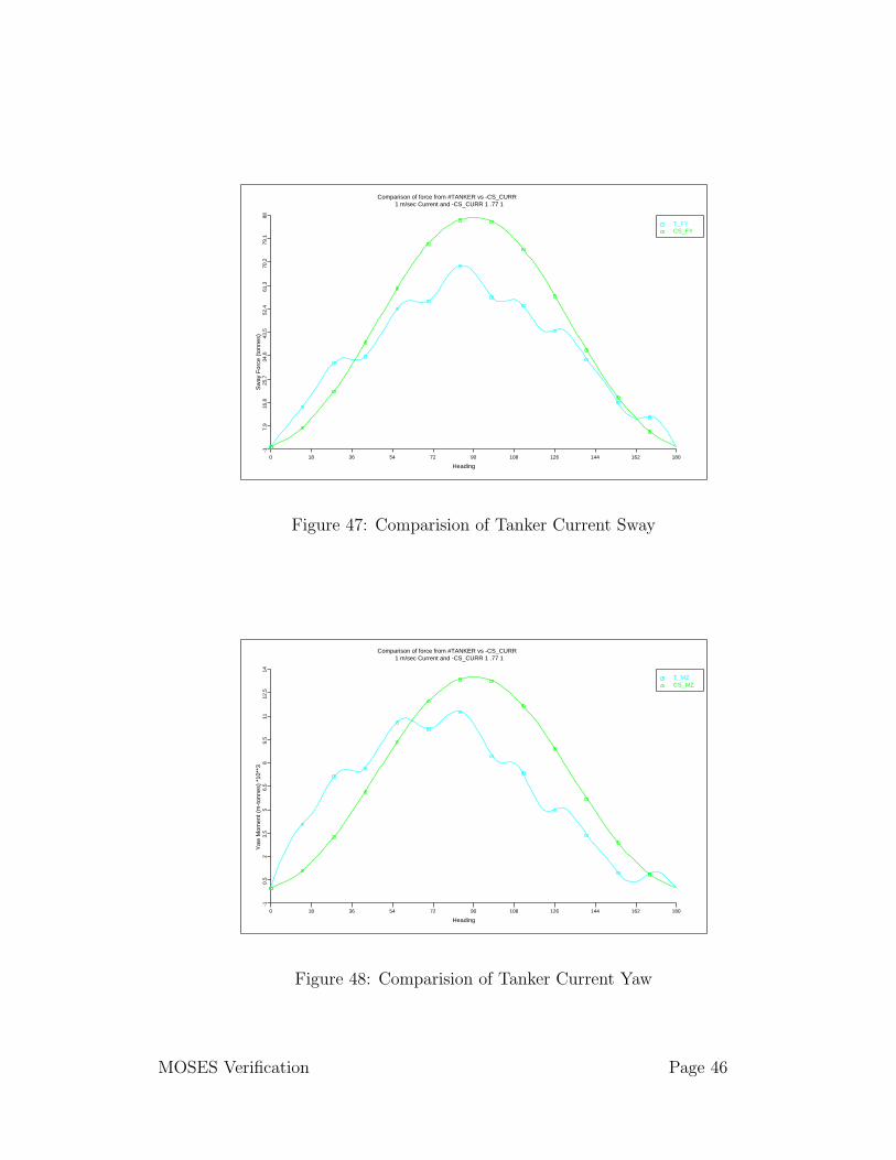
T_FYCS_FY
Comparison of force from #TANKER vs -CS_CURR1 m/sec Current and -CS_CURR 1 .77 1
0 18 36 54 72 90 108 126 144 162 180
Heading
-17.
916
.825
.734
.643
.552
.461
.370
.279
.188
Sw
ay F
orce
(to
nnes
)
Figure 47: Comparision of Tanker Current Sway
T_MZCS_MZ
Comparison of force from #TANKER vs -CS_CURR1 m/sec Current and -CS_CURR 1 .77 1
0 18 36 54 72 90 108 126 144 162 180
Heading
-10.
52
3.5
56.
58
9.5
1112
.514
Yaw
Mom
ent (
m-t
onne
s) *
10**
3
Figure 48: Comparision of Tanker Current Yaw
MOSES Verification Page 46

Figure 49 shows a comparison of the roll response of a barge for two values of wavesteepness (the same case considered in Section IX above). In one case, we have onlyTanaka damping while in the other we have only damping produced by the panelintegration method. The comparison here is remarkable. This is especially true sincethe ”Tanaka” damping is supposed to be a result of eddy formation at the bilge andthe panel integration is simply due to pressure drag over the bottom. This is quiteimportant. It says that if one uses panel integration to capture current force, thenhe should either set Cz to zero or set other roll damping to zero.
TANAKA, Steep=20CS 1 1 1, Steep=20TANAKA, Steep=75CS 1 1 1, Steep=75
Comparison of Roll RAO with TANAKA vs -CS_CURRUsing -CS_CURR 1 1 1
5 6.5 8 9.5 11 12.5 14 15.5 17 18.5 20
Period
00.
450.
91.
351.
82.
252.
73.
153.
64.
054.
5R
oll R
ao (
Deg
/Ft)
Figure 49: Comparision of Damping with TANAKA
Figure 50 and figure 51 show a comparison of the heave and roll response of theBALDER (same condition as that reported in Section X above) using #TUBE fordamping and using the panel integration method. Again, the agreement is excellentand the panel integration method does not require defining any ”special” elements.
Finally, figure 53 shows a comparison of the heave decay of the BALDER with com-puted panel integration damping, computed with 3% critical damping, and ModelTests. Again the comparison is quite good with the model tests showing more damp-ing than the other two methods.
MOSES Verification Page 47

HEAVE_#TUBEHEAVE_CS_CURR
Comparison of BALDER Beam Sea, Frequency ResponseSTEEPNESS 20 and -CS_CURR 1 1 1
3 5.9 8.8 11.7 14.6 17.5 20.4 23.3 26.2 29.1 32
Period
00.
330.
660.
991.
321.
651.
982.
312.
642.
973.
3H
eave
Rao
(M
/M)
Figure 50: Comparison of Damping with #TUBE in Heave
ROLL_#TUBEROLL_CS_CURR
Comparison of BALDER Beam Sea, Frequency ResponseSTEEPNESS 20 and -CS_CURR 1 1 1
3 5.9 8.8 11.7 14.6 17.5 20.4 23.3 26.2 29.1 32
Period
00.
140.
280.
420.
560.
70.
840.
981.
121.
261.
4R
oll R
ao (
Deg
/M )
Figure 51: Comparison of Damping with #TUBE in Roll
MOSES Verification Page 48

HEAVE_CS_CURRHEAVE_3%MODEL TEST HEAVE
Comparison of BALDER Decay using #TUBE vs -CS_CURR-CS_CURR 1 1 1
0 11 22 33 44 55 66 77 88 99 110
TIME
-2.5
-2.0
7-1
.64
-1.2
1-0
.78
-0.3
50.
080.
510.
941.
371.
8H
eave
Dec
ay (
M)
Figure 52: Heave Decay
MOSES Verification Page 49

XIV. PIPELAYING
In this section, we will consider the results of a static pipelaying analysis. In partic-ular, will will compare the results from MOSES to those of the OFFPIPE program.The pipe used here is a steel pipe, 12 inches diameter, 0.75 inch thickness, laid in 1600meters of waterdepth. The figure 53 shows both the axial force and bending momentalong the pipe resulting from each program. The two sets of curves agree well exceptfor the moment between 2800 meters and 2970 meters. This is probably due to thefact that OFFPIPE’s results used a nonlinear moment-curvature relationship whileMOSES used linear ones.
FIGURE 1
Offpipe AxialMOSES AxialOffpipe Bend MomMOSES Bend Mom
. .23 .46 .69 .92 1.15 1.38 1.61 1.84 2.07 2.3
Distance From Anchor, M *10**3
.26
.354
.448
.542
.636
.73
.824
.918
1.01
21.
106
1.2
Axi
al F
orce
, Kn
*10*
*3
.76
152
228
304
380
456
532
608
684
760
Ben
ding
Mom
, Kn-
M
Figure 53: Comparison of axial force and bending moment along the pipe
MOSES Verification Page 50

XV. QUALITY ASSURANCE PROCEDURES
There are two major factors which influence the applicability of a given piece ofsoftware: the validity of the initial program, and the care taken in its maintenance.When a new feature is added to the program, it is normally checked by exampleswhich can be verified by manual computations. The major question is how to assurethat during the maintenance process, something is not done to upset the initial resultswithin the proven range of validity. This section describes a set of procedures whichminimize the introduction of unintentional errors. One should notice that the goalof these procedures is to maintain a status quo in the results of the programs, not toinsure the applicability of the results to any given situation.
Company Structure
As a small scientific software vendor, Ultramarine has a corporate structure with theintegrity of its software as its basis. The corporate president has direct control ofevery step of the development, maintenance, and distribution of all software. Allof the personnel involved with these activities are graduate engineers with degreesin the area for which they develop software. Thus, each are allowed considerablediscretion in development and maintenance of our products. This freedom, however,is controlled by the Release Administrator who is responsible for the integrity of eachrelease of Ultramarine’s software. It is primarily the duties of this individual whichare discussed below.
Programming Standards
Research has shown that many errors can be eliminated by a set of programmingstandards, and that the particular ones adopted are not as important as the existenceof a standard. We have adopted most of the well accepted standards. While it isdifficult to quantify, we feel that the most important factor in software integrity isthe overall architecture of the product. To use currently popular jargon, systemsshould be designed “top down” and written with “structure”. The two elements ofour standard which we feel are next in importance are the typing of all variables andthe initialization of all data in only one location. The first of these, along with agood compiler, eliminates most of the typographical errors. The second mitigatesthe possibility of forgetting to change it in all places.
Corrective Action
To allow us flexibility in making major changes and enhancements we maintain twocomplete copies of all of our software. One copy is considered a “development” copy,while the second is a “release” copy. Major changes are made only in the develop-ment copy, and consequently the only changes made to the release copy are those
MOSES Verification Page 51

necessary to correct reported problems. The Release Administrator is responsible forresponding to all reported problems. If corrective action is necessary, the action isundertaken with his direction. It is his responsibility to document all changes in therelease copy of the software. This documentation includes:
1.) The discoverer of the problem,
2.) A description of the problem,
3.) The programs affected by the problem, and
4.) The changes in the code to fix the problem.
The revision number of all programs is incremented in the last digit whenever a changeis made in the release copy. Two types of verification are performed for problem fixes.The first is to execute a problem which exhibited the error to ascertain if the problemis, in fact, fixed. For most problems, this is all that is done. In some cases, however,the entire verification tests for a given program may be run to ensure that the fix hasno other impact.
New Versions
Whenever all of the major modifications have been made for a release, the devel-opment copy of the source is “migrated” to the release world. This migration isperformed by the Release Administrator. When a migration occurs, the revisionnumber is changed in the first digit past the decimal, or if the changes in a releaseare particularly dramatic, the number to the left of the decimal is incremented. Itis during this migration process that quality control procedures become increasinglyimportant, as one must be sure that all problems fixed in the previous release copywill be fixed in the new version.
The first step in this procedure is to archive a tape containing all of the data forthe old release. The next step is that the source of the current release is machinecompared with the original source of that release. Since any discrepancies betweenthese two sources should have been documented as a “problem fix”, the list of prob-lem fixes is compared to the true source changes to ensure that all alterations havebeen documented. Next, the source code of the new release version is compared, bymachine, with the source code of the previous version. The results of this compari-son are checked against the documented changes to make sure that all changes in theprevious release have been made in the new one. This machine comparison is thenarchived.
Verification
MOSES Verification Page 52

The final step in the migration procedure is to execute a set of standard verificationproblems. These verification data sets were designed to test each major option ofthe application, and currently there are a total of over one hundred problems whichcomprise the verification suite. The results of the verification runs are compared, bymachine, with the results of the same test executed on the previous release. Anydifferences in the results are justified considering the changes in the release, and thecomparison of the results is filed for reference. After any discrepancies between theresults of the verification runs have been resolved, the process repeats.
Documentation
The documentation for each application is maintained in a manner similar to thesource code. At the end of a release cycle, the documentation is revised so that itaccurately reflects the new version of the program. After the manuals have beenrevised, a copy of each one is proofread, and any errors are corrected. The manualsare then printed for the release. Since the only changes which can be made during arelease cycle are to fix errors, a set of documentation is valid for any version of theprogram which has the same revision numbers to the left of the decimal, and for thefirst digit to the right of the decimal. The revision number for the documentation isprinted on the bottom of each page of the documentation.
Releases
Our software is actually supplied to a site on a “release tape”, the format of whichvaries with the type of computer at the site. In fact, for some installations, the releasewill be supplied on a media other than tape. Each tape will contain:
1.) All of the modules necessary to install the programs at the site,
2.) A new manual for each program on the tape, and
3.) Our verification data sets for each program on the tape.
Along with the tape, a document describing the changes made in this release isenclosed. The actual process of writing release tapes has been automated. One ofour products, URSULA, keeps a database of which customers have which programs,and when instructed, a tape tailored for that site will be written. URSULA alsokeeps a database of the date the tape was sent and the revision number of the productson the tape.
MOSES Verification Page 53

References
[1] Barge Motions Research Project, Phase 1 Report, for a consortium of companiesorganised by Noble Denton and Associates Ltd., December 1978.
[2] Prediction of Wind and Current Loads on VLCCs by the Oil Companies Inter-national Forum (OCIMF).
[3] Netherlands Ship Model Basin Report No. 45065-1-ZT, The Damping ControlledResponse of Semi-submersibles Wageningen, February, 1984.
[4] Wichers, J.E.W., ”The Prediction of the Behaviour of Single Point MooredTankers”, Floating Structures and Offshore Operation , Elsevier Place, Oxford,1988.
MOSES Verification Page 54