verification problems : 15 : drained and undrained ...web.mst.edu/~norbert/ge5471/assignments/assign...

Drained and Undrained Triaxial Compression Test on a Cam-Clay Sample 15 - 1

15 Drained and Undrained Triaxial Compression Test on a Cam-Clay Sample

15.1 Problem Statement

Conventional drained and undrained triaxial compression tests on Cam-clay soil samples are mod-eled using FLAC. The stresses and specific volume at the critical state are compared with ana-lytical predictions. The responses of both a lightly over-consolidated (LOC) and a heavily over-consolidated (HOC) specimen are considered. This set of problems tests the prediction accuracyof the modified Cam-clay model in FLAC.

The model of the sample is a cylinder with unit height and circular cross-section with unit radius.The sample is made of a Cam-clay material with the following properties:

shear modulus (G) 250 × p′1

soil constant (M) 1.02

slope of normal consolidation line (λ) 0.2

slope of elastic swelling line (κ) 0.05

reference pressure (p′1) 1 kPa

pre-consolidation pressure (p′c0):

lightly over-consolidated 8 × p′1

heavily over-consolidated 40 × p′1

specific volume at reference pressure

on normal consolidation line, (vλ) 3.32

density (ρ) 1000 kg / m3

Initially, the sample is in a state of isotropic compression corresponding to p0 = 5p′1 and zero

excess pore pressure (p′0 = p0). The pre-consolidation pressure, p′

c0, has magnitude 8 × p′1 in

the lightly over-consolidated case, and 40 × p′1 in the heavily over-consolidated case. These cases

correspond to an over-consolidation ratio, R = p′c0/p

′0, of 1.6 and 8, respectively. The shear

modulus is assumed to remain constant during the test carried out with constant confining pressure,p0, and simulated strain-controlled platens. Drained and undrained tests are considered. Refer toWood (1990) for a detailed discussion on the Cam-clay plasticity theory.

FLAC Version 6.0

15 - 2 Verification Problems

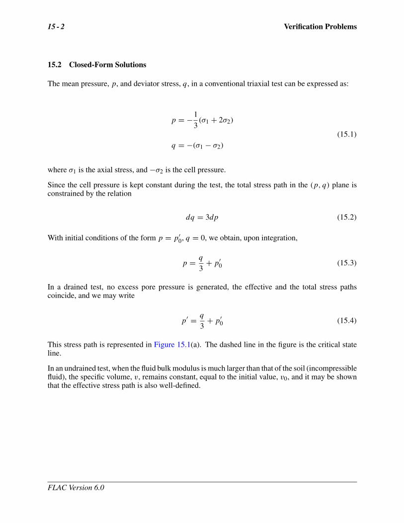
15.2 Closed-Form Solutions

The mean pressure, p, and deviator stress, q, in a conventional triaxial test can be expressed as:

p = −1

3(σ1 + 2σ2)

(15.1)

q = −(σ1 − σ2)

where σ1 is the axial stress, and −σ2 is the cell pressure.

Since the cell pressure is kept constant during the test, the total stress path in the (p, q) plane isconstrained by the relation

dq = 3dp (15.2)

With initial conditions of the form p = p′0, q = 0, we obtain, upon integration,

p = q

3+ p′

0 (15.3)

In a drained test, no excess pore pressure is generated, the effective and the total stress pathscoincide, and we may write

p′ = q

3+ p′

0 (15.4)

This stress path is represented in Figure 15.1(a). The dashed line in the figure is the critical stateline.

In an undrained test, when the fluid bulk modulus is much larger than that of the soil (incompressiblefluid), the specific volume, v, remains constant, equal to the initial value, v0, and it may be shownthat the effective stress path is also well-defined.

FLAC Version 6.0


p'0 p'0 p'c0 p'

qq=Mp'

criticalpoint

criticalpoint

LOCHOC

a. drained

p'0 p'0 p'c0 p'

q

q=Mp'

criticalpoints

LOCHOC

I

b. undrained

I

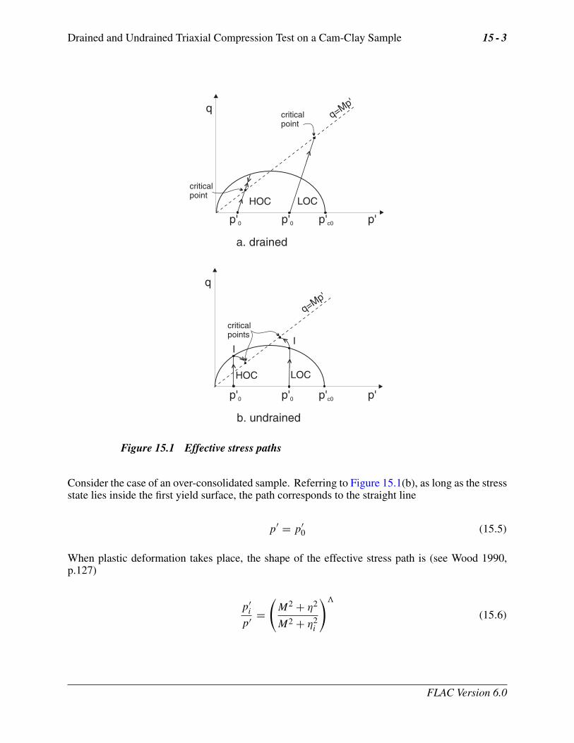
Figure 15.1 Effective stress paths

Consider the case of an over-consolidated sample. Referring to Figure 15.1(b), as long as the stressstate lies inside the first yield surface, the path corresponds to the straight line

p′ = p′0 (15.5)

When plastic deformation takes place, the shape of the effective stress path is (see Wood 1990,p.127)

p′i

p′ =(

M2 + η2

M2 + η2i

)�

(15.6)

FLAC Version 6.0


where � = (λ − κ)/λ, η = q/p′ and p′i and ηi define the effective stress state at impending yield,

indicated as point I in Figure 15.1(b).

Note that, under undrained conditions, the yield path is defined by an equation of the form shownin Eq. (15.6) for any boundary condition (i.e., not only under triaxial compression conditions).

Intersection of the yield curve through p′c0 with the straight path p′ = p′

0, gives (using thatR = p′

c0/p′0):

p′i = p′

0

(15.7)

η2i = M2(R − 1)

After substitution of those expressions in Eq. (15.6), we obtain

p′0

p′ =(

M2 + η2

M2R

)�

(15.8)

p'cr ln(p' )cr2p'cr ln (2p' )crp' ln p'

qcr

vcr

q v

q=Mp'

plasticvolumetriccompression

swellingline

plasticvolumetricdilation

normalconsolidationline

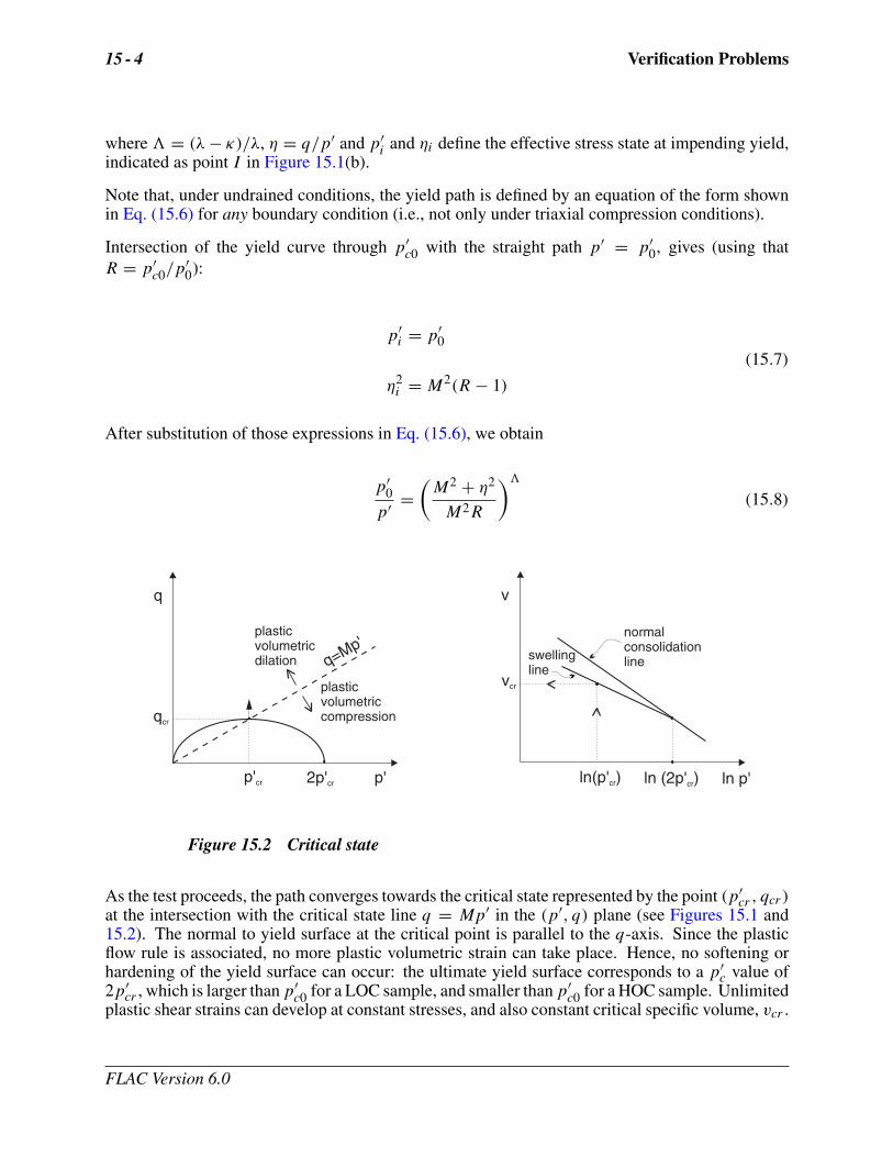
Figure 15.2 Critical state

As the test proceeds, the path converges towards the critical state represented by the point (p′cr , qcr )

at the intersection with the critical state line q = Mp′ in the (p′, q) plane (see Figures 15.1 and15.2). The normal to yield surface at the critical point is parallel to the q-axis. Since the plasticflow rule is associated, no more plastic volumetric strain can take place. Hence, no softening orhardening of the yield surface can occur: the ultimate yield surface corresponds to a p′

c value of2p′

cr , which is larger than p′c0 for a LOC sample, and smaller than p′

c0 for a HOC sample. Unlimitedplastic shear strains can develop at constant stresses, and also constant critical specific volume, vcr .

FLAC Version 6.0


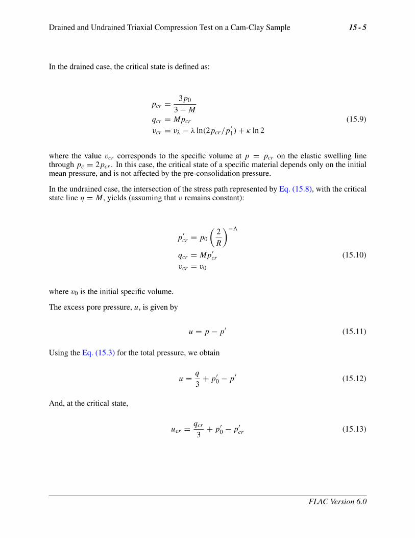
In the drained case, the critical state is defined as:

pcr = 3p0

3 − M

qcr = Mpcr (15.9)

vcr = vλ − λ ln(2pcr/p′1) + κ ln 2

where the value vcr corresponds to the specific volume at p = pcr on the elastic swelling linethrough pc = 2pcr . In this case, the critical state of a specific material depends only on the initialmean pressure, and is not affected by the pre-consolidation pressure.

In the undrained case, the intersection of the stress path represented by Eq. (15.8), with the criticalstate line η = M , yields (assuming that v remains constant):

p′cr = p0

(2

R

)−�

qcr = Mp′cr (15.10)

vcr = v0

where v0 is the initial specific volume.

The excess pore pressure, u, is given by

u = p − p′ (15.11)

Using the Eq. (15.3) for the total pressure, we obtain

u = q

3+ p′

0 − p′ (15.12)

And, at the critical state,

ucr = qcr

3+ p′

0 − p′cr (15.13)

FLAC Version 6.0


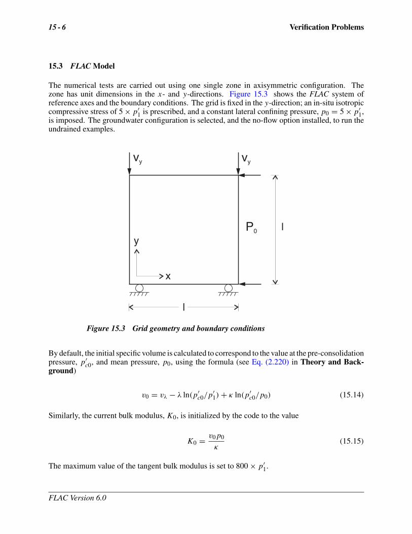
15.3 FLAC Model

The numerical tests are carried out using one single zone in axisymmetric configuration. Thezone has unit dimensions in the x- and y-directions. Figure 15.3 shows the FLAC system ofreference axes and the boundary conditions. The grid is fixed in the y-direction; an in-situ isotropiccompressive stress of 5 × p′

1 is prescribed, and a constant lateral confining pressure, p0 = 5 × p′1,

is imposed. The groundwater configuration is selected, and the no-flow option installed, to run theundrained examples.

yP0

vy vy

x

l

l

Figure 15.3 Grid geometry and boundary conditions

By default, the initial specific volume is calculated to correspond to the value at the pre-consolidationpressure, p′

c0, and mean pressure, p0, using the formula (see Eq. (2.220) in Theory and Back-ground)

v0 = vλ − λ ln(p′c0/p

′1) + κ ln(p′

c0/p0) (15.14)

Similarly, the current bulk modulus, K0, is initialized by the code to the value

K0 = v0p0

κ(15.15)

The maximum value of the tangent bulk modulus is set to 800 × p′1.

FLAC Version 6.0


A compressive velocity is applied in cycles of 40 steps at the top of the model: the velocity magnitudeis set to a finite value for the first 20 steps, and to zero for the remaining part of the cycle. A total of5,000 cycles with a velocity magnitude of 0.5 × 10−4 m/sec was used in the drained examples. Forthe undrained tests, the porosity, n, is derived from the specific volume using n = (v−1)/v, and thewater bulk modulus is set to 2 × 104 ×p′

1 (a large value compared to the initial value of the productnK , which is of the order 102 × p′

1). In this case, a compressive velocity of magnitude 0.5 × 10−6

m/sec is applied for a total of 10,000 cycles. The mean pressure, deviator stress, specific volumeand, in the undrained case, pore pressure are monitored as they converge to the critical state.

The data file “CAM.DAT” in Section 15.6 was used to carry out the drained and undrained numericaltests. The property mpc was adjusted there to the values 8 and 40, to treat the lightly and heavilyover-consolidated cases, respectively. FISH functions are used to apply the velocity boundaryconditions and evaluate the relative error made at the end of the simulation.

15.4 FLAC Results and Discussion

Numerical values for p, q and v for the drained case, and p′1, q, v and u for the undrained case, are

compared with the analytical predictions at the end of each simulation. The results, presented inTables 15.1 and 15.2, indicate relative errors of less than 2%.

Table 15.1 Drained case

R = 1.6 R = 8 Analytical

p 7.590 7.600 7.576q 7.779 7.818 7.727v 2.810 2.809 2.811

Table 15.2 Undrained case

R = 1.6 R = 8Numerical Analytical Numerical Analytical

p′1 4.239 4.229 1.407 × 101 1.414 × 101

q 4.317 4.314 1.442 × 101 1.442 × 101

v 2.927 2.928 2.687 2.686u 2.201 2.209 −4.258 −4.334

FLAC Version 6.0


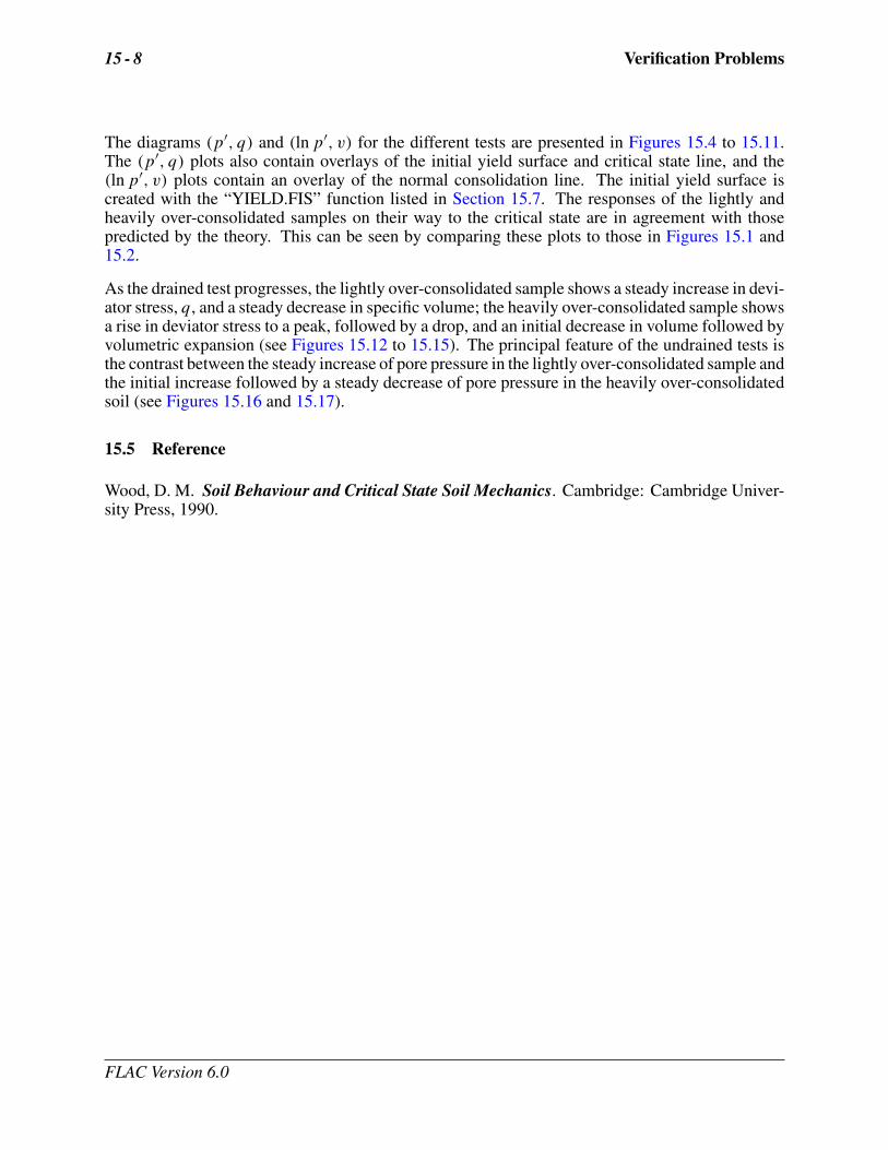
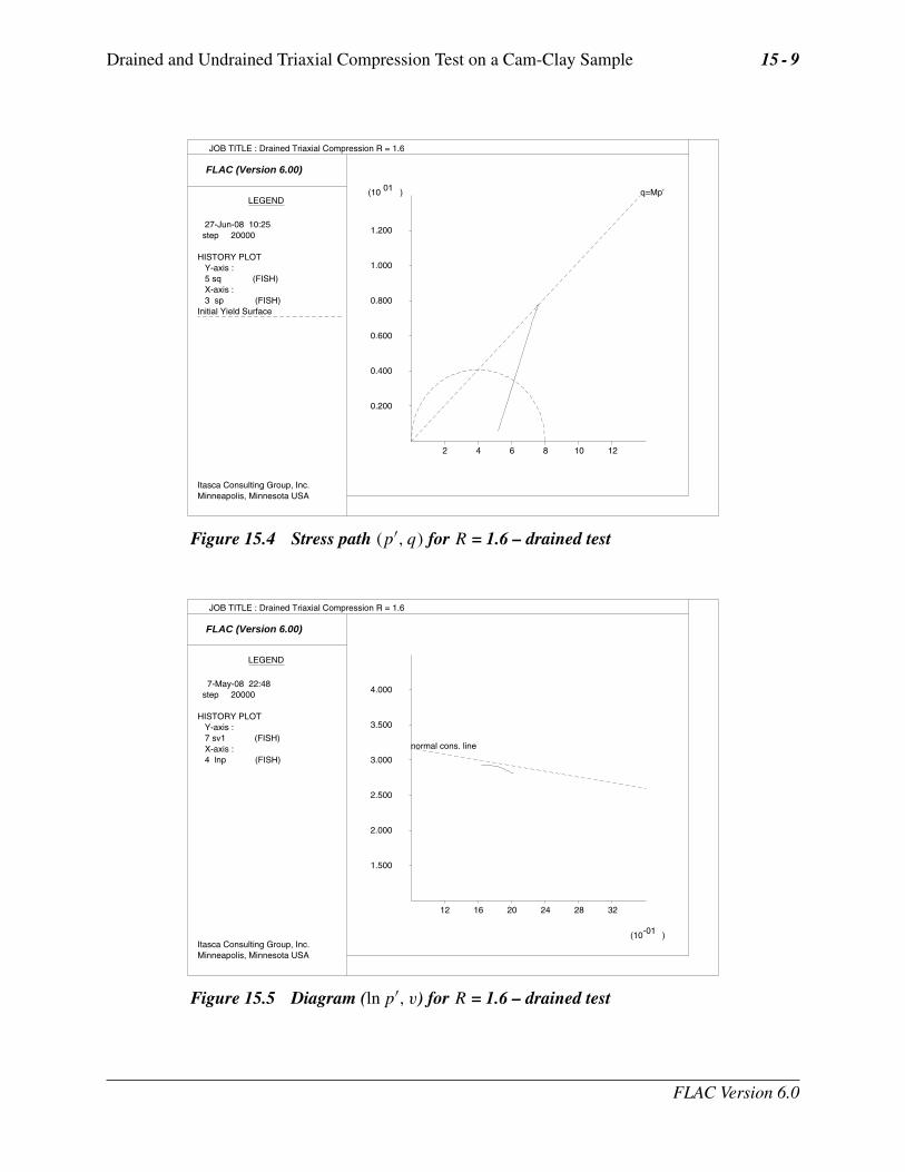
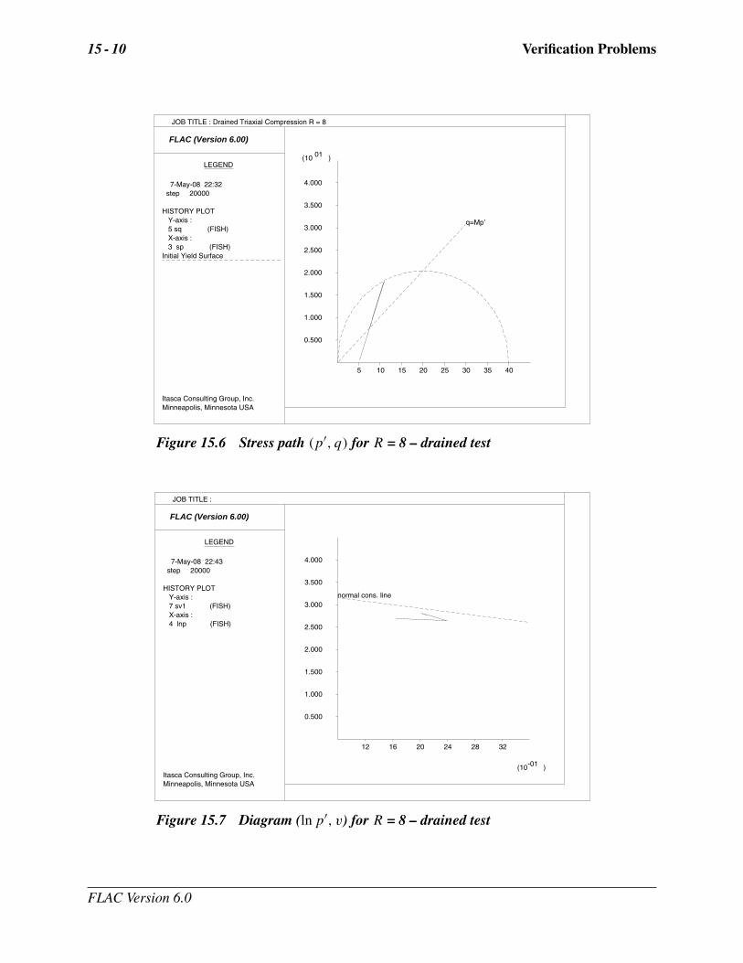
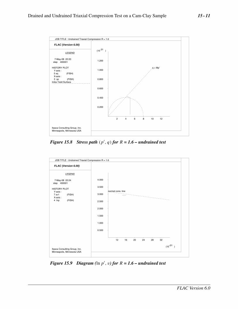
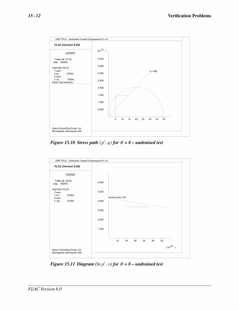
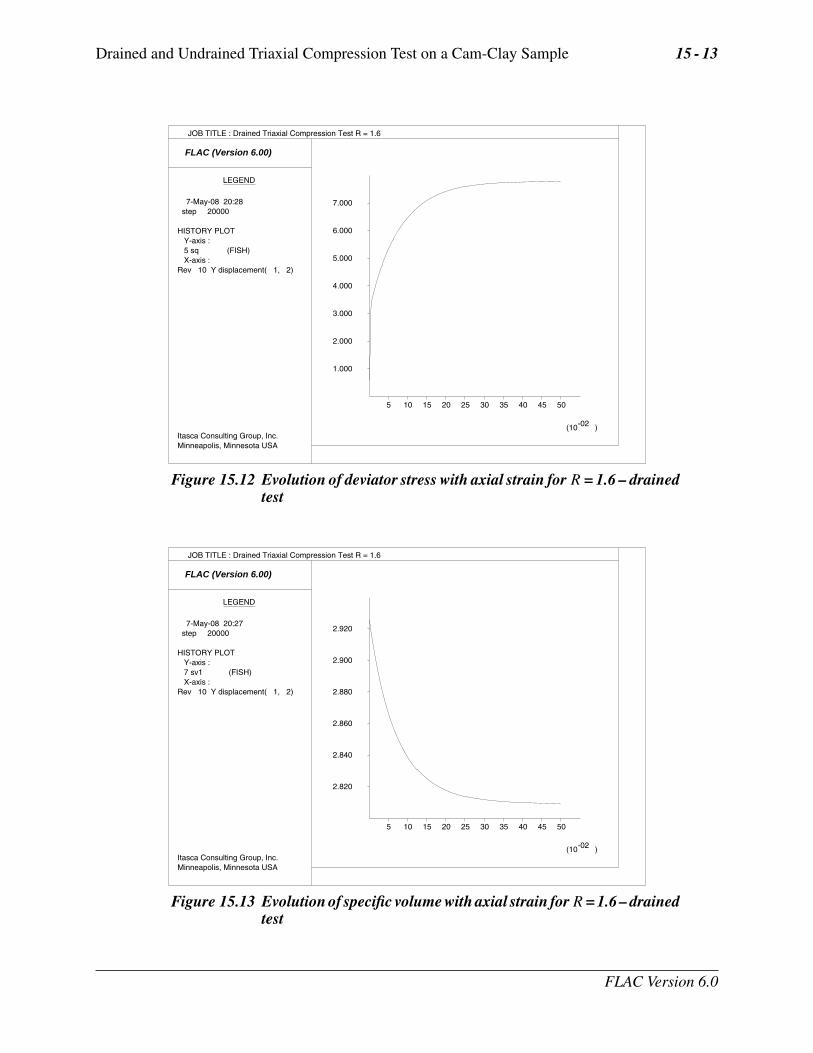
The diagrams (p′, q) and (ln p′, v) for the different tests are presented in Figures 15.4 to 15.11.The (p′, q) plots also contain overlays of the initial yield surface and critical state line, and the(ln p′, v) plots contain an overlay of the normal consolidation line. The initial yield surface iscreated with the “YIELD.FIS” function listed in Section 15.7. The responses of the lightly andheavily over-consolidated samples on their way to the critical state are in agreement with thosepredicted by the theory. This can be seen by comparing these plots to those in Figures 15.1 and15.2.

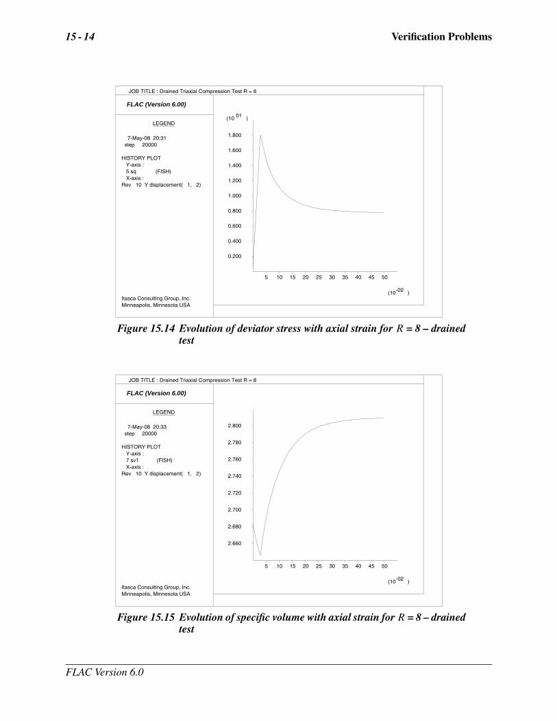
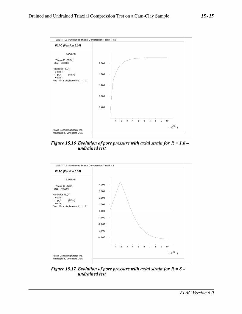
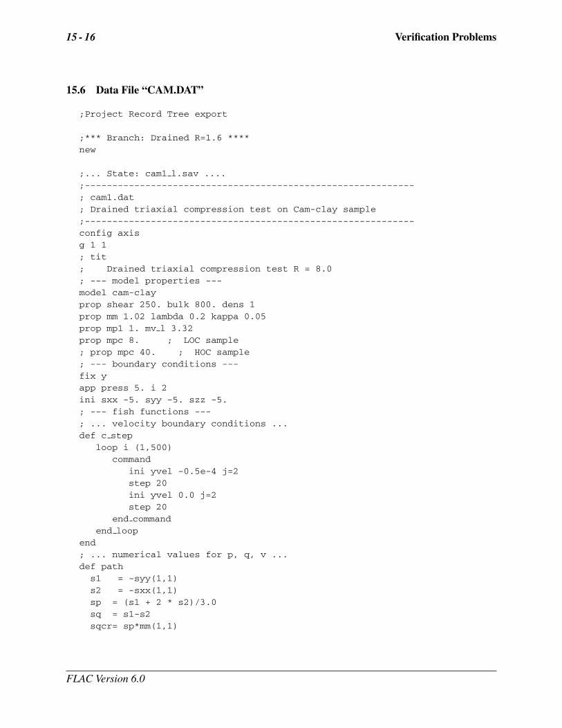
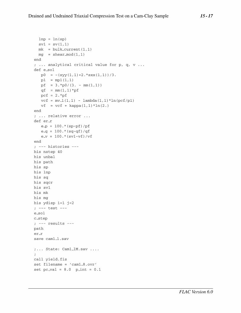
As the drained test progresses, the lightly over-consolidated sample shows a steady increase in devi-ator stress, q, and a steady decrease in specific volume; the heavily over-consolidated sample showsa rise in deviator stress to a peak, followed by a drop, and an initial decrease in volume followed byvolumetric expansion (see Figures 15.12 to 15.15). The principal feature of the undrained tests isthe contrast between the steady increase of pore pressure in the lightly over-consolidated sample andthe initial increase followed by a steady decrease of pore pressure in the heavily over-consolidatedsoil (see Figures 15.16 and 15.17).

15.5 Reference

Wood, D. M. Soil Behaviour and Critical State Soil Mechanics. Cambridge: Cambridge Univer-sity Press, 1990.

FLAC Version 6.0


FLAC (Version 6.00)

LEGEND

27-Jun-08 10:25 step 20000 HISTORY PLOT Y-axis : 5 sq (FISH) X-axis : 3 sp (FISH)

2 4 6 8 10 12

0.200

0.400

0.600

0.800

1.000

1.200

(10 ) 01

Initial Yield Surface

q=Mp’

JOB TITLE : Drained Triaxial Compression R = 1.6

Itasca Consulting Group, Inc. Minneapolis, Minnesota USA

Figure 15.4 Stress path (p′, q) for R = 1.6 – drained test

FLAC (Version 6.00)

LEGEND

7-May-08 22:48 step 20000 HISTORY PLOT Y-axis : 7 sv1 (FISH) X-axis : 4 lnp (FISH)

12 16 20 24 28 32

(10 )-01

1.500

2.000

2.500

3.000

3.500

4.000

normal cons. line

JOB TITLE : Drained Triaxial Compression R = 1.6


Figure 15.5 Diagram (ln p′, v) for R = 1.6 – drained test

FLAC Version 6.0


FLAC (Version 6.00)

LEGEND

7-May-08 22:32 step 20000 HISTORY PLOT Y-axis : 5 sq (FISH) X-axis : 3 sp (FISH)

5 10 15 20 25 30 35 40

0.500

1.000

1.500

2.000

2.500

3.000

3.500

4.000

(10 ) 01

Initial Yield Surface

q=Mp’

JOB TITLE : Drained Triaxial Compression R = 8


Figure 15.6 Stress path (p′, q) for R = 8 – drained test

FLAC (Version 6.00)

LEGEND


12 16 20 24 28 32

(10 )-01

0.500

1.000

1.500

2.000

2.500

3.000

3.500

4.000

normal cons. line

JOB TITLE :


Figure 15.7 Diagram (ln p′, v) for R = 8 – drained test

FLAC Version 6.0


FLAC (Version 6.00)

LEGEND


2 4 6 8 10 12

0.200

0.400

0.600

0.800

1.000

1.200

(10 ) 01

Initia Yield Surface

q = Mp’

JOB TITLE : Undrained Triaxial Compression R = 1.6


Figure 15.8 Stress path (p′, q) for R = 1.6 – undrained test

FLAC (Version 6.00)

LEGEND


12 16 20 24 28 32

(10 )-01

0.500

1.000

1.500

2.000

2.500

3.000

3.500

4.000

normal cons. line

JOB TITLE : Undrained Triaxial Compression R = 1.6


Figure 15.9 Diagram (ln p′, v) for R = 1.6 – undrained test

FLAC Version 6.0


FLAC (Version 6.00)

LEGEND


5 10 15 20 25 30 35 40

0.500

1.000

1.500

2.000

2.500

3.000

3.500

4.000

(10 ) 01

Initial Yield Interface

q = Mp’

JOB TITLE : Undrained Triaxial Compression R = 8


Figure 15.10 Stress path (p′, q) for R = 8 – undrained test

FLAC (Version 6.00)

LEGEND


12 16 20 24 28 32

(10 )-01

1.500

2.000

2.500

3.000

3.500

4.000

normal cons. line

JOB TITLE : Undrained Triaxial Compression R = 8


Figure 15.11 Diagram (ln p′, v) for R = 8 – undrained test

FLAC Version 6.0


FLAC (Version 6.00)

LEGEND

7-May-08 20:28 step 20000 HISTORY PLOT Y-axis : 5 sq (FISH) X-axis :Rev 10 Y displacement( 1, 2)

5 10 15 20 25 30 35 40 45 50

(10 )-02

1.000

2.000

3.000

4.000

5.000

6.000

7.000

JOB TITLE : Drained Triaxial Compression Test R = 1.6


Figure 15.12 Evolution of deviator stress with axial strain for R = 1.6 – drainedtest

FLAC (Version 6.00)

LEGEND

7-May-08 20:27 step 20000 HISTORY PLOT Y-axis : 7 sv1 (FISH) X-axis :Rev 10 Y displacement( 1, 2)

5 10 15 20 25 30 35 40 45 50

(10 )-02

2.820

2.840

2.860

2.880

2.900

2.920

JOB TITLE : Drained Triaxial Compression Test R = 1.6


Figure 15.13 Evolution of specific volume with axial strain forR = 1.6 – drainedtest

FLAC Version 6.0


FLAC (Version 6.00)

LEGEND

7-May-08 20:31 step 20000 HISTORY PLOT Y-axis : 5 sq (FISH) X-axis :Rev 10 Y displacement( 1, 2)

5 10 15 20 25 30 35 40 45 50

(10 )-02

0.200

0.400

0.600

0.800

1.000

1.200

1.400

1.600

1.800

(10 ) 01

JOB TITLE : Drained Triaxial Compression Test R = 8


Figure 15.14 Evolution of deviator stress with axial strain for R = 8 – drainedtest

FLAC (Version 6.00)

LEGEND

7-May-08 20:33 step 20000 HISTORY PLOT Y-axis : 7 sv1 (FISH) X-axis :Rev 10 Y displacement( 1, 2)

5 10 15 20 25 30 35 40 45 50

(10 )-02

2.660

2.680

2.700

2.720

2.740

2.760

2.780

2.800

JOB TITLE : Drained Triaxial Compression Test R = 8


Figure 15.15 Evolution of specific volume with axial strain for R = 8 – drainedtest

FLAC Version 6.0


FLAC (Version 6.00)

LEGEND

7-May-08 20:34 step 400001 HISTORY PLOT Y-axis : 11 p_fl (FISH) X-axis :Rev 10 Y displacement( 1, 2)

1 2 3 4 5 6 7 8 9 10

(10 )-02

0.400

0.800

1.200

1.600

2.000

JOB TITLE : Undrained Triaxial Compression Test R = 1.6


Figure 15.16 Evolution of pore pressure with axial strain for R = 1.6 –undrained test

FLAC (Version 6.00)

LEGEND

7-May-08 20:34 step 400001 HISTORY PLOT Y-axis : 11 p_fl (FISH) X-axis :Rev 10 Y displacement( 1, 2)

1 2 3 4 5 6 7 8 9 10

(10 )-02

-4.000

-3.000

-2.000

-1.000

0.000

1.000

2.000

3.000

4.000

JOB TITLE : Undrained Triaxial Compression Test R = 8


Figure 15.17 Evolution of pore pressure with axial strain for R = 8 –undrained test

FLAC Version 6.0


15.6 Data File “CAM.DAT”

;Project Record Tree export

;*** Branch: Drained R=1.6 ****new

;... State: cam1 l.sav ....;------------------------------------------------------------; cam1.dat; Drained triaxial compression test on Cam-clay sample;------------------------------------------------------------config axisg 1 1; tit; Drained triaxial compression test R = 8.0; --- model properties ---model cam-clayprop shear 250. bulk 800. dens 1prop mm 1.02 lambda 0.2 kappa 0.05prop mp1 1. mv l 3.32prop mpc 8. ; LOC sample; prop mpc 40. ; HOC sample; --- boundary conditions ---fix yapp press 5. i 2ini sxx -5. syy -5. szz -5.; --- fish functions ---; ... velocity boundary conditions ...def c step

loop i (1,500)command

ini yvel -0.5e-4 j=2step 20ini yvel 0.0 j=2step 20

end commandend loop

end; ... numerical values for p, q, v ...def path

s1 = -syy(1,1)s2 = -sxx(1,1)sp = (s1 + 2 * s2)/3.0sq = s1-s2sqcr= sp*mm(1,1)

FLAC Version 6.0


lnp = ln(sp)sv1 = sv(1,1)mk = bulk current(1,1)mg = shear mod(1,1)

end; ... analytical critical value for p, q, v ...def e sol

p0 = -(syy(1,1)+2.*sxx(1,1))/3.p1 = mp1(1,1)pf = 3.*p0/(3. - mm(1,1))qf = mm(1,1)*pfpcf = 2.*pfvcf = mv l(1,1) - lambda(1,1)*ln(pcf/p1)vf = vcf + kappa(1,1)*ln(2.)

end; ... relative error ...def er r

e p = 100.*(sp-pf)/pfe q = 100.*(sq-qf)/qfe v = 100.*(sv1-vf)/vf

end; --- histories ---his nstep 40his unbalhis pathhis sphis lnphis sqhis sqcrhis sv1his mkhis mghis ydisp i=1 j=2; --- test ---e solc step; --- results ---pather rsave cam1 l.sav

;... State: Cam1 lM.sav ....;call yield.fisset filename = ’cam1 8.ovr’set pc val = 8.0 p int = 0.1

FLAC Version 6.0


set m val = 1.02 p num = 81yield surface;save Cam1 lM.sav

;*** Branch: Drained R=8 ****new

;... State: cam1 h.sav ....;------------------------------------------------------------; cam1.dat; Drained triaxial compression test on Cam-clay sample;------------------------------------------------------------config axisg 1 1;tit; Drained triaxial compression test R = 1.6

; --- model properties ---model cam-clayprop shear 250. bulk 800. dens 1prop mm 1.02 lambda 0.2 kappa 0.05prop mp1 1. mv l 3.32;prop mpc 8. ; LOC sampleprop mpc 40. ; HOC sample; --- boundary conditions ---fix yapp press 5. i 2ini sxx -5. syy -5. szz -5.; --- fish functions ---; ... velocity boundary conditions ...def c step



end commandend loop


s1 = -syy(1,1)s2 = -sxx(1,1)sp = (s1 + 2 * s2)/3.0sq = s1-s2

FLAC Version 6.0


sqcr= sp*mm(1,1)lnp = ln(sp)sv1 = sv(1,1)mk = bulk current(1,1)mg = shear mod(1,1)


p0 = -(syy(1,1)+2.*sxx(1,1))/3.p1 = mp1(1,1)pf = 3.*p0/(3. - mm(1,1))qf = mm(1,1)*pfpcf = 2.*pfvcf = mv l(1,1) - lambda(1,1)*ln(pcf/p1)vf = vcf + kappa(1,1)*ln(2.)


e p = 100.*(sp-pf)/pfe q = 100.*(sq-qf)/qfe v = 100.*(sv1-vf)/vf

end; --- histories ---his nstep 40his unbalhis pathhis sphis lnphis sqhis sqcrhis sv1his mkhis mghis ydisp i=1 j=2; --- test ---e solc step; --- results ---path

er r;save cam1 l.savsave cam1 h.sav

;... State: Cam1 hM.sav ....;call yield.fis

FLAC Version 6.0


set filename = ’cam1 40.ovr’set pc val = 40.0 p int = 0.5set m val = 1.02 p num = 81yield surface;save Cam1 hM.sav

;*** Branch: Undrained R=1.6 ****new

;... State: cam2 l.sav ....config axis gwg 1 1; tit; Undrained triaxial compression test R = 1.6; --- model properties ---model cam-clayprop shear 250. bulk 800. dens 1prop mm 1.02 lambda 0.2 kappa 0.05prop mp1 1. mv l 3.32prop mpc 8.0 ; LOC sample; prop mpc 40.0 ; HOC samplewater bulk 2.e4 ten 1e10; --- boundary conditions ---fix yapp press 5. i 2ini sxx -5. syy -5. szz -5.set flow off; --- fish functions ---; ... initial specific volume, tangent bulk modulus, porosity ...def set n0

v0 = mv0(1,1) ; not available before cyclingn0 = (v0 - 1.) / v0command

prop por n0end command

end; ... velocity boundary conditions ...; ... velocity boundary conditions ...def c step



FLAC Version 6.0


end commandend loop


s1 = -syy(1,1)s2 = -sxx(1,1)p fl = pp(1,1)sp = (s1 + 2. * s2)/3.0 - p flsq = s1-s2sqcr= sp*mm(1,1)lnp = ln(sp)sv1 = sv(1,1)mk = bulk current(1,1)mg = shear mod(1,1)


p0 = -(syy(1,1) + 2. * sxx(1,1)) / 3.rr = mpc(1,1) / p0mbl = -1. + kappa(1,1) / lambda(1,1)aux = mbl * ln(2./rr)pf = p0 * exp(aux)pcf1 = pf*2.qf = mm(1,1)*pfpfl = qf/3. + p0 - pfvf = mv0(1,1)


e p = 100.*(sp-pf)/pfe q = 100.*(sq-qf)/qfe v = 100.*(sv1-vf)/vfe pf= 100.*(p fl-pfl)/pfl

end; --- histories ---his nstep 2000his unbalhis pathhis sphis lnphis sqhis sqcrhis sv1his mkhis mg

FLAC Version 6.0


his ydisp i=1 j=2his p fl; --- test ---step 1set n0e solc steppather rsave cam2 l.sav

;... State: Cam2 lM.sav ....call yield.fisset filename = ’cam2 8.ovr’set pc val = 8.0 p int = 0.1set m val = 1.02 p num = 81yield surfacesave Cam2 lM.sav

;*** Branch: Undrained R=8 ****new

;... State: cam2 h.sav ....config axis gwg 1 1;tit; Undrained triaxial compression test R = 1.6

; --- model properties ---model cam-clayprop shear 250. bulk 800. dens 1prop mm 1.02 lambda 0.2 kappa 0.05prop mp1 1. mv l 3.32;prop mpc 8.0 ; LOC sampleprop mpc 40.0 ; HOC samplewater bulk 2.e4 ten 1e10; --- boundary conditions ---fix yapp press 5. i 2ini sxx -5. syy -5. szz -5.set flow off; --- fish functions ---; ... initial specific volume, tangent bulk modulus, porosity ...def set n0

v0 = mv0(1,1) ; not available before cyclingn0 = (v0 - 1.) / v0command

FLAC Version 6.0


prop por n0end command

end; ... velocity boundary conditions ...def c step



end commandend loop


s1 = -syy(1,1)s2 = -sxx(1,1)p fl = pp(1,1)sp = (s1 + 2. * s2)/3.0 - p flsq = s1-s2sqcr= sp*mm(1,1)lnp = ln(sp)sv1 = sv(1,1)mk = bulk current(1,1)mg = shear mod(1,1)


p0 = -(syy(1,1) + 2. * sxx(1,1)) / 3.rr = mpc(1,1) / p0mbl = -1. + kappa(1,1) / lambda(1,1)aux = mbl * ln(2./rr)pf = p0 * exp(aux)pcf1 = pf*2.qf = mm(1,1)*pfpfl = qf/3. + p0 - pfvf = mv0(1,1)


e p = 100.*(sp-pf)/pfe q = 100.*(sq-qf)/qfe v = 100.*(sv1-vf)/vfe pf= 100.*(p fl-pfl)/pfl

end

FLAC Version 6.0


; --- histories ---his nstep 2000his unbalhis pathhis sphis lnphis sqhis sqcrhis sv1his mkhis mghis ydisp i=1 j=2his p fl; --- test ---step 1set n0e solc steppather r; save cam2 l.savsave cam2 h.sav

;... State: Cam2 hM.sav ....call yield.fisset filename = ’cam2 40.ovr’set pc val = 40.0 p int = 0.5set m val = 1.02 p num = 81yield surfacesave Cam2 hM.sav

;*** plot commands ****;plot name: Stress path R=8label arrow 1 (30.0,30.69) (0.0,0.0)q=Mp’set overlay file cam2 40.ovrplot hold history 5 line vs 3 overlay red alias ’Initial Yield Interface’&label 1 red

;plot name: Diagram (ln p’, v)label arrow 1 (0.0,3.32) (11.6,1.0)normal cons. lineplot hold history 7 line vs 4 label 1 red label 1 red;plot name: Evolution of deviator stressplot hold history 5 line vs -10;plot name: Evolution of specific volumeplot hold history 7 line vs -10

FLAC Version 6.0


;plot name: Evolution of pore pressureplot hold history 11 line vs -10;plot name: Stress path R=1.6label arrow 1 (10.0,10.32) (0.0,0.0)q = Mp’set overlay file cam1 8.ovrplot hold history 5 line vs 3 overlay red alias ’Initial Yield Surface’&label 1 red

FLAC Version 6.0


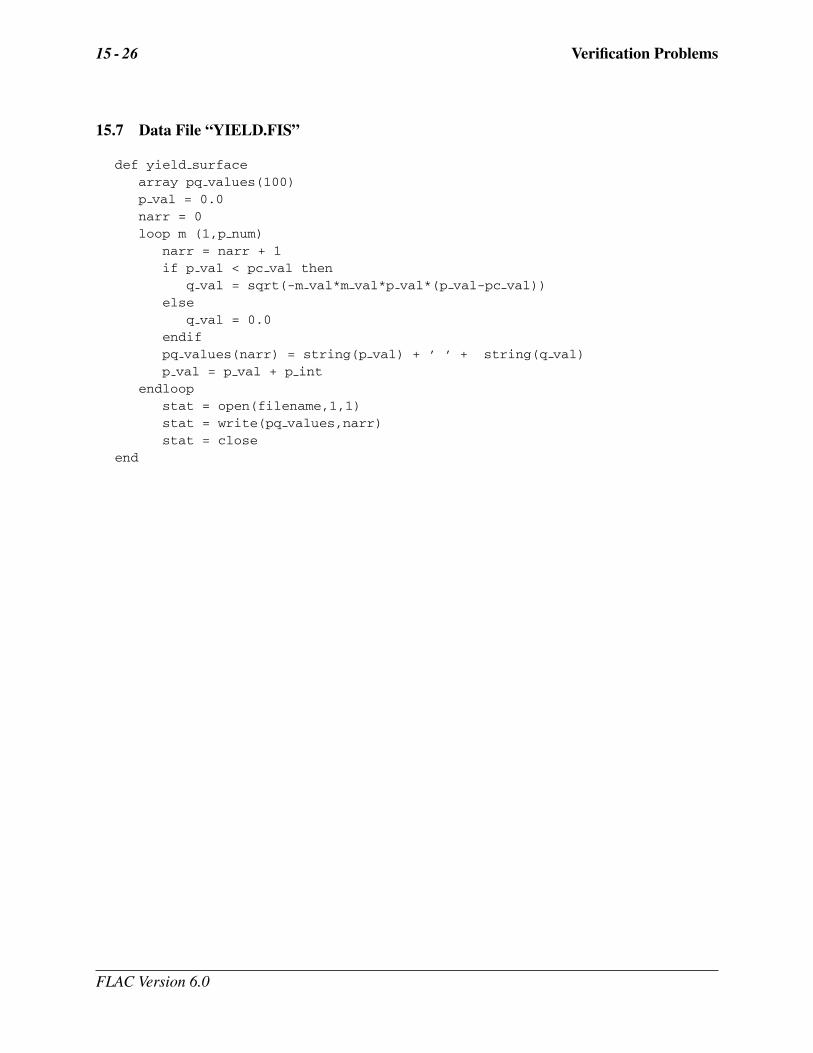
15.7 Data File “YIELD.FIS”

def yield surfacearray pq values(100)p val = 0.0narr = 0loop m (1,p num)

narr = narr + 1if p val < pc val then

q val = sqrt(-m val*m val*p val*(p val-pc val))else

q val = 0.0endifpq values(narr) = string(p val) + ’ ’ + string(q val)p val = p val + p int

endloopstat = open(filename,1,1)stat = write(pq values,narr)stat = close

end

FLAC Version 6.0

verification problems : 15 : drained and undrained ...web.mst.edu/~norbert/ge5471/assignments/assign...

Documents