version 03/12/07 - simon fraser university

Version 03/12/07

John Charles Fields: A Sketch of His Life and

Mathematical Work

by

Marcus Emmanuel Barnes

B.Sc., York University 2005

a Thesis submitted in partial fulfillment

of the requirements for the degree of

Master of Science

in the Department

of

Mathematics

c© Marcus Emmanuel Barnes 2007

SIMON FRASER UNIVERSITY

2007

All rights reserved. This work may not be

reproduced in whole or in part, by photocopy

or other means, without the permission of the author.

APPROVAL

Name: Marcus Emmanuel Barnes

Degree: Master of Science

Title of Thesis: John Charles Fields: A Sketch of His Life and Mathe-

matical Work

Examining Committee: Dr. Jamie Mulholland

Chair

Dr. Tom Archibald

Senior Supervisor

Dr. Glen Van Brummelen

Supervisory Committee

Dr. Jason Bell

Internal Examiner

Date of Defense: November 29, 2007

ii

Abstract

Every four years at the International Congress of Mathematicians the prestigious

Fields medals, the mathematical equivalent of a Nobel prize, are awarded. The fol-

lowing question is often asked: who was Fields and what did he do mathematically?

This question will be addressed by sketching the life and mathematical work of John

Charles Fields (1863 - 1932), the Canadian mathematician who helped establish the

awards and after whom the medals are named.

iii

Dedication

To The Tortoise — keep on plugging along...

iv

Acknowledgments

Many people helped me through the writing of this thesis — to many to list here.

You know who you are and I thank you very much for all the help you have given me.

However, certain individuals do need specific mention. First, I would like to thank my

supervisor, Prof. Tom Archibald. Without his guidance, this document would never

have been completed. He also aided me in several tasks of translating German into

English, including the reviews quoted in Chapter 5 of Fields’ work. Also, I would like

to mention two members of my family who have been my support “on the ground”, so

to speak, here in Vancouver during my studies: my mother, Heather, and my brother,

Steven. I would also like to mention the staff in the department of mathematics at

Simon Fraser University: they were always kind and helpful throughout my studies

there.

I would further like to acknowledge the help of the staff at the University of Toronto

Archives and James Stimpert of the Milton J. Eisenhower Library at Johns Hopkins

University with help finding material related to Fields. The Milton J. Eisenhower

library kindly let me use the portrait of Fields in their collection. Lastly, I would like

to thank my examiners for their comments on a draft version of this document.

v

Contents

Approval . . . . . . . . . . . . . . . . . . . . . . . . . . . . . . . . . . . . . ii

Abstract . . . . . . . . . . . . . . . . . . . . . . . . . . . . . . . . . . . . . iii

Dedication . . . . . . . . . . . . . . . . . . . . . . . . . . . . . . . . . . . . iv

Acknowledgments . . . . . . . . . . . . . . . . . . . . . . . . . . . . . . . . v

Contents . . . . . . . . . . . . . . . . . . . . . . . . . . . . . . . . . . . . . vi

List of Figures . . . . . . . . . . . . . . . . . . . . . . . . . . . . . . . . . . viii

1 Introduction . . . . . . . . . . . . . . . . . . . . . . . . . . . . . . . . 2

I A Biographical Sketch of John Charles Fields 6

2 Fields’ Youth and Education . . . . . . . . . . . . . . . . . . . . . . . 7

2.1 Field’s Youth . . . . . . . . . . . . . . . . . . . . . . . . . . . 7

2.2 Graduate Study at Johns Hopkins University . . . . . . . . . 8

2.3 Post Doctoral Studies in Europe . . . . . . . . . . . . . . . . . 12

3 Professor Fields: 1900-1932 . . . . . . . . . . . . . . . . . . . . . . . 19

II A Sketch of John Charles Fields’ Mathematical Con-

tributions 26

4 Skill in manipulations . . . . . . . . . . . . . . . . . . . . . . . . . . . 29

4.1 Fields’ PhD Thesis . . . . . . . . . . . . . . . . . . . . . . . . 304.1.1 Finite Symbolic Solutions. . . . . . . . . . . . . . . . 324.1.2 Finite Solutions of d3y

dx3 = xmy. . . . . . . . . . . . . . 364.1.3 Solutions by Definite Integrals . . . . . . . . . . . . . 39

4.2 Some of Fields’ Other Early Mathematical Work . . . . . . . . 45

vi

4.2.1 A Proof of the Theorem: The Equation f(z) = 0 Has

a Root Where f(z) is any Holomorphic Function of z 454.2.2 A Proof of the Elliptic-Function Addition-Theorem . 474.2.3 Expressions for Bernoulli’s and Euler’s Numbers . . . 504.2.4 Summary of Fields’ Early Mathematical Work . . . . 52

5 Fields’ Work in Algebraic Function Theory . . . . . . . . . . . . . . . 54

5.1 Elements of Algebraic Function Theory . . . . . . . . . . . . . 56

5.2 Fields’ Theory of Algebraic Functions . . . . . . . . . . . . . . 64

6 Conclusion: The Legacy of J. C. Fields . . . . . . . . . . . . . . . . . 71

Appendix . . . . . . . . . . . . . . . . . . . . . . . . . . . . . . . . . . . . 76

A A Note on Fields’ Berlin Notebooks . . . . . . . . . . . . . . . 76

B The Fields Medal . . . . . . . . . . . . . . . . . . . . . . . . . 76

Bibliography . . . . . . . . . . . . . . . . . . . . . . . . . . . . . . . . . . 78

vii

List of Figures

Fig. 1: John Charles Fields (1863-1932). c© Ferdinand Hamburger Archives

of The Johns Hopkins University . . . . . . . . . . . . . . . . . 1

Fig. 2.1: A drawing in one of Fields’ notebooks showing branch cuts styl-

ized as a bug. UTA (University of Toronto Archives), J. C.

Fields, B1972-0024. . . . . . . . . . . . . . . . . . . . . . . . . 16

Fig. 2.2: A drawing in one of Fields’ notebooks showing branch points

stylized as a map of the Berlin subway stops in the 1890s. UTA

(University of Toronto Archives), J. C. Fields, B1972-0024. . . 17

Fig. 2.3: A page from Fields’ notebook of Hensel’s lectures on algebraic

functions for 1897-98 showing a diagram of a Newton polygon for

an algebraic function. UTA (University of Toronto Archives), J.

C. Fields, B1972-0024. . . . . . . . . . . . . . . . . . . . . . . . 18

Fig. 3.1: J. C. Fields’ gravestone:“John Charles Fields, Born May 14,

1863, Died August 9, 1932.” c© Carl Riehm. Used with per-

mission. . . . . . . . . . . . . . . . . . . . . . . . . . . . . . . 25

Fig. 4.1: Figure from ([Fie86b], 178). . . . . . . . . . . . . . . . . . . . . 46

Fig. 5.1: An depiction of the Riemann Surface for the square root function.

From [AG29, 27]. . . . . . . . . . . . . . . . . . . . . . . . . . . 62

Fig. 6.1: The Fields Medal given to Maxim Kontsevich in 1998 in Berlin.

c©International Mathematical Union. Used with permission . . 77

viii

1

Figure 1: John Charles Fields (1863-1932). c© Ferdinand Hamburger Archives of TheJohns Hopkins University

Chapter 1

Introduction

Many a mathematician has heard of the foremost award in the mathematical sciences,

one often said to be the “Nobel prize” for mathematics, namely, the Fields medal.

Few people, mathematicians included, have any idea of exactly who the mysterious

Fields was. It may come as a surprise to some that this medal was named after a

modest Canadian professor of mathematics at the University of Toronto, John Charles

Fields (1863-1932).

Unfortunately, little is known about Fields, except what appears in the stan-

dard biographical account of his life, an obituary by J. L. Synge [Syn33]. Much of

Fields’ correspondence must be presumed missing or destroyed after it was distributed

upon his death in 1932 (many of his possessions were sent to his brother in Califor-

nia [Fie33]). However, the historian is fortunate on some levels. Fields left many

notebooks of lectures he either attended or copied from others from a postdoctoral

sojourn in Germany in 1890s, spending most of this time in Berlin. There are also

files of the minutes of the Toronto International Congress of Mathematics meeting

committee held in the archives of the International Mathematical Union, which have

allowed scholars like Henry S. Tropp in [Tro76] and Olli Lehto in [Leh98] to detail

the early history of the Fields medals and Fields’ role in the organization of the 1924

2

CHAPTER 1. INTRODUCTION 3

International Congress of Mathematicians, held in Toronto. For a look at modern

mathematics in the light of the Fields medals, see Michael Monastyrsky’s book on the

subject [Mon97].

Other literature on Fields includes an entry on Fields by Tropp in the Dictionary of

Scientific Biography [Tro74]. There is also a small number of general interest accounts

of Fields’ life and his role in the creation of the Fields medals, and these include articles

by C. Riehm [Rie] and by Barnes [Bar03]. Those interested in biographical details

of Fields should consult the first part of this thesis, which is primarily biographical

in nature. The apparent neglect of work on Fields can be attributed in part to the

fact that Fields’ research did not use the prevailing methods of his time and would

ultimately would be subsumed by other more modern approaches. As a result, his

mathematical work has been off the radar of many historians of mathematics.

Regarding Fields’ mathematical contributions, it should be noted that Fields’

postdoctoral studies in Germany would have a decisive influence on his more mature

mathematical work, in particular, Fields’ choice to concentrate on algebraic function

theory, to which he was given an extensive introduction in Germany by some of the

foremost researchers in the area at the time. Fields spent most of his time in Berlin

during his postdoctoral stay in Germany. (The standard reference on mathematics

in Berlin in the nineteenth century is Kurt-R. Biermann’s study [Bie73].) Fields’

ideas are an outgrowth of the lectures contained in his notebooks from Germany.

This was a bit of an about face for Fields, as he had done his initial research work

on differential equations, writing a thesis entitled “Symbolic Finite Solutions and

Solutions by Definite Integrals of the Equation dnydxn

= xmy,” which was published in

the American Journal of Mathematics in 1886 [Fie86c]. Following the completion of

his doctoral work, he continued along similar lines of thought, using the “symbolic

approach in analysis”. For more on this topic, the reader should consult Elaine

Koppelman’s account of the history of the calculus of operations [Kop71], the paper


by Patricia R. Allaire and Robert E. Bradley on symbolical algebra in the context

of the work of D. R. Gregory [AB02], and I. Grattan-Guiness’s chapter on operator

methods [GG94], as well as Boole[Boo44], a general account of this method by one

of its early proponents, George Boole (1815 - 1864). In the 1890s, Fields wrote

on several topics, including a couple of papers in number theory. From 1900 on,

Fields wrote almost exclusively on algebraic function theory. This work of Fields

can be considered as a study of algebraic curves; thus it comprises an episode in the

history of algebraic geometry. Jean Dieudonne in [Die85] has written on algebraic

geometry from its prehistory in ancient Greece to its modern theoretical conception

in the mid-twentieth century, though Fields’ work is not mentioned. Jeremy J. Gray

in [Gra98] and [Gra87] has written on the history of the Riemann-Roch theorem, a

classical nineteenth century result of theoretical importance to algebraic geometry.

Israel Kleiner in [Kle98] has written on the introduction of algebraic ideas, such as

ideals and function fields, into algebraic geometry. Fields’ mathematical contributions

will be discussed chronologically in more detail in part two of this work.

In terms of the context in which Fields functioned as a mathematician during his

lifetime, there are several important works that should be read. For an extensive

background on progress made on linear differential equations in the nineteenth cen-

tury, a topic that would occupy the young Fields, one should consult Jeremy J. Gray’s

volume [Gra99]. Karen Hunger Parshall and David E. Rowe have written a volume

on the emergence of the American mathematical research community [PR94]. The

account includes a discussion of Johns Hopkins University, the school where Fields

chose to do his PhD work, as well as an account of the phenomenon of North Ameri-

can students seeking PhD level training abroad in Germany, something Fields would

do himself in the 1890s. Thomas Archibald and Louis Charbonneau have written the

most complete preliminary survey of the early history of the Canadian mathematical

community before 1945 [AC95]. Fields appears in their account with respect to the


establishment of research level mathematics in Canada. For an history of the mathe-

matics department at the University of Toronto, the school where Fields spent most

of his professional career, one should consult Robinson’s work [Rob79].

We will learn from the sketch of Fields’ life and mathematical work, that although

he was a modest mathematician in both influence and wealth, Fields ultimately left

a very real and important contribution to the modern mathematical landscape, es-

pecially for the mathematical community in Canada, by “recognizing the scientific,

educational, and economic value” [Abo07] of mathematical research. Fields was a

crusader on behalf of this cause, which enabled him (along with the help of others) to

secure the first governmental research support for mathematics in Canada. For this

reason and others, a world renowned mathematical research institute was named in

his honour — The Fields Institute for Research in Mathematical Sciences, located in

Toronto, Ontario, Canada.

Part I

A Biographical Sketch of John

Charles Fields

6

Chapter 2

Fields’ Youth and Education

2.1 Field’s Youth

John Charles Fields was born in Hamilton, Ontario, then Canada West, in 1863, the

son of John Charles Fields and his wife, Harriet Bowes. The Fields family lived at 150

King St. East, his father operating a leather shop at nearby 32 King St. West. Both

of these buildings no longer exist. There is a Ramada Inn where the family house was

located and Jackson Square now occupies the spot where the leather shop once was

[Abo07].

J. L. Synge, a friend and colleague of Fields’, wrote in his obituary that in his

youth, Fields “indulged extensively in sports, baseball, football, hockey, etc.,” and

while in Australia “learned how to throw a boomerang” [Syn33, 156].

Fields attended secondary school at Hamilton Collegiate where he showed an early

talent in mathematics. Following this, in 1880, Fields continued his education by be-

ginning an undergraduate degree at the University of Toronto. In his history of higher

education in Canada Harris paints a picture of what the curriculum was like during

7

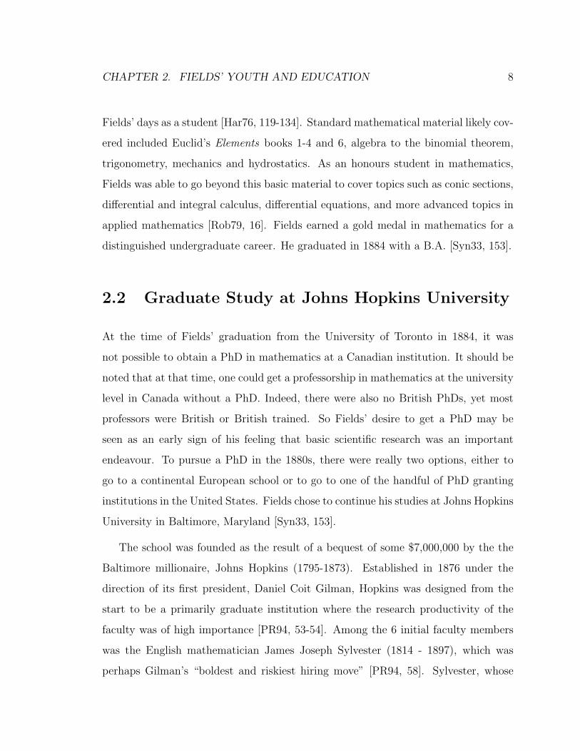
CHAPTER 2. FIELDS’ YOUTH AND EDUCATION 8

Fields’ days as a student [Har76, 119-134]. Standard mathematical material likely cov-

ered included Euclid’s Elements books 1-4 and 6, algebra to the binomial theorem,

trigonometry, mechanics and hydrostatics. As an honours student in mathematics,

Fields was able to go beyond this basic material to cover topics such as conic sections,

differential and integral calculus, differential equations, and more advanced topics in

applied mathematics [Rob79, 16]. Fields earned a gold medal in mathematics for a

distinguished undergraduate career. He graduated in 1884 with a B.A. [Syn33, 153].

2.2 Graduate Study at Johns Hopkins University

At the time of Fields’ graduation from the University of Toronto in 1884, it was

not possible to obtain a PhD in mathematics at a Canadian institution. It should be

noted that at that time, one could get a professorship in mathematics at the university

level in Canada without a PhD. Indeed, there were also no British PhDs, yet most

professors were British or British trained. So Fields’ desire to get a PhD may be

seen as an early sign of his feeling that basic scientific research was an important

endeavour. To pursue a PhD in the 1880s, there were really two options, either to

go to a continental European school or to go to one of the handful of PhD granting

institutions in the United States. Fields chose to continue his studies at Johns Hopkins

University in Baltimore, Maryland [Syn33, 153].

The school was founded as the result of a bequest of some $7,000,000 by the the

Baltimore millionaire, Johns Hopkins (1795-1873). Established in 1876 under the

direction of its first president, Daniel Coit Gilman, Hopkins was designed from the

start to be a primarily graduate institution where the research productivity of the

faculty was of high importance [PR94, 53-54]. Among the 6 initial faculty members

was the English mathematician James Joseph Sylvester (1814 - 1897), which was

perhaps Gilman’s “boldest and riskiest hiring move” [PR94, 58]. Sylvester, whose


mathematical career had been frustrated by his Jewish descent, came out of retirement

to join the faculty at Johns Hopkins in 1877. As a researcher, Sylvester did important

work in invariant theory, number theory, and the theory of partitions. The symbolical

or algebraic approach was an important element of his work. At Hopkins, he was set

the task of establishing the Department of Mathematics as a place where students

could pursue graduate research degrees. He also founded and ran a journal, which

would become known as the American Journal of Mathematics [Par06, 1-8, 225-

277]. Some of Fields’ early publications appeared in this journal. Among Sylvester’s

first batch of graduate students were Fabian Franklin (1853-1939) and Thomas Craig

(1855-1900), both of whom would go on to teach Fields at Hopkins, though Craig

would teach the majority of graduate courses to Fields. Even though Sylvester left in

1883, a year before Fields attended Johns Hopkins, he would influence Fields’ early

mathematical work indirectly, as can be seen by the largely symbolical approaches to

differential equations and differential coefficients in Fields’ work.

Fields arrived at Hopkins in 1884. Fortunately, for many years, lists of classes and

their participants were listed in the Johns Hopkins University Circulars. From this

source we learn that Fields participated in the following courses and seminars:

First half, 1884-85 [Cir84]

Course: Instructor/Organizer:

Analytical and Celestial Mechanics S. Newcomb

Mathematical Seminary W. Story

Theory of Numbers W. Story

Modern Synthetic Geometry W. Story

Mathematical Seminary T. Craig

Calculus of Variations T. Craig

Theory of Functions T. Craig

Problems in Mechanics F. Franklin


Second half, 1884-85 [Cir85b]


Analytic and Celestial Mechanics S. Newcomb

Mathematical Seminary S. Newcomb


Quaternions W. Story

Modern Algebra W. Story


Linear Differential Equations T. Craig


First half, 1885-86 [Cir85a]


Practical and Theoretical Astronomy S. Newcomb


Finite Differences and Interpolation W. Story

Advanced Analytic Geometry – Higher Plane Curves W. Story



Second half, 1885-86 [Cir86b]


Practical and Theoretical Astronomy S. Newcomb


Theory of Probabilities W. Story

Advanced Analytic Geometry W. Story



Elliptic and Abelian Functions T. Craig


First Half, 1886-87 [Cir86a]



Abelian Functions T. Craig

Second half, 1886-87 [Cir87]



Among the textbooks used for the courses Fields took are treatises on differential

equations by Briot, Bouquet, Floquet, and Fuchs; treatises on the theory of functions

by Hermite, Broit and Bouquet, Fuchs, and Tannery; and treatises on elliptic and

Abelian functions by Cayley and by Clebsch and Gordan. The mathematical seminars

were topic based, so that in the second half of the 1884-1885 and 1885-86 years Fields

was registered for two different seminars. As can be seen from the tables of courses,

Fields took many while pursuing his graduate degree. This pattern of participating

in many courses would continue during his study tour in Germany in the 1890s.

Fields received his Ph.D. degree in 1887 with a thesis entitled “Symbolic Finite

Solutions and Solutions by Definite Integrals of the Equation dny/dxn = xmy.” There

is no record of who Fields’ thesis supervisor was, but it was likely Thomas Craig.

There are a couple of reasons to suspect this. First, Craig had research interests

in differential equations, the subject of Fields’ PhD thesis. Second, Craig was the

instructor for most of the courses Fields took while at Hopkins. Other facts that

might be pertinent are that Fields’ first article published in a mathematical journal

was in fact a bibliography on linear differential equations (which he wrote with H. B.

Nixon while at Hopkins [FN85]), and that Fields also later wrote a review of Craig’s

book on linear differential equations [Fie91b]. It is also interesting to note that the

topics of many of the courses Fields took with Craig would later be most closely


related to Fields’ mature research work, namely his work on the theory of algebraic

functions. All this said, the issue of the identity of Fields’ PhD supervisor is still not

fully resolved.

After graduating, Fields became a Fellow at Hopkins (which required a certain

amount of undergraduate teaching duties), a position he held until 1889, at which

point he was appointed Professor of Mathematics at Allegheny College, a small liberal

arts college located in Meadville, Pennsylvania.

He remained in Meadville until 1892, when he resigned his position. The reason

for his resignation was that Fields came into a modest inheritance from his father

and mother, who died when Fields was 11 and 18 years old respectively [Syn33, 153].

He used his inheritance to pursue post-doctoral studies in Europe. With economical

living habits, Fields was able to extend his European studies over 10 years. Fields

was well known to be abstemious, “avoiding tea, coffee, alcohol, and condiments, and

he did not smoke” [Syn33, 156]. The small amount of money he saved from being so

abstemious surely helped him extend his stay somewhat.

With regards to Fields’ mathematical output during the years from 1884 to 1893,

he produced thirteen publications. These papers include a bibliography of linear

differential equation co-authored with fellow Johns Hopkins graduate student H. B.

Nixon in 1885 and a paper based on Fields’ PhD thesis on symbolic finite and definite

integral solutions to the equation dnydxn

= xmy in 1886. Both papers appeared in the

pages of the American Journal of Mathematics.

2.3 Post Doctoral Studies in Europe

It is unclear where Fields spent portions of his 10 year study period in Europe. The

standard obituary by J. L. Synge states that Fields spent 5 years in Paris and 5 years

in Berlin [Syn33, 153]. However, no documentary evidence for his stays in Paris have


come to light.1 It was possible to attend the lectures offered at the College de France

without having to enrol or pay fees [Arc10, 121]. We do have documentary evidence

for Fields’ study period in Germany. Fields enrolled in Gottingen in November 1894,

where he remained until May 1895. There he had the opportunity to attend lectures

by Felix Klein (1849-1925) on number theory, as well as an introductory course on the

theory of functions of a complex variable offered by the Privatdozent Ritter. Fields’

short stay in Gottingen is interesting, as at the time, Gottingen was the destination

of choice for American students pursing studies in mathematics in Germany. For a

discussion of this phenomenon, see the fifth chapter of [PR94]. Fields’ next stop,

Berlin, was much less popular. One possible explanation for Fields’ choice of Berlin

is the fact that L. Fuchs (1833-1902) and Georg Frobenius (1849-1917) were there.

They were both at the forefront of research in linear differential equations, a subject

for which Fields showed an early interest.

We are rather well informed on Fields’ mathematical activities in Berlin, mostly

because a large number of notebooks from this time survive in the Archives at the

University of Toronto. Not all these notebooks were taken from lectures Fields at-

tended. Some of the notebooks tend to be more complete, neat, and do not betray

signs of wandering attention. These books might be transcriptions from the notes of

others. That said, most are arguably first-hand transcriptions.

The notebooks include five courses given by G. Frobenius (1849 - 1917): two on

number theory; one on analytic geometry; and two on algebraic equations. There are

are notebooks of nine courses given by L. Fuchs (1833 - 1902), including the theory of

hyperelliptic and Abelian functions, and topics on differential equations, many related

to Fuchs’ own work. There are notebooks of six courses given by Kurt Hensel (1861-

1941), including algebraic functions of one and two variables, a course on Abelian

integrals, and a course on number theory. Hensel’s lectures related closely to Fields’

1Tom Archibald – personal communication.


later research work. There are notebooks of fifteen courses given by H. A. Schwarz

(1843-1921), on such topics as elliptic functions, variational calculus, the theory of

functions of a complex variable, synthetic projective geometry, number theory, and

integral calculus. Fields also has notes of two courses from G. Hettner (1854-1914) on

definite integrals and Fourier series, two courses from J. Knoblauch (1855-1915) on

curves and surfaces, and a course from E. Steinitz (1871-1928) on Cantor’s theory of

transfinite cardinals.2 In addition to these notebooks we have almost an entire series

of lectures by M. Planck, an early edition of what would later be his famous course

on theoretical physics; two courses on inorganic chemistry; and one on the history of

philosophy.

In the notebooks, Fields took his notes in a mixture of English and German. Some

notebooks are rather sketchy, while others, such as those on Schwarz’s course on the

calculus of variations, are rather complete. And as always, there are the usual signs

of a student’s mind wandering (for example, see Figures 2.1 and 2.2).

Though the notebooks provide a useful historical resource, Fields makes regret-

tably few remarks as to his reactions to the material and to his professors. However,

Fields’ later research work shows the signs of the influence of K. Weierstrass (1815

- 1897) and K. Hensel. Fields’ approach to algebraic function theory used several

function-theoretic techniques for representing functions along the lines of the work of

Weierstrass, but at the same time, Fields’ aim was a theory that was arithmetical in

nature, the approach favoured by Hensel.

It is interesting to note that Fields’ education, both at Johns Hopkins University

and during his European study tour, was rich in material that would later become

useful for him in his research on algebraic function theory, as a quick glance at the

titles of the courses he participated in attests.

2The birth and death years for some the instructors of the courses contained in Fields’ notebookshave been gleaned from [Sch90].


In terms of Fields’ mathematical output during his post-doctoral studies in Europe,

Fields did not publish any papers during the years 1894 to 1900, though he seems

to have continued to do research, presenting a talk at the meeting of the American

Mathematical Society held in Toronto in 1897 on the reduction of the general Abelian

integral. He would publish a paper based on this talk in 1901, which would mark the

beginning of his mature mathematical research work [Fie01]. It is not really surprising

that Fields failed to publish during the years 1894-1900, given the number of courses

he apparently attended, as can be ascertained from large number of notebooks full of

lecture notes he accumulated during this time.


Figure 2.1: A drawing in one of Fields’ notebooks showing branch cuts stylized as abug. UTA (University of Toronto Archives), J. C. Fields, B1972-0024.


Figure 2.2: A drawing in one of Fields’ notebooks showing branch points stylized as amap of the Berlin subway stops in the 1890s. UTA (University of Toronto Archives),J. C. Fields, B1972-0024.


Figure 2.3: A page from Fields’ notebook of Hensel’s lectures on algebraic functionsfor 1897-98 showing a diagram of a Newton polygon for an algebraic function. UTA(University of Toronto Archives), J. C. Fields, B1972-0024.

Chapter 3

Professor Fields: 1900-1932

Fields took up a position as special lecturer at the University of Toronto in 1902. At

that time the mathematics department had roughly five members including Fields

[Rob79, 14]. By 1905 he had gained a regular position as Associate Professor and

would later become Professor in 1914 and Research Professor in 1923 [Syn33, 153],

153. Among the honours that Fields received was election to the Royal Society of

Canada in 1909 and to the Royal Society of London in 1913 [Enr85, 139].

Fields apparently predominantly taught higher level courses. In Robinson’s history

of the University of Toronto Mathematics Department [Rob79, 18-19] he quotes at

length from Norman Robertson, a Toronto lawyer who was born in Orangeville in

1893 and graduated from the University of Toronto in 1914. It is worth quoting parts

of this here to give an idea of Fields’ teaching style. Robertson reports that in his day

in the mathematics and physics program at the university, Fields “did not present any

lectures to the earlier years, but lectured to us on differential equations and perhaps

quaternions in third and fourth years.” Furthermore, Fields “on entering the Lecture

Room... armed himself with a large, wet sponge in the left hand, and a piece of chalk

in the right hand, and without preliminary, he started at the left panel of the Board,

with his back to the class, addressing his remarks to the work he was inscribing on the

19

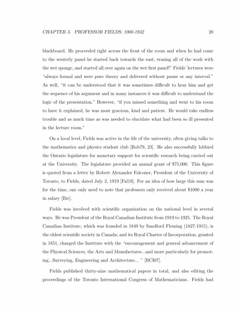
CHAPTER 3. PROFESSOR FIELDS: 1900-1932 20

blackboard. He proceeded right across the front of the room and when he had come

to the westerly panel he started back towards the east, erasing all of the work with

the wet sponge, and started all over again on the wet first panel!” Fields’ lectures were

“always formal and were pure theory and delivered without pause or any interval.”

As well, “it can be understood that it was sometimes difficult to hear him and get

the sequence of his argument and in many instances it was difficult to understand the

logic of the presentation.” However, “if you missed something and went to his room

to have it explained, he was most gracious, kind and patient. He would take endless

trouble and as much time as was needed to elucidate what had been so ill presented

in the lecture room.”

On a local level, Fields was active in the life of the university, often giving talks to

the mathematics and physics student club [Rob79, 23]. He also successfully lobbied

the Ontario legislature for monetary support for scientific research being carried out

at the University. The legislature provided an annual grant of $75,000. This figure

is quoted from a letter by Robert Alexander Falconer, President of the University of

Toronto, to Fields, dated July 2, 1919 [Fal19]. For an idea of how large this sum was

for the time, one only need to note that professors only received about $1000 a year

in salary [Rie].

Fields was involved with scientific organization on the national level in several

ways. He was President of the Royal Canadian Institute from 1919 to 1925. The Royal

Canadian Institute, which was founded in 1849 by Sandford Fleming (1827-1915), is

the oldest scientific society in Canada; and its Royal Charter of Incorporation, granted

in 1851, charged the Institute with the “encouragement and general advancement of

the Physical Sciences, the Arts and Manufactures...and more particularly for promot-

ing...Surveying, Engineering and Architecture... ” [RCI07].

Fields published thirty-nine mathematical papers in total, and also editing the

proceedings of the Toronto International Congress of Mathematicians. Fields had


several other publications that were printed versions of addresses he gave to the Royal

Canadian Institute. These include his presidential address on “Universities, Research

and Brain Waste” which was delivered on November 8th, 1919 at a meeting of the

Royal Canadian Institute. In the talk he laments the state of university level research

in Canada and the waste of the potential of Canadian scientists and engineers. He

discusses what can be done to help rectify the situation by using examples from

European schools.

On the international level, Fields was Vice-President of both the British Asso-

ciation for the Advancement of Science in 1924 and the American Association for

the Advancement of Science, Section A in 1924. The goal of both organizations is

roughly to advance public understanding, accessibility and accountability of the sci-

ences and engineering. More importantly than these presidencies, Fields brought the

International Mathematical Congress of 1924 to Toronto.

The account that follows of the International Mathematical Union and the Toronto

International Congress of Mathematicians is based on Olli Lehto’s volume [Leh98, 23-

37] on the history of the Union. In 1919 in Brussels in the wake of World War One,

the International Research Council was established. The aim was to be a kind of cen-

tral control of the international scientific community with responsibility for overseeing

international meetings as part of its mandate. The first president of the Council was

the mathematician Emile Picard (1856 - 1941). It was at the constitutive meeting

in Brussels that the International Mathematical Union was established, the initial

executive being C. de la Vallee Poussin (1866 - 1962) and W. H. Young (1863 - 1942).

Included among the statutes of the IMU was that the Union was to provide the or-

ganization for the ICMs. The statutes of both the International Research Council

and the International Mathematical Union excluded the central powers of Germany,

Austria-Hungary, Bulgaria, and Turkey due to the animosities resulting from the first


great war. As a result, no scientists from these countries could participate in inter-

national scientific meetings held under the auspices of the Council, a situation that

persisted until June 29, 1926, when an Extraordinary General Assembly of the Coun-

cil was held in Brussels and the exclusionary statutes on membership were deleted

([Leh98], 40).

The first ICM after World War I was held in Strasbourg, France, in 1920. The

Congress was soaked in political controversy because of the exclusionary clauses of

the Union. Many mathematicians were loud in their opposition to the exclusionary

clauses of the IMU, such as G. H. Hardy (1877 - 1947), stating that “All scientific

relationships should go back precisely to where they were before [the war].... ” (Quoted

from [Leh98, 30]). Gosta Mittag-Leffler was also among the more prominent and

influential mathematicians opposed to the exclusion of the “central powers”. This

political controversy carried over to the International Congress in Toronto.

The American delegates to the Strasbourg General Assembly of the Union offered

to host the 1924 Congress without first consulting the American Mathematical Society.

The Society was not fully supportive of holding the Congress in the United States

because of the political controversy. By 1922 it was felt that the political climate

would have made financial backing unattainable in the United States because of the

restrictions on participation in the Congress as a result of the exclusionary clauses of

the Union. The American Mathematical Society withdrew its support for organizing

the Congress.

Fields apparently jumped at the opportunity to organize the Congress, which

was to be held in Toronto in 1924 despite the political controversy [Leh98, 33-37]. A

colleague of Fields’, Professor J. L. Synge of the University of Toronto, wrote: “I do not

think that he himself approved strongly of the prohibitory clauses in the regulations

of the Union; indeed, I feel confident that he would have welcomed the opportunity


of organizing a truly international congress in Canada” [Syn33, 154].1 However, his

desire to have the meeting in Canada apparently outweighed his reservations. Fields

took it upon himself to help promote the conference. He travelled across the Atlantic

several times before the congress in order to arrange details personally and to help

gain the participation of important figures. Incidentally, Fields travelled overseas

many times during his adult life. There is an amusing anecdote about an incident

during one such trip, which appeared in print in The Star on August 10, 1932, in

a short article entitled “Death Claims Noted Savant at University”. The anecdote

is as follows: “Dr. Fields was a bachelor, and an amusing story is told of his ‘love

affairs’ abroad. On one occasion, while abroad, he arranged to meet Professor Love

at a certain hotel. When Dr. Fields arrived there, the girl clerk presented him with

a telegram reading: Sorry, I cannot meet you, Love. The doctor treasured this

evidence of his ‘love affairs.’”2

The Toronto congress was quite successful with 444 people registered, which is

over double the first post-war meeting in Strasbourg. For comparison, 574 mathe-

maticians had been in attendance at the last Congress before World War One, held

in Cambridge, England in 1912, an event Fields attended [Leh98, 15]. Of the 444

registrants of the Toronto Congress, approximately 300 were from North America.

Part of the Congress was an excursion across Canada, from Toronto to Victoria on

Vancouver Island. Fields put much work into guaranteeing that the Toronto Congress

would be a success.

After the 1924 Congress, Fields’ health began to deteriorate. With the help of

colleagues, Fields was able to complete the proceedings of the Toronto Congress, which

1Fields wrote in 1930 that he “visited a number of European mathematicians during the Summerwith a view to learning more of the international situation as it affects mathematics” and thathe “happens to be persona grata to the Germans as well as to the French” and that it occurredto him “that it might be possible to do something towards smoothing things out and bringing arapprochement” [Fie30, 4].

2Augustus Love (1863 - 1940), a British mathematician, held the Sedleian chair of natural philos-ophy at Oxford starting in 1899. He did important research on the mathematical theory of elasticityand geodynamics.


appeared in two large volumes in 1928, though as Fields shared in the prefatory note in

the first volume of the proceedings, it “was an unexpected and none too welcome task

which fell to the lot of the undersigned [i.e., Fields] when circumstances determined

that he should edit the Proceedings” [Fie28]. The work fell mostly on Fields’ shoulders

due to the fact his colleague, Professor J. L. Synge, General Secretary of the Congress,

was leaving Toronto for a job as chair at Trinity College, Dublin and it was felt that

the duty of editing the proceedings should be undertaken by someone in Toronto who

could see the proceedings through the press [Fie28].

On February 24, 1931, in the minutes of a meeting of the organizing committee,

it was first reported that, after meeting the expenses of holding the Congress and

publishing the Proceedings, there was a positive balance of $2,700. The committee

then continued its report by stating its intention to use most of this money to estab-

lish two medals to be awarded at, and in connection with, successive International

Mathematical Congresses [Tro76, 170].

At the next recorded meeting of the committee (with Fields still chairman) on

January 12, 1932, Fields reported that the major mathematical societies of the U.S.,

France, Germany, Switzerland, and Italy had indicated support for the introduction

of an international medal in mathematics. A memorandum entitled “International

Medals for Outstanding Discoveries in Mathematics” attached to the minutes of the

meeting and signed by Fields, outlined the idea of the medals. In this memorandum,

it was stated that the medals “should be of a character as purely international and im-

personal as possible.” And further that “there should not be attached to them in any

way the name of any country, institution or person [Tro76, 174].” Obviously, Fields’

wish that the medals should not be named after a person was ignored. The memo-

randum further set out the nature of the awards, that one should “make the awards

along certain lines not alone because of the outstanding character of the achievement

but also with a view to encourage further development along these lines [Tro76, 174].”


Figure 3.1: J. C. Fields’ gravestone:“John Charles Fields, Born May 14, 1863, DiedAugust 9, 1932.” c© Carl Riehm. Used with permission.

It was Fields’ successful fund-raising for the Congress that was to make the initial

steps towards the establishment of the Fields medals. There was a further source

of initial funds: Fields organized not only the ICM, but also a second conference, a

meeting of the British Association for the Advancement of Science, held in September

1924 in Toronto. In the end, part of the surplus money went to the Royal Canadian

Institute to fund research (Toronto Mail,, May 4, 1925). Eventually $2500 of the

surplus would go towards the medals [Tro76, 170].

Fields died in Toronto on August 9, 1932, apparently from a stroke. He was buried

in Hamilton Cemetery, which overlooks the western end of Lake Ontario (at “Cootes

Paradise”, where McMaster University also sits). His simple gravestone is about

22 inches by 16 inches and is set flat on the ground. It reads “John Charles Fields,

born May 14, 1863, died August 9, 1932.” A passer-by, reading this very modest stone,

would have no idea of Fields’ influence on the mathematical and scientific community.

Upon his death, Fields left an estate of $45071, a large part of which went towards the

medals.3 He left his brother with a small annuity, and his maid Julia Agnes Sinclair,

widow, a small pension as long as she remained unmarried. He left the money to be

used towards the awards in the hands of Professor Synge and the prime minister of

Canada.

3Toronto Star, Sept. 30, 1932.

Part II

A Sketch of John Charles Fields’

Mathematical Contributions

26

27

As previously noted, Fields published thirty-nine mathematics-related publications

[Syn33, 159- 160]. Fields’ published mathematical work can be divided into two

periods: from 1885 to 1893 and from 1901 to 1928. The year 1885 marks the year of

his first publication, a bibliography on linear differential equations that was published

in the American Journal of Mathematics. The year 1928 marks a publication in

the proceedings of the International Congress of Mathematicians in Bologna, Italy.

After 1928, Fields’ health was poor and his mathematical output more or less ended.

The years 1894 to 1900 mark Fields’ post-doctoral studies in Europe. That Fields

failed to publish anything during this time can be accounted for by the many courses

he apparently took, as his large collection of lecture notes attests. That said, he

apparently did some research during his European study tour, presenting some of this

work at the American Mathematical Society meeting in Toronto held in 1897. The

work presented at the meeting would later mark the beginning of the publication of

his more mature mathematical work in 1901 [Fie01, 49].

The period 1885-1893 will concern us in Chapter Four. A generalization of Ric-

cati’s equation was the topic of Fields’ PhD thesis, which we will examine in section

4.1. In addition to this work, Fields published proofs of some well known theorems

such as the elliptic function addition-theorem and the fundamental theorem of algebra.

These two papers plus an another one on Euler and Bernoulli numbers will be dis-

cussed in section 4.2. Fields published other work during the years 1885 to 1893, such

as his papers entitled “A Simple Statement of Proof of Reciprocal-Theorem” [Fie91c],

“Transformation of a System of Independent Variables” [Fie92], and “The numbers

of sums of quadratic residues and of quadratic non-residues respectively taken n at a

time and congruent to any given integer to an odd prime modulus p” [Fie93], but we

will not have occasion to discuss them here.

After Fields’ post-doctoral studies in Europe, he concentrated almost entirely on

the theory of algebraic functions and the related theory of Abelian integrals. The

28

period 1901-1928, as noted earlier, marks the publication of Fields’ more mature

mathematical work. The theory of algebraic functions and Fields’ conception of the

theory will the the focus of Chapter Five.

In the final chapter, we will try to answer the question of whether Fields’ mathe-

matical work had any sort of influence or lasting legacy. It will be argued that despite

the fact that Fields’ approach ultimately did not gain wide use in further research

within the mathematical community, his work did play another and important role for

mathematics, and especially for the developing Canadian mathematical community.4

4S. Beatty has written that Fields “by his insistence on the value of research as well as by theimportance of his published papers, has, perhaps, done most of all Canadians to advance the causeof mathematics in Canada” [Bea39, 109].

Chapter 4

Skill in manipulations

In this chapter we will look at some of Fields’ early research work. At this point in

his career, Fields was still trying to establish himself as a research mathematician and

he still had not narrowed in on what would become his main research program.

Fields published his first paper in 1885, written with H. B. Nixon, a fellow graduate

student in the mathematics department while Fields was at John Hopkins University,

in the American Journal of Mathematics, which had just been established in 1878 as

the first research level journal in North America devoted solely to mathematics. The

paper was an extensive bibliography of work on linear differential equations [FN85].

Fields would go on to publish several other papers that would appear in this journal.

As Fields’ student S. Beatty would observe in his summary of the mathematical

contribution of his former teacher, Fields’ early papers “offer simplifications of existing

treatments, while others give extensions, secured chiefly by skill in manipulation”

[Syn33, 156].

29

CHAPTER 4. SKILL IN MANIPULATIONS 30

4.1 Fields’ PhD Thesis

Fields’ PhD thesis, entitled “Symbolic Finite Solutions and Solutions by Definite

Integrals of the Equation dny/dxn = xmy”, was among those of his papers published in

the American Journal of Mathematics. Finite solutions are in closed form, unlike those

expressed in series or as integrals. The meaning of the term “symbolic” solution is not

so easy to grasp. We will try to untangle the meaning in section 4.1.1, primarily by

example. Solutions by definite integrals, also known as solution by “quadratures,” are

solutions by integrals where boundary conditions on the integrals have been specified.

For a survey of the history of ordinary differential equations, one may consult Kline

([Kli90a], 468-501, 709-738), Archibald [Arc03], and Gilain [Gil94].

The equation dnydxn

= xmy, which is the focus of Fields’ thesis, is similar to certain

Riccati equations. Jacopo Riccati (1676-1754), an Italian nobleman and mathemati-

cian, studied certain second order differential equations. The differential equation

dy

dx= Ay2 +Bxn,

A and B constant, became known as Riccati’s equation [BD77, 7][Gil94, 441-442]. In

generalized form it is usually written as

dy

dx= a0(x) + a1(x)y + a2(x)y2.

L. Euler (1707 - 1783) showed that by a suitable change of function, the generalized

Riccati equation and the second-order homogeneous linear differential equation are

equivalent [Gil94, 442]. This amounted to showing that the general Riccati equation

dw

dx= q0(x) + q1(x)w + q2(x)w2,

leads to the second-order linear homogeneous equation

q2(x)y′′ − [q′2(x) + q1(x)q2(x)] y′ + q22(x)q0y = 0,


via the transformation w = −y′/yq2 [BD77, 112]. If q2(x) = 1 and q1(x) = 0, then

this last equation reduces tod2y

dx2+ q0(x)y = 0. (4.1)

This clarifies the connection to Fields’ equation

dny

dxn= xmy

and (4.1). Rather than taking a second-order equation, we take an nth order equation,

and we set q0(x) = −xm for some m.

As Fields points out at the beginning of his thesis, the finite solutions obtained

are analogous to the symbolic solutions of Riccati’s equation. As J. W. L. Glaisher

notes in his 1881 survey article on Riccati’s equation, many symbolic solutions to

Riccati’s equation had been given, by (for instance) R. L. Ellis, Boole, Lebesgue,

Hargrave, Williamson, Donkin, and Gaskin [Gla81, 762]. Glaisher discusses some of

these symbolic solutions in the sixth section of his survey. It should be pointed out

that Fields’ symbolic solutions to the equation under investigation in his thesis are

rather more complicated than those of the Riccati equation presented in [Gla81], in

large measure because Fields considers an nth order equation instead of simply a

second-order equation.

In the last half of the nineteenth century, linear differential equations was a topic

that received much attention from some of the world’s leading research mathemati-

cians, though the main breakthroughs were generated by considering the differential

equations in terms of functions of complex variables, rather than simply of real vari-

ables as in Fields’ work [Gra99]. Fields would go on to hear lectures by some of these

researchers in Berlin during his European study tour in the 1890s, including lectures

by L. Fuchs, Frobenius, and Schwarz. He also attended a lecture course by Klein

while spending a year in Gottingen and seems to have at least communicated with H.

Poincare, another researcher who made fundamental progress on the theory [Gra99].

In a letter to D.C. Gilman, President of Johns Hopkins University, Baltimore, Fields


writes that “Poincare has also in his hands at present a paper on the ‘change of any

system of independent variables’, which he has kindly promised to present before the

Societe Mathematique de France” [Fie]. The paper of Fields’ that he was referring to

was [Fie92].

4.1.1 Finite Symbolic Solutions.

The basic idea of the symbolic method is to treat the operations of analysis, such

as differentiation, as if they were operators or symbols. These operators can then

be manipulated in ways analogous to the way variables are treated in basic algebra.

Fields uses operator methods extensively in his thesis, as well as in some of his early

research papers, such as [Fie89].

The operator idea goes back at least as far as the work of Gottfried Wilhelm

Leibniz (1646 - 1716) on the differential d operating on a variable x to produce the

infinitesimal dx. In fact, Koppelman in [Kop71, 158-159] traces the the history of

the “calculus of operations” back to a letter dated 1695 by Leibniz, addressed to

Johann Bernoulli, that discusses the analogy between raising a sum to a power and

the differential of a product. The development of the basic results in the calculus of

operators is mainly of French origin. Joseph Louis Lagrange (1736 - 1813) stated many

of the initial results. Lagrange’s results were later proven by P. S. Laplace in 1776

[Kop71, 159-160]. Lagrange’s work helped spark other work in this area by French

mathematicians, including that by L. F. A. Arbogast (1759 - 1803), B. Brisson (1777 -

1828), and Augustin Louis Cauchy (1789 - 1857). In 1807, Brisson pioneered the idea

of thinking of a differential equation as a differential operator on a function from which

one could use the algebra of operators to produce solutions. Later, Cauchy founded

operator based procedures similar to Brisson’s [GG94, 545-546][Kop71, 158-175].


Operator based methods were particularly attractive to English and Irish mathe-

maticians in the nineteenth century. Building on the work in the 1830s by R. Murphy

and D. F. Gregory (1813 - 1844), George Boole’s paper “On a General Method in

Analysis,” which appeared in the Philosophical Transactions of the Royal Society in

1844, examined in depth the basic ideas of the differential operator method [Boo44].

He noted that these operators obey three properties: commutativity, distributivity,

and the index law (that is, that DnDm = Dm+n, m and n positive integers), though

care had to sometimes be taken with respect to commutativity.

Many mathematicians used differential operator methods to solve differential equa-

tions. For example, Pierre Simon Laplace (1749 - 1827) used such methods in his

research into the shape of the Earth. By the end of the nineteenth century, ba-

sic methods were included in textbooks, such as R. D. Carmichael’s A Treatise on

the Calculus of Operations (1855) and Boole’s A Treatise on Differential Equations

(1859) and A Treatise on the Calculus of Finite Differences ([GG94], 548). It should

be noted that Fields was likely familiar with Boole’s text. In Robinson’s history of

the University of Toronto mathematics department appears a list of material taught

during Alfred Baker’s days there, and among the texts listed is Boole’s text on dif-

ferential equations [Rob79, 16].1 One might venture a guess that Fields came across

some of the material in these books during his early mathematical education, since

using textbooks from England was the norm in Canada.

The principal hope with using differential operator methods to solve differential

equations was to be able to express solutions in finite form rather than as infinite

series. The overall success of the differential operator approach was somewhat limited

however, since many important differential and difference equations were not easily

solved using these methods [GG94, 548].

1Baker joined the staff at the University of Toronto in October 1875 as a Mathematical Tutor. Soit is likely he taught the undergraduate Fields. Baker went on to become a professor of mathematicsat the university and a senior colleague of Fields’ [Rob79, 16].


To help illustrate the differential operator method as applied to differential equa-

tions, we will look at the equation

d2y

dx2+ 3

dy

dx+ 2y = 0, (4.2)

which is discussed briefly in [AB02, 414-415] in the context of a more general discussion

of D. F. Gregory’s “symbolical algebra”, which is essentially the same set of methods

as we have been referring to as the symbolical method or the operational calculus.

The basis of the symbolical method in analysis is the technique of the separation

of symbols. This technique consisted of distinguishing between two essential types of

symbols, corresponding to the modern notion of functions and linear operators. The

later were to be separated from the former in order to help derive and prove theorems

in analysis [AB02, 403]. When we apply the technique of separation of symbols to

(4.2), we get the auxiliary equation

(D2 + 3D + 2)y = 0,

where were have denoted the differential operator ddx

by D. Note that in the last

equation we have separated the differential operator from the function y. Now this

expression can be factored to give us

(D + 1)(D + 2)y = 0,

from which we recognize the particular solutions y = e−x and y = e−2x to be the

solutions to (D + 1)y = 0, (D + 2)y = 0. The general solution is then the linear

combination of the two particular solutions [AB02, 414-415]. Of course this is but a

simple example and the operational calculus is in general much more difficult, but this

example highlights the basic technique, which when applied skilfully, can generate

results like those discussed in Fields’ doctoral thesis. For a more thorough look

at symbolical methods in analysis, one should consult Boole’s writings [Boo44] and

[Boo59], as well as the papers by Koppelman [Kop71] and Allaire and Bradley [AB02]

which give a historical perspective on the method.


Having now seen an example of a basic application of symbolical methods to the

solution of differential equations, we will set forth two basic results that Fields uses

during the course of his dissertation, to which we will have chance to refer later on.

Result 4.1 The general solution to an nth order homogeneous differential equation

with constant coefficients,

y(n) + an−1y(n−1) + · · ·+ a1y

′ + a0y = 0

whose characteristic roots λ1, . . . , λn are all distinct, is

y = c1eλ1x + c2e

λ2x + · · ·+ cneλnx

for some constants c1, . . . , cn.

The proof of this result and related results for when the characteristic roots are not

distinct can be found in any standard text on differential equations, for example

([Bro93], chapter 9).

Result 4.2 Given a function f in terms of x, we have

eddxf(x) =

(1 + h

d

dx+

1

1 · 2h2 d

2

dx2+ · · ·

)f(x) = f(x+ h).

As Boole points out [Boo59, 389] no direct meaning can be given to the expression

eddxf(x), but if one were to treat the exponent d

dxas a quantity, the result follows

from Taylor’s theorem. We can interpret the symbolical terms in the parenthesis as

performing an operation on the function f . It should be noted that each of these

operational symbols can actually be carried out, even though doing so may be very

labour intensive. The symbol eddx is often dealt with very much like the symbol eAt,

where A is a square matrix, as treated in modern theories of linear operators such as

that presented in [DS58], namely,

eAt = In +1

1!At+

1

2!A2t2 + · · · =

∞∑n=0

1

n!Antn.


4.1.2 Finite Solutions of d3ydx3 = xmy.

Fields’ thesis work is good example of what “skill in manipulations” can achieve

[Syn33, 156]. However, this makes reading his thesis research rather long and tiresome,

as one must go through every single detail of those quite lengthy manipulations. Fields

breaks his discussion of symbolic finite solutions of dnydxn

= xmy into two parts, one for

the case n = 3 in order to give a more concrete impression of his technique, the second

for the equation of the nth order. Luckily for Fields, his technique for n = 3 generalizes

quite nicely to the nth order case. For sake of the exposition, we will abbreviate his

argument for n = 3. Throughout his thesis, Fields considers the symbols such as dd∆

and(dd∆

)−1which obey the commutative and distributive laws.

The first step in finding a solution when n = 3 is to suppose that

d3y

dx3= xmy (4.3)

is satisfied by the series y =∑anx

nα where α = m + 3. Using standard series

methods, this gives

y =∞∑n=0

α−3nxnα

n!(1 + ν1) · · · (n+ ν1)(1 + ν2) · · · (n+ ν2), (4.4)

where ν1 = −1α

, and ν2 = −2α

.

At this point, Fields introduces the symbol ∆ =(ddz

)−1so that

∆nzm =zm+n

(1 +m) · · · (n+m).

By setting z = α−3xα in (4.4), Fields is able to find that

y =∑ z−ν∆nzν2

n!(1 + ν1) · · · (n+ ν1)(4.5)

= z−ν2∆−ν1

∑(dd∆

)−nn!

·∆ν1 = z−ν2∆−ν1e(dd∆)

−1

∆ν1 · zν2 , (4.6)

where “the functional symbol ∆−ν1e(dd∆)

−1

∆ν1 is supposed to operate upon zν2” [Fie86c,

368]. Fields does not explain the nature of the dd∆

operator. One possible way to make


sense of it is to note that since ∆ =(ddz

)−1, we have that

d

d∆=

d

d(ddz

)−1 =d

d(dzd

) =d

dz.

What exactly does one do in order to operate upon zν2 with ∆−ν1e(dd∆)

−1

∆ν1? One

first applies ∆ν1 to zν2 , to the result Φ(z) of which, one then applies e(dd∆)

−1

, which

means roughly, “expand using Taylor’s theorem” to get(1 +

(d

d∆

)−1

+1

2

(d

d∆

)−2

+ · · ·

)Φ(z).

This expansion follows from (Result 4.2). One then applies ∆−ν1 , which can also be

written as(ddz

)ν1 , to the preceeding, which roughly means “differentiate the expression

term by term ν1 times.”

This settled, Fields then shows that if the right hand side of (4.6) is “known and

finite” [Fie86c, 368] for given values ν1, ν2 (arbitrary), then the expression also holds

for all values of ν1, ν2 differing from those given values by integers. Thus if the new

values are ν1 − i, ν2 − k, then one can simply apply the operation

zi−ν1

(d

dz

)izν1−ν2+k

(d

dz

)kzν2

to the known function containing the values ν1 and ν2 to get new values of the function

[Ham07].

At this point, Fields narrows in on actual solutions to d3ydx3 = xmy. He is able to

do this by noting that in the previous equation, if m = 0, then y is known, so either

ν1 = −13, ν2 = −2

3or ν1 = −2

3, ν2 = −1

3. In the first case, we must have that

−1

3− i =

1

−α= − 1

m+ 3, −2

3− k = − 2

α,

from which one can conclude that m = −9i3i+1

. Similarly, in the second case, we have

that m = −3(3i+1)3i+2

. In both cases, the differential equation is solvable in finite terms

for any whole number i [Ham07].


We may summarize Fields’ results from the first portion of his thesis as follows.

The general solutions of (4.3) are

Case 1: m = −9i3i+1

y = x

(x1− 3

3i+1d

dx

)ix1+ 3i

3i+1

(x1− 3

3i+1d

dx

)2i

x−2

3i+1 (4.7)

×(C1e

−(3i+1)λ1x1

3i+1+ C2e

−(3i+1)λ2x1

3i+1+ C3e

−(3i+1)λ3x1

3i+1

); (4.8)

Case 2: m = −3(3i+1)3i+2

y = x

(x1− 3

3i+2d

dx

)ix1− 3i

3i+2

(x1− 3

3i+2d

dx

)2i+1

x−1

3i+2 (4.9)

×(C1e

−(3i+2)λ1x1

3i+2+ C2e

−(3i+2)λ2x1

3i+2+ C3e

−(3i+2)λ3x1

3i+2.

)(4.10)

where in the above, the Cis are arbitrary constants and the λis are here the cube

roots of unity.

Having dealt with dnydxn

= xmy for the case n = 3, Fields moves on in the next

section of his thesis to deal with nth order case. Luckily, the techniques used by

Fields in the case n = 3 generalize well, but things get messier. But again, with the

assumption that the solution to (4.3) is known for m = 0, Fields is able to show that

(4.3) is solvable in finite form for all values of

m =−n(ni+ k − 1)

ni+ k,

where k is a whole number less than and relatively prime to n, and i is an arbitrary

integer [Ham07].

In the next section of his dissertation, using the methods suggested by the ideas

developed in the first part of his thesis, Fields solves a couple of simpler differential

equations, the details of which need not occupy us here.


4.1.3 Solutions by Definite Integrals

A solution to a differential equation is said to be a solution by definite integrals if

the solution (a function) is written as a definite integral (possibly a multiple definite

integral). This form of solution also sometimes referred to as solving a differential

equation by quadratures, especially in older literature. Solving differential equations

by definite integrals arguably has been used since the foundational work by G. Leibniz

(1646 - 1716) and I. Newton (1643 - 1727) on the calculus, specifically with their

work on the fundamental theorem of calculus.2 The methods of Leibniz in particular

were expanded upon by Johann and Jakob Bernoulli, and then shortly thereafter

by L. Euler (1707 - 1783). These three individuals studied physical phenomena via

differential equations and as a result contributed many of the elementary results of

differential equations, including solutions by definite integrals. For more on this see

[Jah03], [Arc03], and [Gil94].

Fields’ results in this section are a generalization of results obtained by E. Kum-

mer (1810 - 1893) and Spitzer for the solution of dnydxn

= xmy by definite integrals.

Furthermore, by using some of the methods from the first part of his thesis, Fields is

able to give particular solutions in definite integrals for given values of m.

In order to get a better grip on what Fields accomplishes in this section, it will

be worthwhile to look at the work of Kummer’s that Fields cites, namely [Kum39].

Kummer’s paper builds on the work of R. Lobatto in [Lob37] who posed dnydxn

= xmy

as an object of further research in mathematical analysis [Kum39]. Kummer only

considers the case where m is a positive integer. Spitzer finds the general solution in

definite integral form when m has absolute value greater than 2n.

Kummer’s results, stated right at the beginning of his paper are the following. If

2Much has been written on Leibniz and Newton’s work on the calculus. For more on this, oneshould consult [Gui03], [Gui94], and Newton’s collected mathematical papers with notes by D. T.Whiteside [New81].


z = Ψ(x) is a general solution of

dn+1z

dxn+1= xm−1z, (4.11)

then the general solution of the equation

dny

dxn= xmy (4.12)

can be expressed by the definite integral

y =

∫ ∞0

um−1e−um+n

m+n Ψ(xu) du, (4.13)

where the n+1 constants of integration satisfy a certain relation and where the limits

of integration have been chosen to “make things work out.”

In order to demonstrate his result, Kummer begins thus. First differentiate (4.12)

to getdn+1y

dxn+1= xm

dy

dx+mxm−1y. (4.14)

Substituting into this last equation the expressions for y, dydx

and dn+1ydxn+1 , and observing

that equation (4.11) gives us

dn+1Ψ(xu)

dxn+1= xm−1um+nΨ(xu),

we get

xm−1

∫ ∞0

u2m+n−1e−um+n

m+n Ψ(xu) du (4.15)

= xm∫ ∞

0

e−um+n

m+n Ψ′(xu) du+mxm−1

∫ ∞0

um−1e−um+n

m+n Ψ(xu) du. (4.16)

As Kummer points out, one can verify the preceding equation by first differenti-

ating ume−um+n

m+n Ψ(xu) in terms of u to get

d(ume−

um+n

m+n Ψ(xu))

= mum−1e−um+n

m+n Ψ(xu) du

−u2m+n−1e−um+n

m+n Ψ(xu) du+mume−um+n

m+n Ψ′(xu) du.


By now multiplying this equation by xm−1 and integrating from 0 to ∞, we get

(4.15)-(4.16).

Thus the expression given in (4.13) for y is the general solution of (4.14), and as

a consequence also expresses the general solution of (4.12), if the n + 1 constants of

integration satisfy a certain relation.

At this point, Kummer works out the condition on the constants of integration,

case by case, successively using his result above and the solution of the equation

dnzdxn

= z. Designating the solution of dnzdxn

= z by Ψ(n, x), we get the well known result

that

Ψ(n, x) = Cex + C1exe

2πin + C2e

xe4πin + · · ·+ Cn−1e

xe2(n−1)πi

n .

Thus the main result of Kummer paper states that the solution to

dny

dxn= xy

is given by

y =

∫ ∞0

e−un+1

n+1 Ψ(n+ 1, xu) du.

From the fact that dnydxn

= 0 when x = 0, we find the relation among the n+1 constants

of integration, namely

C + e−2πin+1C1 + e−

4πin+1C2 + · · ·+ e−

2nπin+1 Cn = 0.

For the case m = 2, the solution of

dny

dxn= x2y

is

y =

∫ ∞0

∫ ∞0

ve−un+2+vn+2

n+2 Ψ(n+ 2, xuv) du dv,

and since dnydxn

= 0 and dn+1

dxn+1 = 0 when x = 0, one gets two equations giving relations

among the constants of integration, namely

C + e−2πin+2C1 + e−

4πin+2C2 + · · ·+ e−

2(n+1)πin+2 Cn+1 = 0

C + e−4πin+2C1 + e−

8πin+2C2 + · · ·+ e−

4(n+1)πin+2 Cn+1 = 0.


In the same manner, one can find the relations among the constants of integration for

m = 3, 4, . . ..

Spitzer’s result is based on Kummer’s method above, but is slightly modified in

order to show that if Ψ(x) is the general solution of

xm+1 dn+1z

dxn+1= εz,

then the general solution of xm dnydxn

= −εy may be expressed by∫ ∞0

um−1e−um−nm−n Ψ

(xu

)du,

again with a certain relation holding among the (n+1) constants of integration. Thus

as Fields points out, Spitzer has found the definite integral form of the solution of

dnydxn

= xmy for all negative integer values of m with absolute value greater than 2n

[Fie86c, 383].

Fields expresses the results of Kummer and Spitzer in combination as follows. If

Ψ(x) is the general solution of dn+1

dxn+1 = bxm−1z, then the general solution of dn

dxn= axmy

may be expressed as

y =

∫ ∞0

um−1e−baum+n

m+n Ψ(xu) du, (4.17)

where there is a certain relation holding among the n + 1 constants of integration

where m+ n and m are of the same sign, and ba

is positive or negative depending on

whether this sign is a plus or minus [Fie86c, 384].

Fields points out that this result may be easily verified by differentiating dn

dxn−

axmy = 0 and then substituting in the expression for dn+1

dxn+1 , the expression for y′ and

y from (4.17).

Summarizing the known results, Kummer’s solution of dnydxn

= xmy covers the case

where m and m + n are positive, and Spitzer’s the case where m and m + n are

negative. However, both Kummer and Spitzer assume that that n must be a positive

integer. But as Fields remarks, in the verification of (4.17), there is no requirement


that n must be positive. So n may be negative as long as m and m + n still satisfy

Kummer’s or Spitzer’s conditions. What this means then, is that from the solution

of d−n+1zdx−n+1 = xm−1z, one may derive the solution of d−ny

dx−n= xmy. By substituting

xm−1z = v into the two previous equations, we get x−m+1v = dn−1vdxn−1 and x−mu = dnu

dxn.

Thus, we see that from the solution of dn−1vdxn−1 = x−m+1v we may derive the solution of

dnudxn

= x−mu, where in stating this, Fields assumes that in carrying out the operation

d−nydx−n

, the constants of integration will always be set equal to zero, so that the solutions

of y = dn

dxn(xmy) are the solutions of d−ny

dx−n= xmy.

In the following, Fields makes use the (then well known) result that the solution

of dnydxn

= x−2ny is y = xn−1∑Cre

−µrx , and the result that the solution of d−n

dx−n= x2nz

is z = x−2ny = x−n−1∑Cre

−µrx , where the µs are the nth roots of unity and the Cs

are arbitrary constants. Starting with the equation

d−nz

dx−n= x2nz,

and using (4.17), we may express the solution of d−n−1ydx−n−1 = x2n+1y as

y = x−n−1

∫ ∞0

un−1e−un

n

∑Cre

−µrxu du.

By successively applying (4.17) we may obtain the solution of d−n−i

dx−n−i= x2n+iy,

y = x−n−1

∫ ∞0

∫ ∞0

· · ·∫ ∞

0

i∏κ=1

un+κ−2k e−

1n

Piκ=1 u

nk

∑Cre

−µr(xu1···ui)−1

du1du2 · · · dui.

By substituting n for (n + i) into the previous equation we get that the solution

of d−nydx−n

= x2n−iy may be expressed as

y = x−n+i−1

∫ ∞0

· · ·∫ ∞

0

i∏κ=1

un−i+κ−2κ e−

1n−i

Piκ=1 u

n−iκ∑

Cre−µr(xu1···ui)−1

du1du2 · · · dui,

(4.18)

where by∏i

κ=1 un−i+κ−2κ Fields means the product un−i−1

1 un−i2 · · ·un−2i and where i is

always a positive integer less than n, and the µis are the (n− i)th roots of unity.


For dn

dxn= x−2n+iu we have u = x2n−iy, and therefore we have for the equation

dny

dxn= x−2n+iy (4.19)

the solution

y = xn−1

∫ ∞0

· · ·∫ ∞

0

∏κ=1

iun−i+κ−2κ e−

1n−i

Piκ=1 u

n−ik

∑Cre

−µr(xu1···ui)−1

du1 · · · dui.

(4.20)

Hence, by deriving (4.20), Fields has derived a definite integral solution of the

equation dnydxn

= xmy for all negative integer values of m between n and 2n, thus

extending the results of Kummer and Spitzer. Fields notes that the solution he gives

is not the most general one because the constant of integration when operating by

d−1

dx−1 was always set equal to zero, but that the solution still contains −(m+n) = n− i

arbitrary constants.

Having established the more general solution, Fields now takes some time to find

particular solutions of dnydxn

= xmy for any value of m. In particular, he establishes

that the equationdny

dxn= x−my (4.21)

has a solution given by

y = xn−1

∫ ∞0

· · ·∫ ∞

0

u2u23 · · ·un−2

n−1e1

n−m(um−n1 +···+um−nn−1 +(xu1···un−1)n−m) du1 · · · dun−1

(4.22)

where m is any positive quantity greater than n.

At this point, Fields remarks that we can find similar solutions for other values of

m by starting with d−1ydx−1 = xmy, where m − 1 is any negative quantity, and then by

successively using formula (4.17) with ab

= −1.

Using some of his results from the first part of his thesis on finite symbolic solutions

of the nth order equation dnydxn

= xmy, Fields is now able to establish that if we proceed

along similar lines by starting from some equation whose solution is known, either


finitely or as a definite integral, then we can derive solutions for dnydxn

= xmy for any

real value of m expressed as integrals in various forms [Ham07].

4.2 Some of Fields’ Other Early Mathematical Work

Before moving on to discuss Fields’ more mature work on the theory of algebraic

functions, we will pause here briefly to look at a small selection of Fields’ other early

publications. In many of his early publications, Fields’ proves known results. There

are a couple of reasons why he may have done this. As any young academic knows,

being able to say that you are a published scholar helps. So Fields may have written

these papers to help establish his reputation as a mathematician. It is also conceivable

that, as a graduate student and then fellow of the Johns Hopkins University, he

was helping to fill the pages of the young American Journal of Mathematics, which

only began publication in 1878 under the auspices of the university and the editorial

leadership of Johns Hopkins based mathematicians.3

4.2.1 A Proof of the Theorem: The Equation f(z) = 0 Has a

Root Where f(z) is any Holomorphic Function of z

This paper, which appeared in the pages of the American Journal of Mathematics

in February 1886 [Fie86b], was written while Fields was still at Johns Hopkins Uni-

versity. The theorem, when restricted to polynomials, is basically a statement of the

fundamental theorem of algebra, which says that every polynomial equation p(z) = 0

has a complex number solution. With this theorem, one is able to factor polynomials

into linear factors over the complex numbers, or equivalently, as a product of linear

and irreducible quadratic factors over the real numbers. This result was used without

3For more details on the early history of the American Journal of Mathematics, see [PR94, 88-94].


Figure 4.1: Figure from ([Fie86b], 178).

proof for a long time. The first mathematicians who tried to prove the theorem rig-

orously were Jean Le Rond d’Alembert (1717-1783) and C. F. Gauss (1777 - 1855),

though their initial attempts are far from satisfactory from a modern perspective

([Sti89], 196). Fields’ proof is but one of many different proofs of the fundamental

theorem of algebra. For others, see [FR97].

Fields begins by letting z be a point in one complex plane A with origin o and

f(z) = ζ a point in another complex plane B with origin ω. Recall that a holomorphic

function is synonymous with an analytic function, a function which can be represented

by a convergent Taylor series expansion at every point. If f(z) = ζ cannot become

equal to zero for any value of z, then Fields observes that there is some minimum

distance from the origin ω within which ζ cannot fall. As he points out, we can

suppose this, since f(z) becomes infinite as z becomes infinite, and thus the required

minimum must occur for a finite value of z, and therefore “can be reached” [Fie86b,

178]. Fields now tries to come up with a contradiction.

We will use the modern concept of neighbourhood to simply the exposition slightly.

Fields does not use this terminology in his paper, but what he does write amounts to

basically the same thing.

As indicated in Figure 4.1, about z draw a δz - neighbourhood (where δz denotes


an increment of z). The corresponding δζ-neighbourhood of ζ (see Figure 4.1) is given

by δζ = fr(z)r!

(δz)r, where f r(z) is the first successive derivative of f(z) which does not

vanish for the value of z. The closed curve describing the δζ-neighbourhood about ζ

comes between the point ζ and the origin ω. But this means that the point ζ is not at

the minimum distance to the origin as first supposed. This is a contradiction. Hence

the function f(z) = ζ can become zero and hence the equation f(z) = 0 has a root.

Fields finishes off the paper by giving a slight variation on the final statements of the

proof.

This paper must have been somewhat of a disappointment for Fields, as there

is an addendum at the end of the paper stating that just as the note was to go to

press, Fields discovered that practically the same proof had been given by Houel in

his Cours de Calcul Infinitesimal. Fields had been scooped.

4.2.2 A Proof of the Elliptic-Function Addition-Theorem

Elliptic functions can trace their origin to the study of elliptic integrals, that is,

integrals of the form ∫R[x,√p(x)

]dx,

where R is a rational function and p is a polynomial of degree 3 or 4. The word

“elliptic” refers to a certain class of these integrals that can be interpreted as the

arc-length of an ellipse [Coo94, 529]. The idea of inverting elliptic integrals to obtain

elliptic functions is due to C. F. Gauss, N. H. Abel (1802 - 1829), and C. Jacobi (1804

- 1851), though Abel was the first to publish. Abel’s “Recherches sur les fonctions

elliptiques” appeared in Crelle’s Journal in the fall of 1827. Abel covered much of the

same ground as Gauss had in his unpublished work. Gauss noticed this. On March

30 1829, Gauss wrote to W. Bessel (1784 - 1846) that

It appears that for the time being I won’t be able to get back to the work


on transcendental functions that I have been conducting for many years

(since 1798), since I must first finish up many other things. Herr Abel, I

notice, has now preceded me and has relieved me of approximately one-

third of these things, the more so as he has carried out all the computations

elegantly and concisely. He has chosen the exact same route that I took in

1798; for that reason the large coincidence in our results is not surprising.

To my amazement this extends even to the form and partly to the choice

of notation, so that many of his formulas seem to be exact copies of my

own. To avoid any misunderstanding I note, however, that I do not recall

ever having discussed these things with anyone (quoted in [Kol96, 138]).

Even though Abel covered some of the same ground as Gauss, Abel developed the

theory to a greater extent than Gauss and in a more thorough manner. Abel’s paper

also contains the first published theory of the inverse functions of elliptic integrals

[Kol96, 154].

Around the same time that the first part of Abel’s Researches was published, a note

“Extraits de deux lettres a Schumacher” appeared in the Astronomische Nachrichten

(Number 123) in 1827 by the German C. Jacobi. He detailed without proof a new

result on the transformation of elliptic integrals. In March 1828, Abel read Jacobi’s

proofs of the results in “Demonstratio theorematis ad theoriam functionum ellipti-

carum spectantis” in an issue of Astronomische Nachrichten (Number 127) in 1827.

This was a shock to Abel. There was not much he could do other than quickly publish

his own ideas on the transformation of elliptic integrals. He published his theory, for

which Jacobi’s results are special cases, in “Solution d’un probleme general concer-

nant la transformation des fonctions elliptiques” (Astronomische Nachrichten, which

appeared in two parts, one in volume six in 1828 and one in volume seven in 1829

[Kol96, 156-157]. The priority dispute between Jacobi and Abel would not last long

as Abel succumbed to tuberculosis and died in 1829. Jacobi continued to work on


elliptic functions for most of his career.

Jacobi’s 1829 text Fundamenta nova functionum ellipticarum has garnered Jacobi

the title of co-founder of the theory of elliptic functions. A novel aspect of the theory

of elliptic functions presented in the Fundamenta nova was the initiation of the theory

of theta functions. Jacobi was to use theta functions to give representations of the

three “basic” elliptic functions, later known as sn u, cn u, and dn u, as quotients of

theta functions [Kol96, 158-159].

Just like Gauss and Abel, Jacobi started with the elliptic integral of the “first

kind,” but in what is now know as Legendre normal form,

u = F (φ, k) =

∫ φ

0

dt√1− k2 sin2 t

,

where k is a parameter with 0 < k2 < 1 and φ = F−1(u, k). Jacobi called the

parameter k the modulus and the variable φ the amplitude, which he denoted by

am u. Substituting x = sinφ gives

u =

∫ x

0

dx√(1− x2)(1− k2x2)

.

So for the inverse of the elliptic integral of the first kind, we have x = sin am u, which

is read “sine-amplitude of u”. In a similar way, Jacobi defined the following essential

functions

cos am u =√

1− sin2 am u, 4am u =√

1− k2 sin2 am u,

the cosine-amplitude and the delta-amplitude. In 1838, Christoph Gudermann (1798-

1852), who would mentor K. Weierstrass, gave the now common notation — sn u,

cn u, and dn u — for the three “Jacobi elliptic functions,” in his paper “Theorie der

Modular-Functionen und der Modular-Integrale” which appeared in the J. fur Math.,

volume eight, in 1838. Fields uses Gudermann’s standard notation in his paper on

the addition theorem for elliptic functions.


Recall that the elliptic function addition theorem states that:

sn(u+ v) =snucnvdnv + snvcnudnu

1− k2sn2usn2v.

Fields gives a proof of this result in a paper which appeared in the American Journal

of Mathematics in July 1886 ([Fie86a]). He does this by integrating the differential

equationdφ

∆φ+dΨ

∆Ψ= 0,

where ∆φ =√

1− k2 sin2 φ, etc., using the integrating factor

∆φ∆Ψ− k2 sinφ cosφ sin Ψ cos Ψ

1− k2 sin2 φ sin2 Ψ.

From this he finds that

tanφ∆Ψ + tan Ψ∆φ

1− tanφ tan Ψ∆φ∆Ψ= tanµ,

and observes that since µ = φ when Ψ = 0, µ is the amplitude of (u + v), where u

and v are elliptic functions whose amplitudes are φ, Ψ respectively. From this he is

able to establish quickly that

sn(u+ v) = sinµ =tanµ√

1 + tan2 µ=

sinφ cos Ψ∆Ψ + cosφ sin Ψ∆φ

1− k2 sin2 φ sin2 Ψ,

and, using some standard identities, he proves the theorem. Fields finishes the paper

by commenting that the addition formulas for cn(u+ v) and dn(u+ v) can be just as

readily obtained.

4.2.3 Expressions for Bernoulli’s and Euler’s Numbers

In this paper, which appeared in the American Journal of Mathematics in January,

1891, Fields derives related expressions for the Bernoulli and Euler numbers [Fie91a].

Jakob Bernoulli (1654-1705) in his book Ars Conjectandi (1713), a work on the

subject of probability, introduced what are now called the Bernoulli numbers. In the


course of finding a formula for the sums of the positive integral powers of the integers,

Bernoulli gave the formula

n∑k=1

kc =1

1 + cnc+1 +

1

2nc +

c

2B2n

c−1 +c(c− 1)(c− 2)

2 · 3 · 4B4n

c−3+

c(c− 1)(c− 2)(c− 3)(c− 4)

2 · 3 · 4 · 5 · 6B6n

c−5 + · · · ,

where the series terminates at the last positive power of n. The formula was given

without proof. The numbers

B2 =1

6, B4 = − 1

30, B6 =

1

42, B8 = − 1

30, B10 =

5

66, . . . ,

are the Bernoulli numbers [Kli90a, 451].

The Euler numbers E2m appear in the power series expansion of the secant func-

tion:

sec z =∞∑m=0

(−1)mE2m

(2m)!z2m,

where this power series expansion converges for |z| < π2, and E0 = 1, E2 = −1, E4 = 5,

E6 = −61, etc. Euler numbers, often referred to as secant numbers, were supposedly

first given their name by the influential English mathematician J. J. Sylvester [Ely82,

337].

Both Bernoulli and Euler numbers appear in the sums of several interesting infinite

series that where studied by both Bernoulli and Euler. For example, the Bernoulli

numbers appear in the following sums:

1 +1

22+

1

32+ · · · = B2

2 · 2!(2π)2 =

π2

6,

1 +1

24+

1

34+ · · · = − B4

2 · 4!(2π)4 =

π4

90

and the Euler numbers appear in the following related formulas:4

1− 1

3+

1

5− · · · = E0

2

π

2=π

4,

4For more on the relationship between these two sets of formulas, see [Mar77, 64-66].


1− 1

33+

1

53− · · · = − E2

2 · 2!

(π2

)3

=π3

32.

Fields, referring to a result found in Bertrand’s Calcul Differentiel [Ber64, 141]

(which is also derived in an 1889 paper by Fields in the American Journal of Mathe-

matics), establishes related expressions for Bernoulli and Euler numbers. The result

he refers to is (d

dx

)nφ(u) =

n∑r=1

n∑ρ=r

(−1)ρ−ruρ−rφp(u)

r!(ρ− r)!

(d

dx

)nur.

By setting u = x−ix we get

secx+ tanx =2

u+ i+ i =

∑ Enxn

n!,

where when n is even we get Euler’s number En, and when n is odd, we get Bernoulli’s

number Bn+12

= (n+1)En2n+1(2n+1−1)

.

By substituting θ(u) = 1u+i

in the formula from the start and by a series of ma-

nipulations, Fields is able to find that when n is odd

En = 2

(i

2

)n+12

n+1∑s=2

s−1∑r=1

is+r(n+ 1

s

)rn.

Hence the corresponding expression for Bernoulli’s number is

Bn+12

=2(n+ 1)

2n+1(2n+1 − 1)

(i

2

)n+12

n+1∑s=2

s−1∑r=1

is+r(n+ 1

s

)rn.

Fields finishes off the paper by observing that since En is real, the imaginary terms

in the summations in the last expression for En must cancel. He gives an expression

for En using only real numbers, leaving to readers the exercise of figuring out the

corresponding expression for Bn.

4.2.4 Summary of Fields’ Early Mathematical Work

In the first part of Fields’ mathematical career there is no obvious unifying theme to

his work. He had some papers on number theory such as [Fie91c] and [Fie93], papers


that use the symbolic method in analysis such as [Fie89] and [Fie92], as well as the

papers discussed in sections 4.2.1 – 4.2.3 which provided new proofs to known results.

Though Fields must have felt that research and publication was important, it seems

that he did not finish his studies at Hopkins with a clear idea of where he was headed

mathematically. This was to change after his time in Europe in the mid-1890s, after

which almost all of his research efforts focussed on the theory of algebraic functions.

It is this aspect of Fields’ mathematical career which will occupy us in next chapter.

Chapter 5

Fields’ Work in Algebraic Function

Theory

The theory of algebraic functions grew out of attempts to generalize the theory of

elliptic integrals. Recall from section 4.2.2 that elliptic integrals are integrals of the

form ∫R[x,√p(x)

]dx,

where R is a rational function and p is a polynomial of degree 3 or 4. N. H. Abel was

the first to make significant progress on studying these types of integrals by studying

their inverses. In fact, Abel was able to generalize vastly the theory to integrals I

where the function defining the relation between x and y is any polynomial whatsoever.

These integrals are now called Abelian integrals in his honour. The generalization of

the theory of elliptic integrals turned out to be such a rich area for research that work

done on this and related matters can be seen as one of the major themes of nineteenth

century mathematics, dominating the attention of some of the most highly regarded

mathematicians of the time (e.g., K. Weierstrass).

According to Bliss [Bli24, 96] there are three main approaches to the theory of

54

CHAPTER 5. FIELDS’ WORK IN ALGEBRAIC FUNCTION THEORY 55

algebraic functions: the transcendental, the geometric, and the arithmetic. Bliss’s

perspective on the state of the theory at the turn of the twentieth century is interest-

ing, since, as far as he is concerned, each approach aims at the same thing, but each

with its positive and negative features. In fact, in his book on algebraic functions

[Bli33], Bliss gives each perspective almost equal consideration.

In the transcendental theory, due in large part to the work of Abel and B. Riemann,

Abelian integrals play the key role. The geometrical theory is strongly connected

with the study of higher plane curves, and was developed in the work of Clebsch

and Gordan, and later by mathematicians such as F. Severi (1879 - 1961). In the

arithmetical theories, a slightly misleading name for the approach, the emphasis is

on the construction and theory of rational functions and only secondarily on the

construction of the Abelian integrals for which these functions are the integrands

[Bli24, 96].

The arithmetical approach was first presented by L. Kronecker (1823 - 1891) to

the Berlin Academy in 1862, but was not published until 1881. Other theories using

the arithmetical approach are those of R. Dedekind (1831 - 1916) and H. Weber

(1842 - 1913), K. Weierstrass (1815 - 1897) (developed in his famous lectures but not

appearing until the publication of his collected works), as well as later by Hensel and

Landsberg (who developed and simplified the methods of Dedekind and Weber), and

the theory of our protagonist, J. C. Fields, which was published in book form in 1906

[Fie06][Bli24, 96].

Those who favoured the arithmetical approach often criticized the transcendental

and geometrical theories on the grounds that these two theories required the applica-

tion of an initial birational transformation to a curve described by F (x, y) = 0 in order

to simplify the singular points. The singular points of such curves can be unwieldy

and very complicated in nature [Bli24, 96]. The arithmetical theories were developed

in part to side-step these difficulties, by allowing calculations, often with formal power


series, to provide all the necessary information about the nature of singular points,

though G. Landsberg (1865 - 1912) noted that the power series methods needed to be

rendered algebraic. Modern theories of algebraic functions, which were first worked

out in the 1920s and 1930 by mathematicians such as O. Zariski (1899 - 1986), are

approached mainly using the tools of abstract algebra. The modern methods essen-

tially overshadowed the nineteenth century approaches because of the ability of these

theories to generalize to higher dimensions, unlike arithmetical theories such as that

of Fields.

In this chapter we will try to give an indication of the scope of Fields’ work

in algebraic function theory, or what we might now call algebraic geometry. First

we will briefly discuss the elements of the theory as understood at the beginning

of the twentieth century when Fields undertook the majority of his more mature

mathematical researches and then we will briefly discuss Fields’ approach to the theory

and try to give an indication of how Fields’ work relates to other approaches used at

the time.

5.1 Elements of Algebraic Function Theory

We will use G. A. Bliss’ [Bli33] extensively in this section, as it gives an introduction

to both the arithmetic theory and the transcendental theory of algebraic functions.

More will be said about the differences between the various approaches to studying

algebraic functions at the turn of the twentieth century in the next section.

In what follows, let f(x, y) be a polynomial in y of the form

f(x, y) = f0(x)yn + f1(x)yn−1 + · · ·+ fn(x)

where each coefficient fi(x) is itself a polynomial in x with complex coefficients.


Definition 5.1 (Algebraic Function) An algebraic function is a function y(x) de-

fined for values x in the complex x-plane by an equation of the form f(x, y) = 0 [Bli33,

24].

An algebraic function y(x) is in general multi-valued, meaning that for each value

x in the complex x-plane for which the function is defined, there is more than one value

y in the complex y-plane that corresponds to x. This is contrary to what is observed in

elementary analytic geometry, where the points of a curve in the real xy-plane are in

one-to-one correspondence with pairs of real values (x, y) satisfying the given algebraic

equation f(x, y) = 0 (with real coefficients) that defines the curve. The notion of a

Riemann surface, the type of surface on which an algebraic function “lives”, discussed

below, was developed in order to restore a one-to-one correspondence between points

of the domain and points satisfying f(x, y) = 0 ([Bli33], 75).

Definition 5.2 (Ordinary and Singular Points) A point x = a in the complex

x-plane where f0(a) 6= 0 and the discriminant of f at x = a does not vanish is called

an ordinary point. A point x = a at which one or both of f0(a) and the discriminant

of f at x = a vanish, is called a singular point [Bli33, 25].

The point x = ∞ is ordinary or singular according to whether 0 is an ordinary or

singular point of f(x′, y) = 0, where x′ = 1x. The point at infinity is in general treated

as a point in the complex plane. In what follows, when we speak of the complex plane,

we mean the extended complex plane – the complex plane with the point at infinity

adjoined.

Rational functions are functions of the form P (x, y)/Q(x, y), where P and Q are

polynomials in the complex variables x and y. These form one of the most impor-

tant classes of functions in algebraic function theory. Rational functions have no

singularities in the complex plane other than poles.


Definition 5.3 (Poles) Given an analytic function g(z), suppose g(z0) fails to be

analytic at a point z = z0. If we can find a positive integer n such that limz→z0(z −

z0)ng(z) = A 6= 0, then the point z = z0 is called a pole of order n. If n = 1, z0 is

called a simple pole [Spi64, 67].

For example, the rational function

g(z) =(z − 3)2

(z − 1)3(z − 7),

has a pole of order 3 at z = 1 and a simple pole at z = 7.

It can be shown that when the discriminant of f(x, y) is non-zero for all but a

finite number of values x = a, the values of the algebraic function y(x) are distinct

and exactly n in number [Bli33, 25]. For example, given an algebraic function y(x)

defined by the relation y2 = x, often called the square root function, we see that for

every non-zero finite value of x = a correspond two distinct values of y, respectively

y = +√a and y = −

√a. At x = 0, the discriminant is equal to zero and the two

values of y are not distinct. The two functions y = +√x and y = −

√x are called

the branches of the multi-valued function y(x). More generally, we may consider a

multi-valued function as a collection of single valued functions, each member of which

is a branch of the function.

In the theory of algebraic functions, it is often useful to represent functions in

terms of series expansions. In fact, this is the basis for the arithmetical approaches

to the theory, including Fields’ own. The following is a basic theorem about series

representations of algebraic functions.

Theorem 5.4 In the neighbourhood of an ordinary point x = a the n values of an

algebraic function y(x) are defined by n convergent series

y = bi + ci1(x− a) + ci2(x− a)2 + · · · ,

where the numbers bi are the n distinct roots of f(a, y) and i = 1, . . . , n [Bli33, 25].


It can be shown that similar expansions exist for values of y(x) near a singular

point, but that such series may have terms with negative and/or fractional powers

of x − a [Bli33, 29]. I. Newton (1643 - 1727) showed in De methodis serierum et

fluxionum (1671) that any algebraic function y(x) can be expressed as a fractional

power series in x and gave a method for generating these series expansions using what

are now known as Newton polygons [Sti89, 125-126]. The fractional powers were not

well understood until the variables were taken to be complex and it was not until

the work of V. Puiseux (1820 - 1883) in 1850 [Pui50] that this was more rigorously

clarified [Sti89, 125-126]. One of the more important results proved by Puiseux is the

following:

Theorem 5.5 (Puiseux’s Theorem) In a neighbourhood of a point (x0, y0) of the

domain of an algebraic plane curve f(x, y) = 0, y(x) can be expressed by a finite

number of fractional power series developments

y − y0 = a1(x− x0)q1q0 + a2(x− x0)

q2q0 + · · · ,

which converge in some interval about x0 and all the qi have no common factors. The

points given by each development are called a branch of the algebraic curve [Kli90a,

552-553].

For this reason, fractional power series expansions of algebraic functions are now often

referred to as Puiseux expansions [Sti89, 125-126].

The reason for the failure of ordinary power series to represent algebraic functions

at points that are not ordinary, is that at these points such functions display branching

behaviour. This is a result of the multi-valuedness of such functions. Fractional power

series are able to capture this behaviour.

Using the simple example of the square root function, we can see this behaviour.

Writing our complex numbers in polar form, we have for x = riθ, y =√rei

θ2 . Consider


a point a = r1eiθ1 so that y =

√r1e

iθ12 . By making a full circuit around the origin,

that is by adding 2π to the angle θ1, we arrive at what should be the same point, but

instead we find that y =√r1e

iθ1+2π

2 = −√r1eiθ12 . If we however make another circuit

around the origin, that is add 4π to θ1, we get y =√r1e

iθ1+4π

2 =√r1e

iθ12 [Spi64, 37].

Definition 5.6 (Branch Point, Algebraic Branch Point) A branch point of an

analytic function is a point x = reiθ in the complex plane whose complex argument θ

can be mapped from a single point in the domain to multiple points in the range. An

algebraic branch point is a branch point whose neighbourhood of values wrap around

the range a finite number of times p as their complex arguments varies from 0 to a

multiple of 2π and is said to have order p [Weia], [Weib].

Referring back to Puiseux’s Theorem (5.5), supposing q1/q0 is the smallest exponent

(written in lowest terms) in the fractional series representation of our algebraic func-

tion defined by f(x, y) = 0 about a branch point x = x0, then we can simply read off

the order of the branch point as q0, the denominator of this smallest exponent. This

is in fact the definition used by Paul Appell and Edouard Goursat in their book on

algebraic functions [AG29].

In our example of the square root function, we see that the origin is an algebraic

branch point of order 2. A circuit around any other finite point does not lead to

different values. So we see that the origin is the only finite branch point of the square

root function. So for the square root function, the only finite point about which the

function cannot be represented by a ordinary power series is the algebraic branch

point x = 0. In order to represent the square root function as a power series at

the branch point, one needs to admit fractional exponents in the terms of the series

expansion.

Since the fractional series expansion of the square root function is so simple, it is

worthwhile to look at the series expansion of a more complicated algebraic function


about some of its branch points. Let us consider y2 − x(x − 1)(x − 2) = 0. This

relation defines an algebraic function y(x) with two branches, y1 =√x3 − 3x2 + 2x

and y2 = −√x3 − 3x2 + 2x, which we have labelled with subscripts 1 and 2 for ease

of reference. There are three branch points for each branch. The following are three

such expansions. If we expand y1 and y2 about x = 0 we get1

y1 =√

2x12 − 3

4

√2x

32 − 1

32

√2x

52 − 3

128

√2x

72 − 37

2048

√2x

92 − 117

8192

√2x

112 − · · · ,

and

y2 = −√

2x12 +

3

4

√2x

32 +

1

32

√2x

52 +

3

128

√2x

72 +

37

2048

√2x

92 +

117

8192

√2x

112 + · · · .

If we expand y1 about x = 1, we get

y1 = i(x− 1)12 − 1

2i(x− 1)

52 − 1

8i(x− 1)

92 − 1

16i(x− 1)

132 − 5

128i(x− 1)

172 + · · · .

Having briefly discussed branch points and their orders, it is now useful to define

another piece of important terminology. A branch cut is a portion of a line or curve

(with ends possibly open, half-open or closed) that is introduced into the complex

plane to distinguish between branches of a multi-valued function. That is, traversing

the cut in the domain means one moves from one branch to another in the range.

A standard example is the complex logarithm, where there is a countable infinity of

values, and the branch cut is usually taken as the negative real axis. Branch cuts are

most often taken as lines for convenience. In the example of the square root function,

the ray consisting of the origin and the positive real axis of the complex plane can be

taken as our branch cut.

As was already mentioned, an algebraic function such as the square-root function is

multi-valued. That is, for an algebraic function y(x) defined by the related F (x, y) =

0, there is not a unique element in the domain for every element in the range. B.

Riemann (1826 - 1866) in his 1851 doctoral dissertation on the foundations of complex

1These expansions were calculated using the computer program Maple.


Figure 5.1: An depiction of the Riemann Surface for the square root function. From[AG29, 27].

analysis [Rie53] introduced the idea of what are now called Riemann surfaces. It is

on such surfaces that multi-valued functions such as algebraic functions can be said

to “live”, in the sense that they are single-valued functions on such surfaces [Kli90a,

657-658].

In order to demonstrate the basic concept of a Riemann surface, we will again use

the example of the square root function. In order to construct the Riemann surface

for the square root function, one first takes two planes that are thought of as lying

one above the other, one plane corresponding to the branch y =√x and one plane

corresponding to the branch y = −√x. These planes are often called “sheets” of the

surface. To both planes is added the point at infinity, denoted by ∞. The two planes

are then joined at the branch points 0 (i.e., the origin) and ∞. As noted earlier,

branch cuts are usually taken to be as simple as possible. In our case, it is convenient

to take as our branch cut the positive real axis joining the points 0 and ∞ [Kli90a,

656-657]. In Figure 5.1, we see a visualization of this construction and how one can

traverse from one sheet to another as one makes successive rotations of 2π about the

origin.

As can be gathered by the discussion so far, to every algebraic function defined

by a relation F (x, y) = 0 we can associate a corresponding Riemann surface. For


example, to the square root function y2 − x = 0 corresponds the Riemann surface in

Figure 5.1 and vice versa.

In general, a surface may have boundary curves or may be closed like a sphere or

torus. The Riemann surfaces corresponding to algebraic functions are closed surfaces

[Kli90a, 660]. The sphere is a so-called simply connected surface, in the sense that

if one were to describe a closed curve on the sphere, it would divide the sphere into

two regions so that it is not possible to continuously describe a path from one region

to the other without crossing the dividing curve. On the other hand, the torus is

not simply connected. It is possible to describe closed curves on a torus which do not

disconnect the torus into separate regions as is the case with a sphere. By introducing

a series of branch cuts, one may make any Riemann surface of an algebraic function

simply connected. We say a Riemann surface has connectivity N if N−1 appropriate

branch-cuts are required to to make the surface simply connected [Kli90a, 661]. Thus

a sphere has connectivity 1, whereas the surface for the square root function (Figure

5.1) has connectivity 2.

The connectivity of a Riemann surface of q sheets may be expressed in terms of

the orders wi of each of its branch points r1, . . . , rm. The key result here states that

the connectivity N of a Riemann surface for an algebraic function is given by

N =m∑i=1

wi − 2q + 3 [Kli90a, 661].

It can be shown that the connectivity N of a closed surface with a single boundary

is an odd number, which can be written in the form 2p+ 1. From this we get that

2p =m∑i=1

wi − 2q + 2. (5.1)

The integer p is called the genus of the Riemann surface and of the corresponding

relation F (x, y) = 0 [Kli90a, 661]. The square root function has branch points at the

origin and at infinity, both of order 2, which can be read off from the denominator of


the first term in the Puiseux expansion about those points. The Riemann surface for

the square root function has two sheets. Then equation (5.1) gives 2p = 4 − 4 + 2.

Hence the genus of the Riemann surface of the square root function is 1 and is thus

seen to be topologically equivalent to a torus.

It is natural to ask what kinds of functions exist on a Riemann surface correspond-

ing to F (x, y) = 0. We know that y is a single-valued function on the surface. As a

result, any rational function H(x, y) which has finitely many poles is also single-valued

on the surface, since we may substitute into H the value of y given by the relation

F (x, y) = 0. The branch points for H will then be the same as those of F , though

the poles may differ [Kli90a, 662].

5.2 Fields’ Theory of Algebraic Functions

Surveying the scene at the end of the nineteenth century, G. Landsberg (1865 - 1912)

wrote in 1898 that the “task of building our theory [of algebraic functions] on purely

algebraic grounds, foresaking all function-theoretic or geometric methods, remains

today still only partly solved” [Lan98a].2 Some initial progress was made by R.

Dedekind (1831 - 1916) and H. Weber (1842 - 1913) in their memoir “The theory

of algebraic functions of one variable” published in volume 92 of Crelle’s Journal,

building on Dedekind’s ideal theory. The basic idea of their work was to exploit the

analogy between algebraic number fields and algebraic function fields – just as an

algebraic number field can be considered as a finite extension of the field of rational

numbers, an algebraic function field K = C(z)(w) can be considered a finite extension

of the field C(z) of rational functions of one variable over the complex numbers,

where w is a root of a polynomial a0 + a1α + · · · + anαn and the ais are in C(z).

Thus an algebraic function w = f(z) is defined implicitly by a polynomial eqution

2Translated from the German with the aid of Tom Archibald.


F (z, w) = a0 + a1w + · · · + anwn = 0. It can be shown that all elements of K are

algebraic functions [Kle98, 30]. Continuing the analogy between algebraic number

fields and algebraic function fields, if R is the “ring of integers” of K over C(z),

which consists of the elements of K that are the roots of monic polynomials over C[z],

then every nonzero ideal of R is a unique product of prime ideals. The meromorphic

functions on a Riemann surface form a function field of algebraic functions, with entire

functions forming the corresponding ring of integers. With this, Dedekind and Weber

were able to give a more rigourous definition of a Riemann surface S of the algebraic

function field K. In modern terminology, S is the set of nontrivial discrete valuations

on K, that is, to each point of the domain there corresponds exactly one valuation.

Finite points on S correspond to ideals of R and to deal with infinite points, the

notions of “place” and “divisor” were used. Furthermore, with these notions in place,

Dedekind and Weber were able to more rigorously develop many of Riemann’s ideas

about algebraic functions [Kle98, 30].

Further work along the lines laid out by Dedekind and Weber was made by Hensel

exactly when Fields was in Berlin [Lan98a][Kle98, 30]. Fields’ own approach seems

to be an outgrowth of Hensel’s push for a purely algebraic approach to the theory of

algebraic functions. However, Fields’ approach, contrary to that presented by Hensel

and Landsberg in their 1904 memoir and contrary to the work of Dedekind and Weber,

seems to have retained some of the Weierstrassian function theoretic methods, in that

it avoids the use of Riemann surfaces and the theory of divisors entirely [HL02].

Fields first began to publish on the theory of algebraic functions in 1901. P. Appell

(1855 - 1930) and E. Goursat (1858 - 1936) on pages 344-345 of their book Theorie

des Functions algebriques et de leurs Integrales, sketch a method of C. Hermite’s

(1822 - 1901) for obtaining a reduced form for a hyperelliptic integral using rational

operations and indicate that such a method might also be used for Abelian integrals

in general. In a paper entitled “On the Reduction of the General Abelian Integral”


(1901) published in the Transactions of the American Mathematical Society, Fields

deals with the more general case. This paper is followed by a paper titled “Algebraic

Proofs of the Riemann-Roch Theorem and the Independence of the Conditions of

Adjointness” published in 1902 in Acta Mathematica. In this paper Fields investi-

gates the conditions for expressing the most general rational function subject to an

irreducible algebraic curve F (x, y) = 0, with certain assumptions made about the

multiple points of F , proving a version of the Riemann-Roch theorem, of which more

will be said below [Fie02, 167]. It is interesting to note that Fields cites Weierstrass’

lectures of 1896 as an inspiration for his approach used in the paper and promises that

in upcoming work he will present a more general theory that will enable the proof of

the Riemann-Roch theorem “for any arbitrary combination of infinities” [Fie02, 170].

G. Landsberg had also undertaken work to find new algebraic proofs of the Riemann-

Roch theorem [Lan98b]. In reviews in the Jahrbuch uber die Fortschritte der Mathe-

matik, a reviewing and abstracting journal based in Germany, he stated that he had

reservations about these works, particularly with regards to simplifying assumptions

that were made based on geometric arguments — that is, Fields’ approach was not

algebraic enough for him [Lan07a] [Lan07b]. Fields’ monograph, Theory of algebraic

functions of a complex variable, published by Mayer and Muller in 1906, seems to have

been an attempt to address criticisms such as those by Landsberg. Much of Fields’

later work on algebraic function theory, all published in the form of research papers,

was an attempt to clarify and expand on the ideas presented in his book, particularly

those in Chapter Six. Fields’ approach is based on fractional power series expansions

of points of an algebraic function and counting arguments. Almost all of his work is

based on his concept of “order of coincidence,” which we will define shortly after a

few preliminaries. Given an algebraic function

F (x, y) = yn + fn−1yn−1 + · · ·+ f0 = 0,

where the coefficients fi are polynomials in x and assuming that F has no multiple


factors, we may “split up” F into n branches whose equations Fields writes as

v − P1 = 0, v − P2 = 0, . . . , v − Pn = 0 [Fie06, 2].

The v corresponds to how we have been using y and the Pis can be thought of as

short-hand for the series expansions in fractional powers of x at the various branch

points.

Because the degree of the function defining the Riemann surface is n, any rational

function on that surface may be reduced to one of degree less than n. This means it

may be expressed in terms of a basis with n elements, for example {1, y, y2, . . . , yn−1}.

One of Fields’ primary goals was to study rational functions subject to the condi-

tion defined by F (x, y) = 0. We would now describe these as rational functions on a

variety.

Definition 5.7 (Order of Coincidence) The order of coincidence of a rational func-

tion H(x, y) with respect to a branch y − P = 0 is the smallest exponent of the series

expansion for H(x, P ).

As Fields notes, the order of coincidence of a rational function with respect to a branch

of an algebraic function can be either positive or negative, integral or fractional [Fie06,

3]. For example, given

F (x, y) = y3 + x3y + x = 0,

the three branch representations for F at (0, 0) are given by

y = ωx13 +

ω

3x

83 + · · · ,

where there is one expansion for each cube root of unity ω. Fields would write these

expansions as y − P1 = 0, y − P2 = 0, and y − P3 = 0.

Now, let us consider the rational function H(x, y) = y2 +x subject to F (x, y) = 0.

Then the order of coincidence can by found by substituting y = Pi into H, resulting


in

H(x, Pi) =(ωx

13 +

ω

3x

83 + · · ·

)2

+ x = ω2x23 + x+

ω4

9x

163 + · · · .

Thus the order of coincidence of H(x, y) with respect to the branch y−Pi, i = 1, 2, 3,

is 23, the least exponent in the series expansion of H(x, Pi).

With this basic concept of order of coincidence, Fields is able to by-pass various

technical apparatus, such as Riemann surfaces and divisors. The language of divisors

would later be commonly used in algebraic geometry. Fields’ aim was to build up a

coherent theory of algebraic functions on the concept of order of coincidence, which

for whatever reason he felt provided a satisfactory “algebraic” basis for the theory.

As noted earlier, there were several different approaches to the theory of algebraic

functions, so Fields’ foundation was one among several competing approaches. Ul-

timately, these approaches were surpassed by others such as by E. Noether (1882 -

1935), who made use of the language of abstract algebra. It seems to be the general

view that this work gained greater clarity with the work of O. Zariski (1899 - 1986) in

the 1930s and then later with the work of A. Grothendieck (1928 - ), recipient of the

1966 Fields medal, and other notable mathematicians in the 1950s and 1960s [Die85,

59, 91].

One of Fields’ aims was to create a theory sufficiently powerful to obtain previously

known results, among them the Riemann-Roch theorem, a classical result in algebraic

function theory. From one point of view, this is a theorem relating the number

of linearly independent rational functions on a Riemann surface to the genus of the

surface and the degree of the algebraic function involved in defining the surface. With

the theorem one can determine the number of linearly independent rational functions

on a Riemann surface (algebraic curve) that have at most a specified finite number

of poles. More precisely, let H be a rational function which is single-valued on the

Riemann surface of genus p and which has only poles of the first order at points

c1, . . . , cm. Since H is a function defined on the Riemann surface, it may be reduced


in degree to a linear combination of a certain number of functions, up to n + 1 of

them, if the surface is of degree n. The exact number will depend on the genus of the

surface and the number of sheets (i.e., the degree of the defining polynomial). If q

linearly independent functions (adjoint functions) vanish on c1, . . . , cm, then it turns

out that H contains m−p+q+1 arbitrary constants. Hence H is a linear combination

of arbitrary multiples of m− p+ q functions, each having p− q + 1 poles of the first

order where p− q of poles are common to each of the functions comprising the linear

combination [Kli90a, 665].

Fields’ monograph of 1906 on the theory of algebraic functions gives the most broad

account of his approach. In chapter 14 of the book, Fields gives several formulations of

the Riemann-Roch theorem. In order to give a statement of one of Fields’ formulations

of the Riemann-Roch theorem, some preliminaries are needed. A curve C ′ is said to be

adjoint to a curve C when the multiple points of C are ordinary or cusps and if C ′ has

a point of multiplicity of order k − 1 at every multiple point of C of order k [Kli90b,

935]. Given a curve F (x, y) = 0 of order n, the strength of a set of Q (multiple) points

used in determining an adjoint curve of degree n − 3 is defined to be the number

of q conditions to which the coefficients of the general adjoint curve of degree n − 3

must be subjected in order that it may pass through these Q points [Fie02, 167].

An algebraic equation F (x, y) = 0 can be factored into a product of ρ irreducible

factors. In stating the Riemann-Roch theorem, Fields uses the following notations.

He indicates the poles ci of the first order by c−1i and uses the term “coincidences” to

indicate singularities such as the ci’s.

Theorem 5.8 (Riemann-Roch) The most general rational function of (x, y) whose

infinities are included under a certain set of Q infinities c−11 , . . . , c−1

Q , depends upon

Q − q + ρ arbitrary constants where q is the strength of the set of Q coincidences

c1, ..., cQ [Fie06, 165].

With this Fields has given a more general version of the Riemann-Roch theorem than


developed in his paper of 1902 in Acta Mathematica. There Fields was only able to

give a proof for the theorem when F (x, y) = 0 is irreducible, that is, when ρ = 1. So

Fields carried through on his promise to devise a more general theory. However, given

that much of Fields’ later writings were reworkings of various parts of his monograph,

we can surmise that the reception of his monograph was lukewarm. This was even

the case with many of his later papers that were reworkings of portions of his book.

For example, consider Fields’ paper of 1910 entitled “The Complementary Theorem”

which appeared in the pages of the American Journal of Mathematics. G. Faber of the

University of Konigsberg, in his review of the paper in the Jahrbuch wrote that “the

paper purports to give a proof of the so-called ‘Weierstrass Preparation Theorem’ that

the author gave in the 11th chapter of his Theory of Algebraic Functions, by a shorter

and simple one,” however “the proof still seems to me long and hard to understand”

[Fab07]. In another review on Fields’ paper entitled “Direct derivation of the com-

plementary theorem from elementary properties of the rational functions,” which was

published in the proceedings of the fifth International Congress of Mathematicians in

1913 [Fie13a], Prof. Lampe of Berlin writes, after quoting Fields’ own introduction to

a paper in the Philosophical Transactions of the Royal Society [Fie13b] where Fields’

claims to have achieved simplification, that “perhaps he [Fields] could try for even

more simplification” [Lam07]. All things considered, it seems that Fields’ mathe-

matical work on algebraic function theory mostly influenced the work of his student

Samuel Beatty (1881-1970), who continued to do work on Fields’ research program

to some extent. Incidentally, Beatty was the first to receive a PhD in mathematics

granted by a Canadian Institution [Rob79, 28].

Chapter 6

Conclusion: The Legacy of J. C.

Fields

As can be gathered, Fields was a somewhat minor historical figure in terms of his

mathematical contributions, his main claim to fame being that he helped establish

the Fields medals. So the question arises, why study minor historical figures? Lewis

Pyenson, in discussing work by Marc Bloch, noted three elements present in masterful

historical work: “textual and historiographic criticism, a synthetic grasp of the broad

sweep of history, and concern for the little actor who reflected the mentality of an

age” and that the most convincing of historical collective biographies are “perhaps

those where all three elements are present” [Pye77, 178]. He further notes that

The most important problems in science are seen as those defined, debated,

and resolved in elite circles of scientists and science boosters. Science is

interpreted as a sort of conspiracy, necessarily financed and occasionally

sanctioned by the dumb masses. The history of science nods to the role of

popular opinion in determining scientific discourse, but few studies have

persuasively described the mechanics of such an interaction [Pye77, 179].

71

CHAPTER 6. CONCLUSION: THE LEGACY OF J. C. FIELDS 72

Further, to describe such interaction and to “study the ideology of science as a cultural

system we need especially to consider the ordinary scientist” [Pye77, 179].1 These

remarks, though written in 1977, remain relevant today, especially in the history

of mathematics. Thus the goal of providing a preliminary sketch of the life and

mathematical work of J. C. Fields, was to contribute towards a collective historical

biography of early Canadian research mathematics and how Canadian mathematicians

fit within, and contributed towards, the broader international mathematical milieu.

Though we have only been able to give a sketch of the life and mathematical

work of Fields, there is more to learn about how Fields’ work in algebraic function

theory is situated in the varied approaches to the theory of algebraic functions, and

of algebraic geometry more generally, in the late nineteenth and early twentieth cen-

turies. A detailed picture of these approaches including that of Fields, their strengths,

weaknesses, similarities and differences, would be most welcome.

There are some confusing issues regarding Fields’ notebooks – the purported dates

the courses were given, the course titles in the Official Index of Lectures compared

to his titles, and the courses recorded on Fields leaving certificates from Berlin and

Gottingen – that still need to be worked out. What courses did Fields actually at-

tend officially? What notebooks are only transcriptions of other student’s notebooks?

Also with respect to Fields’ post-doctoral European study tour in the 1890s, no doc-

umentary evidence has come to light yet with regards to his stay in Paris during the

1890s. It would be interesting to know if he attended any courses while in Paris, as

various sources, such as [Syn33] indicate that Fields spent time there during his study

tour. There is currently also no documentary evidence for the identity of Fields’ PhD

supervisor. It should be noted that Fields was known to have corresponded widely

with mathematicians around the world, though most of this correspondence is un-

fortunately missing [Fie30, 4]. Because of Fields’ supposedly wide circle of contacts

1Emphasis in the original.


around the world, a prosopographic study centring around Fields may help further

contribute towards a collective historical biography of early Canadian research math-

ematics and how Canadian mathematicians fit within and contributed towards the

broader international mathematical milieu.

In Synge’s standard obituary of Fields is an excellent summary of Fields’ mathe-

matical work which is provided by Professor Samuel Beatty, Fields’ only PhD student

[Syn33, 156-160]. Beatty divides Fields’ work into four groups. The first groups

consists of Fields’ publications from the period 1885-1893. These papers “offer sim-

plifications of existing treatments, while others give extensions, secured chiefly by

skill in manipulation” [Syn33, 156]. The second group is composed of six papers

that appeared during the years 1901-1904, along with a seventh paper, which was

published in 1913 to supply details for one of the earlier papers in this group. As

Beatty notes, these “seven papers mark his [Fields’] developing interest in Algebraic

Functions” [Syn33, 156]. The third and last group in Beatty’s classification involve

Fields’ publications about algebraic functions, but for which the assumption that “the

fundamental equation has been reduced to having all of its singularities of certain sim-

ple types” has been eliminated [Syn33, 156]. Papers in the fourth group deal with

material covered in the first 12 chapters of Fields’ 1906 book, but there is a “saving

of space and effort being due in the main to the use of the Lagrange Interpolation

Formula” [Syn33, 157], and also summarizes Fields’ theory of algebraic functions im

Kleinen and im Grossen. One other paper in this group applies “certain aspects of

the Algebraic Function Theory to the Theory of Ideals” [Syn33, 157]. Furthermore,

Beatty writes that

The work of Dr. Fields on Algebraic Functions must be regarded as the

development and organization of ideas on the subject which he happened

to have at the turn of the century. These had very little reference to

prevailing methods. He made it his life work, first to show that they could


be used to create a satisfactory theory and then to give to the structure

thus secured both elegance and generality. His treatment has the great

merit of being completely algebraic in character and of meeting every

difficulty without an appeal to geometric intuition. The machinery, which

he had to invent for the purpose, is simple, and its parts are beautifully

coordinated [Syn33, 159].

We see that despite being respectable work, since Fields did not use “prevailing meth-

ods,” the impact of Fields’ mathematical work is hard to judge, especially since the

major thrust of his life work, his arithmetical theory of algebraic functions (with its

tinge of function-theoretic methods along the lines of Weierstrass [Bli33, iii]), was

ultimately to be overshadowed by the modern approaches that used abstract algebra.

There are also other confounding factors to consider when trying to judge the impact

of Fields’ mathematical contributions. As mentioned in the previous chapter, Fields’

work seems to have received a lukewarm reception, at least from German mathemati-

cians as can be seen from some of the reviews from the Jahrbuch. Also, Fields’ papers

are hard to follow, especially for the modern reader. The reviews in the Jahrbuch

certainly indicate that some of his contemporaries found his work hard going as well.

So who exactly read his work? Clearly, his student S. Beatty read his work; those who

reviewed Fields’ work must have read portions of it; the American mathematician G.

A. Bliss mentions Fields’ monograph in the preface of his book on algebraic functions

[Bli33, iii] as well in an earlier expository paper [Bli24, 96] on the theory of Hensel

and Landsberg’s. However, Bliss fails to use Fields’ approach in his book. However,

despite the above, Fields’ work appears to have been well regarded, as can be seen

by his election to the Royal Society in 1913 and to other societies and academies. As

mentioned, Fields’ work was subsumed by other approaches, which were more suscep-

tible of generalization of the basic theory, so it seems that the ultimate influence of

his work is small, maybe mostly expressed through the work of his student S. Beatty.


All this said, it is worth considering the following. Fields’ research legitimized him

as a scientific authority. His authority surely must have played a key role in his push to

get governmental support for scientific research. Fields and others were to see this goal

come to fruition, first with provincial support of research at the University of Toronto,

and then later, with the establishment of the National Research Council (the main

funding avenue for research mathematicians in Canada until the Natural Sciences and

Engineering Research Council was created). So Fields’ research helped nurture the

growing community of research mathematicians in Canada. According to S. Beatty,

Fields “by his insistence on the value of research as well as by the importance of his

published papers, has, perhaps, done most of all Canadians to advance the cause of

mathematics in Canada” [Bea39, 109]. The Canadian mathematical community is

now a thriving one and Fields’ legacy surely plays some part in this.

Appendices

A A Note on Fields’ Berlin Notebooks

As was noted in the main text, Fields spent a period of time studying in Berlin, Ger-

many, in the 1890s after finishing his PhD at Johns Hopkins University in Baltimore,

Maryland. There is a rich archival resource that remains from this part of Fields’ life,

namely his many notebooks, now housed at the University of Toronto Archives from

this period. The notebooks are all notes of lecture courses Fields either attended

or copies of other people’s notes (for example, the notebooks that record lectures

by Weierstrass are transcriptions). Those interested in looking at Fields’ notebooks

should visit the University of Toronto Archives, located in Toronto, Ontario, Canada.

The accession number for Fields’ notebooks is B1972-0024 and consists of two boxes.

B The Fields Medal

The Canadian sculptor R. Tait McKenzie was commissioned by the organizing com-

mittee of the Toronto ICM to design the medal. The final design has on one side a

head that represents Archimedes and an inscription in Greek that translates into “To

transcend one’s spirit and to take hold of the world,” and on the other an inscription

on a background with a Laurel branch and a sphere being inscribed in a cylinder (like

76


Figure 6.1: The Fields Medal given to Maxim Kontsevich in 1998 in Berlin.c©International Mathematical Union. Used with permission

that of the engraving believed to have been on Archimede’s tomb), that reads in Latin

“The mathematicians having congregated from the whole world awarded (this medal)

because of outstanding writings” [IMU07]. The name of the recipient is engraved on

the rim of the medal. The medal is struck every four years at the Royal Canadian

Mint.

At the Zurich Congress, Synge brought forward Fields’ proposal for the medals.

The idea was accepted and the first committee in charge of choosing awardees was

formed. This committee consisted of G. D. Birkhoff, C. Caratheodory, E. Cartan, F.

Severi and T. Takagi. The first medals went to Lars Ahlfors of Harvard and Jesse

Douglas of MIT at the 1936 Congress in Oslo. And thus begun the tradition of

awarding the Fields medals at successive Congress to mathematicians of the highest

calibre. For a short survey of the work of the Fields medallists, see [Mon97]. The

permanent trustee of the Fields Medal prize fund is the National Trust Company,

Ltd., located in Toronto. Even though the Fields Medal is often referred to as the

“Nobel Prize in mathematics,” the monetary value of the Fields Medal is currently

only about $15,000 Canadian in 2002 [Rie, 781].

Bibliography

[AB02] Patricia R. Allaire and Robert E. Bradley. Symbolical algebra as a foun-

dation for calculus: D. F. Gregory’s contribution. Historia Mathematica,

29:395–426, 2002.

[Abo07] About the Fields Institute. http://www.fields.utoronto.ca/aboutus/,

February 2007.

[AC95] Thomas Archibald and Louis Charbonneau. Mathematics in Canada before

1945: A preliminary survey. In Canadian Mathematical Society, 1945-1995,

Mathematics in Canada, volume 1, pages 1–43. Canadian Mathematical

Society, Ottawa, Ontario, 1995.

[AG29] Paul Appel and Edouard Goursat. Theorie des Fonctions Algebriques et de

leurs Integrals, volume 1. Gauthier-Villars, Paris, 2nd edition, 1929.

[Arc10] Raymond Clare Archibald. Mathematical instruction in France. Transac-

tions of the Royal Society of Canada, 4, 3rd Series:89–152, 1910.

[Arc03] Tom Archibald. Differential equations: A historical overview to circa 1900.

In Hans Niels Jahnke, editor, A History of Analysis, volume 24 of History of

Mathematics, pages 325–354. American Mathematical Society, Providence,

2003.

78

BIBLIOGRAPHY 79

[Bar03] Marcus Emmanuel Barnes. The man behind the medal: a glimpse at John

Charles Fields. Australian Mathematical Society Gazette, 30(5):278–283,

2003.

[BD77] William E. Boyce and Richard DiPrima. Elementary Differential Equations

and Boundary Value Problems. John Wiley & Sons, Inc., New York, third

edition, 1977.

[Bea39] Samuel Beatty. A History of Science in Canada, chapter VII. The Ryerson

Press, Toronto, 1939.

[Ber64] J. Bertrand. Traite de Calcul Differentiel et de Calcul Integral. Gauthier-

Villars, Paris, 1864.

[Bie73] Kurt-R. Biermann. Die Mathematik und ihre Dozenten an der Berliner

Universitat 1810-1920. Akademie-Verlag GmbH, Berlin, 1973.

[Bli24] Gilbert Ames Bliss. Algebraic functions and their divisors. Annals of Math-

ematics, 26(1/2):95–124, Sep.-Dec. 1924.

[Bli33] Gilbert Ames Bliss. Algebraic Functions. Dover Publications, Inc., New

York, 1966/1933.

[Boo44] George Boole. On a general method in analysis. Philosophical Transactions

of the Royal Society of London, 134:225–282, 1844.

[Boo59] George Boole. A Treatise on Differential Equations. Macmillan and Co.,

Cambridge, 1859.

[Bro93] Richard Bronson. Schaum’s Outline of Theory and Problems of Differential

Equations. McGraw-Hill Companies, Inc, New York, 2nd edition, 1993.

[Cir84] Enumeration of classes, first half-year, 1884-85. Johns Hopkins University

Circulars, (34):3, November 1884.

BIBLIOGRAPHY 80

[Cir85a] Enumeration of classes, first half-year, 1885-86. Johns Hopkins University


[Cir85b] Enumeration of classes, second half-year, 1884-85. Johns Hopkins University

Circulars, (38):69, March 1885.

[Cir86a] Enumeration of classes, first half-year, 1886-87. Johns Hopkins University


[Cir86b] Enumeration of classes, second half-year, 1885-86. Johns Hopkins University

Circulars, (47):66, March 1886.

[Cir87] Enumeration of classes, second half-year, 1886-87. Johns Hopkins University

Circulars, 6(56):65, March 1887.

[Coo94] Roger Cooke. Elliptic integrals and functions. In I. Grattan-Guinness, ed-

itor, Companion Encyclopedia of the History and Philosophy of the Mathe-

matical Sciences, volume 1, pages 529–539. The Johns Hopkins University

Press, 1994.

[Die85] Jean Dieudonne. History of Algebraic Geometry: An Outline of the His-

tory and Development of Algebraic Geometry. Wadsworth, Inc., Monterey,

California, 1985.

[DS58] Nelson Dunford and Jacob T. Schwartz. Linear Operators. Interscience

Publishers, New York, 1958.

[Ely82] G. S. Ely. Some notes on the numbers of Bernoulli and Euler. American

Journal of Mathematics, 5(1):337–341, 1882.

[Enr85] Philip Charles Enros. Biobibliography of Publishing Scientists in Ontario

Between 1914-1939, volume 2 of Research tools for the history of Canadian

science and technology. HSTC Publications, Thornhill, Ontario, 1985.

BIBLIOGRAPHY 81

[Fab07] G. Faber. Review of “The complementary theorem” by J. C. Fields. http:

//www.emis.de/MATH/JFM/ (JFM 41.0469.02), Accessed October 26 2007.

[Fal19] Robert Alexander Falconer. Letter to J. C. Fields. University of Toronto

Archives, Accession No. A167-0007 File 058a(388), July 2 1919.

[Fie] John Charles Fields. Letter to D. C. Gilman. Located at: The Ferdinand

Hamburger, Jr. Archives, The Johns Hopkins University, Baltimore, Mary-

land., August 10.

[Fie86a] John Charles Fields. A proof of the elliptic-function addition-theorem.

American Journal of Mathematics, 8(3):287–288, July 1886.

[Fie86b] John Charles Fields. A proof of the theorem: The equation f(z) = 0 has

a root where f(z) is any holomorphic fuction of z. American Journal of

Mathematics, 8(2):178–179, February 1886.

[Fie86c] John Charles Fields. Symbolic finite solutions and solutions by definite

integrals of the equation dnydxn

= xmy. American Journal of Mathematics,

8(4):367–388, August 1886.

[Fie89] John Charles Fields. The expression of any differential coefficient of a func-

tion of a function of any number of variables by aid of the corresponding

differential coefficients of any n powers of the function, where n is the order

of the differential coefficient. American Journal of Mathematics, 11(4):388–

396, July 1889.

[Fie91a] John Charles Fields. Related expressions for Bernoulli’s and Euler’s num-

bers. American Journal of Mathematics, 13(2):191–192, January 1891.

[Fie91b] John Charles Fields. Review of Dr. Craig’s Treatise on Linear Differential

Equations. Bulletin of the New York Mathematical Society, 1:48–54, 1891.

BIBLIOGRAPHY 82

[Fie91c] John Charles Fields. A simple statement of proof of reciprocal-theorem.

Amercian Journal of Mathematics, 13(2):189–190, January 1891.

[Fie92] John Charles Fields. Transformation of a system of independent variables.

American Journal of Mathematics, 14(3):230–236, July 1892.

[Fie93] John Charles Fields. The numbers of sums of quadratic residues and of

quadratic non-residues respectively taken n at a time and congruent to

any given integer to an odd prime modulus p. Journal fur die reine und

angewandte Mathematik, 112:247–261, 1893.

[Fie01] John Charles Fields. On the reduction of the general abelian integral. Trans-

actions of the American Mathematical Society, 2(1):49–86, 1901.

[Fie02] John Charles Fields. Algebraic proofs of the Riemann-Roch theorem and

of the independence of the conditions of adjointness. Acta Mathematica,

26:157–170, June 1902.

[Fie06] John Charles Fields. Theory of Algebraic Functions of a Complex Variable.

Mayer and Muller, Berlin, 1906.

[Fie13a] John Charles Fields. Direct derivation of the complementary theorem from

elementary properties of the rational functions. In Proceedings of the Fifth

International Congress of Mathematicians, volume 1, pages 312–326, Cam-

bridge, England, 1913.

[Fie13b] John Charles Fields. On the foundations of the theory of algebraic functions

of one variable. Transactions of London Philosophical Society (A), 212:339–

373, 1913.

[Fie28] John Charles Fields, editor. Proceedings of the International Mathematical

Congress, Held in Toronto, August 11-16, 1924, volume 1. The University

of Toronto Press, 1928.

BIBLIOGRAPHY 83

[Fie30] John Charles Fields. Letter to Robert A. Falconer. University of Toronto

Archives, Accession No. A1967-007/126s(211), December 11 1930.

[Fie33] A. F. Fields. Letter to University of Toronto Senate. University of Toronto

Archives, Accession No. A73-0026/102(10), January 19 1933.

[FN85] John Charles Fields and H. B Nixon. Bibliography of linear differential

equations. American Journal of Mathematics, 7:353–363, 1885.

[FR97] Benjamin Fine and Gerhard Rosenberger. The Fundamental Theorem of

Algebra. Springer-Verlag New York, Inc., New York, 1997.

[GG94] I. Grattan-Guinness. Operator methods. In I. Grattan-Guinness, editor,

Companion Encyclopedia of the History and Philosophy of the Mathematical

Sciences, volume 1, pages 545–549. The Johns Hopkins University Press,

1994.

[Gil94] Christian Gilain. Ordinary differential equations. In I. Grattan-Guinness,

editor, Companion Encyclopedia of the History and Philosophy of the Math-

ematical Sciences, volume 1, pages 440–451. The Johns Hopkins University

Press, 1994.

[Gla81] J. W. L. Glaisher. On Riccati’s equation and its transformations, and on

some definite integrals which satisfy them. Philosophical Transactions of

the Royal Society of London, 172:759–828, 1881.

[Gra87] J. J. Gray. The Riemann-Roch theorem: acceptance and rejection of geo-

metric ideas, 1857-1874. In Jean G. Dhombres, editor, Faire de l’histoire

des mathematiques: Documents de travail. Papers from the Conference on

the History of Mathematics held in Marseille, June 6-10, 1983., number 20

in Cahiers d’Histoire et de Philosophie des Sciences. Nouvelle Serie, pages

BIBLIOGRAPHY 84

139–151. Societe Francaise d’Histoire des Sciences et des Techniques, Paris,

1987.

[Gra98] Jeremy J. Gray. The Riemann-Roch Theorem and Geometry, 1854-1914. In

Proceedings of the International Congress of Mathematicians, Berlin 1998,

August 18-27, volume Extra Volume, 3, pages 811–822, 1998.

[Gra99] Jeremy J. Gray. Linear Differential Equations and Group Theory from Rie-

mann to Poincare. Birkhauser Boston, 2nd edition, 1999.

[Gui94] Niccolo Guicciardini. Three traditions in the calculus: Newton, Leibniz

and Lagrange. In I. Grattan-Guiness, editor, Companion Encyclopedia of

the History and Philosophy of the Mathematical Sciences, volume 1, pages

308–317. The Johns Hopkins University Press, 1994.

[Gui03] Niccolo Guicciardini. Newton’s method and Leibniz’s calculus. In Hans Niels

Jahnke, editor, A History of Analysis, volume 24 of History of Mathematics,

pages 73–104. American Mathematical Society, Providence, 2003.

[Ham07] H. Hamburger. Review of “Symbolic finite solutions by definite integrals of

the equation dnydxn

= xmy” by J. C. Fields. http://www.emis.de/MATH/JFM/

(JFM 18.0300.01), Accessed August 20 2007.

[Har76] Robin S. Harris. A History of Higher Education in Canada, 1663-1960.

University of Toronto Press, Toronto, 1976.

[HL02] K. Hensel and G. Landsberg. Theorie der algebraischen Funktionen einer

Variabeln und ihre Anwendung auf algebraische Kurven und Abelsche Inte-

grale. B. G. Teubner. XVI u. 707 S. gr. 8◦., Leipzig, 1902.

[IMU07] Fields medal. http://www.mathunion.org/General/Prizes/Fields/

index.html, February 2007.

BIBLIOGRAPHY 85

[Jah03] Hans Niels Jahnke. Algebraic analysis in the 18th century. In Hans Niels

Jahnke, editor, A History of Analysis, volume 24, pages 105–136. American

Mathematical Society, Providence, 2003.

[Kle98] Israel Kleiner. From numbers to rings: The early history of ring theory.

Elemente der Mathematik, 53:18–35, 1998.

[Kli90a] Morris Kline. Mathematical Thought from Ancient to Modern Times, vol-

ume 2. Oxford University Press, Inc., New York, 1990.

[Kli90b] Morris Kline. Mathematical Thought from Ancient to Modern Times, vol-

ume 3. Oxford University Press, Inc., New York, 1990.

[Kol96] A. N. Kolmogorov, editor. Mathematics of the 19th Century. Birkhauser

Verlag, Basel, 1996.

[Kop71] Elaine Koppelman. The calculus of operations and the rise of abstract

algebra. Archive for History of Exact Science, 8(3):155–242, 1971.

[Kum39] E. E. Kummer. Note sur l’integration de l’equation dnydxn

= xmy par des

integral definies. Journal fur die reine und angewandte Mathematik, 19:286–

288, 1839.

[Lam07] Lampe. Review of “Direct derivation of the complementary theorem from

elementary properties of the rational function” by J. C. Fields. http://

www.emis.de/MATH/JFM/ (JFM 44.0494.03), Accessed October 26 2007.

[Lan98a] G. Landsberg. Algebraische untersuchungen uber den Riemann-Roch’schen

Satz. Mathematische Annalen, 50:333–380, 1898.

[Lan98b] G. Landsberg. Ueber das Analogon des Riemann-Roch’schen Satzes in der

Theorie der algebraischen Zahlen. Mathematische Annalen, 50(4):577–582,

December 1898.

BIBLIOGRAPHY 86

[Lan07a] G. Landberg. Review of “Algebraic proofs of the Riemann-Roch theorem

and of the independence of the conditions of adjointness” by J. C. Fields.

http://www.emis.de/MATH/JFM/ (JFM 33.0431.02), Accessed October 25

2007.

[Lan07b] G. Landsberg. Review of “Forms for the Abelian integrals of the three

kinds in the case of a curve for which the tangents at the multiple points

are distinct from one another” by J. C. Fields. http://www.emis.de/MATH/

JFM/ (JFM 35.0422.02), Accessed October 25 2007.

[Leh98] Olli Lehto. Mathematics without Borders: A History of the International

Mathematical Union. Springer-Verlag New York, Inc., 1998.

[Lob37] R. Lobatto. Sur l’integration des equations dnydxn− xy = 0, d2y

dx2 + abxny = 0

par de integrals definies. Journal fur die reine und angewandte Mathematik,

17:363–371, 1837.

[Mar77] A. I. Markushevich. Theory of Functions of a Complex Variable. Chelsea

Publishing Company, New York, 1977.

[Mon97] Michael Monastyrsky. Modern Mathematics in the Light of the Fields

Medals. A K Peters, Ltd., Wellesley, Massachusetts, 1997.

[New81] Isaac Newton. The Mathematical Papers of Isaac Newton. Cambridge Uni-

versity Press, Cambridge, 1967-1981.

[Par06] Karen Hunger Parshall. James Joseph Sylvester: Jewish Mathematician in

a Victorian World. The Johns Hopkins University Press, Baltimore, 2006.

[PR94] Karen Hunger Parshall and David E. Rowe. The Emergence of the American

Mathematical Research Community, 1876-1900: J. J. Sylvester, Felix Klein,

and E. H. Moore, volume 8. American Mathematical Society, Providence,

1994.

BIBLIOGRAPHY 87

[Pui50] V. Puiseux. Recherches sur les fonctions algebriques. Journal de

Mathematiques Pures et Appliquees, 15:365–480, 1850.

[Pye77] Lewis Pyenson. “Who the guys were”: Prosopography in the history of

science. History of Science, 15:155–188, 1977.

[RCI07] A brief history of the RCI. http://www.yorku.ca/rci/Site/History.

html, Accessed September 2007.

[Rie] Carl Riehm. The early history of the Fields medal. Notices of the AMS,

49(7):778–782.

[Rie53] G. F. B. Riemann. Grundlagen fur eine allgemeine Theorie der Functio-

nen einer veranderlichen complexen Grosse. In Werke, pages 3–48. Dover

Publications, Inc., 2nd edition, 1953.

[Rob79] Gilbert de B. Robinson. The Mathematics Department in the University of

Toronto, 1827-1978. Department of Mathematics, Toronto, 1979.

[Sch90] Winfried Scharlau. Mathematische Institute in Deutschland 1800-1945, vol-

ume 5 of Dokumente zur Geschichte der Mathematik. Friedr. Vieweg & Sohn

Verlagsgesellschaft GmbH, 1990.

[Spi64] Murray R. Spiegel. Schaum’s Outline of Theory and Problems of Complex

Variables with an Introductoin to Conformal Mapping and Its Applications.

McGraw-Hill Companies, Inc, New York, 1964.

[Sti89] John Stillwell. Mathematics and Its History. Springer-Verlag New York,

Inc., New York, 1989.

[Syn33] J. L. Synge. John Charles Fields. Journal of the London Mathematical

Society, 8(2):153–160, 1933.

BIBLIOGRAPHY 88

[Tro74] Henry S. Tropp. Fields, John Charles. In Dictionary of Scientific Biography,

volume 4, page 617. 1974.

[Tro76] Henry S. Tropp. The origins and history of the Fields medal. Historia

Mathematica, 3:167–181, 1976.

[Weia] Eric W. Weisstein. Algebraic branch point. From MathWorld–

A Wolfram Web Resource. http://mathworld.wolfram.com/

AlgebraicBranchPoint.html.

[Weib] Eric W. Weisstein. Branch point. From MathWorld–A Wolfram Web Re-

source. http://mathworld.wolfram.com/BranchPoint.html.