version 1.0, march 2015 conducting initial vegetation

THE HCS APPROACH TOOLKITTHE HIGH CARBON STOCK APPROACH: NO DEFORESTATION IN PRACTICE28

Version 1.0, March 2015

CHAPTER THREE CONDUCTING INITIAL VEGETATION CLASSIFICATION THROUGH IMAGE ANALYSIS

Conducting initial vegetation classification through image analysis

Chapter 3

P29: Introduction

P30: Selection of satellite images

P31: Pre-processing and radiometric enhancement of satellite images

P33: Vegetation indices

P34: Principle component analysis

P35: Selection of band combination for classification

P36: Determining the number and type of classes

P38: Approaches to classification

P39: Unsupervised classification

P40: Supervised classification

P43: Visual classification

P44: Accuracy assessment of classified image

P46: Khat statistics

P47: Quality control, finalising the initial land cover classification and next steps

P48: Appendix A: An overview of satellite image options

P53: Appendix B: Tasseled Cap transformation

By Sapta Ananda Proklamasi, Greenpeace Indonesia; Moe Myint, Mapping and Natural Resources Information Integration; Ihwan Rafina, TFT; and Tri A. Sugiyanto, PT SMART/TFT.

The authors are grateful to Ario Bhriowo, TFT; Yves Laumonier, CIFOR; Arturo Sanchez-Asofeifa, University of Alberta; Chue Poh Tan, ETH-Zurich and colleagues at the World Resources Institute for helpful comments on previous versions of this chapter.

CHAPTER CONTENTS

THE HCS APPROACH TOOLKITTHE HIGH CARBON STOCK APPROACH: NO DEFORESTATION IN PRACTICE 29



Introduction

“The methodology is intended to be applicable to any moist tropical forest on mineral soils”

The goal of Phase One of a HCS assessment is to create an indicative map of potential HCS forest areas in a concession and its surrounding landscape, using a combination of satellite images and field-level data. This chapter focuses on the first step in Phase One: using images and datasets to classify vegetation into uniform categories. We will take the reader through the methodology for this first step, including selecting the image database, determining the number of land cover classes and performing the classification itself.

The methodology presented in this chapter has been tested and refined through pilot tests in concession areas in Indonesia, Liberia and Papua New Guinea. The methodology is intended to be applicable to any moist tropical forest on mineral soils. Therefore we have included details of variations to the methodology. These might be necessary to address any possible issues relating to the quality of the images available and types of land use and land cover in different regions.

The intended audience for this chapter is technical experts with experience in remote sensing analysis who can use this document to guide their work and create an indicative map of potential HCS forest areas without need for further guidance. We thus assume that the reader has an advanced level of knowledge in analysis and normalisation techniques, but we have provided references to more detailed guidance where helpful.

PHASE 1: STEP DIAGRAM

Stra�fy satelliteimage into

vegeta�on classes

Es�mate carbonof each classes

Measure andcollect data

Locate sampleplots

HCS PatchAnalysis

Decision Tree

OUTPUT:Poten�al HCS

forest iden�fied

Conserva�on of HCS forest

PHASE 1: VEGETATION

CLASSIFICATION TO IDENTIFY

FOREST AREAS

PHASE 2:HCS FOREST PATCH ANALYSIS AND CONSERVATION

Top: Courtesy USGS ©Left: Corozal Sustainable Future Initiative, Belize ©




Selection of satellite images

Selection of the satellite images to be used in the vegetation classification process should ensure the images provide sufficient coverage of the assessment area, while giving preference to suitable temporal and spatial resolutions relevant to the assessment. Specifically:• Images should be no older than 12 months and have a minimum

resolution of 30 metres.

• The data must be of a quality which is sufficient for the analysis, with less than 5% cloud cover within the Area of Interest (AOI), with no or very minimal localised haze.

• The availability of green, red, near-infrared and mid-infrared spectral bands that assist with determining vegetation cover, healthiness of vegetation cover and vegetation density on the land should be considered.

The user will need to download and evaluate several geo-referenced quick-look images with metadata from several paths and rows of satellites. This will help to derive the strategy to spatially subset the images without clouds. To achieve these goals, users will need to source one or more satellite images and then create an image catalogue of multi-temporal images to obtain a good quality set of subset images for the analysis within the AOI. Acquisition of near date (within next one or two revisit periods of satellite over the same area) multi-temporal Landsat-8 images is recommended. In order to avoid influence of sun angle and atmospheric conditions of multi-date images, each subset image should be analysed and classified independently.

There are a range of satellite image types and providers that have suitable visible, infrared and microwave spectral information. A table summarising different database options and their costs and benefits, as well as emerging new tools such as unmanned aerial vehicles, is presented in Appendix A. Users should note that because the Landsat-7 satellite has had the problem of Scan Line Corrector Off since May 2003, it is not recommended to use Landsat 7 images from after this point for image analysis and classification because of striping. Although Landsat 7 SLC OFF strips can be filled, this should only be done to aid in visualisation and visual interpretation.

After the most appropriate images are selected they are then cropped to include only the Area of Interest (AOI). In order to best classify the forest found within the concession, the AOI should include as much of the broader landscape as possible since the classification is conducted using relative amounts of canopy cover and carbon stock calculations within a landscape context. For instance, forest patches in a concession which is highly degraded with minimal presence of potential HCS will need to be compared to other larger forest landscapes outside of the concession in order to place them in context.

At a very minimum, a zone of one kilometre beyond the concession borders is necessary to ensure forest cover in the landscape is taken into consideration. Best practice would be to include even more of the surrounding landscape, for instance at the level of the water catchment area for the watershed or streams within the area of interest.

The rectangular envelope of AOI could be created and uploaded to USGS Earth Explorer to select the images for download.




Noise Reduction: Reduce the amount of noise in a raster layer. This technique preserves the subtle details in an image, such as thin lines, while removing noise along edges and in flat areas.

Periodic Noise Removal: If the periodic noise is from a non-sensor problem such as temporary atmospheric conditions, the noise can be removed from imagery by automatically enhancing the Fourier transform of the image.

The input image is first divided into overlapping 128-by-128-pixel blocks. The Fourier Transform of each block is then calculated and the log-magnitudes of each fast Fourier Transform (FFT) block are averaged. The averaging removes all frequency domain quantities except those which are present in each block (for instance any periodic interference). The average power spectrum is then used as a filter to adjust the FFT of the entire image. When the inverse Fourier Transform is performed, the result is an image which should have any periodic noise eliminated or significantly reduced. This method is partially based on the algorithms outlined in Cannon, Lehar, and Preston (1983) and Srinivasan, Cannon and White (1988).

The Minimum Affected Frequency level should be set as high as possible to achieve the best results. Lower values affect lower frequencies of the Fourier transform which represent global features of the scene such as brightness and contrast, while very high values affect frequencies representing the detail in the image.

Replace bad lines: Remove bad lines or columns in raster imagery.

Histogram matching: This function mathematically determines a lookup table that converts the histogram of one image to resemble the histogram of another.

Brightness conversion: Reverse both linear and nonlinear intensity range of an image, producing images that have the opposite contrast of the original image. Dark detail becomes light and light detail becomes dark.

Histogram equalisation: Apply a nonlinear contrast stretch that redistributes pixel values so that there are approximately the same numbers of pixels with each value within a range.

Topographic normalisation (Lambertian Reflection Model): Use a Lambertian reflectance model to reduce topographic effect in digital imagery. Topographic effect is the difference in illumination due solely to the slope and aspect of terrain relative to the elevation and azimuth of the sun. The net result is an image with more evenly illuminated terrain. The elevation and azimuth of the sun information for topographic normalisation for each image is available when the analyst downloads the metadata of the image. The analyst should select the good quality Digital Elevation Model as the input data for topographic normalisation.

Pre-processing and radiometric enhancement of satellite images

One of the major challenges in the land cover classification activity is the standardisation process, which is undertaken prior to the analysis to ensure results of adequate quality. Standardisation converts multiple source images with varying dates and atmospheric conditions into a set of images with similar image properties that can be used together; it could also be referred to as Radiometric Correction before processing the data. It should be noted that even with standardisation, some source imagery will still have limitations, for instance the striping issue with post-2003 Landsat images noted earlier.

Standardisation can include several steps of image pre-processing. Some of the standard pre-processing functions based on the Erdas Imagine Image Processing System are described below; other standard image processing system will include similar functions. It is not necessary to perform or follow all of the image pre-processing, radiometric correction or standardisation procedures described here. The analyst should evaluate the quality of image and perform the pre-processing procedure only if necessary to improve the classification.

LUT stretch: Transform the image pixel digital number (DN) values through an existing lookup table (LUT) stretch.

Rescale: Rescale data in any bit format as input and output. Rescaling adjusts the bit value scale to include all the data file value, preserving relative value and maintaining the same histogram shape.

Haze Reduction: Atmospheric effects can cause imagery to have a limited dynamic range, appearing as haziness or reduced contrast. Haze reduction enables the sharpening of the image using Tasseled Cap or Point Spread Convolution. For multispectral images, this method is based on the Tasseled Cap transformation, which yields a component that correlates with haze. This component is removed and the image is transformed back into RGB space. For panchromatic images, an inverse point spread convolution is used.

“One of the major challenges in the land cover classification activity is the standardisation process, which is undertaken prior to the analysis to ensure results of adequate quality”




Vegetation indices

Vegetation indices are the dimensionless, radiometric measures that indicate relative abundance and activity of green vegetation. This includes leaf-area-index (LAI), percentage green cover, and chlorophyll content green biomass and absorbed photosynthetically active radiation (APAR). According to Running et al. (1994) and Huete and Justice (1999), a vegetation index should:

Vegetation indices are to be used as indicative vegetation cover, to show vegetation and non-vegetation cover where they will be used with unsupervised forest classes and non-forest land cover.

• Maximise sensitivity to plant biophysical parameters, preferably with a linear response in order that sensitivity be available for a wide range of vegetation conditions, and to facilitate validation and calibration of the index;

• Normalise on modal external effects such as sun angle, viewing angle, and atmosphere for consistent spatial and temporal comparison;

• Normalise internal effects such as canopy background variations, including topography (slope and aspect), soil variations and differences in senesced or woody vegetation (non-photosynthetic canopy components); and

• Be coupled to some specific measurable biophysical parameter such as biomass, LAI or APAR as part of the validation effort and quality control.

There are many vegetation indices that could be used in HCS analysis; this HCS Toolkit will focus on NDVI and Kauth-Thomas Tasseled Cap Transformation, which are currently the recommended indices for the HCS Approach.

“Vegetation indices are the dimensionless, radiometric measures that indicate relative abundance and activity of green vegetation”

Normalised Difference Vegetation Index

The first true vegetation index was the Simple Ratio (SR), which is the ratio of red reflected radiant flux (Pred) to near-infrared reflectance flux (Pnir) as described in Birth and McVey (1968):

SR = Pred / Pnir

The Simple Ratio provides valuable information about vegetation biomass or Leaf Area Index (LAI) (Schlerf et al., 2005). It is especially sensitive to biomass and/or LAI variations in high-biomass vegetation such as forests (Huete et al., 2002).

Rouse et al. (1974) developed the generic Normalised Difference Vegetation Index (NDVI) as a graphical indicator that can be used to analyse vegetation cover. NDVI is calculated as the ratio of (Near infrared - Red Band) to (Near infrared Band + Red Band):

NDVI = (Pnir – Pred) / (Pnir + Pred)

The result of the NDVI will be within a range between -1 to +1.

The NDVI is functionally equivalent to the Simple Ratio; it is simply a nonlinear transform for the simple ratio. There is no scatter in an SR as compared to an NDVI plot, and each SR value has a fixed NDVI value.

The NDVI is an important vegetation index because:

• Seasonal and interannual changes in vegetation growth and activity can be monitored.

• NDVI reduces many forms of multiplication noise (sun illumination differences, cloud shadows, some atmospheric attenuation, and some topographic variations) present in multi-bands of multi-date imagery.

However, there are some disadvantages to NDVI that the analyst should consider, including:

• The ratio based index is nonlinear and can be influenced by additive noise effects such as atmospheric path radiance.

• NDVI is highly correlated with LAI. However, the relationship may not be as strong during periods of maximum LAI, apparently due to the saturation of NDVI when LAI is very high (Wang et al. 2005). NDVI’s dynamic range is therefore stretched in favour of low biomass conditions and compressed in high biomass, forested regions. High density forest and medium density forest are therefore difficult to differentiate in NDVI. The opposite is true for the Simple Ratio, in which most of the dynamic range encompasses the high biomass forests with little variation reserved for the lower biomass regions (e.g. grasslands as well as semi-arid and arid-biomes).

• NDVI is very sensitive to canopy background variations, for instance if soil is visible through canopy. NDVI values are very high with darker-canopy background.

All photos: Courtesy TFT ©




Kauth-Thomas Tasseled Cap Transformation

The Tasseled Cap (TC) transformation is a global vegetation index which disaggregates the amount of soil brightness, vegetation and moisture content in individual pixels. Under this method, each of the images is transformed using TC coefficients specific to the satellite to create a vegetation index. TC values are generated by converting the original bands of an image into a new set of bands with defined interpretations that are useful for vegetation mapping. The first TC band corresponds to the overall brightness of the image. Urbanised areas are particularly evident in the brightness image. The second TC band corresponds to “greenness” and is typically used as an index of photosynthetic active vegetation - the greater the amount of biomass, the brighter the pixel value in the greenness image.

The third TC band is often interpreted as an index of wetness (e.g. soil or surface moisture) or yellowness (e.g. amount of dead/dried vegetation). The fourth TC parameter is haze. Note that it is possible to compute the TC coefficients based on local conditions; Jackson (1983) provided the algorithm and mathematical procedures for this purpose.

The equations and coefficients necessary to derive the Brightness, Greenness and Wetness Indices from Landsat MSS, Landsat TM, Landsat 7 ETM + and Landsat 8 images are included in Appendix B.

“The Tasseled Cap (TC) transformation is a global vegetation index which disaggregates the amount of soil brightness, vegetation and moisture content in individual pixels”





The important characteristics of the PCA component images is that the first principle component image (PC1) includes the largest percentage of the total scene variance and succeeding component images (PC2, PC3, PC4……PCn) each contain a decreasing percentage of the scene variance. Furthermore, because successive components are chosen to be orthogonal to all previous ones, the data they contain are uncorrelated.

For the Landsat MSS the first two principle components (PC1 and PC2) explain virtually all the variance in the scene. It is referred to the intrinsic dimensionality of Landsat MSS data as being effectively 2. Similarly, the first three principle components (PC1, PC2 and PC3) explain virtually all the variance in the scene and intrinsic dimensionality of Landsat TM data is 3. Therefore Landsat TM or ETM+ or Landsat 8 or similar satellites data can often be reduced to just three principle component images for classification purposes.

A detailed description of the statistical procedure used to derive principle component transformation is beyond the scope of this toolkit, but is well described from pages 60 to 65 of Brandt Tso and Paul M. Mather’s Classification Methods for Remotely Sensed Data (2001). Finally, it is important to note that PCA should be computed from blue, green, red, near infrared, shortwave infrared I and shortwave infrared II channels or bands of similar spatial resolution (for example Landsat 8), as these bands contain similar redundant information related to vegetation and land cover.

Principle component analysis (PCA) is another general tool to identify redundant data and generate a new set of information in which correlated data are combined. The resulting dataset of principal components is commonly smaller than the original dataset, thereby speeding up processing time. However, unlike the Tasseled Cap, the new axes formed by PCA are not specified by the analyst’s prior definition of the transformation matrix, but are rather derived from the variance-covariance or correlation matrix computed from the data analyses.

Extensive interband correlation is a problem frequently encountered in the analysis of multispectral image data – in other words, images generated by digital data from various wavelength bands often appear similar and convey essentially the same information. Principle and canonical component transformation are two techniques designed to reduce such redundancy in multispectral data. These transformations may be applied either as an enhancement operation prior to visual interpretation of the data, or as a pre-processing procedure to digital classification of data. If these techniques are employed for the latter context, the transformations generally increase the computational efficiency of the classification process because of the reduction in the dimensionality of the original data set. The purpose of these procedures is to compress all of the information contained in an original n-band data set into fewer than n new bands. The new bands are used in lieu of the original data.

The general procedure of PCA can be divided into three steps:

1. Calculation of variance-covariance (or correlation) matrix of multiband images (e.g. in the case of a six-band image, the variance-covariance matrix has dimension of 6 by 6)

2. Extraction of the eigenvalues and eigenvectors of the matrix, and

3. Transformation of the feature space coordinates using these eigenvectors.

In short, the principle component image data values are simply linear combination of the original data values multiplied by the appropriate transformation coefficients known as eigenvectors. Therefore, a principle component image results from the linear combination of the original data and the eigenvectors on a pixel by pixel basis throughout the image.

Principle component analysis

All photos: Courtesy USGS ©




Selection of band combination for classification

Several options of band combination can now be selected from the original bands, using various transformation results (NDVI, PCA and Tasseled Cap) to create a new dataset of bands. The analyst will choose or modify appropriate combination of channels based on the study area, characteristics of land cover and its spectral properties. For instance, a digital elevation model could be optionally included within the new dataset of bands to provide the topographic information. This may prevent misclassification as agriculture lands at the top of the mountains. Modern computer processors (multicore) can process multispectral data without the need for much additional time even if additional bands are included in the classification.

The follow options provide some general ideas to analysts regarding the selection of band combinations for classification.

Option 1Band1 = Blue Spectral Channel

Band2 = Green Spectral Channel

Band3 = Red Spectral Channel

Band4 = Near Infrared Spectral Channel

Band5 = Mid infrared I Spectral Channel

Band6 = Mid Infrared II Spectral Channel

Band7 = Brightness Tasseled Cap

Band8 = Greenness Tasseled Cap

Band9 = Wetness Tasseled Cap

Band10 = NDVI (Rescale to data bits of aforementioned channels)

Band11 = SR (Rescale to data bits of aforementioned spectral channels – optional)

Band12 = Digital Elevation Model (optional)

Option 2Band1 = Principle Component 1 (PC1)

Band2 = Principle Component 2 (PC2)

Band3 = Principle Component 3 (PC3)

Band4 = Brightness Tasseled Cap

Band5 = Greenness Tasseled Cap

Band6 = Wetness Tasseled Cap

Band7 = NDVI (Rescale to data bits of aforementioned channels)

Band8 = SR (Rescale to data bits of aforementioned spectral channels – optional)

Band9 = Digital Elevation Model (optional)

Option 3Microwave data such as Sentinel-1 data could be included as the additional bands in option 1 and option 2. Although option 1 and 2 data are excellent for detection based on chemical characteristics of spatial objects, microwave data could provide physical characteristics of spatial objects such as surface roughness (vegetation structure), dielectric constant (water content) and spatial orientation of the spatial objects relative to sensor look direction. Sentinel-1 data can be downloaded freely for scientific research and non-profit purposes.




HCS CLASSIFICATION

Determining the number and type of classes

“The final process of negotiating and relinquishing any community rights to using HCS forests occurs once the HCS classification process is complete”

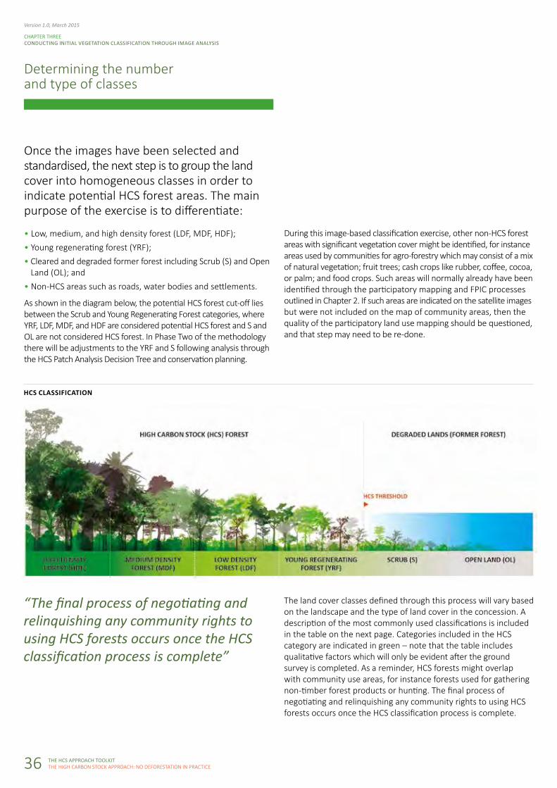
Once the images have been selected and standardised, the next step is to group the land cover into homogeneous classes in order to indicate potential HCS forest areas. The main purpose of the exercise is to differentiate:

• Low, medium, and high density forest (LDF, MDF, HDF);

• Young regenerating forest (YRF);

• Cleared and degraded former forest including Scrub (S) and Open Land (OL); and

• Non-HCS areas such as roads, water bodies and settlements.

As shown in the diagram below, the potential HCS forest cut-off lies between the Scrub and Young Regenerating Forest categories, where YRF, LDF, MDF, and HDF are considered potential HCS forest and S and OL are not considered HCS forest. In Phase Two of the methodology there will be adjustments to the YRF and S following analysis through the HCS Patch Analysis Decision Tree and conservation planning.

During this image-based classification exercise, other non-HCS forest areas with significant vegetation cover might be identified, for instance areas used by communities for agro-forestry which may consist of a mix of natural vegetation; fruit trees; cash crops like rubber, coffee, cocoa, or palm; and food crops. Such areas will normally already have been identified through the participatory mapping and FPIC processes outlined in Chapter 2. If such areas are indicated on the satellite images but were not included on the map of community areas, then the quality of the participatory land use mapping should be questioned, and that step may need to be re-done.

The land cover classes defined through this process will vary based on the landscape and the type of land cover in the concession. A description of the most commonly used classifications is included in the table on the next page. Categories included in the HCS category are indicated in green – note that the table includes qualitative factors which will only be evident after the ground survey is completed. As a reminder, HCS forests might overlap with community use areas, for instance forests used for gathering non-timber forest products or hunting. The final process of negotiating and relinquishing any community rights to using HCS forests occurs once the HCS classification process is complete.





Where single species or near-single species forests are identifiable and mappable, for instance Gelam (Melaleuca spp.) in Indonesia, consideration should be given as to whether the area should be treated as a separate (non – standard) vegetation cover class. If the decision is made to separate a single species area out, the usual HCS approach of stratifying the vegetation of the area into high and low carbon stock classes still applies.

It should be noted that as the Simple Ratio (SR) dynamic range is stretched in favour of high biomass conditions such as forested regions and compressed in low biomass condition, areas of natural regrowth and natural forests could be detected using this method. Moreover, Sentinel-1 Microwave data could also be included to detect the natural forest and natural regrowth regions, as the stand dynamic structure are different and could be inferred from the surface roughness.

TABLE: GENERIC LAND COVER CATEGORIES

VEGETATION COVER DESCRIPTION CATEGORIES

HDF, MDF, LDF High Density Forest, Medium Density Forest, and Low Density Forest

Closed canopy natural forest ranging from high density to low

density forest. Inventory data indicates presence of trees with

diameter > 30cm and dominance of climax species.

YRF Young Regenerating Forest

Highly disturbed forest or forest areas regenerating to their

original structure. Diameter distribution dominated by trees

10-30cm and with higher frequency of pioneer species

compared to LDF. This land cover class may contain small

areas of smallholder agriculture.

Note: Abandoned plantations with less than 50% of basal

area consisting of planted trees could fall in this category

or above. Concentrations >50% of basal area would not be

considered HCS forest but rather plantations and should be

classified separately.

S Scrub

Land areas that were once forest but have been cleared

in the recent past. Dominated by low scrub with limited

canopy closure. Includes areas of tall grass and fern with

scattered pioneer tree species.

Occasional patches of older forest may be found within

this category.

OL Open Land

Recently cleared land with mostly grass or crops.

Few woody plants.

EXAMPLES OF OTHER NON-HCS LAND COVER CATEGORIES

FP Forest Plantation

Large area of planted trees (e.g. rubber, Acacia).

AGRI Agriculture Estates

For instance, large scale oil palm estates overlapping

with concession areas

MINE Mining Area

These can be further differentiated between licensed mining

areas and overflow, unregulated/illegal mining areas

SH Smallholder Agriculture and Use

These areas can be further differentiated among mixed

forest gardens/agroforestry systems which could potentially

serve as wildlife corridors, swidden/rotational gardening

systems for subsistence food production, etc.

(Other) Water bodies such as rivers and lakes.

Built-up areas, settlements, roads, etc.

All photos: Courtesy USGS ©




Approaches to classification

“The selection of the method used to interpret images is generally determined by the level of the interpreter’s expertise and familiarity with the particular landscape”

Once the images have been selected and refined, the land cover is grouped into relatively homogenous classes described above in order to delineate HCS forest from non-HCS. The process primarily consists of analysing the satellite images using Remote Sensing and Geographic Information Systems (GIS) software, which provide tools for land cover interpretation. Several software packages provide the tools to support the land cover classification, including Erdas Imagine, ENVI, ESRI Image Analysis and OpenSource software (Quantum GIS).

Land cover classification is applied for several reasons:

1. It allows the identification of different land cover classes with various forest and non-forest conditions that can be captured in image analysis (e.g. colour, canopy closure and roughness of the canopy layer).

2. The condition of the forest is often (but not always) correlated with forest carbon stock and biodiversity. For example, dense well-stocked forest is usually associated with high carbon stocks (and also commonly higher biodiversity) than degraded, low stocked forest.

3. Separating the land cover into classes allows for more efficient sample design for the ground survey (see Chapter 4), and a simpler review of the results of forest inventory and aerial survey.

HCS studies generally use a combination of several methodological phases to ensure accurate representation of the land cover, namely pixel-based analysis using unsupervised and supervised methods, as well as visual methods in other phases. Regardless of the image classification techniques applied, local field knowledge of land use, land covers, forest types and its species composition, agricultural crop types, and phenology of vegetation in relation to the spectral signature of the selected dataset of images is essential.

The selection of the method used to interpret images is generally determined by the level of the interpreter’s expertise and familiarity with the particular landscape and the land cover area being analysed. For example, if the interpreter has sufficient understanding of sophisticated remote sensing techniques and good knowledge of the sample area, it is recommended to use the supervised classification technique and/or hierarchical decision tree classifier using tools similar to Knowledge Engineer and Knowledge Classifier. For an area with no pre-existing land cover information the interpreter or the analyst may initiate the analysis using the unsupervised classification technique in order to see the spectrally similar and spatially contiguous spatial objects or phenomena.

In general, unsupervised classification, supervised classification techniques and hierarchical decision trees classification will be complementary to determine the classes of land cover in the study area.





Unsupervised classification

Unsupervised classification uses image processing software to group pixels by general characteristics without using any pre-determined sample class. The unsupervised classification applies K-mean image segmentation algorithm or an ISODATA (Iterative Self-Organising Data Analysis) algorithm to determine which pixels are spectrally similar to other pixels and groups them into various homogeneous classes. The user can specify which algorithm the software will use and the desired number of output classes, but otherwise does not intervene in the classification process. However, the user must have knowledge of the area being classified, as the groupings of pixels with common characteristics produced by the unsupervised classification have to be related to actual features on the ground (such as wetlands, developed areas, coniferous forests, etc.)

The classes that result from unsupervised classification are spectral classes. Because these are based solely on the natural grouping in the image values, the identity of the spectral classes will not be initially known. The analyst must compare the classified spectral classes with some form of reference data such as existing maps or field visits to determine the identity and informational value or information classes of the spectral classes.

Once the analyst has determined spectrally separable classes and defined their informational utility, the spectral classes can be aggregated into the smaller set of categories desired by the analyst. Sometimes, the analysts may find that several spectral classes relate to more than one information category. For instance, spectral class 3 could be found to correspond to Young Generation Forest in some locations and Low Density Forest in others. Likewise, Spectral class 6 could include both Medium Density Forest and High Density Forest. This means that these information categories are spectrally similar and cannot be differentiated in a given data set. In this case, the analyst might consider including additional bands to the given data set, as discussed earlier.

Overall, the quality of an unsupervised classification will depend on the analyst’s understanding of the concepts behind the classifier available and knowledge about the land cover types under analysis. When using unsupervised classification in the HCS process, normally 16 classes will be enough to determine the forest and non-forest classes, which are then combined with vegetation cover, and can be a reference to locate the field plots (see Chapter 4).





Supervised classification

“Supervised classification is based on the concept that a user can select sample pixels in an image that are representative of specific classes, this can then become references for the classification of all other pixels in the image”

Supervised classification is based on the concept that a user can select sample pixels in an image that are representative of specific classes and then direct the image processing software to use these training sites as references for the classification of all other pixels in the image. Training sites (also known as testing sets or input classes) are selected based on the knowledge of the user. The user also sets the bounds for how similar other pixels must be to group them together. These bounds are often set based on the spectral characteristics of the training area, plus or minus a certain increment (often based on “brightness” or strength of reflection in specific spectral bands). The user also designates the number of classes into which the image is classified.

Three basic steps are involved in a typical supervised classification procedure:

1. In the training stage, the analyst identifies representative training areas and develops a numerical description of the spectral attributes of each land cover type of interest in the scene.

2. In the classification stage, each pixel in the image data set is categorised into the land cover class it closely resembles. If the pixel is insufficiently similar to any training data set, it is usually classified or labelled unknown.

3. After the entire data set has been categorised, the results are presented in the output stage. The classified output becomes a GIS input.

Each of these steps is described in detail on the following pages.

Training StageThe overall objective of the training stage is to assemble a set of statistics that describes the spectral response pattern for each land cover type to be classified in an image. It is important to note that all spectral classes constituting each information class must be adequately represented in the training set statistics used to classify an image. It is uncommon to acquire data from 100 or more training areas to adequately represent the spectral variability in an image. A histogram output of each training area is particularly important when a maximum likelihood classifier is used, since it provides a visual check on the normality of the spectral response distribution. Liliesand and Kiefer’s Remote Sensing and Image Interpretation (Fifth Edition, 2004) provides detailed information and examples on how to identify statistically valid training areas.

The training area sample section and evaluation of training sample statistics is time consuming, but is an important step for good quality classification. The analyst should spend a good amount of time to create statistically representative and statistically separable training samples which present the information classes. A classification error matrix (described later in this chapter) can be created on the training sets of pixels and the results of supervised classification.

Photo: Courtesy USGS ©




Classification stageWhile many techniques could be used for the supervised classification stage, this toolkit focuses in detail on the Gaussian Maximum Likelihood Classifier1 and also outlines briefly the use of decision trees for hierarchical supervised classification.

The Gaussian Maximum Likelihood Classifier quantitatively evaluates both the variance and covariance of the category response patterns (from training sample statistics) when classifying an unknown pixel. An assumption is made that the distribution of the cloud points forming the category training data is Gaussian, i.e. normally distributed. Under this assumption, the distribution of a category response pattern can be completely described by the mean vector and the co-variance matrix. Given these parameters, the classifier computes the statistical probability of a given pixel value being a member of a particular land cover class or HCS classes. After evaluating the probability in each category, the pixel would be assigned to the most likely class (with the highest probability value) or be labelled ‘unknown’ if the probability values are all below a threshold set by the analyst.

“Many analysts use a combination of supervised and unsupervised classification methods to develop final analyses and classifications for the indicative maps”

1. Pages 271-277 of Resource Management Information Systems: Remote Sensing, GIS and Modelling (second edition) by Keith R. McCloy provide more details on Maximum Likelihood Classification.

An extension of the maximum likelihood approach is the Bayesian classification, which applies two weighted factors to the probability estimate. First, the analyst determines the “a priori probability” or the anticipated likelihood of occurrence for each class in a given scene or image. Second, a weight associated with the cost of misclassification is applied to each class. Together, these factors act to minimise the cost of misclassifications, resulting in a theoretically optimum classification. In practice, most maximum likelihood classification is performed assuming equal probability of occurrence and cost of misclassification for all classes.

Maximum likelihood classification is computationally intensive to classify each pixel especially when either a large number of spectral bands are involved or a large number of spectral classes must be differentiated, but modern multi-core computer processors process the classification fairly quickly. Another means of optimising the maximum likelihood classification is to use Principle Components (PC1, PC2 and PC3) instead of original channels to perform the classification.

An alternative to Maximum Likelihood Classifier is the use of decision trees, which apply a stratified or layered classification to simplify the classification computations and maintain classification accuracy. These classifiers are applied in a series of steps, with certain classes being separated during each step in the simplest manner possible. For example, water could be separated from near infrared band by a simple threshold value. Certain classes may require the combination of two or three bands for categorisation using simpler classification algorithm such as Minimum Distance to Mean Classifier or Parallelepiped Classifier. The use of more bands or Maximum Likelihood Classifier would only be applied for those land cover categories where residual ambiguity exists between overlapping classes in the measurement space. Finally, multinomial logical regression could be applied with training sampling statistics to derive the probability of each pixel to the information classes instead of using Maximum Likelihood Classification.

Many analysts use a combination of supervised and unsupervised classification methods to develop final analyses and classifications for the indicative maps.

Case study: West Kalimantan

In the following case example from West Kalimantan, Indonesia, Landsat 8 satellite images processed with ArcGIS 10.1 with Images Analysis extension were used to classify the land cover. The satellite images were first pre-processed as needed to produce the image of the AOI to the right.

With the existing tools in the image processing software, six training areas were selected, representing the six HCS land cover classes as illustrated in the middle image.

After the training samples were deemed sufficient and representative, a supervised classification using maximum likelihood classification approach was run through the processing software. The resulting interim vegetation map based on image analysis is shown in the bottom image.

Publication date March 2015



THE PHASES OF VISUAL VEGETATION STRATIFICATION




An advanced visual classification or manual digitisation process may be carried out by an experienced analyst with excellent knowledge of the land cover conditions in the area. The analyst is able to determine each land cover class through on-screen analysis of satellite images. Images are commonly enhanced to aid identification of classes. The interpreter must have the knowledge of interpretation keys of the land cover of the study area, integrity value, professional and field experience of the study area.

Visual classification is used after the image has been calibrated and standardised where multiple images in a mosaic are being used. When used as a standalone technique, visual classification is typically the most accurate where the user knows the area well. However, this accuracy comes at a cost, as this technique requires a lot of time-consuming digitising. It can also be biased. It should therefore only be used as a stand-alone process with high-resolution image data and where the user knows the area well.

Alternatively, visual classification can also be used to complement both supervised and unsupervised processes, as these can generate an error or bias, especially in areas with inadequate image quality due to fog, smoke, topographic shadows, cloud shadows or clouds. This error or bias can be minimised through a visual quality control by the interpreter. For areas with incorrect interpretation, corrections are done to match known conditions. In this phase, unsupervised or supervised interpretation results (if applicable) are combined with other elements such as information of soil type and rainfall. An understanding of site conditions becomes the key to generating good and accurate classification. Thus the more site-specific information an interpreter has, the less the bias of error will be.

The phases of visual vegetation stratification are presented in the diagram right.

The additional numerical information such as temperature, rainfall, humidity, solar radiation, wind speed grids, digital elevation models and digital terrain models could be added as the additional bands for classification only if these data provide value-added information to separate between spectral classes. The additional categorical information such as soil types, geology, geomorphology and vegetation locations could be applied to refine the interpretation without bias.

For HCS studies, the authors recommend that visual stratification is not used by remote sensing practitioners until considerable experience is gained from trials of the HCS methodology using supervised or unsupervised classification in combination with the field analysis laid out in the next chapter.

Visual classification

THE PHASES OF VISUAL VEGETATION STRATIFICATION

Onscreen digi�sa�on for delinea�on of vegeta�on

class limits (six vegeta�on classes)

Quality controlreclassifica�on

Supervised or unsupervised classifica�on

Accuracy assessment

Image pre-processing and transforma�on

Satellite images

Physical informa�on• Soil type• Climate

• Ecosystem

Site informa�on• Vegeta�on loca�on

• Vegeta�on condi�on • Vegeta�on structure, etc.

“An understanding of site conditions becomes the key to generating good and accurate classification. Thus the more site-specific information an interpreter has, the less the bias of error will be”

ERROR MATRIX BASED ON TRAINING SAMPLE DATA SET




Accuracy assessment of classified image

This section outlines the accuracy assessment to be undertaken to check the classification. For further information on accuracy assessments, Remote Sensing Thematic Accuracy Assessment: A Compendium (1994) by ASPRS and Assessing the Accuracy of Remotely Sensed Data: Principle and Practices (Congalton and Green, 1999) are excellent references.

Classification error matrix based on training sample data setPreparing a classification error matrix, confusion matrix or contingency table is a common method of expressing classification accuracy. Error matrices compare, on a category-by-category basis, the relation between known reference data (ground truth) and the corresponding results of image classification.

The table below is an example of error matrix based on training samples and classified result, from Liliesand and Kiefer (2004). It provides an example of how well a classification has categorised a representative subset of pixels used in the training process of a supervised classification. This matrix stems from classifying the sample classified into the proper land cover categories are located along the major diagonal (yellow highlighted) of the error matrix. All non-diagonal elements of the matrix represent error of omission (exclusion) or error of commission (inclusion).

The omission error corresponds to non-diagonal COLUMN elements, e.g. 16 pixels that have been classified as “S” for sand were omitted from the category. The producer’s accuracies are calculated by dividing the number of correctly classified pixels in each category (on the major diagonal) by the number of training sets pixels used for that category (the column total). The producer’s accuracy ranges from 51% to 100% in this case, and is a measure of omission error and indicates how well training set pixels of the given cover type are classified.

Commission errors are represented by non-diagonal row elements, for instance 38 urban (U) and 79 hay (H) pixels were improperly included in the Corn (C) category. The user accuracies are calculated by dividing the number of correctly classified pixels by the total number of pixels that were classified in that category (the row total). The user’s accuracy is a measure of commissioning error and indicates the probability that a pixel classified into a given category actually represents that category on the ground. The user’s accuracy in this case ranges from 72% to 99%.

Overall accuracy is calculated by dividing the total number of correctly classified pixels (the sum of elements along the major diagonal) by the total number of reference pixels. Overall accuracy in the example contingency table is 84%.

It is important to note that the example error matrix is based on training data, and such procedures only indicate how well the statistics extracted from these areas can be used to categorise the same areas. If the results are good, it means nothing more than that the training areas are homogeneous, the training classes are spectrally separable, and that the classification strategy being employed works well in the training area. It indicates little about how the classifier performs elsewhere in the scene. Training area accuracies should not be used as an indication of overall accuracy.

Training Set Data (Known Cover Types) W S F U C H Row TotalClassification dataW 480 0 5 0 0 0 485S 0 52 0 20 0 0 72F 0 0 313 40 0 0 353 U 0 16 0 126 0 0 142C 0 0 0 38 342 79 459H 0 0 38 246 60 359 481Column Total 480 68 356 248 402 438 1992

Overall accuracy = (480 + 52 + 313 +126 + 342 +359) / 1992 = 84%

Producer’s Accuracy:W = 480/480 = 100%S = 52/68 = 76%F = 313/356 = 88%U = 126/248 = 51%C = 342/402 = 85%H = 359/438 = 82%

User’s Accuracy: W = 480/485 = 99%S = 52/72 = 72% F = 313/353 = 87% U = 126/142 = 89% C = 342/459 = 74% H = 359/481 = 75%

ERROR MATRIX BASED ON TEST PIXELS




Sampling consideration of test areasTo assess the accuracies of classification for the scene, representative test areas with uniform land cover should be selected. The test areas could be selected through a random, stratified random or systematic sampling framework. Test areas could be selected during the training sample selection stage, setting aside some training samples as the test areas which will not be used as part of the training sample sets. The appropriate sampling unit might be individual pixels, clusters of pixels or polygons. Polygon sampling is the most common approach.

As a broad guideline, a minimum of 50 samples as test areas for each vegetation or land cover category should be included in the error matrix for accuracy assessment of the whole scene classification. If the area is large (e.g. more than a million acres) or the classification has a large number of vegetation or land cover land use categories (more than 12 categories) the minimum number of samples should be increased to 75 to 100 samples per category (Congalton and Green, 1999, p.18). More samples should be selected for the more important categories or more variable categories.

“As a broad guideline, a minimum of 50 samples as test areas for each vegetation or land cover category should be included for accuracy assessment of the whole scene classification”

1. Pages 271-277 of Resource Management Information Systems: Remote Sensing, GIS and Modelling (second edition) by Keith R. McCloy provide more details on Maximum Likelihood Classification.

Evaluating classification error matrix based on test areas or test pixelsOnce accuracy data are collected based on test areas (either in the form of pixels, cluster of pixels or polygons) and summarised in an error matrix, they are normally subject to detailed interpretation and further statistical analyses. The following error matrix was created based on randomly selected test pixels, again from Liliesand and Kiefer (2004):

Overall accuracy is only 65%. If the purpose of mapping is to locate forest (F), the producer accuracy is quite good at 84%. We may conclude that although the overall accuracy was poor (65%), it is adequate for the purpose of mapping forests. The problem with this conclusion is that the user’s accuracy for forest is only 60%. That is, even though 84% of the forested areas have been correctly identified as forest, only 60% of the areas identified as forest within the classification are truly of that category.The user of this classification would find that an area identified as forest from the classification process will prove to be forest on a site visit only 60% of the time. A more careful inspection of the error matrix shows that there is significant confusion between forest and urban (U). In this example matrix, the only reliable category associated with this classification from both a producer’s and a user’s perspective is water (W).

Reference Data for Randomly Selected Test Pixels W S F U C H Row TotalClassification dataW 226 0 0 12 0 1 239S 0 216 0 92 1 0 309F 3 0 360 228 3 5 599 U 2 108 2 397 8 4 521C 1 4 48 132 190 78 453H 1 0 19 84 36 219 359Column Total 233 238 429 945 238 307 2480

Overall accuracy = (226 + 216 + 360 + 397 + 190 + 219) / 2480 = 65%

Omission Error:W = 226/233 = 97%S = 216/328 = 66%F = 360/429 = 84%U = 397/945 = 42%C = 190/238 = 80%H = 219/307 = 71%

Commission Error: W = 226/239 = 94%S = 216/309 = 70% F = 360/599 = 60% U = 397/521 = 76% C = 190/453 = 42% H = 219/359 = 75%




Khat statistics

The Khat statistic is a measure of the difference between the actual agreement between reference data and an automated classifier and the chance agreement between the reference data and a random classifier. It is conceptually defined as follows:

Khat = (observed frequency – chance agreement) / (1 – chance agreement)

This statistic serves as an indicator of the extent to which the percentage correct values of an error matrix are due to “true” agreement versus “chance” agreement. As the true agreement (observed) approaches to 1 and chance agreement approaches 0, Khat approaches to 1. In reality, Khat value ranges between 0 and 1. For example a Khat value of 0.67 can be interpreted as an indication that an observed classification is that 67% better than one resulting from chance. A Khat value of zero suggests that a given classification is no better than a random assignment of pixels. If the chance agreement is larger, Khat could be negative values – an indication of very poor classification performance.

The Khat value is computed as follows:

Khat =

Where:

r = number of rows in the error matrix

xii = number of observations in row i and column i (on the major diagonal)

xi+ = total of observations in row i (shown as marginal total to right of the matrix)

x+i = total of observations in column i (shown as marginal total at the bottom of the matrix

N = total number of observations included in the matrix

For the error matrix shown above, the Khat value is calculated as such:

∑i=1xii = 226 + 216 + 360 + 397 +190 + 219 = 1608

∑i=1(xi+*x+i) = (239 * 233) + (309 * 328) + (599 * 429) + (521 * 945) + (453 * 238) + (359 * 307) = 1,124, 382

Khat = (2480 (1608) - 1124382) 24802 - 1124382)

Khat = 0.57

The Khatvalue (0.57) is lower than the overall accuracy (0.67) computed earlier. As a reminder, the overall accuracy only includes the data along the major diagonal and excludes the errors of omission and commission. Khat incorporates the diagonal elements and the non-diagonal elements of the error matrix as the product of the row and column marginal. One of the advantages of computing Khat statistics is the ability to use this value as the basis for determining the statistical significance of any given matrix or the differences among the matrices.

Normally it is desirable to compute and analyse both the overall accuracy and Khat statistics. The analyst should provide the error matrix based on the training sample, the error matrix of test areas or test pixels, overall accuracy, producer’s accuracy, user’s accuracy and Khat statistics of provided error matrices for the quality assurance of HCS classifications.

Photo top: Courtesy USGS © Photos bottom: Courtesy TFT ©




Quality control, finalising the initial land cover classification and next steps

The steps for finalising the initial land cover classification are described below.

Raster to vector conversionConvert the raster image to a vector format to make editing of land cover class boundaries easier.

Elimination of small patchesElimination of small polygons (4 pixels and smaller) is done by merging them with the closest larger polygon with similar properties; elimination of the sliver polygons (elongated polygons) is done by using the area/perimeter ratio. Minimum mapping area or units should be defined in order to remove polygon patches.

Incorporating other land use informationIn finalising the initial map, information regarding current land use is incorporated into the analysis. For example, already-developed land is removed from potential HCS forest areas.

Editing the vegetation classes using composite 654 band-Landsat 8 (LDCM) imageIn this step, the land cover class vector data is overlaid on a composite Landsat Image (654 band) and a visual comparison is made, with editing as required.

QC vector editing results reclassified into HCS classesThe land cover strata are reclassified into the six standard HCS vegetation classes: OL, S, YRF, LDF, MDF, and HDF.

Edge matching of vector dataIf more than one Landsat image is used, the resulting classification vector data needs to be combined using the edge matching process.

Conduct aerial survey if possibleAerial surveys should be conducted over major contiguous areas of natural forest where possible. A geo-database can then be created to enable photo viewing in GIS. This enables easy cross-checking of land cover classification.

Prepare draft land cover mapA draft land cover map, categorised by the various classes identified in the process outlined above, is then prepared for use in planning and implementation of field work, including the aerial survey and the forest inventory.

“The next step is to compare the results of the image interpretation with measurements taken in the field, allowing us to calculate approximate carbon values for each class”

Next steps

The next stage in the HCS classification process is to test the accuracy of the interpretation results, as the accuracy will strongly influence the user’s trust in the data and methods of analysis. The initial classification accuracy report of classification of satellite image for HCS vegetation stratification from the perspective of contingency table (error matrix or confusion table), producer’s accuracy, user’s accuracy, overall accuracy, Khat statistics and interpretation of accuracy assessment report have been discussed here. The next step is to compare the results of the image interpretation with measurements taken in the field. This also allows us to calculate approximate carbon values for each class.

The next chapter will explain how to collect sample field data required to estimate the above-ground biomass and carbon stock, assign average carbon levels to each category (while noting that the purpose is not to calculate an exact carbon number but rather to differentiate types of land cover through estimated carbon values), and further refine the classification in order to create the lland cover map in which potential HCS forest areas are delineated.




Appendices

Sate

llite

Nam

e

Ove

rvie

w

Spati

al re

solu

tion

(m)

Tem

pora

l res

oluti

on

Imag

e ca

ptur

e da

tes

Cost

per

scen

e (U

SD)

Avai

labl

e ba

nds

Size

of i

mag

es

Com

men

ts

Landsat 8

ALOS (AVNIR-2, PRISM)

IKONOS

http://landsat.usgs.gov/landsat8.php

http://www.alos-restec.jp/en/

http://geofuse.geoeye.com/landing/

http://glcf.umd.edu/data/

30m

10m

4m

16 days

46 days

14 days

Feb 2013 – Present

Jan 2006 – May 2011

2000 –

Free

$16-56/Km2

11 Bands:1. 0.433–0.453 30 m

2. 0.450–0.515 30 m3. 0.525–0.600 30 m4. 0.630–0.680 30 m5. 0.845–0.885 30 m6. 1.560–1.660 30 m

1270 MHz (L-band), Polarization HH+VV

1 (Blue)2 (Green)3 (Red)4 (Near-IR)

185km by 180km

14km by 14km

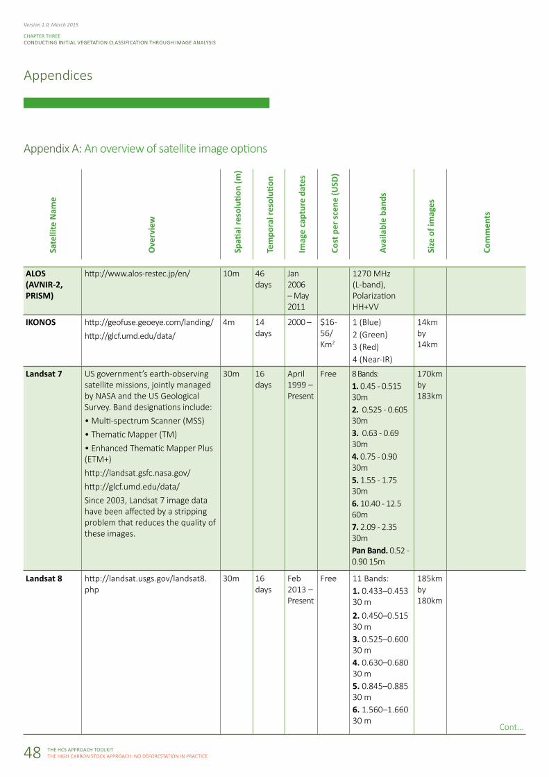
Appendix A: An overview of satellite image options

Landsat 7 US government’s earth-observing satellite missions, jointly managed by NASA and the US Geological Survey. Band designations include:

• Multi-spectrum Scanner (MSS)

• Thematic Mapper (TM)

• Enhanced Thematic Mapper Plus (ETM+)

http://landsat.gsfc.nasa.gov/


Since 2003, Landsat 7 image data have been affected by a stripping problem that reduces the quality of these images.

30m 16 days

April 1999 – Present

Free 8 Bands:1. 0.45 - 0.515 30m2. 0.525 - 0.605 30m3. 0.63 - 0.69 30m4. 0.75 - 0.90 30m5. 1.55 - 1.75 30m6. 10.40 - 12.5 60m 7. 2.09 - 2.35 30mPan Band. 0.52 - 0.90 15m

170km by 183km

Cont...

http://landsat.usgs.gov/landsat8.php




Sate

llite

Nam

e

Ove

rvie

w

Spati

al re

solu

tion

(m)

Tem

pora

l res

oluti

on

Imag

e ca

ptur

e da

tes

Cost

per

scen

e (U

SD)

Avai

labl

e ba

nds

Size

of i

mag

es

Com

men

ts

Landsat 8 Cont...

Quickbird

Radarsat 2

http://www.digitalglobe.com


http://www.asc-csa.gc.ca/eng/satellites/radarsat2/

Although radar data does not have infrared band, it has other important backscattering information. It is also able to penetrate through cloud cover and operate day and night. However, the data processing is more tedious as compared to optical data.

2.4m

3m – 100m*

4 days

24 days

2001 – Present

Dec 2007 - Present

$5,000 -11, 500/ scene $16-45 /km2

$3,300 – $7,700

7. 2.100–2.300 30 m8. 0.500–0.680 15 m9. 1.360–1.390 30 m10. 10.6-11.2 100 m11. 11.5-12.5 100 m

Multispectral1 = Blue2 = Green3 = Red4 = NIR• Panchromatic

Pan

C Band SAR Antenna-Transmit & Receive Channel: 5405.0000 MHz (assigned bandwidth 100,540 kHz)

16.5km x 16.5km

Radar data lacks an infrared band and therefore requires additional care to classify different vegetation classes.


RapidEye http://www.rapideye.de/ 5m 5.5 days

2009 $1.5 / km2

1. 440 – 510 nm (Blue)2. 520 – 590 nm (Green)3. 630 – 685 nm (Red)4. 690 – 730 nm (Red Edge)5. 760 – 850 nm (Near IR)

25km x 25km

Radar data lacks an infrared band and therefore requires additional care to classify different vegetation classes.

Cont...

http://www.asc-csa.gc.ca/eng/satellites/radarsat2/




Appendices

Sate

llite

Nam

e

Ove

rvie

w

Spati

al re

solu

tion

(m)

Tem

pora

l res

oluti

on

Imag

e ca

ptur

e da

tes

Cost

per

scen

e (U

SD)

Avai

labl

e ba

nds

Size

of i

mag

es

Com

men

ts


Worldview-1

Worldview-2

http://www.alos-restec.jp/en/

http://www.satimagingcorp.com/satellite-sensors/worldview-2/

0.50 meter GSD at Nadir

0.55 meter GSD at 20˚ off-nadir

Ground Sample Distance (GSD) Panchr- omatic: 0.46m GSD at Nadir, 0.52m GSD at 20° Off- Nadir

Multisp- ectral: 1.84m GSD at

1.7 days at 1 meter GSD or Less

5.9 days at 20˚ off-nadir or less 0.51 meter GSD

1 m GSD: <1.0 day

4.5 days at 20° off-nadir or less

Sept 2007 to Present

August 2014 to Present

Panchromatic

Panchromatic @ 450-800nm8 Multispectral bands @ 400 – 1040 nm8 SWIR bands @ 1195 – 2365 nm12 CAVIS Bands @405 – 2245 nm

17.6 km at Nadir

17.6 km X 14 km or 246,4 km2 at Nadir

At nadir: 13.1 km

Maximum view Angle or Accessible Ground Swath

60km by 110km

or

30km by 110km Stereo Image acquisition

Max Conti-guous Area Collected in a Single Pass (30° off-nadir angle)

Mono: 66.5km x 112km (5 strips)

Stereo: 26.6km x 112km (2 pairs)

SPOT-5 Satellite network run by the French Space Agency.

http://www.satimagingcorp.com/satellite-sensors/other-satellite-sensors/spot-5/

2.5m to 10m

24 days

1986 - Present

$1,500 - $2,500

5 bands:Panchromatic (450 – 745 nm)Blue (450-525 nm)Green (530 – 590 nm)Red (625 - 695 nm)Near-infrared (760 – 890 nm)

60km by 60km

Cont...

http://www.satimagingcorp.com/satellite-sensors/other-satellitesensors/spot-5/





Sate

llite

Nam

e

Ove

rvie

w

Spati

al re

solu

tion

(m)

Tem

pora

l res

oluti

on

Imag

e ca

ptur

e da

tes

Cost

per

scen

e (U

SD)

Avai

labl

e ba

nds

Size

of i

mag

es

Com

men

ts


Worldview-2 Cont...

Worldview-3 http://www.satimagingcorp.com/satellite-sensors/worldview-3/

Nadir, 2.4m GSD at 20° Off-Nadir

Pan. Nadir: 0.31m GSD at Nadir

0.34 m at 20° Off- Nadir

Multi- spectral Nadir: 1.24m at Nadir, 1.38 m at 20° Off-Nadir

SWIR Nadir: 3.70m at Nadir, 4.10m at 20° Off-Nadir

CAVIS Nadir: 30.00 m

1m GSD: <1.0 day4.5 days at 20° off-nadir or less

August 2014 – Present

Panchromatic @ 450-800nm8 Multispectral bands @ 400 – 1040 nm

8 SWIR bands @ 1195 – 2365 nm

12 CAVIS Bands @405 – 2245 nm

At nadir: 13.1km

Max Conti-guous Area Collected in a Single Pass (30° off-nadir angle)

Mono: 66.5km x 112km (5 strips)

Stereo: 26.6km x 112km (2 pairs)

Cont...





Appendices

Sens

or

Web

site

Spati

al re

solu

tion

Tem

pora

l res

oluti

on

Imag

e ca

ptur

e da

tes

Cost

of i

mag

e

Avai

labl

e ba

nds

Swatt

h

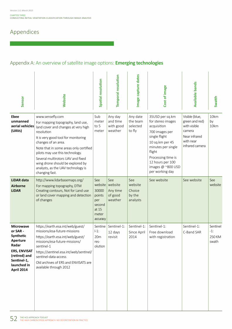
Appendix A: An overview of satellite image options: Emerging technologies

Ebee unmanned aerial vehicles (UAVs)

LiDAR dataAirborne LiDAR

Microwave or SAR - Synthetic Aperture RadarERS, ENVISAT (retired) and Sentinel-1, launched in April 2014

www.sensefly.com

For mapping topography, land use, land cover and changes at very high resolution

It is very good tool for monitoring changes of an area.

Note that in some areas only certified pilots may use this technology.

Several multirotors UAV and fixed wing drone should be explored by analysts, as the UAV technology is changing fast.

http://www.lidarbasemaps.org/

For mapping topography, DTM Creating contours, Not for Land use or land cover mapping and detection of changes

https://earth.esa.int/web/guest/missions/esa-future-missions

https://earth.esa.int/web/guest/missions/esa-future-missions/sentinel-1

https://sentinel.esa.int/web/sentinel/sentinel-data-access

Old archives of ERS and ENVISATS are available through 2012

Sub meter to 5 meter

See website

30000 points per second at 15 meter accuracy

Sentine l-1:

20m resolution

Any day and time with good weather

See website

Any time of good weather

Sentinel-1:

12 days revisit

Any date the team selected to fly

See website

Choice by the analysts

Sentinel-1:

Since April 2014

35USD per sq.km for stereo images acquisition

700 images per single flight

10 sq.km per 45 minutes per single flight

Processing time is 12 hours per 100 images @ ~800 USD per working day

See website

Sentinel-1:

Free download with registration

Visible (blue, green and red) with visible camera

Near infrared with near infrared camera

See website

Sentinel-1:

C-Band SAR

10km by 10km

See website

Sentinel -1:

250 KM swath

https://earth.esa.int/web/guest/missions/esa-future-missions

https://earth.esa.int/web/guest/missions/esa-future-missions/sentinel-1

https://sentinel.esa.int/web/sentinel/sentinel-data-access




Kauth and Thomas (1976) produced an orthogonal transformation of the original Landsat MSS data space to a new four dimensional feature space. It was called the Tasseled Cap or Kauth-Thomas transformation. The name ‘Tasselled Cap’ comes from its cap shape in Greenness (as Y) and Brightness (as X) plots. It created four new axes: the soil brightness index (B), greenness vegetation index (G), yellow stuff index (Y) and none such (N). The names attached to the new axes indicate the characteristics the indices were intended to measure.

The coefficients for Landsat MSS are (Kauth et al., 1979):

B = 0.322*MSS1 + 0.603*MSS2 + 0.675*MSS3 + 0.262*MSS4

G= - 0.283*MSS1 -0.660*MSS2 + 0.577*MSS3 + 0.388*MSS4

Y = - 0.899*MSS1 + 0.428*MSS2 + 0.076*MSS3 – 0.041*MSS4

N = - 0.061*MSS1 +0.131*MSS2 - 0.452 * MSS3 + 0.882 * MSS4

Crist and Kauth (1986) derived the visible, near infrared and middle infrared coefficients for transforming Landsat Thematic Mapper (TM) imagery into brightness (B), greenness (G) and wetness (W) variables.

B = 0.2909*TM1 + 0.2493*TM2 + 0.4806*TM3 + 0.5568*TM4 + 0.4438*TM5 + 0.1706*TM7

G = - 0.2728*TM1 – 0.2174*TM2 – 0.5508*TM3 +0.7221*TM4 + 0.0733*TM5 – 0.1648*TM7

W = 0.1446 * TM1 + 0.1761*TM2 +0.3322*TM3 +0.3396*TM4 – 0.6210*TM5 – 0.4186*TM7

Tasseled Cap coefficients for Landsat 7 Enhanced Thematic Mapper Plus (ETM+) are (Huang et al., 2002)

B = 0.3561*TM1 + 0.3972*TM2 + 0.3904*TM3 + 0.6966*TM4 + 0.2286*TM5 + 0.1596*TM7

G = -0.334*TM1 – 0.354*TM2 -0.456*TM3 + 0.6966*TM4 – 0.24*TM5 – 0.263* TM7

W = 0.2626*TM1 + 0.2141*TM2 + 0.0926*TM3 + 0.0656*TM4 – 0.763*TM5 – 0.539*TM7

Fourth = 0.0805*TM1 – 0.050*TM2 + 0.1950*TM3 – 0.133*TM4 + 0.5752*TM5 – 0.777*TM7

Fifth = -0.725*TM1 – 0.020*TM2 + 0.6683*TM3 + 0.0631*TM4 - 0.149*TM5 – 0.027*TM7

Sixth = -0.400*TM1 – 0.817*TM2 + 0.3832*TM3 + 0.0602*TM4 – 0.109*TM5 + 0.0985*TM7

Tasseled Cap coefficients for transformation of Landsat 8 imagery (Baig et al., 2014) are:

B = 0.3029*TM2 + 0.2786*TM3 + 0.4733*TM4 + 0.5599*TM5 + 0.508*TM6 + 0.1872*TM7

G = -0.2941*TM2 – 0.243*TM3 – 0.5424*TM4 + 0.7276*TM5 + 0.0713*TM6 – 0.1608*TM7

W = 0.1511*TM2 + 0.1973*TM3 + 0.3283*TM4 + 0.3407*TM5 - 0.7117*TM6 - 0.4559*TM7

Fourth = -0.8239*TM2 + 0.0849*TM3 + 0.4396*TM4 - 0.058*TM5 + 0.2013*TM6 - 0.2773*TM7

Fifth = -0.3294*TM2 + 0.0557*TM3 + 0.1056*TM4 + 0.1855*TM5 - 0.4349*TM6 + 0.8085*TM7

Sixth = 0.1079*TM2 - 0.9023*TM3 + 0.4119*TM4 + 0.0575*TM5 - 0.0259*TM6 + 0.0252*TM7

Appendix B: Tasseled Cap transformation

version 1.0, march 2015 conducting initial vegetation

Documents