vertex coloring of a graph - İyte...
TRANSCRIPT
VERTEX COLORING OF A GRAPH
A Thesis Submitted tothe Graduate School of Engineering and Sciences of
Izmir Institute of Technologyin Partial Fulfillment of the Requirements for the Degree of
MASTER OF SCIENCE
in Mathematics
byGoksen BACAK
December 2004IZMIR
We approve the thesis of Goksen BACAK
Date of Signature
. . . . . . . . . . . . . . . . . . . . . . . . . . . . . . . . . . . . . . 29 December 2004Asst. Prof. Dr. Unal UFUKTEPESupervisorDepartment of Mathematics
Izmir Institute of Technology
. . . . . . . . . . . . . . . . . . . . . . . . . . . . . . . . . . . . . . 29 December 2004Assoc. Prof. Dr. Alpay KIRLANGICDepartment of MathematicsEge University
. . . . . . . . . . . . . . . . . . . . . . . . . . . . . . . . . . . . . . 29 December 2004Assoc. Prof. Dr. Urfat NURIYEVDepartment of MathematicsEge University
. . . . . . . . . . . . . . . . . . . . . . . . . . . . . . . . . . . . . . 29 December 2004Asst. Prof. Dr. Gamze TANOGLUHead of Department
Izmir Institute of Technology
. . . . . . . . . . . . . . . . . . . . . . . . . . . . . . . . .
Prof. Dr. Semra ULKUHead of the Graduate School
ACKNOWLEDGEMENTS
This thesis could not have been accomplished without many people’s support.
First of all, I would like to express my deepest gratitude to my advisor Asst.Prof.Dr.
Unal Ufuktepe for his guidance, encouragement, patience and above all for being a great
teacher. He was always approachable for any academic / non-academic issues that I faced.
There are some people that they change people’s life positively. But they are very few
and my advisor is one of them.
I would also like to thank Assoc.Prof.Dr. Alpay Kırlangıc and Assoc.Prof.Dr.
Urfat Nuriyev for being on my thesis committee. It was great honor having them both.
I have lucky enough to have the support of my good friends. Life would not have
been the same without my roommates. I owe a lot to my friend, colleague and roommate
Tina Beseri. Our conversations and work together have greatly influenced this thesis. I
would like to thank Ahmet Yantır and Sultan Eylem Toksoy for having shared the same
room with me and for being good colleagues during the last two years.
Finally, I want to thank my family, my parents and my sweet sister, for their love
and support.
ABSTRACT
Vertex coloring is the following optimization problem; given a graph, how many
colors are required to color its vertices in such a way that no two adjacent vertices receive
the same color? The required number of colors is called the chromatic number of G and is
denoted by χ(G). In this thesis, we reviewed the vertex coloring concepts and theorems.
The package ColorG which we have improved has many functions for dealing with graph
coloring. This package uses a heuristic method due to Brelaz to color the graph so that
adjacent vertices have distinct colors.
iv
OZET
Tepe boyama, verilen bir cizgenin komsu tepelerinin farklı renklerle boyanması
kosuluyla gereken en az renk sayısının bulunmasını konu alan bir optimizasyon prob-
lemidir. Gereken en az renk sayısı cizgenin kromatik sayısıdır ve χ(G) ile gosterilir.
Gelistirdigimiz ColorG isimli Mathematica paketin cizgelerin boyanmasıyla ilgili bircok
fonksiyonu vardır. Bu paket cizgelerin boyanması icin Brelaz algoritmasını kullanmak-
tadır.
v
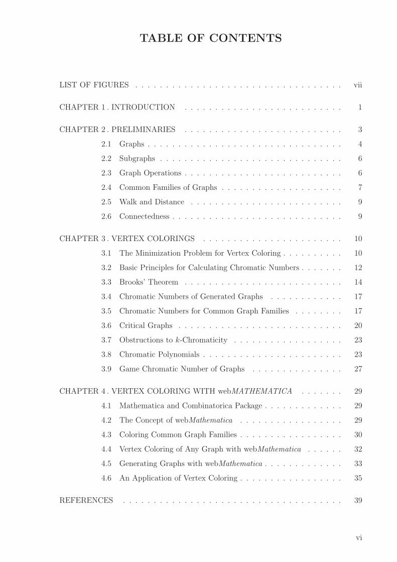
TABLE OF CONTENTS
LIST OF FIGURES . . . . . . . . . . . . . . . . . . . . . . . . . . . . . . . . . . vii
CHAPTER 1 . INTRODUCTION . . . . . . . . . . . . . . . . . . . . . . . . . . 1
CHAPTER 2 . PRELIMINARIES . . . . . . . . . . . . . . . . . . . . . . . . . . 3
2.1 Graphs . . . . . . . . . . . . . . . . . . . . . . . . . . . . . . . . 4
2.2 Subgraphs . . . . . . . . . . . . . . . . . . . . . . . . . . . . . . 6
2.3 Graph Operations . . . . . . . . . . . . . . . . . . . . . . . . . . 6
2.4 Common Families of Graphs . . . . . . . . . . . . . . . . . . . . 7
2.5 Walk and Distance . . . . . . . . . . . . . . . . . . . . . . . . . 9
2.6 Connectedness . . . . . . . . . . . . . . . . . . . . . . . . . . . . 9
CHAPTER 3 . VERTEX COLORINGS . . . . . . . . . . . . . . . . . . . . . . . 10
3.1 The Minimization Problem for Vertex Coloring . . . . . . . . . . 10
3.2 Basic Principles for Calculating Chromatic Numbers . . . . . . . 12
3.3 Brooks’ Theorem . . . . . . . . . . . . . . . . . . . . . . . . . . 14
3.4 Chromatic Numbers of Generated Graphs . . . . . . . . . . . . 17
3.5 Chromatic Numbers for Common Graph Families . . . . . . . . 17
3.6 Critical Graphs . . . . . . . . . . . . . . . . . . . . . . . . . . . 20
3.7 Obstructions to k-Chromaticity . . . . . . . . . . . . . . . . . . 23
3.8 Chromatic Polynomials . . . . . . . . . . . . . . . . . . . . . . . 23
3.9 Game Chromatic Number of Graphs . . . . . . . . . . . . . . . 27
CHAPTER 4 . VERTEX COLORING WITH webMATHEMATICA . . . . . . . 29
4.1 Mathematica and Combinatorica Package . . . . . . . . . . . . . 29
4.2 The Concept of webMathematica . . . . . . . . . . . . . . . . . 29
4.3 Coloring Common Graph Families . . . . . . . . . . . . . . . . . 30
4.4 Vertex Coloring of Any Graph with webMathematica . . . . . . 32
4.5 Generating Graphs with webMathematica . . . . . . . . . . . . . 33
4.6 An Application of Vertex Coloring . . . . . . . . . . . . . . . . . 35
REFERENCES . . . . . . . . . . . . . . . . . . . . . . . . . . . . . . . . . . . . 39
vi
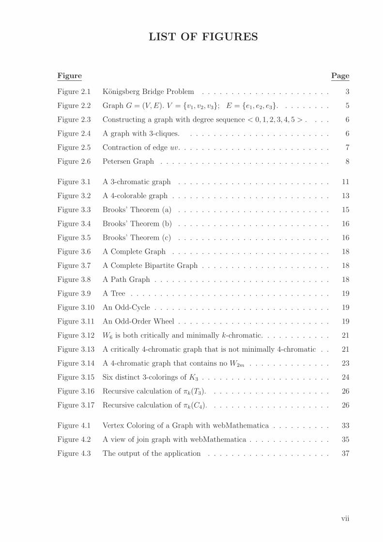
LIST OF FIGURES
Figure Page
Figure 2.1 Konigsberg Bridge Problem . . . . . . . . . . . . . . . . . . . . . . 3
Figure 2.2 Graph G = (V,E). V = {v1, v2, v3}; E = {e1, e2, e3}. . . . . . . . . 5
Figure 2.3 Constructing a graph with degree sequence < 0, 1, 2, 3, 4, 5 > . . . . 6
Figure 2.4 A graph with 3-cliques. . . . . . . . . . . . . . . . . . . . . . . . . 6
Figure 2.5 Contraction of edge uv. . . . . . . . . . . . . . . . . . . . . . . . . . 7
Figure 2.6 Petersen Graph . . . . . . . . . . . . . . . . . . . . . . . . . . . . . 8
Figure 3.1 A 3-chromatic graph . . . . . . . . . . . . . . . . . . . . . . . . . . 11
Figure 3.2 A 4-colorable graph . . . . . . . . . . . . . . . . . . . . . . . . . . . 13
Figure 3.3 Brooks’ Theorem (a) . . . . . . . . . . . . . . . . . . . . . . . . . . 15
Figure 3.4 Brooks’ Theorem (b) . . . . . . . . . . . . . . . . . . . . . . . . . . 16
Figure 3.5 Brooks’ Theorem (c) . . . . . . . . . . . . . . . . . . . . . . . . . . 16
Figure 3.6 A Complete Graph . . . . . . . . . . . . . . . . . . . . . . . . . . . 18
Figure 3.7 A Complete Bipartite Graph . . . . . . . . . . . . . . . . . . . . . . 18
Figure 3.8 A Path Graph . . . . . . . . . . . . . . . . . . . . . . . . . . . . . . 18
Figure 3.9 A Tree . . . . . . . . . . . . . . . . . . . . . . . . . . . . . . . . . . 19
Figure 3.10 An Odd-Cycle . . . . . . . . . . . . . . . . . . . . . . . . . . . . . . 19
Figure 3.11 An Odd-Order Wheel . . . . . . . . . . . . . . . . . . . . . . . . . . 19
Figure 3.12 W6 is both critically and minimally k-chromatic. . . . . . . . . . . . 21
Figure 3.13 A critically 4-chromatic graph that is not minimally 4-chromatic . . 21
Figure 3.14 A 4-chromatic graph that contains no W2m . . . . . . . . . . . . . . 23
Figure 3.15 Six distinct 3-colorings of K3 . . . . . . . . . . . . . . . . . . . . . . 24
Figure 3.16 Recursive calculation of πk(T3). . . . . . . . . . . . . . . . . . . . . 26
Figure 3.17 Recursive calculation of πk(C4). . . . . . . . . . . . . . . . . . . . . 26
Figure 4.1 Vertex Coloring of a Graph with webMathematica . . . . . . . . . . 33
Figure 4.2 A view of join graph with webMathematica . . . . . . . . . . . . . . 35
Figure 4.3 The output of the application . . . . . . . . . . . . . . . . . . . . . 37
vii
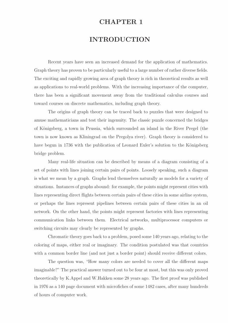
CHAPTER 1
INTRODUCTION
Recent years have seen an increased demand for the application of mathematics.
Graph theory has proven to be particularly useful to a large number of rather diverse fields.
The exciting and rapidly growing area of graph theory is rich in theoretical results as well
as applications to real-world problems. With the increasing importance of the computer,
there has been a significant movement away from the traditional calculus courses and
toward courses on discrete mathematics, including graph theory.
The origins of graph theory can be traced back to puzzles that were designed to
amuse mathematicians and test their ingenuity. The classic puzzle concerned the bridges
of Konigsberg, a town in Prussia, which surrounded an island in the River Pregel (the
town is now known as Kliningrad on the Pregolya river). Graph theory is considered to
have begun in 1736 with the publication of Leonard Euler’s solution to the Konigsberg
bridge problem.
Many real-life situation can be described by means of a diagram consisting of a
set of points with lines joining certain pairs of points. Loosely speaking, such a diagram
is what we mean by a graph. Graphs lend themselves naturally as models for a variety of
situations. Instances of graphs abound: for example, the points might represent cities with
lines representing direct flights between certain pairs of these cities in some airline system,
or perhaps the lines represent pipelines between certain pairs of these cities in an oil
network. On the other hand, the points might represent factories with lines representing
communication links between them. Electrical networks, multiprocessor computers or
switching circuits may clearly be represented by graphs.
Chromatic theory goes back to a problem, posed some 140 years ago, relating to the
coloring of maps, either real or imaginary. The condition postulated was that countries
with a common border line (and not just a border point) should receive different colors.
The question was, “How many colors are needed to cover all the different maps
imaginable?” The practical answer turned out to be four at most, but this was only proved
theoretically by K.Appel and W.Hakken some 28 years ago. The first proof was published
in 1976 as a 140 page document with microfiches of some 1482 cases, after many hundreds
of hours of computer work.
Apart from being an exercise in abstract thinking, what practical application does
this have? The coloring theory brings one immediate application to mind. If you want
to make a timetable for an exam, one common condition is that you cannot have two
papers written by students at the same time if one or more of the students has to write
both papers. If you rephrase the problem correctly it turns out to be a simple coloring
matter. The idea of using the minimum number of colors then translates to, “What is
the minimum number of sessions you need to set up the timetable?”
We begin our study in Chapter 2, by introducing many of the basic concepts that
we shall encounter throughout this thesis. In Chapter 3, we introduce the vertex coloring
problem. In Section 3.1, we define vertex coloring and chromatic number of a graph,
then in Section 3.2 basic principles for calculating chromatic numbers. We present the
proof of Brooks’ Theorem in Section 3.3. Chromatic numbers for generated graphs and
common graph families are given in Section 3.4 and Section 3.5. Then, in Section 3.6 we
give definition of critical graphs and some important theorems about the critical graphs.
Obstructions to k-chromaticity and chromatic polynomials are given in Section 3.7 and
3.8. Finally, in Chapter 4, we describe some web-based interactive examples on vertex
coloring with webMathematica by using our package ColorG.
2
CHAPTER 2
PRELIMINARIES
How can we lay cable at minimum cost to make every telephone reachable from
every other? What is the fastest route from the national capital to each state capital?
How can n jobs be filled by n people with maximum total utility? What is the maximum
flow per unit time from source to sink in a network of pipes? How many layers does a
computer chip need so that wires in the same layer don’t cross? How can the season of
a sports league be scheduled into the minimum number of weeks? In what order should
a travelling salesman visit cities to minimize travel time? Can we color the regions of
every map using four colors so that neighboring regions receive different colors? These
and many other practical problems involve graph theory. In this chapter we will give some
definitions and properties of graphs.
The problem that is often said to have been the birth of graph theory will suggest
our basic definitions of a graph.
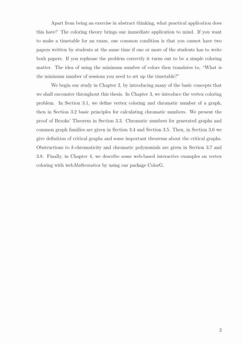
The Konigsberg Bridge Problem
The city of Konigsberg was located on the Pregel river in Prussia. The city occu-
pied two islands plus areas on both blanks. These regions were linked by seven bridges
as shown in the Figure 2.1. The citizens wondered whether they could leave home, cross
every bridge exactly once, and return home. The problem reduces to traversing the figure
on the right, with heavy dots representing land masses and curves representing bridges.
12
3 4
5
6
7
W Y
Z
XX
Y
Z
W
/e6
.e7
.e1
.e3
.e4
.e2
.e5
Figure 2.1: Konigsberg Bridge Problem
The model on the right makes it easy to argue that the desired traversal does not
exist. Each time we enter and leave a land mass, we use two bridges ending at it. We
can also pair the first bridge with the last bridge on the land mass where we begin and
end. Thus existence of the desired traversal requires that each land mass be involved in
an even number of bridges. This necessary condition did not hold in Konigsberg.
2.1 Graphs
A graph is a mathematical structure consisting of two sets V and E. The elements
of V are called vertices and the elements of E are called edges. Each edge is identified
with a pair of vertices. If the edges of a graph G are identified with ordered pairs of
vertices, then G is called a directed graph. Otherwise G is called an undirected graph.
Our discussions in this thesis are concerned with undirected graphs.
We use the symbols v1, v2, v3, ... to represent the vertices and the symbols
e1, e2, e3, ... to represent the edges of a graph. The vertices vi and vj associated with
an edge el are called the end vertices of el. The edge el is then denoted as el = vivj.
Note that while the elements of E are distinct, more than one edge in E may have the
same pair of end vertices. All edges having the same pair of end vertices are called par-
allel or multiple edges. Further, the end vertices of an edge need not be distinct. If
el = vivi, then the edge el is called a self-loop at vertex vi. A graph is called a simple
graph if it has no parallel edges or self-loops. In this thesis we will work with the simple
graphs. A graph G is planar if there exists a drawing of G in the plane in which no two
edges intersect in a point other than a vertex of G.
The cardinality of the vertex set of a graph G is called the order of G and is
commonly denoted by n(G), or more simply by n when the graph under consideration is
clear; while the cardinality of its edge set is the size of G and is often denoted by m(G)
or m. An (n,m) graph has order n and size m. A graph with no edges is called an empty
graph. A graph with no vertices (and hence no edges) is called a null graph.
An edge is said to be incident on its end vertices. Two vertices are adjacent if
they are the end vertices of an edge. The neighborhood of v, N(v), is the set of vertices
adjacent to v. If two edges have a common end vertex, then these edges are said to be
adjacent.
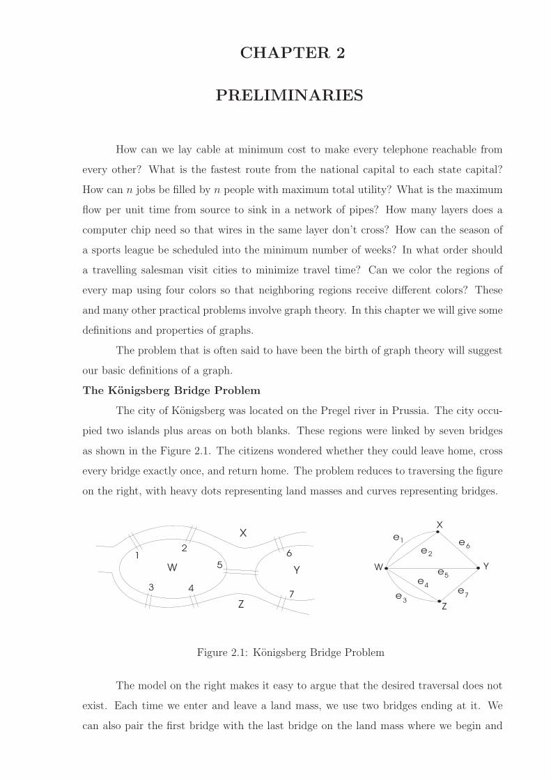
For example, in the Figure 2.2 edge e1 is incident on vertices v1 and v2; v1 and v3
are two adjacent vertices, while e1 and e3 are two adjacent edges.
An independent set of vertices in a graph is a set of mutually non-adjacent
vertices. The independence number of a graph G is the maximum cardinality of an
independent set of vertices. It is denoted by α(G).
4
/v3
/v1
/v2
/e2
/e1 2/e
/e3
Figure 2.2: Graph G = (V,E). V = {v1, v2, v3}; E = {e1, e2, e3}.
The number of edges incident on a vertex vi is called the degree of the vertex,
and it is denoted by deg(vi). Sometimes the degree of a vertex is also referred to as its
valency. By definition, a self-loop at a vertex vi contributes 2 to the degree of vi. A
vertex is called even or odd according to whether its degree is even or odd. A vertex
of degree 0 in G is called isolated vertex and a vertex of degree 1 is an end-vertex of
G. The minimum degree of G is the minimum degree among the vertices of G and is
denoted by δ(G). The maximum degree is defined similarly and is denoted by ∆(G).
The degree sequence of a graph is the sequence formed by arranging the vertex degrees
in non-decreasing order.
Proposition 1. A non-trivial simple graph G must have at least one pair of vertices
whose degrees are equal.
Theorem 2. (Euler) The sum of the degrees of a graph is twice the number of edges.
Corollary 3. In a graph, there is an even number of vertices having odd degree.
Proof. Consider separately, the sum of the degrees that are odd and the sum of those that
are even. The combined sum is even by the previous theorem, and since the sum of the
even degrees is even, the sum of the odd degrees must also be even. Hence, there must
be even number of vertices of odd degree.
Corollary 4. The degree sequence of a graph is a finite, non-decreasing sequence of non-
negative integers whose sum is even.
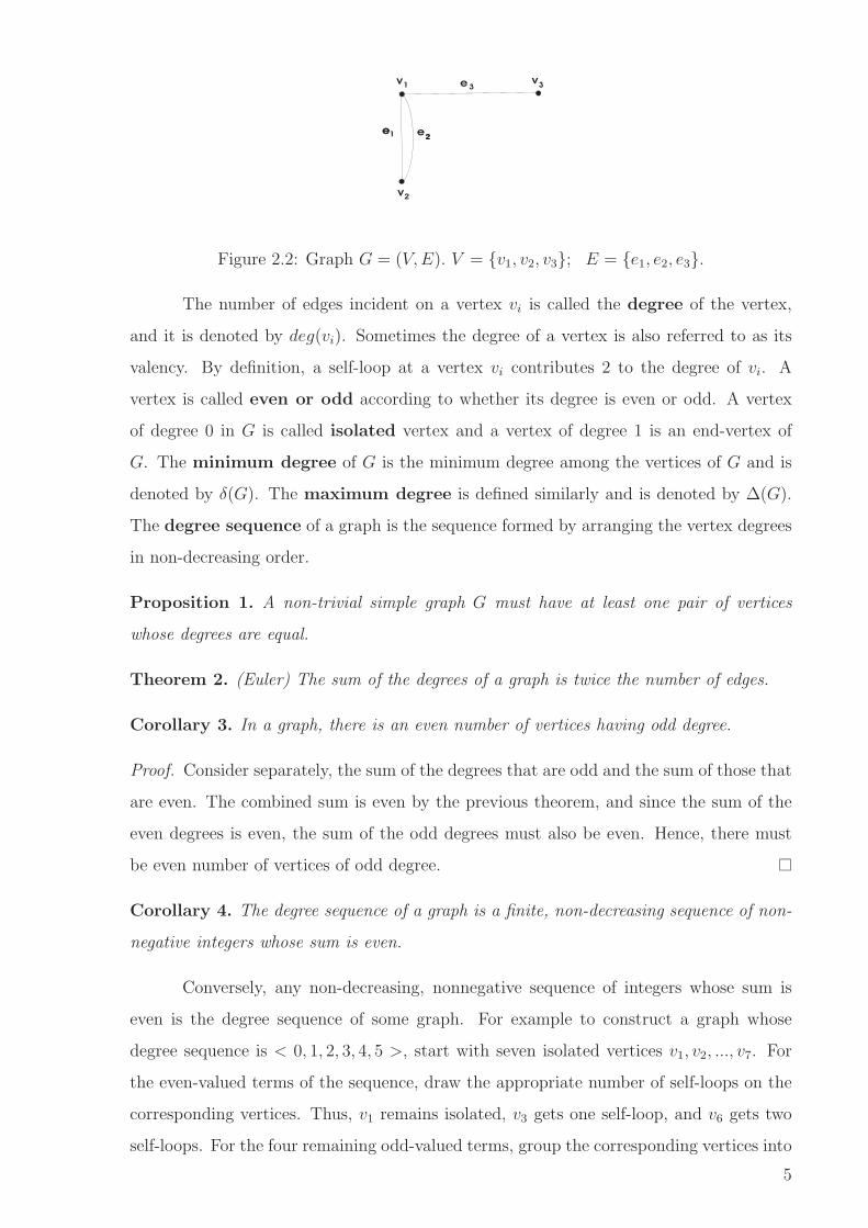
Conversely, any non-decreasing, nonnegative sequence of integers whose sum is
even is the degree sequence of some graph. For example to construct a graph whose
degree sequence is < 0, 1, 2, 3, 4, 5 >, start with seven isolated vertices v1, v2, ..., v7. For
the even-valued terms of the sequence, draw the appropriate number of self-loops on the
corresponding vertices. Thus, v1 remains isolated, v3 gets one self-loop, and v6 gets two
self-loops. For the four remaining odd-valued terms, group the corresponding vertices into
5
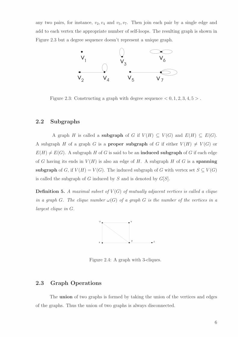
any two pairs, for instance, v2, v4 and v5, v7. Then join each pair by a single edge and
add to each vertex the appropriate number of self-loops. The resulting graph is shown in
Figure 2.3 but a degree sequence doesn’t represent a unique graph.
.v1
.v2 .v4
.v3
.v6
.v5 .v 7
Figure 2.3: Constructing a graph with degree sequence < 0, 1, 2, 3, 4, 5 > .
2.2 Subgraphs
A graph H is called a subgraph of G if V (H) ⊆ V (G) and E(H) ⊆ E(G).
A subgraph H of a graph G is a proper subgraph of G if either V (H) 6= V (G) or
E(H) 6= E(G). A subgraph H of G is said to be an induced subgraph of G if each edge
of G having its ends in V (H) is also an edge of H. A subgraph H of G is a spanning
subgraph of G, if V (H) = V (G). The induced subgraph of G with vertex set S ⊆ V (G)
is called the subgraph of G induced by S and is denoted by G[S].
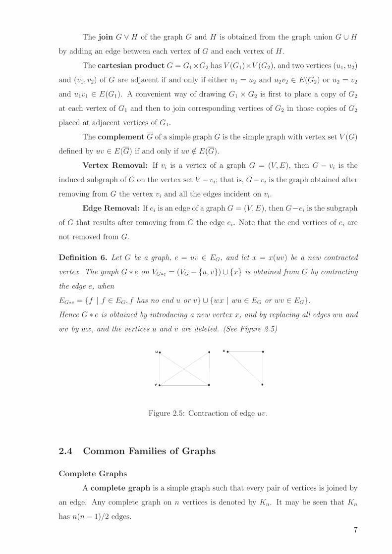
Definition 5. A maximal subset of V (G) of mutually adjacent vertices is called a clique
in a graph G. The clique number ω(G) of a graph G is the number of the vertices in a
largest clique in G.
.u
.x.y .z
.v
Figure 2.4: A graph with 3-cliques.
2.3 Graph Operations
The union of two graphs is formed by taking the union of the vertices and edges
of the graphs. Thus the union of two graphs is always disconnected.
6
The join G ∨ H of the graph G and H is obtained from the graph union G ∪ H
by adding an edge between each vertex of G and each vertex of H.
The cartesian product G = G1×G2 has V (G1)×V (G2), and two vertices (u1, u2)
and (v1, v2) of G are adjacent if and only if either u1 = u2 and u2v2 ∈ E(G2) or u2 = v2
and u1v1 ∈ E(G1). A convenient way of drawing G1 × G2 is first to place a copy of G2
at each vertex of G1 and then to join corresponding vertices of G2 in those copies of G2
placed at adjacent vertices of G1.
The complement G of a simple graph G is the simple graph with vertex set V (G)
defined by uv ∈ E(G) if and only if uv /∈ E(G).
Vertex Removal: If vi is a vertex of a graph G = (V,E), then G − vi is the
induced subgraph of G on the vertex set V −vi; that is, G−vi is the graph obtained after
removing from G the vertex vi and all the edges incident on vi.
Edge Removal: If ei is an edge of a graph G = (V,E), then G−ei is the subgraph
of G that results after removing from G the edge ei. Note that the end vertices of ei are
not removed from G.
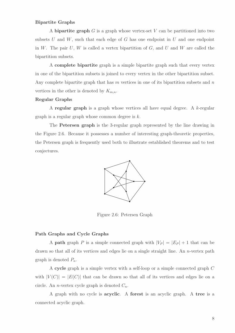
Definition 6. Let G be a graph, e = uv ∈ EG, and let x = x(uv) be a new contracted
vertex. The graph G ∗ e on VG∗e = (VG − {u, v}) ∪ {x} is obtained from G by contracting
the edge e, when
EG∗e = {f | f ∈ EG, f has no end u or v} ∪ {wx | wu ∈ EG or wv ∈ EG}.
Hence G ∗ e is obtained by introducing a new vertex x, and by replacing all edges wu and
wv by wx, and the vertices u and v are deleted. (See Figure 2.5)
Uu
Vv
Xx
Figure 2.5: Contraction of edge uv.
2.4 Common Families of Graphs
Complete Graphs
A complete graph is a simple graph such that every pair of vertices is joined by
an edge. Any complete graph on n vertices is denoted by Kn. It may be seen that Kn
has n(n − 1)/2 edges.
7
Bipartite Graphs
A bipartite graph G is a graph whose vertex-set V can be partitioned into two
subsets U and W , such that each edge of G has one endpoint in U and one endpoint
in W . The pair U , W is called a vertex bipartition of G, and U and W are called the
bipartition subsets.
A complete bipartite graph is a simple bipartite graph such that every vertex
in one of the bipartition subsets is joined to every vertex in the other bipartition subset.
Any complete bipartite graph that has m vertices in one of its bipartition subsets and n
vertices in the other is denoted by Km,n.
Regular Graphs
A regular graph is a graph whose vertices all have equal degree. A k-regular
graph is a regular graph whose common degree is k.
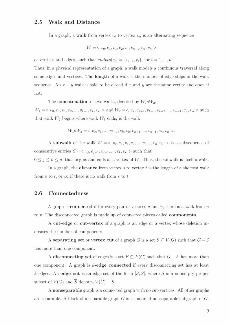
The Petersen graph is the 3-regular graph represented by the line drawing in
the Figure 2.6. Because it possesses a number of interesting graph-theoretic properties,
the Petersen graph is frequently used both to illustrate established theorems and to test
conjectures.
Figure 2.6: Petersen Graph
Path Graphs and Cycle Graphs
A path graph P is a simple connected graph with |VP | = |EP | + 1 that can be
drawn so that all of its vertices and edges lie on a single straight line. An n-vertex path
graph is denoted Pn.
A cycle graph is a simple vertex with a self-loop or a simple connected graph C
with |V (C)| = |E(C)| that can be drawn so that all of its vertices and edges lie on a
circle. An n-vertex cycle graph is denoted Cn.
A graph with no cycle is acyclic. A forest is an acyclic graph. A tree is a
connected acyclic graph.
8
2.5 Walk and Distance
In a graph, a walk from vertex v0 to vertex vn is an alternating sequence
W =< v0, e1, v1, e2, ..., vn−1, en, vn >
of vertices and edges, such that endpts(ei) = {vi−1, vi}, for i = 1, ..., n.
Thus, in a physical representation of a graph, a walk models a continuous traversal along
some edges and vertices. The length of a walk is the number of edge-steps in the walk
sequence. An x − y walk is said to be closed if x and y are the same vertex and open if
not.
The concatenation of two walks, denoted by W1oW2,
W1 =< v0, e1, v1, e2, ..., vk−1, ek, vk > and W2 =< vk, ek+1, vk+1, ek+2, ..., vn−1, en, vn > such
that walk W2 begins where walk W1 ends, is the walk
W1oW2 =< v0, e1, ..., vk−1, ek, vk, ek+1, ..., vn−1, en, vn >.
A subwalk of the walk W =< v0, e1, v1, e2, ..., vn−1, en, vn > is a subsequence of
consecutive entries S =< vj, ej+1, vj+1, ..., ek, vk > such that
0 ≤ j ≤ k ≤ n, that begins and ends at a vertex of W . Thus, the subwalk is itself a walk.
In a graph, the distance from vertex s to vertex t is the length of a shortest walk
from s to t, or ∞ if there is no walk from s to t.
2.6 Connectedness
A graph is connected if for every pair of vertices u and v, there is a walk from u
to v. The disconnected graph is made up of connected pieces called components.
A cut-edge or cut-vertex of a graph is an edge or a vertex whose deletion in-
creases the number of components.
A separating set or vertex cut of a graph G is a set S ⊆ V (G) such that G−S
has more than one component.
A disconnecting set of edges is a set F ⊆ E(G) such that G− F has more than
one component. A graph is k-edge connected if every disconnecting set has at least
k edges. An edge cut is an edge set of the form [S, S], where S is a nonempty proper
subset of V (G) and S denotes V (G) − S.
A nonseparable graph is a connected graph with no cut-vertices. All other graphs
are separable. A block of a separable graph G is a maximal nonseparable subgraph of G.
9
CHAPTER 3
VERTEX COLORINGS
The first known mention of coloring problems was in 1852, when August De Mor-
gan, Professor of Mathematics at University College, London, wrote Sir William Rowan
Hamilton in Dublin about a problem posed to him by a former student, named Francis
Guthrie. Guthrie noticed that it was possible to color the countries of England using
four colors so that no two adjacent countries were assigned the same color. The question
raised thereby was whether four colors would be sufficient for all possible decompositions
of the plane into regions.
The Poincare duality construction transforms this question into the problem of
deciding whether it is possible to color the vertices of every planar graph with four colors
so that no two vertices assigned the same color. Wolfgang Haken and Kenneth Appel
provided an affirmative solution in 1976 (Appel and Haken 1976).
3.1 The Minimization Problem for Vertex Coloring
In the most common kind of graph coloring, colors are assigned to the vertices.
From a standard mathematical prospective, the subset comprising all the vertices of a
given color would be regarded a cell of a partition of the vertex-set. Drawing the graph
with colors on the vertices is simply an intuitive way to represent such a partition.
We begin with a practical application of graph coloring known as the storage
problem. Suppose the Department of Chemistry of a college wants to store its chemicals.
It is a quite probable that some chemicals cause violent reactions when brought together.
Such chemicals are incompatible chemicals. For safe storage, incompatible chemicals
should be kept in distinct rooms. The easiest way to accomplish this is, of course, to store
one chemical in each room. But this is certainly not the best way of doing it since we
will be using more rooms than are really needed (unless, of course, all the chemicals are
mutually incompatible!). So we ask: What is the minimum number of rooms required to
store all the chemicals so that in each room only compatible chemicals are stored?
We convert the above storage problem into a problem in graphs. Form a graph
G = G(V,E) by making V correspond bijectively to the set of available chemicals and
making u adjacent to v if and only if the chemicals corresponding to u and v are incom-
patible. Then, any set of compatible chemical corresponds to a set of independent vertices
of G. Thus a safe storing of chemicals corresponds to a partition of V into independent
subsets of G. The cardinality of such a minimum partition of V is then the required
number of rooms. This minimum cardinality is called the chromatic number of the graph
G.
The chromatic number, χ(G), of a graph G is the minimum number of independent
subsets that partition the vertex set of G. Any such minimum partition is called a
chromatic partition of V (G) (Balakrishnan and Ranganathan 2000).
The storage problem just described is actually a vertex coloring problem of G.
A vertex coloring of G is a map f : V (G) → C, where C is a set of distinct colors;
it is proper if adjacent vertices of G receive distinct colors of C; that is, if uv ∈ E(G)
then f(u) 6= f(v). Thus χ(G) is the minimum cardinality of C for which there exists
a proper vertex coloring of G by colors of C. Clearly, in any proper vertex coloring of
G, the vertices that receive the same color are independent. The vertices that receive a
particular color make up a color class. Thus, in any chromatic partition of V (G), the parts
of the partition constitute the color classes. This allows an equivalent way of defining the
chromatic number.
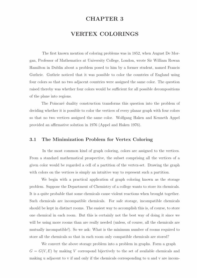
Definition 7. The chromatic number of a graph G is the minimum number of colors
needed for a proper vertex coloring of G. If χ(G) = k, G is said to be k-chromatic.
For example, the chromatic number of the graph in Figure 3.1 is 3.
1
2
1
2
1
2
3 1 1
3
3
2
Figure 3.1: A 3-chromatic graph
Definition 8. A k-coloring of a graph G is a vertex coloring of G that uses k colors.
Definition 9. A graph G is said to be k-colorable, if G admits a proper vertex coloring
using k colors.
Thus, χ(G) = k if graph G is k-colorable but not (k − 1)-colorable.
In considering the chromatic number of a graph only the adjacency of vertices is
taken into account. A graph with a self-loop is regarded as uncolorable, since the endpoint
11
of the self-loop is adjacent to itself. Moreover, a multiple adjacency has no more effect
on the colors of its endpoints than a single adjacency. As a consequence, we may restrict
ourselves to simple graphs when dealing with chromatic numbers.
It is clear that χ(G) = 1 if and only if G has no edges and χ(G) = 2 if and only if
G is bipartite.
3.2 Basic Principles for Calculating Chromatic Numbers
Although the chromatic number is one of the most studied parameters in graph
theory, no formula exists for the chromatic number of an arbitrary graph. Thus, for
the most part, one must be content with supplying bounds for the chromatic number of
graphs.
A few basic principles recur in many chromatic-number calculations. Now, we will
try to find upper and lower bound to provide a direct approach to the chromatic number
of a given graph.
Upper bound: Show χ(G) ≤ k by exhibiting a proper k-coloring of G.
Lower bound: Show χ(G) ≥ k by using properties of graph G, most especially, by
finding a subgraph that requires k-colors.
Proposition 10. Let G be a graph with k-mutually adjacent vertices. Then
χ(G) ≥ k.
Proof. Using fewer than k colors on graph G would result in a pair from the mutually
adjacent set of k vertices being assigned the same color.
Proposition 11. Let H be a subgraph of G. Then χ(G) ≥ χ(H).
Proof. Whatever colors are used on the vertices of subgraph H in a minimum coloring of
G can also be used in coloring of H by itself.
Corollary 12. Let G be a graph. Then χ(G) ≥ ω(G).
Proof. Since clique is a subgraph of G, we get this inequality.
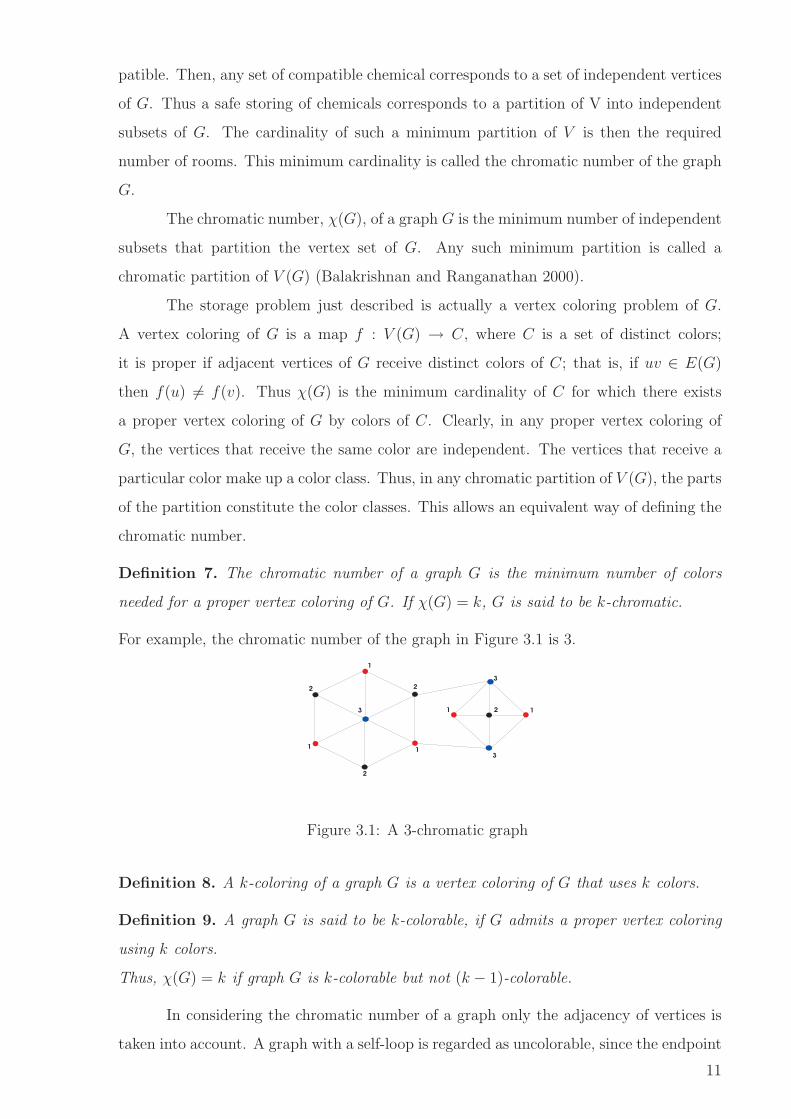
The 4-coloring of the graph G shown in Figure 3.2 establishes that χ(G) ≤ 4, and
the K4-subgraph (drawn in bold) shows that χ(G) ≥ 4. Hence, χ(G) = 4.
12
1
1
3
24
4
Figure 3.2: A 4-colorable graph
Proposition 13. Let G be any graph. Then
χ(G) ≥|V (G)|
α(G).
Proof. Given a k-coloring of G, the vertices being colored with the same color form an
independent set. Let G be a graph with n vertices and c a k-coloring of G. We define
Vi = {v | c(v) = i} for i = 0, 1, ..., k.
Each Vi is an independent set. Let α(G) be the independence number of G, we have
Vi ≤ α(G). Since
n = |V (G)| = |V1| + |V2| + ... + |Vk| ≤ k α(G) = χ(G) α(G)
we have
χ(G) ≥|V (G)|
α(G).
Most upper bounds on the chromatic number come from algorithms that produce
colorings. For example, assigning distinct colors to the vertices yields χ(G) ≤ n(G). This
bound is best possible, since χ(Kn) = n, but it holds with equality only for complete
graphs. We can improve a “best possible” bound by obtaining another bound that is
always at least as good. For example χ(G) ≤ n(G) uses nothing about the structure of
G; we can do better by coloring the vertices in some order and always using the “least
available” color.
Definition 14. The greedy coloring relative to a vertex ordering v1, v2, ..., vn of V (G) is
obtained by coloring vertices in order v1, v2, ..., vn, assigning to vi the smallest-indexed
color not already used on its lower-indexed neighbors.
13
Theorem 15. For any graph G,
χ(G) ≤ ∆(G) + 1.
Proof. In a vertex ordering, each vertex has at most ∆(G) earlier neighbors, so the greedy
coloring cannot be forced to use more than ∆(G) + 1 colors. This proves constructively
that χ(G) ≤ ∆(G) + 1.
The bound ∆(G)+1 is the worst upper bound that greedy coloring could produce.
Choosing the vertex ordering carefully yields improvements. We can avoid the trouble
caused by vertices of high degree by putting them at the beginning, where they won’t
have many earlier neighbors.
Proposition 16. If a graph G has the nonincreasing degree sequence d1 ≥ d2 ≥ ... ≥ dn,
then χ(G) ≤ 1 + maxi{min{di, i − 1}} (Welsh and Powel 1967).
Proof. We apply the greedy coloring to the vertices in nonincresing order of degree. When
we color the ith vertex vi, it has at most min{di, i − 1} earlier neighbors, so at most this
many colors appear on its earlier neighbors. Hence the color we assign to vi is at most
1 + min{di, i− 1}. This holds for each vertex, so we maximize over i to obtain the upper
bound on the maximum color used.
Theorem 17. For any graph G, χ(G) ≤ 1 + max(δ(G′)), where the maximum is taken
over all induced subgraphs G′ of G (Szekeres and Wilf 1968).
Proof. Let χ(G) = k, and let H be the minimal induced subgraph such that χ(H) = k.
So for any vertex v in H, the graph (H − v) is (k − 1)-colorable. Fix vertex v in H, and
consider any (k − 1) coloring of (H − v). In that case, if the degree of v in H is less than
(k − 1), it is possible to color the vertices of H using at most (k − 1) colors. Hence, the
degree of any vertex v in H is at least (k − 1). Thus, (k − 1) ≤ δ(H) ≤ max(δ(G′)).
3.3 Brooks’ Theorem
We are now prepared to present bounds for the chromatic number of a graph. We
give here several upper bounds, beginning with the best known and most applicable.
The bound χ(G) ≤ 1 + ∆(G) holds with equality for complete graphs and odd
cycles. By choosing the vertex ordering more carefully, we can show that these are es-
sentially the only such graphs. This implies, for example, that the Petersen graph is
3-colorable, without finding an explicit coloring. To avoid unimportant complications,
14
we phrase the statement only for connected graphs. It extends to all graphs because the
chromatic number of a graph is maximum chromatic number of its components. Many
proofs are known; we present a modification of the proof by (Melnikov and Vizing 1969).
For an alternative proof see (Lovasz 1975).
Theorem 18. (Brooks’ Theorem) If a connected graph G is neither an odd cycle nor a
complete graph, then χ(G) ≤ ∆(G).
Proof. If ∆(G) ≤ 2, then G is either a path or a cycle. For a path G (other than K1 and
K2), and for an even cycle G, χ(G) = 2 = ∆(G). According to our assumption G is not
an odd cycle. So let ∆(G) ≥ 3.
The proof is by contradiction. Suppose the result is not true. Then there exists a
minimal graph G of maximum degree ∆(G) ≥ 3 such that G is not ∆-colorable, but for
any vertex v of G, G − v is ∆(G − v)-colorable and therefore ∆-colorable.
Claim 1. Let v be any vertex of G. Then in any proper ∆-coloring of G − v, all the ∆-
colors must be used for coloring the neighbors of v in G. Otherwise, if some color i is not
represented in NG(v), then v could be colored using i, and this would give a ∆-coloring
of G, a contradiction to the choice of G. Thus, G is a regular graph satisfying claim 1.
For v ∈ V (G), let N(v) = v1, v2, ..., vn. In a proper ∆-coloring of G − v = H, let
vi receive color i, 1 ≤ i ≤ ∆. For i 6= j, let Hij be the subgraph of H induced by the
vertices receiving the ith and jth colors.
Claim 2. vi and vj belong to the same component of Hij. Otherwise, the colors i and
j can be interchanged in the component of Hij that contains the vertex vj. Such an
interchange of colors once again yields a proper ∆-coloring of H. In this new coloring,
both vi and vj receive the same color, namely, i, a contradiction to claim 1. This proves
claim 2.
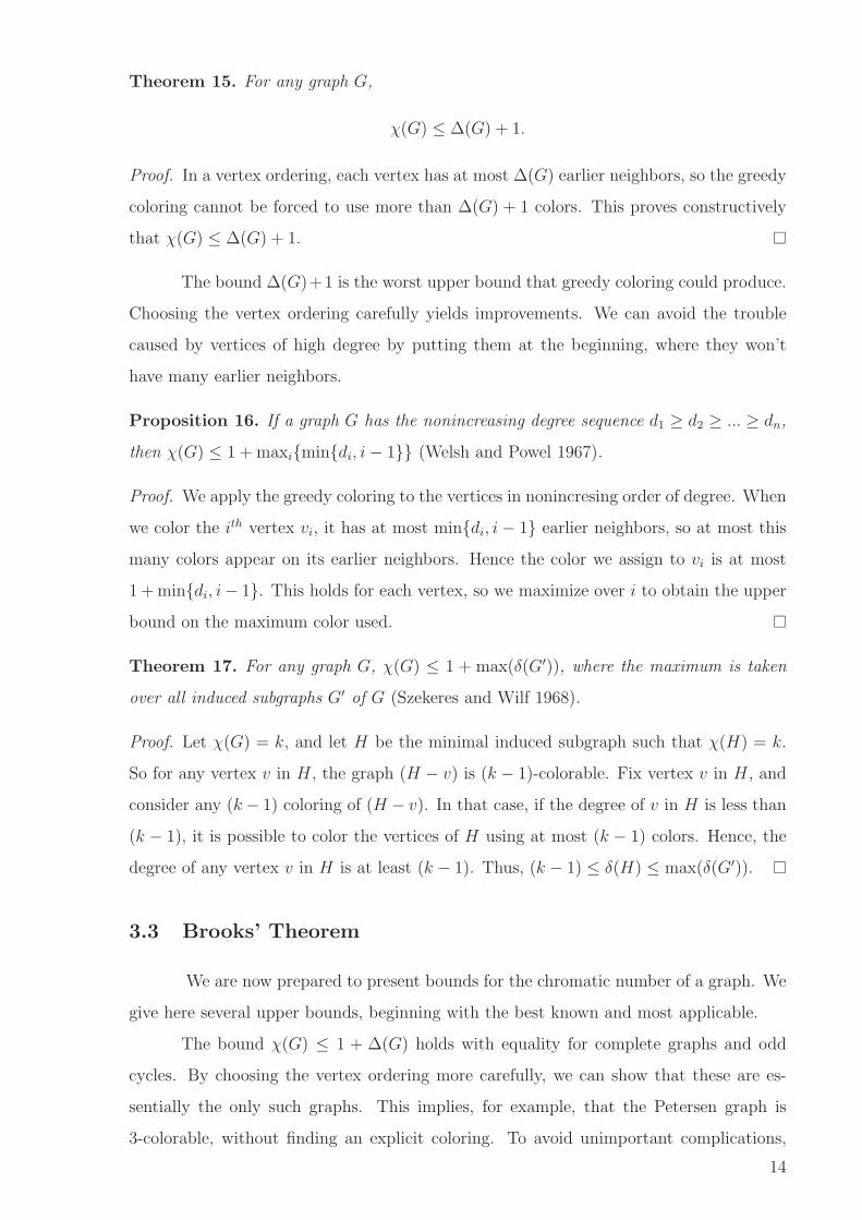
/v.i.(i).(j) .(i)
.(i)
.(j).(j)
.(j)
/v.j
/w /y
Figure 3.3: Brooks’ Theorem (a)
Claim 3. If Cij is the component of Hij containing vi and vj, then Cij is a path in Hij.
As before, NH(vi) contains exactly one vertex of color j. Further, Cij cannot contain a
vertex, say y, of degree at least 3; for, if y is the first such vertex on a vi − vj path in Cij
15
that has been colored, say, with i, then at least three neighbors of y in Cij have the color
j. Hence, we can recolor y in H with a color different from both i and j, and in this new
coloring of H, vi and vj would belong to distinct components of Hij. (See Figure 3.3.)
Note that by our choice of y, any vi − vj path in Hij must contain y. But this contradicts
claim 2.
/v.i
.(i)
.(k)
.(i)
.(j)
.(j)
.(j)
/v.j
/w
.(k).(k) /v
/kC.ij
C.ik
Figure 3.4: Brooks’ Theorem (b)
Claim 4. Cij ∩Cik = {vi} for j 6= k. Indeed, if w ∈ Cij ∩Cik, w 6= vi, then w is adjacent
to two vertices of color j on Cij and two vertices of color k on Cik. (See Figure 3.4.)
Again, we can recolor w in H by giving a color different from the colors of neighbors of
w in H. In this new coloring of H, vi and vj belong to distinct components of Hij, a
contradiction to claim 1. This completes the proof of claim 4.
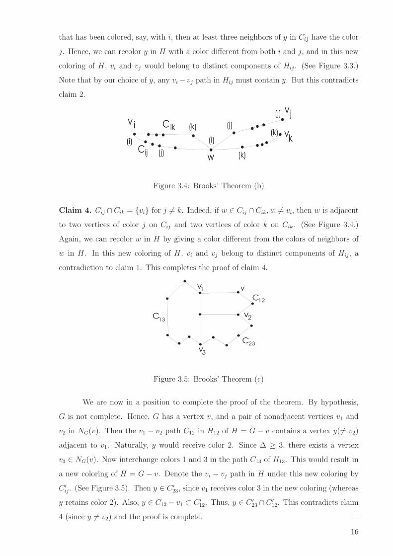
/v
/v
/v
C
C
1 /y
2
3
13
12
C23
Figure 3.5: Brooks’ Theorem (c)
We are now in a position to complete the proof of the theorem. By hypothesis,
G is not complete. Hence, G has a vertex v, and a pair of nonadjacent vertices v1 and
v2 in NG(v). Then the v1 − v2 path C12 in H12 of H = G − v contains a vertex y(6= v2)
adjacent to v1. Naturally, y would receive color 2. Since ∆ ≥ 3, there exists a vertex
v3 ∈ NG(v). Now interchange colors 1 and 3 in the path C13 of H13. This would result in
a new coloring of H = G − v. Denote the vi − vj path in H under this new coloring by
C ′
ij. (See Figure 3.5). Then y ∈ C ′
23, since v1 receives color 3 in the new coloring (whereas
y retains color 2). Also, y ∈ C12 − v1 ⊂ C ′
12. Thus, y ∈ C ′
23 ∩ C ′
12. This contradicts claim
4 (since y 6= v2) and the proof is complete.
16
3.4 Chromatic Numbers of Generated Graphs
Proposition 19. For the disjoint union,
χ(G ∪ H) = max{χ(G), χ(H)}.
Proposition 20. The join of the graphs G and H has chromatic number
χ(G ∨ H) = χ(G) + χ(H).
Proof. Lower Bound: In the join G∨H, no color used on the subgraph G can be the same
as a color used on the subgraph H, since every vertices of G is adjacent to every vertices
of H. Since χ(G) colors are required for the subgraph G and χ(H) colors are required for
the subgraph H, it follows that χ(G ∨ H) ≥ χ(G) + χ(H).
Upper Bound: Just use any χ(G) colors to properly color the subgraph G of G ∨ H and
use χ(H) different colors to color the subgraph H.
Proposition 21. (Vizing 1963, Albert 1964)
χ(G × H) = max{χ(G), χ(H)}.
Proof. The cartesian product χ(G × H) contains copies of G and H as subgraphs so
χ(G × H) ≥ max{χ(G), χ(H)}.
Let k = max{χ(G), χ(H)}. To prove the upper bound, we produce a proper k-coloring of
G × H using optimal colorings of G and H. Let g be a proper χ(G)- coloring of G, and
let h be a proper χ(H)- coloring of H. Define a coloring f of G×H by letting f(u, v) be
the congruence class of g(u) + h(v) modulo k. Thus f assigns color to V (G × H) from a
set of size k.
We claim that f properly colors G×H. If (u, v) and (u′, v′) are adjacent in G×H,
then g(u) + h(v) and g(u′) + h(v′) agree in one summand and differ by between 1 and k
in the other. Since the difference of the two sums is between 1 and k, they lie in different
congruence classes modulo k.
3.5 Chromatic Numbers for Common Graph Families
It is straightforward to establish the chromatic number of graphs in some of the
most common graph families, by using the basic principles given above.
17
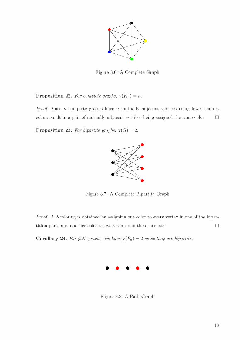
Figure 3.6: A Complete Graph
Proposition 22. For complete graphs, χ(Kn) = n.
Proof. Since n complete graphs have n mutually adjacent vertices using fewer than n
colors result in a pair of mutually adjacent vertices being assigned the same color.
Proposition 23. For bipartite graphs, χ(G) = 2.
Figure 3.7: A Complete Bipartite Graph
Proof. A 2-coloring is obtained by assigning one color to every vertex in one of the bipar-
tition parts and another color to every vertex in the other part.
Corollary 24. For path graphs, we have χ(Pn) = 2 since they are bipartite.
Figure 3.8: A Path Graph
18
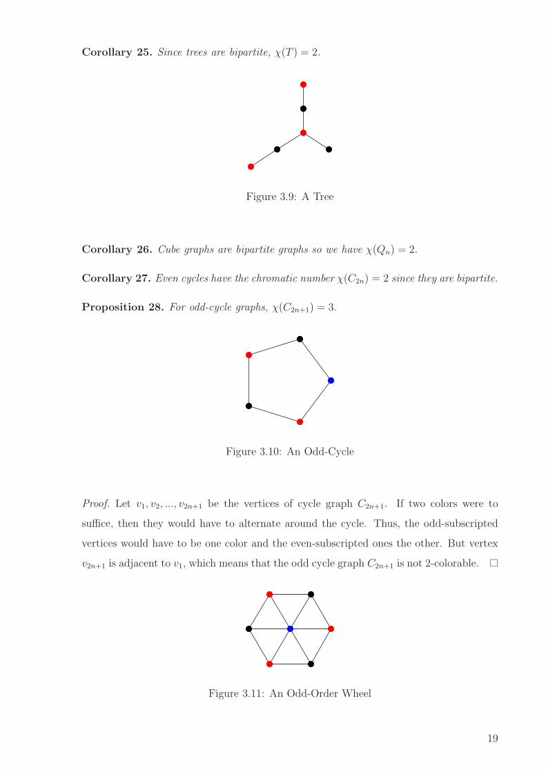
Corollary 25. Since trees are bipartite, χ(T ) = 2.
Figure 3.9: A Tree
Corollary 26. Cube graphs are bipartite graphs so we have χ(Qn) = 2.
Corollary 27. Even cycles have the chromatic number χ(C2n) = 2 since they are bipartite.
Proposition 28. For odd-cycle graphs, χ(C2n+1) = 3.
Figure 3.10: An Odd-Cycle
Proof. Let v1, v2, ..., v2n+1 be the vertices of cycle graph C2n+1. If two colors were to
suffice, then they would have to alternate around the cycle. Thus, the odd-subscripted
vertices would have to be one color and the even-subscripted ones the other. But vertex
v2n+1 is adjacent to v1, which means that the odd cycle graph C2n+1 is not 2-colorable.
Figure 3.11: An Odd-Order Wheel
19
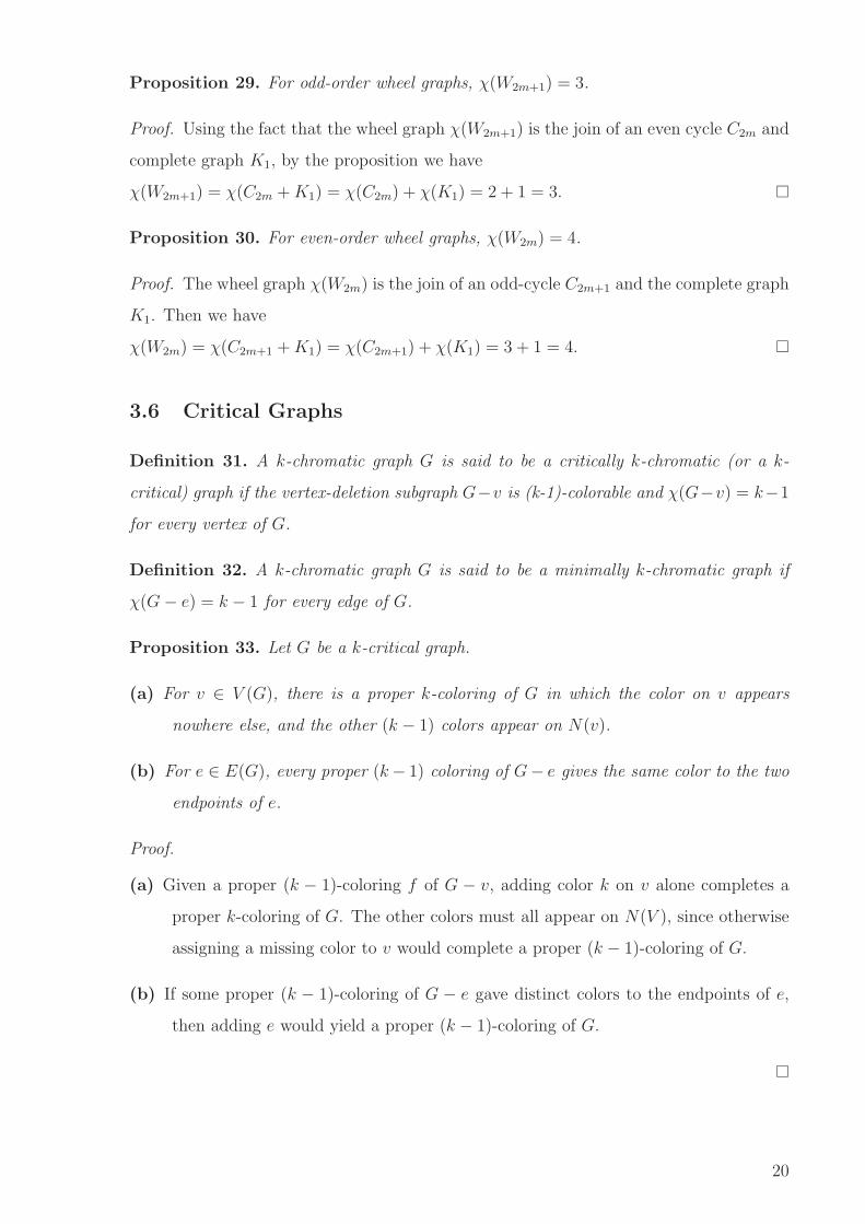
Proposition 29. For odd-order wheel graphs, χ(W2m+1) = 3.
Proof. Using the fact that the wheel graph χ(W2m+1) is the join of an even cycle C2m and
complete graph K1, by the proposition we have
χ(W2m+1) = χ(C2m + K1) = χ(C2m) + χ(K1) = 2 + 1 = 3.
Proposition 30. For even-order wheel graphs, χ(W2m) = 4.
Proof. The wheel graph χ(W2m) is the join of an odd-cycle C2m+1 and the complete graph
K1. Then we have
χ(W2m) = χ(C2m+1 + K1) = χ(C2m+1) + χ(K1) = 3 + 1 = 4.
3.6 Critical Graphs
Definition 31. A k-chromatic graph G is said to be a critically k-chromatic (or a k-
critical) graph if the vertex-deletion subgraph G−v is (k-1)-colorable and χ(G−v) = k−1
for every vertex of G.
Definition 32. A k-chromatic graph G is said to be a minimally k-chromatic graph if
χ(G − e) = k − 1 for every edge of G.
Proposition 33. Let G be a k-critical graph.
(a) For v ∈ V (G), there is a proper k-coloring of G in which the color on v appears
nowhere else, and the other (k − 1) colors appear on N(v).
(b) For e ∈ E(G), every proper (k − 1) coloring of G− e gives the same color to the two
endpoints of e.
Proof. .
(a) Given a proper (k − 1)-coloring f of G − v, adding color k on v alone completes a
proper k-coloring of G. The other colors must all appear on N(V ), since otherwise
assigning a missing color to v would complete a proper (k − 1)-coloring of G.
(b) If some proper (k − 1)-coloring of G − e gave distinct colors to the endpoints of e,
then adding e would yield a proper (k − 1)-coloring of G.
20
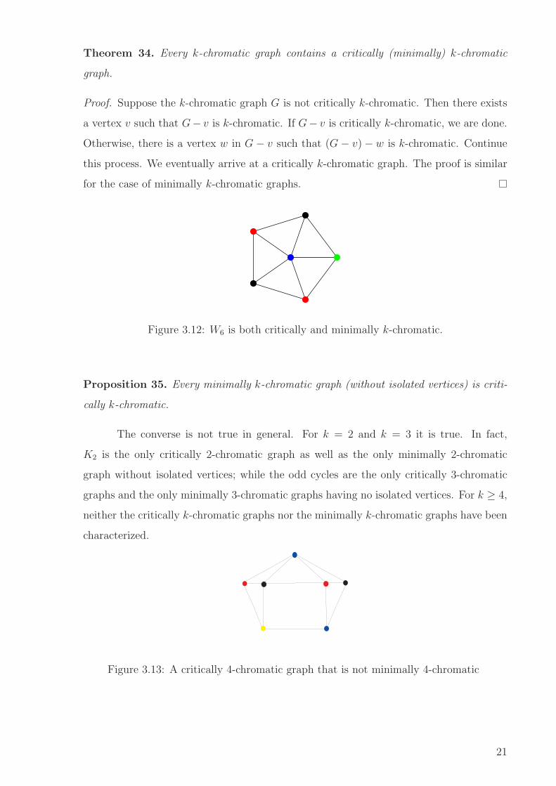
Theorem 34. Every k-chromatic graph contains a critically (minimally) k-chromatic
graph.
Proof. Suppose the k-chromatic graph G is not critically k-chromatic. Then there exists
a vertex v such that G− v is k-chromatic. If G− v is critically k-chromatic, we are done.
Otherwise, there is a vertex w in G − v such that (G − v) − w is k-chromatic. Continue
this process. We eventually arrive at a critically k-chromatic graph. The proof is similar
for the case of minimally k-chromatic graphs.
Figure 3.12: W6 is both critically and minimally k-chromatic.
Proposition 35. Every minimally k-chromatic graph (without isolated vertices) is criti-
cally k-chromatic.
The converse is not true in general. For k = 2 and k = 3 it is true. In fact,
K2 is the only critically 2-chromatic graph as well as the only minimally 2-chromatic
graph without isolated vertices; while the odd cycles are the only critically 3-chromatic
graphs and the only minimally 3-chromatic graphs having no isolated vertices. For k ≥ 4,
neither the critically k-chromatic graphs nor the minimally k-chromatic graphs have been
characterized.
Figure 3.13: A critically 4-chromatic graph that is not minimally 4-chromatic
21
A k-chromatic subgraph of G of minimum order is critically k-chromatic, while a
k-chromatic subgraph of G of minimum size is minimally k-chromatic. Every critically
k-chromatic graph is nonseperable and every minimally k-chromatic graph without
isolated vertices is nonseperable.
Theorem 36. If G is a critically k-chromatic graph then G is (k − 1)-edge connected.
(Equivalently, any connected minimally k-chromatic graph is (k − 1)-edge connected.)
Proof. If k = 2, the graph is K2, which is 1-edge-connected. If k = 3, the graph is an odd
cycle, which is 2-edge connected. Let k ≥ 4. Suppose G is not (k − 1)-edge connected.
Then there is a partition of the vertex set of G into two sets X and Y such that the
cardinality of cut [X,Y ] is less than (k − 1). So the subgraphs induced by X and Y are
(k − 1)-colorable. Since the chromatic number of G is k, cut [X,Y ] should have at least
(k − 1) edges. This contradiction establishes that G is (k − 1)-edge connected.
Theorem 37. If G is critically k-chromatic (or connected and minimally k-chromatic),
then no vertex of G has degree less than k − 1, i.e. δ(G) ≥ k − 1.
Proof. Suppose that v were a vertex of degree less than k − 1. Since G is k-critical, the
vertex deletion subgraph G− v is (k − 1)-colorable. The colors assigned to the neighbors
of v would not include all the colors of (k − 1)-coloring because vertex v has fewer than
(k − 1) neighbors. Thus, if v were restored to the graph, it could be colored with any
one of the k − 1 colors that was not used on any of its neighbors. This would achieve a
(k − 1)-coloring of G, which is a contradiction. Thus δ(G) ≥ k − 1.
Corollary 38. Every k-chromatic graph has at least k vertices of degree at least k − 1.
Proof. Let G be a k-chromatic graph and let H be a k-critical subgraph of G. By the
Theorem 37, each vertex of H has degree at least k − 1 in H, and hence also in G. Since
H is k-chromatic, clearly has at least k vertices.
Proposition 39. A critically k-chromatic graph G with exactly one vertex whose degree
exceeds (k − 1) is minimally k-chromatic.
Proof. Since G is critically k-chromatic, the degree of each vertex is at least (k − 1). In
this case, the degree of each vertex is (k − 1) except for one vertex. If e is any edge of G,
δ(G− e) = k − 2. Then χ(G− e) ≤ 1 + max δ(G′), where G′ is any induced subgraph of
(G − e). Thus χ(G − e) ≤ 1 + (k − 2) = k − 1. Since the minimum degree in (G − e) is
k − 2, χ(G − e) = k − 1.
22
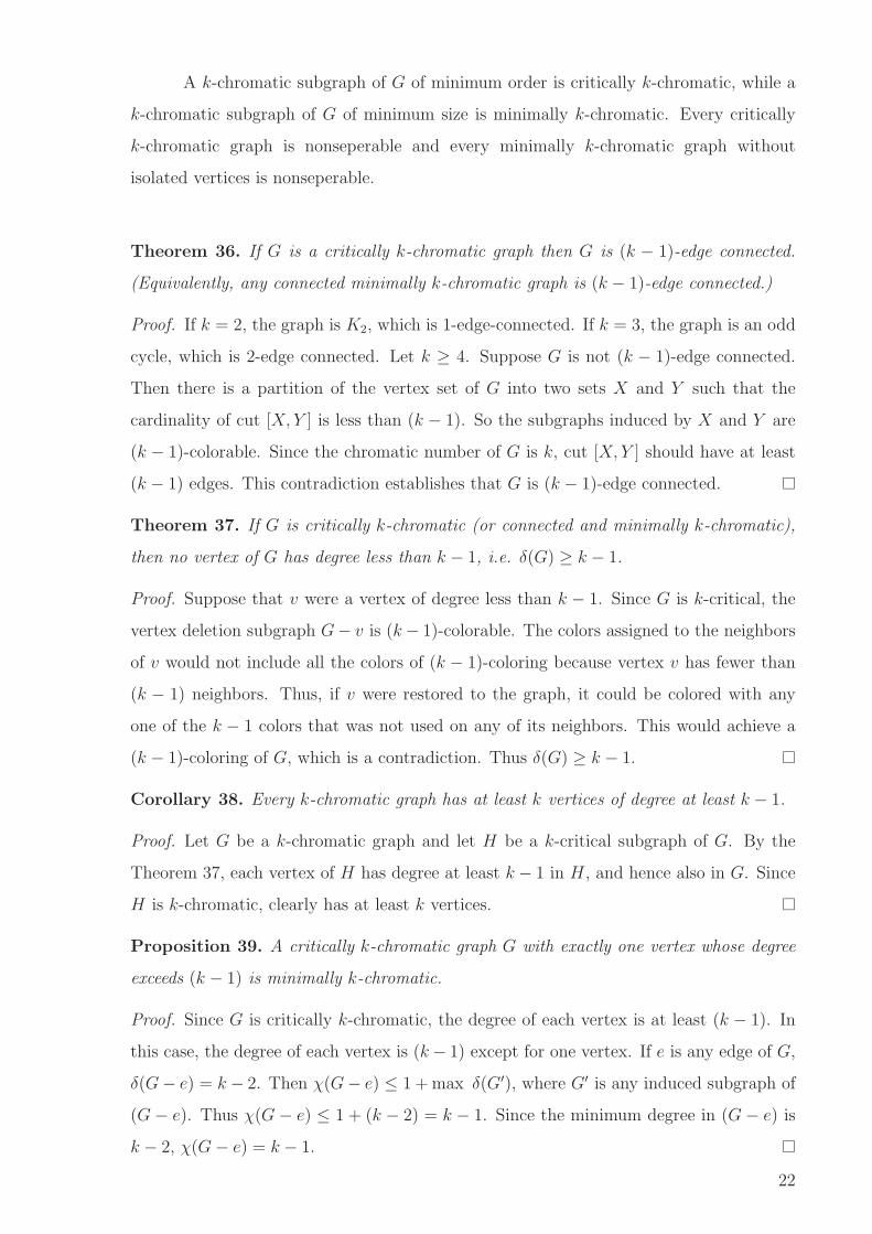
3.7 Obstructions to k-Chromaticity
Definition 40. An obstruction to k-chromaticity (or k-obstruction) is a subgraph that
forces every graph that contains it to have chromatic number greater than k.
The complete graph Kk+1 is an obstruction to k-chromaticity.
Remark 41. If any edge is deleted from a (k + 1)-critical graph, then by the definition,
the resulting graph is not an obstruction to k-chromaticity. Thus, a (k + 1)-critical graph
is an edge-minimal obstruction to k-chromaticity.
Definition 42. A set {Gj} of chromatically (k + 1)-critical graphs is a complete set of
obstructions if every (k + 1)-chromatic graph contains at least one member of {Gj} as a
subgraph.
The singleton set {K2} is a complete set of obstructions to 1-chromaticity.
The set {C2j+1 | j = 0, 1, ...} of odd cycles is a complete set of 2-obstructions since a graph
is bipartite if and only if it contains no odd cycles. Although the even order wheel graphs
W2m with m ≥ 2 are 4-critical, they do not form a complete set of 3-obstructions, since
there are 4-chromatic graphs that contain no such wheel. The graph in Figure 3.14 does
not contain an even-order wheel graph, but case-by-case analysis can be used to show
that the graph is 4-chromatic.
Figure 3.14: A 4-chromatic graph that contains no W2m
Remark 43. A more elegant approach to proving that the graph of Figure 3.14 requires
at least four colors is based on consideration of the maximum number of vertices that can
be colored with a single color.
3.8 Chromatic Polynomials
In the study of colorings, some insight can be gained by considering not only the
existence of colorings but also the number of such colorings. This approach was developed
23
by (Birkhoff 1912) as a possible means of attacking the four-color conjecture. We shall
denote the number of distinct k-colorings of G by πk(G); thus πk(G) > 0 if and only if
G is k-colorable. Two colorings are to be regarded as distinct if some vertex is assigned
different colors in the two colorings; in other words, if (V1, V2, ..., Vk) and (V ′
1 , V′
2 , ..., V′
k)
are two colorings, then (V1, V2, ..., Vk) = (V ′
1 , V′
2 , ..., V′
k) if and only if Vi = V ′
i for 1 ≤ i ≤ k.
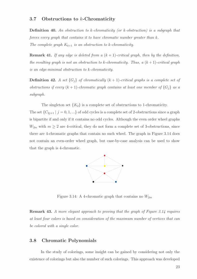
For example, a triangle has the six distinct 3-colorings shown in Figure 3.15. Note that
even though there is exactly one vertex of each color in each coloring, we still regard these
six colorings as distinct. When coloring the vertices of Kn, complement of the complete
Figure 3.15: Six distinct 3-colorings of K3
graph with n vertices, we can use any of the k-colors at each vertex no matter what colors
we have used at other vertices. Therefore
πk(Kn) = kn. On the other hand, when we color the vertices of Kn, there are k choices
of color for the first vertex, (k − 1) choices for the second, (k − 2) for the third, and so
on. Thus, in this case,
πk(Kn) = k(k − 1)...(k − n + 1).
Theorem 44. If G is a simple graph and e ∈ E(G), then
πk(G) = πk(G − e) − πk(G ∗ e).
Proof. Let u and v be the ends of e. To each k-coloring of G − e that assigns the same
color to u and v, there corresponds a k-coloring of G∗e in which the vertex of G∗e formed
by identifying u and v is assigned the common color of u and v. This correspondence is
clearly a bijection. Therefore πk(G ∗ e) is precisely the number of k-colorings of G − e in
which u and v are assigned the same color.
Also, since each k-coloring of G− e that assigns different colors to u and v is a k-coloring
of G, and conversely, πk(G) is the number of k-colorings G − e in which u and v are
assigned different colors. It follows that,
πk(G − e) = πk(G) + πk(G ∗ e).
24
Theorem 45. For a simple graph G of order n and size m, πk(G) is a monic polynomial of
degree n in k with integer coefficients and constant term zero. In addition, its coefficients
alternate in sign and the coefficient of kn−1 is −m.
Proof. Proof is induction on m. If m = 0, G is Kn and πk(Kn) = kn, and the statement
of the theorem is trivially true in this case. Suppose, now, that the theorem holds for all
graphs with fewer than m edges, where m ≥ 1. Let G be any simple graph of order n
and size m, and let e be any edge of G. Both G − e and G ∗ e (after removal of multiple
edges, if necessary) are simple graphs with at most (m−1) edges, and hence, by induction
hypothesis,
πk(G − e) = kn − a0kn−1 + a1k
n−2 + ... + (−1)n−1an−2k,
and
πk(G ∗ e) = kn−1 − b1kn−2 + ... + (−1)n−2bn−2k,
where a0, ..., an−1; b1, ..., bn−2 are nonnegative integers (so that the coefficients alternate
in sign), and a0 is the number of edges in G − e, which is m − 1. By Theorem 44,
πk(G) = πk(G − e) − πk(G ∗ e), and hence
πk(G) = kn − (a0 + 1)kn−1 + (a1 + b1)kn−2 − ... + (−1)n−1(an−2 + bn−2)k.
Since a0 + 1 = m, πk(G) has all the stated properties.
Proposition 46. A simple graph G on n vertices is a tree if and only if
πk(T ) = k(k − 1)n−1.
Proof. Let G be a tree. We prove that πk(T ) = k(k − 1)n−1 by induction on n. If
n = 1, the result is trivial. So assume the result for trees with at most (n − 1) vertices,
n ≥ 2. Let G be a tree with n vertices, and e be a pendant edge of G. By Theorem 44,
πk(G) = πk(G− e)−πk(G ∗ e). Now, G− e is a forest with two component trees of orders
(n−1) and 1, and hence πk(G−e) = (k(k−1)n−2)k. Since G∗e is a tree with (n−1) vertices,
πk(G ∗ e) = k(k − 1)n−2. Thus, πk(G ∗ e) = (k(k − 1)n−2)k − k(k − 1)n−2 = k(k − 1)n−1.
Conversely, assume that G is a simple graph with
πk(G) = k(k− 1)n−1 = kn − (n− 1)kn−1 + ...+(−1)n−1k. Hence, by Theorem 45, G has n
vertices and (n− 1) edges. Further, the last term, (−1)n−1k, ensures that G is connected.
Hence G is a tree.
Since the number of proper k-colorings is unaffected by multiple edges, we discard
multiple copies of edges that arise from the contraction, keeping only one copy of each to
form a simple graph.
25
By virtue of corollary, we can now refer to the function πk(G) as the chromatic
polynomial of G. Theorem 44 provides a means of calculating the chromatic polynomial
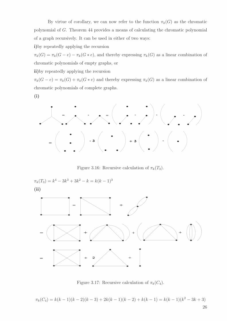
of a graph recursively. It can be used in either of two ways:
i)by repeatedly applying the recursion
πk(G) = πk(G − e) − πk(G ∗ e), and thereby expressing πk(G) as a linear combination of
chromatic polynomials of empty graphs, or
ii)by repeatedly applying the recursion
πk(G − e) = πk(G) + πk(G ∗ e) and thereby expressing πk(G) as a linear combination of
chromatic polynomials of complete graphs.
(i)
= - = - --
=- 3 + 3 -
Figure 3.16: Recursive calculation of πk(T3).
πk(T3) = k4 − 3k3 + 3k2 − k = k(k − 1)3
(ii)
= +
= + + +
= + 2 +
Figure 3.17: Recursive calculation of πk(C4).
πk(C4) = k(k − 1)(k − 2)(k − 3) + 2k(k − 1)(k − 2) + k(k − 1) = k(k − 1)(k2 − 3k + 3)
26
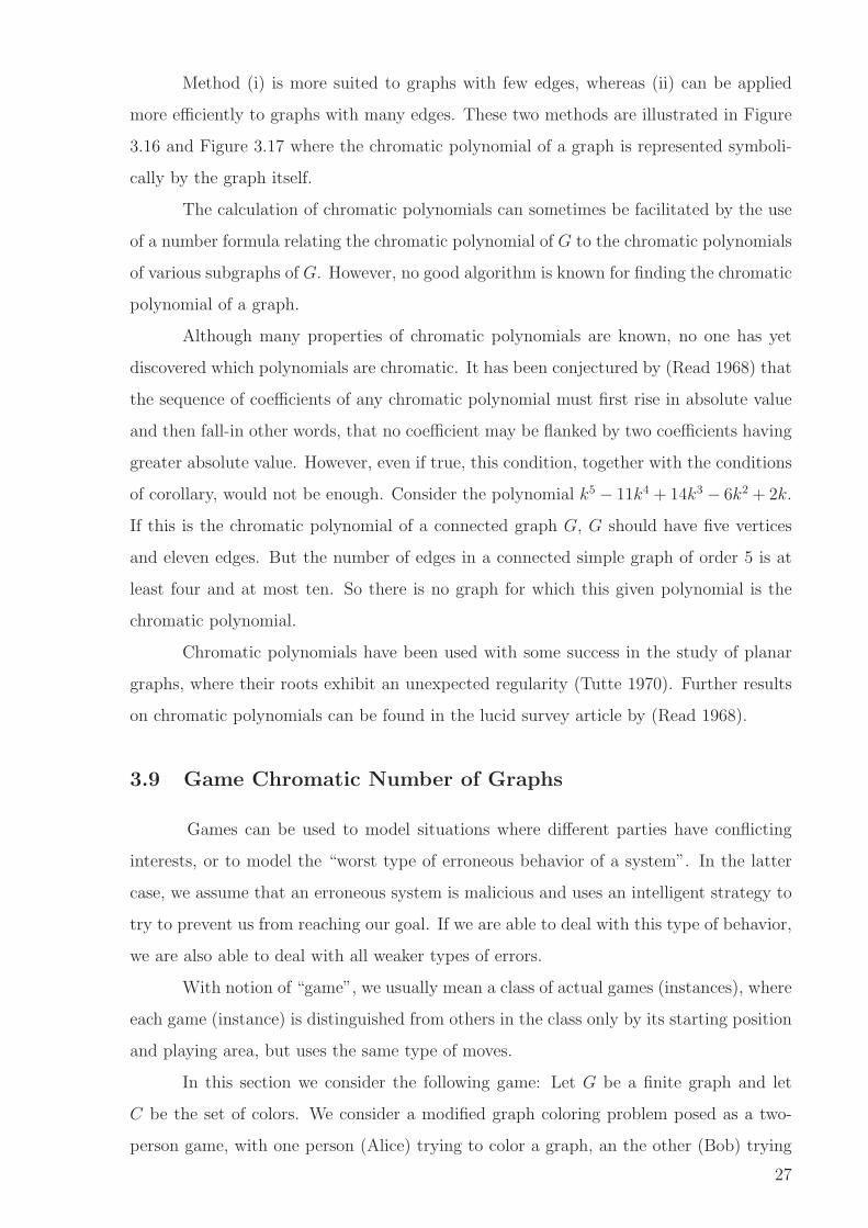
Method (i) is more suited to graphs with few edges, whereas (ii) can be applied
more efficiently to graphs with many edges. These two methods are illustrated in Figure
3.16 and Figure 3.17 where the chromatic polynomial of a graph is represented symboli-
cally by the graph itself.
The calculation of chromatic polynomials can sometimes be facilitated by the use
of a number formula relating the chromatic polynomial of G to the chromatic polynomials
of various subgraphs of G. However, no good algorithm is known for finding the chromatic
polynomial of a graph.
Although many properties of chromatic polynomials are known, no one has yet
discovered which polynomials are chromatic. It has been conjectured by (Read 1968) that
the sequence of coefficients of any chromatic polynomial must first rise in absolute value
and then fall-in other words, that no coefficient may be flanked by two coefficients having
greater absolute value. However, even if true, this condition, together with the conditions
of corollary, would not be enough. Consider the polynomial k5 − 11k4 + 14k3 − 6k2 + 2k.
If this is the chromatic polynomial of a connected graph G, G should have five vertices
and eleven edges. But the number of edges in a connected simple graph of order 5 is at
least four and at most ten. So there is no graph for which this given polynomial is the
chromatic polynomial.
Chromatic polynomials have been used with some success in the study of planar
graphs, where their roots exhibit an unexpected regularity (Tutte 1970). Further results
on chromatic polynomials can be found in the lucid survey article by (Read 1968).
3.9 Game Chromatic Number of Graphs
Games can be used to model situations where different parties have conflicting
interests, or to model the “worst type of erroneous behavior of a system”. In the latter
case, we assume that an erroneous system is malicious and uses an intelligent strategy to
try to prevent us from reaching our goal. If we are able to deal with this type of behavior,
we are also able to deal with all weaker types of errors.
With notion of “game”, we usually mean a class of actual games (instances), where
each game (instance) is distinguished from others in the class only by its starting position
and playing area, but uses the same type of moves.
In this section we consider the following game: Let G be a finite graph and let
C be the set of colors. We consider a modified graph coloring problem posed as a two-
person game, with one person (Alice) trying to color a graph, an the other (Bob) trying
27
to prevent this from happening. Alice and Bob alternate turns, with Alice having the
first move. A move consist of selecting a previously uncolored vertex x and assigning
to it a color from the color set C distinct from the colors assigned previously (by either
player) to neighbors of x. If after n = |V (G)| moves, the graph G is colored, Alice is the
winner. Bob wins if an impass is reached before all nodes in the graph are colored, i.e.,
for every uncolored vertex x and every color α from C, x is adjacent to a vertex having
color α. The game chromatic number of a graph G = (V,E), denoted by χg(G), is the
least cardinality of a color set C for which Alice has a winning strategy. This parameter
is well-defined, since Alice always wins if |C| = |V |.
The notion of a graph coloring game was first introduced by (Bodlaender 1991).
It seems to be very difficult to determine or estimate the game chromatic number of even
small graphs. However, for special classes of graphs, non-trivial upper and lower bounds
for the game chromatic numbers are obtained. The easiest case is the class of forests. It
was proved by Faigle, Kern, Kierstead, and Trotter that the game chromatic number of
a forest is at most 4, and that there are forests of game chromatic number 4 (Faigle et
al. 1993). The game chromatic number of outerplanar graphs was studied by (Zue 1999,
Kierstead 1994). It was shown in (Kierstead 1994) that outerplanar graphs have game
chromatic number at most 8, and this upper bound is reduced to 7 (Zue 1999). On the
other hand, there are outerplanar graphs with game chromatic number 6. It is unknown
if there are outerplanar graphs with game chromatic number 7.
28
CHAPTER 4
VERTEX COLORING WITH webMATHEMATICA
4.1 Mathematica and Combinatorica Package
Mathematica, created by Stephen Wolfram, is a software system in which you
can investigate mathematics, perform calculations, create graphics, and write programs.
Mathematica commands are typed on a graphical user interface containing menu options.
Combinatorica, an extension to the popular computer algebra system Mathemat-
ica, is the most comprehensive software available for educational and research applications
of discrete mathematics, particularly combinatorics and graph theory. It has been per-
haps the most widely used software for teaching and research in discrete mathematics
since its initial release in (Skiena 1990).
The goal of Combinatorica is to advance the study of combinatorics and graph
theory by making a wide variety of functions available for active experimentation. We
developed this package and called ColorG. We consider many classes of graphs, how to
color and construct them by using our package ColorG.
4.2 The Concept of webMathematica
The growing popularity of the internet and the increasing number of computers
connected to it, make it an ideal framework for remote education. Many disciplines are
rethinking their traditional philosophies and techniques to adapt to the new technologies.
Web-based education is an effective framework for such learning, which simplifies theory
understanding, encourages learning by discovery and experimentation and undoubtedly
makes the learning process more pleasant. There is a need for adequate tools to help in the
elaboration of courses that might make it possible to express all the possibilities offered
by online teaching. webMathematica is a web-based technology developed by Wolfram
Research that allows the generation of dynamic web content with Mathematica. With
this technology, distance education students should be able to explore and experiment
with mathematical concepts.
webMathematica is a web version of Mathematica that delivers interactive calcu-
lations and visualizations over the web. It allows a web site to return results that are
marked up with Mathematica computations. When a request is made for one of these
pages, the Mathematica commands are evaluated and any computed results inserted into
the page. This is done with the standard Java templating mechanism, JavaServer Pages.
webMathematica technology uses the request/response standard followed by web
servers. Input can come from HTML forms, applets, javascript, and web-enabled appli-
cations. It is also possible to send data files to a webMathematica server for processing.
Output can use many different formats, such as HTML, images, Mathematica notebooks,
MathML, SVG, PostScript and PDF.
4.3 Coloring Common Graph Families
Finding a minimum coloring can be done using brute-force search but to effectively
color large graphs heuristics and usually quite effective. ColorG considers a heuristic
approach to graph coloring. We use some commands in the ColorG package to color the
graphs and to give web-based examples with webMathematica.
We use mainly the following ColorVertices module.
ColorVertices[g−] := Module[{c, p, s},
c = VertexColoring[g];
p = Table[Flatten[Position[c, i]], {i, 1, Max[c]}];
s = ShowLabeledGraph[ Highlight[g, p]]]
The module ColorVertices colors vertices of the given graph g properly.
webMathematica allows the generation of dynamic web content with Mathematica. The
following example draws the given graph and colors the vertices.
<FORM ACTION="vertex.jsp" METHOD="POST">
<p>Please select one of the following graphs and
input into the box:(1,2,3,or 4) </p>
<p>1-CompleteGraph,</p> <p>2-RandomTree, </p>
<p>3-Wheel,</p> <p>4-Cycle)</p>
<msp:allocateKernel>
<INPUT type="text" name="m" ALIGN="LEFT" size="6"
value="<msp:evaluate> MSPValue[$$m,"1"]</msp:evaluate>" />
Input the number of the vertices for the selected graph:
30
<INPUT type="text" name="n" ALIGN="LEFT" size="6"
value="<msp:evaluate> MSPValue[$$n,"5"]</msp:evaluate>" />
<msp:evaluate> <<DiscreteMath`ColorG`
</msp:evaluate>
<h3>Vertex coloring of the graph is </h3>
<msp:evaluate> MSPBlock[{$$m,$$n},
Which[$$m==1,MSPShow[ColorVertices[CompleteGraph[$$n]]],
$$m==2, MSPShow[ColorVertices[RandomTree[$$n]]],
$$m==3, MSPShow[ColorVertices[Wheel[$$n]]],
$$m==4, MSPShow[ColorVertices[Cycle[$$n]]]]]
</msp:evaluate>
The Chromatic Number of the selected graph is <msp:evaluate>
MSPBlock[{$$m,$$n},
Which[$$m==1, ChromaticNumber[CompleteGraph[$$n]],
$$m==2, ChromaticNumber[RandomTree[$$n]]],
$$m==3, ChromaticNumber[Wheel[$$n]],
$$m==4, ChromaticNumber[Cycle[$$n]]]]
</msp:evaluate>
<input type="submit" name="button"
value="Color the Graph"> </msp:allocateKernel>
</form>
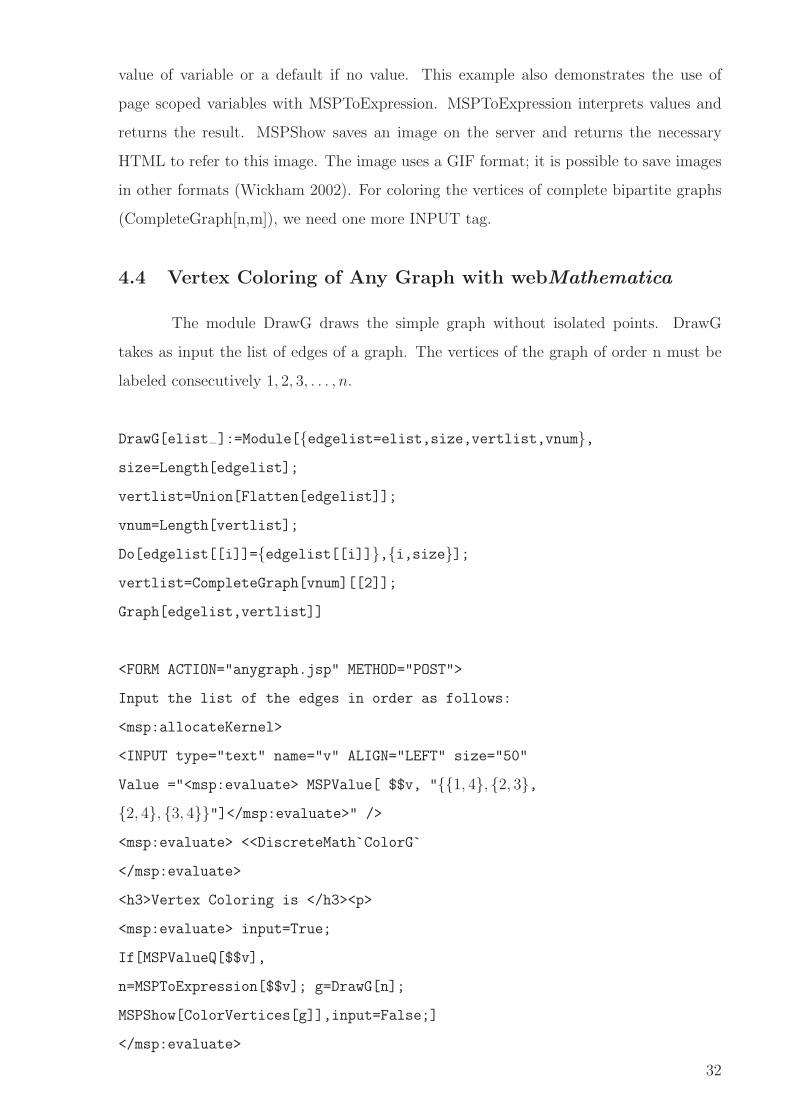
In the vertex.jsp, there are two <INPUT> tags: the first one allows the user of
the page to enter the number of the vertices in the graph, and the second specifies a
button that, when pressed, will submit the FORM. When the FORM is submitted, it
will send information from INPUT elements to the URL specified by the ACTION at-
tribute; in this case, the URL is the same MSP. Information entered by the user is sent
to a Mathematica session and assigned to a Mathematica symbol (see Figure 4.4). Addi-
tionally, the Mathlets refer to Mathematica functions that are not in standard usage. In
this example some Mathematica commands; If, Table, Flatten, Position, VertexColoring,
CompleteGraph, Cycle, Wheel, ShowGraph, Highlight, ChromaticNumber, True, False
and some mathematical operations are used by the Mathlets. The name of the symbol
is given by prepending $$ to the value of the NAME attribute. MSPValue, MSPBlock,
MSPShow, MSPToExpression are webMathematica commands. MSPValue returns the
31
value of variable or a default if no value. This example also demonstrates the use of
page scoped variables with MSPToExpression. MSPToExpression interprets values and
returns the result. MSPShow saves an image on the server and returns the necessary
HTML to refer to this image. The image uses a GIF format; it is possible to save images
in other formats (Wickham 2002). For coloring the vertices of complete bipartite graphs
(CompleteGraph[n,m]), we need one more INPUT tag.
4.4 Vertex Coloring of Any Graph with webMathematica
The module DrawG draws the simple graph without isolated points. DrawG
takes as input the list of edges of a graph. The vertices of the graph of order n must be
labeled consecutively 1, 2, 3, . . . , n.
DrawG[elist−]:=Module[{edgelist=elist,size,vertlist,vnum},
size=Length[edgelist];
vertlist=Union[Flatten[edgelist]];
vnum=Length[vertlist];
Do[edgelist[[i]]={edgelist[[i]]},{i,size}];
vertlist=CompleteGraph[vnum][[2]];
Graph[edgelist,vertlist]]
<FORM ACTION="anygraph.jsp" METHOD="POST">
Input the list of the edges in order as follows:
<msp:allocateKernel>
<INPUT type="text" name="v" ALIGN="LEFT" size="50"
Value ="<msp:evaluate> MSPValue[ $$v, "{{1, 4}, {2, 3},
{2, 4}, {3, 4}}"]</msp:evaluate>" />
<msp:evaluate> <<DiscreteMath`ColorG`
</msp:evaluate>
<h3>Vertex Coloring is </h3><p>
<msp:evaluate> input=True;
If[MSPValueQ[$$v],
n=MSPToExpression[$$v]; g=DrawG[n];
MSPShow[ColorVertices[g]],input=False;]
</msp:evaluate>
32
The Chromatic Number of the given graph is
<msp:evaluate>
kn=ChromaticNumber[g]
</msp:evaluate></p>
<INPUT TYPE="Hidden" NAME="formNo" VALUE="1">
<INPUT TYPE="Submit"NAME="taskValue"
VALUE="Color the graph’s vertices" >
</msp:allocateKernel>
</form>
Figure 4.1: Vertex Coloring of a Graph with webMathematica
4.5 Generating Graphs with webMathematica
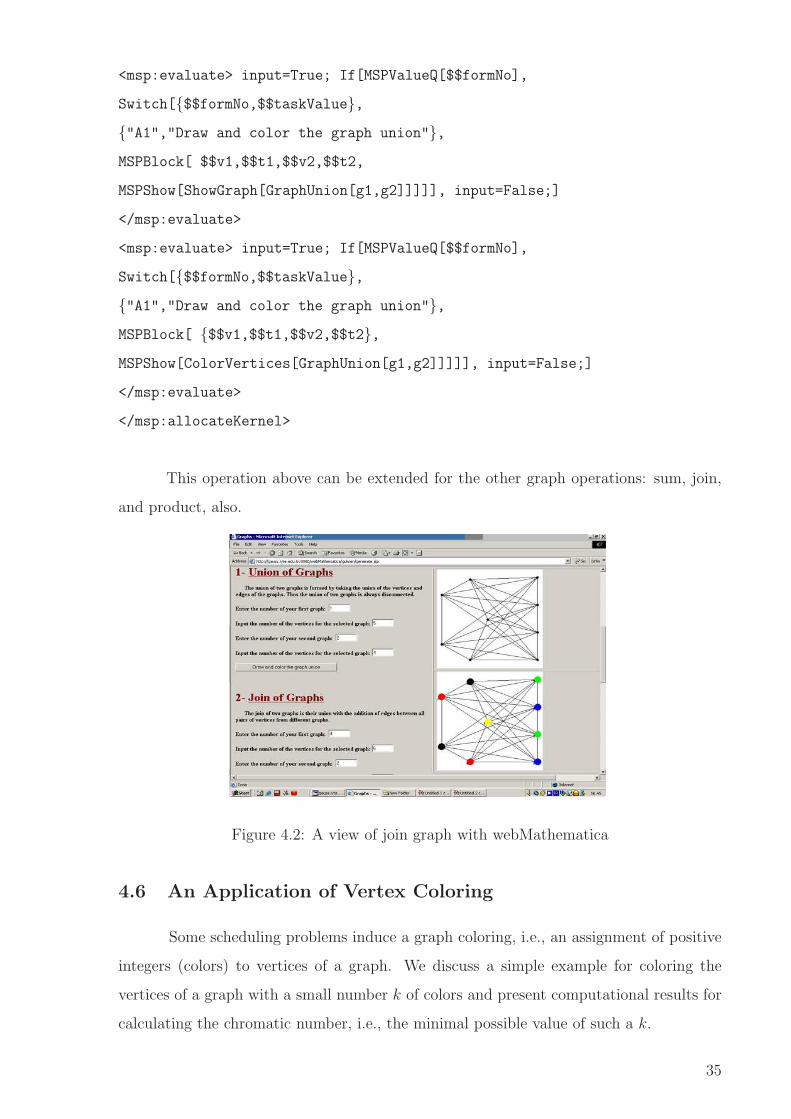
This section presents operations that build graphs from other graphs. The most
important operations on graphs are sum, union, join, and product of graphs. We will
use these operations with the common graphs; complete graph, random tree, wheel, and
cycle.
The join of two graphs is their union with the addition of edges between all pairs
of vertices from different graphs. To take the join of two graphs the user should enter
the number of the graphs and their vertex numbers into the boxes then he/she sees the
join of those graphs and also its proper vertex coloring. The user should enter “1” for the
complete graph, for random tree “2”, for wheel “3”, for cycle “4”.
33
We use some commands in the ColorG package to color the vertices of the
generated graphs and to give web-based examples with webMathematica as follows:
<FORM ACTION="generate.jsp" METHOD="POST">
<p>Please select one of the following graphs and
input into the box:(1,2,3,or 4) </p> <p>1-CompleteGraph,</p>
<p>2-RandomTree, </p> <p>3-Wheel,</p> <p>4-Cycle</p>
<msp:allocateKernel>
<FORM ACTION="generate.jsp" METHOD="POST">
<font color="#800000" size="6">1- <u>Union of Graphs</u></font>
<INPUT type="text" name="t1" ALIGN="LEFT" size="6" value="
<msp:evaluate> MSPValue[$$t1,"1"]</msp:evaluate>" />
Input the number of the vertices for the selected graph:
<INPUT type="text" name="v1" ALIGN="LEFT" size="6"
value="<msp:evaluate> MSPValue[$$v1,"5"]</msp:evaluate>" />
Enter the number of your second graph:
<INPUT type="text" name="t2" ALIGN="LEFT" size="6"
value="<msp:evaluate> MSPValue[$$t2,"2"]</msp:evaluate>" />
Input the number of the vertices for the selected graph:
<INPUT type="text" name="v2" ALIGN="LEFT" size="6"
value="<msp:evaluate> MSPValue[$$v2,"4"]</msp:evaluate>" />
<msp:evaluate> MSPBlock[{$$v1,$$t1},
Which[$$t1==1, g1=CompleteGraph[$$v1];,
$$t1==2, g1=RandomTree[$$v1];,
$$t1==3, g1=Wheel[$$v1];,
$$t1==4, g1=Cycle[$$v1];]]
</msp:evaluate>
<msp:evaluate> MSPBlock[{$$v2,$$t2},
Which[$$t2 == 1, g2=CompleteGraph[$$v2];,
$$t2 == 2, g2=RandomTree[$$v2];,
$$t2 == 3, g2=Wheel[$$v2];,
$$t2 == 4, g2=Cycle[$$v2];]]
</msp:evaluate>
</FORM>
34
<msp:evaluate> input=True; If[MSPValueQ[$$formNo],
Switch[{$$formNo,$$taskValue},
{"A1","Draw and color the graph union"},
MSPBlock[ $$v1,$$t1,$$v2,$$t2,
MSPShow[ShowGraph[GraphUnion[g1,g2]]]]], input=False;]
</msp:evaluate>
<msp:evaluate> input=True; If[MSPValueQ[$$formNo],
Switch[{$$formNo,$$taskValue},
{"A1","Draw and color the graph union"},
MSPBlock[ {$$v1,$$t1,$$v2,$$t2},
MSPShow[ColorVertices[GraphUnion[g1,g2]]]]], input=False;]
</msp:evaluate>
</msp:allocateKernel>
This operation above can be extended for the other graph operations: sum, join,
and product, also.
Figure 4.2: A view of join graph with webMathematica
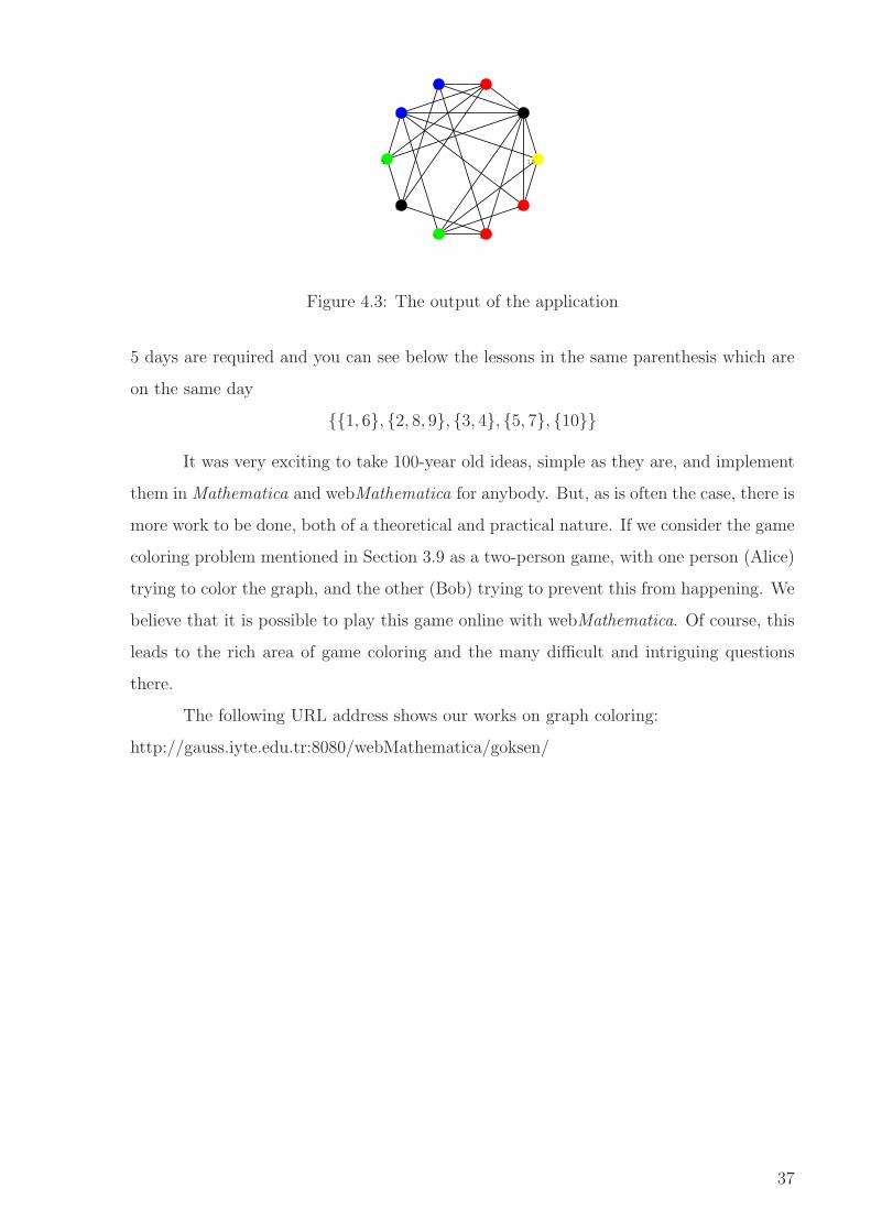
4.6 An Application of Vertex Coloring
Some scheduling problems induce a graph coloring, i.e., an assignment of positive
integers (colors) to vertices of a graph. We discuss a simple example for coloring the
vertices of a graph with a small number k of colors and present computational results for
calculating the chromatic number, i.e., the minimal possible value of such a k.
35
Draw up an examination schedule involving the minimum number of days for the
following problem:
Set of students: S1, S2, S3, S4, S5, S6, S7, S8, S9
Examination subjects for each group: {algebra, real analysis, and topology}, {algebra,
operations research, and complex analysis }, {real analysis, functional analysis, and
topology }, {algebra, graph theory, and combinatorics }, {combinatorics, topology, and
functional analysis }, {operations research, graph theory, and coding theory }, {operations
research, graph theory, and number theory }, {algebra, number theory, and coding
theory }, {algebra, operations research, and real analysis}.
Let S be a set of students, P = {1, 2, 3, 4, 5, 6, 7, 8, 9, 10} be the set of examinations
respectively algebra, real analysis, topology, operational research, complex analysis,
functional analysis, graph theory, combinatorics, coding theory, and number theory. S(p)
be the set of students who will take the examination p ∈ P . Form a graph G = G(P,E),
where a, b ∈ P are adjacent if and only if S(a) ∩ S(b) 6= Ø. Then each proper vertex col-
oring of G yields an examination schedule with the vertices in any color class representing
the schedule on a particular day. Thus χ(G) gives the minimum number of days required
for the examination schedule. The Mathematica commands for this solution are as follows:
k = Input["Input the number of the students"];
S = Table[Input["Input number of the lessons which the student will
choose"], k];
b = Union[Flatten[Table[KSubsets[S[[i]], 2], i, k], 1]];
ColorVertices[t = DrawG[b]];
h = VertexColoring[t]; d=ChromaticNumber[t];
Print[d"days are requared and you can see below the lessons in the same
paranthesis which are on the same day"]
Table[Flatten[Position[h, i], 2], i, Max[h]]
36
1
23
4
5
6
7 8
9
10
Figure 4.3: The output of the application
5 days are required and you can see below the lessons in the same parenthesis which are
on the same day
{{1, 6}, {2, 8, 9}, {3, 4}, {5, 7}, {10}}
It was very exciting to take 100-year old ideas, simple as they are, and implement
them in Mathematica and webMathematica for anybody. But, as is often the case, there is
more work to be done, both of a theoretical and practical nature. If we consider the game
coloring problem mentioned in Section 3.9 as a two-person game, with one person (Alice)
trying to color the graph, and the other (Bob) trying to prevent this from happening. We
believe that it is possible to play this game online with webMathematica. Of course, this
leads to the rich area of game coloring and the many difficult and intriguing questions
there.
The following URL address shows our works on graph coloring:
http://gauss.iyte.edu.tr:8080/webMathematica/goksen/
37
REFERENCES
Appel, K.I. and Haken, W., 1976. “Every planar map is four-colorable”, Bull. Amer.
Math. Soc., No. 82, pp. 711-712.
Balakrishnan, R. and Ranganathan, K., 2000. A Textbook of Graph Theory, (Springer-
Verlag).
Balakrishnan, V.K., 1997. Schaum’s Outline of Theory and Problems of Graph Theory,
(McGraw-Hill Companies, Inc.).
Berge, C., 1973. Graphs and Hypergraphs, (North-Holland Publishing Company).
Birkhoff, G.D., 1912. “A determinant formula for the number of ways of coloring a map”,
Ann. of Math.. No. 14, pp. 42-46.
Bodlaender, H.L., 1991. “On the complexity of some coloring games”, Lecture Notes in
Computer Science. No. 484, pp. 30-40.
Bondy, J.A. and Murty, U.S.R., 1985. Graph Theory with Applications, (Elsevier Science
Publishing Co., Inc.).
Buckley, F. and Haray, F., 1990. Distance in Graphs, (Addison-Wesley Publishing
Company).
Chartrand, G. and Lesniak, L., 2000. Graphs & Digraphs, (Chapman & Hall / CRC).
Faigle, U., Kern, U., Kierstead, H. and Trotter, W.T., 1993. “On the game chromatic
number of some classes of graphs”, Ars Combinatorica, No. 35, pp. 143-150.
Gibson, A., 1994. Algorithmic Graph Theory, (Cambridge University Press).
Gross, J. and Yellen, J., 1999. Graph Theory and Its Applications, (CRC Press).
Guan, D., 1999. “The game chromatic number of outerplanar graphs”, Journal of Graph
Theory, No. 30, pp. 67-70.
Henning, M.A., 1997. “Research in Graph Theory”, South African Journal of Science,
No. 93, pp. 15-23.
Kierstead, H. and Trotter, W.T., 1994. “Planar graph coloring with an uncooperative
partner”, J. Graph Theory 18, No. 6, pp. 569-584.
Lovasz, L., 1975. “Three short proofs in Graph Theory”, J. Combinatorial Theory, No.,
19, pp. 111-113.
Melkinov, L.S., and Vizing, V.G., 1969. “New proof of Brooks’ Theorem”, J. Combina-
torial Theory, No. 7, pp. 289-290.
Pemmaraju, S. and Skiena, S., 2003. Computational Discrete Mathematics-Combinatorics
and Graph Theory with Mathematica, (Cambridge University Press).
38
Read, R.C., 1968. “An introduction to chromatic polynomials”, J. Combinatorial Theory,
No. 4, pp. 52-71.
Skiena, S., 1990. Implementing Discrete Mathematics: Combinatorics and Graph Theory
with Mathematica, (Addison-Wesley Publishing Co.)
Szekeres, G. and Wilf, H.S., 1968. “An inequality for the chromatic number of a graph”,
J. Combinatorial Theory, No. 4, pp. 1-3.
Thulasiraman, K. and Swamy, M.N.S., 1992. Graphs:Theory and Algorithms, (John Wiley
& Sons, Inc.).
Tutte, W.T., 1970. “On chromatic polynomials and the golden ratio”, J. Combinatorial
Theory, No. 9, pp. 289-296.
Ufuktepe, U., 2003. “An Application with webMathematica”, Lecture Notes in Computer
Science , No. 2657, pp. 774-780.
Ufuktepe, U. and Bacak, G., “Applications of Graph Coloring”, Future Generation
Computer Systems, (to appear).
Ufuktepe, U., Bacak, G. and Beseri, T., 2004. “Graph coloring with webMathematica”,
Lecture Notes in Computer Science , No. 3039, pp. 376-381.
Ufuktepe, U., Beseri, T. and Bacak, G., 2004. “Graph Theory with webMathematica”,
Proceedings of the 6th International Mathematica Symphosium.
Vizing, W.G., 1963. “The Cartesian product of graphs”, Vyc. Sis., No. 9, p. 30-43.
Welsh, D.J.A. and Powel, M.B., 1967. “An upper bound for the chromatic number of a
graph and its application to timetabling problems”, Computer J., No. 10, pp. 85-87.
West, D.B., 2001. Introduction to Graph Theory, (Prentice Hall, Inc.).
Wickham, T., 2002. webMathematica A User Guide, (Wolfram Research Inc.).
Wilson, R.J., 1996. Introduction to Graph Theory, (Pearson Education Ltd.).
Wolfram, S., 1996. The Mathematica Book, (Cambridge Univ. Press).
39