vertical relations: double marginalization, price negotiation and integration · vertical pricing...

Vertical Relations: Double Marginalization, PriceNegotiation and Integration

Jean-Francois HoudeCornell University & NBER

October 17, 2016

Vertical Relations 1 / 41

Introduction: Vertical Contracting

Goal: Solve an externality problem between downstream andupstream firms

I Agency problem: Unmeasurable service qualityI Pricing: Double marginalizationI Upstream competition: Exclusion of rival suppliersI Under-investment: Incomplete contracting

Double marginalization: Retailer does not internalize the loss inrevenue from setting prices above cost.

Legal restrictions:I Resale-price maintenance (RPM) is illegal in the U.S.I Wholesale price discrimination is illegal only if judged anticompetitive

(almost never prosecuted)I Tie-in and exclusive territories are judge by a rule of reason (technically

illegal)I Vertical mergers are rarely prosecuted by the federal agencies

Vertical Relations Double Marginalization 2 / 41

Double Marginalization: Basic Model

Linear pricing contract: Manufacturer sets wholesale price wI Downstream firm (with market-power):

maxp

(p − w)D(p)↔ D(p) + D ′(p)(p − w) = 0

I Upstream firm (monopolist):

maxw

(w − c)D(p(w))↔ D(p(w)) + D ′(p(w))(w − c)p′(w) = 0

I Key result: As long as w > c , p∗ > pVI and q∗ < qVI . Why?F Downstream firm fails to internalize the profit loss to the manufacturer

associated with selling fewer units than qVI .

Remedies:I Two-part tariff contract (i.e. franchising)

w = c and F = (pVI − c)qVI

I Resale-price maintenanceI Minimum quantity contractsI Vertical integration


Testing for Double MarginalizationSource: Villas-Boas (2007)

Data: The market for Yogurt in a Midwestern cityI Source: IRII Market-structure: 5 Manufacturers × 3 Retailers = 43 productsI Sample: Product characteristics and sales over 104 weeks

Mixed-logit demand (omitting time dimension):

uij = xjβi − αipj + ξj + εij ,(βiαi

)=

(βα

)+ DiΓ + νiΣ

where j ∈ 0, 1, . . . ,N, N is the number of brands × stores, and Di

is a vector of demographic characteristics (age and income), andνi ∼ N(0, 1).

The demand parameters are estimated as in Nevo (2001).I Instruments: Aggregate cost-shocks × product FEs (pretty weak...)


Vertical Pricing

Assumption: Manufacturers are allowed to charge different wholesaleprices for each retailer/product combination (i.e. wj)

Notation: (again omitting the time dimension)I Ωr : Ownership matrix at the retail levelI Ωw : Manufacturer ownership matrix (i.e. brands)I ∆r : Retail demand own and cross price derivative (i.e. ∆r

jk = ∂sk/∂pj)I ∆w : Wholesale demand own and cross derivative (i.e. ∆w

jk = ∂sk/∂wj)I Λ: Retail equilibrium pass-through matrix (i.e. Λkj = dpk/dwj)

Identity: Manufacturer perceived demand slope depends on theretailers’ anticipated pricing decision

∆wjk = ∂sk/∂wj =

N∑l=1

∂sk∂pl

dpldwj

, or ∆w = ΛT∆r

Timing: Manufacturers set wholesale prices, and retailers determineretail prices knowing the entire vector of wholesale price


Vertical Contract 1: Linear Pricing

Retail supply relation:

(pj) : sj +∑k

Ωrjk

∂sk∂pj

(pk − wk − c rj ) = 0↔ pj = c rj + wj + (Ωr ·∆r )−1j,. s

Wholesale supply relation:

(wj) : sj +∑k

Ωwjk

∂sk∂wj

(wk − cwk ) = 0, where∂sk∂wj

=N∑l=1

∂sk∂pl

dpldwj

↔ wj = cwj +[Ωw ·

(ΛT∆r

)]−1

j,.s

Equilibrium pass-through (differentiating retailers’ FOC):

(wf ) :N∑l=1

[∂sj∂pl

+∑k

Ωrjk∂2sk∂pj∂pl

(pk − wk) + Ωrjk∂sl∂pj

]︸︷︷︸

g(j,l)

dpldwf− Ωr

jf∂sf∂pj︸︷︷︸

h(j,f )

= 0

↔ Λ = G−1H


Vertical Pricing (continued)

Model 2: Non-linear pricingI Manufacturer sets wj = cwj and charges a fixed-fee fee Fj (does not

affect prices):

(pj) : sj+∑k

Ωrjk

∂sk∂pj

(pk−cwj −c rj ) = 0↔ pj = c rj +cwj +(Ωr ·∆r )−1j,. s

I Alternatively, retailer set pj = wj + c r and manufacturer transferspayment to retailer:

(wj) : sj +∑k

Ωwjk

∂sk∂wj

(wk − cwk ) = 0

↔ sj +∑k

Ωwjk

∂sk∂pj

(pk − c rk − cwk ) = 0

I Note: This last FOC, is equivalent to the one used in BLP and Nevo.


Vertical Pricing (continued)

Alternative models: Partial collusion and linear pricingI Downstream collusion: Ωr = OI Upstream collusion: Ωw = OI Monopoly pricing and vertical integrationI Etc.

Conclusion: Even if we do not observe wjt , alternative verticalpricing models imply different supply relations equations

pjt = xjtγ + λw

[Ωwt ·(

ΛTt ∆r

t

)]−1

j ,.st + λr

[Ωrt ·∆r

t

]−1

j ,.st + ωjt

where xjtγ + ωjt = cwjt + c rjt , and Θ =λw , λr , Ω

r , Ωw

represent

alternative vertical conduct assumptions.

Identification: This supply relation corresponds to a non-linear IVproblem. To identify Θ, we need valid/relevant instruments.

I Missing from the paper...I What would be a good IV?


Results: Estimated marginal cost


Results: Non-Nested Hypothesis Tests

Takeaway: The data is consistent with models without doublemarginalization

Cause for concerns: The moment conditions are not able to distinguishbetween the Monopoly and Bertrand-Nash models...


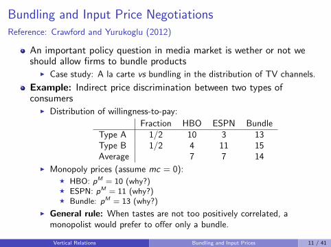
Bundling and Input Price NegotiationsReference: Crawford and Yurukoglu (2012)

An important policy question in media market is wether or not weshould allow firms to bundle products

I Case study: A la carte vs bundling in the distribution of TV channels.

Example: Indirect price discrimination between two types ofconsumers

I Distribution of willingness-to-pay:

Fraction HBO ESPN BundleType A 1/2 10 3 13Type B 1/2 4 11 15Average 7 7 14

I Monopoly prices (assume mc = 0):F HBO: pM = 10 (why?)F ESPN: pM = 11 (why?)F Bundle: pM = 13 (why?)

I General rule: When tastes are not too positively correlated, amonopolist would prefer to offer only a bundle.

Vertical Relations Bundling and Input Prices 11 / 41

What if upstream firms have positive bargaining power?

The previous example assumes that the downstream monopolist canmake a take-it-or-leave-it offer to HBO and ESPN (and MC = 0).

Timing:1 Distributor simultaneously negotiate with HBO and ESPN over cost2 Distributor sets prices and decide to bundle or not3 Demand and profits are realized

In the two-types example, bargaining is purely about how to split thesurplus (i.e. pm is independent of wj)

“Nash-in-Nash” multi-lateral bargaining over the bundle (Horn andWollinsky (1988)):

I Nash bargaining fixing w−j

maxwj

((pm − wj − w−j)× D)β (D × (wj − 0))1−β

↔ wj = (1− β)pm − (1− β)w−j

I Simultaneous Nash equilibrium (symmetric): wj = w−j = pm (1−β)2+β


What if upstream firms have positive bargaining power?

In this example, if upstream firms have sufficient bargaining power(i.e. low β), bundling is no longer the most profitable option.

The results crucially depend on: (i) heterogeneity and correlation intaste, and (ii) profitability the partial versus full coverage (i.e. outsideoption).


The TV Industry Supply Chain


Bundling and Input Prices in TV Markets

Market structure:I Cable distributors typically offer multiple tiers bundlesI Content providers control multiple TV channels (e.g. Disney, Time

Warner, etc)I Input prices vary across distributors (f ) and channels (c): τfc

Structure of the problem:I Stage 1: Estimation of the distribution of WTP for channelsI Stage 2: Optimal bundle composition and bundling costI Stage 3: Estimation of bargaining parameter

Main data-sets:I Factbook: Local cable market-level data on the composition of

bundles, prices, market shares, ownership.I Economics of basic cable networks: Channel-level data on cost and

revenue (τ ’s).I Viewership: Channel ratings per DMA/period + household survey on

hours spent per channel


Estimation of the distribution of WTP for channels

Indirect utility for bundle j :

uijm =∑c∈Cj

γic log(1 + t∗ijc)

︸︷︷︸v∗ijm

+xjmγ + αipjm + ξjm + εijm

= δjm + µijm + εijm

Time allocation:

t∗i = arg maxtic∑c∈Cj

γic log(1 + tic), s.t.∑c

tic < T

Parametrization of channel tastes:

γic =

0 With probability: ρc(zi )

ziβ + νic With probability: 1− ρc(zi )

where νi = (νi1, . . . , νiC ) ∼ Exp(V ,Σ).


Estimation of the distribution of WTP for channels

Aggregate demand takes the standard mixed-logit form:

σjm(δm,Fm; θ) =

∫exp(δjm + µijm(zi , νi )

1 +∑

k exp(δkm + µikm(zi , νi )dΦ(νi ;V ,Σ)dFm(zi )

The parameters of the model are estimated by matching viewershipand market shares data

I Shares of consumers with positive viewership for channel c (given zi )I Average time spent watching channel c (given zi )I Covariance between ratings of channel c and ziI Conditional market shares of cable and satellite (given zi )I etc.

This is similar to Bayer, Ferreira, and McMillan (2007). The keydifference is that we use usage intensity measure from surveys toidentify the distribution of tastes (rather than observed choices).


Estimation of Channel Input Costs

Challenges:I The data only contains information on average channel input costs

across distributors: τc = E (τfc).I Since channels are only sold through bundles, the price that distributer

f charges for each bundle does not reveal the cost of individualchannels (only the marginal cost of the bundle)

Solution: Parametrize input cost function as,

τfc = (η1 + η2τc) exp(φ1Nb. Subscribersf + φ2Ownership Sharefc)

Equilibrium restriction: Bundle prices

∂Πfm(bm, pm, τ)

∂pjm=∑j∈Bfm

pjm −∑c∈Cjm

τfc

∂σjm(pm)

∂pkm+ σkm(pm) = 0

MCjm(pm) =∑c∈Cj

τfc = − (∆× Ω)−1j ,· σm


Estimation of Channel Input Costs (continued)

Equilibrium restriction: Bundle compositionI Value of offering bundle bfm in market m:

Vfm(bfm, b−fm, τ) = Πfm ((bfm, b−fm), (pfm, p−fm), τ) + Errorb,fm

I If bundles and prices are chosen simultaneously, Nash-eqlb. implies:

Vfm(bfm, b−fm, τ) > Vfm(b′fm, b−fm, τ)↔

Πfm ((bfm, b−fm), (pfm, p−fm), τ)− Πfm

((b′fm, b−fm), (p′fm, p−fm), τ

)︸︷︷︸=∆Πfm(b,b′)

> Errorbb′,fm

I Assumption: Mean zero error expressed in deviation

E (Errorbb′,fm + Errorb′b,fm′) = 0

I This implies the following moment inequality (see Pakes et al. (2006)):

E (∆Πfm(b, b′, τ) + ∆Πfm′(b′, b, τ)) ≥ 0, if τfc = τ 0fc ,∀(f , c).


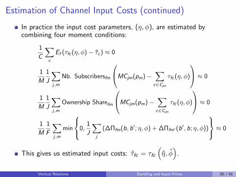
Estimation of Channel Input Costs (continued)

In practice the input cost parameters, (η, φ), are estimated bycombining four moment conditions:

1

C

∑c

Ef (τfc(η, φ)− τc) ≈ 0

1

M

1

J

∑j,m

Nb. Subscribersfm

MCjm(pm)−∑c∈Cjm

τfc(η, φ)

≈ 0

1

M

1

J

∑j,m

Ownership Sharefm

MCjm(pm)−∑c∈Cjm

τfc(η, φ)

≈ 0

1

M

1

F

∑j,m

min

0,1

J

∑j

(∆Πfm(b, b′; η, φ) + ∆Πfm′(b′, b; η, φ))

≈ 0

This gives us estimated input costs: τfc = τfc

(η, φ)

.


Estimation of the Bargaining Parameter(s)

Question: Are the estimated input costs consistent with buyer orseller bargaining power?

Consider a distributer, f , present in only one market, negotiating witha conglomerate, k , of channels (e.g. ABC/Disney)

Holding fixed the input cost negotiated with otherdistributers/conglomerates, the vector τfk is a solution to thefollowing Nash-Bargaining problem:

maxτfk

(Πf (τfk , τf ,−k)− Πf (∞, τf ,−k))ξfk

(Πk(τfk , τ−f ,k)− Πk(∞, τ−f ,k))1−ξfk

Threat points: Πf (∞, τf ,−k) is the profit of distributer f withoutthe channels offered by k , and Πk(∞, τ−f ,k) is the conglomerate’sprofits if cannot distribute its channels to firm f .



Since we have estimated all the τfc ’s, the disagreement payoffs (orthreat points) can be calculated from the data.

If the τfc ’s are generated in equilibrium they must satisfy the followingFOC:

ξfk

Πf − Π−kf

∂Πf

∂τfc=

1− ξfkΠk − Π−fk

∂Πk

∂τfc, ∀c ∈ Ck

The bargaining weight parameters can therefore be estimated byfinding the value of ξfk that minimizes the sum of square residualbetween τfc and τfc(ξ).

I Note: Alternatively, there should be a way of inverting the above FOCto recover an estimate of ξfk . See Grennan (2013).

In practice, the paper “solves” each bargaining game independently(holding fixed τ−f ), and finds the ξfk that fits the data best.

I This implies solving a simplified version of the downstream game foralternative values of τfc ’s.

I What about bundle composition?



Questions:I The bargaining parameters are the “residuals” that rationalize the

estimated τfc ’s, given the functional form assumption for τfc(η, φ) andthe assumption of firms’ threat points.

I What do we know about the dispersion of τfc in practice? What aboutfirms’ threat points (i.e. leverage)? What if negotiation was sequential?

I This is an important area of research.


Estimated distribution of channel WTPs


Estimated input cost functionτfc = (η1 + η2τc) exp(φ1Nb. Subscribersf + φ2Ownership Sharefc)

Is this a good model of vertical integration?


Estimated bargaining parameters for large conglomerates


Counter-Factual Simulation Results: ALC vs Bundling


What is the effect of upstream mergers?Reference: Gowrisankaran, Nevo, and Town (2015)

So far we have studied mergers in markets in which buyers areprice-takers

I Workhorse model: Multi-product Bertrand-Nash equilibrium

This framework is not appropriate to study mergers betweenoligopolists

I If buyers have full bargaining power, upstream mergers will have zeroeffect on prices

I If sellers have full bargaining power, downstream mergers will have zeroeffect of prices.

Mergers in health-care markets:I The hospital industry is responsible for the largest number of horizontal

merger litigation by federal agencies (first success in 2011!)I At the same time, private health insurance markets have become

increasing concentrated (Dafny et al. (2012))

Vertical Relations Mergers with negotiated input prices 28 / 41

Fact 1: Insurance Concentration and PremiumsReference: Dafny et al. (2012)


Fact 2: Dispersion of Discounts and Buyer PowerReference: Sorensen (2003)


Model: Bargaining Between Hospitals and MCOs

Market structure:I J hospitals and M managed-car organizations (MCOs).I MCOs offer their enrollees access to a network of hospitals: Nm (fixed).

Objectives:I MCO: Maximize the weighted sum of consumer surplus of its enrollees

net of payments to hospitals (pmj).

Vm(Nm, pm) = E

[τCSi (Nm, pm)−

∑j∈Nm

(1− ci )fipmjσij

∣∣∣∣∣m(i) = m

]

where τ is welfare weight, CSi is the surplus of consumer i (in $), fi isthe probability being sick, and ci is the copay % (fixed).

I Hospitals: Maximize expected profits

Πsm(Nm, pm) =∑j∈Js

qmj(Nm, pm)(pmj −mcmj)

where qmj is the number of patients “send” from MCO m to hospitalj , pmj is the hospital cost charged to MCO m, and mcmj is themarginal cost of serving patients from MCO m.



Assumption: Constant marginal cost

mcmj = vmjγ + ωmj

where vmj is a vector of hospital and MCO characteristics, and ωmj isan unobserved relation-specific cost shock.

Threat points:I MCO: If negotiation fails, insurees do not have access to the hospital

in network Ns

Vm(Nm\Js , pm) = E

τCSi (Nm\Js , pm)−∑

j∈Nm\Js

(1− ci )fipmjσij

∣∣∣∣∣m(i) = m

I Hospitals: Because of the constant marginal cost assumption, the

disagreement profits are zero



Nash-in-Nash bargaining:I Hold fixed the negotiated prices with other networks: pmjj /∈Js

.I Input prices solve the following Nash-Bargaining problem:

maxpmj :j∈Js

[Vm(Nm, pm)− Vm(Nm\Js , pm)]bms [Πsm(Nm, pm)]1−bms

I Nash equilibrium conditions conditions:

−bms

Vm(Nm, pm)− Vm(Nm\Js , pm)

∂Vm(Nm, pm)

∂pmj=

(1− bms)

Πsm(Nm, pm)

∂Πsm(Nm, pm)

∂pmj

for all j ∈ Ns , s and m bilateral negotiation pairs.

Note: If bms = 0, ∂Πsm(Nm,pm)∂pms

= 0 (i.e. Bertrand-Nash condition).


Inferring Marginal Cost From Input Prices

Recall: ∂Πsm(Nm,pm)∂pmj

= qmj +∑

k∈Ns

∂qmk∂pmj

(pmk −mcmk)

Rearranging the NB FOC:

−bms

Vm(Nm, pm)− Vm(Nm\Js , pm)

∂Vm(Nm, pm)

∂pmj︸︷︷︸=−bms

AB

=(1− bms)

Πsm(Nm, pm)

∂Πsm(Nm, pm)

∂pmj

↔ q + Ω(p −mc) = −∆(p −mc)↔ p −mc = −(Ω + ∆)−1q

where q is |Ns | × 1 vector, Ωj ,k = ∂qmk/∂pmj , and∆j ,k = (bms/(1− bms))(A/B)qmk .

Therefore, conditional on bms , the marginal cost of pair (m, s) can beinferred from observed input prices and quantities.

This is different from Crawford and Yurukoglu (2012): Marginal costof channels were assumed to be zero, and the bargaining weights werethe model “residuals”.


How the bargaining leverage of both parties affect prices?

Buyer leverage: AB =

∂Vms∂pmj

Vms−V−ms

I The bargaining leverage of the MCOs is determined by their ability of“steering” patients away from high-cost hospital, due to the co-pay(numerator)

I The effect of loosing hospital network Ns on consumer welfare(denominator)

I If consumers are not sensitive to prices (and/or τ = 0), hospitals willbe able to charge higher costs (everything else being equal)

Seller leverage:∂Πsm/∂pmj

Πsm

I Because hospitals have constant MC, size does not directly affect theirleverage.

I Hospitals with larger networks have more leverage:F Standard business stealing effect: ∂Πsm/∂pmj

F Lowers the leverage of MCOs: Large welfare loss Vms − V−ms

Upstream mergers: Standard business-stealing internalization +Relative bargaining leverage change.


Estimation: Demand and Consumer SurplusHospital choice: Consumer with hospital netowork Nm(i)

I Conditional of a realized illness d ∈ 1, . . . ,D:

maxj∈Nm(i)

xijdβ − αcidwdpm(i),j + εijd

where cid is co-payment, and wd is a disease weight.I The base price, pmj , is the outcome of the negotiation between the

MCO and hospital network.Aggregate demand from MCO m:

qmd =∑i

1(m(i) = m)∑d

fidexp(xijdβ − αcidwdpm(i),j)∑

k∈Nm(i)exp(xikdβ − αcidwdpm(i),k)

Expected utility:

Wi (Nm, pm) =∑d

fid ln

∑k∈Nm(i)

exp(xikdβ − αcidwdpm(i),k)

From this, we can compute consumers’ WTP for hospital network Js :

WTPims = Wi (Nm, pm)−Wi (Nm\Js , pm)


Estimation: Demand and Consumer Surplus

Data source:I Payor data: Administrative claims data for four MCOs in VirgniaI Discharge data: Virginia health information

Price: cmpmj

I Regression of the disease weighted amount paid to hospital j separatelyfor each MCO and year:

TPijt/wd = µj + ziγ + eijt

I Base price = Average predicted paymentI Similar regression is used to calculate expected co-insurance rate (%)

Additional control variables:I Hosptial/Year FEI Distance between individuals and hospitals

Estimation: MLE of observed hospital choices conditional on illnessI Identification: Exogenous variation in prices due to negotiated prices

and coinsurance (across payors)


Demand Elasticity


Estimation: Marginal Cost and Bargaining Power

The bargaining model implies the following pricing equation:

pms = mcms − (Ωms + ∆ms)−1qms

where q is |Ns | × 1 vector, Ωj ,k = ∂qmk/∂pmj , and∆j ,k = (bms/(1− bms))(A/B)qmk .

This leads to a non-linear IV regression (just like BLP):

pmj = vmjγ + g(qms , pms ; b, τ) + ωmj

where vmj includes MCO, year and hospital FEs.

Identification:I Conditional of hospital and MCO FEs, the IVs must shift the relative

leverage within hospital networks or within MCOs.I Zmj : Predicted WTP and quantity evaluated at the average prices.


Marginal Cost and Bargaining Power Estimates


Merger Simulation


Bayer, P., F. Ferreira, and R. McMillan (2007).A unified framework for measuring preferences for schools and neighborhoods.Journal of Political Economy 115(5), 588–638.

Crawford, G. S. and A. Yurukoglu (2012).The welfare effects of bundling in multichannel television markets.American Economic Review 102(2), 643–85.

Dafny, L., M. Duggan, and S. Ramanarayanan (2012).Paying a premium on your premium? consolidation in the us health insurance

industry.American Economic Review 102(2), 1161–1185.

Gowrisankaran, G., A. Nevo, and R. Town (2015).Mergers when prices are negotiated: Evidence from the hospital industry.American Economic Review 105, 172–203.

Grennan, M. (2013).Price discrimination and bargaining: Empirical evidence from medical devices.American economic Review 103(1), 145–177.

Horn, H. and A. Wollinsky (1988).Vertical Relations References 41 / 41

Bilateral monopolies and incentives for merger.Rand Journal of Economics 19(3), 408–419.

Nevo, A. (2001).Measuring market power in the ready-to-eat cereal industry.Econometrica 69(2), 307.

Pakes, A., J. Porter, K. Ho, and J. Ishii (2006, November).Moment inequalities and their application.

Sorensen, A. T. (2003, December).Journal of industrial economics.Insurer-Hospital Bargaining: Negotiated Discounts in Post-Deregulated

Connecticut 51(4), 469–490.

Villas-Boas, S. B. (2007).Vertical relationships between manufacturers and retailers: Inference with

limited data.Review of Economic Studies.

Vertical Relations References 41 / 41

vertical relations: double marginalization, price negotiation and integration · vertical pricing...

Documents