1

Vertical Scaling in Value-Added Models for Student

Learning Derek Briggs

Jonathan WeeksEd Wiley

University of Colorado, Boulder

Presentation at the annual meeting of the National Conference on Value-Added Modeling. April 22-24, 2008. Madison, WI.

2

Overview

• Value-added models require some form of longitudinal data.

• Implicit assumption that test scores have a consistent interpretation over time.

• There are multiple technical decisions to make when creating a vertical score scale.

• Do these decisions have a sizeable impact on – student growth projections?– value-added school residuals?

3

Creating Vertical Scales

1. Linking Design

2. Choice of IRT Model

3. Calibration Approach

4. Estimating Scale Scores

4

Data

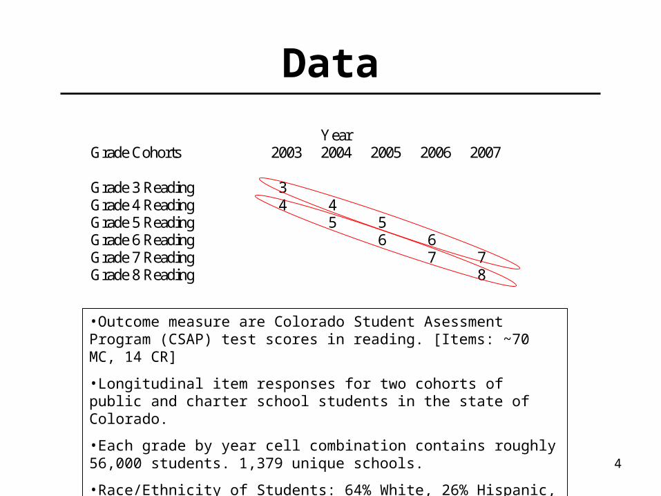
Year Grade Cohorts 2003 2004 2005 2006 2007 Grade 3 Reading 3 Grade 4 Reading 4 4 Grade 5 Reading 5 5 Grade 6 Reading 6 6 Grade 7 Reading 7 7 Grade 8 Reading 8

•Outcome measure are Colorado Student Asessment Program (CSAP) test scores in reading. [Items: ~70 MC, 14 CR]

•Longitudinal item responses for two cohorts of public and charter school students in the state of Colorado.

•Each grade by year cell combination contains roughly 56,000 students. 1,379 unique schools.

•Race/Ethnicity of Students: 64% White, 26% Hispanic, 6.3% Black

5

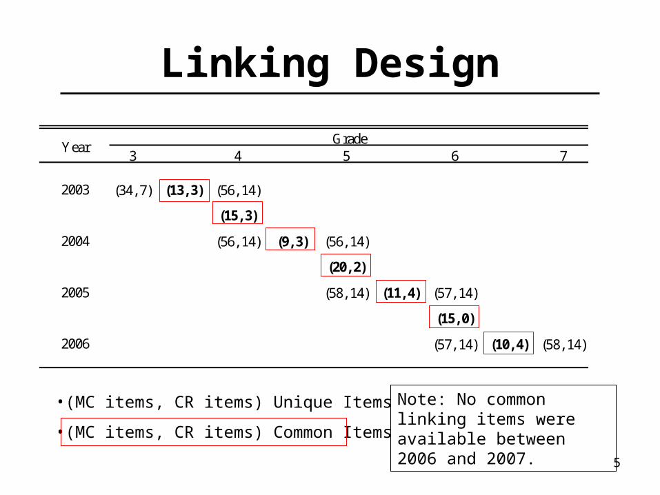
Linking Design

3 4 5 6 7

(34, 7) (13, 3) (56, 14)

(56, 14) (9, 3) (56, 14)

(58, 14) (11, 4) (57, 14)

(57, 14) (10, 4) (58, 14)

YearGrade

(15, 3)

(20, 2)

(15, 0)

2003

2004

2005

2006

•(MC items, CR items) Unique Items

•(MC items, CR items) Common Items

Note: No common linking items were available between 2006 and 2007.

6

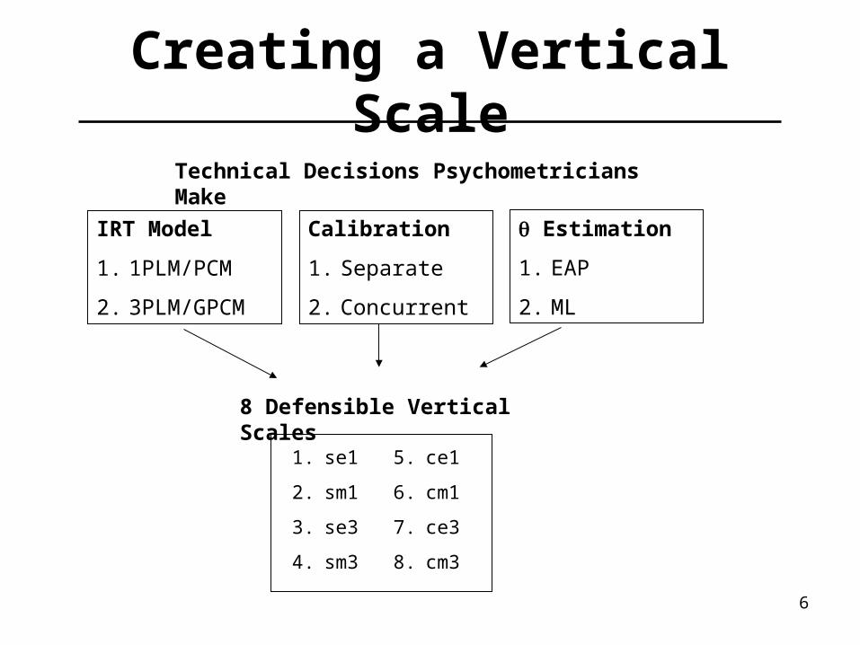
Creating a Vertical Scale

IRT Model

1. 1PLM/PCM

2. 3PLM/GPCM

Calibration

1. Separate

2. Concurrent

Estimation

1. EAP

2. ML

Technical Decisions Psychometricians Make

1. se1

2. sm1

3. se3

4. sm3

5. ce1

6. cm1

7. ce3

8. cm3

8 Defensible Vertical Scales

7

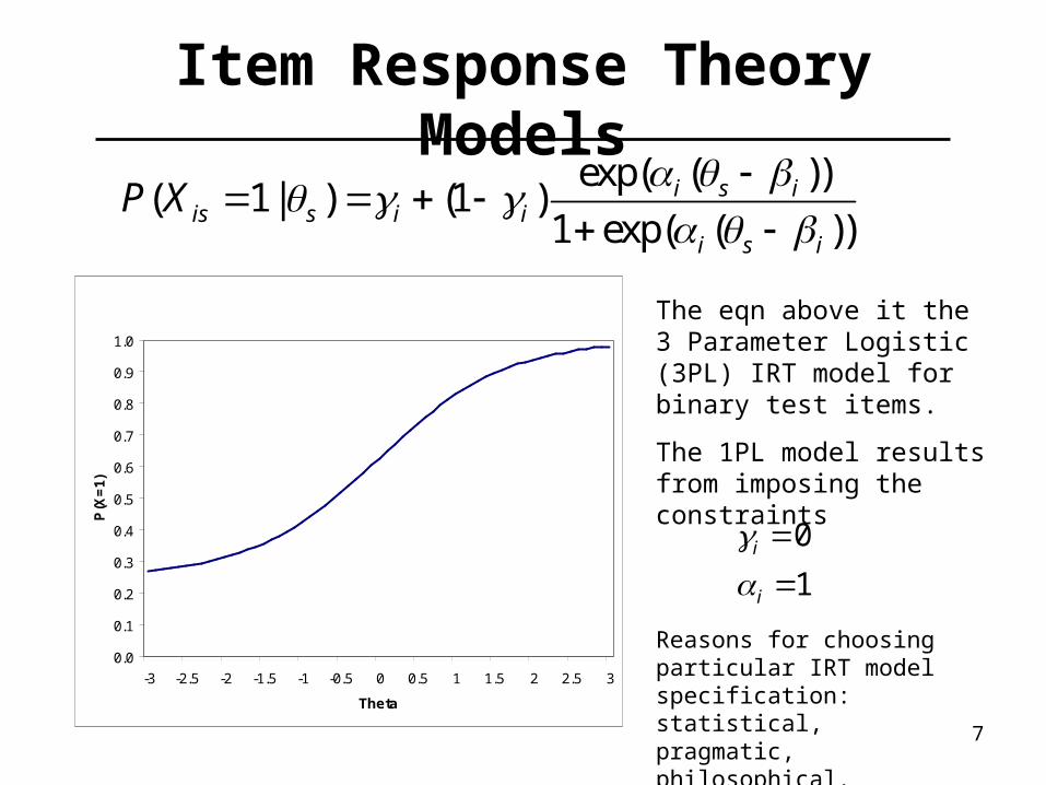
Item Response Theory Modelsexp( ( ))

( 1| ) (1 )1 exp( ( ))

i s iis s i i

i s i

P X

0.0

0.1

0.2

0.3

0.4

0.5

0.6

0.7

0.8

0.9

1.0

-3 -2.5 -2 -1.5 -1 -0.5 0 0.5 1 1.5 2 2.5 3

Theta

P(X

=1)

The eqn above it the 3 Parameter Logistic (3PL) IRT model for binary test items.

The 1PL model results from imposing the constraints

0

1i

i

Reasons for choosing particular IRT model specification: statistical, pragmatic, philosophical.

8

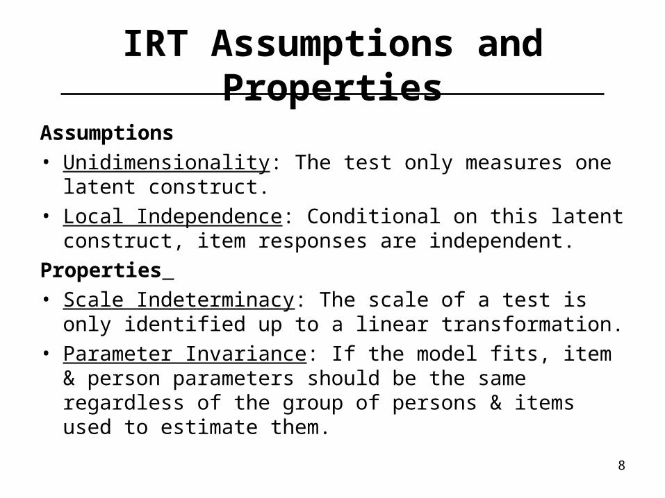
IRT Assumptions and Properties

Assumptions• Unidimensionality: The test only measures one latent

construct.• Local Independence: Conditional on this latent construct,

item responses are independent.

Properties • Scale Indeterminacy: The scale of a test is only identified

up to a linear transformation. • Parameter Invariance: If the model fits, item & person

parameters should be the same regardless of the group of persons & items used to estimate them.

9

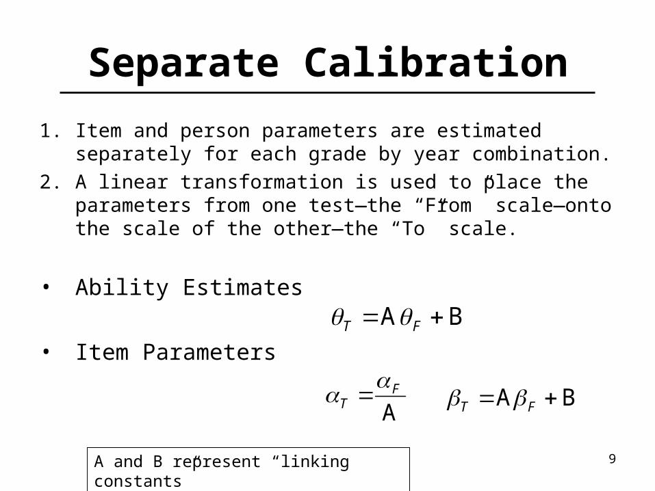
Separate Calibration

1. Item and person parameters are estimated separately for each grade by year combination.

2. A linear transformation is used to place the parameters from one test—the “From” scale—onto the scale of the other—the “To” scale.

• Ability Estimates

• Item Parameters

BA FT

AF

T

BA FT

A and B represent “linking constants”

10

-4 -2 0 2 4

0.0

0.2

0.4

0.6

0.8

1.0

Theta

Pro

ba

bili

ty

-4 -2 0 2 4

0.0

0.2

0.4

0.6

0.8

1.0

Theta

Pro

ba

bili

ty

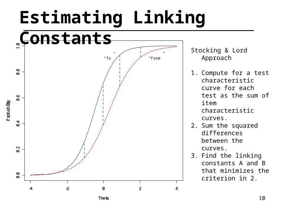
“To” “From”

Stocking & Lord Approach

1. Compute for a test characteristic curve for each test as the sum of item characteristic curves.

2. Sum the squared differences between the curves.

3. Find the linking constants A and B that minimizes the criterion in 2.

Estimating Linking Constants

11

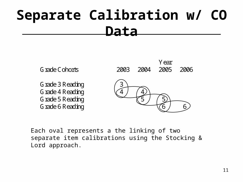
Separate Calibration w/ CO Data

Each oval represents a the linking of two separate item calibrations using the Stocking & Lord approach.

Year Grade Cohorts 2003 2004 2005 2006 Grade 3 Reading 3 Grade 4 Reading 4 4 Grade 5 Reading 5 5 Grade 6 Reading 6 6

12

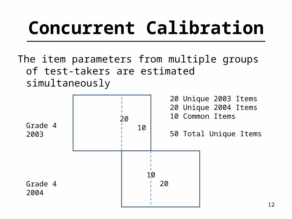
Concurrent Calibration

The item parameters from multiple groups of test-takers are estimated simultaneously

20 10

10 20

Grade 42003

Grade 42004

20 Unique 2003 Items20 Unique 2004 Items10 Common Items

50 Total Unique Items

13

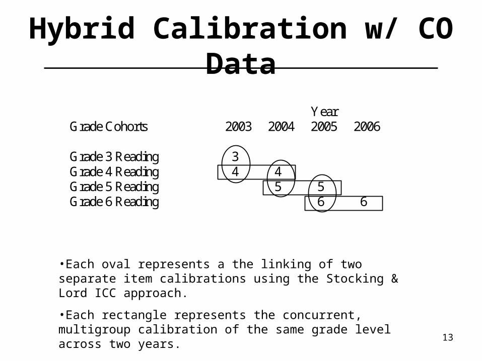
Hybrid Calibration w/ CO Data

•Each oval represents a the linking of two separate item calibrations using the Stocking & Lord ICC approach.

•Each rectangle represents the concurrent, multigroup calibration of the same grade level across two years.

Year Grade Cohorts 2003 2004 2005 2006 Grade 3 Reading 3 Grade 4 Reading 4 4 Grade 5 Reading 5 5 Grade 6 Reading 6 6

14

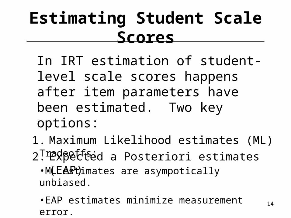
Estimating Student Scale Scores

In IRT estimation of student-level scale scores happens after item parameters have been estimated. Two key options:

1. Maximum Likelihood estimates (ML)

2. Expected a Posteriori estimates (EAP)

Tradeoffs:

•ML estimates are asympotically unbiased.

•EAP estimates minimize measurement error.

15

Value-Added Models

1. Parametric Growth (HLM)

2. Non-Parametric Growth (Layered Model)

16

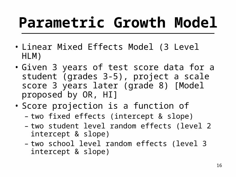
Parametric Growth Model

• Linear Mixed Effects Model (3 Level HLM)• Given 3 years of test score data for a student

(grades 3-5), project a scale score 3 years later (grade 8) [Model proposed by OR, HI]

• Score projection is a function of – two fixed effects (intercept & slope)– two student level random effects (level 2 intercept

& slope)– two school level random effects (level 3 intercept

& slope)

17

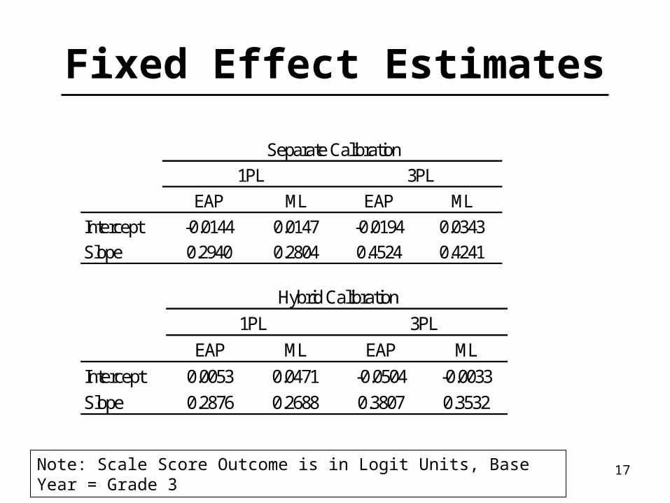
Fixed Effect Estimates

EAP ML EAP MLIntercept -0.0144 0.0147 -0.0194 0.0343Slope 0.2940 0.2804 0.4524 0.4241

Separate Calibration1PL 3PL

EAP ML EAP MLIntercept 0.0053 0.0471 -0.0504 -0.0033Slope 0.2876 0.2688 0.3807 0.3532

Hybrid Calibration1PL 3PL

Note: Scale Score Outcome is in Logit Units, Base Year = Grade 3

18

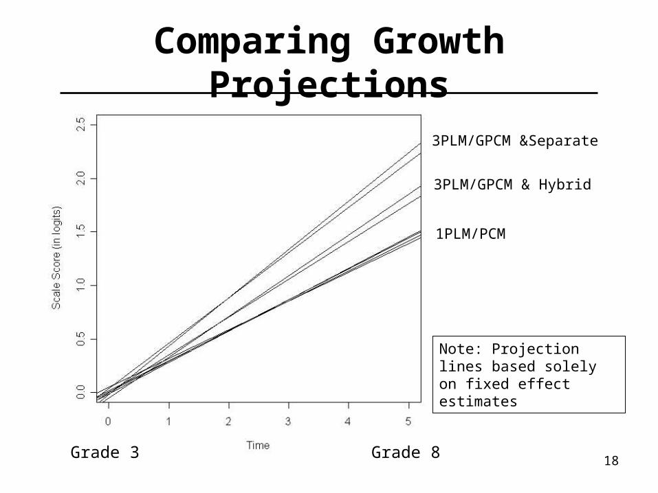
Comparing Growth Projections

1PLM/PCM

3PLM/GPCM & Hybrid

3PLM/GPCM &Separate

Grade 3 Grade 8

Note: Projection lines based solely on fixed effect estimates

19

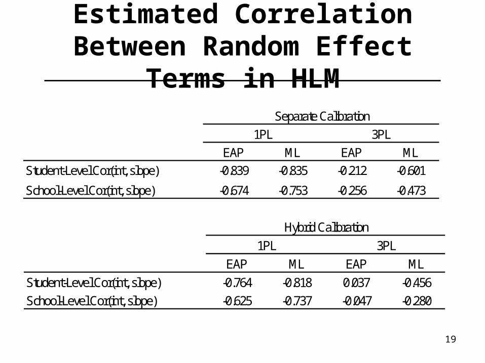
Estimated Correlation Between Random Effect Terms in HLM

EAP ML EAP MLStudent-Level Cor(int, slope) -0.839 -0.835 -0.212 -0.601

School-Level Cor(int, slope) -0.674 -0.753 -0.256 -0.473

1PL 3PLSeparate Calibration

EAP ML EAP MLStudent-Level Cor(int, slope) -0.764 -0.818 0.037 -0.456School-Level Cor(int, slope) -0.625 -0.737 -0.047 -0.280

1PL 3PLHybrid Calibration

20

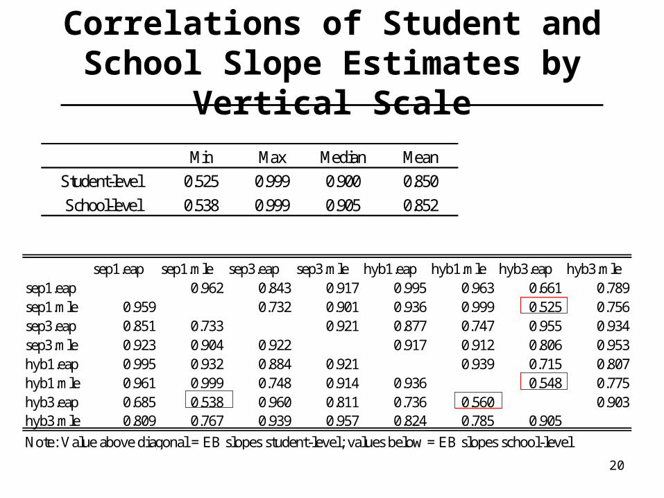
Correlations of Student and School Slope Estimates by Vertical Scale

sep1.eap sep1.mle sep3.eap sep3.mle hyb1.eap hyb1.mle hyb3.eap hyb3.mlesep1.eap 0.962 0.843 0.917 0.995 0.963 0.661 0.789sep1.mle 0.959 0.732 0.901 0.936 0.999 0.525 0.756sep3.eap 0.851 0.733 0.921 0.877 0.747 0.955 0.934sep3.mle 0.923 0.904 0.922 0.917 0.912 0.806 0.953hyb1.eap 0.995 0.932 0.884 0.921 0.939 0.715 0.807hyb1.mle 0.961 0.999 0.748 0.914 0.936 0.548 0.775hyb3.eap 0.685 0.538 0.960 0.811 0.736 0.560 0.903hyb3.mle 0.809 0.767 0.939 0.957 0.824 0.785 0.905

Note: Value above diagonal = EB slopes student-level; values below = EB slopes school-level

Min Max Median MeanStudent-level 0.525 0.999 0.900 0.850School-level 0.538 0.999 0.905 0.852

21

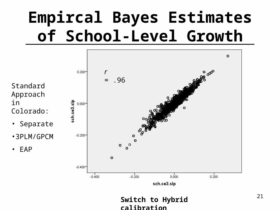
Empircal Bayes Estimates of School-Level Growth

Standard Approach in Colorado:

• Separate

•3PLM/GPCM

• EAP

Switch to Hybrid calibration

r = .96

22

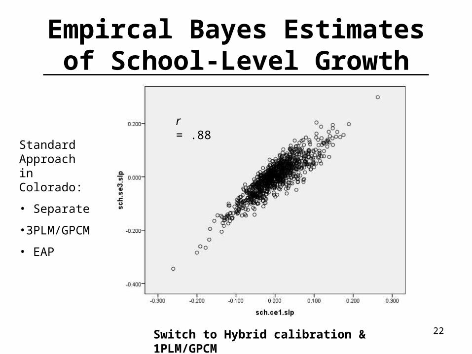
Empircal Bayes Estimates of School-Level Growth

Standard Approach in Colorado:

• Separate

•3PLM/GPCM

• EAP

Switch to Hybrid calibration & 1PLM/GPCM

r = .88

23

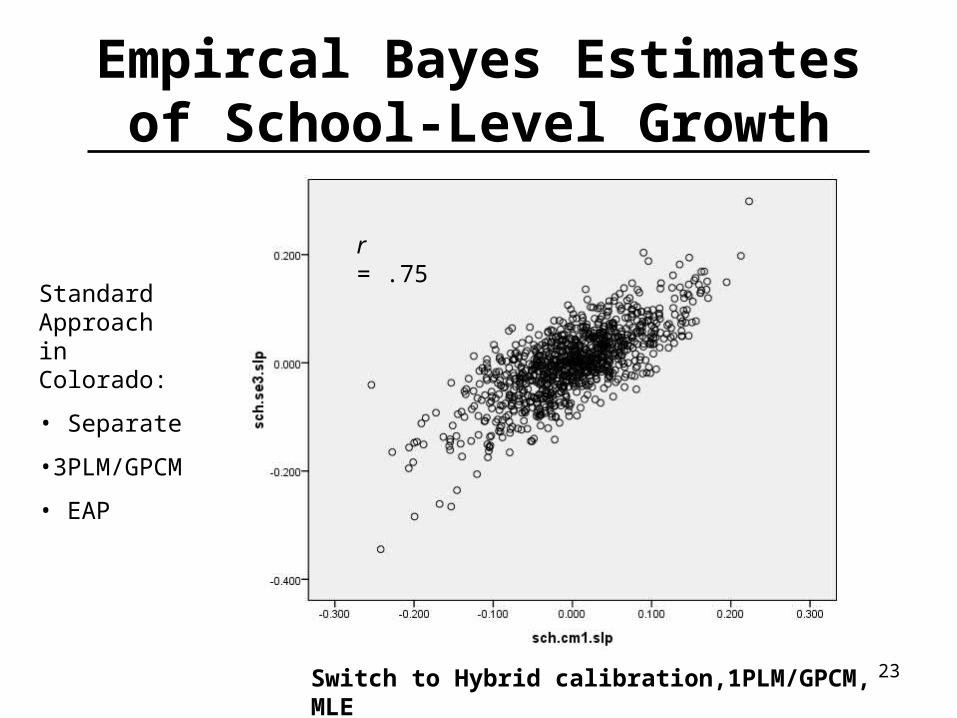
Empircal Bayes Estimates of School-Level Growth

Standard Approach in Colorado:

• Separate

•3PLM/GPCM

• EAP

Switch to Hybrid calibration,1PLM/GPCM, MLE

r = .75

24

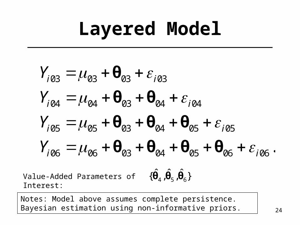
Layered Model

03 03 03 03

04 04 03 04 04

05 05 03 04 05 05

06 06 03 04 05 06 06.

i i

i i

i i

i i

Y

Y

Y

Y

θ

θ θ

θ θ θ

θ θ θ θ

Value-Added Parameters of Interest: 4 5 6ˆ ˆ ˆ{ , , }θ θ θ

Notes: Model above assumes complete persistence. Bayesian estimation using non-informative priors.

25

Differences in Schools Identified

Grade 4 Percent of Percent of Schools Identified (N=941)

0%

20%

40%

60%

80%

100%

1PL EAP 1PL MLE 3PL EAP 3PL MLE 1PL EAP 1PL MLE 3PL EAP 3PL MLE

Separate Hybrid

Below Average Average Above Average

26

Grade 5Grade 5 Percent of Percent of Schools Identified (N=950)

0%

20%

40%

60%

80%

100%

1PL EAP 1PL MLE 3PL EAP 3PL MLE 1PL EAP 1PL MLE 3PL EAP 3PL MLE

Separate Hybrid

Below Average Average Above Average

27

Grade 6Grade 6 Percent of Percent of Schools Identified (N=640)

0%

20%

40%

60%

80%

100%

1PL EAP 1PL MLE 3PL EAP 3PL MLE 1PL EAP 1PL MLE 3PL EAP 3PL MLE

Separate Hybrid

Below Average Average Above Average

28

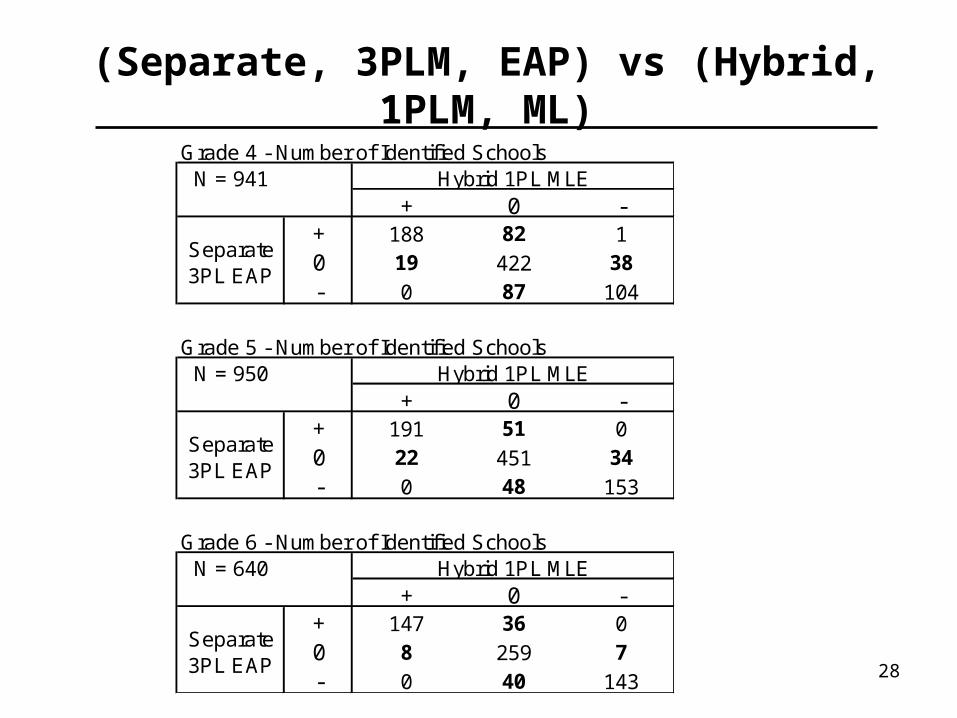
(Separate, 3PLM, EAP) vs (Hybrid, 1PLM, ML)G rade 4 - Number of Identified S chools

N = 941+ 0 -

+ 188 82 10 19 422 38- 0 87 104

G rade 5 - Number of Identified S choolsN = 950

+ 0 -+ 191 51 00 22 451 34- 0 48 153

G rade 6 - Number of Identified S choolsN = 640

+ 0 -+ 147 36 00 8 259 7- 0 40 143

S eparate 3P L E AP

Hybrid 1P L ML E

S eparate 3P L E AP

S eparate 3P L E AP

Hybrid 1P L ML E

Hybrid 1P L ML E

29

Conclusion

• Vertical scales have (largely) arbitrary metrics.• Absolute interpretations of parametric growth can

deceive.– Students might appear to grow “faster” solely because

of the scaling approach.– Can criterion-referencing (i.e., standard-setting)

reliably take this into account?• A better approach might focus on changes in norm-

referenced interpretations (but this conflicts with the NCLB perspective on growth).

• The layered model was less sensitive to the choice of scale, but there are still some noteworthy differences in numbers of schools identified.

30

Future Directions

• Full concurrent calibration.

• Running analysis with math tests.

• Joint analysis with math and reading tests.

• Acquiring full panel data.

• Developing a multidimensional vertical scale.

derek.briggs@colorado.edu