vidyalankarvidyalankar.org/file/bsc-it/sem_vi_classroom/dw_soln.pdfprelim question paper solution...

1

Vidyalankar T.Y. B.Sc. (IT) : Sem. VI Data Warehousing

Prelim Question Paper Solution

Data Warehouse Creating data to be analytical requires that it be subject-oriented, integrated, time-referenced, and non-volatile.

Subject-Oriented Data In a data warehouse environment, information used for analysis is organized around subjectsemployees, accounts, sales, products, and so on. This subject specific design helps in reducing the query response time by searching through very few records to get an answer to the user’s question.

Integrated Data Integrated data refers to de-duplicating information and merging it from many sources into one consistent location. When short listing your top 20 customers, you must know that “HAL” and “Hindustan Aeronautics Limited” are one and the same. There must be just one customer number for any form of HAL or Hindustan Aeronautics Limited, in your database.

Time-Referenced Data The most important and most scrutinized characteristic of the analytical data is its prior state of being. In order words, time-referenced data essentially refers to its time-valued characteristic. For example, the user may ask “What were the total sales of product ‘A’ for the past three years on New Year’s Day across region ‘Y’?” To answer this question, you need to know the sales figures of the product on New Year’s Day in all the branches for that particular region.

Non-Volatile Data Since the information in a data warehouse is heavily queried against time, it is extremely important to preserve it pertaining to each and every business event of the company. The non-volatility of data, characteristic of data warehouse, enables users to dig deep into history and arrive at specific business decisions based on facts. Framework Of The Data Warehouse One of the reasons that data warehousing has taken such a long time to develop is that it is actually a very comprehensive technology. In fact, it can be best represented as an enterprise-wide framework for managing informational data within the organization. In order to understand how all the components involved in a data warehousing strategy are related, it is essential to have a Data Warehouse Architecture. Data Warehouse Architecture A data Warehouse Architecture (DWA) is a way of representing the overall structure of data, communication, processing and presentation that exists for

1. (a)

1. (b)

Vidyalankar : T.Y. B.Sc. (IT) DW

2

end-user computing within the enterprise. The architecture is made up of number of interconnected parts: Source System Source data transport layer Data quality control and data profiling layer Metadata management layer Data integration layer Data processing layer End user reporting layer Source System Operational systems process data to support critical operational needs. In order to do this, operational databases have been historically created to provide an efficient processing structure for a relatively small number of well-defined business transactions. However, because of the limited focus of operational systems, the databases designed to support operational systems have difficulty accessing the data for other management or informational purposes. This difficulty is amplified by the fact that many operational systems are often 10-15 years old. This in turn means that the data access technology available to obtain operational data is itself dated.

Source Data Transport Layer The data transport layer of the DWA, largely constitutes data trafficking. It particularly represents the tools and processes involved in transporting data from the source systems to the enterprise warehouse system.

Fig. 1: Data Warehouse Architecture

Since the data volume is huge, the interfaces with the source system have to be robust and scalable enough to manage secured data transmission. Traditionally, ftp has been used extensively to do the data transmission. However, recent technological advances have enabled various other tools like NDM transmission and connectDirect.


3

Data Quality Control and Data Profiling Layer Often, data quality causes the most concern in any data warehousing solution, Incomplete and inaccurate data will jeopardize the success of the data warehouse. Data warehouses do not generate their own data; rather they rely on the input data from the various source systems. It is very essential to measure the quality of the source data and take corrective action even before the information is processed and loaded into the target warehouse. Metadata Management Layer In order to have a fully functional warehouse, it is necessary to have a variety of metadata available as also facts about the end-user views of data and information about the operational databases. Ideally, end-users should be able to access data from the warehouse (or from the operational databases) without having to know where it resides or the form in which it is stored. Data Integration Layer The data integration layer is involved in scheduling the various tasks that must be accomplished to integrate data acquired from various source systems. A lot of formatting and cleansing activities happen in this layer so that the data is consistent across the enterprise. This layer is heavily driven by off-the-shelf tools consists of high-level job control for the many processes (procedures) that must occur to keep the data ware house up-to-date. Data Processing Layer The warehouse (core) is where the dimensionally modeled data resides. In some cases, one can think of the warehouse simply as a transformed view of the operational data; but modeled for analytical purposes. End User Reporting Layer Success of a data warehouse implementation largely depends upon ease of access to valuable information. In that sense, the end user reporting layer is a very critical component. Based on the business needs, there can be several types of reporting architectures and data access layers. Since most of the reports and queries are analytical in nature, there has to be a tight integration between the warehouse dimensional model and the reporting architecture. Defining Dimensional Model In a star schema, if a dimension is complex and contains relationships such as hierarchies, it is compressed or flattened to a single dimension. Another version of star schema is a snowflake schema. In a snowflake schema complex dimensions are normalized. Here, dimensions maintain relationships with other levels of the same dimension. In figure 2 when representing the snowflake schema, ‘category’ and ‘brand’ are kept as separate but are related to ‘product’. The fact table contains one or several numeric attributes that measure business performance. Examples are unit sales, dollar sales, number of shipments, number of passengers and so on. Facts must be numeric, since the purpose of the data model is to enable users to query and understand business performance metrics by summarizing data.

1. (c)


4

Fig. 1: Star Schema Model

The dimension tables describe the facts. If the fact is number of products sold, then the dimensions supporting it may be time, location, product, customer, channel and promotions. Where time describes when the product was sold; location describes what store in which are sold the product; customer describes who bought the product; channel describes which mode (off the counter, internet shopping, and telemarketing) was used and promotion describes which promotional offer triggered this sale.

Fig. 2 : Snowflake Model


5

Granularity Of Facts The granularity of a fact is the level of detail at which it is recorded. If data is to be analyzed effectively, it must be all at the same level of granularity. As a general rule, data should be kept at the highest (most detailed) level of granularity. This is because you cannot change data to a higher level of detail than what you have decided to maintain. You can, however, always roll up (summarize) the data to create a table with a lower level of granularity (next lowest level of detail). Proper understanding of granularity is essential to understanding several of the topics to be discussed later. The more granular the data, the more you can do with it. Excessive granularity brings needless space consumption and increases complexity. You can always aggregate details; you cannot decompose aggregates. Granularity is not absolute or universal across industries. This has two implications. First, grains are not predetermined; second, what is granular to one business may be summarized for another. The two primary grains in analytical modeling are the transaction and the periodic snapshot. The transaction will serve most businesses like selling, direct marketing brokerage, and credit card. The periodic snapshot will serve periodic balance businesses, like insurance and banking. (This does not imply that insurance and banking would not benefit by also keeping the transaction). Granularity is determined by: Number of parts to a key Granularity of those parts Adding elements to an existing key always increases the granularity of the data; removing any part of an existing key decreases its granularity. Using customer sales to illustrate this, a key of customer ID and period ID is less granular than customer ID, product ID and period ID. Say, we need to keep vehicles produced as a measure for an auto manufacturer. A key of vehicle make, factory ID, engine size and data, is less granular than a key of vehicle make, factory ID, engine size, emission type and date. Granularity is also determined by the inherent cardinality of the entities participating in the primary key. Take organization, customer and order as examples. There are more orders than customers, and more customers than organizations. Data at the order level is more granular than data at the customer level, and data at the customer level is more granular than data at the organization level.

Configuring the listener The listener is the utility that runs constantly in the background on the database server, listening for client connection requests to the database and handling

1. (d)

2. (a)


6

them. It can be installed either before or after the creation of a database, but there is one option during the database creation that requires the listener to be configuredso we’ll configure it now, before we create the database. Run Net Configuration Assistant to configure the listener. It is available under the Oracle menu on the Windows Start menu as shown in the following image: The welcome screen will offer us four tasks that we can perform with this assistant. We’ll select the first one to configure the listener. The next screen will ask you what we want to do with the listener. The four options are as follows: Add Reconfigure Delete Rename Only the Add option will be available since we are installing Oracle for the first time. The remainder of the options will be grayed out and will be unavailable for selection. If they are not, then there is a listener already configured and we can proceed to the next sectionCreating the database. The next screen is the protocol selection screen. It will have TCP already selected for us, which is what most installations will require. This is the standard communications protocol in use on the Internet and in most local networks. Leave that selected and proceed to the next screen to select the port number to use. The default port number is 1521, which is standard for communicating with Oracle database and is the one most familiar to anyone who has ever worked with an Oracle database. So, change it only if you want to annoy the Oracle people in your organization who have all memorized the default Oracle port of 1521. That is the last step. It will ask us if we want to configure another listener. Since we only need one, we’ll answer “no” and finish out the screens by clicking on the Finish button back on the main screen. OWB components and architecture Now that we’ve installed the database and OWB client, let’s talk about the various components that have just been installed that are a part of the OWB and the architecture of OWB in the database. Then we’ll perform one final task that is required before using OWB to create our data warehouse. Oracle Warehosue Builder is composed on the client of the Design Center (including the Control Center Manager) and the Repository Browser. The server components are the Control Center Service, the Repository (including Workspaces), and the Target Schema. A diagram illustrating the various components and their interactions follows:

2. (b)


7

Fig. 1

The Design Center is the main client graphical interface for designing our data warehouse. This is where we will spend a good deal of time to define our sources and targets, and describe the extract, transform, and load (ETL) processes we use to load the target from the sources. The ETL procedures are what we will define to carry out the extraction of the data from our sources, any transformations needed on it and subsequent loading into the data warehouse. What we will create in the Design Center is a logical design only, not a physical implementation. This logical design will be stored behind the scenes in a Workspace in the Repository on the server. The user interacts with the Design Center, which stores all its work in a Repository Workspace.

We will use the Control Center Manager for managing the creation of that physical implementation by deploying the designs we've created into the Target Schema. The process of deployment is OWB's method for creating physical objects from the logical definitions created using the Design Center. We'll then use the Control Center Manager to execute the design by running the code associated with the ETL that we’ve designed. The Control Center Manager interacts behind the scenes with the Control Center Service, which runs on the server as shown in the previous image. The user directly interacts with the Control Center Manager and the Design Center only.

The Target Schema is where OWB will deploy the objects to, and where the execution of the ETL processes that load our data warehouse will take place. It is the actual data warehouse schema that gets built. It contains the objects that were designed in the Design Center, as well as the ETL code to load those objects. The Target Schema is not an actual Warehouse Builder software component, but is a part of the Oracle Database. However, it will contain Warehouse Builder components such as synonyms that will allow the ETL mappings to access objects in the Repository.

The Repository is the schema that hosts the design metadata definitions we create for our sources, targets, and ETL processes. Metadata is basically data about data. We will be defining sources, targets, and ETL processes using the Design Center and the information about what we have defined (the metadata) is stored in the repository.


8

Three Components of design center Before discussing the project in more detail, let's talk about the three windows in the main Design Center screen. They are as follows: • Project Explorer • Connection Explorer • Global Explorer The Project Explorer window is where we will work on the objects that we are going to design for our data warehouse. It has nodes for each of the design objects we'll be able to create. It is not necessary to make use of every one of them for every data warehouse we design, but the number of options available shows the flexibility of the tool. The objects we need will depend on what we have to work with in our particular situation. In our analysis earlier, we determined that we have to retrieve data from a database where it is stored. So, we will need to design an object under the Databases node to model that source database. If we expand the Databases node in the tree, we will notice that it includes both Oracle and Non-Oracle databases. We are not restricted to interacting with just Oracle in Warehouse Builder, which is one of its strengths. We will also talk about pulling data from a flat file, in which case we would define an object under the Files node. If our organization was running one of the applications listed under the Applications node (which includes Oracle E-Business Suite, PeopleSoft, Siebel, or SAP) and we wanted to pull data from it, we'd design an object under the Applications node. The Project Explorer isn't just for defining our source data, it also holds information about targets. Later on when we start defining our target data warehouse structure, we will revisit this topic to design our database to hold our data warehouse. So the Project Explorer defines both the sources of our data and the targets, but we also need to define how to connect to them. This is what the Connection Explorer is for. The Connection Explorer is where the connections are defined to our various objects in the Project Explorer. The workspace has to know how to connect to the various databases, files, and applications we may have defined in our Project Explorer. As we begin creating modules in the Project Explorer, it will ask for connection information and this information will be stored and be accessible from the Connection Explorer window. Connection information can also be created explicitly from within the Connection Explorer. There are some objects that are common to all projects in a workspace. The Global Explorer is used to manage these objects. It includes objects such as Public Transformations or Public Data Rules. A transformation is a function, procedure, or package defined in the database in Oracle's procedural SQL language called PL/SQL. Data rules are rules that can be implemented to enforce certain formats in our data. Creating a SQL Server database module Now that we have our module created for the Oracle database, let's create one for the SQL Server POS transactional database: ACME_POS. First, let's talk in

2. (c)

2. (d)


9

brief about the external database connections in Oracle. If we expand the Databases node in the Project Explorer, we'll see Oracle, Non-Oracle, and Transportable Modules. The Non-Oracle entry has a little plus sign next to it that indicates there are further subnodes under it, so let's expand that to see what they are. In the following image, a number of databases are listed, including the one that says just ODBC:

Fig. 1

The POS transactional database is a Microsoft SQL Server database and we’ll notice that it is one of the databases listed by name under the Non-Oracle databases. We might think this is where we’ve going to create our source module for this import, but no.

Oracle makes use of Oracle Heterogeneous Services to make connections to other databases. This is a feature that makes a non-Oracle database appear as a remote Oracle database server. There are two components to make this work—the heterogeneous service that comes by default with the Oracle database and a separate agent that runs independently of the database. The agent facilitates the communication with the external non-Oracle database. That agent can take one of these two forms: • A transparent gateway agent that is tailored specifically to the database

being accessed. • A generic connectivity agent that is included with the Oracle Database and

which can be used for any external database.


10

The transparent gateway agents must be purchased and installed separately from the Oracle Database, and then configured to support the communication with the external database. They are provided for heavy-duty applications that do a large amount of external communication with other databases. This is much more than we need for this application and as we have to pay extra for it, we are going to stick with the generic connectivity agent that comes free with the Oracle Database. It is a low-end solution that makes use of ODBC or OLE-DB drivers for accessing the external database. ODBC (Open Database Connectivity) is a standard interface for accessing database systems and is platform and database independent. OLE-DB (Object Linking and Embedding-Database) is a Microsoft-provided programming interface that extends the capability provided by ODBC to add support for other types of non-relational data stores that do not implement SQL such as spreadsheets. Designing the cube In the case of the ACME Toys and Gizmos Company, we have seen that the main measure the management is concerned about is daily sales. There are other numbers we could consider such as inventory numbers: How much of each item is on hand? However, the inventory is not directly related to daily sales and wouldn’t make sense here. We can model an inventory system in a data warehouse that would be separate from the sales portion. But for our purpose, we’re going to model the sales. Therefore, our main measure is going to be the dollar amount of sales for each item.

In this case, we have a source system—the POS Transactional system—that maintains the dollar amount of sales for each line item in each sales transaction that takes place. This can provide us the level of detail we will want to capture and maintain in our cube, since we can definitely capture sales for each product at each store for each day. We have found out that the POS Transactional system also maintains the count of the number of a particular item sold in the transaction. This is an additional measure we will consider storing in our cube also, since we can see that it is at the same grain as the total sales. The count of items would still pertain to that single transaction just like the sales amount, and can be captured for each product, store, and even date.

Our design is drawn out in a star schema configuration showing the cube, which is surrounded by the dimensions with the individual items of information (attributes) we’ll want to store for each. It looks like the following:

Fig. 1

3. (a)


11

OK, we now have a design for our data warehouse. It’s time to see how OWB can support us in entering that design and generating its physical implementation in the database. Creating a target user and module Create a target user There are a couple of ways we can go about creating our target user—create the user directly in the database and then add to OWB, or use OWB to physically create the user. If we have to create a new user, and if it's on the same database as our repository and workspaces, it's a good idea to use OWB to create the user, especially if we are not that familiar with the SQL command to create a user. However, if our target schema were to be in another database on another server, we would have to create the user there. It's a simple matter of adding that user to OWB as a target, which we'll see in a moment. Let's begin in the Design Center under the Global Explorer. There we said it was for various objects that pertained to the workspace as a whole.

One of those object types is a Users object that exists under the Security node as shown here:

Fig. 1

Right-click on the Users node and select New.. to launch the Create User dialog box. With this dialog box, we are creating a workspace user. We create a workspace user by selecting a database user that already exists or create a new one in the database. If we already had a target user created in the database, this is where we would select it. We're going to click on the Create DB User... button to create a new database user.

3. (b)


12

We need to enter the system username and password as we need a user with DBA privileges in the database to be able to create a database user. We then enter a username and password for our new user. As we like to keep things basic, we'll call our new user ACME_DWH, for the ACME data warehouse. We can also specify the default and temporary tablespace for our new user, which we'll leave at the defaults. The dialog will appear like the following when completely filled in: The new user will be created when you click on the OK button, and will appear in the righthand window of the Create User dialog already selected for us. Click on the OK button and the user will be registered with the workspace, and we’ll see the new username if we expand the User node under Security in the Global Explorer. We can continue with creating our target module now that we have a user defined in the database to map to. Creating a Time dimension with the Time Dimension Wizard 1. The first step of the wizard will ask us for a name for our Time dimension.

We're going to call it DATE_DIM. If we try to use just DATE, it will give us an error message because that is a reserved word in the Oracle Database; so it won't let us use it.

2. The next step will ask us what type of storage to use for our new dimension. 3. Now this brings us to step 3, which asks us to specify the data generation

information for our dimension. The Time Dimension Wizard will be automatically creating a mapping for us to populate our Time dimension and will use this information to load data into it. It asks us what year we want to start with, and then how many total years to include starting with that year. The numbers entered here will be determined by what range of dates we expect to load the data for, which will depend on how much historical data we will have available to us. We have checked with the DBAs for ACME Toys and Gizmos Company to get an idea of how many years' worth of data they have and have found out that there is data going back three years. Based on this information, we're going to set the start year to 2007 with the number of years set to three to bring us up to 2009.

4. This step is where we choose the hierarchy and levels for our Time dimension. We have to select one of the two hierarchies. We can use the Normal Hierarchy of day, month, quarter, and year; or we can choose the Week Hierarchy, which consists of two levels only—the day and the calendar week. Notice that if we choose the Week Hierarchy, we won't be able to view data by month, quarter, or year as these levels are not available to us. This is seen in the following image:

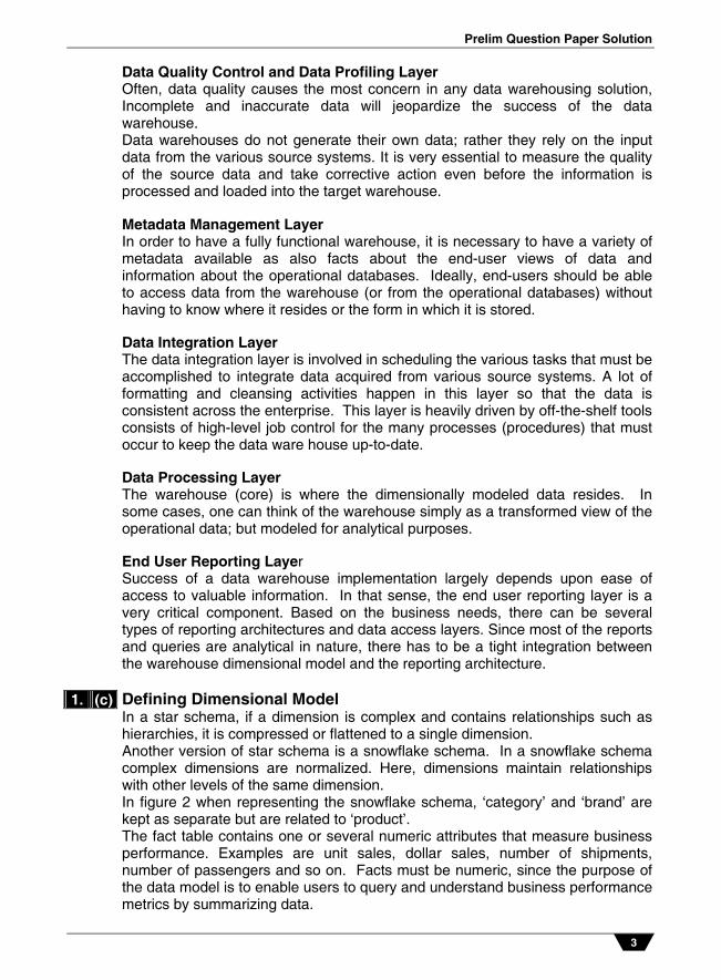
5. Let's move on to step 5 where the wizard will provide us the details about what it is going to create. An example is shown in the following image, which is what you should see if you've made all the same selections as we've moved along.

In the following image we can see the dimension attributes, levels, and

hierarchies that will be created:

3. (c)


13

Fig. 4

We can also see a couple of extra items at the bottom that we haven't discussed yet such as a sequence and a map name.

6. Continuing to the last step, it will display a progress bar as it performs each step and will display text in the main window indicating the step being performed. When it completes, we click on the Next button and it takes us to the final screen—the summary screen. This screen is a display of the objects it created and is similar to the previous display in step 5 of 6 that shows the pre-create settings. At this point, these objects have been created and we press the Finish button. Now we have a fully functional Time dimension for our data warehouse.

Creating a cube in OWB Creating a cube with the wizard We will start the wizard in a similar manner to how we started up the Dimension wizard. Right-click on the Cubes node under the ACME_DWH module in Project Explorer, select New, and then Using Wizard... to launch the cube-creation wizard. The first screen will be the welcome screen, which will summarize the steps.

3. (d)


14

The following are the steps in the creation process: 1. We proceed right to the first step where we give our cube a name. As we will

be primarily storing sales data, let's call our cube SALES and proceed to the next step.

2. In this step, we will select the storage type just as we did for the dimensions. We will select ROLAP for relational storage to match our dimension storage option, and then move to the next step.

3. In this step, we will choose the dimensions to include with our cube. We have defined three, and want all them all included. So, we can click on the double arrow in the center to move all the dimensions and select them. If we had more dimensions defined than we were going to include with this cube, we would click on each, and click on the single right arrow (to move each of them over); or we could select multiple dimensions at one time by holding down the Ctrl key as we clicked on each dimension. Then click the single right arrow to move those selected dimensions.

4. Moving on to the last step, we will enter the measures we would like the cube to contain. When we enter QUANTITY for the first measure and SALES_AMOUNT for the second one, we end up with a screen that should look similar to this with the dialog box expanded to show all the columns:

Clicking on Next in step 4 will bring us to the final screen where a summary of the actions it will take are listed. Selecting Finish on this screen will close the dialog box and place the cube in the Project Explorer.

The final screen looks like the following: Just as with the dimension wizard earlier, we get to see what the cube wizard

is going to create for us in the Warehouse Builder. We gave it a name, selected the dimensions to include, and specified the measures. The rest of the information was included by the wizard on its own. The wizard shows us that it will be creating a table named SALES for us that will contain the referenced columns, which it figured out from the dimension and measures information we provided. At this point, nothing has actually been created in the database apart from the definitions of the objects in the Warehouse Builder workspace. We can verify that if we look under the Tables entry under our ACME_DWH database node. We'll see a table named SALES along with tables named PRODUCT, STORE, and DATE_DIM. These are the tables corresponding to our three dimensions and the cube.

ETL The process of extracting, transforming, and loading data can appear rather complicated. We do have a special term to describe it, ETL, which contains the three steps mentioned. We're dealing with source data on different database systems from our target and a database from a vendor other than Oracle. Let's look from a high level at what is involved in getting that data from a source system to our target, and then take a look at whether to stage the data or not. We will then see how to automate that process in Warehouse Builder, which will relieve us of much of the work.

4. (a)


15

Manual ETL processes First of all, we need to be able to get data out of that source system and move it over to the target system. We can't begin to do anything until that is accomplished, but what means can we use to do so? We know that the Oracle Database provides various methods to load data into it. There is an application that Oracle provides called SQL*Loader, which is a utility to load data from flat files. This could be one way to get data from our source system. Every database vendor provides some means of extracting data from their tables and saving it to flat files. We could copy the file over and then use the SQL*Loader utility to load the file. Reading the documentation that describes how to use that utility, we see that we have to define a control file to describe the loading process and definitions of the fields to be loaded. This seems like a lot of work, so let's see what other options we might have. However, our target database structure doesn't look anything like the source database structure. The POS Transactional database is a relational database that is highly normalized, and our target consists of cubes and dimensions implemented relationally in the database. How are we going to get the data copied into that structure? Clearly, there will be some manipulation of the data to get it reformatted and restructured from source to target. We cannot just take all the rows from one table in the source structure and copy them into a table in the target structure for each source table. The data will have to be manipulated when it is copied. This means we need to develop code that can perform this rather complex task, depending on the manipulations that need to be done. In a nutshell, this is the process of extract, transform, and load. We have to: 1. Extract the data from the source system by some method. 2. Load flat files using SQL*Loader or via a direct database link. Then we have

to transform that data with SQL or PL/SQL code in the database to match and fit it into the target structure.

3. Finally, we have to load it into the target structure. The good news here is that the Warehouse Builder provides us the means to design this process graphically, and then generate all the code we need automatically so that we don’t have to build all that code manually. Mappings and operators in OWB Mapping: The Mapping window is the main working area on the right where

we will design the mapping. This window is also referred to as the canvas. The Data Object Editor used the canvas to lay out the data objects and connect them, whereas this editor lays out the mapping objects and connects them. This is the graphical display that will show the operators being used and the connections between the operators that indicate the data flow from source to target.

• Explorer: This window is similar to the Project Explorer window from the

Design Center, and is the same as the window in the Data Object Editor. It has the same two tabs—the Available Objects tab and the Selected Objects tab. It displays the same information that appears in the Project Explorer, and

4. (b)


16

allows us to drag and drop objects directly into our mapping. The tabs in this window are: Available Objects: This tab is almost like the Project Explorer. It

displays objects defined in our project elsewhere, and they can be dragged and dropped into this mapping.

Selected Objects: This tab displays all the objects currently defined in our mapping. When an object is selected in the canvas, the Selected Objects window will scroll to that object and highlight it. Likewise, if we select an object in the Selected Objects tab, the main canvas will scroll so that the object is visible and we will select it in the canvas. Go ahead and click on a few objects to see what the tab does.

Mapping properties: The mapping properties window displays the various

properties that can be set for objects in our mapping. It was called the Configuration window in Data Object Editor. When an object is selected in the canvas to the right, its properties will display in this window. It's hard to see in the previous image, but there is a window at the bottom of the properties window that will display an explanation for the property currently selected. We can resize any of these windows by holding the mouse pointer over the edge of a window until it turns into a double arrow, and then clicking and dragging to resize the window so we can see the contents better. To investigate the properties window a little closely, let's select the DATE_INPUTS operator. We can scroll the Explorer window until we see the operator and then click on it, or we can scroll the main canvas until we see it and then click on the top portion of the frame to select it. It is the first object on the left and defines inputs into DATE_DIM_MAP. It is visible in the previous image. After clicking on it, all the properties will be displayed in the mapping properties window. But wait a minute, nothing is displayed for this object; not every object has properties. Let's click on one of the attributes—YEAR_START_DATE—within the DATE_INPUTS operator. It can be selected in the Explorer or canvas and is shown in the following image, which is a portion of the Mapping Editor window we're referring to.

Now we can see some properties. YEAR_START_DATE is an attribute of the DATE_INPUTS object and defines the starting date to use for the data that will be loaded by this mapping. The properties that can be set or displayed for it include the characteristics about this attribute such as what kind of data type it is, its size, and its default value. Recalling our running of the Time Dimension Wizard there was one option to specify the year range for the dimension and we chose 2007 as the start year and that is what formed the source for the default value we can see here. Do not change anything but just click on a few more objects or attributes to look around at the various properties.

Palette: The Palette contains each of the objects that can be used in our

mapping. We can click on the object we want to place in the mapping and drag it onto the canvas. This list will be customized based on the type of editor we're using. The Mapping Editor will display mapping objects. The Data Object Editor will display data objects.


17

Bird's Eye View: This window displays a miniature version of the entire canvas and allows us to scroll around the canvas without using the scroll bars. We can click and drag the blue-colored box around this window to view various portions of the main canvas. The main canvas will scroll as we move the blue box. Go ahead and give that a try. We will find that in most mappings, we'll quickly outgrow the available space to display everything at once and will have to scroll around to see everything. This can come in very handy for rapidly scrolling the window.

Building the staging area table with the Data Object Editor To get started with building our staging area table, let's launch the OWB Design Center if it's not already running. Expand the ACME_DW_PROJECT node and let's take a look at where we're going to create this new table. We've stated previously that all the objects we design are created under modules in the Warehouse Builder so we need to pick a module to contain the new staging table. As we've decided to create it in the same database as our target structure, we already have a module created for this purpose. ACME_DWH, with a target module of the same name. The steps to create the staging area table in our target database are: 1. Navigate to the Databases | Oracle | ACME_DWH module. We will create

our staging table under the Tables node, so let's right-click on that node and select New... from the pop-up menu. Notice that there is no wizard available here for creating a table and so we are using the Data Object Editor to do it.

2. Upon selecting New..., we are presented with the Data Object Editor screen.

However, instead of looking at an object that's been created already, we're starting with a brand-new one. It will look similar to the following:

Fig. 4

3. The first tab is the Name tab where we'll give our new table a name. Let's call

it POS_TRANS_STAGE for Point-of-Sale transaction staging table. We'll just enter the name into the Name field, replacing the default TABLE_1 that it suggested for us.

4. (c)


18

4. Let's click on the Columns tab next and enter the information that describes the columns of our new table. We listed the key data elements that we will need for creating the columns. We didn't specify any properties of those data elements other than the name, so we'll need to figure that out.

5. We'll save our work using the Ctrl+S keys, or from the Diagram | Save All main menu entry in the Data Object Editor before continuing through the rest of the tabs. We didn't get to do this back in Chapter 2 when we first used the Data Object Editor.

The other tabs in Data Object Editor for a table are: • Constraints: The next tab after Columns is Constraints where we can enter

any one of the four different types of constraints on our new table. A constraint is a property that we can set to tell the database to enforce some kind of rule on the table that limits (or constrains) the values that can be stored in it. There are four types of constraints and they are:

Check constraint: a constraint on a particular column that indicates the acceptable values that can be stored in the column.

Foreign key: a constraint on a column that indicates a record must exist in the referenced table for the value stored in this column. A foreign key is also considered a constraint because it limits the values that can be stored in the column that is designated as a foreign key column.

Primary key: a constraint that indicates the column(s) that make up the unique information that identifies one and only one record in the table. It is similar to a unique key constraint in which values must be unique. The primary key differs from the unique key as other table's foreign key columns use the primary key value (or values) to reference this table. The value stored in the foreign key of a table is the value of the primary key of the referenced table for the record being referenced.

Unique key: a constraint that specifies the column(s) value combination(s) cannot be duplicated by any other row in the table.

• Indexes: The next tab provided in the Data Object Editor is the Indexes tab. An index can greatly facilitate rapid access to a particular record. It is generally useful for permanent tables that will be repeatedly accessed in a random manner by certain known columns of data in the table. It is not desirable to go through the effort of creating an index on a staging table, which will only be accessed for a short amount of time during a data load. Also, it is not really useful to create an index on a staging table that will be accessed sequentially to pull all the data rows at one time. An index is best used in situations where data is pulled randomly from large tables, but doesn't provide any benefit in speed if you have to pull every record of the table.

Partitions: So now that we have nixed the idea of creating indexes on our

staging table, let's move on to the next tab in the Data Object Editor for our table, Partitions. Partition is an advanced topic that we won't be covering here but for any real-world data warehouse, we should definitely consider implementing partitions. A partition is a way of breaking down the data stored in a table into subsets that are stored separately. This can greatly speed up


19

data access for retrieving random records, as the database will know the partition that contains the record being searched for based on the partitioning scheme used. It can directly home in on a particular partition to fetch the record by completely ignoring all the other partitions that it knows won't contain the record.

Attribute Sets: The next tab is the Attribute Sets tab. An Attribute Set is a

way to group attributes of an object in an order that we can specify when we create an attribute set. It is useful for grouping subsets of an object's attributes (or columns) for a later use. For instance, with data profiling (analyzing data quality for possible correction), we can specify attribute sets as candidate lists of attributes to use for profiling. This is a more advanced feature and as we won't need it for our implementation, we will not create any attribute sets.

Data Rules: The next tab is Data Rules. A data rule can be specified in the

Warehouse Builder to enforce rules for data values or relationships between tables. It is used for ensuring that only high-quality data is loaded into the warehouse. There is a seperate node—Data Rules—under our project in the Design Center that is strictly for specifying data rules. A data rule is created and stored under this node. This is a more advanced feature. We won't have time to cover it in this introductory book, so we will not have any data rules to specify here.

Data Viewer The last tab is the Data Viewer tab. This can be useful when

we've actually loaded data to this staging table to view it and verify that we got the results we expected.

This completes our tour through the tabs in the Data Object Editor for our table. These are the tabs that will be available when creating, viewing, or editing any table object. At this point, we've gone through all the tabs and specified any characteristics or attributes of our table that we needed to specify. This table object is now ready to use for mapping. Our staging area is now complete so we can proceed to creating a mapping to load it. We can now close the Data Object Editor window before proceeding by selecting Diagram | Close Window from the Data Object Editor menu.

Designing our mapping Now that we have our staging table defined, we are now ready to actually begin designing our mapping. We'll cover creating a mapping, adding/editing operators, and connecting operators together. Review of the Mapping Editor Mappings are stored in the Design Center under an Oracle Database module. In our case, we have created an Oracle Database module called ACME_DWH for our target database. So this is where we will create our mappings. In Design Center, navigate to the ACME_DW_PROJECT | Databases | Oracle | ACME_DWH | Mappings node if it is not already showing. Right-click on it and select New...from the resulting pop up. We will be presented with a dialog box to specify a name and, optionally, a description of our mapping. We'll name this mapping STAGE_MAP to reflect what it is being used for, and click on the OK button.

4. (d)


20

This will open the Mapping Editor for us to begin designing our mapping. An example of what we will see next is presented here:

Unlike our first look at the Mapping Editor in the last chapter where we looked at the existing DATE_DIM_MAP, all new mappings start out with a blank slate upon which we can begin to design our mapping. How we'd later see other editors similar to the Data Object Editor when looking at mappings, and that time has arrived now. By way of comparison with the Data Object Editor, the Mapping Editor has a blank area named Mapping where the Data Object Editor called it the Canvas. It basically performs the same function for viewing and laying out objects. The Mapping Editor has an Explorer window in common with the Data Object Editor. This window performs the same function for viewing operators/objects that can be dragged and dropped into our mapping, and the operators we've already defined in our mapping. Below the Explorer window in the Mapping Editor is the Properties window. In the Data Object Editor it was called Configuration. It is for viewing and/or editing properties of the selected element in the Mapping window. Right now we haven’t yet defined anything in our mapping, so it’s displaying our overall mapping properties. Below the Properties window is the Palette, which displays all the operators that can be dragged and dropped onto the Mapping window to design our mapping. It is just like the Palette in the Data Object Editor, but differs in the type of objects it displays. The objects in the case are specific to mappings, so we’ll see all the operators that are available to us. Store mapping Let's begin by creating a new mapping called STORE_MAP. We'll follow the procedure in the previous chapter to create a new mapping. In the Design Center, we will right-click on the Mappings node of the ACME_DW_PROJECT | Databases | Oracle | ACME_DWH database and select New.... Enter STORE_MAP for the name of the mapping and we will be presented with a blank Mapping Editor window. In this window, we will begin designing our mapping to load data into the STORE dimension. Adding source and target operators In the last chapter, we loaded data into the POS_TRANS_STAGE staging table with the intent to use that data to load our dimensions and cube. We'll now use this POS_TRANS_STAGE table as our source table. Let's drag this table onto the mapping from the Explorer window. Review the Adding source tables section of the previous chapter for a refresher if needed. The target for this mapping is going to be the STORE dimension, so we'll drag this dimension from Databases | Oracle | ACME_DWH | Dimensions onto the mapping and drop it to the right of the POS_TRANS_STAGE table operator. Remember that we build our mappings from the left to the right, with source on

5. (a)


21

the left and target on the right. We'll be sure to leave some space between the two because we'll be filling that in with some more operators as we proceed. Now that we have our source and target included, let's take a moment to consider the data elements we're going to need for our target and where to get them from the source. We might be tempted to include the ID fields in the above list of data elements for populating, but these are the attributes that will be filled in automatically by the Warehouse Builder. The Warehouse Builder fills them using the sequence that was automatically created for us when we built the dimension. We don't have to be concerned with connecting any source data to them. There is another attribute in our STORE dimension that we haven't accounted for yet—the COUNTY attribute. We don't have an input attribute to provide direct information about it. It is a special case that we will handle after we take care of these more straightforward attributes and will involve the lookup table that we discussed earlier in the introduction of this chapter. We're not going to directly connect the attributes mentioned in the list by just dragging a line between each of them. There are some issues with the source data that we are going to have to account for in our mapping. Connecting the attributes directly like that would mean the data would be loaded into the dimension as is, but we have investigated the source data and discovered that much of the source data contains trailing blanks due to the way the transactional system stores it. Some of the fields should be made all uppercase for consistency.

Given this additional information, we'll summarize the issues with each of the fields that need to be corrected before loading into the target and then we'll see how to implement the necessary transformations in the mapping to correct them:

STORE_NAME, STORE_NUMBER: We need to trim spaces and change these attributes to uppercase to facilitate queries as they are part of the business identifier

STORE_ADDRESS1, ADDRESS2, CITY, STATE, and ZIP_POSTALCODE: We need to trim spaces and change the STATE attribute to uppercase

STORE_REGION: We need to trim spaces and change this attribute to uppercase

All of these needs can be satisfied and we can have the desired effect by applying pre-existing SQL functions to the data via Transformation Operators. Product mapping The mapping for the PRODUCT dimension will be similar to the STORE mapping, so we won't cover it in as much detail here. We'll open the Design Center if it's not already open and create a new mapping just as we did for the STORE mapping earlier and the STAGE_MAP mapping from the last chapter. We'll name this mapping PRODUCT_MAP.

5. (b)


22

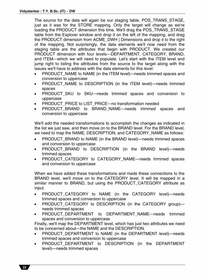
The source for the data will again be our staging table, POS_TRANS_STAGE, just as it was for the STORE mapping. Only the target will change as we're loading the PRODUCT dimension this time. We'll drag the POS_TRANS_STAGE table from the Explorer window and drop it on the left of the mapping, and drag the PRODUCT dimension from ACME_DWH | Dimensions and drop it to the right of the mapping. Not surprisingly, the data elements we'll now need from the staging table are the attributes that begin with PRODUCT. We created our PRODUCT dimension with four levels—DEPARTMENT, CATEGORY, BRAND, and ITEM—which we will need to populate. Let's start with the ITEM level and jump right to listing the attributes from the source to the target along with the issues we'll have to address with the data elements for this level: PRODUCT_NAME to NAME (in the ITEM level)—needs trimmed spaces and

conversion to uppercase PRODUCT_NAME to DESCRIPTION (in the ITEM level)—needs trimmed

spaces PRODUCT_SKU to SKU—needs trimmed spaces and conversion to

uppercase PRODUCT_PRICE to LIST_PRICE—no transformation needed PRODUCT_BRAND to BRAND_NAME—needs trimmed spaces and

conversion to uppercase We'll add the needed transformations to accomplish the changes as indicated in the list we just saw, and then move on to the BRAND level. For the BRAND level, we need to map the NAME, DESCRIPTION, and CATEGORY_NAME as follows:

PRODUCT_BRAND to NAME (in the BRAND level)—needs trimmed spaces and conversion to uppercase

PRODUCT_BRAND to DESCRIPTION (in the BRAND level)—needs trimmed spaces

PRODUCT_CATEGORY to CATEGORY_NAME—needs trimmed spaces and conversion to uppercase

When we have added these transformations and made these connections to the BRAND level, we'll move on to the CATEGORY level. It will be mapped in a similar manner to BRAND, but using the PRODUCT_CATEGORY attribute as input.

PRODUCT_CATEGORY to NAME (in the CATEGORY level)—needs trimmed spaces and conversion to uppercase

PRODUCT_CATEGORY to DESCRIPTION (in the CATEGORY group)—needs trimmed spaces

PRODUCT_DEPARTMENT to DEPARTMENT_NAME—needs trimmed spaces and conversion to uppercase

Finally, we'll map the DEPARTMENT level, which has just two attributes we need to be concerned about—the NAME and the DESCRIPTION. PRODUCT_DEPARTMENT to NAME (in the DEPARTMENT level)—needs

trimmed spaces and conversion to uppercase PRODUCT_DEPARTMENT to DESCRIPTION (in the DEPARTMENT

level)—needs trimmed spaces


23

When we have completed these additional connections and transformations, we will have completed the mapping for the PRODUCT dimension. It should look similar to the following screenshot, which shows all the transformations and connections in place that were described earlier:

Fig. 1

We have completed the mapping for our PRODUCT dimension, and that completes all the mappings for our dimensions we will need to do. There is a third dimension we'll be using, the DATE_DIM mapping, but that mapping was created automatically for us. Let's save our work with the Ctrl+S key combination, or with Design | Save All from the Design Center main menu, or with Mapping | Save All from the Mapping Editor main menu. Moving on, we'll now create a mapping to populate our cube and that will be all the mappings we'll need for our data warehouse. Validating We briefly touched upon the topic of validation of mapping when we were working on our SALES cube mapping and talked about the error we would get if we tried to map a date attribute to a number attribute. Error checking is what validation is for. The process of validation is all about making sure the objects and mappings we’ve defined in the Warehouse Builder have no obvious errors in design. Let’s recap how we go about performing a validation on an object we’ve created in the Warehouse Builder. There are a number of places we can perform a validation. One of them is the main Design Center. Validating in the Design Center There is a context menu associated with everything we create. You can access it on any object in the Design Center by right-clicking on the object of your choice. Let’s take a look at this by launching our Design Center, connecting as our ACMEOWB user, and then expanding our ACME_DW_PROJECT. Let’s find our staging table, POS_TRANS_STAGE, and use it to illustrate the validation of an

5. (c)


24

object from the Design Center. As we can recall, this table is under the ACME_DWH module in Oracle node and right-clicking on it will present. The validation will result in one of the following three possibilities: 1. The validation completes successfully with no warnings and/or errors as this

one did. 2. The validation completes successfully, but with some non-fatal warnings. 3. The validation fails due to one or more errors having been found. In any of these cases, we can look at the full message by double-clicking on the Message column in the window on the right. This will launch a small dialog box that contains the full text of the message. Validating from the editors The Data Object Editor and the Mapping Editor both provide for validation from within the editor. We'll talk about the Data Object Editor first and then about the Mapping Editor because there are some subtle differences. Validating in the Data Object Editor Let's double-click on the POS_TRANS_STAGE table name in the Design Center to launch the Data Object Editor so that we can discuss validation in the editor. We can right-click on the object displayed on the Canvas and select Validate from the pop-up menu, or we can select Validate from the Object menu on the main editor menu bar. Another option is available if we want to validate every object currently loaded into our Data Object Editor. It is to select Validate All from the Diagram menu entry on the main editor menu bar. We can also press the validate icon on the General toolbar, which is circled in the following image of the toolbar icons:

Fig. 3

Validating in the Mapping Editor We'll now load our STORE_MAP mapping into the Mapping Editor and take a look at the validation options in that editor. Unlike the Data Object Editor, validation in the Mapping Editor involves all the objects appearing on the canvas together because that is what composes the mapping. We can only view one mapping at a time in the editor. The Data Object Editor lets us view a number of separate objects at the same time. For this reason, we won't find a menu entry that says "Validate All" in the Mapping Editor. What we will find in the main editor menu bar's Mapping menu is an entry called Validate that we can select to validate this mapping. To the right of the Validate menu entry we can see the F4 key listed, which means we can validate our mapping by pressing the F4 key also. The key press we can do to validate is not


25

available in the Data Object Editor because it wouldn't know which object we intend to validate. We also have a toolbar in the Mapping Editor that contains an icon for validation, like the one we have in the Data Object Editor. It is the same icon as shown in the previous image of the Data Object Editor toolbar. Let's press the F4 key or select Validate from the Mapping menu or press the Validate icon in the toolbar. The same behavior will occur as in the Data Object Editor—the validation results will appear in the Generation Results window. The Control Center Manager window overview The Object Details window Let's click on the ACME_DWH_LOCATION again in the left window and look at the complete list of objects for our project. The statuses will vary depending on whether we've done any deployments or not, when we did them, and whether there are any warnings or failures due to errors that occurred. If you're following along exactly with the book, the only deployment we've done so far is the POS_TRANS_STAGE table and the previous image of the complete Control Center manager interface shows it as the only one that has been deployed successfully. The remainder all have a deploy status of Not Deployed. The columns displayed in the Object Details window are as follows: Object: The name of the object Design Status: The status of the design of the object in relation to whether it

has been deployed yet or not New: The object has been created in the Design Center, but has not

been deployed yet Unchanged: The Object has been created in the Design Center and

deployed previously, and has not been changed since its last deployment

Changed: The Object has been created and deployed, and has subsequently undergone changes in the Design Center since its last deployment subsequently undergone changes in the Design Center since its last deployment.

Deploy Action: What action will be taken upon the next deployment of this object in the Control Center Manager Create: Create the object; if an object with the same name already

exists, this can generate an error upon deployment Upgrade: Upgrade the object in place, preserving data Drop: Delete the object Replace: Delete and recreate the object; this option does not preserve

data Deployed: Date and time of the last deployment Deploy Status: Results of the last deployment

Not Deployed: The object has not been deployed yet Success: The last deployment was successful, without any errors or

warnings Warning: The last deployment had warnings Failed: The last deployment failed due to errors

5. (d)


26

Location: The location defined for the object, which is where it will be deployed

Module: The module where the object is defined. Some of the previous columns will allow us to perform an action associated

with the column by double-clicking or single-clicking in the column. The following is a list of the columns that have actions available, and how to access them:

Object: Double-click on the object name to launch the appropriate editor on the object.

Deploy Action: Click on the deploy action to change the deploy action for the next deployment of the object via a drop-down menu. The list of available actions that can be taken will be displayed. Not all the previously listed actions are available for every object. For instance, upgrade is not available for some objects and will not be an option for a mapping.

The Control Center Jobs window Every time we do a deployment or execute a mapping, a job is created by the Control Center to perform the action. The job is run in the background while we can continue working on other things, and the status of the job is displayed in the Control Center Jobs window. Looking back at the previous image of the Control Center manager, we can see the status of the POS_TRANS_STAGE table deployment that we performed. The green check mark indicates it was successful. If we want to see more details, especially if there were warnings or errors, we can double-click on the line in the Control Center Jobs window and it will pop up a dialog box displaying the details. An example of the dialog box is shown next:

Fig. 3

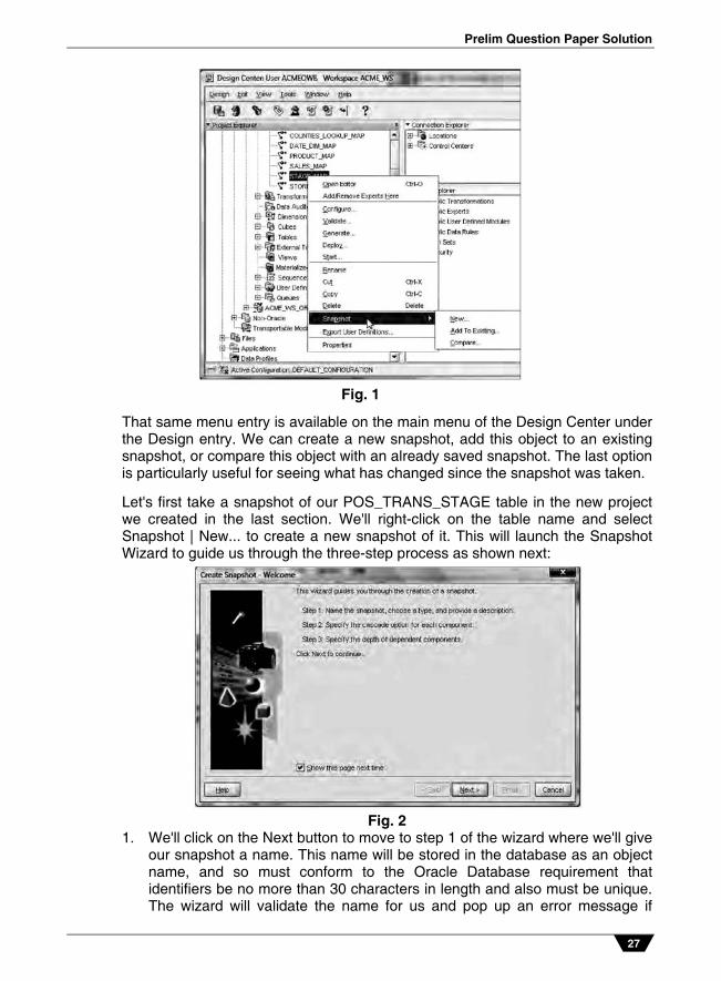
Snapshots A snapshot captures all the metadata information about an object at the time the snapshot is taken and stores it for later retrieval. It is a way to save a version of an object should we need to go back to a previous version or compare a current version with a previous one. We take a snapshot of an object from the Design Center by right-clicking on the object and selecting the Snapshot menu entry. This will give us three options to choose from as shown next:

6. (a)


27

Fig. 1

That same menu entry is available on the main menu of the Design Center under the Design entry. We can create a new snapshot, add this object to an existing snapshot, or compare this object with an already saved snapshot. The last option is particularly useful for seeing what has changed since the snapshot was taken.

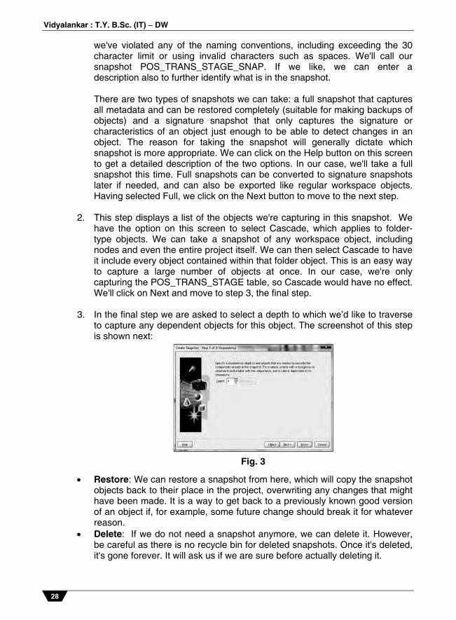
Let's first take a snapshot of our POS_TRANS_STAGE table in the new project we created in the last section. We'll right-click on the table name and select Snapshot | New... to create a new snapshot of it. This will launch the Snapshot Wizard to guide us through the three-step process as shown next:

Fig. 2

1. We'll click on the Next button to move to step 1 of the wizard where we'll give our snapshot a name. This name will be stored in the database as an object name, and so must conform to the Oracle Database requirement that identifiers be no more than 30 characters in length and also must be unique. The wizard will validate the name for us and pop up an error message if


28

we've violated any of the naming conventions, including exceeding the 30 character limit or using invalid characters such as spaces. We'll call our snapshot POS_TRANS_STAGE_SNAP. If we like, we can enter a description also to further identify what is in the snapshot.

There are two types of snapshots we can take: a full snapshot that captures all metadata and can be restored completely (suitable for making backups of objects) and a signature snapshot that only captures the signature or characteristics of an object just enough to be able to detect changes in an object. The reason for taking the snapshot will generally dictate which snapshot is more appropriate. We can click on the Help button on this screen to get a detailed description of the two options. In our case, we'll take a full snapshot this time. Full snapshots can be converted to signature snapshots later if needed, and can also be exported like regular workspace objects. Having selected Full, we click on the Next button to move to the next step.

2. This step displays a list of the objects we're capturing in this snapshot. We have the option on this screen to select Cascade, which applies to folder-type objects. We can take a snapshot of any workspace object, including nodes and even the entire project itself. We can then select Cascade to have it include every object contained within that folder object. This is an easy way to capture a large number of objects at once. In our case, we're only capturing the POS_TRANS_STAGE table, so Cascade would have no effect. We'll click on Next and move to step 3, the final step.

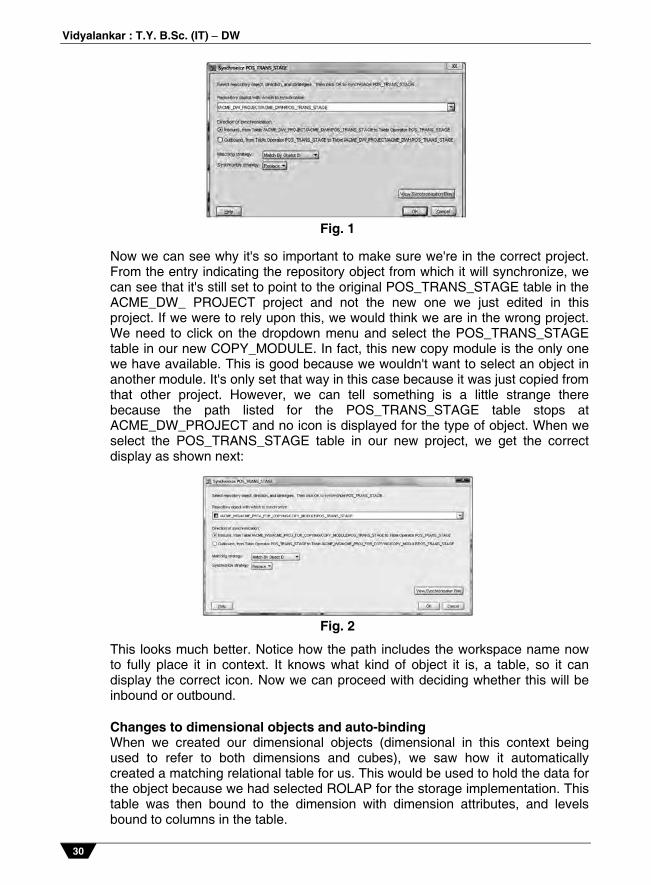
3. In the final step we are asked to select a depth to which we’d like to traverse

to capture any dependent objects for this object. The screenshot of this step is shown next:

Fig. 3

Restore: We can restore a snapshot from here, which will copy the snapshot objects back to their place in the project, overwriting any changes that might have been made. It is a way to get back to a previously known good version of an object if, for example, some future change should break it for whatever reason.

Delete: If we do not need a snapshot anymore, we can delete it. However, be careful as there is no recycle bin for deleted snapshots. Once it's deleted, it's gone forever. It will ask us if we are sure before actually deleting it.


29

Convert to Signature: This option will convert a full snapshot to a signature snapshot.

Export: We can export full snapshots like we can export regular workspace objects. This will save the metadata in a file on disk for backup or for importing later.

• Compare: This option will let us compare two snapshots to each other to see what the differences are.

Synchronizing Many operators we use in a mapping represent a corresponding workspace object. If the workspace object (for instance, a table) changes, then the operator also needs to change to be kept in sync. The process of synchronization is what accomplishes that, and it has to be invoked by us when changes are made.

Now that we have the updated table definition for the POS_TRANS_STAGE table, we have to turn our attention to any mappings that have included a table operator for the changed table because they will have to be synchronized to pick up the change. These operators are bound to an actual table using a table definition like we just edited. When the underlying table definition gets updated, we have to synchronize those changes with any mappings that include that table. We now have our STAGE_MAP mapping copied over to our new project. So let's open that in the mapping editor by double-clicking on it and investigate the process of synchronizing. When we open the mapping for the first time, it may have all the objects overlapping in the middle of the mapping. So we'll just click on the auto-layout button, If we look at the POS_TRANS_STAGE mapping operator, we can scroll down the INOUTGRP1 attribute group or maximize the operator to view all the attributes to see that the new STORE_AREA_SIZE column is not included. To update the operator in the mapping to include the new column name, we must perform the task of synchronization, which reconciles the two and makes any changes to the operator to reflect the underlying table definition. We could just manually edit the properties for the operator to add the new column name, but that still wouldn't actually synchronize it with the actual table. Doing the synchronization will accomplish both—add the new column name and synchronize with the table. In this particular case there is another reason to synchronize, and that is we copied this mapping into the new project from another mapping where it was already synchronized with tables in that project. This synchronization information is not automatically updated when the mapping is copied. To synchronize, we right-click on the header of the table operator in the mapping and select Synchronize... from the pop-up menu, or click on the table operator header and select Synchronize... from the main menu Edit entry, or press the F7 key. This will pop up the Synchronize dialog box as shown next:

6. (b)


30

Fig. 1

Now we can see why it's so important to make sure we're in the correct project. From the entry indicating the repository object from which it will synchronize, we can see that it's still set to point to the original POS_TRANS_STAGE table in the ACME_DW_ PROJECT project and not the new one we just edited in this project. If we were to rely upon this, we would think we are in the wrong project. We need to click on the dropdown menu and select the POS_TRANS_STAGE table in our new COPY_MODULE. In fact, this new copy module is the only one we have available. This is good because we wouldn't want to select an object in another module. It's only set that way in this case because it was just copied from that other project. However, we can tell something is a little strange there because the path listed for the POS_TRANS_STAGE table stops at ACME_DW_PROJECT and no icon is displayed for the type of object. When we select the POS_TRANS_STAGE table in our new project, we get the correct display as shown next:

Fig. 2

This looks much better. Notice how the path includes the workspace name now to fully place it in context. It knows what kind of object it is, a table, so it can display the correct icon. Now we can proceed with deciding whether this will be inbound or outbound. Changes to dimensional objects and auto-binding When we created our dimensional objects (dimensional in this context being used to refer to both dimensions and cubes), we saw how it automatically created a matching relational table for us. This would be used to hold the data for the object because we had selected ROLAP for the storage implementation. This table was then bound to the dimension with dimension attributes, and levels bound to columns in the table.


31

Single Hypercube vs. Multicube Just as in a relational database, where the data is typically stored in a series of two dimensional tables, the data in an OLAP database consists of values with differing dimensionality. For example, consider the case of a bank which wants to analyze profitability by customer and product. Certain revenues may be dimensioned by customer, product, time, geography and scenario. But costs such as back office salaries might be dimensioned by cost type, cost center and time. Thus, a real world multidimensional database must be capable of storing data that has differing dimensionality in a single logical database that presents a single conceptual view to the user.

It is not acceptable to insist that all data in the model be dimensioned by the same criteria. Putting data into an element called “no product” because the data item happens not to be dimensioned by product, merely serves to confuse the user. Products that cannot support a multicube architecture with the ability to logically relate cubes, force unreasonable compromises on the developer of sophisticated models. Not only does it make the access to the data less logical but it can have serious adverse effects on database size and retrieval efficiency. Data Sparsity And Data Explosion The reality of data explosion in multidimensional databases is a surprising and widely misunderstood phenomenon. For those about to implement a project with considerable exposure to OLAP products, it is critically important to understand what data sparsity and data explosion are, what causes these, and how these can be avoided for, the consequences of ignoring data explosion can be very costly and, in most cases, result in project failure. Input data or base data (i.e. before calculated hierarchies or levels) in OLAP applications is typically sparse (not densely populated). Also, as the number of dimensions increase, data will typically become sparser (less dense).

For example, in a one-dimensional matrix, you can suppress all zero values and, therefore, have a 100 percent dense matrix. In a two dimensional matrix, you cannot suppress zeros if there is a non-zero value in any element in the two dimensions (see figure 1 and 2). While it is not true in all cases, typically, as the number of dimensions in a model increases, so does the data sparsity. For example, if you are storing sales data by product and by month, it is conceivable that you will sell each product each month (100 percent dense).

Fig. 1: 100 Per cent Dense Structure

However, if you were storing sales data, by product, by customer, by region, by month, clearly you would not sell each product to every customer in every region every month.

6. (c)

6. (d)


32

Fig. 2 : 25 Per cent Dense Structure4 out of 16 data Points Populated

By adding the dimension “gender” to this model, you would double the possible size of the cube by storing the data by either of the two variables male or female, but the size of the stored data would remain the same. In this case, by introducing another simple dimension, the sparsity will have doubled!

Data explosion is the phenomenon that occurs in multidimensional models where the derived or calculated values significantly exceed the base values. There are three main factors that contribute to data explosion. 1. Sparsely populated base data increases the likelihood of data explosion. 2. Many dimensions in a model increase the likelihood of data explosion, and 3. A high number of calculated levels in each dimension increase the likelihood

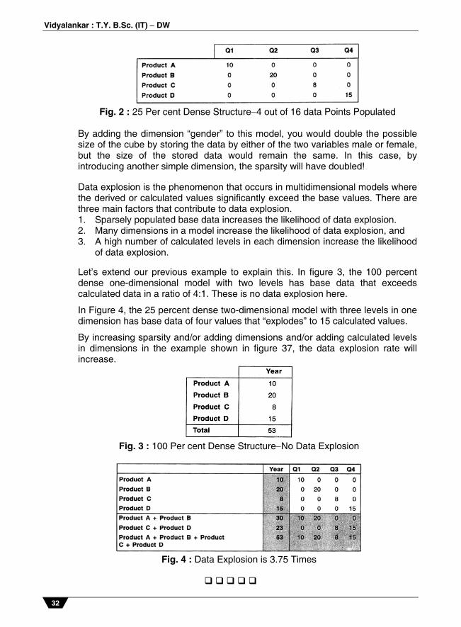
of data explosion. Let’s extend our previous example to explain this. In figure 3, the 100 percent dense one-dimensional model with two levels has base data that exceeds calculated data in a ratio of 4:1. These is no data explosion here.

In Figure 4, the 25 percent dense two-dimensional model with three levels in one dimension has base data of four values that “explodes” to 15 calculated values.

By increasing sparsity and/or adding dimensions and/or adding calculated levels in dimensions in the example shown in figure 37, the data explosion rate will increase.

Fig. 3 : 100 Per cent Dense StructureNo Data Explosion

Fig. 4 : Data Explosion is 3.75 Times

vidyalankarvidyalankar.org/file/bsc-it/sem_vi_classroom/dw_soln.pdfprelim question paper solution...

Documents