viability study of a residential integrated stormwater

University of Central Florida University of Central Florida

STARS STARS

Electronic Theses and Dissertations, 2004-2019

2011

Viability Study Of A Residential Integrated Stormwater, Graywater, Viability Study Of A Residential Integrated Stormwater, Graywater,

And Wastewater Treatment System At Florida's Showcase Green And Wastewater Treatment System At Florida's Showcase Green

Envirohome Envirohome

Matthew Allen Goolsby University of Central Florida

Part of the Environmental Engineering Commons

Find similar works at: https://stars.library.ucf.edu/etd

University of Central Florida Libraries http://library.ucf.edu

This Masters Thesis (Open Access) is brought to you for free and open access by STARS. It has been accepted for

inclusion in Electronic Theses and Dissertations, 2004-2019 by an authorized administrator of STARS. For more

information, please contact [email protected].

STARS Citation STARS Citation Goolsby, Matthew Allen, "Viability Study Of A Residential Integrated Stormwater, Graywater, And Wastewater Treatment System At Florida's Showcase Green Envirohome" (2011). Electronic Theses and Dissertations, 2004-2019. 1738. https://stars.library.ucf.edu/etd/1738

https://stars.library.ucf.edu/



https://stars.library.ucf.edu/etd

http://network.bepress.com/hgg/discipline/254?utm_source=stars.library.ucf.edu%2Fetd%2F1738&utm_medium=PDF&utm_campaign=PDFCoverPages

https://stars.library.ucf.edu/etd

http://library.ucf.edu/

mailto:[email protected]

https://stars.library.ucf.edu/etd/1738?utm_source=stars.library.ucf.edu%2Fetd%2F1738&utm_medium=PDF&utm_campaign=PDFCoverPages



VIABILITY STUDY OF A RESIDENTIAL INTEGRATED STORMWATER,

GRAYWATER, AND WASTEWATER TREATMENT SYSTEM AT

FLORIDA’S SHOWCASE GREEN ENVIROHOME

by

MATTHEW ALLEN GOOLSBY

B.S.Env.E. University of Central Florida, 2010

A thesis submitted in partial fulfillment of the requirements

for the degree of Master of Science

in the Department of Civil, Environmental, and Construction Engineering

in the College of Engineering and Computer Science

at the University of Central Florida

Orlando, Florida

Fall Term

2011

i

ABSTRACT

The subject of water scarcity and the rate of water consumption has become popular topics over

the last few decades. It is possible that society may consume or contaminate much of the

remaining readily available water if there is not a paradigm shift. This deep rooted concern has

prompted investigations to identify alternative water use and treatment methods. Within this

report, information is presented from the use of innovative water harvesting and on-site sewage

treatment and disposal systems (OSTDS) at Florida’s Showcase Green Envirohome (FSGE.net),

while also addressing low impact development (LID) practices. FSGE is a residential home that

demonstrates methods that use less water and reduce pollution.

Population increases have more than just an effect on the volume of water demanded. Adverse

impacts on surface and groundwater quality are partially attributed to current design and

operation of OSTDS. Nutrient loading from wastewater treatment systems may be a concern

where numerous OSTDS are located within nutrient sensitive environments. Groundwater

nitrate concentrations have been shown to exceed drinking water standards by factors of three or

greater surrounding soil adsorption systems (Postma et al., 1992, Katz, 2010). As a contribution

to efforts to reduce water use and improve water quality, this study investigates the viability and

effectiveness of a residential integrated stormwater, graywater, and wastewater treatment system

(ISGWTS) installed and operating for over a year at FSGE.

ii

Within this report is a continuation of results published previously that consisted of pre-

Certificate of Occupancy (pre-CO) data and an optimization model at the Florida’s Showcase

Green Envirohome (FSGE) in Indialantic, Florida (Rivera, 2010). This current report contains

12 months of post-CO data, along with data from bench scale models of the on-site septic

treatment and disposal system (OSTDS).

There are two main objectives of the study. The first objective is to quantify the performance of

the passive treatment Bold & GoldTM

reactive filter bed (FDOH classified “innovative system”)

for nutrient removal. The second objective was to monitor the water quality of the combined

graywater/stormwater cistern for non-potable use and assess the components (green roof, gutters,

graywater piping). The performance of the passive innovative system is compared to past

studies. Also a bench scale model that is constructed at the University of Central Florida (UCF)

Stormwater Management Academy Research and Testing Lab (SMART Lab) is operated to

provide data for two different retention times.

Complex physical, biological, and chemical theories are applied to the analysis of wastewater

treatment performance. The data from the OSTDS and stormwater/graywater cistern are

assessed using statistical methods. The results of the OSTDS are compared to FDOH regulatory

requirements for “Secondary Treatment Standards”, and “Advanced Secondary Treatment

Standards” with promising results. The bench scale results verify that both nitrogen and

phosphorus removal are occurring within the filter media and most likely the removals are due to

iii

biological activity as well as physiochemical sorption. The flow into the OSTDS has been

reduced with the use of separate gray water system to only 29 gallons per person per day (gpcd).

After the FSGE certificate of occupancy and for one year using the Bold & Gold Biosorption

Activated Media (BAM), the TSS, BOD5, and CBOD5 are below the required 10 mg/L for the

FDOH classified Advanced Secondary Treatment Systems. The effluent for the conventional

drain field TSS, BOD5, and CBOD5 are above 10 mg/L (29.6, 35.7, and 29.0 mg/L). The

effluent total nitrogen and total phosphorus for the innovative system are 29.7 mg/L and 4.1

mg/L, which are not low enough for the 20 mg/L nitrogen requirements, but are below the 10

mg/L phosphorus requirements. The conventional drain field has an effluent total nitrogen

concentration of 70.1 mg/L and an effluent total phosphorus concentration of 10.6 mg/L, which

both fail to meet FDOH Advanced Secondary Treatment requirements. The high nitrogen in the

effluent can be attributed to high influent concentrations (about 3 times the average at about 150

mg/L). Longer residence times are shown to produce a removal greater than 90%. Also, nitrate

average levels were below the 10 mg/L standard.

The combined stormwater/graywater cistern is analyzed against irrigation standards. The

graywater is filtered and disinfected with ozone to provide safe water for reuse. Nutrient

concentrations are measured to compare with regulatory standards. For irrigation standards,

salinity in the form of sodium, calcium, and magnesium are measured. Although high sodium

adsorption ratio (SAR) and electrical conductivity (EC) values were recorded, their adverse

iv

impact on the vegetation has not been observed. . The only observed effect within the home to

date is scale formation in the toilet.

The use of potable water in FSGE is reduced to 41 gpcd using the integrated stormwater and

graywater system. A minor volume of backup artesian well water was added to the cistern

during the one year home occupancy phase. Based on less use of potable water and at the current

potable water cost rate, the integrated stormwater and graywater system at FSGE will save the

typical homeowner about $215 per year. If irrigation were used more often from the cistern, the

cost savings in reduced potable water used for irrigation would increase the savings.

The treatment cost for B&G BAM over a 40 year period of time based on a flow of 29 gpcd (as

measured at FSGE) and for 4 persons is $2.07 per thousand gallons treated. The yearly cost of

treatment is about $87.65. There is a reduction in potable water use estimated at 64% of the

sewage flow (or 18.5 gpcd) which equates to about 27 thousand gallons in one year. The current

average cost of potable water is $4.40 per thousand gallons. Based on reduced potable water

usage, the savings per year are about $118.84. Thus the yearly savings in potable water cost

($118.84) offsets the cost of OSTDS treatment at FSGE for nutrient control ($87.65) using the

data collected at FSGE. This comparison does not include the inflation cost of water over time.

There is also an environmental preservation intangible cost (not quantifiable from this study)

from reduced surface runoff and reduced pollutant discharges.

v

ACKNOWLEDGMENTS

The knowledge and guidance provided by my committee members, Dr. Manoj Chopra, Dr.

Martin Wanielista, and Dr. Andrew Randall, have been aid to me throughout this study. These

professors have also played a vital role in developing me both as an engineer and as a well-

balanced person from my undergraduate career, through graduate school, and into my

professional career. I want to extend a sincere thank you to Dr. Marty Wanielista for serving as a

mentor to me from almost the beginning of my college career. He has been are a source of

inspiration and a major reason I have become so passionate and motivated in this field of study.

Thanks are also extended to Mike Hardin, who worked to set up the systems at FSGE, and Brian

Rivera, who performed the pre-CO analysis. Their guidance in the field and advice in the lab is

invaluable. Also, thanks to Ammarin Makkeasorn, Zhemin Xuan, Rafiqul Chowdhury, and co-

workers at the Academy who assisted with the research.

Another big thank you is extended to Mark Baker and Nonnie Chrystal of FSGE who provided

much help and guidance at FSGE. This project formed from their vision and determination.

I am especially thankful for my family. I could not have accomplished all of my goals without

the support and encouragement of my mother, father, and sister. They have always challenged

me to do my best.

vi

TABLE OF CONTENTS

LIST OF FIGURES ....................................................................................................................... ix

LIST OF TABLES ......................................................................................................................... xi

CHAPTER 1 INTRODUCTION .................................................................................................... 1

Florida’s Showcase Green Envirohome ...................................................................................... 4

Objectives ................................................................................................................................... 6

Limitations .................................................................................................................................. 7

CHAPTER 2 BACKGROUND ...................................................................................................... 8

Section 2.1 FSGE On-Site Treatment and Disposal System (OSTDS) ...................................... 8

Principle Constituents Found in Wastewater and Their Impacts .......................................... 10

Septic System Components and Essentials ........................................................................... 16

Passive On-Site Wastewater Treatment Alternative ............................................................. 17

Current Regulation of Water Quality and OSTDS Standards .............................................. 18

Anaerobic Digestion ............................................................................................................. 23

Nutrient Removal Mechanism .............................................................................................. 26

Biological Nutrient Removal ................................................................................................ 26

Phosphorus Removal ............................................................................................................ 28

Results from Previous UCF OSTDS Study .......................................................................... 30

vii

OSTDS at the Florida Showcase Green Envirohome ........................................................... 31

Section 2.2 Bench Scale Model of Bold & Gold Filter Media ................................................. 34

Construction of the Bold and GoldTM

Filter Media Bed Bench Scale Models ..................... 35

Soil Component of the Baffle Boxes .................................................................................... 36

Controlling Aerobic and Anaerobic Zones ........................................................................... 37

Influent and Effluent Methods .............................................................................................. 38

Section 2.3 Combined Stormwater-Graywater Cistern ............................................................ 40

Graywater Reuse Studies ...................................................................................................... 41

Irrigation Water Quality ........................................................................................................ 43

Groundwater Quality ............................................................................................................ 44

Sodium Impacts .................................................................................................................... 45

Sodium Adsorption Ratio (SAR) .......................................................................................... 46

FSGE LID, Stormwater Harvesting Design, and Vegetation ............................................... 52

FSGE Existing Soil Conditions ............................................................................................ 57

CHAPTER 3 RESULTS & DISCUSSION .................................................................................. 59

Section 3.1 FSGE On-Site Treatment and Disposal System .................................................... 59

3.1.1 Results .......................................................................................................................... 59

3.1.2 Discussion .................................................................................................................... 73

viii

Section 3.2 Bench Scale Model of Bold & Gold Filter Media ................................................. 82

3.1.1 Results .......................................................................................................................... 84

3.2.2 Discussion .................................................................................................................... 86

Section 3.3 Combined Stormwater-Graywater Cistern ............................................................ 88

3.2.1 Results .......................................................................................................................... 88

3.2.2 Discussion .................................................................................................................... 89

CHAPTER 4 CONCLUSIONS .................................................................................................... 91

Section 4.1 Onsite Septic Treatment and Disposal System ...................................................... 91

Section 4.2 Graywater/Stormwater Cistern .............................................................................. 94

Section 4.3 Recommendations for Future Work ....................................................................... 94

APPENDIX A: FSGE DATA SET ............................................................................................... 96

APPENDIX B: FSGE NUTRIENT SAMPLING STANDARD OPERATING PROCEDURE

(SOP)........................................................................................................................................... 109

APPENDIX C: FSGE BIOLOGICAL SAMPLING STANDARD OPERATING PROCEDURE

(SOP)........................................................................................................................................... 113

APPENDIX D: CUSTOM SOILS REPORT FOR FSGE .......................................................... 116

REFERENCES ........................................................................................................................... 124

ix

LIST OF FIGURES

Figure 1 Florida Showcase Green Envirohome Location Map ..................................................... 7

Figure 2 Distribution of Ammonia Species between Ammonium and Ammonia Gas................ 14

Figure 3 Bold and GoldTM

Filter Media Bed Schematic (Rivera, 2010) ...................................... 18

Figure 4 Four Degradation Stages of Anaerobic Digestion .......................................................... 24

Figure 5 FSGE OSTDS Schematic and Sampling Locations ....................................................... 33

Figure 6 Filter Bed #1 (FB1) Box ................................................................................................ 35

Figure 7 Filter Bed #2 (FB2) Box ................................................................................................ 36

Figure 8 Cross Section of Layers in Filter Bed............................................................................ 37

Figure 9 Oxygenator and Impermeable Membrane Installation ................................................... 38

Figure 10 Infiltration Chamber and Impermeable Membrane ..................................................... 39

Figure 11 Effluent Location for Filter Bed .................................................................................. 39

Figure 12 Water Flow Diagram for Florida’s Showcase Green Envirohome (FSGE) Rivera,

2010) ............................................................................................................................................. 42

Figure 13 Graywater Ozone Cistern System Schematic (Rivera, 2010) ..................................... 42

Figure 14 Plant Species on FSGE Greenroofs (Rivera, 2010) ...................................................... 54

Figure 15 Plant Species on FSGE Greenroofs and property......................................................... 54

Figure 16 Flexi-Pave and Hanson Pervious Pavement Systems in Driveway and Pool Deck ..... 55

Figure 17 Bioswale Installation .................................................................................................... 55

Figure 18 TN Averages Trend During Post-CO 12 Month Sampling (E1-E4) ............................ 68

Figure 19 TP Averages Trend During Post-CO 12 Month Sampling (E1-E4) ............................. 69

x

Figure 20 BOD5 Averages Trend During Post-CO 12 Months Sampling (E1-E4) ..................... 70

Figure 21 Total Nitrogen Percent Removal versus HRT .............................................................. 85

Figure 22 Total Phosphorus Percent Removal versus HRT ......................................................... 86

Figure 23 Triple Bottom Line Diagram ........................................................................................ 93

Figure 24 FSGE Irrigation Cistern Calibration Curve ................................................................ 107

xi

LIST OF TABLES

Table 1 Indoor Water Use Statistics ............................................................................................... 4

Table 2 Common Constituents Measured in Wastewater (Metcalf & Eddy, 2003) ....................... 9

Table 3 NSF 245/ANSI-40 Influent Concentration Standards ..................................................... 22

Table 4 Environmental Technology Verification (ETV) Suggested Influent Requirements ....... 22

Table 5 Comparison of Bold and Gold SepticTM

Filter Media and UCF Control Conventional

System Effluent (Chang, 2010)..................................................................................................... 30

Table 6 Cost comparison (mid-year 2009 basis) of a conventional OSTDS with B&G and SUW

based on a 500 gpd flow (Chang, 2010) ....................................................................................... 31

Table 7 Suggested Irrigation Water Quality Compared to Various Sources ................................ 40

Table 8 Permissible Limits for Classes of Irrigation Water (Fipps, 2004) ................................... 43

Table 9. Typical Classifications of Water Hazard Based on SAR Value (Fipps, 2004) ............. 46

Table 10 List of Plant Species and Quantities .............................................................................. 57

Table 11 E1 Field Measurements for Water Quality Parameters at FSGE OSTDS ..................... 61




Table 15 E5 Field Measurements for Water Quality Post-CO at FSGE OSTDS ......................... 63

Table 16 E6 Field Measurements for Water Quality Post-CO at FSGE OSTDS ......................... 63

Table 17 Counter Data Average and Peak Flow Estimate Over 4 Month Period......................... 63

Table 18 Biological Data for Post-CO FSGE OSTDS ................................................................. 64

xii

Table 19 Nitrogen Data for Post-CO FSGE OSTDS .................................................................... 65

Table 20 Phosphorus Data for Post-CO FSGE OSTDS ............................................................... 66

Table 21 Pre-CO Biological and Phosphorus Data....................................................................... 67

Table 22 Pre-CO Nitrogen Data ................................................................................................... 67

Table 23 Total Maximum Daily Load (TMDL’s) from FSGE OSTDS ....................................... 71

Table 24 Yearly Mass Loading Rate for FSGE OSTDS .............................................................. 71

Table 25 Extrapolated TMDL for State of Florida Septic Tanks ................................................. 71

Table 26 Average Bacteria Values from Colilert-18 Method Post-CO ........................................ 72

Table 27 Bacteria Values Using Pour and Spread Plate Counts Post-CO .................................... 72

Table 28 Average Bacteria Values Pre-CO (CFU per 100 mL) ................................................... 72

Table 29 OSTDS Influent Concentrations Compared to NSF Standard 245 ................................ 73

Table 30 Nutrient Data on Bench Scale Filter Beds ..................................................................... 84

Table 31 Table of HRT and Percent TN Removal ....................................................................... 85

Table 32 Post-CO Field Measurements for Cistern Water ........................................................... 88

Table 33 Post-CO Laboratory Metals Data for Cistern Water ..................................................... 88

Table 34 Post-CO Laboratory Nutrient Data for Cistern Water ................................................... 88

Table 35 10 Month Nutrient Statistics for Cistern Water (Pre-CO) ............................................. 88

Table 36 10 Month Bacterial Sample Statistics for Cistern Water (Pre-CO) ............................... 89

Table 37 List of Bacteria Data for FSGE OSTDS ........................................................................ 97

Table 38 List of OSTDS Field Measurements ............................................................................ 100

Table 39 List of Chemical Data for FSGE OSTDS .................................................................... 103

1

CHAPTER 1 INTRODUCTION

The global water demand is steadily rising while the available sources for economically available

water are diminishing. As a result, there is an increased recognition of the need to utilize

nontraditional sources, such as stormwater harvesting, for non-potable applications and thus

reducing demand on potable resources. However, water recycling is not yet widely practiced in

many geographical locations. This is largely due to the lack of public education and the paucity

of technologies for reliable and affordable onsite treatment of stormwater runoff, which can

guarantee water quality fit for its intended use.

When analyzing domestic wastewater, it can be categorized into either “graywater”, or

“blackwater”. According to Section 381.0065 of Florida Statutes, blackwater consists of the

domestic sewage carried off by toilets, urinals, and kitchen drains. Graywater is the part of

domestic sewage that is not blackwater, which includes waste from the bath, lavatory, laundry,

and sink, except kitchen sink waste. Domestic graywater is another alternative non-potable

water source. Shower, sink, and laundry water components contribute 50-80% of residential

wastewater (Metcalf & Eddy, 2003). Promoting the preservation of high-quality fresh water as

well as environmental considerations such as reducing pollutants in the environment and

reducing overall supply costs are important needs for public welfare and health. Graywater reuse

shows potential for significantly reducing residential potable water demand by eliminating

demand for toilet flushing and summer irrigation. This will leave more capacity in water

treatment plants for additional development or in-stream water users (dependent on water rights).

2

Recent developments in technology and public awareness and acceptance towards the

applications of water harvesting suggest that there is potential for graywater use to become a

viable option to the world’s water crisis. Graywater reuse represents the largest potential source

of water savings in domestic residence. For example, the use of domestic graywater for

landscape irrigation can make a significant contribution towards the reduction in the use of

potable water. In the U.S., for example, an average household can generate on the upwards of

60,000 gallons of graywater per year.

Stormwater runoff not only creates issues with the volume generated, but also with pollution

transport and water quality issues as well. Once rainfall hits an impervious surface, it picks up

and transports sediment and pollutants as it travels to nearby collection systems or water bodies.

On-site stormwater management is an option to reduce runoff volume and mass of pollutants,

including nutrients. When stormwater can be collected and used on-site, the amount of

contaminated materials added by off-site ground and other pollutant sources are eliminated, and

thus on-site stormwater is a better source for non-potable use. Along with stormwater, graywater

can safely be stored and used for non-potable applications with proper handling and minimal

treatment required.

Blackwater is often not practical to treat for re-useable levels from an economic perspective,

since it consists of the domestic sewage carried off by toilets, urinals, and kitchen drains. In

order to safely discharge blackwater, it must be treated to the level of regulatory requirements.

3

With traditional septic systems, a drain field that can consume a relatively large amount of

property space is required. Residential blackwater contains a high level of organics, nutrients,

and pathogens, and must be treated with an on-site septic treatment and disposal system

(OSTDS) to meet effluent standards. For desired high nutrient removal for safe groundwater

recharge, alternative “sorption” treatment systems are available. Once the wastewater is treated

with the OSTDS, it can safely be discharged into the ground. The introduction of these systems

will greatly impact future residential design and development.

Both systems result in significantly decrease pollutant discharges and reduce potable water

usage. In addition, the options considered and demonstrated require no additional land for

treatment and are labeled as Low Impact Development (LID) stormwater best management

practices (BMP).

It is reported that the average household water use in the United States annually is 127,400

gallons. Also, the average daily household water use is 350 gallons. To break it down even

further, the average daily indoor per capita use is 69.3 gallons. Table 1 has a statistical

breakdown of the indoor per capita use.

4

Table 1 Indoor Water Use Statistics

Use Gallons per Capita Percentage of Total

Daily Use Reuse?

Showers 11.6 16.8% Yes

Clothes Washers 15 21.7% Yes

Dishwashers 1 1.4% No

Toilets 18.5 26.7% No

Baths 1.2 1.7% Yes

Leaks 9.5 13.7% -

Faucets 10.9 15.7% Maybe

Other Domestic Uses 1.6 2.2% Maybe

Total (gpcd) 69.3

40.3

* www.drinktap.org/consumerdnn/Home/WaterInformation/Conservation/WaterUseStatistics/tabid/85/Default.aspx

Therefore, the estimated indoor water usage with a graywater reuse system is down to 29.0

gallons per capita per day.

Florida’s Showcase Green Envirohome

The Florida’s Showcase Green Envirohome (FSGE) is a residential site was built with

stormwater, graywater and wastewater treatment without additional land use. The site is located

in Indialantic, Florida (Figure 1). The FSGE began construction in June 2007 and incorporates

many green technologies, and is built to meet or exceed 12 green building guidelines. The

official website for FSGE can be found at www.FSGE.net or

http://stormwater.ucf.edu/sealofapproval.asp

http://www.drinktap.org/consumerdnn/Home/WaterInformation/Conservation/WaterUseStatistics/tabid/85/Default.aspx

http://www.drinktap.org/consumerdnn/Home/WaterInformation/Conservation/WaterUseStatistics/tabid/85/Default.aspx

http://stormwater.ucf.edu/sealofapproval.asp

5

According to the department of health (DOH), approximately 90,515 of Florida’s 2.68 million

septic tanks are located in Brevard County, the site of FSGE, and over 20,000 of the septic tanks

were installed prior to 1970. An OSTDS has been installed at the site and is currently

(September 2010 to present) in occupational use. The OSTDS consists of a septic tank, a

sorption media filter, and a drain field. This treatment system is designed to produce high

nutrient and pathogen removals, as well as to meet all other regulatory requirements. The

sorption media in the OSTDS is a tested and proven Bold and Gold TM

(B&G) filtration media.

The B&GTM

filtration media is a mixture of tire crumb and expanded clay along with a top layer

of sand and limestone. The limestone is used to add alkalinity to the filter. This media has been

previously analyzed in an experimental set up on the campus of UCF due to its nutrient removal

efficiency:

http://www.stormwater.ucf.edu/research/UCF_OSTDSFinalReport04192011.pdf.

An emphasis of the FSGE is to limit the environmental footprint generated by typical residential

activities in a practical and economical fashion. Therefore, the objective of the innovative

OSTDS is to achieve the highest nutrient removal possible before the wastewater effluent is

discharged into the ground. The system also has almost equivalent capital cost and operations

and maintenance (O&M) requirements as compared to conventional systems. At the FSGE

OSTDS, sampling ports throughout the OSTDS have been installed to monitor the changes in

wastewater quality. Also, the effluent wastewater quality is compared to that of the conventional

system that is installed parallel to the OSTDS.

6

At the FSGE, stormwater runoff is harvested from a green roof, metal roof and wood decking

areas and routed to a water cistern. Graywater from the home, after being disinfected using

ozone, is also routed to the same water cistern. Ozonation destroys or inactivates

Cryptosporidium, Giardia, bacteria and other naturally-occurring organisms. It is also known that

disinfection with ozone cannot create the formation of trihalomethanes (THMs), which result

from the interaction of chlorine and naturally-occurring organic material in the source water.

The combined water supplies are stored in the cistern and used for green roof irrigation, ground

level landscape, laundry, and toilet flushing water. Water from an artesian well is added into the

cistern through a float valve that opens when water levels fall below a desired amount.

Objectives

The objectives of this study are to:

(1) Measure the change in water quality parameters throughout the OSTDS,

focusing on nitrogen, phosphorus, and bacteria removal.

(2) Quantify the performance of the Bold & GoldTM

filter bed media for nutrient

removal, and compare with the literature values for a conventional drain field.

(3) Monitor water quality of a combined graywater/stormwater cistern, focusing

on Sodium Adsorption Ratio (SAR) to determine if water is acceptable for

irrigation or other home uses.

(4) Monitor water demand in FSGE and calculate cost savings from stormwater

harvesting and graywater reuse.

7

(5) Establish the economic and environmental feasibility of implementing an

integrated stormwater, graywater, and wastewater treatment system

(ISGWTS) for residential developments.

Limitations

The research study is performed in Indialantic, Fl. The project is based in a humid, subtropical

climate near the Atlantic Ocean. The results of the study are limited to the specific process,

materials, and location that are described in this report. Furthermore, the authors are not

responsible for the actual effectiveness of these control options or drainage problems that might

occur due to their improper use.

Figure 1 Florida Showcase Green Envirohome Location Map

Project Site

8

CHAPTER 2 BACKGROUND

To perform a thorough and accurate analysis of the performance of the systems, a detailed

understanding of the typical water quality parameters, treatment objectives, and regulatory

requirements is needed. Since the ISGWTS incorporates three sources of water, it requires an

understanding of each of their characteristics, treatment requirements, and application standards.

Section 2.1 FSGE On-Site Treatment and Disposal System (OSTDS)

In order to perform an accurate analysis of the performance of the OSTDS, an understanding of

the physiochemical and biological treatment of the wastewater is required. Table 2 provides a

list of wastewater constituents and parameters of interest provided by Metcalf & Eddy, 2003.

9

Table 2 Common Constituents Measured in Wastewater (Metcalf & Eddy, 2003)

Physical Characteristics

Parameter Abbreviation Use or Significance of Test Results

Total Suspended

Solids TSS High levels signal poor treatment

Turbidity NTU Assess clarity of treated water

Temperature oC Effects biological process during treatment

Conductivity EC Assess suitability of treated effluent for agricultural

applications

Inorganic Chemical Characteristics


Free Ammonia NH4+

Used as a measure of the nutrients present and the

degree of decomposition in wastewater. The oxidized

forms can be taken as a measure of the degree of

oxidation

Organic

Nitrogen Org N

Total Kjeldahl

Nitrogen

TKN (Org N + NH4+-

N)

Nitrites NO2-

Nitrates NO3-

Total Nitrogen TN

Inorganic

Phosphorus Inorg P

Organic

Phosphorus Org P

Total

Phosphorus TP

pH -log[H+] Measure of acid or basic state of wastewater

Alkalinity Σ HCO3- + CO3

-2 Measure of the buffering capacity of the wastewater

Organic Chemical Characteristics


Five-day

carbonaceous

biochemical

oxygen demand

CBOD5 Measure of the amount of oxygen required to

stabilize a waste biologically

Biological Characteristics


Coliform

Organisms

MPN (Most Probable

Number) Assess the presence of pathogenic bacteria

10

Principle Constituents Found in Wastewater and Their Impacts

Total Suspended Solids

Total Suspended solids (TSS) can lead to the development of sludge deposits and anaerobic

conditions when water is discharged into aquatic environments. TSS also causes turbidity issues

in water bodies and wetlands. High turbidity means low clarity, which blocks out sunlight from

the water and inhibits photosynthetic activity and will eventually destabilize the ecosystem.

Biodegradable Organics

Biodegradable organics are composed principally of proteins, carbohydrates, and fats. This

group is measured most commonly in terms of BOD (biochemical oxygen demand) and COD

(chemical oxygen demand). If discharged untreated to the environment, their biological

stabilization can lead to the depletion of natural oxygen resources and to the development of

septic conditions (Metcalf & Eddy, 2003).

Pathogens

Communicable diseases can be transmitted by the pathogenic organisms that may be present in

wastewater. Pathogenic organisms found in wastewater may be excreted by humans and animals

who are infected with disease or who are carriers of an infectious disease. Pathogens found in

wastewater can be classified into four broad categories: bacteria, protozoa, helminthes, and

viruses. Pathogens, namely bacteria, are a priority constituent of concern in the FSGE project.

Bacteria

11

Domestic wastewater contains a wide variety and concentration range of nonpathogenic and

pathogenic bacteria. The most common bacterial pathogen in wastewater is Salmonella. This

genus contains a wide variety of species that can cause disease in humans and animals. Typhoid

fever is the most severe and serious, which is caused by Salmonella typhi. Another less common

bacterium, Shigella, is responsible for the intestinal disease referred to as bacillary dysentery or

shigellosis. Vibrio cholera is the disease agent for cholera, which is prevalent in other parts of

the world. Humans are the only known hosts, and the most frequent mode of transmission is

water. Mycobacterium tuberculosis has been found in municipal wastewater, and outbreaks have

been reported among persons swimming in water contaminated with wastewater (Metcalf &

Eddy, 2003).

Waterborne gastroenteritis is suspected to be caused by a bacterial agent. A potential source is

certain gram-negative bacteria normally considered nonpathogenic. These include Escherichia

coli and certain strains of Pseudomonas, which have been implicated in gastrointestinal disease

outbreaks. Campylobacter jejuni has been identified as the cause of a form of bacterial diarrhea

in humans (Metcalf & Eddy, 2003).

Protozoa

The protozoans Cryptosporidium parvum, Cyclospora, and Giardia lamblia are of great concern

because of their significant impact on individuals with compromised immune systems. Infection

is caused by ingestion of water contaminated with oocysts and cysts. Symptoms include

diarrhea, nausea, stomach cramps, and vomiting for an extended period. Cryptosporidium and

12

Giardia are the most resistant forms. These organisms in particular are found in almost all

wastewaters and conventional disinfection techniques with chlorine have shown to be ineffective

for inactivation. Recent studies show UV disinfection as extremely effective for inactivation

(Metcalf & Eddy, 2003).

Viruses

There are more than 100 different types of enteric viruses excreted by humans that are capable of

producing infection or disease. Enteric viruses multiply in the intestinal tract and are released in

the fecal matter of infected persons (Metcalf & Eddy, 2003).

Bacterial Indicator

A recent study concluded that coliform bacteria are adequate indicators for the potential presence

of pathogenic bacteria and viruses, but are inadequate as an indicator of the presence of

waterborne protozoa. The method used in this study for measuring coliform bacteria is the

staining and fluorescent method, using Colilert-18 method for total coliforms (TC) , E. coli, and

fecal coliform (FC).

Total Coliform Bacteria

Total coliforms (TC) are a species of gram-negative rods that may ferment lactose with gas

production at 35±0.5 oC for 24 h. Gram-negative refers to a staining procedure used to

differentiate groups of organisms (which is used in Colilert-18 to verify the presence of TC in

wastewater).

Fecal Coliform Bacteria

13

The fecal coliform (FC) bacteria group was established based on the ability to produce gas (or

colonies) at an elevated incubation temperature (44.5±0.2 oC for 24 h).

Escherichia coli

E. coli is one form of coliform bacteria population and is more representative of fecal sources

than coliform genera.

Nutrients

Both nitrogen and phosphorus, along with carbon, are essential nutrients for growth. When

discharged to the aquatic environment, these nutrients can lead to the growth of undesirable

aquatic life. When discharged in excessive amounts on land, they can also lead to the pollution

of groundwater. Nutrients are the other priority constituent in the OSTDS study and the focal

point current and future regulations, such as the numeric nutrient criteria (NNC).

Nitrogen

Since nitrogen is a vital building block in the synthesis of protein, nitrogen data will be required

to evaluate the treatability of wastewater by biological process. In wastewater, the principal

source of nitrogen is from human waste products of protein metabolism, mostly in the form of

organic nitrogen and urea. The average person excretes 16 g/day of nitrogen. The average

person consumes 189 L/day of water. This equates to a daily discharge of nitrogen of 86 mg/L

per person. In onsite systems, the organic nitrogen is transformed into other forms of nitrogen.

Nitrogen has two environmental concerns. First, nitrogen is the limiting nutrient in many water

bodies for the growth of aquatic plants. Second, nitrogen is sometimes identified as a public

14

health hazard. The health hazards include methemoglobinemia in infants from nitrate converting

to nitrite and entering the bloodstream. The other health hazard is cancer in the elderly from

nitrate reacting with amines to form nitrosamines, many of which are suspected carcinogens.

Ammonia nitrogen exists in an aqueous solution as either the ammonium ion (NH4+) or

ammonia gas (NH3), depending on the pH of the solution. Any pH below 9.25 results in

ammonium being the dominant species (Figure 2). Ammonia is an important compound in

freshwater ecosystems. It can stimulate phytoplankton growth, exhibit toxicity to aquatic biota,

and exert an oxygen demand in surface waters (Beutel, 2006).

Figure 2 Distribution of Ammonia Species between Ammonium and Ammonia Gas

15

Nitrite (NO2-) is relatively unstable and is easily oxidized to the nitrate form. It is an indicator

of polluted water that is in the process of stabilization. Nitrite seldom exceeds 1 mg/L in

wastewater. Nitrite is very important in water pollution studies because it is extremely toxic in

aquatic ecosystems. Additionally, nitrite can react with amines chemically or enzymatically to

form nitrosamines that are very strong carcinogens (Sawyer et al., 2003).

Nitrate (NO3-) is the most oxidized form of nitrogen found in wastewaters. The concentration of

nitrate is important when wastewater effluent is utilized for groundwater recharge. Low

technology wastewater treated effluents range from 15 to 20 mg/L as N, whereas newer plants

can often achieve nitrate effluents below 1 mg/L. Since the nitrate is not easily bound to the soil,

OSTDS can represent a large fraction of nutrient loads to ground water aquifers and surface

waters. Nitrate can cause human health problems such as liver damage and even cancers (Gabel

et al, 1982; Huang et al., 1998). Nitrate can also bind with hemoglobin and create a situation of

oxygen deficiency in an infant’s body called methemoglobinemia, or Blue-baby syndrome (Kim-

Shapiro et al., 2005).

The nitrogen present in influent wastewater is primarily combined in proteinaceous matter and

urea. Decomposition bacteria readily change the organic form to ammonia. The age of the

wastewater can be determined by the relative amount of ammonia present. In aerobic

environments, bacteria oxidize the ammonia nitrogen into nitrites and nitrates. The

predominance of nitrate in wastewater indicates the waste is stabilized with respect to oxygen

demand.

16

Phosphorus

Much interest has been focused on controlling the amount of phosphorus compounds that enter

surface waters from waste discharges and natural runoff. This is highly attributed to the fact that

phosphorus is the limiting nutrient for algal growth in freshwater lakes and rivers. Typical

municipal wastewater influent may contain 4 to 16 mg/L of phosphorus as P.

The forms of phosphorus found in aqueous solution include orthophosphate, polyphosphate, and

organic phosphate. The orthophosphates are available for biological metabolism without further

breakdown. Polyphosphates undergo hydrolysis and revert back to orthophosphates, but quite

slowly. The organically bound phosphorous usually ends up in the wastewater sludge.

Septic System Components and Essentials

As explained by Chang, 2010, a conventional septic tank system consists of three (3) main

components. The first component is indoor plumbing, which is a system of drains and pipes that

is used to transport the wastewater away from the facility and discharges it outside into a septic

tank. The conventional septic tank is the second component. A septic tank is a watertight

container made of concrete, fiberglass, or other durable material that is typically buried

underground operates as both a primary wastewater treatment (settling of solids) and an

anaerobic digester that breaks down complex organic compounds.

The third component is the standard drain field that is constructed by a series of parallel,

underground, perforated pipes that allow septic tank effluent to percolate into the surrounding

17

soil in the vadose (unsaturated) zone where it is assumed that most of the residual nutrients may

be assimilated biologically. Several types of effluent distribution are applicable in standard drain

field systems. These include gravity systems, low pressure dosed systems, drip irrigation

systems, etc. and some of them require having an additional pump. Through various physical,

chemical, and biological processes, most bacteria, viruses and nutrients in wastewater are

expected to be consumed or filtered as the wastewater passes through the soil.

After treatment, the effluent enters the vadose zone and ultimately a ground water aquifer acts as

a receiving water body. When properly constructed and maintained, the septic system can

provide years of safe, reliable, cost-effective service (Etnier et al., 2000).

Passive On-Site Wastewater Treatment Alternative

Passive on-site wastewater treatment is defined by the Florida Department of Health (2008) as “a

type of OSTDS that excludes the use of aerator pumps, includes no more than one effluent

dosing pump with mechanical and moving parts, and uses a reactive media to assist in nitrogen

removal”. Reactive media are materials that effluent from a septic tank or pretreatment device

passes through prior to reaching the ground water. This may include but are not limited to soil,

sawdust, zeolites, tire crumb, vegetation, sulfur, spodosols, or other media. Hence, a new

generation of passive, performance-based (as opposed to conventional) on-site wastewater

treatment technologies to effectively remove nutrients and better protect public health and our

ground and surface waters in a cost-effective manner are needed. This project implements a

newly designed sorption media (Bold & GoldTM

) to perform passive on-site water treatment for

18

the Florida Showcase Green Envirohome. The goal of this project is to demonstrate the

feasibility and effectiveness of the installation of a sorption media into a residential OSTDS.

The OSTDS filter media configuration is shown in Figure 3.

Figure 3 Bold and GoldTM

Filter Media Bed Schematic (Rivera, 2010)

Current Regulation of Water Quality and OSTDS Standards

DOH Standards for Onsite Sewage Treatment and Disposal Systems

64E-6.025 Definitions.

(1) Advanced Secondary Treatment Standards shall meet following requirements

(a) The CBOD5 or TSS values for the effluent samples collected shall not exceed:

Annual arithmetic mean: 10 mg/L

Quarterly arithmetic mean: 12.5 mg/L

19

Seven day arithmetic mean (4 sample min.): 15 mg/L

Maximum concentration: 20 mg/L

(b) The TN values for the effluent samples collected shall not exceed:


Quarterly arithmetic mean: 25 mg/L



(c) The TP values for the effluent samples collected shall not exceed:





(d) The fecal coliform colonies collected in the effluent shall not exceed

Annual arithmetic mean: 200 per 100 ml

Monthly median value (10 sample min.): 200 per 100 ml

10% of monthly samples shall not exceed: 400 per 100 ml

Maximum colony count: 800 per 100 ml

(2) Advanced Wastewater Treatment Standards shall meet following requirements

(a) The CBOD5 or TSS values for the effluent samples collected shall not exceed:



20

Seven day arithmetic mean (4 sample min.): 7.5 mg/L


(b) The TN values for the effluent samples collected shall not exceed:





(c) The TP values for the effluent samples collected shall not exceed:




Maximum concentration: 2.0 mg/L

(d) The fecal coliform colonies collected in the effluent shall not exceed

75% of 30 day samples: Below Detection Limit (BDL)

Maximum colony count: 25 per 100 ml

(3) Baseline system standards

(a) Effluent concentrations from the treatment tank:

1. CBOD5 – <240 mg/L.

2. TSS – <176 mg/L.

3. TN – <45 mg/L.

4. TP – <10 mg/L.

21

(b) Percolate concentrations from the baseline system prior to discharge to groundwater:

1. CBOD5 – <5 mg/L.

2. TSS – <5 mg/L.

3. TN – <25 mg/L.

4. TP – <5 mg/L.

Florida Regulatory Criteria FDEP and FDOH

The Florida Department of Environmental Protection (FDEP) is charged with implementing the

requirements of the Federal Clean Water Act and the Florida Water Pollution Control Act set forth in

Chapter 403, Florida Statutes. FDEP has established by rule a water body classification system and

the supporting surface water quality standards which are designed to protect the beneficial uses set

forth in the water body classes. With respect to nutrients, there are both narrative and numeric

nutrient criterion. These criterions are meant to maintain a healthy human environment as well a

balance of flora and fauna. There is currently numeric nutrient criterion (NNC) established on a

water body specific basis that are used for Total Maximum Daily Loads (TMDLs) for those water

bodies impaired by nutrients. For example, the TMDL for Wekiwa Springs is a monthly average of

286 µg/L nitrate. In addition, FDEP has adopted the Safe Drinking Water Act standards which

establish nitrate and nitrite maximum contamination levels (MCL) in ground water aquifers and

potable water. These should not be above 10.0 mg/L nitrate-nitrogen (NO3-N) and 1.0 mg/L nitrite-

nitrogen (NO2-N), respectively. The Florida Department of Health (FDOH) is charged with

regulating OSTDS through their authority in Chapter 381, F.S., and their implementing regulations in

Chapter 10D-6, F.A.C. FDOH’s mission is the protection of public health, not water quality, and they

use the drinking water standard of 10 mg/L nitrate as their goal.

22

Table 3 NSF 245/ANSI-40 Influent Concentration Standards

Parameter Range Unit

BOD5 100 – 300 mg/L

TSS 100 – 350 mg/L

TKN 35 – 70 mg/L as N

Alkalinity > 175 mg/L as CaCO3

Temperature 10 – 30 oC

pH 6.5 – 9

Table 4 Environmental Technology Verification (ETV) Suggested Influent Requirements

Parameter Range Unit

CBOD5 100 – 450 mg/L

TSS 100 – 500 mg/L

TKN 25 – 70 mg/L

Total P 3 – 20 mg/L

Alkalinity > 60 mg/L as CaCO3

Temperature 10 – 30 oC

Tables 3 and 4 are to be used as baseline values for comparison of influent wastewater

parameters from the FSGE. Table 3 is a list of parameter ranges recommended by the National

Sanitation Foundation (NSF) and the American National Standards Institute (ANSI). The

NSF/ANSI Standard 245 has been developed for residential wastewater treatment systems

designed to provide for nitrogen reduction. The evaluation involves six months of performance

testing, incorporating stress tests to simulate wash day, working parent, power outage, and

vacation conditions. The standard is set up to evaluate systems having rated capacities between

400 gallons and 1500 gallons per day. Technologies testing against Standard 245 must either be

23

Standard 40 certified or be evaluated against Standard 40 at the same time an evaluation is being

carried out for Standard 245, as both tests can be run concurrently.

Throughout the testing, samples are collected during design loading periods and evaluated

against the pass/fail requirements. A treatment system must meet the following effluent

concentrations averaged over the course of the testing period in order to meet Standard 245.

The issue with comparing FSGE influent to the NSF/ANSI 245 is that the FSGE splits the

wastewater in the house into graywater and blackwater. Since the graywater is not routed to the

septic system, the BOD, nutrient, and TSS values are all significantly increased on a per volume

basis. The mass loading into the septic system should be in the same range as a normal

residential home, but the volume is reduced due to graywater utilization.

Anaerobic Digestion

With on-site wastewater treatment, septic tanks are utilized as passive low-rate anaerobic

digesters. The pre-treatment provided by the septic tank is equally important in ensuring the

success of other secondary treatment alternatives such as constructed wetlands, ponds,

intermittent and recirculating sand filters, peat filters, mound systems, synthetic filters or

membrane systems, up-flow filters, pressure distribution systems, and nitrogen reduction systems

(Bounds, 1997). After installation, septic tanks quickly develop their own ecosystem in which

facultative and anaerobic organisms perform complex biochemical processes. Within anaerobic

24

digestion there are four key biological and chemical stages; hydrolysis, acidogenesis,

acetogenesis, and methanogenesis.

Figure 4 Four Degradation Stages of Anaerobic Digestion

Hydrolysis

The first step in anaerobic digestion is hydrolysis. Hydrolysis is the process of breaking down

complex organic molecules into simple sugars, amino acids, and fatty acids (monomers). The

hydrolysis stage is necessary to make the monomers readily available for bacteria to access their

energy potential (Ostrem, 2004).

25

Acidogenesis

The second biological process is acidogenesis. In acidogenesis, the products of hydrolysis are

further broken down by fermentative bacteria. Here, volatile fatty acids (VFAs) are created along

with ammonia, carbon dioxide, and hydrogen sulfide, as well as other by-products. The principal

acidogenesis stage products are propionic acid (CH3CH2COOH), butyric acid

(CH3CH2CH2COOH), acetic acid (CH3COOH), formic acid (HCOOH), lactic acid (C3H6O3),

ethanol (C2H5OH) and methanol (CH3OH), among other.

Acetogenesis

In the third stage, known as acetogenesis, the rest of the acidogenesis products are transformed

by acetogenic bacteria into hydrogen, carbon dioxide and acetic acid. Hydrogen plays an

important intermediary role in this process, as the reaction will only occur if the hydrogen partial

pressure is low enough to thermodynamically allow the conversion of all the acids. Such

lowering of the partial pressure is carried out by hydrogen scavenging bacteria, thus the

hydrogen concentration of a digester is an indicator of its health (Mata-Alvarez, 2003).

Methanogenesis

The terminal stage of anaerobic digestion is the biological process of methanogenesis. Here,

methanogens utilize the intermediate products of the preceding stages and convert them into

methane, carbon dioxide, and water. It is these components that make up the majority of the

biogas emitted from the system. Methanogenesis does not typically occur in septic tank systems

and therefore will not be expanded upon in this report.

26

Nutrient Removal Mechanism

The removal of nutrients from the wastewater occurs in the filter media, which incorporates

adsorption, absorption, ion exchange, and precipitation processes. This overall physicochemical

process has been tested and verified through a UCF field study. Since it is difficult to

differentiate between chemical and physical adsorption, the term “sorption” is used to describe

the attachment of adsorbate to adsorbent. Some nutrients, such as phosphorus removed by

inorganic media, are likely a sorption/precipitation complex. The distinction between adsorption

and precipitation is the nature of the chemical bond forming between the pollutant and sorption

media. Yet the attraction of sorption surface between the pollutant and the sorption media causes

the pollutants to leave the aqueous solution and simply adhere to the sorption media. This

approach to wastewater treatment has “green” implications because of the inclusion of recycled

material as part of the material mixture promoting treatment efficiency and effectiveness (Chang,

2010).

Biological Nutrient Removal

The nitrogen cycle in engineered systems or built environments is well understood. Within the

microbiological process, if there are organic sources in the wastewater streams, hydrolysis

converts particulate organic nitrogen (org. N) to dissolved organic N (DON), and

ammonification in turn converts DON to ammonia (NH3). In addition to ammonification,

important biochemical transformation processes include nitrification and denitrification (Chang,

2010).

27

Nitrification and denitrification transform nitrogen species between ammonia, nitrite, and nitrate

forms via oxidation and reduction reactions in microbiological processes. In the presence of

ammonia-oxidizing bacteria (AOB) and oxygen in the aerobic environment, ammonium is

converted to nitrite (NO2-) and nitrite-oxidizing bacteria (NOB) convert nitrite to nitrate (NO3

-)

constantly and almost simultaneously. Collectively these two reactions are called nitrification.

Conversely, denitrification is an anaerobic respiration process using nitrate as a final electron

acceptor with the presence of appropriate electron donors, resulting in the stepwise reduction of

NO3- to NO2

-, nitric oxide (NO), nitrous oxide (N2O), and nitrogen gas (N2). Denitrification also

requires the presence of an electron donor, which may commonly include organic carbon, iron,

manganese, or sulfur, to make the reduction happen (Chang, 2010). As long as the hydraulic

retention time (HRT) is sufficiently long to promote removal, microbe-mineral or sorption media

interface can be initiated for either or both nitrification and denitrification process. The

relationships between the various nitrogen species are well defined and are shown in drawings

and by equations. Detailed literature review of the effects of nitrification and denitrification

within the nitrogen cycle can be seen in US EPA (2005), Chang et al 2008, and FDOH, 2009.

The two steps of ammonia oxidation can be summarized as below in equations 1 and 2 (Metcalf

and Eddy, 2003):

Conversion of ammonia to nitrite (as typified by Nitrosomonas)

Equation 1 2NH4+

+ 3O2 → 2NO2- + 4H

+ + 2H2O

28

Conversion of nitrite to nitrate (as typified by Nitrobacter)

Equation 2 2NO2- + O2 → 2NO3

-

The denitrification of wastewater (as typified by Pseudomonas)

Equation 3 C10H19O3N + 10NO3- → 5N2 + 10CO2 + 3H2O + NH3 + 10OH

-

All of these three types of reactions occur in the B&G drain field to result in a high biological

removal of nitrogen from the wastewater.

Phosphorus Removal

Phosphorous removal is an emerging concern with regard to wastewater treatment because

phosphorous is often the limiting nutrient in the accelerated eutrophication of freshwater lakes in

Florida. The environmental concern of phosphorous is less of an issue than nitrogen because

most soils serve as a sink for phosphorous. This sink can be almost considered infinite because

the concentrations of phosphorous in wastewater tend to be low, about 8 mg/L, and adsorption

from soil tends to be high. Orthophosphates in the order of 25 ppb can cause eutrophication in

lakes or streams; therefore, preventing phosphates from entering water bodies is essential for

good environmental practice.

Microbes utilize phosphorus during cell synthesis and energy transport. As a result, 10 to 30

percent of the influent phosphorus is removed during traditional mechanical/biological treatment

due to bacterial assimilation for biomass growth (Wenzel and Ekama, 1997). Biological removal

29

of phosphorous occurs through a process called Enhanced Biological Phosphorus Removal

(luxury uptake). In this process, phosphorous removing bacteria are stressed under anaerobic

conditions. The stressed bacteria are then exposed to the wastewater and aerobic conditions. In

response to the stress and exposure, the bacteria ingest more phosphorous than is necessary in

order to meet their nutrient requirements. Phosphorous removal can exceed 90 percent through

this process. Through chemical precipitation, phosphorous removal can exceed 95 percent

(Burke, 1994).

30

Results from Previous UCF OSTDS Study

A completed study by UCF compared performance of a conventional septic treatment system to

the B&G sorption media. A list of effluent water quality values are shown in Table 5.

Table 5 Comparison of Bold and Gold SepticTM

Filter Media and UCF Control

Conventional System Effluent (Chang, 2010)

Parameter Bold and Gold

TM

Effluent (Dec. 2009-

May 2010)

B&G

Concentration

Percent

Change

Conventional System

(UCF Control System)

Conventional

System

Concentration

Percent

Change

Average Std. Dev. - Average Std. Dev. -

Alkalinity (mg/L) 292 ± 165 26.33% 54 ± 44 77.10%

TSS (mg/L) 26.4 ± 18.6 94.73% 1.96 ± 1.05 98.91%

BOD5 (mg/L) 30.1 ± 19.7 85.15% 1.23 ± 0.68 99.04%

CBOD5 (mg/L) 24.2 ± 15.0 88.35% 0.9 ± 0.4 99.23%

Ammonia-N (mg/L) 2.72 ± 2.03 81.78% 0.04 ± 0.02 99.93%

NOX-N (mg/L) 0.13 ± 0.304 - 41.973 ± 0.089 -

Nitrite-N (mg/L) 0.02 ± 0.044 - 0.003 ± 0.004 -

Nitrate-N (mg/L) 0.11 ± 0.260 - 41.97 ± 6.076 -

Org. N (mg/L) 4.62 ± 2.08 85.83% 6.08 ± 3.71 -115.13%

TKN (mg/L) 7.34 ± 3.17 82.71% 6.11 ± 1.22 63.57%

TN (mg/L) 6.26 ± 3.08 70.21% 48.09 ± 3.77 -16.47%

SRP (mg/L) 0.01 ± 0.004 79.11% 4.577 ± 0.571 -193.53%

Org. P (mg/L) 0.046 ± 0.042 83.56% 0.347 ± 0.237 32.28%

TP (mg/L) 0.09 ± 0.035 81.79% 4.924 ± 0.804 -1.76%

The study included an economic analysis that provided cost estimates for conventional OSTDS

and higher performance treatment systems. The cost estimates are based on a 500 gpd flow and

can be found in Table 6.

31

Table 6 Cost comparison (mid-year 2009 basis) of a conventional OSTDS with B&G and

SUW based on a 500 gpd flow (Chang, 2010)

OSTDS at the Florida Showcase Green Envirohome

Florida’s Showcase Green Envirohome (FSGE) received their Certificate of Occupancy (CO) on

August 31st and became permanently occupied on September 4th

, 2010. There has been an

average of three occupants in the home continuously since starting the second week of

September 2010. Visitors to the home average about 3 per week and some use the sanitary

facilities during their visit. The monthly sampling of the on-site sewage treatment and disposal

system (OSTDS) is for the wastewater from the sanitary facilities, kitchen sink and one shower

area on the first floor. The water systems on the first floor including the toilets are all fully

functional. September 2010 was the first month, and monthly sampling has been collected for the

entire year.

32

In Figure 5, the locations of the sampling sites are provided for the FSGE OSTDS. E1 is for the

influent to the septic tank. The E2 location is for the discharge of the septic tank water into the

dipper tray. The dipper tray is used to evenly divide the flow to a sorption filter media

bed/conventional drain field in series (innovative system), and then also to just a conventional

drain field. The E3 location is the influent side near the bottom of the Bold & GoldTM

sorption

media filter. Location E4 is the discharge from the sorption media before it enters the

conventional drain field. Two other sample locations are located in the conventional drain fields.

E5 is at the bottom of the drain field following the Bold & Gold filter and E6 is at the bottom of

the drain field without the sorption media filter. Due to low wastewater flow, measured at an

average of 45 gallons per day per system, limited sample volume was collected at E5 and E6.

All data from the OSTDS is analyzed by an NELAC approved laboratory, namely ERD, Inc,

Certification No. E1031026, Orlando Fl.

33

Figure 5 FSGE OSTDS Schematic and Sampling Locations

Aerobic Zone in OSTDS

When analyzing the design of the Bold and GoldTM

Filter Media within the OSTDS, significant

consideration must be given to the aerobic and anoxic zones. To see the locations of the aerobic

and anoxic zones, refer to Figure 3. The role of the aerobic zone is to provide an environment

that is ideal for nitrifying organisms to survive. As discussed in the previous sections, nitrifying

organisms (Nitrosomonas and Nitrobacter) convert ammonia to nitrite and nitrate by utilizing

oxygen. The aerobic zone does not have anything separating it from the parent soil and an

oxygenator assists in bring air down to the B&G layer. An oxygenator is a PVC pipe that is

slotted at the bottom to allow air to come in and release at the bottom layer. It also has a sock at

the bottom to prevent sediment from entering the pipe.

34

Anoxic Zone in OSTDS

The anoxic zone follows the aerobic zone in the B&GTM

filter media bed. The anoxic zone can

also be found in Figure 3. The anoxic zone is designed with an effort to promote conditions that

are optimal for denitrifying organisms to exist. Also discussed in previous sections, the

denitrifying organisms convert the nitrate to nitrogen gas that is able to leave the system. The

anoxic conditions are developed through an impermeable membrane that envelopes the entire

anoxic zone. The only way to enter the anoxic zone is to first pass through the aerobic zone.

After leaving the anoxic zone, the water is reintroduced to aerobic conditions to raise the DO

concentration for safe disposal.

Section 2.2 Bench Scale Model of Bold & Gold Filter Media

It was decided to use bench scale models to simulate and quantify the correlation between

retention time and nutrient removal in the Bold & GoldTM

filter beds. Two separate filter bed

boxes of different volumes were constructed and are under continuous monitoring to compare

removal rates to the residence time. Filter Bed #1 (FB1; Figure 6) is scaled down exactly 100

times the size of the FSGE filter bed, and Filter Bed #2 (FB2; Figure 7) is twice the volume of

FB1.

35

Construction of the Bold and GoldTM

Filter Media Bed Bench Scale Models

The construction of the filter bed boxes started with determining the dimensions of the sides and

baffles. The next step involved purchasing three, 48” by 48” acrylic sheets of ½ inch thickness.

The sheets were taken to a specialized machine shop (NCAD Products Inc.). The shop cut the

sheets to exact size and smoothed them out with a programmable CNC Router. Once completed,

the sheets were taken to the machine shop on campus and were welded together using acrylic

cement. The edges were then lined with silicone caulk to assure the boxes were water tight. The

baffles are designed to be temporary, in case the box is used for other projects in the future.

Figure 6 Filter Bed #1 (FB1) Box

36

Figure 7 Filter Bed #2 (FB2) Box

Soil Component of the Baffle Boxes

The soil layers of the baffle box system are made to replicate filter bed components at the FSGE.

The bottom filter layer is a Bold & GoldTM

mix at 75% sand 25% tire crumb with a depth of 4.75

inches, which results in a volume of approximately 8 gallons. The next layer is a limestone and

sand mix of 20% limestone and 80% sand with a depth of 5 inches. The final layer is native A3

sandy soil with a depth of 4.5 inches (Figure 8).

37

Figure 8 Cross Section of Layers in Filter Bed

Controlling Aerobic and Anaerobic Zones

To generate biological nutrient removal (BNR), appropriate conditions for aerobic and anaerobic

zones to occur must accommodated. The aerobic zone has a ½ inch oxygenator pipe installed,

while the anaerobic zone has an impermeable membrane liner covered and sealed over it.

38

Figure 9 Oxygenator and Impermeable Membrane Installation

Sample ports have been installed in both zones to monitor dissolved oxygen levels and other

water chemistry parameters; such as pH, conductivity, and temperature.

Influent and Effluent Methods

The influent flow rate is controlled via peristaltic pump, is water pumped into a simulated

infiltrator chamber, made from a ½ gallon plastic sample container cut in half long ways. The

influent is introduced at the sand and limestone layer as shown in Figure 10. The effluent

39

location is at the top of the Bold & GoldTM

layer and consists of a plug and tube as shown in

Figure 11.

Figure 10 Infiltration Chamber and Impermeable Membrane

Figure 11 Effluent Location for Filter Bed

40

Section 2.3 Combined Stormwater-Graywater Cistern

FSGE stormwater methods capture the stormwater runoff from the decking, metal and green roof

areas and routes it to the sustainable water cistern. The water cistern also receives the graywater

from the home. With these different water sources being mixed in the sustainable water cistern,

the water quality changes over time. Water quality from the sources of water discharging into

the cistern (stormwater, graywater, greenroof, air conditioning condensate, and groundwater) are

compared to each other and to recommended irrigation water quality as presented in Table 7.

Table 7 Suggested Irrigation Water Quality Compared to Various Sources

Parameter Irrigation

Water Graywater* Stormwater*

Green Roof

Runoff* Groundwater*

pH 6.5-8.4 7.2 7.5 7.45 6.5

TDS (mg/L) 175-525 66.5 80 161 300

EC (µS/cm) 250-800 100 120 250 450

Ca (mg/L) 20-60 - - - 43

Mg (mg/L) 10-25 - - - 3.2

Total P (µg/L) 100-400 2255 270 76 110

PO4- (µg/L-P) 100-400 1338 130 46 60

Total N

(µg/L)

1100-

11300 6125 - 329 -

NO3- (µg/L-N)

1100-

11300 293 600 185 <100

* Average values

References: (Duncan, Carrow and Huck 2000); (Jefferson, et al. 2004); (Lazarova, Hills and Birks 2003); (Pitt and

Maestre 2004); (Kelly, Hardin and Wanielista 2007); and (United States Geological Survey 1992)

41

Graywater Reuse Studies

As communities throughout the United States are becoming interested in innovated approaches

to water resource sustainability, household graywater reuse for irrigation is gaining in popularity.

According to Criswell et al. (2005), California, Arizona, and New Mexico, and several counties

have legalized the practice of graywater reuse. However, there are some concerns with

household graywater irrigation that need further scientific study. One concern is the possibility

of household graywater irrigation adversely impacting the soil environment and/or irrigated

horticultural plants over the long term. Another concern is the possibility of irrigated graywater

being a pathway for the spread of human diseases.

Graywater Regulation in Florida

State regulations for graywater are defined in Florida Plumbing Codes. Section 301.3 and

requires all plumbing fixtures that receive water or waste, to discharge to the sanitary drainage

system of the structure. The exceptions are bathtubs, showers, lavatories, clothes washers and

laundry trays that may have the effluent directed to a graywater collection system (Florida

Building Codes 2007).

After March 1, 2009 the Florida Building Code was updated and specifies graywater may only

be used for flushing of toilets and urinals (Florida Building Code, 2009). Subsurface irrigation is

no longer included as a permitted use of graywater in the Florida Building Code.

Retention time for graywater used for flushing water closets and urinals is a maximum of 72

hours. Graywater shall pass through an approved filter and be disinfected by an acceptable

42

method using one or more disinfectants such as chlorine, iodine or ozone (Florida Building

Code, 2007). The holding capacity of the reservoir shall be a minimum of twice the volume of

water required to meet the daily flushing requirements of the fixtures supplied with graywater,

but not less than 50 gallons (189 L). Potable water is to be used as a source of makeup water for

the graywater system, with the potable water supply protected against backflow (Florida

Building Codes 2007).

Figure 12 Water Flow Diagram for Florida’s Showcase Green Envirohome (FSGE)

Rivera, 2010)

Figure 13 Graywater Ozone Cistern System Schematic (Rivera, 2010)

43

Irrigation Water Quality

There are many parameters to consider when determining the acceptability of a water (including

graywater) for irrigation. Two of the more important considerations are the total dissolved solids

(TDS) and the amount of sodium (Na) in water compared to calcium (Ca) plus magnesium (Mg),

or the Sodium Absorption Ratio (SAR). Some other parameters that should be monitored

include Alkalinity, pH, and hardness. These parameters will be discussed in more detail below.

Table 8 has classification system for conductivity ranges between 250- 3000 μS/cm.

Table 8 Permissible Limits for Classes of Irrigation Water (Fipps, 2004)

Classes of water

Concentration, total dissolved solids

Electrical

conductivity

μS/cm

Gravimetric ppm

Class 1, Excellent 250 175

Class 2, Good 250-750 175-525

Class 3, Permissible1 750-2000 525-1400

Class 4, Doubtful2 2000-3000 1400-2100

Class 5, Unsuitable2 >3000 >2100

* Micro-Siemens/cm at 25 degrees C. 1 Leaching needed if used

2 Good drainage needed and sensitive plants will have difficulty

obtaining stands

Nearly all waters contain dissolved salts and trace elements, many of which result from the

natural weathering of the earth’s surface. Sodium introduced into soils can radically affect the

infiltration of a soil system. For instance, clay soils that come into contact water that has high

concentrations of sodium ions compared to calcium and magnesium become virtually

44

impermeable to rain or applied water. This can cause dramatic problems leading to ponding and

empirical water storage calculations in the design process for different soil media. The soil

degradation processes under sodic conditions also has a large impact on permeability. These

conditions basically alter the geometry of soil pores, thereby affecting permeability of soil to

water and air, which depends on the SAR of the soil and electrolyte concentration of the applied

water solution.

Infiltration refers to the process of water from the ground surface entering the soil (Liu & Evett,

2000). It is the rate at which the soil is able to absorb rainwater or irrigation water. The custom

rate for infiltration measurements within the United States is measured in inches per hour. The

rate decreases as the soil becomes saturated. If the precipitation rate exceeds the infiltration rate,

runoff will usually occur, unless there is some physical barrier.

Groundwater Quality

Groundwater quality at the house, particularly artesian well water, is of concern because it is one

of the sources of the cistern at FSGE. When there is low rainfall and low graywater inputs, the

resulting low water level triggers a float valve that will pump in water from an artesian well to

provide an adequate supply for toilet and irrigation use.

Groundwater contains salt concentrations that range from less than 25 mg/L in a quartzite spring

to more than 300,000 mg/L in brines. The species and concentration of salts depend on the

environment, movement, and source of the groundwater (Todd & Mays, 2005). Customarily,

higher concentrations of dissolved constituents are found in groundwater than in surface water

45

because of the greater exposure to soluble materials in geological strata. The groundwater from

the artesian well is found to have well above average salinity, which can be attributed to

saltwater intrusion, which will be discussed later in this paper.

Salts are added to groundwater passing through soils by soluble products of soil weathering and

of erosion by rainfall and flowing water. Also, excess irrigation water percolating to the water

table may contribute substantial quantities of salt. In addition, soluble soil materials, fertilizers,

and selective absorption of salts by plants will alter salinity values (Todd & Mays, 2005).

Sodium Impacts

Sodium can have significant effects on soil properties and plant growth and these have been well

comprehended for at least half a century by soil scientists, agriculturalists, and irrigation experts.

For these reasons, the sodium content of soils and irrigation waters, as well as the modes of

occurrence and action of sodium in the soil, have been routinely measured to characterize the

quality of soil and irrigation water for cropping and to predict the risk of toxic impacts (Graaff &

Patterson, 2001). This study also will investigate sodium content in the homes irrigation water.

Past experiences, current evaluations, and future projections suggest that the need to provide

more crop growth to an expanding human population will result in an increase in the use of poor-

quality waters and soils for crop production. Consequently, the problems of sodic soils can be

expected to increase in the future, particularly in the case of improper water management (Qadir

& Schubert, 2002).

46

Sodium Adsorption Ratio (SAR)

Measuring factors have been standardized to analyze the sodium accumulation of soils and

various other materials affected. These mechanisms can more elaborately explain sodic behavior

and can provide framework to refine practices used to manage these scenarios. Therefore, an

understanding of the structural degradation processes and nutrient constraints limiting plant

growth in sodic soils is important for long-term sustainable agriculture (Qadir & Schubert,

2002). Two of these factors are the sodium adsorption ratio (SAR) and the exchangeable sodium

percentage (ESP).

Equation 4. (All concentrations in meq/L)

Table 9. Typical Classifications of Water Hazard Based on SAR Value (Fipps, 2004)

SAR

Value

Sodium hazard

of water Comments

1-9 Low Use on sodium sensitive crops must be cautioned

10-17 Medium Amendments (such as Gypsum) and leaching needed.

18-25 High Generally unsuitable for continuous use.

>26 Very High Generally unsuitable for use.

Exchangeable sodium percentage (ESP) is the amount of sodium held in exchangeable form on

the soil’s cation exchange complex expressed as a percentage of the total cation exchange

capacity (CEC) (Graaff & Patterson, 2001).

Equation 5.

47

It is important to note that while ESP and sodicity are properties of soil, SAR is a property of

water. Clay particles in a soil in contact with the water in the soil will strive to be in chemical

equilibrium with that particular source water. If the clay surfaces are densely populated with

adsorbed cations, there will also be more cations in the film of water surrounding the particles

themselves. If, amongst the adsorbed cations the majority consists of sodium, then there will

also be a greater proportion of sodium ions in the surrounding slurry solution (Graaff &

Patterson, 2001). Conversely, if the water percolating through a soil has a high relative

concentration of sodium, the properties of adsorbed cations will adjust themselves to that. This

is where the concept of sodium adsorption ratio (SAR) has been developed (Graaff & Patterson,

2001).

The strength of the bond between clay particles is reduced if the salinity of the solution between

the soil aggregates is too low. When low salinity water is present in the soil solution, such as

just after heavy rain, water tends to move by the process of osmosis from the soil solution into

the space between clay particles, causing excessive swelling and dispersion. Conversely, the

application of saline water will improve soil structure, even if sodium ions lie between the clay

particles, but vegetation usually is unable to take advantage of this situation because of a

chemical drought effect.

Gypsum improves soil structural stability by providing a mildly saline soil solution that is not

strong enough to adversely affect water uptake by most vegetation, but which restricts the

48

movement of water molecules into the space between clay particles. Gypsum also contains

calcium, which displaces sodium and magnesium from the exchange sites between clay particles.

Where soil pH is below about 6.5 (measured in calcium chloride solution) the use of lime or a

gypsum/lime blend may be the most effective and profitable way of dealing with a sodicity

problem.

There are several categories of constituents that affect groundwater quality just as sodium does.

Prior to urbanization, natural groundwater recharge resulted from infiltration of precipitation

through pervious surfaces, including grasslands and woods. This infiltrating water was relatively

uncontaminated (Pitt et al., 1999). With urbanization, the permeable soil surface area through

which recharge by infiltration could occur was reduced. This resulted in less groundwater

recharge and increased surface runoff. In addition, the waters available for recharge generally

carried increased quantities of pollutants such as sodium (Pitt et al., 1999). In Arizona,

stormwater infiltration in dry wells dissolves natural salts in the vadose zone which are then

carried to the groundwater (Pitt et al., 1999).

The hydraulic implications placed onto the environment caused by excess sodium leads to

additional issues such as a surplus of runoff waters and ponding. Studies have shown the clear

adverse impacts on infiltration in soil (Suarez et al., 2006). Elevated values of SAR result in

decreased hydraulic conductivity, decreased aggregate stability, clay dispersion, swelling of

49

expandable clays, surface crusting and reduced tilth. Tilth is a term referring to soil that has the

proper structure and nutrients to grow healthy vegetation.

The permeability performance of a soil heavily depends on conditions at the soil surface.

Sodicity influences the soil at the scale of clay microstructure, more commonly referring to the

surface where fine particles migrate resulting from wetting. Soil degradation mechanisms under

sodic conditions proceed through a number of different stages. Initially, the dry aggregates are

strong with high attractive forces between clay particles, rendering the swollen wet aggregate

weak. Generally, initial hydration of sodic soils clays leads to slaking and swelling while

continuous (extensive) hydration results in the liberation and spontaneous dispersion of clay

particles from the aggregates (Qadir & Schubert, 2002). Aggregates at the soil surface are stated

to be more vulnerable to the degradation processes because of the stresses set up by rapid water

uptake, release of entrapped air and mechanical impact and stirring action caused by flowing

water commonly applied through irrigation or added as rainfall.

A primary observation with sodic soils and water mixtures is crusting. Crusting is a major

mechanism affecting the steady-state infiltration rate in soils of arid and semiarid regions where

organic matter is usually low and soil structure is unstable. Past research conducted has shown

that soils that have been irrigated with sewage effluents for many years were, in most cases,

more susceptible to seal formation and low infiltration rate than adjacent soils irrigated with

fresh water (Qadir & Schubert, 2002). Another type of soil degradation is called hardsetting.

50

The effect is similar to a sealing of the surface soil. The major difference between the two is that

hard-setting leads to complete aggregate breakdown and clay movement within the entire Soil

horizon, whereas in crusting soils, clay mobility is restricted to the top few millimeters (Qadir &

Schubert, 2002).

For a given SAR value, the opposing impacts on soil physical properties are reduced with

increasing salinity. Salinity is commonly reported as electrical conductivity (EC) in µS/cm

(Suarez et al., 2006). Past literature states the reduction in hydraulic conductivities for soil types

and infiltration rates, but not much has been completed using rain events or at least simulated

rain events. More specifically, there are a limited number of studies where rain or dilute waters

were applied after saline waters and infiltration or hydraulic conductivities was measured

(Suarez et al., 2006).

Shainberg et al. (1981) reported decreases in relative hydraulic conductivity to, respectively,

20% and 10% of the initial value when soil-sand mixtures of a soil, previously leached with

saline solutions of, respectively, SAR 5 and 10, were subsequently leached with deionized water.

The adverse effect was said to likely be accentuated by the mixing of soil and sand and

subsequent high flow rates of the solutions through the columns. High flow rates increase

particle detachment from aggregates and clay movement (Suarez et al., 2006).

51

As for infiltration rates, Agassi et al. (1981) determined that the infiltration rate was more

sensitive to the effects of sodicity when applying the water via rainfall simulator as compared to

changes in hydraulic conductivity in saturated column studies. These differences were stated to

be attributed to particle disturbance on the soil surface. One prominent study on infiltration that

focused on longer term wetting on the soil was conducted by Oster and Schroder in 1979. The

study was reported on undisturbed cropped soil columns in a greenhouse. Eighteen waters of

varying composition were applied, one container for each treatment. They concluded that even

for the set of waters around SAR 2-4.6 there was increased infiltration as the irrigation water

increased from EC 0.5-2.8.

The soil degradation processes under sodic conditions also has a large impact on permeability.

These conditions basically alter the geometry of soil pores, thereby affecting permeability of soil

to water and air, which depends on ESP or SAR of the soil and electrolyte concentration of the

applied water solution (Qadir & Schubert, 2002). The infiltration rate and the hydraulic

conductivity tend to decrease with decreasing levels of soil salinity and increasing levels of soil

sodicity (sodium levels) (Qadir & Schubert, 2002).

Clay dispersion can be a problem across a range of ESP values provided the TEC is below the

critical flocculation concentration. Under these conditions the thickness of the diffuse double

layer increases and the attractive forces between clay particles decrease, resulting in dispersion.

The reduction in permeability in sodic soils is a result from a decrease in surface infiltration

52

caused by surface crusting. This can also result from pore blockage. Laboratory studies using

disturbed soil samples have shown that both saturated and unsaturated soil hydraulic

conductivity can decrease as a result of sodium accumulation (Menneer et al., 2001).

With proper amounts of calcium and magnesium in the irrigation water, the soil will be granular

in texture, easily worked, and permeable. With increasing proportions of sodium, the soil will

tend to become less permeable and saturated conditions may occur.

Clays in soils with an excess of sodium ions, compared to calcium and magnesium ions, remain

in a dispersed condition, and are almost impermeable to rain or applied water. A "dispersed"

clayey soil is extremely sticky when wet, tends to crust, and becomes very hard and cloddy when

dry. Dispersion caused by sodium may result in poor physical soil conditions and water and air

do not readily move through the soil. An SAR value of 15 or greater indicates that an excess of

sodium will be adsorbed by the soil clay particles and should be severely restricted. SAR near 5

also has the ability to cause serious problems, depending on the type of clay present.

FSGE LID, Stormwater Harvesting Design, and Vegetation

On-site stormwater management is an option to reduce runoff volume and mass of pollutants

generated from a residential location. If no additional land is needed for the stormwater

treatment, the management methods are labeled as Low Impact Development (LID). To

implement LID practices, the home consists of three greenroofs on the decking and one small

greenroof on the utility building. The greenroof system collects runoff from the roofing and

53

channels it to the combined stormwater/graywater cistern. The vegetation that is planted in the

greenroofs has been carefully selected native species that can survive in the very unique

conditions (Figure 14-15). The gutter system around the decking is designed to collect the

stormwater runoff that had not been captured by the greenroof systems. A pervious pavement

system consists of KBI’s “Flexi-Pave” technology in the driveway and the pool deck and

“Hanson Aquaflow Pervious Pavers” for the sidewalks around the home collect any stormwater

that would otherwise be generated by those impervious areas (Figure 16). There are over 2000

square feet of Flexi-Pave installed and approximately 1500 square feet of Hanson pavers

installed. The Flexi-Pave system requires 0.3 tires per square foot; therefore, the FSGE

prevented 60 tires from being landfilled. Studies on the strength and infiltration performance of

both pervious pavement systems can be found on the Stormwater Management Academy

Website (www.stormwater.ucf.edu). A bioswale is also installed along the back of the property

to safely drain any of the combined stormwater/graywater cistern overflow.

http://www.stormwater.ucf.edu/

54

Figure 14 Plant Species on FSGE Greenroofs (Rivera, 2010)

Figure 15 Plant Species on FSGE Greenroofs and property

55

Figure 16 Flexi-Pave and Hanson Pervious Pavement Systems in Driveway and Pool Deck

Figure 17 Bioswale Installation

56

The selection of vegetation for the FSGE is based on the residential location and climate (i.e.

native species). The plants must be able to handle the characteristics of a coastal environment.

An excess of salt prevents them from absorbing water properly. A salty spray carried on the

winds only exacerbates the problem. The sandy soils found near beach areas retain less water and

nutrients than do less porous soils, so plants growing in the former are especially susceptible to

salt damage.

For example, muhly grass is a tough native grass useful in many different landscape sites. It has

extreme tolerance to drought and flooding; while also being moderately salt tolerant. These

characteristics make it strongly suited for wetland sites as well as beachfront landscapes. Muhly

grass is one of the most adaptable plants and is virtually maintenance free. The growth is best in

sandy or rocky soil (Gilman, 2007). Table 10 (below) provides a list of plant species and

quantities that are located on the greenroofs of the FSGE.

Integrated Stormwater, Graywater and Wastewater Treatment September 2011

57

Table 10 List of Plant Species and Quantities

Plant Species Quantity

Plant Species Quantity

Pump House

Small Roof East Side

Purple Lovegrass 12

Sunshine Mimosa 19

Muhly Grass 11

Coral Honeysuckle 15

Moon Vine 10

Elliotts Lovegrass 6

Railroad Vine 10

Blanket Flower 19

Lemon Bacopa 19

Crow’s Nest 200 sq

ft

Pineland Helietrope 15

Blue Porterweed 15

Verbena 15

East Side roof area

Horsemint 15

Red Sage 24

Muhly Grass 15

Coral Honeysuckle 33

Dotted Horsemint 15

Coastal Verbena 23

Goldenrod 15

Black-eyed Susan 11

Seaside Helietrope 15

FL Elephant’s Foot 10

Railroad Vine 11

FL Gamma Grass 19

Muhly Grass 21

Porterweed (addition) 11

Lemon Bacopa 12

Pineland Helietrope 13

Peperomia 15

FSGE Existing Soil Conditions

The FSGE existing soils were review through the US Department of Agriculture (USDA) Web

Soil Survey (WSS). The WSS provides soil data and information produced by the National

Cooperative Soil Survey. It is operated by the USDA Natural Resources Conservation Service

(NRCS) and provides access to the largest natural resource information system in the world. The


58

soil map unit name is Canaveral-Palm Beach-Urban land complex. From the report, the

maximum SAR the soils can handle is 6.0. This value will be the level used for analysis whether

on suitable or unsuitable SAR values.


59

CHAPTER 3 RESULTS & DISCUSSION

The sampling schedule for FSGE is once, occurring at the beginning of each month. The

OSTDS is sampled for all the constituents listed in Table 2 located in Chapter 2. The cistern and

artesian well are sampled for field parameters, SAR, and nutrients. The cistern was sampled in a

previous study to verify the absence of bacteria and other pathogens. The results are provided

with analysis observations of the site performance. These results are vital in the future

progression and application of the ISGWTS. For the bench scale testing, the project began in the

middle of May 2011 and biweekly sampling events occurred through the summer until

September 2011. The parameters for the bench scale analysis were focused on nutrient removal

(Nitrogen and Phosphorus).

Section 3.1 FSGE On-Site Treatment and Disposal System

3.1.1 Results

The first results of the OSTDS are the field measurements. The water quality measurements that

are required to be taken on site are pH, conductivity, dissolved oxygen (DO), and temperature.

Each sample location has these measurements recorded in an effort to monitor trends and

specific changes in water chemistry as the water passes through the system. In Tables 11-16, the

values and statistical analysis are provided for the OSTDS field parameters. The flow rate

counter data through the OSTDS is located in Table 17. The laboratory water quality data for the

FSGE OSTDS are located in Tables 18-22.


60

All of the results are divided into two categories, one is the pre-certificate of occupancy (CO)

and the other is post-CO. While there were no permanent residents in the home before CO, there

were workers who would frequent the home during construction phase and used the toilets after

the drain field had been completed. After the CO had been obtained, two and then three people

lived in the home and used the facilities, and family and visitors would occasionally stay at the

home.


Page 61

Table 11 E1 Field Measurements for Water Quality Parameters at FSGE OSTDS

Sampling Point: E1 (Influent)

Sampling Statistics

Date pH Conductivity

(mS/cm)

DO

(mg/L)

Temperature

(°C)

Averages 7.86 3.05 2.43 26.09

Median 7.82 3.08 2.05 25.45

Std. Dev 0.39 1.13 1.36 4.6

E1 Pre-CO Sampling Statistics (8 Months)


(mS/cm)

DO

(mg/L)

Temperature

(°C)

Averages 7.15 4.72 3.02 25.43

Median 7.17 4.36 3.21 25.75

Std. Dev 0.69 1.12 2.52 3.99


Sampling Point: E2 (Septic Effluent)

Sampling Statistics


(mS/cm)

DO

(mg/L)

Temperature

(°C)

Averages 7.51 2.78 0.15 25.46

Median 7.52 2.75 0.14 25.9

Std. Dev 0.23 0.3 0.07 4.66

E2 Pre-CO Sampling Statistics (1 Sample)


(mS/cm)

DO

(mg/L)

Temperature

(°C)

Value 7.25 2.71 0.47 30.4


Sampling Point: E3 (B&G Filter Bed)

Sampling Statistics


(mS/cm)

DO

(mg/L)

Temperature

(°C)

Averages 7.07 2.6 2.42 25.69

Median 7.11 2.63 2.46 26.1

Std. Dev 0.15 0.14 0.32 4.71



(mS/cm)

DO

(mg/L)

Temperature

(°C)

Averages 7.16 2.46 2.24 24.34

Median 7.1 2.4 2.69 23.95

Std. Dev 0.11 0.13 0.42 2.39


Sampling Point: E4 (B&G Effluent)

Sampling Statistics


(mS/cm)

DO

(mg/L)

Temperature

(°C)

Averages 7.18 2.62 2.67 25.48

Median 7.2 2.59 2.47 26

Std. Dev 0.18 0.28 0.67 4.45



(mS/cm)

DO

(mg/L)

Temperature

(°C)

Averages 7.1 2.45 2.32 25.43

Median 7.06 2.48 2.42 25.45

Std. Dev 0.12 0.18 0.3 3.5

Table 15 E5 Field Measurements for Water Quality Post-CO at FSGE OSTDS

Sampling Point: E5 (B&G + Drain Field Effluent)

Sampling Statistics


(mS/cm)

DO

(mg/L) Temperature (°C)

Averages 7.34 2.6 5.04 25.66

Median 7.52 2.51 4.84 24.5

Std. Dev. 0.35 0.23 1.09 4.6

Table 16 E6 Field Measurements for Water Quality Post-CO at FSGE OSTDS

Sampling Point: E6 (Drain Field Effluent)

Sampling Statistics


(mS/cm)

DO

(mg/L)

Temperature

(°C)

Averages 7.64 2.24 0.79 28.9

Median 7.76 2.43 0.73 28.8

Std. Dev. 0.28 0.62 0.26 2.89

Table 17 Counter Data Average and Peak Flow Estimate Over 4 Month Period

Average Daily Flow Rate

Date

Time Count Volume

(gallons)

Volume

Change

(gallons)

Flow rate

(gpd) GPCD

4/4/2011 Mon. 12:00 0 0 - - -

8/3/2011 Wed. 9:30 7151 10726.5 10727 88 29.3

Peak Hourly Flow

Date

Time Count Volume

(gallons)

Volume

Change

(gallons)

Flow rate

(gpd) GPCD

4/15/2011 Fri

9:30 555 832.5 - - -

10:05 559 838.5 6 246.9 82.29

10:30 561 841.5 9 216.0 72

Table 18 Biological Data for Post-CO FSGE OSTDS

E1 (Influent)

Alkalinity

(mg/L) TSS

(mg/L) BOD5

(mg/L) CBOD5 (mg/L)

Average 381 260 311 291

Median 375 206 304 266

Std. Deviation 131 181 225 216

E2 (Septic Effluent)

Alkalinity

(mg/L) TSS

(mg/L) BOD5

(mg/L) CBOD5 (mg/L)

Average 418 41 52 47

Median 445 31 47 43

Std. Deviation 122 35 27 26

E3 (B&G Filter Bed)

Alkalinity

(mg/L) TSS

(mg/L) BOD5

(mg/L) CBOD5 (mg/L)

Average 326 7.6 2.1 1.6

Median 361 3.7 1.7 1.4

Std. Deviation 97 9.2 1.0 0.7

E4 (B&G Effluent)

Alkalinity

(mg/L) TSS

(mg/L) BOD5

(mg/L) CBOD5 (mg/L)

Average 360 21.6 8.0 6.4

Median 370 13.0 6.8 6.1

Std. Deviation 143 22.9 4.7 3.1

E5 (B&G + Drain field)

Alkalinity

(mg/L) TSS

(mg/L) BOD5

(mg/L) CBOD5 (mg/L)

Average 365.7 7.2 4.1 3.5

Median 386.0 9.0 4.1 3.5

Std. Deviation 202.0 4.9 2.0 1.8

E6 (Conventional Drain field)

Alkalinity

(mg/L) TSS

(mg/L) BOD5

(mg/L) CBOD5 (mg/L)

Average 433 29.6 35.7 29.0

Median 486 37.3 29.8 22.0

Std. Deviation 141 16.4 15.1 14.3

Removal Efficiencies, E1 to E2 84.40% 83.40% 84.00%




Table 19 Nitrogen Data for Post-CO FSGE OSTDS

E1 (Influent)

NH3

(mg/L)

NOx-N

(mg/L)

Nitrite

(mg/L)

Nitrate

(mg/L)

Org. N

(mg/L)

TKN

(mg/L)

Total N

(mg/L)

Average 51.5 8.1 7.0 1.1 71.2 120.5 128.5

Median 53.4 0.3 0.0 0.1 31.4 96.5 96.8

Std. Deviation 31.2 22.0 19.2 2.8 91.2 89.2 98.4


NH3

(mg/L)

NOx-N

(mg/L)

Nitrite

(mg/L)

Nitrate

(mg/L)

Org. N

(mg/L)

TKN

(mg/L)

Total N

(mg/L)

Average 78.9 7.1 4.0 3.2 23.8 85.9 93.1

Median 83.1 0.5 0.0 0.5 4.3 95.4 95.5

Std. Deviation 33.6 13.8 10.0 5.7 37.4 27.9 28.2

E3 (B&G Filter Bed)

NH3

(mg/L)

NOx-N

(mg/L)

Nitrite

(mg/L)

Nitrate

(mg/L)

Org. N

(mg/L)

TKN

(mg/L)

Total N

(mg/L)

Average 30.9 20.3 2.0 18.3 11.1 40.0 60.4

Median 33.0 19.2 0.0 15.2 3.7 40.5 61.2

Std. Deviation 13.4 12.1 4.0 12.8 22.0 17.0 14.3

E4 (B&G Effluent)

NH3

(mg/L)

NOx-N

(mg/L)

Nitrite

(mg/L)

Nitrate

(mg/L)

Org. N

(mg/L)

TKN

(mg/L)

Total N

(mg/L)

Average 24.5 2.6 0.7 2.0 9.7 34.4 37.0

Median 18.5 0.5 0.0 0.5 2.9 32.3 34.0

Std. Deviation 17.5 3.7 1.2 3.1 20.7 21.5 21.6


NH3

(mg/L)

NOx-N

(mg/L)

Nitrite

(mg/L)

Nitrate

(mg/L)

Org. N

(mg/L)

TKN

(mg/L)

Total N

(mg/L)

Average 14.6 4.6 1.3 3.3 5.8 25.1 29.7

Median 12.6 1.7 0.0 1.7 1.1 24.5 28.9

Std. Deviation 9.5 5.4 3.9 4.0 9.7 15.9 15.2


NH3

(mg/L)

NOx-N

(mg/L)

Nitrite

(mg/L)

Nitrate

(mg/L)

Org. N

(mg/L)

TKN

(mg/L)

Total N

(mg/L)

Average 51.1 0.5 0.1 0.4 14.0 59.7 70.1

Median 59.7 0.7 0.0 0.6 4.5 69.9 75.1

Std. Deviation 33.8 0.4 0.1 0.3 16.6 39.4 32.2

Removal Eff E1-E4 71.6%

86.4% 71.5% 71.2%


91.9% 79.1% 76.9%


80.3% 50.4% 45.5%

Table 20 Phosphorus Data for Post-CO FSGE OSTDS

E1 (Influent)

SRP

(mg/L)

Org. P

(mg/L) Total P (mg/L)

Average 8.1 3.5 15.7

Median 7.0 0.6 13.6

Std. Deviation 5.0 7.2 9.9


SRP

(mg/L)

Org. P

(mg/L)

Total P

(mg/L)

Average 10.2 1.9 12.9

Median 10.4 0.5 12.8


E3 (B&G Filter Bed)

SRP

(mg/L)

Org. P

(mg/L)

Total P

(mg/L)

Average 8.6 0.9 9.5

Median 7.6 0.5 8.8


E4 (B&G Effluent)

SRP

(mg/L)

Org. P

(mg/L)

Total P

(mg/L)

Average 3.9 0.5 5.1

Median 3.5 0.1 4.6



SRP

(mg/L)

Org. P

(mg/L)

Total P (

mg/L)

Average 3.4 0.2 4.1

Median 3.5 0.2 4.2



SRP

(mg/L)

Org. P

(mg/L)

Total P

(mg/L)

Average 11.4 0.3 10.6

Median 12.4 0.4 11.9


Removal Efficiencies, E1 to E4

85.8% 67.7%


94.5% 73.6%


91.7% 32.1%

Table 21 Pre-CO Biological and Phosphorus Data

Pre CO Statistical Analysis (monthly sampling)

E1 (9 samples) Alkalinity

(mg/l)

TSS

(mg/l)

BOD5

(mg/l)

CBOD5

(mg/l)

SRP

(mg/l)

Org. P

(mg/l)

Total P

(mg/l)

Average 266 305.3 461.2 399.1 11.2 2.4 18.7

Median 220 88 372 279 9.1 1.2 16.5

Std. Deviation 122 360.8 323.6 328.5 7.9 2.4 12.7

E2 (3 samples)

Average 243 23.1 43.3 36 8.3 1.1 9.7

Median 242 26 34.6 23 7.686 0.405 10.664

Std. Deviation 81 7.8 38.6 41.9 5.173 1.568 5.196

E3 (9 samples)

Average 285 39.35 46.65 30.26 2.24 0.09 2.46

Median 217 15 39.2 28.4 0.02 0.05 0.08

Std. Deviation 145 48.48 20.25 17.99 3.74 0.08 5.58

E4 (9 samples)

Average 293 30.838 26.83 21.913 0.009 0.036 0.081

Median 288 33.9 19.32 16.9 0.012 0.035 0.082

Std. Deviation 152 20.621 17.851 13.441 0.004 0.04 0.037

Removal Efficiencies, E1 to E4 89.00% 94.20% 94.50% 99.90% 98.50% 99.60%

Table 22 Pre-CO Nitrogen Data

Pre CO Statistical Analysis (monthly sampling)

E1 (9 samples) NH3

(mg/l)

NOx-N

(mg/l)

Nitrite

(mg/l)

Nitrate

(mg/l)

Org. N

(mg/l)

TKN

(mg/l)

Total N

(mg/l)

Average 109 0.866 0.321 0.643 287.4 389.1 389.9

Median 47.7 0.98 0.091 0.222 257.5 348.2 348.2

Std. Deviation 143 0.735 0.383 0.747 222.6 382.2 381.9

E2 (3 samples)

Average 28.2 9.9 1 8.9 25.6 51.1 61

Median 29.021 6.553 1.047 5.136 22.798 0.684 56.985

Std. Deviation 20.638 12.159 0.713 11.909 23.306 37.582 33.928

E3 (9 samples)

Average 5.29 7.91 0.45 7.46 17.21 22.5 36.11

Median 2.01 0.01 0 0.01 4.05 8.17 4.62

Std. Deviation 2.6 6.18 5.82 0.42 34.27 36.13 48.42

E4 (9 samples)

Average 2.629 0.107 0.019 0.088 5.373 8.002 7.889

Median 1.959 0.015 0.006 0.01 6.373 7.671 8.848

Std. Deviation 2.699 0.261 0.038 0.224 2.478 4.366 4.489

Removal Eff. E1 - E4 92.20% NA NA NA 98.10% 97.50% 98.00%

Figure 18 TN Averages Trend During Post-CO 12 Month Sampling (E1-E4)

Figure 19 TP Averages Trend During Post-CO 12 Month Sampling (E1-E4)

Figure 20 BOD5 Averages Trend During Post-CO 12 Months Sampling (E1-E4)

Total Maximum Daily Load (TMDL) Tables:

Table 23 Total Maximum Daily Load (TMDL’s) from FSGE OSTDS

TSS (lbs/day) Nitrate (lbs/day)

Total Nitrogen

(lbs/day)

Total Phosphorus

(lbs/day)

E4 0.0086 0.0009 0.0171 0.0019

E5 0.0034 0.0015 0.0121 0.0015

E6 0.0113 0.0002 0.0234 0.0038

Using Average Flow Rate of 45 gallons/day

Table 24 Yearly Mass Loading Rate for FSGE OSTDS

TSS (lbs/year)

Nitrate

(lbs/year)

Total Nitrogen

(lbs/year)

Total Phosphorus

(lbs/year)

E4 3.14 0.32 6.23 0.71

E5 1.23 0.55 4.42 0.55

E6 4.13 0.063 8.54 1.37

Using Average Flow Rate of 45 gallons/day

Table 25 Extrapolated TMDL for State of Florida Septic Tanks

TSS (lbs/day)

Nitrate

(lbs/day)

Total Nitrogen

(lbs/day)

Total Phosphorus

(lbs/day)

E4 46,166 4,624 91,516 10,426

E5 18,104 8,056 64,928 8,058

E6 60,684 926 125,388 20,166

Difference 42,580

60,460 12,108

E6 – E5

Using Average Flow Rate of 90 gallons/day/system and a septic tank population of 2.68 million

Bacteria Results:

Table 26 Average Bacteria Values from Colilert-18 Method Post-CO

Sample Total Coliform Fecal Coliform E. Coli

Location (MPN per 100 mL) (MPN per 100 mL) (MPN per 100 mL)

E1 8,163,620 554,180 352,400

E2 476,833 45,635 53,800

E3 5,240 273.7 367

E4 5,660 620.5 567

E5 2,180 30 40.8

Note: Values averages are for 8/08/2010 – 8/03/2011

Table 27 Bacteria Values Using Pour and Spread Plate Counts Post-CO

Sample Fecal Coliform E. Coli

Location (CFU per 100 mL) (CFU per 100 mL)

E1 1,861,190 1,145,567

E2 41,738 18,332

E3 566 65.5

E4 53 30

E5 8.67 5.33

E6 33,600 17,183

Note: Values averages are for 10/08/2010 – 5/05/2011

Table 28 Average Bacteria Values Pre-CO (CFU per 100 mL)

Sample Location Fecal Coliform

(cfu per 100 mL)

E. Coli

(cfu per 100 mL)

E1 (8 samples)

Average 13,781,110 10,840,939

Std. Deviation 19,483,367 14,539,401

E2 (1 sample)

Value 1,523 985

E3 (8 samples)

Average 1,637 42.5

Std. Deviation 1,851 30.4

E4 (8 samples)

Average 19.5 <1

Std. Deviation 13.2 0.00

Table 29 OSTDS Influent Concentrations Compared to NSF Standard 245

Influent Parameters Pre CO

Averages

Post CO

Averages

NSF 245 Standard

Low Value High Value

BOD5 (mg/L) 461 311 100 300

TSS (mg/L) 305 260 100 350

TKN (mg/L as N) 321 120.5 35 70

Alkalinity (mg/L as CaCO3) 266 381 >175 -

Temperature (oC) 25.4 26.1 10 30

pH 7.15 7.86 6.5 9

3.1.2 Discussion

The OSTDS has had a sampling cycle a full year prior to and one year after obtaining the

certificate of occupancy (CO). All data collected during both cycles are shown in the Appendix.

The composition of the wastewater reflects higher ratios of fecal and urine waste during both

pre- and post-CO, as compared to standard wastewater influent sampling cycles. The major

source of dilution is from one shower out of four bathing areas that discharges to the OSTDS,

and it is only occasionally used. Kitchen fixture use is considered average and can be another

source of dilution when food organics and other wastes are not being disposed of.

The influent prior to CO contained a higher composition of urine and fecal matter than post-CO,

which is attributed to construction workers who worked on the home and lack of sink shower

waste inputs. Human urine composition has a high percentage of the organic compound urea

[(NH2)2CO], with a concentration of 9,300 mg/L to upwards of 23,300 mg/L. Since urea is

derived from ammonia, urine has a significant impact on the concentration of nitrogen entering

the OSTDS. Total phosphorus concentrations in urine range from 470 mg/L to 1,070 mg/L,

which is why the TP concentration is about eight (8) times less than the TN concentration. The

post-CO influent concentrations are more stable due to the fact that the use of fixtures are more

routine and the home has a diurnal flow schedule more typical of a residential home site. Inputs

from the one shower and the kitchen sink dilute the urine and fecal concentrations and therefore

result in lower BOD, TSS, and nutrient concentrations than the pre-CO conditions.

After the certificate of occupancy, an average of three people has been using the toilet facilities

and the kitchen fixtures in the home, starting on September 4, 2010. Four bathing areas and

other fixtures are included in the graywater discharge. Thus, it is expected that the sampling of

the wastewater in the septic tank reflects primarily the human waste from the home, with a

consistent contribution of kitchen sink waste. This is verified from samples of the influent

quality measures which most likely have an accumulation of urine and fecal matter. The

average influent or raw waste BOD5 is 461.2 mg/L and 311 mg/L before and after the CO,

respectively (Table 18). TSS is representative of strength common to household waste but is on

the high side. Total Kjedahl Nitrogen (TKN) and Total Nitrogen (TN) are very high (Table 19),

but that is expected because the waste stream is primarily human in origin. The comparison of

FSGE OSTDS concentrations to testing values common with OSTDS, and as recommended by

the National Sanitation Foundation is shown in Table 29. The FSGE waste stream is of a higher

strength, or more concentrated, in nitrogen and BOD, which can be attributed to the absence of

graywater.

The statistical values and percent removal for the OSTDS septic tank and sorption media are

provided in Tables 18-22. Based on averages for the septic tank and sorption media, the post-CO

reduction of BOD is 98.7% and TSS removal is at 97.2%. There was a longer residence time

(13.5 days) before CO compared to 4.5 days after CO The reduction of phosphorus is over

71.1% for all species. SRP is near zero in the effluent from the sorption media filter. The

average percent removal of total nitrogen was 98.0% and 77.7% before and after the CO was

obtained, in spite of the high influent nitrogen concentrations. The average concentration of

Nitrate-Nitrogen after the sorption filter was 0.088 mg/L and 2.0 mg/L before and after the CO,

respectively. Nitrate-Nitrogen concentration did not exceed 10.0 mg/L for nitrate-nitrogen (NO3-

-N). The effluent range of nitrate-nitrogen values is 0.002 to 3.10 mg/L.

When comparing the removal rates between pre- and post-CO, it should be noted that the

retention time pre-CO is significantly greater than the post-CO retention time. An increased

retention time increases the contact time with the sorption media for phosphorus removal, while

also increasing the time in the aerobic and anaerobic zones for biological removal of nitrogen.

Since flow measurements were not collected until post-CO (Table 17), it is impossible to

correlate the retention time to nutrient removal. For this reason, bench scale models were

constructed at the Stormwater Management Academy Research and Testing Lab (SMART Lab).

Samples were collected during peak flow conditions. The peak flow factor is 2.5 times the

average daily flow.

Breakdown of OSTDS Concentrations (Pre- and Post-CO)

When comparing the pollutant removal rates between pre- and post-CO, it should be noted that

the retention time pre-CO is significantly greater than the post-CO retention time. The

difference in water quality values between pre-CO and post-CO can be largely attributed to this

dramatic decrease in hydraulic residence time (HRT). An increased retention time increases the

contact time with the sorption media for phosphorus removal, while also increasing the time in

the aerobic and anaerobic zones for biological removal of nitrogen.

Although there is no direct measurement of the flow rate pre-CO, a conservative estimate of 1

person per day providing a flow of 30 gpd is used. There were no permanent residents and the

only water use was toilet and sink waste during construction of the home, which resulted in

highly fluctuant flow rates. With the 30 gpd estimation, the pre-CO sorption filter bed residence

time of 13.5 days compared to a post-CO retention time of 4.5 days means that the blackwater

had three times the amount of residence for biological and chemical treatment.

Septic Tank Effluent (E2)

The first values that suggest high residence time during pre-CO are the TSS, BOD5, and CBOD5

at location E2 (septic tank effluent). The longer the blackwater resides in the septic tank, the

more time the microbes (enteric bacteria) have time to solubilize complex organic materials to

volatile organic acids. These organisms are primarily heterotrophic bacteria, and some are

facultative microbes (organisms that can function in either aerobic or anaerobic conditions). The

strict anaerobes in a septic tank can ferment the volatile organic acids to gases (methane, carbon

dioxide, hydrogen sulfide, etc.). The microbes use the solubilized nutrients in the wastewater for

cell growth and energy. The pre-CO percent removal of BOD5 leaving the septic tank (E2) is

89.6%, while the post-CO removal is 83.4%. This can be attributed to the HRT. TSS removal is

almost identical, with an 89.9% pre-CO removal and a post-CO value of 83.6%. It should be

noted that the E2 values for pre-CO only had four sample dates, as that location was not an

original location for the sample set.

The next values of interest are the nitrogen species in the effluent pre-CO. When referring to

Table 22, the pre-CO change in nitrogen concentration is dramatically changes from E1 to E2.

This can possibly be attributed to two events. The first reason could be a result of sample error.

The influent sample is a “grab” sample, which means that the influent is sampled at an

instantaneous moment. The selected times that the influent samples were collected may not be

representative of the average influent concentrations that enters the OSTDS over an entire day.

The pre-CO samples were often sampled in the morning while people were working on site or

immediately after the fixture use, which would likely result in higher than average

concentrations. The second contributing factor is, again, the HRT. The long residence time in

the septic tank results in more time for anaerobic digestion. Hydrolysis, the first process of

anaerobic digestion, involves the breakdown of the complex organic compounds, which results

in the conversion of organic nitrogen (Org-N) to ammonia (NH3). Pre-CO data suggest that a

91.1% reduction in Org-N occurred from the blackwater entering and exiting the septic tank, as

opposed to 70.5% conversion during post-CO sampling.

The septic effluent location (E2), which is also the polylok dipper tray, has a 74% reduction in

ammonia during pre-CO conditions. The post-CO data had an increase in ammonia of 61.8%,

which is what should be expected. There are also two explanations for this difference. The first

reason for the drastic difference is again the question of variability of the “grab sample” method.

The peak concentration that occurs during the grab sample has not been diluted by the diurnal

fluctuation of concentration and flow. The second explanation for the reduction in NH3 rather

than increase is again attributed to the low flow rate pre-CO. The low flow into the system

results in a long residence time on the dipper tray, which is partially open to the atmosphere.

The amount of time that the septic effluent stays on the dipper tray, the more time the water has

to convert to nitrate (NO3-) and then nitrogen gas (N2), if there are appropriate AOB and NOB,

and facultative bacteria in the wastewater. The septic effluent increase in nitrate concentration to

8.9 mg/L suggests that some aeration and conversion from ammonia was occurring in the dipper

tray.

The total phosphorus concentration change from E1 to E2 pre- and post-CO suggests that the

difference in values is attributed to the previously discussed lack of representativeness in the

grab samples. Anaerobic digester (septic tank) conditions are not ideal for biological nutrient

removal (BNR) and enhanced biological phosphorus removal (EBPR) to occur. Therefore, any

variance between E1 and E2 must be due to the difference between the grab sample influent

concentration and the average daily influent concentration.

Bold & Gold Filter Effluent (E4)

The pre-CO percent removal values may be higher than actual because of the grab sample error,

but the reported effluent concentrations are still lower than the post-CO values. The effluent

concentration from the B&G filter pre-CO averaged 7.9 mg/L, with a percent removal of 98.0%.

The effluent concentration post-CO averaged 39.0 mg/L, having a percent removal of 69.1%. A

hypothesis for a source of the difference can be explained by the HRT in the B&G filter. A

conservative pre-CO HRT estimate of 13.5 days, compared to a verified post-CO HRT of 4.4

days means that the blackwater had three times as long residence time in the aerobic and

anaerobic zones for nitrification and denitrification.

The post-CO total phosphorus effluent annual average for location E4 is 5.3 mg/L, which is

almost two orders of magnitude higher than the pre-CO TP concentration of 0.08 mg/L. An

explanation for this could be that the capacity of the sorption media is losing its capacity.

Since flow measurements were not collected until post-CO, it is impossible to correlate the

retention time to nutrient removal. For this reason, bench scale models were constructed at the

Stormwater Management Academy Research and Testing Lab (SMART Lab).

Bold & Gold Filter Effluent + Drain Field (E5)

In the post-CO time period, the effluent nitrogen data from the B&G sorption filter (E4) can be

compared to that from the drainfield (E5) to determine if the drainfield is adding additional

nitrogen removal after the sorption filter bed. According to the results in Table 19, the

concentration leaving E5 is 7.3 mg/L less than E4, increasing the removal of TN up to 76.9%.

This increase in removal is considered significant and the drainfield following the sorption media

filter would have value in nitrogen removal. Also if the sorption media filter becomes clogged,

then the standard conventional system remains in operation until the sorption media filter can be

made functional again.

The TP coming from E4 in Table 20 is at 5.1 mg/L with a percent removal of 67.7%. This is

different from the 4.1 mg/L recorded for the drainfield (73.6% removal) at E5 location. SRP is

known to adhere to soils naturally and could just as easily be sorbed to the natural sandy soil

condition as it does in the filter sand existing in the drainfield.

Conventional Drain Field (E6)

Again, the conventional drainfield had not been sampled during pre-CO conditions due to the

low flow, but the post-CO conditions E4 and E6 data can be used. The average concentration of

total nitrogen (TN) leaving the conventional drainfield is 70.1 mg/L. The average concentration

from the septic tank is 93.1 mg/L. This is significantly higher than the 29.7 mg/L leaving the

sorption filter bed and its drainfield. The total phosphorus (TP) effluent concentration from the

conventional drainfield (E6) had a concentration of 10.6 mg/L and a reduction of 32.1%. The

concentration from the sorption media and drainfield (E5) is about 60% less or 4.1 mg/L.

Nitrification and Denitrification in Sorption Media

The sorption media is specifically designed to have conditions that will promote both

nitrification and denitrification in the system. After reviewing the results, the DO concentration

in aerobic zone of sorption media (E3) shows significant conversion of ammonia to nitrate.

From E2 to E3, ammonia decreases from 83 mg/L to 33 mg/L and nitrate increases from 3.4

mg/L to 15.5 mg/L. This suggests that it is possible that simultaneous nitrification-

denitrification is occurring as well. The DO concentration in the aerobic zone is 2.42 mg/L,

which is adequate for microbial growth of Nitrosomonas and Nitrobacter.

The conditions in E4 are from the discharge location of the sorption media following the

anaerobic zone. At this location the nitrate concentration is reduced from 15.5 mg/L to 2.1

mg/L, which implies denitrification has occurred. The DO concentration at E4 is 2.67 mg/L,

which does not fall into the range of anoxic/ anaerobic conditions, but E4 is collected in a riser

pipe following the anaerobic zone. A possible explanation for this increase in DO concentration

is that the riser pipe collects oxygen from the atmosphere. Pre-CO sampling of the anaerobic

zone suggests a DO above 1.0 mg/L, which is still not accommodating for anaerobic bacteria. A

recent study by Hayatsu et al (2008) suggests that that a wide variety of bacteria are able to carry

out aerobic denitrification and that aerobic denitrifying bacteria are distributed across diverse

environments. In addition, the influence of O2 concentration on the denitrifying activity differed

from one denitrifying bacterium to another. Thus, aerobic denitrification is now considered as a

variant represented by several denitrifying bacteria rather than a rare exception. Paracoccus

denitrificans (pantotropha), a representative aerobic denitrifying bacterium, has been

characterized extensively (Hayatsu et al, 2008).

Final Effluent Concentrations

The final effluents from location E5 (B&G + Drain field) and E6 (Conventional Drain field) are

significantly different. The sorption media plus drain field provide TSS, BOD5, and CBOD5

below the required 10 mg/L for the FDOH classified Advanced Secondary Treatment Systems.

The effluent for the conventional drain field had TSS, BOD5, and CBOD5 above 10 mg/L (29.6,

35.7, and 29.0 mg/L). The effluent total nitrogen and total phosphorus for the innovative system

are 29.7 mg/L and 4.1 mg/L, which are not low enough for the 20 mg/L nitrogen requirements,

but are below the 10 mg/L phosphorus requirements. The conventional drain field has an

effluent total nitrogen concentration of 70.1 mg/L and an effluent total phosphorus concentration

of 10.6 mg/L, which both fail to meet FDOH Advanced Secondary Treatment requirements.

The TMDL’s and yearly loadings, along with the nutrient savings are shown in Tables 23-25.

Section 3.2 Bench Scale Model of Bold & Gold Filter Media

The bench scale model has 6 sample sets dating from May to August. The influent water used

for the filter beds were directly collected from the E2 location at FSGE. The samples were

analyzed strictly for nitrogen and phosphorus species, while the field parameters (pH, DO,

conductivity, and temperature) were monitored.

3.1.1 Results

Table 30 Nutrient Data on Bench Scale Filter Beds

(E2) Alkalinity

(mg/L)

NH3

(mg/L)

NOx-N

(mg/L)

NO2

(mg/L)

NO3

(mg/L)

TKN

(mg/L)

TN

(mg/L)

SRP

(mg/L)

TP

(mg/L)

Average 413 93.2 0.1 0.0 0.1 104.8 104.8 12.2 12.6

Median 410 98.0 0.1 0.0 0.1 110.0 110.0 12.0 13.0

Std. Dev 52.4 14.0 0.0 0.0 0.0 19.1 19.1 1.7 2.6

FB1*

Average 365 38.20 8.06 0.01 0.07 46.60 46.60 0.08 0.37

Median 382 39.00 0.06 0.01 0.05 48.00 48.00 0.02 0.26

Std. Dev 38.6 6.98 19.57 0.00 0.03 8.44 8.44 0.12 0.27

FB2**

Average 370 30.50 0.09 0.01 0.10 34.50 34.50 0.02 0.11

Median 375 33.00 0.06 0.01 0.09 37.50 37.50 0.02 0.12

Std. Dev 29.4 8.81 0.08 0.00 0.07 10.85 10.85 0.01 0.02

Removal

Eff. FB1 59.0%

55.5% 55.5% 99.4% 97.0%

Removal

Eff. FB2 67.3%

67.1% 67.1% 99.8% 99.2%

*FB1 has HRT of 2.25 days

**FB2 has HRT of 4.5 days

Table 31 Table of HRT and Percent TN Removal

HRT (Days) Percent TN Removal (%) %TP Removal

1 37.1 91.0

2.25 52.8 97.0

4.5 69.2 99.2

13.5 98 99.6

Figure 21 Total Nitrogen Percent Removal versus HRT

0

20

40

60

80

100

0 2 4 6 8 10 12 14 16

Perc

ent T

otal

Nit

roge

n Re

mov

al.

%

Hydraulic Residence Time (HRT), days

Percent TN Removal versus HRT

Figure 22 Total Phosphorus Percent Removal versus HRT

3.2.2 Discussion

The results from the bench scale model are compared, for verification, to the FSGE OSTDS

results. Although the TN removal rates are consistent with FSGE removal rates, the phosphorus

removal rates are significantly increased in the bench scale testing. The plausible explanation for

this decrease in TP percent removal is that the capacity of the sorption media has steadily

decreased over the two years of operation. A number of previous Bold & Gold filter studies

support the removal value of 90%.

The data of Figure 21 uses the removals associated with the HRT values for 1 and 2.25 from the

bench scale model. The 4.5 days HRT is averaged between bench scale model (67.1%) and the

FSGE percent removal (71.2%). The 13.5 days data are from the pre-CO operation, with a

percent removal of 98%. The curve follows a logarithmic trend, having a correlation coefficient

(r) value close to 1.0. A longer HRT produces a greater removal. To achieve an average effluent

of 10 mg/L with an average influent of 128.5 mg/l, a removal of about 92.5% is needed which is

a HRT of about 12 days (Figure 21).

The plot of total phosphorus (TP) versus HRT is shown in Figure 22. The HRT values for 1,

2.25, and 4.5 are determined from bench scale model values. The 13.5 day HRT percent

phosphorus removal value is taken from pre-CO measurements. The trendline for TP removal

versus HRT indicates the removals are approaching 100% removal with increasing HRT. The

phosphorus concentration of post-CO FSGE was omitted from this plot.

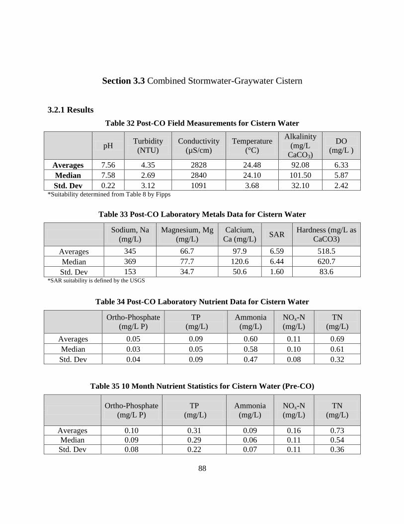
88

Section 3.3 Combined Stormwater-Graywater Cistern

3.2.1 Results

Table 32 Post-CO Field Measurements for Cistern Water

pH

Turbidity

(NTU)

Conductivity

(µS/cm)

Temperature

(°C)

Alkalinity

(mg/L

CaCO3)

DO

(mg/L )

Averages 7.56 4.35 2828 24.48 92.08 6.33

Median 7.58 2.69 2840 24.10 101.50 5.87

Std. Dev 0.22 3.12 1091 3.68 32.10 2.42 *Suitability determined from Table 8 by Fipps

Table 33 Post-CO Laboratory Metals Data for Cistern Water

Sodium, Na

(mg/L)

Magnesium, Mg

(mg/L)

Calcium,

Ca (mg/L) SAR

Hardness (mg/L as

CaCO3)

Averages 345 66.7 97.9 6.59 518.5

Median 369 77.7 120.6 6.44 620.7

Std. Dev 153 34.7 50.6 1.60 83.6 *SAR suitability is defined by the USGS

Table 34 Post-CO Laboratory Nutrient Data for Cistern Water

Ortho-Phosphate

(mg/L P)

TP

(mg/L)

Ammonia

(mg/L)

NOx-N

(mg/L)

TN

(mg/L)

Averages 0.05 0.09 0.60 0.11 0.69

Median 0.03 0.05 0.58 0.10 0.61

Std. Dev 0.04 0.09 0.47 0.08 0.32

Table 35 10 Month Nutrient Statistics for Cistern Water (Pre-CO)

Ortho-Phosphate

(mg/L P)

TP

(mg/L)

Ammonia

(mg/L)

NOx-N

(mg/L)

TN

(mg/L)

Averages 0.10 0.31 0.09 0.16 0.73

Median 0.09 0.29 0.06 0.11 0.54

Std. Dev 0.08 0.22 0.07 0.11 0.36

89

Table 36 10 Month Bacterial Sample Statistics for Cistern Water (Pre-CO)

Total Coliform

(cfu per 100 mL)

E. Coli

(cfu per 100 mL)

Enterococci

(cfu per 100 mL)

Average 194.2 5.6 138.5

Median 241.6 0.0 141.36

Std. Dev. 76.5 15.0 95.81

3.2.2 Discussion

From the cistern water data in the previous section (Tables 32-36), it can be concluded that the

cistern water is acceptable for its intended applications at the FSGE. The pH, alkalinity,

turbidity, DO, and temperature are consistent and acceptable values for typical non-potable

use. The nutrient concentrations are well below discharge standards, but at the same time the

presence of nitrogen and phosphorus will be beneficial for vegetative uptake and synthesis

during irrigation events. The high sodium concentration is acceptable for the salt tolerant

plants that are native to the subtropical climate of Florida, and more specifically the coastal

regions.

Monitoring of the HPC bacterial count of the combined cistern was performed during pre-CO

conditions and established that there were low, if any, fecal coliform or E. Coli in the cistern

water. The graywater is filtered and disinfected with ozone with an oxidation reduction

potential (ORP) probe to assure the ORP is above the required 600 mV for water disinfection.

The 600 mV should sufficiently destroy the microorganisms, resulting in less than 1 cfu per

100 mL.

90

Estimated graywater/stormwater demand is at 100 gpd. The toilet demand is at least 85% of

blackwater flow; therefore 75 gpd of the 100 gpd goes to toilet use. The rest of the demand

can be attributed to irrigation and lawn use, as the laundry flow is recycled back into the

cistern.

The economic feasibility of implementing the combined stormwater/graywater cistern is

addressed through the reduction in potable water demand. The average estimated indoor water

use in gallons per day per capita (gpcd) is 69.3 (Table 1). Through the combined

stormwater/graywater cistern, the indoor water use is reduced to the four (4) month sewage

flow average of 29 gpcd. It is estimated from Table 1 that the toilet usage could be as much as

26.7% of typical indoor water use, which reduces the potable water use to 21.5 gpcd. The

amount of potable used is 47.8 gpcd. Using a fee of $4.40 per 1000 gallons

(http://www.melbourneflorida.org/utilbill/rates.htm), the estimated annual savings for the home

is approximately $230.00. Note that this does not include the irrigation demand, which could

be a significant addition to potable water demand, which could increase the amount of savings

per year.

http://www.melbourneflorida.org/utilbill/rates.htm

91

CHAPTER 4 CONCLUSIONS

Section 4.1 Onsite Septic Treatment and Disposal System

After completing the one year sample plan for the FSGE, a number of conclusions have been

established. First, conventional drain fields do not typically provide adequate conditions for

biological nutrient removal to treat wastewater to desired levels. Also, in order to accomplish

high phosphorus removal with a passive system (no recycle pumps or other mechanical

equipment) a sorption media for chemical binding is required.

The difference in capital cost for the installation of a specified filter media bed is returned with

increased useable property area because the size of a filter media bed is a quarter of the size

required for a conventional drain field. Also, a filter media bed includes sorption media and

aerobic/ anoxic zones for BNR.

Passive on-site treatment is currently one of the most sustainable and practical solutions to the

state of Florida’s nutrient issue while also considering the triple bottom line (TBL). The TBL is

a framework for encouraging institutional concern about sustainability in every aspect of future

practices. Within the framework of TBL is consideration for the impact on society, the

environment, and economic sustainability.

92

The innovative system (Bold & GoldTM

BAM sorption media filter bed) at FSGE addresses

economic sustainability, as the system has a unit cost of only $1.15 more than a conventional

drain system per 1000 gallons treated (Table 6). The actual cost of the additional B&G BAM

was about $3500. The cost savings considering the reduce cost for using less potable water was

shown to be about equal to the additional treatment cost per 1000 gallons ($4.40 for potable

water vs. $4.13 additional cost of the B&G BAM over 20 years with no increases in potable cost

over time). Also, the passive treatment system means there are no energy costs and the O&M is

equivalent to a conventional system. The life expectancy of a sorption media filter bed is

approximately 25 years. The environmental sustainability is well established throughout this

study and previous studies, as the potential for tons per day of pollutants (nutrients, TSS, and

pathogens) to be eliminated from Florida’s water bodies. Again, since the system is passive

there is no energy consumption that could directly or indirectly lead to greenhouse gas

emissions. Finally, the sorption media contains approximately 200 gallons of shredded recycled

tire that would otherwise be landfilled. The impact on society can only be viewed as positive.

Future installation of these systems in third world countries, or other areas that are in need for

practical wastewater treatment, is extremely plausible. The resources required for installation of

the Bold & GoldTM

are readily available and the installation is not complex. The systems do not

have an effect on societal activities, as they are designed as a replacement to the current

conventional system.

93

Figure 23 Triple Bottom Line Diagram

The simplicity of the passive system makes them ideal for the general population. At the same

time, it is recognized that even with passive treatment, septic tanks are still one of the more

significant contributors to nutrient pollution. The fact is that there are 2.68 million septic tanks

and the estimated nutrient concentration in the effluent is an order of magnitude higher than the

average wastewater treatment plant. The focus should be made to bring all contributing sources

of nutrient loadings to equally low concentrations. The technology is there to bring OSTDS

effluent concentrations below 10 mg/L TN, the design and implementation just need to be

aligned.

94

Section 4.2 Graywater/Stormwater Cistern

The water quality in the cistern presents no hazards for non-potable applications. The pre-CO

bacterial analysis showed that the stormwater and graywater had no fecal coliform present. The

nutrient concentrations do not present in threats to groundwater contamination, and the high

salinity does not adversely impact the vegetation or soils.

The only issues are the observation of scale formations in the toilets and the anticipated potential

for increased demand for soaps and detergents because of the high salt content, or hardness. A

control measure for this could be a softener, or an increase in the graywater/stormwater input

into the system.

Section 4.3 Recommendations for Future Work

The primary goal over the next decade should be to get OSTDS treatment levels down to levels

comparable to wastewater treatment plants. From this study came a number of recommendations

to improve OSTDS. The first recommendation is to split the 3500 gallon septic tank into two (2)

zones. The first two-thirds (2/3’s) of the septic tank will remain the anaerobic zone. The last

one-third (1/3) will be an aerobic zone with diffuser bubbles to help generate ideal conditions for

Nitrosomonas and Nitrobacter to stabilize and grow in aerobic zone of the sorption media filter

bed.

95

Another alternative is to try and establish Ammonia Oxidizing Archaea (AOA) in the septic tank.

Although, it is reported by Ye and Zhang, 2011, that AOB are much more competitive than AOA

in high ammonium environments. The results from the study suggest that AOA have less impact

than AOB in nitrification reactors. Other studies found that AOA is the predominate

microorganism in bioreactors and in natural soils.

Recommendations for future work include PCR analysis for the determination of bacteria in the

sorption media soil. Other recommendations include direct flow monitoring throughout the

home to quantify the demand from each source in the entire pipe network of the home.

96

APPENDIX A: FSGE DATA SET

97

Table 37 List of Bacteria Data for FSGE OSTDS

Date Collected Sample Description Fecal Coliform

(cfu per 100 mL)

E. Coli

(cfu per 100 mL)

11/16/2009

E1 5,000.00 4,200.00

E3 < 1 < 1

E7 < 1 < 1

E4 < 1 < 1

12/30/2009

E1 < 1 < 1

E3 < 1 < 1

E7 < 1 < 1

E4 < 1 < 1

1/26/2010

E1 < 1 < 1

E3 8.00 4.00

E7 < 1 < 1

E4 < 1 < 1

2/10/2010

E1 551.00 496.00

E3 < 1 < 1

E7 < 1 < 1

E4 < 1 < 1

3/11/2010

E1 < 1 < 1

E3 < 1 < 1

E7 283 -115.6

E4 < 1 < 1

4/15/2010

E1 52,000,000.00 38,400,000.00

E3 4,900.00 81.00

E7 293 263

E4 35.00 < 1

5/18/2010

E1 14,000,000.00 13,200,000.00

E3 4.00 < 1

E7 8 4

E4 < 1 < 1

7/20/2010

E1 2,900,000.00 2,600,000.00

E2 1,523.00 985.00

E3 30 11

E4 4.00 <1

98

Post-CO Data

10/08/2010

E1 19200000 14266667.0

E2 48000 36900.0

E3 254 148.0

E4 204 136.0

E5 22 15.0

11/09/2010

E1 53,000.00 22,000.00

E2 54,600.00 43,600.00

E3 81.00 73.00

E4 106.00 67.00

E5 - -

12/09/2010

E1 260,000.00 55,000.00

E2 13,500.00 8,400.00

E3 27.00 8.00

E4 26.00 11.00

E5 - -

E6 - -

1/13/2011

E1 956,522.00 490,000.00

E2 29,200.00 4,900.00

E3 148.00 4.00

E4 0.00 0.00

E5 - -

2/10/2011

E1 2,000,000.00 1,660,870.00

E2 54,000.00 8,400.00

E3 96.00 15.00

E4 0.00 0.00

E5 - -

3/08/2011

E1 2,200,000.00 2,020,000.00

E2 8,200.00 1,460.00

E3 172.00 64.00

E4 0.00 0.00

E5 0.00 0.00

99

4/07/2011

E1 3,300,000.00 3,200,000.00

E2 47,200.00 18,000.00

E3 46.00 4.00

E4 4.00 0.00

E5 - -

E6 22,800.00 10,150.00

5/05/2011

E1 4,200,000.00 290,000.00

E2 79,200.00 25,000.00

E3 3,700.00 208.00

E4 88.00 42.00

E5 - -

E6 44,400.00 41,400.00

6/06/2011

E1 3,800,000.00 932,740.00

E2 63,200.00 39,600.00

E3 12.00 4.00

E4 4.00 0.00

E5 - -

E6 59,200.00 39,600.00

7/07/2011

E1 3,400,000 1,382,609

E2 52,800 50,400

E3 854 815

E4 15 4

E5 35 4

E6 28,200 26,400

8/03/2011

E1 2,266,667 550,000

E2 11,333 7,600

E3 196.00 168.00

E4 156.00 48.00

E5 23.00 0.00

E6 10,800.00 4,000.00

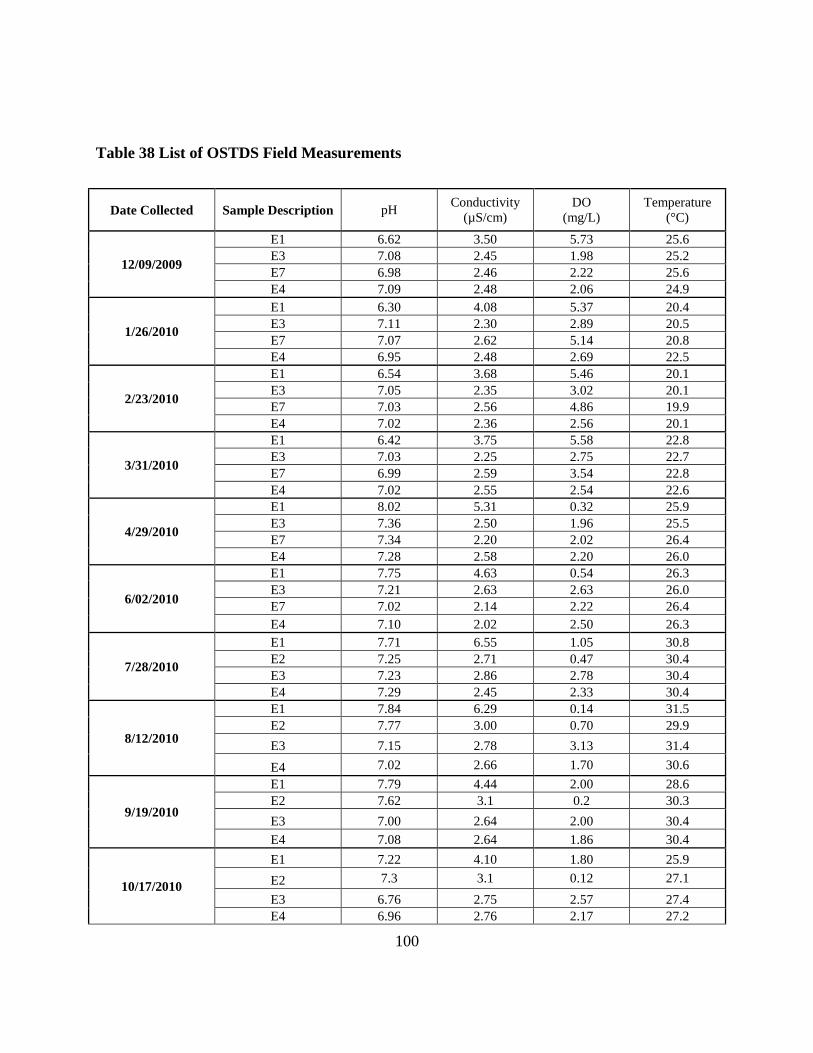
100

Table 38 List of OSTDS Field Measurements

Date Collected Sample Description pH Conductivity

(µS/cm)

DO

(mg/L)

Temperature

(°C)

12/09/2009

E1 6.62 3.50 5.73 25.6

E3 7.08 2.45 1.98 25.2

E7 6.98 2.46 2.22 25.6

E4 7.09 2.48 2.06 24.9

1/26/2010

E1 6.30 4.08 5.37 20.4

E3 7.11 2.30 2.89 20.5

E7 7.07 2.62 5.14 20.8

E4 6.95 2.48 2.69 22.5

2/23/2010

E1 6.54 3.68 5.46 20.1

E3 7.05 2.35 3.02 20.1

E7 7.03 2.56 4.86 19.9

E4 7.02 2.36 2.56 20.1

3/31/2010

E1 6.42 3.75 5.58 22.8

E3 7.03 2.25 2.75 22.7

E7 6.99 2.59 3.54 22.8

E4 7.02 2.55 2.54 22.6

4/29/2010

E1 8.02 5.31 0.32 25.9

E3 7.36 2.50 1.96 25.5

E7 7.34 2.20 2.02 26.4

E4 7.28 2.58 2.20 26.0

6/02/2010

E1 7.75 4.63 0.54 26.3

E3 7.21 2.63 2.63 26.0

E7 7.02 2.14 2.22 26.4

E4 7.10 2.02 2.50 26.3

7/28/2010

E1 7.71 6.55 1.05 30.8

E2 7.25 2.71 0.47 30.4

E3 7.23 2.86 2.78 30.4

E4 7.29 2.45 2.33 30.4

8/12/2010

E1 7.84 6.29 0.14 31.5

E2 7.77 3.00 0.70 29.9

E3 7.15 2.78 3.13 31.4

E4 7.02 2.66 1.70 30.6

9/19/2010

E1 7.79 4.44 2.00 28.6

E2 7.62 3.1 0.2 30.3

E3 7.00 2.64 2.00 30.4

E4 7.08 2.64 1.86 30.4

10/17/2010

E1 7.22 4.10 1.80 25.9

E2 7.3 3.1 0.12 27.1

E3 6.76 2.75 2.57 27.4

E4 6.96 2.76 2.17 27.2

101

11/09/2010

E1 8.10 3.95 5.40 22.8

E2 7.80 2.99 0.14 23.7

E3 7.18 2.79 2.51 23.7

E4 7.11 2.74 3.08 22.4

E5 6.77 2.90 6.80 24.5

12/09/2010

E1 8.03 2.77 3.70 24.4

E2 7.73 3.19 0.20 19.6

E3 7.19 2.65 1.79 19.8

E4 7.45 3.42 3.08 20.0

1/13/2011

E1 7.48 4.79 3.94 15.9

E2 7.53 2.57 0.32 15.8

E3 7.25 2.41 2.40 16.2

E4 7.40 2.59 4.51 16.3

E5 7.83 2.51 6.50 15.9

2/10/2011

E1 7.85 3.07 2.07 22.0

E2 7.51 2.45 0.09 21.6

E3 7.21 2.62 2.85 21.7

E4 7.18 2.63 2.42 22.3

E5 7.54 2.60 5.11 22.1

3/08/2011

E1 7.61 2.13 2.33 24.6

E2 7.15 2.69 0.19 24.1

E3 7.13 2.60 2.92 24.3

E4 7.21 2.25 2.42 24.6

E5 7.54 2.60 5.11 22.1

4/07/2011

E1 7.89 1.12 0.73 25.0

E2 7.36 2.30 0.15 25.1

E3 7.07 2.34 2.10 24.8

E4 7.13 2.37 2.52 25.0

E5 7.11 2.38 4.84 24.4

E6 7.89 1.12 0.73 25

5/05/2011

E1 8.74 1.99 3.23 28.7

E2 7.64 3.12 0.04 26.7

E3 7.12 2.70 2.30 27.5

E4 7.24 2.46 2.03 27.0

E5 7.68 3.12 5.76 30.0

E6 7.78 2.09 0.71 26.7

6/06/2011

E1 7.77 3.09 0.30 29.8

E2 7.43 2.8 0.13 28.6

E3 7.09 2.72 2.61 29.8

E4 7.31 2.53 2.6 29.7

E5 7.55 2.48 3.7 28.8

E6 7.66 2.87 0.44 28.8

7/7/2011

E1 7.50 1.50 1.67 31.7

E2 7.14 2.41 0.1 30.1

E3 6.79 2.44 2.67 29.2

E4 6.80 2.58 2.37 28.7

E5 6.92 2.49 3.41 28.9

102

E6 7.1 2.43 0.84 30.9

8/03/2011

E1 8.31 3.59 2.03 33.7

E2 7.87 2.59 0.08 32.8

E3 7 2.5 2.32 33.5

E4 7.34 2.45 2.93 32.2

E5 7.52 2.57 4.37 31.9

E6 7.76 2.67 1.23 33.1

103

Table 39 List of Chemical Data for FSGE OSTDS

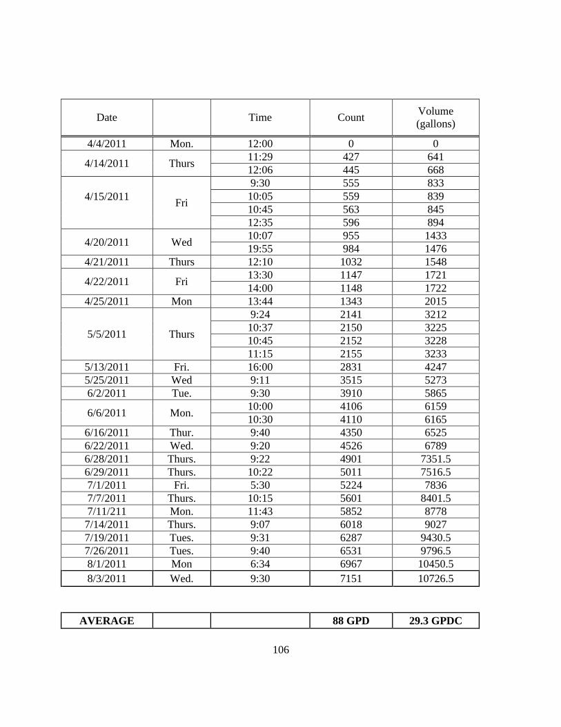
106

Date

Time Count Volume

(gallons)

4/4/2011 Mon. 12:00 0 0

4/14/2011 Thurs 11:29 427 641

12:06 445 668

4/15/2011

Fri

9:30 555 833

10:05 559 839

10:45 563 845

12:35 596 894

4/20/2011 Wed 10:07 955 1433

19:55 984 1476

4/21/2011 Thurs 12:10 1032 1548

4/22/2011 Fri 13:30 1147 1721

14:00 1148 1722

4/25/2011 Mon 13:44 1343 2015

5/5/2011 Thurs

9:24 2141 3212

10:37 2150 3225

10:45 2152 3228

11:15 2155 3233

5/13/2011 Fri. 16:00 2831 4247

5/25/2011 Wed 9:11 3515 5273

6/2/2011 Tue. 9:30 3910 5865

6/6/2011 Mon. 10:00 4106 6159

10:30 4110 6165

6/16/2011 Thur. 9:40 4350 6525

6/22/2011 Wed. 9:20 4526 6789

6/28/2011 Thurs. 9:22 4901 7351.5

6/29/2011 Thurs. 10:22 5011 7516.5

7/1/2011 Fri. 5:30 5224 7836

7/7/2011 Thurs. 10:15 5601 8401.5

7/11/211 Mon. 11:43 5852 8778

7/14/2011 Thurs. 9:07 6018 9027

7/19/2011 Tues. 9:31 6287 9430.5

7/26/2011 Tues. 9:40 6531 9796.5

8/1/2011 Mon 6:34 6967 10450.5

8/3/2011 Wed. 9:30 7151 10726.5

AVERAGE 88 GPD 29.3 GPDC

107

Figure 24 FSGE Irrigation Cistern Calibration Curve

108

Date pH (on-site) Turbidity

(NTU)

Conductivity

(µS/cm)

Temperature

(°C)

Alkalinity

(mg/L

CaCO3)

Dissolved

Oxygen

(mg/L )

1/21/2009 7.87 1.98 2490 23.9 76 8.09

1/26/2009 7.76 3.1 3610 20.8 118 11.71

2/12/2009 7.64 8.6 3220 20.0 75 9.75

3/31/2010 7.45 10.6 2450 21.1 22 7.89

4/29/2010 7.18 1.72 1283 23.7 37 6.57

6/2/2010 7.48 2.14 3650 25.1 97 5.87

6/28/2010 7.58 7.8 4290 27.8 116 3.57

7/27/2010 7.48 2.28 1200 31.8 120 3.65

8/12/2010 7.25 2195 29.1 7.09

9/19/2010 7.6 5.06 3710 27.3 122 2.33

10/7/2010 7.14 1465 25.3 82 5.70

11/9/2011 7.84 1.36 4300 24.1 119 5.20

12/9/2011 7.56 1.1 3324 23.4 98 4.4

1/13/2011 7.76 6.4 3580 17.1 105 4.86

2/10/2011 7.52 2840 21.8 100 3.70

3/8/2011 7.58 3488 24.4 90 4.1

4/7/2011 7.7 1010 25.2 6.2

5/5/2011 7.71 3950 27.5 87 9.06

6/6/2011 7.85 2321 27.4 112 5.6

7/7/2011 7.08 2850 28.7 6.7

8/3/2011 7.75 2374 27.5 3.9

109

APPENDIX B: FSGE NUTRIENT SAMPLING STANDARD

OPERATING PROCEDURE (SOP)

110

1. SCOPE AND APPLICABILITY

This Standard Operating Procedure (SOP) defines the procedures to be followed for the

collection and handling of nutrient samples at the Florida Showcase Green Envirohome (FSGE).

2. EQUIPMENT AND REAGENTS

The following is a list of equipment required to be used during analysis:

One (1) Masterflex L/S Peristaltic Pump

with Easy Load II Pump Head

Six (10) 1 liter amber jars

Twelve (12) waterproof labels

One gallon of D.I. water

Hach model HQ40d Dual Input pH/

Conductivity/ Temperature/ Dissolved

Oxygen meter.

PHC101 Standard pH Probe

CDC401 Standard Conductivity Probe

Coleman Cooler

Sample tubing

Dipper pole

LDO101 Standard Dissolved Oxygen

Probe

One (1) sample container filled with

D.I. to record temperature of samples.

Kim wipes

D.I. rinse bottle

Nitrile gloves

5-micron filters

50 mL LDPE sample container with

screw cap

50 mL plastic cups for measuring pH,

conductivity, temperature, and DO

5-micron filter paper

Suction vacuum for filtering

Suction glass for sample collection

250 mL measuring glass

111

3. COLLECTION PROCEDURE

The following section describes the collection method to be followed for nutrient sampling:

1. Give a 24 hr notice to ERD lab including the amount and type of samples that need to be

tested. (407-855-9465) Give Mark Baker notice to put cap on influent trough.

2. Pick up the peristaltic pump, Hach pH/Conductivity/Temperature/ DO meter, and other

equipment listed from the UCF CECE Chemical/Biological Process Lab (ENG 2 438).

3. Before arriving at FSGE (220 Coral Way W, Indialantic, FL), pick up a bag of ice to chill

samples to 4o C after sampling.

4. Once at FSGE, turn on the Hach meter, plug in the pump with an extension cord, and

write labels for samples.

5. The sample labels should contain: Samplers name, the project (Envirohome), the sample

location (ex. E1), the date, and the time the sample was collected. There should be Labels

for the septic samples (E1-6) and one for each the cistern and well.

6. Begin pumping from the influent for 2 hrs between 7-9 am, then 11-1, and 5-8 pm.

Combining samples at the end to make one composite sample.

7. Begin pumping a sample from location E4 using the tubing that is stored at that station

8. After the 1 liter amber bottle is filled, fill the 50 mL plastic cup for pH, conductivity,

temperature, and DO measurements.

9. Pump D.I. water through the tubing for 5-10 seconds to rinse out the septic water

10. Place the probes into the 50 mL cup and record the pH, conductivity, temperature, and

DO. Record into field data book. Rinse probes with DI water and wipe with Kim wipes.

11. Repeat steps 7 through 10 for station E2 (Collect from dipper tray)

12. Repeat steps 7 - 10 for station E1 (Collect from trough). Rinse tubing for 20-30 seconds

13. Repeat steps 7 through 10 for station E3, making sure to collect from the tubing with the

green electrical tape on it.

14. Collect a sample from the cistern using the on-site dipper pole, use the 50 mL sample to

measure and record water quality parameters (step 10).

15. Collect a sample from the well faucet. Open the valve and let the water run for a couple

112

minutes before collecting sample. Collect a 50 mL sample and perform step 10.

16. Place all samples in cooler and chill them with the bag of ice. Return to UCF

4. HANDLING PROCEDURE

This section describes the handling method to be followed for the septic samples (E1-4):

1.

2. Take the samples back to the CECE Chemical/Biological Process Lab (ENG 2 438)

3. Pour 200 mL of each sample into separate 250 mL beakers (properly labeled)

4. Collect twelve 50 mL sample bottles with screw tops (Three for each location)

5. Label each sample bottle with the following: sampler name, project name, sample

Location, date, and time. Also include either F (filtered), A (Acidified), or FA (both)

6. Filter 150 mL of the E1 beaker using the lab suction vacuum, and a 5 micron filter

paper.

7. Pour the filtered sample into appropriate 50 mL bottles (F and FA).

8. Pour the remaining 50 mL left in the beaker into the “A” sample bottle

9. Add 120 µL of concentrated (98%) Sulfuric Acid (H2SO4) into the “A” and “FA”

sample

10. Acid wash and rinse all instruments and equipment used and repeat for the remaining

samples

Place all of the sample bottles (including ambers) into the cooler and drop off at

Environmental Research and Development (ERD).

3419 Trentwood Blvd., Suite 102, Orlando, FL 32812

113

APPENDIX C: FSGE BIOLOGICAL SAMPLING STANDARD

OPERATING PROCEDURE (SOP)

114

1. SCOPE AND APPLICABILITY

This Standard Operating Procedure (SOP) defines the procedures to be followed for the

collection and handling of biological samples at the Florida Showcase Green Envirohome

(FSGE).

2. EQUIPMENT AND REAGENTS

The following is a list of equipment required to be used during analysis:

One (1) Masterflex L/S peristaltic pump

with Easy Load II Pump Head

Six (6) Corning coliform water test

sample containers, sterile with Sodium

Thiosulfate tablet (120 mL)

Two (2) Coliform water test sample

containers, sterile without sodium

thiosulfate (120 mL)

Twelve (16) waterproof labels

One gallon of D.I. water

Coleman Cooler

Sample tubing

Dipper pole

One (1) sample container filled with

D.I. to record temperature of samples.

Nitrile gloves

3. COLLECTION PROCEDURE

The following section describes the collection method to be followed for nutrient sampling:

17. Give a 24 hr notice to ERD lab including the amount and type of samples that need to be

tested. (407-855-9465)

18. Give a 24 hr notice to Mark Baker, so he can place the plug onto the end of the influent

trough. This is done to create a composite influent sample.

19. Pick up the cooler, gloves, and other necessary equipment listed in section 2.0 from the

UCF CECE Chemical/Biological Process Lab (ENG 2 438).

20. Before arriving at FSGE (220 Coral Way W, Indialantic, FL), pick up a bag of ice to chill

samples to 4o C after sampling.

21. Once at FSGE write labels for samples. The sample labels should contain: Samplers

name, the project (Envirohome), the sample location (ex. E1), the date, and the time the

sample was collected. There should be labels for the septic samples (E1-6) and one for

each the cistern and well water.

22. Begin pumping a sample from location E4 using the Masterflex silicone tubing that is

stored at that station.

23. After the 120 mL sample container is filled, pump D.I. water through the tubing for 10-15

seconds to rinse out the septic water.

24. Repeat steps 6 and 7 for station E2 (Collect from dipper tray)

25. Repeat steps 6 and 7 for station E1 (Collect from trough). Rinse tubing for 20-30 seconds

26. Repeat steps 6 and 7 for station E3, but make sure to connect the tubing to the tubing

with the green electrical tape on it.

27. Collect a sample from the cistern using the on-site dipper pole.

28. Collect a sample from the well faucet. Open the valve and let the water run for a couple

minutes to purge the well before collecting sample.

29. Place all of the sample bottles (including ambers) into the cooler and drop off at

Environmental Research and Development (ERD).

3419 Trentwood Blvd., Suite 102, Orlando, FL 32812

APPENDIX D: CUSTOM SOILS REPORT FOR FSGE

REFERENCES

Bauder, T.A., R. M. Waskom, and J. G. Davis (2007). "Irrigation Water Quality Criteria."

Colorado State University Cooperative Extension.

Borisova, T. and R.R. Carriker (2009). "Water Use in Florida." University of Florida IFAS

Extension,: 1-4.

Bounds, T.R. (1997). “Design and Performance of Septic Tanks.” Site Characterization and

Design of Onsite Septic Systems, ASTM STP 901, American Society for Testing Materials,

Philadelphia, 1997.

Burks, B.D. (1994). Onsite Wastewater Treatment Systems. Minnis Hogarth House, Ltd.,

Madison, WI,

Chang, N. B., Wanielista, M., and Xuan Z. (2008). Characterizing green sorption media in

vadose zone to improve nutrient removal of septic tank drain fields. Environmental

Engineering Science, in review.

Christova-Boal, D., R.E. Eden, and S. McFarlane. (1996). "An investigation into greywater reuse

for urban residential properties." Desalination 106: 391-397.

City of Melbourne. Water service rates and charges. 2009.

http://www.melbourneflorida.org/utilbill/rates.htm (accessed December 5, 2009).

Clark, S. E., R. Pitt, and R. Field. (2010). “Groundwater Contamination Potential from

Infiltration of Urban Stormwater Runoff”. Environmental and Water Resources Institute

of the American Society of Civil Engineers. ASCE Publications.

Dixon, A., D. Butler, and A. Fewkes. (1999). "Water Savings Potential of Domestic Water Reuse

Systems using Greywater and Rainwater in Combination." Water Science and

Technology 39: 25-32.

Duncan, R. R., R. N. Carrow, and M. Huck. (2000). "Understanding Water Quality and

Guidelines to Mangement." USGA Gren Section Record: 14-24.

Eriksson, E., K. Auffarth, M. Henze, and A. Ledin. (2002). "Characteristics of grey wastewater."

Urban Water 4: 85-104.

Fipps, G. (2004). "Irrigation Water Quality Standards and Salinity Management." Texas

Cooperative Extension.

FSGE. Florida Showcase Green Envirohome. 2010. http://www.fsge.net/index.html

Gilman, E. F. (2007). FPS415. Environmental Horticulture, Florida Cooperative

Extension Service, Institute of Food and Agricultural Sciences, University of Florida.

Van De Graaff, R., and R.A. Patterson (2001). “Explaining the Mysteries of Salinity, Sodicity,

SAR and ESP in On-Site Practice”. Oral Paper Presentation. Copyright Lanfax

Laboratories.

Hardin, M. (2006). "The Effectiveness of a Specifically Designed Green Roof Stormwater

Treatment System Irrigated with Recycled Stormwater Runoff to Achieve Pollutant

Removal and Stormwater Volume Reduction." Master's Thesis, Department of Civil and

Environmental Engineering, University of Central Florida.

Jefferson, B., A. Palmer, P. Jeffrey, R. Stuetz, and S. Judd. (2004). "Grey water characterisation

and its impact on the selection and operation of technologies for urban reuse." Water

Science and Technology 50: 157-164.

Johnson, G., and H. Zhang. (2006). "Classification of Irrigation Water Quality." Oklahoma

Cooperative Extension.

Katz. B.G., D.W Griffin., P. B McMahon., H. S Harden., E. Wade, R.W. Hicks and J. P. Chanton

(2010). Fate of Effluent-Borne Contaminants Beneath Septic Tank Drainfields Overlying a

Karst Aquifer, J. Environ. Qual., 39(4): 1181-1195.

Kelly, M., M. Hardin, and M. Wanielista.(2007). A Stormwater Management Evaluation of the

2007 New American Home Stormwater Treatment System and the Stormwater Academy

Green Roof. FDEP Report, Orlando: Stormwater Mangement Academy.

Lazarova, V., S. Hills, and R. Birks.(2003). "Using recycled water for non-potable, urban uses: a

review with particular reference to toilet flushing." Water Science and Technology 3: 69-

77.

Liptan, T. (2003). "Planning, Zoning and Financial Incentives for Ecoroofs in Portland, Oregon."

Greening Rooftops for Sustainable Communities, First North American Green Roof.

Chicago.

Liu, K., and B. Baskaran. (2003). "Thermal Performace of green roofs through field evaluation."

Proceedings for the First North American Green Roof Infrastructure Conference, Awards

and Trade Show. Chicago. 1-10.

Liu, Cheng and Evett, Jack B. (2000). Soil Properties: Testing, Measurement, and Evaluation.

Fourth Edition. Prentice Hall.

March, J.G., M. Gual, and J. Ramonell. (2005). "A kinetic model for chlorine consumption in

grey water." Desalination 181, no. 1-3: 267-273.

Metcalf and Eddy (2003). Wastewater engineering: treatment and reuse, 4th edition, McGraw Hill

Publishing, New York, USA.

Menneer, J.C., McLay, C.D.A., and Lee R. (2001). “Effects of Sodium-Contaminated

Wastewater on Soil Permeability of Two New Zealand Soils”. Australian Journal of Soil

Res. Volume 39, pgs. 877-891.

Monterusso, M. (2003). "Species Selection and Stormwater Runoff Analysis from Green roof

System." Department of Horticulture, Michigan State University.

National Science Foundation. (2007). “Wastewater treatment systems-Nitrogen reduction.” NSF

International Standard/American National Standard.

National Science Foundation International (2009). Relevant Standards and Protocols. NSF/ANSI

Standards 245: Wastewater Treatment Systems - Nitrogen Reduction.

http://www.nsf.org/business/wastewater_certification/standards.asp?program=WastewaterCe

r#245

Niachou, A., K. Papakonstantinou, M. Santamouris, A. Tsangrassoulis, and G. Mihalakakou.

(2001). "Analysis of the green roof thermal propertiesand investigation of its energy

performance." Energy and Buildings 33: 719-729.

Onmura, S., M. Matsumoto, and S. Hokoi. (2001). "Study on evaporative cooling effect of roof

lawn gardens." Energy and Buildings 33, no. 7: 653-666.

Pitt, R., and A. Maestre. (2004). "The National Stormwater Quality Database (NSQD, version

1.1)." 1st Annual Stormwater Mangement Research Symposium Proceedings. Orlando.

13-51.

Qadir, M. and Schubert, S. (2002). “Degradation Processes and Nutrient Constraints in Sodic

Soils”. Land Degradation and Development. John Wiley & Sons, Ltd.

Rivera, B. (2010). Analysis Of The Florida’s Showcase Green Envirohome Water/Wastewater

Systems And Development Of A Cost-Benefit Green Roof Optimization Model, Master’s

Thesis, Department of Civil, Environmental, and Construction Engineering, University of

Central Florida.

Ryan, P. (2008). "Nutrient Reduction in Stormwater Pond Discharge Using a Chamber Upflow

Filter and Skimmer (CUFS)." Master's Thesis, Department of Civil, Environmental, and

Construction Engineering, University of Central Florida.

Sawyer, C. N., McCarty, P. L., and Parkin, G. F. (2003). Chemistry for Environmental Engineering

Science, McGraw-Hill, New York, USA, Fifth Edition.

Shah, T. (2007). "Fate of Nitrogen and Phosphorus Species from a Black and Gold Nugget Mix

in a Laboratory Column Simulated Septic Tank Drainfield." Master Thesis, Department

of Civil and Environmental Engineering, University of Central Florida, Orlando.

St. Johns Water Management District. (2009) "Water Restrictions: Know the designated days.”

Suarez, Donald L., Wood, James D., and Lesch, Scott M. (2006).“Effect of SAR on Water

Infiltration Under a Sequential Rain-Irrigation Management System”. Agricultural Water

Management. pgs. 150-164.

Thompson, A. (1998). "Grass-roofs movement in landscape architecture." The magazine of the

American Society of Landscape Architects, 1998: 47-51.

Todd D K, and Mays L W, (2005), Groundwater Hydrology. 3rd

Edition: John Wiley and Sons,

Inc

U.S. Environmental Protection Agency (USEPA). (2002). USEPA Onsite Wastewater Treatment

Systems Manual, EPA/625/R-00/008, Office of Research and Development, Washing ton

DC, USA.

United States Environmental Protection Agency (USEPA (1988). Design manual-constructed

wetlands and aquatic plant systems for municipal wastewater treatment, EPA/525/1-88/022,

US Environmental Protection Agency, Center for Environmental Research Information,

Cincinnati, OH.

United States Geological Survey. (1992). Florida's Ground Water Quality Monitoring Program.

Tallahassee: Florida's Geological Survey.

Wanielista, M., F. Kelly, and M. Hardin. (2006). "Effectiveness of a Greenroof Irrigation System

Irrigated with Filtrate from a Greenroof." Final Report, State of Florida Department of

Environmental Regulation, Tallahassee.

viability study of a residential integrated stormwater

Documents