vibration analysis of a vawt leyre redín larrea
TRANSCRIPT

Supervisor:
Professor STOYAN TASHKOV
Vibration Analysis of a VAWT Leyre Redín Larrea
MASTER THESIS INDUSTRIAL ENGINEERING
28/05/2013

Vibration Analysis of a VAWT Leyre Redín Larrea
2
TECHNICAL UNIVERSITY OF SOFIA
ENGLISH LANGUAGE FACULTY OF ENGINEERING
Deadline: ……………… Dean: ………………………………
Name: Prof. Dr. Tasho Tashev
RESEARCH PROJECT ASSIGNMENT
MEng course
1. Student’s name: LEYRE REDÍN LARREA Faculty No: …………………
2. Project title: Vibration Analysis in a Vertical Axis Wind Turbine
3. Basic project specifications: Developing a Matlab program which calculates the vibration and stress in a vertical axis wind turbine tower. Comparing the results with real measurements in a VAWT prototype.
4. Contents:
a) Acknowledgements b) Abstract c) Aim of the thesis d) Vertical Axis Wind Turbines introduction e) Vibration fundaments f) Methodology: Modeling Vertical Axis wind turbines in Matlab g) Vibration analysis h) Compiling in C++ i) Measurements and results j) Conclusions k) Annexes l) References
Project supervisor: …………………………….. Deputy Dean: ………………………
Name: Prof. Stoyan Tashkov Name: Assoc. Prof. Dr. R. Dinov
Consultant: …………………………………….
Name: Prof. Julian Genov
Vibration Analysis of a VAWT Leyre Redín Larrea
3
CONTENTS 1. Acknowledgements ................................................................................. 4
2. Abstract ................................................................................................... 5
3. Aim of the thesis ..................................................................................... 6
4. Introduction to Vertical Axis Wind Turbines ......................................... 8
5. Vibration fundamentals ......................................................................... 14
6. Methodology: modeling VAWT in Matlab .......................................... 16
6.1 WIND MODEL ...................................................................................... 16
6.2 BLADE MODEL .................................................................................... 24
6.3 GENERATOR MODEL ............................................................................ 40
6.4 TOWER MODEL .................................................................................... 42
7. Vibration analysis ................................................................................. 43
7.1 ONE DIMENSIONAL PROBLEM ............................................................. 43
7.2 TWO DIMENSIONAL PROBLEM ............................................................ 52
7.3 VIBRATION ANALYSIS IN MATLAB ...................................................... 63
8. Compiling in c++ .................................................................................. 73
9. Measurements and results ..................................................................... 74
10. Conclusions ........................................................................................... 78
11. Annexes ................................................................................................. 82
11.1 Uni-T UT372 Digital tachometer sheet data .................................... 82
11.2: Compact daq-9174 National Instrument data sheet ........................ 83
11.3: Accelerometer KD35 ...................................................................... 86
12. References ............................................................................................. 87

Vibration Analysis of a VAWT Leyre Redín Larrea
4
1. ACKNOWLEDGEMENTS First of all I would like to thank my supervisor, Professor Stoyan Tashkov for his
continued guidance, support and encouragement during my project work. His
experience and theoretical background were fundamentally important for my work
described in this thesis. I would also like to show my appreciation to Professor Kalin
Adarsky for his help and patience throughout the completion of this project. Also I
would like to thank all the professors that take part in the Mechanical department
because they have been kind and helpful with me.
I would like to thank my coordinator, Professor Vladislav Slavov for his infinite help
since we arrived to Sofia and his day-by-day care.
I would like to show my appreciation for the support of Tasho Tashev who helped me
find the most suitable area for my master thesis and for his concern that everything was
well.
I would like to thank also my University, Universidad Pública de Navarra, and the
Technical University of Sofia, for giving me the chance to study one year abroad. It has
been a wonderful experience studying in TUS, meeting new people, discovering a new
culture and improving my language skills by learning Bulgarian and improving my
English.
Finally I would like to thank my family and friends for supporting me everyday,
encouraging me when something was not going well and for their day-by-day care.

Vibration Analysis of a VAWT Leyre Redín Larrea
5
2. ABSTRACT This research analyses the vibrations in a special type of vertical axis wind turbine with
parabolic blades called Darrieus. The study will be focused on the vibrations of the
tower. It is really important to know the tower´s behaviour against them in order to
choose the best material for it and to avoid problems such as frequent maintenance and
even wind turbine breakage.
For developing this thesis a vast array of information has been gathered from technical
sources regarding vertical axis wind turbines. For modeling the wind turbine, the
Matlab program was used in order to design the behaviour of the wind turbine. The
vibrations were calculated using a finite element method. An important step before
calculating the tower vibrations is the study of the resulting forces at different points in
each blade, which are due to the blade rotation.
Once the vibration results were obtained they were compared with the real
measurements carried out in a vertical axis wind turbine prototype. They were measured
using a National Instrument device. It has four very sensitive sensors that were located
in the tower in order to measure its vibrations. Besides, for the data acquisition, we
connected the device to a computer that has LabVIEW Signal Express software and we
analyzed the results.
The conclusion is that our designed program is reliable as the real measurements are
very close to the ones obtained with Matlab.
Keywords: Vertical axis wind turbine (VAWT), vibrations, Matlab programming,
measurements.

Vibration Analysis of a VAWT Leyre Redín Larrea
6
3. AIM OF THE THESIS Wind energy is considered one of the most viable sources of sustainable energy. Its
rapid growth in recent years has gained research attention aimed at investigating
emerging problems. In the past, most of the research has concentrated on domains such
as wind energy conversion, prediction of wind power, wind speed prediction, wind farm
layout design, and turbine monitoring. Despite its impact on the performance and
lifetime of wind turbines, the published research on wind turbine vibrations is rather
limited. Mitigating the vibrations of a wind turbine can potentially prevent material
fatigue, reduce the number of component failures, and extend the life cycle of some
components. This in turn converts into increased turbine availability and reduced
maintenance costs.
Therefore, the aim of this thesis is to develop a program capable of calculating the
vibrations of the wind turbine’s tower in an accurate manner. This topic was chosen
because vibrations are a really important factor to consider while modeling a wind
turbine. As far as the wind turbine behaviour against vibrations is known, you can
choose the best material to build it and decrease the maintenance costs. Also you can
predict the wind turbine behaviour anticipating possible breaking.
Modeling turbine vibrations is complex, as many parameters are involved. The most
important are: wind speed, wind turbulence, blade profile, generator, tower´s length, and
tower’s geometry. For developing the target, a program has been carried out in Matlab
that models a vertical axis wind turbine. The user introduces the input data and the
program calculates the tower vibrations. In addition to this, it can also plot other outputs
such as wind speed, torque and thrust force for each blade and stress in the tower.
For modeling the wind turbine, the study will differentiate the main components which
are: wind, blade, generator and tower. Each part will be described theoretically. Besides
this, it will be explained how to implement this in Matlab.
Another goal is to develop a nice GUI interface in Matlab which will facilitate the user
the interpretation of the results with no need to understand the Matlab complicated
code. Also, it will be exported to an exe file so that Matlab installation is not needed to
run the program. It will be compiled in C++, which will enable the program to be used
in every computer in the world.

Vibration Analysis of a VAWT Leyre Redín Larrea
7
This thesis is based on a vertical axis wind turbine prototype that we have in the
Mechanic´s laboratory. This allows for comparison of the Matlab results with reality,
measuring in the prototype. It was used a National Instrument CompactDAQ-9174
which has four sensors connected to the tower. Therefore, the accelerometers were able
to measure the vibrations in different parts of the tower. For analyzing the results, the
device was connected to a laptop with LabVIEW Signal Express software installed.
These experiments and their results will be explained carefully in another chapter of the
thesis.
Therefore, the main target is to calculate the vibrations in the designed Matlab program
and compare them with the others measured on the vertical axis wind turbine prototype.

Vibration Analysis of a VAWT Leyre Redín Larrea
8
4. INTRODUCTION VERTICAL AXIS WIND TURBINES
A sustainable future with limited atmospheric CO2 emissions and growing energy needs
forces us to consider alternative energy sources to oil, gas and coal.
The situation is more than worrying, as the impact on the Earth climate will be
incurable without a swift move to clean energy.
In 2007 [1], the electrical power generation accounted for 29% of the atmospheric CO2
emissions. Reducing this source will not solve the problem but can significantly
contribute to its solution. None of the CO2 free technologies that are technically mature
today, or in the near future can on its own tackle the problem. A global solution must
also provide capacity to match the fluctuating demand. Therefore storage and
transmission networks are also key factors.
Wind power is a strong candidate towards a sustainable future: wind power with hydro
power are among the most cost effective renewable energies. For many countries, with
its relatively fast development potential, wind power represents a good starting point for
developing renewable energy sources. However, due to its variability, it cannot aim to
be the only electricity source for a single country.
Wind power has been commercially successful in Europe for more than a decade.
European countries have more than 90 GW installed capacity with 6 top leading
countries [2]: Germany with 29.06 GW, Spain 21.67 GW, Italy 6.75 GW, France 6.8
GW, UK 6.54 GW and Portugal 4.08 GW. Bulgaria for instance has 612MW installed,
but they are trying to reach 3GW by 2020 [3]. Although Europe has been the number
one region when it comes to new yearly installed capacity for more than a decade, the
United States, China and Japan are now moving ahead. In Europe, offshore wind power
opens a new arena for wind developments, especially in the North Sea.
The world’s leading manufacturers were originally situated in countries where local
incentives have accelerated the installation of turbines such as Germany, Denmark and
Spain. Now fast emerging markets like the US, China and India have pushed strong
local suppliers. The market leaders are today [1]: GE Energy (US) 15%; Vestas
(Denmark) 12.5%; Sinovel (China) 9.2%; Enercon (Germany) 8.5%; Goldwind
(China) 7.2% and Gamesa (Spain) 6.7%.

Vibration Analysis of a VAWT Leyre Redín Larrea
9
In terms of technology, the market is dominated by three bladed upwind horizontal axis
wind turbines (HAWTs) with gearbox and asynchronous generators. The current thesis
will focus on a less well known but emerging technology, the vertical axis wind turbines
(VAWTs). In particular this thesis will be focused on a special type of VAWT with
straight blades also referred to as straight-bladed Darrieus rotor or as H rotor, the H
representing its cross vertical section.
This turbine is omni-directional and needs no yaw mechanism. Due to the straight
blades, a simple blade profile can be used. The axis orientation enables the generator to
be placed on the ground. The H-rotor concept studied here is of the direct drive type, the
shaft is directly connected to the generator, thus eliminating the need for a gearbox. This
concept enables a lighter tower structure. Furthermore, the H-rotor shows a lower
optimal tip speed ratio limiting the noise emissions. The use of electrical controlled
passive stall regulation does not require pitching the blades.
The H-rotor with generator and electronic system on the ground can have a lower top
mass than HAWTs. This has two advantages [1]:
More mass generates more cost. The low mass allows minimizing the turbine
cost including the foundation cost.
Optimization of installation costs. The H-rotor concept can access markets in
developed countries with limited crane capacity. Thus limiting again the capital
investment cost through cheaper installation.
The low tower head mass can be a crucial advantage for offshore applications or
onshore applications in an area with reduced crane availability. Their simplified
structure can be used to optimize mass production costs for small or remote
applications. The lack of mechanical control in conjunction with direct drive generators
placed on the ground has the potential to substantially reduce the operation and
maintenance costs. In summary, the vertical axis turbines can represent a breakthrough
for several applications.
Historical overview of wind power and VAWTs In 1888 Charles Brush built the first wind turbine to generate electricity [4]. It had a
diameter of 17 meters and 144 blades made of wood. The generator was able to produce
only 12kW due to its low efficiency.

Vibration Analysis of a VAWT Leyre Redín Larrea
10
Figure 4.1: Brush wind turbine
During the Second World War the Danish company F. L. Smidth built several
horizontal wind turbines of two and three blades [4].
Figure 4.2: Smidth HAWT
The innovating wind turbine Gedser was built in 1956 by J. Juul for the company
SEAS, in Denmark [4]. It had a power of 200kW. The wind turbine had speed control
and emergency brakes. It was one of the first designs of the modern wind turbines.
In the 70s, after the oil crisis many countries started to be interested in wind power. In
1979 two Nibe wind turbines were built, each one with a power of 630kW [4]. It was in
1980 when the wind power industry started to be more competitive, the price of the
kilowatt decreased about a 50% percent of its previous value and the wind power
industry started to be more professional.
In 1931 a French aeronautical engineer, Georges Jean Marie Darrieus, patented a
“Turbine having its shaft transverse to the flow of the current”, it had a power of
10kW[5]. Darrieus patent also included curved blades to avoid the bending due to
centrifugal forces.
It is one of the most common vertical axis wind turbines and there was also an attempt
to implement the Darrieus wind turbine on a large scale effort in California by the

Vibration Analysis of a VAWT Leyre Redín Larrea
11
FloWind Corporation [5]. However, the company went bankrupt in 1997; nevertheless,
this turbine was the starting point for further studies on VAWT, to improve efficiency.
In 1931 savonius wind turbines were invented by the Finnish engineer Sigurd J.
Savonius. However, Johann Ernst Elias Bessler (born 1680) was the first to attempt to
build a horizontal windmill of the Savonius type in the town of Furstenburg in Germany
in 1745 [5]. The Savonius rotor operates at high torques and low rotation speeds that are
not favorable for electric power generation.
Figure 4.3: Straight-bladed Darrieus rotor on the left, Darrieus rotor in the middle and Savonious wind turbine on the right
Vertical axis turbines can also be used in ship propulsion as pioneered by Van Voith. A
modern development has been marketed by Voith Turbomarine GmbH company[1].
The turbine uses variable pitch blades to create a thrust force on the desired direction
improving its maneuverability.
Figure 4.5: Voith Schneider propulsion concept with vertical axis technology
The vertical axis turbine has also been applied to underwater applications:

Vibration Analysis of a VAWT Leyre Redín Larrea
12
Figure 4.6: Underwater turbine vertical axis applications
Examples In 1989 the biggest H-rotor in Europe was VAWT-850 which was built in the UK [5].
It had a height of 45m, a rotor diameter of 38m and a power output of 500kW. This
turbine had a gearbox and an induction generator inside the top of the tower. It was
installed at the Carmarthen test site during 1990 and operated until February1991, when
one of the blades broke due to an error in the manufacture of the fiberglass blades.
In the 90’s the German company Heidelberg Motor GmbH developed and built several
300 kW prototypes, with direct driven generators with large diameter [5]. In some
turbines the generator was placed on the top of the tower while in other turbines it was
located on the ground.
In 2010, the VerticalWind AB was built in Uppsala, Sweden [5]. It was the biggest
VAWT in Sweden: it is a 3 blade Giromill with rated power of 200 kW. The tower has a
wood composite material that makes the turbine cheaper than other similar structures
made by steel.
Figure 4.7: VAWT in Falkenberg, Sweden.

Vibration Analysis of a VAWT Leyre Redín Larrea
13
Another popular variation of the Darrieus design, the H-rotor design, is also being tested
offshore. Technip, a French firm that worked with Siemens and Statoil to launch
floating turbines in Norway, in 2011, launched the Vertiwind project to test a pre-
industrial prototype of 2MW [6]. They did so along with French partners Nénuphar,
Converteam, and EDF Energies Nouvelles. Technip said that the VAWT design was
ideal because it freed the turbine of constraints related to foundations of fixed wind
turbines, and it doesn’t have a yaw or pitch system, a gearbox, or complex blade
geometry. Those features result in lower installation and operation costs.
Figure 4.8: Offshore VAWT launched by Technip

Vibration Analysis of a VAWT Leyre Redín Larrea
14
5. VIBRATION FUNDAMENTALS Any repetitive motion is called either vibration or oscillation. The motion of a guitar
string, the swaying of tall buildings due to wind or earthquake, or the motion of an
airplane in turbulence are typical examples of vibrations. However, the concepts of
movement, oscillation and vibration are not the same. Every vibration is an oscillation
and every oscillation is a movement, but that is not true in the other way [7]. For
example, a wheel always moves but it doesn´t oscillate, and a pendulum always
oscillates but it doesn´t vibrate. The difference is related with the energy concept. Both
oscillation and vibration extend in time, however different kind of energies interfere in
them. Therefore, in the pendulum the interfering forms are the kinetic and the potential
energy. However, vibration requires another special energy, known as the strain energy.
When analyzing a real system, the first thing to be done is to determinate a mathematic
model of that system, in which the characteristics and physic properties of the real
model are implemented. These properties are named as parameters. The parameters of a
mechanic system are: stiffness (k), mass (m) and damping (c). They are correlated with
the most characteristic types of forces: elastic forces, inertial forces and dissipation
forces, respectively [7].
The stiffness, mass and damping are usually constant parameters that do not vary with
time or with the system deformation.
Real systems always have continuous parameters. For instance, it is not possible to have
a massless element of a machine which is deformed without a force application.
However, most of the time, approximate mathematic models can be obtained
concentrating in some elements of the characteristics of the system. For instance,
assigning all the kinetic energy to an indeformable mass. These are called discrete
systems of concentrated parameters.
There are also discrete models with distributed parameters, therefore each element has
mass, it is been deformed and it dissipates energy. These discrete systems of distributed
parameters allow a much more accurate analysis of the mathematical models of the real
system than those with concentrated parameters [7]. The Finite Element Method
(F.E.M) is a powerful tool for analyzing these problems.

Vibration Analysis of a VAWT Leyre Redín Larrea
15
Vibrations can be defined as a particular case of a mechanical system dynamics, in
which there is an exchange of elastic energy and an oscillation around an equilibrium
position [7]. It is known, from experience, that if a system is taken from its equilibrium
position and released, it begins to vibrate with an amplitude that starts to damp more or
less rapidly, depending on the facility of the system to dissipate energy. These
vibrations take place in a system in the absence of exterior forces. They are only caused
by certain initial conditions such as velocity and/or displacement. These are called free
vibrations [8].
On the contrary, the vibrations that occur because of the appearance of varying forces
with the time are called forced vibrations. These can be classified according to the
variation in time of the excitation forces [7]:
‐ Harmonic excitation. They vary sinusoidally.
‐ Periodic excitation. They repeat values periodically.
‐ Pulses. They are very intense forces acting during infinitesimal times.
‐ Forces that vary in an arbitrary manner with time. It is the most general case.
These include; mobile forces on the system or harmonic excitations of variable
frequency.
Dynamic deformations are those that vary with time. A dynamic system is steady when
its variation with time has a periodic character. However, a dynamic system is transient
when its variation with time is random [7].
Deterministic vibrations are those that occur when the applied forces are known.
However, this is not the ordinary real situation, for instance the efforts that absorb the
suspension of a car over a bad road or those which suffer the wings of a plane while a
storm. Generally, they cannot be assumed to be known. Actually, in these and other
similar cases, statistical values of the applied forces are used, such as its average or
variance. The random vibration theory studies these cases and manages to link statistical
values of the response with the statistical values of the excitation [8].

Vibration Analysis of a VAWT Leyre Redín Larrea
16
6. METHODOLOGY: MODELING VAWT IN MATLAB 6.1 WIND MODEL
Wind turbines produce a complex and continuous fluctuating power. A large part of the
complexity resides on the input: the wind. The main source of power variation on
conventional wind turbines is the wind speed variation.
Mainly there are two patterns that explain wind variation: variation in space and
variation in time.
6.1.1 WIND VARIATION IN SPACE Wind variation in space is basically due to two factors [10]:
‐ Global and local wind systems.
Global circulation is due to Coriolis’ force that is a fictitious force that deviates
particles to the right side in the North hemisphere and to the left side in the South
hemisphere [9]. It is important on a global scale, because locally, it is a weak
force compared to others.
Figure 6.1.1 Wind global circulations due to Coriolis´ force
Wind variation is also caused by meso-scale factors such as sea breeze, mountain
breeze or Foehn effect. Sea breeze is originated because of the Earth´s
temperature, which during the day is warm and drops at night. As the sea
temperature is different and mostly constant, an air flow appears and during the
day it goes in one direction and at night in the opposite.

Vibration Analysis of a VAWT Leyre Redín Larrea
17
Figure 6.1.2 Sea breeze
The Foehn effect is a warm, strong, and often a very dry downslope wind that
descends in the lee of a mountain barrier [10].
Figure 6.1.3 Foehn effect.
Terrain complexity also causes wind variation. The parameter of turbulence −t− is
defined as the standard deviation of the wind velocity divided by the medium
wind speed [10]. In abrupt terrains, the medium wind speed is higher than in flat
areas and the velocity distribution is also more irregular. Therefore, turbulence is
lower in plain terrains than in mountainous ones.
Figure 6.1.4: Comparison between turbulence in complex terrain (20%) and in plain
terrain (5%) [10]

Vibration Analysis of a VAWT Leyre Redín Larrea
18
‐ Wind shear profile
The wind shear profile is the change in speed of wind over a relatively short
distance [10].
Figure 6.1.5: Wind profile
The factors that influence in the rise of the wind speed with the height are the
terrain rugosity, the atmospheric stability and the orography. It is possible to
calculate the wind speed with this equation [10]:
Equation 6.1.1)
Where α is the Hellmann exponent that decreases with the rate of atmospheric
stability and it increases with the rugosity of the terrain [10].
The following table shows the relationship between the type of terrain and its
corresponding Hellmann coefficient:
Table 6.1.1: Hellman coefficient depending on the terrain [10]
Terrain α exponent
Plain (grass, ice) 0,08-0,12
Plain (sea, seaside) 0,14
Not abrupted terrain 0,13-0,16
Rustic area 0,2
Abrupted terrain or forest 0,2-0,26
Very abrupted terrain and cities 0,25-0,4
Vibration Analysis of a VAWT Leyre Redín Larrea
19
Figure 6.1.6: Wind profile depending on the type of terrain. It shows that in the city it
is needed a higher height than in an open land terrain for obtaining the same speed.
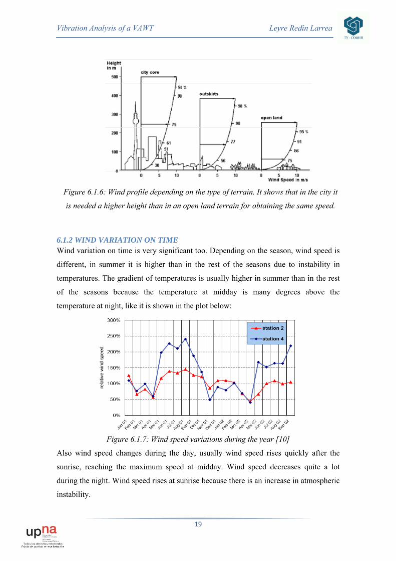
6.1.2 WIND VARIATION ON TIME Wind variation on time is very significant too. Depending on the season, wind speed is
different, in summer it is higher than in the rest of the seasons due to instability in
temperatures. The gradient of temperatures is usually higher in summer than in the rest
of the seasons because the temperature at midday is many degrees above the
temperature at night, like it is shown in the plot below:
Figure 6.1.7: Wind speed variations during the year [10]
Also wind speed changes during the day, usually wind speed rises quickly after the
sunrise, reaching the maximum speed at midday. Wind speed decreases quite a lot
during the night. Wind speed rises at sunrise because there is an increase in atmospheric
instability.

Vibration Analysis of a VAWT Leyre Redín Larrea
20
Figure 6.1.8: Variation of wind speed and wind direction during the day [10]. Probably
the peak in wind velocity at about 20h is because of a storm.
The procedure to choose the best place for placing a wind turbine is complicated due to
all these factors that affect the velocity and direction of wind. A long-term observation
(30 years) of wind speed is needed to place the wind turbine in the correct area.
Moreover, for horizontal wind turbines, it is important to know the best direction to
place the wind turbine, but it is not so important for vertical axis wind turbines because
they don´t need to be orientated to the wind direction. The wind roses, which show the
best place for the wind turbines to be placed, are developed taking this information into
account[10].
Figure 6.1.9: Wind rose (direction in red and wind power in blue)
6.1.3 MODELING WIND IN MATLAB For modeling the wind in Matlab, two aspects have been differentiated: the first one
represents a mean wind speed profile over the rotor area, defined as deterministic; and
the second one is turbulence, assumed as stochastic.
The deterministic part of the wind over the rotor area is assumed “constant” in 10
minute periods [11]. The wind variations are the time variant part that has a stochastic
behaviour. This assumption is valid only in periods up to few minutes, because above

Vibration Analysis of a VAWT Leyre Redín Larrea
21
this there is a slow wind variation in the mean wind speed, due to the continuous change
in the atmosphere.
In 10 minute periods, the stochastic and deterministic parts can be combined to express
the total wind at one position.
Deterministic Wind Model The deterministic part, as explained before, is independent of the time. It will only
influence the dynamics of the wind turbine, because the blades rotate.
The formula used in Matlab for implementing the deterministic wind model is the
following [11]:
w = Meanspeed* 1 + d.wHarm*cos Numberblades*Bladeangle
(Equation 6.1.2)
Where:
- Meanspeed is the medium wind velocity, which is introduced by the user.
- d.wHarm is the amplitude of the nth harmonic. It is calculated based on the
geometric parameters of the wind turbine, the value is 0,01.
- Numberblades is the number of blades that the wind turbine has. It is introduced
by the user.
- Bladeangle is the initial angle of the blade, which is introduced by the user.
Assuming that mean speed is 10m/s, that the number of blades is three and that the
angle of the blade is 0˚ the plot which illustrates the deterministic wind model is:
Figure 6.1.10: Plot for deterministic wind model

Vibration Analysis of a VAWT Leyre Redín Larrea
22
Stochastic Wind Model The stochastic part of the wind, in this thesis called turbulence, is the time variant part
of the wind acting on the rotor area. Turbulence is the wind speed variations in a broad
range from seconds to minutes. The variations have naturally a random behaviour but
the air dynamics creates a main pattern on the wind speed variations.
For modeling in Matlab the Stochastic wind model we should firstly apply filters [11]:
[aK, bK, cK, dK] = Kaimal( d.tau );
[a0, b0, c0, d0] = WindAdmittance(0, d.dTF );
[a3, b3, c3, d3] = WindAdmittance(3, d.dTF );
[a0, b0, c0, d0] = Series( a0, b0, c0, d0, aK, bK, cK, dK );
[a3, b3, c3, d3] = Series( a3, b3, c3, d3, aK, bK, cK, dK );
[a0, b0] = C2DZOH( a0, b0, d.dT );
[a3, b3] = C2DZOH( a3, b3, d.dT );
With Kaimal function we eliminate high frequency components [11]. The equations of
this filter are implemented in Matlab as it’s described above:
x[k+1] = a*x[k] + b*u[k]
y[k] = c*x[k] + d*u[k]
With WindAdmittance (harm, dTF) function we create a wind admittance filter [11].
x[k+1] = a*x[k] + b*u[k]
y[k] = c*x[k] + d*u[k]
Where dTF= Frequency scaling constant = Blade radius/mean wind
With Series function we connect the two filters in serie, we multiply them.
With C2DZOH function we create a discrete time system from a continuous system
assuming a zero-order-hold at the input [11]. It follows this structure:
Given: x = ax + bu
Find f and g where: x(k+1) = fx(k) + gu(k)
Secondly, we have to develop the following operations:
wR = d.sigmaWind*randn;
x1 = a0*x1 + b0*wR;
y1 = c0*x1 + d0*wR;

Vibration Analysis of a VAWT Leyre Redín Larrea
23
wR = d.sigmaWind*randn;
x2 = a3*x2 + b3*wR;
y2 = c3*x2 + d3*wR;
wR = d.sigmaWind*randn;
x3 = a3*x3 + b3*wR;
y3 = c3*x3 + d3*wR;
w = y3*cA + y2*sA + y1;
Where:
‐ d.sigmaWind is the sigma wind noise speed, it is considered a default value
−1−.
‐ randn returns an array of random values.
‐ cA= cos(Number_blades*Angle_blade)
‐ sA=sin(Number_blades*Angle_blade).
For the wind model we used this stochastic wind plus the deterministic wind [11].
wS = WindStochastic + WindDeterministic (Equation 6.1.3)
The plot of the result model assuming that mean speed is 10m/s, that the number of
blades is three and that the angle of the blade is 0˚ is:
Figure 6.1.11: Plot for stochastic plus deterministic wind model

Vibration Analysis of a VAWT Leyre Redín Larrea
24
6.2 BLADE MODEL
Different airfoils are named by their characteristic parameters, for example, the
dimensionless maximum thickness. A typical example is NACA series airfoils that
include NACA four-digit wing sections, NACA five-digit wing sections, and NACA 6
series wing sections. An airfoil shape that can be expressed analytically as a function of
three parameters is composed of a thickness envelope wrapped around a mean chamber
line [12] in the manner show on following Figure 6.2.1.
Figure 6.2.1: Naca profile with its main parameters
I will study the airfoils from the NACA four-digit (NACA abcd). These digits represent:
a= 100*maximum deflection (f)
chord line (c)
b= 10*position of the maximum thickness point in the chamber line (xc)
chord line (c)
cd= 100*maximum thickness (tmax)
chord line (c)
6.2.1 THICKNESS The current airfoil used on the wind turbine is the NACA 0018. It means that it is a
symmetric airfoil without camber.
Figure 6.2.2: NACA 0018 profile built by the software Profili

Vibration Analysis of a VAWT Leyre Redín Larrea
25
The thickness has been chosen to give enough structural strength with respect to the
loads on the blades. The advantage of higher thickness is:
• Increase of structural strength.
The disadvantages are:
• Higher drag coefficient at lower angles of attack.
• Chance of ’overshooting’ the maximum, past a certain unknown point more
thickness will result in a lower efficiency.
The optimum of the thickness is difficult to find. In older VAWT less thick airfoils were
used, such as 12% or 15%. The 18% thick airfoils also produce very good results. The
question is how much the thickness can be increased without a loss in the performance.
From figure 6.2.3 the increase of thickness from 9% to 15% results in a wider drag
bucket. But if the thickness is increased from 15% to 18% the drag bucket does not
increase anymore.
Figure 6.2.3: NACA characteristics with different thickness at Reynolds=250000 [13]
6.2.2 AERODYNAMICS As the VAWT has a rotational axis perpendicular to the oncoming airflow, the
aerodynamics involved are more complicated than of the more conventional HAWT.
The main benefit of this layout is the independence of wind direction. The main
disadvantages are the high local angles of attack involved and the wake coming from
the blades in the upwind part and from the axis.

Vibration Analysis of a VAWT Leyre Redín Larrea
26
Figure 6.2.4: 3D and 2D (cross section) representation of the vertical axis wind turbine
The rotational speed can be varied by the turbines controller for a certain wind speed.
The rotational speed ω is therefore represented by the tip speed ratio λ. This parameter
gives the tip speed Rω as factor of the free stream velocity Vinf [13]:
λ =ωRVinf
( Equation 6.2.1)
The Reynolds number is a measure of the viscous behavior of air [13]:
Re = ρV cν
Equation 6.2.2
6.2.2.1 Semi analytical theory of unsteady aerodynamics The aim of this paragraph is to find an efficient and accurate method to evaluate the
unsteady forces from the fluid flow into the blades or wings. The unsteady forces on the
blades depend on the pressure field around the blades, as well as friction forces that
depend on the fluid velocity profile at the blade vicinity. Finding all flow quantities
requires solving the fluid flow equations with special boundary conditions, both at
infinity and at the blade sections. This set of equations together with its boundary
conditions, are referred to as the fluid flow problem.
Various quantities of the flow such as flow velocity, vorticity and pressure should be
evaluated. Theses flow quantities are governed by two main fluid flow equations:
• Mass conservation
• Navier Stokes
These equations are valid inside the fluid area. They consist in non-linear partial
differential equations and should then be completed by some boundary conditions.

Vibration Analysis of a VAWT Leyre Redín Larrea
27
The idea of the methodology derived here is to assume inviscid and incompressible two-
dimensional flows [13]. The flow is split into two different parts. The flow is rotational
in specific areas modeled by special kernels. These rotational areas deform following
the vorticity transport equations derived from the Navier Stokes equations. Apart in
these areas commonly called the wake, the flow stream function around an H-rotor can
be found analytically at each time step if the boundary conditions are simplified.
Mass conservation
The conservation of mass writes [13]:
0 Equation 6.2.3
Where is the mass density of the fluid considered, the operator ddt
is called the
Lagrangian derivative or the material derivative, it corresponds to the derivative of
the field with respect to time if the field is expressed in Lagrangian coordinates
(following one fluid particle). In eulerian variable mass conservation reads:
0 Equation 6.2.4
Where is the velocity field expressed in Eulerian coordinates (looking at the fluid
at one instant). The underscore denotes vectors. It is now assumed that the eulerian
density of the fluid is constant both in time and space (incompressible flow
assumption, a good approximation for wind turbines but not for supersonic aircraft
for instance). The previous equation can be written as:
0 Equation 6.2.5
Or in other terms 0 Equation 6.2.6
In two dimensions , rewritten in complex variables notation and using
the complex conjugate:
2 2 Equation 6.2.7
The velocity is considered as:
, , Equation 6.2.8
Where s=x+iy is a generic complex number with real part x and imaginary part y. V
is a function of the complex plane into the complex plane. The divergence of the
fluid velocity is then:

Vibration Analysis of a VAWT Leyre Redín Larrea
28
Equation 6.2.9
So in terms of complex number:
12
, , , , Equation 6.2.10
Where by definition, the function , ,
Thus the divergence of this equation transformed into:
12
…1
Equation 6.2.11
Or
12
… Equation 6.2.12
Simplifying we obtain:
Equation 6.2.13
From the definition of the function , it is noted that and thus:
2 Equation 6.2.14
In conclusion a complex velocity field is incompressible [13] if and only if:
0 Equation 6.2.15
Navier Stokes equations
Using the same procedures as above the full Navier Stokes equations can be written
in the simplified complex form [13]:
24
Equation 6.2.16
Where p is the pressure field inside the fluid and Re is the Reynolds number
quantifying the effects of inertia forces against viscous forces. For an ideal inviscid
flow the Reynolds number tends to infinity [13].

Vibration Analysis of a VAWT Leyre Redín Larrea
29
In the special case of an ideal inviscid, irrotational incompressible flow:
20 0 Equation 6.2.17
Where w is the vorticity defined as and for incompressible flow:
2 Equation 6.2.18
Thus the Navier Stokes equations take the form of the ideal equations [13]:
2 Equation 6.2.19
6.2.2.3 Simulation method: double actuator disc theory (ADT) This is a good method for simulation because it is possible to make a distinction
between the upwind and downwind part of the turbine. Therefore two actuator discs are
placed behind each other, connected at the center of the turbine.
Figure 6.2.5: Picture of the two actuator discs behind each other
Velocities are determined by two interference factors: u and u’
Equation 6.2.20
2 1 Equation 6.2.21
′ ′ ′ 2 1 Equation 6.2.22
The interference factor u shows the reduction in the value of the axial wind speed
component (V) while it goes through the first disc. The factor u' means the same,
though in the second disc.

Vibration Analysis of a VAWT Leyre Redín Larrea
30
Now the demonstration of 2 1 will be shown:
Figure 6.2.6: Picture of one actuator disc
The assumed hypotheses are [14]:
1. Ideal flow, without viscosity
2. Stable flow
3. Uniform velocity in every section parallel to rotor.
4. Defined flow upstream and downstream
5. Incompressible flow
6. There is no air rotation
7. It is assumed that the far upstream and far downstream pressures are equal ( )
Now we apply the principle of mass conservation [14]:
Equation 6.2.23
As stated above, the wind loses speed after the wind turbine compared to the speed far
away from the turbine. This would violate the conservation of momentum if the wind
turbine was not applying a thrust force on the flow. This thrust force manifests itself
through the pressure drop across the rotor. The pressure difference causes the thrust
force. The thrust force balances the momentum lost in the turbine. Therefore, the thrust
force caused by the wind can be expressed as follows:
Equation 6.2.24

Vibration Analysis of a VAWT Leyre Redín Larrea
31
Now Bernouilli's principle will be studied. This principle is derived from the principle
of conservation of energy. This states that, in a steady flow, the sum of all forms of
mechanical energy in a fluid along a streamline is the same at all points on that
streamline [14].
The law of energy conservation upstream leads to this expression: 12
12
12 Equation 6.2.25
Appling the law of energy conservation downstream it is obtained: 12
12
12 Equation 6.2.26
Equating both expressions it is obtained: 12 Equation 6.2.27
So the thrust force can be expressed as follows: 12 Equation 6.2.28
Equating Equation 6.2.28 and Equation 6.2.24 and simplifying it is obtained: 12 2 1
Equation 6.2.29
So it is showed that wake deceleration makes wind velocity lower, so that the wind
which reaches the downwind blade will produce less power due to its slower speed.
Now it is possible to simplify the thrust force:
2 1 = 1 4 4 1
Equation 6.2.30
2 1 Equation . 6.2.31
The thrust on a wind turbine can be characterized by a non-dimensional thrust
coefficient [14] as:
2 112
4 1 Equation 6.2.32

Vibration Analysis of a VAWT Leyre Redín Larrea
32
The power obtained from the thrust force is:
2 1 Equation . 6.2.33
Also there is a non-dimensional power coefficient [14] defined as:
Wind power2 1
12
4 1 Equation 6.2.34
The maximum value of u is the one that makes the power coefficient the largest. It has
been calculated as follows:
8 1 4 0 Equation . 6.2.35
6.2.2.4 Simulation method: double-multiple streamtubes model (DMS)
Double-multiple streamtubes method (DMS) combines multiple streamtubes model
with double ADT. DMS models velocity variations in the direction perpendicular to the
free stream flow and between upwind and downwind wind turbines. Sind velocities at
the upwind part are larger than the ones at the downwind part, because the blades have
already extracted energy from the wind.
Flow is divided horizontally into tubes each with the angular width of ∆
Figure 6.2.7 2D (cross section) representation of the vertical axis wind turbine.
The following picture shows the three bladed vertical axis wind turbine with the main
forces (FD, FL) and the incoming composition of the incoming flow on each blade. It is
easy to see that the Lift force (Fl) is the one that makes the turbine rotate.

Vibration Analysis of a VAWT Leyre Redín Larrea
33
Fig 6.2.8 Schematic view of the path followed 3-bladed VAWT.
The forces acting on one blade element are:
Fig 6.2.8 Forces acting on a blade element
∆ ∆ ∆ Equation . 6.2.36
∆ ∆ ∆ Equation . 6.2.37

Vibration Analysis of a VAWT Leyre Redín Larrea
34
The tangential and normal force components ∆ and ∆ are linked to the airfoil
characteristics in the following way:
∆ ∆ ∆ Equation . 6.2.38
∆12 ∆
12 ∆ Equation . 6.2.39
The tangential force makes the wind turbine rotate, the produced torque is:
∆ ∆12 ∆ Equation . 6.2.40
The total thrust force and torque moment, along the whole blade, are: 12 Equation . 6.2.41
12 Equation . 6.2.42
Therefore the force acting on the blade element results:
∆12 ∆ Equation . 6.2.43
Each element passes through the stream tube of ∆θ2π
and there are B number of blades so
∆ 2 . The average force equals:
∆12
∆2 ∆ Equation . 6.2.44
From Figure 6.2.9 the relative velocity component ( ) can be obtained from the
tangential velocity component and the normal velocity component [15] as follows:
Figure 6.2.9:Airfoil velocity and force diagram[15]

Vibration Analysis of a VAWT Leyre Redín Larrea
35
Equation . 6.2.45
Where is the axial flow velocity through the rotor, is the rotational velocity, R is
the radius of the turbine, and is the azimuth angle. Normalazing the relative velocity
using free stream wind velocity can be obtained:
Equation 6.2.46
Referring back to Equation 6.2.20 V can be subtituted by: . Also,referring
to Equation 6.2.1 it is known that λ = . The new expression obtained is:
Equation . 6.2.47
Referring to Figure 6.2.9 the angle of attack can be expressed as:
Equation . 6.2.48
Non-dimensionalizing the equation it is obtained [15]:
Equation . 6.2.49
We can sum up that the expressions for the wind relative velocity are [13]:
- Upwind half
Equation . 6.2.49
- Downwind half
Equation . 6.2.50

Vibration Analysis of a VAWT Leyre Redín Larrea
36
6.2.3 MODELING AIRFOIL IN MATLAB The first step for modeling the blades in Matlab is to load the airfoil data. This data is
loaded from a text file. The code that has been used is:
a.airfoil = LoadAirfoilFile( 'NACA0012' )
This code loads a 13-page file which includes information of the lift, drag and moment
coefficients for different angles of attack and different Reynolds numbers. Each
coefficient row has the corresponding angle of attack (α) which is in degrees and goes
from 0º to 360º. Also each coefficient column has its corresponding Reynold’s number.
The following table is an example for the lift coefficient (only of the first three angles of
attack): CL
α Re 160000 360000 700000 1000000 2000000 5000000 0 0.0000 0.0000 0.0000 0.0000 0.0000 0.0000 1 0.1100 0.1100 0.1100 0.1100 0.1100 0.1100 2 0.2200 0.2200 0.2200 0.2200 0.2200 0.2200 3 0.3300 0.3300 0.3300 0.3300 0.3300 0.3300
Table 6.2.1: Lift coefficient for different α and Reynolds numbers
These plots are obtained when we introduce LoadAirfoilFile( 'NACA0012' )
Figure 6.2.10: Loaded NACA 0012 airfoil data
Eight different NACA profiles have been modeled in the program which are:
‐ NACA 0012
‐ NACA 0012P
‐ NACA 0015
‐ NACA 0015P

Vibration Analysis of a VAWT Leyre Redín Larrea
37
‐ NACA 0018
‐ NACA 0018P
‐ NACA 0021
‐ NACA 0021P
Once the needed data is being loaded, we carry out the function BEMWAT − from
Wind Turbine Control Toolbox [16]−. This function calculates the force and torque on a
blade element. The code that has been used is:
[q, t, alpha] = BEMVAWT( a )
Where a contains the inputs [16] which are:
‐ Wind velocity, which is the variable Mean_speed introduced by the user in the
GUI interface.
‐ Air density (rho). This is a constant value, the standard air density: 1.225kg/m3.
‐ Wind angle (Phi). Phi = linspace(0,2*2*pi,361). This function generates a row
vector Phi of 361 points linearly spaced from 0 to 4pi. The angle unit is in
radians.
‐ Blade angle. It is the variable Blade_angle introduced by the user in the
interface.
‐ Chordwidth. It is the magnitude of the width of the chord (c).
‐ Alpha: Shows the lift curve slope, the linear relation between CL and α.
‐ Radius. It is the blade radius. We modeled it as a constant value equal to 1m.
‐ Omega. It is the blades angular rate, this value is modeled as constant: 0.1rad/s.
The output variables are [16]:
‐ Thrust force. It has been calculated following equation Equation . 6.2.41, as it
is been displayed in the previous pages. The thrust unit is Newton,
‐ Torque. It has been calculated following Equation . 6.2.42, as it has been
displayed before. The torque unit is Newton*meter.
‐ Alpha. Is the original blade angle minus the angle of attack (α).
Vibration Analysis of a VAWT Leyre Redín Larrea
38
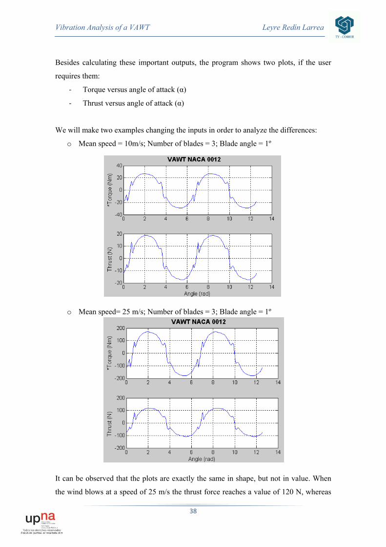
Besides calculating these important outputs, the program shows two plots, if the user
requires them:
‐ Torque versus angle of attack (α)
‐ Thrust versus angle of attack (α)
We will make two examples changing the inputs in order to analyze the differences:
o Mean speed = 10m/s; Number of blades = 3; Blade angle = 1º
o Mean speed= 25 m/s; Number of blades = 3; Blade angle = 1º
It can be observed that the plots are exactly the same in shape, but not in value. When
the wind blows at a speed of 25 m/s the thrust force reaches a value of 120 N, whereas

Vibration Analysis of a VAWT Leyre Redín Larrea
39
when the wind speed is 10m/s the thrust is about 20N. The same happens with the
Torque: for a speed of 10 m/s maximum torque is of 26 Nm, whereas for a speed of 25
m/s torque reaches the value of 160 Nm, which is considerably higher.
It is not advisable to change the number of blades because these results are just for one
blade. Meaning that in VAWT all the blades do not produce the same power because
one interferes with the others. Therefore wind speed is lower and the thrust force and
torque moment too.

Vibration Analysis of a VAWT Leyre Redín Larrea
40
6.3 GENERATOR MODEL
From all the generators that are used in wind turbines the Permanent magnet
synchronous generator (PMSG) has the highest advantages because it is stable and
secure during normal operation. Initially used only for small and medium powers the
PMSG’s are now used also for high powers.
The synchronous generator can rotate with a variable speed. If we make the rotor’s
magnet rotate it is induced an alternate current (AC) with that frequency in the stator’s
winding.
There are two types of permanent magnet synchronous generator: doubly fed and direct
drive. The second magnet is the preferred option in this case. This generator is
completely dissociated from the grid, because there is an electronic converter that
enables the system to work with variable speed [4]. This can be observed in the
following figure:
Figure 6.3.1: Scheme of a direct drive permanent magnet synchronous generator [4].
The main advantages of a variable speed wind turbines are [4]:
They generate more energy for a specific wind speed.
Active and reactive power can be easily controlled.
There is less mechanical stress.
There are few energy fluctuations due to the rotor plays the role of a flywheel.
Generally, there are not flicker problems.
The main drawback [4] of variable speed wind turbines is that power electronics is
sensitive to voltage dips caused by faults. In addition to this, these components are more
expensive than those used in asynchronous generators.

Vibration Analysis of a VAWT Leyre Redín Larrea
41
Concerning the two types of variable speed generators, it must be said that doubly fed
induction generators have an advantage versus direct drive generators, which is the size
of the generator. Direct drive PMSG is heavy and big, the electronic converter is bigger
due to the fact that 100% of the generated power has to pass through it. However, in the
doubly fed generator, just one third of this power goes through the converter. The big
advantage of direct drive PMSG is that they do not require a gearbox so their
maintenance is much lower than what doubly fed generators need [4].
Figure 6.3.2: Generator of a direct drive PMSG of a 5MW wind turbine[4]

Vibration Analysis of a VAWT Leyre Redín Larrea
42
6.4 TOWER MODEL
Two types of towers have been modeled. They are geometrically different; one is a
cylindrical tower whereas the other one is a conic tower. We will see that the conic
tower is better than the cylindrical one because it attenuates vibrations sooner. This is
because normal stresses in the base of the tower are bigger than in the top due to the
bending moment that the structure has to endure.
In a horizontal axis wind turbine the vibration happens just in one direction, so the
solution is easier as it is a one dimensional problem. Whereas in a vertical axis wind
turbine the vibration happens in both directions so the solution is more complicated. It
will be explained in the following lines how both of them have been solved by finite
element analysis.
Figure 6.4.1: Vibration in a HAWT tower on the left (one dimension) and Vibration in a
VAWT tower on the right (two dimensions).

Vibration Analysis of a VAWT Leyre Redín Larrea
43
7. VIBRATION ANALYSIS 7.1 ONE DIMENSIONAL PROBLEM
In this chapter the vibration analysis for a Horizontal axis wind turbine will be
developed. In a HAWT the vibration is just in one axis. The purpose of this chapter is to
understand the one dimensional problem in order to develop the two dimensional
problem in the following chapter.
The tower is represented as an elastic beam with mass concentrated at the top, modeling
the wind turbine:
Figure 7.1.1 Dynamical tower model [18]
The wind velocity deviation at height is set up by [18]:
V x =VL xxL
α Equation 7.1.1
Where:
‐ VL is the wind velocity at L meters height,
‐ α Hellmann exponent
‐ xL the height of the earth area (x=L), at which is accepted that the wind velocity is
zero.
The wind load acting on the rotor and the blades is represented as a concentrated force
at the free end which is determined by this equation:
F t = 12ρaπR2Cp λ, β V2 Equation 7.1.2
( )ThrustF t
f(x,t)
mg
TowerL
R
Vibration Analysis of a VAWT Leyre Redín Larrea
44
where is the tip-speed ratio, V is the wind speed, ρa is the air density, β is the blade
pitch angle and CP is power coefficient of the rotor which is determined from
experiment.
The axial load upon the turbine is taken as Thrust force (T). Distributed load upon the
height of the tower f(x,t):
f x,t = 12
ρV2 x,t D x Equation 7.1.3
Where:
‐ D(x) is the current diameter of the tower,
‐ kL correction coefficient, referring to a cylinder with limited length,
‐ CD is the drag coefficient and CL the lift coefficient
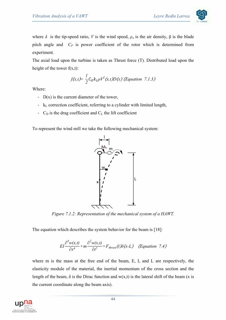
To represent the wind mill we take the following mechanical system:
Figure 7.1.2: Representation of the mechanical system of a HAWT.
The equation which describes the system behavior for the beam is [18]:
EI∂4w(x,t)∂x4 +m
∂2w(x,t)∂t2
=Fthrust t δ x-L Equation 7.4
where m is the mass at the free end of the beam, Е, I, and L are respectively, the
elasticity module of the material, the inertial momentum of the cross section and the
length of the beam, δ is the Dirac function and w(x,t) is the lateral shift of the beam (x is
the current coordinate along the beam axis).

Vibration Analysis of a VAWT Leyre Redín Larrea
45
The boundary conditions of the beam are:
- At the fixing point of the beam (х=0)
w 0,t =0 Equation 7.1.5 ; ∂w 0,t∂x
=0 Equation 7.1.6
- At the free end (x=L)
EI ∂3w(L,t)∂x3 =m1
∂w2(L,t)∂t2
Equation 7.1.7 ; ∂2w L,t∂x2 =0 Equation 7.1.8
- At the beginning, time zero:
w x,0 =0 Equation 71..9 ; w x,0 =0 Equation 7.1.10
The partial differential equation 7.4 is from fourth order and it can be written [19]:
∂2
∂x2 EI∂2w∂t2
+m∂2w∂t2
+f=0, 0<x<L, 0<t Equation 7.1.11
Where f is the external load of the system.
The FEM method for numerical solution of the system is applied in this paper [7]. The
entire area is divided at Ne elements, each consisting of 2 nodes.
One isolated element will look like:
Figure 7.1.3: One element with two nodes
The element has 4 degrees of freedom (DOF). Each node has two DOF:
1) Shift w x, t
2) Rotation: - θ = / Equation 7.1.12
The variation formation of the equation upon each element will be:
0= v ∂2
∂x2 EI∂2w∂x2 +m
∂2w∂t2
+f dx= xe+1
xe
EI∂2v∂x2
∂2w∂x2 +v m
∂2w∂t2
+f dx + v∂∂x
EI∂2w∂x2 -
∂v∂x
EI∂2w∂x2
xe
Xe+1
Equation 7.1.13xe+1
xe
θ1 θ2 u1 u2

Vibration Analysis of a VAWT Leyre Redín Larrea
46
Where v is a function differentiable 2 times on х.
Q1e=
∂∂x
EI∂2w∂x2
xe
Equation 7.1.14 Q2e=EI
∂2w∂x2
xe
Equation 7.1.15
Q3e =
∂∂x
EI∂2w∂x2
xe‐1
Equation 7.1.16 Q4e =EI
∂2w∂x2
xe‐1
Equation 7.1.17
Substituting, we obtain this expression:
0 = EI ∂2v∂x2
∂2w∂x2 + v m
∂2w∂t2
+f dx + v(xe)Q1 e
xe+1
xe
+ ∂v∂x
xe Q2e - v xe+1 Q3
e
∂v∂x
xe+1 Q4e Equation 7.1.18
The interpolation functions must fulfill the boundary conditions for both ends of the
beam:
w xe =w1, θ xe =θ1, w xe+1 =w2, θ xe+1 =θ2 Equation 7.1.19
As there are 4 conditions (4 DOF), for w we chose polynomial approximation with 4
parameters:
w x =c1+c2x+c3x2+c4x3 Equation 7.1.20
The coefficients ci are defined as functions of wi, θi in order to fulfill the conditions for
both ends of the beam:
w1 w xe c1 c2xe c3xe2 c4xe3 Equation 7.1.21
θ1 ‐∂w∂x xe ‐2c3xe‐3c4xe2 Equation 7.1.22
w2 w xe 1 c1 c2xe 1 c3xe 12 c4xe 1
3 Equation 7.1.23
θ2 ‐∂w∂x xe 1 ‐c2‐2c3xe 1‐3c4xe 1
2 Equation 7.1.24
Or matrix written:
w1θ1w2θ2
1 xe xe2 xe3
0 ‐1 ‐2xe ‐3xe2
1 xe 1 xe 12 xe 1
3
0 ‐1 ‐2xe 1 ‐3xe 12
c1c2c3c4
Equation 7.1.25

Vibration Analysis of a VAWT Leyre Redín Larrea
47
After definition of ci using w1, θ1, w2, θ2 according to the polynomial approximation
Equation 7.20 we obtain:
w x =Φ1ew1
e+Φ2eθ1
e+Φ3ew2
e+Φ4eθ2
e= ujΦje
4
j=1
Equation 7.1.26
Where
u1=w1, u2=θ1, u3=w2, u4=θ2 Equation 7.1.27
Φ1e=1-3
x-xe
he
2+2
x-xe
he
3=xe+1
3 +2x3-3xe+12 xe-3xe+1x2-3xex2+6xe+1xxe Equation 7.1.28
Φ2e=- -xe 1-
x-xe
he
2=-xe
3+xexe+12 -xxe+1
2 +x2xe+2x2xe+1-2xxexe+1 Equation 7.1.29
Φ3e=3
x-xe
he
2-2
x-xe
he
3=-xe
3+3xe2xe+1-3xxe
2-2x3+3xe+1x2+6xex2-6xe+1xxe Equation 7.1.30
Φ4e=- x-xe
x-xe
he
2-x-xe
he= xe+1xe
2-xxe2+2x2xe+x2xe+1-x3-2xxexe+1 Equation 7.1.31
As the unknown function , depends on time, it is suggested that the
approximation looks like:
we x,t = uj t Φj(x)4
j=1
(Equation 7.1.32)
Based on this approximation and functions v= i in variation from Equation 7.1.18 it
is obtained:
0= EI∂2Φi
∂x2
∂2Φj
∂x2 dxxe+1
xe
uje t +
4
j=1
mΦi x Φj(x)xe+1
xe
uj(t)+4
j=1
mΦi x fdx-Qie
xe+1
xe
(Equation 7.1.33)
or
Kije uj
(e)+ Mije uj
(e)=Fie (Equation 7.1.34)
4
j=1
4
j=1
where
Kije EI∂2Φi
∂x2∂2Φj
∂x2 dxxe 1
xe ; Mij
e mΦi x Φj xxe 1
xe; Fie ‐ mΦi x fdx Qie
xe 1
xe

Vibration Analysis of a VAWT Leyre Redín Larrea
48
In the case where , ,EI f m are constants for each element, the matrix of the elastic
coefficients [8] and the inertia matrix [8] and the general coordinates vector are
respectively:
K 2EIl3 *
6 ‐3l ‐6 ‐3l‐3l 2l2 3l l2‐6 3l 6 3l‐3l l2 3l 2l2
Equation 7.1.35 ;
M ml420
*
156 22l 54 ‐13l22l 4l2 13l ‐3l2
54 13l 156 ‐22l‐13l ‐3l ‐22l 4l2
Equation 7.1.36 ;
F ‐fl12 *
6‐l6l
Q1Q2Q3Q4
Equation 7.1.37
Based on the static equilibrium conditions of the nodes, the boundaries of two neighbor
elements, the associated coefficients are with two DOF and they can be summed, related
to element m(n-1)(n-1) it will look like simple sum. The assembled matrix M is the global
mass matrix [18]:
M * =
m11 m12 … m1(n-1) m1nm11 m22 … m2(n-1) m2n…
m(n-1)1 m(n-1)2 … m n-1 n-1 + m m n-1 nmn1 mn2 … mn(n-1) mnn
(Equation 7.1.38)
Similar structure has the global elasticity matrix , [18]:
K * =
k11 k12 … k1(n-1) k1nk21 k22 … k2(n-1) k2n
k(n-1)1 k(n-1)2 … k n-1 n-1 k n-1 n
kn1 kn2 … kn(n-1) knn
(Equation 7.1.39)

Vibration Analysis of a VAWT Leyre Redín Larrea
49
The concentrated force at the free end F(t) and the distributed load f(x,t) modify the
vector of nodal loads [18]:
F *
f x1,t *l2 f x2,t *
l2
f x1,t *l2
12 f x2,t *l2
12
f x2,t *l2 f x3,t *
l2
f x2,t *l2
12 f x3,t *l2
12…
f xn,t *l2 F t
f xn,t *l2
12
Equation 7.1.40)
Where F(t) is the external load, it has been measured for a whole rotation of the wind
turbine, each 2º. It is considered as constant data.
The assembling of the element matrices leads the problem to solve ordinary differential
equation for the unknown values {u(t)} [18]:
Equation 7.1.41)
C is the damping matrix [8]. Rayleigh damping scheme is used to form the damping
matrix as a linear combination of the mass and stiffness matrices
C =ε M +η K (Equation 7.1.42)
Where ε and η are predefined constants. The [C] coefficient has been defined
experimentally. So the predefined value for this coefficient is: C ‐0.036*K
Equation 7.1.41 results in:

Vibration Analysis of a VAWT Leyre Redín Larrea
50
f x1,t *l2
+f x2,t *l2
f x1,t *l2
12+f x2,t *
l2
12
f x2,t *l2
+f x3,t *l2
f x2,t *l2
12+f x3,t *
l2
12…
f xn,t *l2
+F t
f xn,t *l2
12
=
m11 m12 … m1(n-1) m1nm21 m22 … m2(n-1) m2n
m(n-1)1 m(n-1)2 … m n-1 n-1 +m m n-1 nmn1 mn2 … mn(n-1) mnn
*
u1u2
un-1un
+
+ε*ml420
*
156 22l 54 -13l22l 4l2 13l -3l2
54 13l 156 -22l-13l -3l -22l 4l2
*
u1u2
un-1un
+η*2EIl3
*
6 3l -6 3l3l 2l2 -3l l2
-6 -3l 6 -3l3l l2 -3l 2l2
* +
k11 k12 … k1(n-1) k1nk21 k22 … k2(n-1) k2n
k(n-1)1 k(n-1)2 … k n-1 n-1 k n-1 n
kn1 kn2 … kn(n-1) knn
Equation 7.1.43)
The application of the boundary conditions Equation 7.1.4 and 7.1.5) leads to skipping
the first two equations of the system Equation 7.43
w 0,t 0 → u1 0, u1 0, u1 0 Equation 7.1.44 ;
∂w 0,t∂x 0 θ 0,t → u2 0, u2 0, u2 0 Equation 7.1.45 .
Thus, we obtain the matrices Mnxn, Knxn and Fnx1 for the rest of the system. The
unknown vector unx1 has the following structure:
… Equation 7.1.46
For matrix exponent method application the system must be reformulated into
normalized type. Aiming this, the vector of the unknowns inside the nodes is enlarged
with n elements, which represent the first differentials with respect to the time for nodes
shifts.

Vibration Analysis of a VAWT Leyre Redín Larrea
51
0
0
0
Equation 7.1.47)
The eigenfrequencies of the tower can be obtained by solving the eigenproblem
K λ M* =0 Equation 7.1.48)
where are eigenvalues
or
u = A u + B F Equation 7.1.49)
The solution for Equation 7.49 is given by the matrix exponential using the Cauchy
formula for nonhomogenous system
Equation 7.1.50)
where t0 is the initial time.
Last expression Equation 7.50 can be discretized by using the following substitution
t0=kh t= k+1 h (k=1, 2, 3…)
Where h is the discretization step.
Approximating the integral by the Trapezium Method [21] will acquire the following
expression for the deviation values:
u k+1 h =e A h u kh +h2
e A h B F kh + B F k+1 h (Equation 7.1.51)
This solution can be used for determinate the stresses in the tower. Neglecting the Nx
internal force because it has small influence over the stresses (less than 1 MPa) and Vy
internal force due to the dimensions of the tower’s cross-section are small comparing
with its length, the following formula for calculating the stresses can be used:
σx x,t =M(x,t)
I D(x)
2 (Equation 7.1.52)
A F B

Vibration Analysis of a VAWT Leyre Redín Larrea
52
Where M(x, t) is the bending moment and D(x) is the outer diameter of the tower.
Using the known relation between bending moment and deflection:
M x,t = EI ∂2w(x,t)∂x2 (Equation 7.1.53)
Therefore, equation 7.52 acquires the following form:
σx x,t = E ∂2w(x,t)∂x2
D(x)2
(Equation 7.1.54)
7.2 TWO DIMENSIONAL PROBLEM
In this section it is described how to solve the vibration problem in two dimensions. In
vertical axis wind turbines the tower deviation is in both axes. Therefore, it is not
possible to apply the last method because the external forces acting in the wind turbine,
are correlated.
However, we finally measured the external forces experimentally, so they were not
correlated, and we used them as input data. Thereby, we carried out our Matlab program
not only following the last method, but also taking into account the forces in both axes.
The following section will describe theoretically how to solve the two dimensional
problem. However, it will not be finally carried out in Matlab.
On the one hand, a tower of a wind turbine is designed to be flexible. Therefore, the
rigid model may not be sufficient. On the other hand, flexible models with fluid forces
confined to one plane do not capture the three dimensional aspects of the problem.
Thus, in this paper, we devise a flexible model that can include the fluid forces in three
dimensions. The equations for motion are solved numerically using the finite difference
method.
Firstly, the equations of motion of the three dimensional model are derived for two
cases: rigid structure and elastic structure. The free response obtained using the rigid
model allows us to gain confidence in the formulation and the numerical results
obtained using the elastic model [22].

Vibration Analysis of a VAWT Leyre Redín Larrea
53
7.2.1 MATHEMATICAL FORMULATIONS
Rigid Model In this study, the tower is modeled as a smooth cylindrical beam, the support at the base
as a torsional spring and the structures above as a point mass.
The equations of motion when the beam is considered rigid are derived in this section.
Figure 7.2.1: Rigid beam model
From Figure 7.2.1, the system can be described with two angular degrees of freedom.
The equations of motion for a similar system were obtained in references [24, 25]. The
equations of motion are re-derived here.
The kinetic energy of the system is given by:
KE=12
{w}T I0 w +12
MP{VP}T{VP} (Equation 7.2.1)
Where is the mass moment of inertia matrix of the beam about the base, is the
point mass, and is the velocity of the point mass [22]. The first term is the kinetic
energy of the beam, and the second term is the kinetic energy of the point mass.
We consider three frames of reference, xyz, x'y'z' and xbybzb, as shown in Figure 7.2.2
xyz is the inertial reference frame, x'y'z' is obtained by rotating xyz by angle about the
x−axis. xbybzb is obtained by rotating x'y'z' by about the z' axis. xbybzb is also called
the body frame of reference since xb−axis coincides with the axis of the beam [22].
Vibration Analysis of a VAWT Leyre Redín Larrea
54
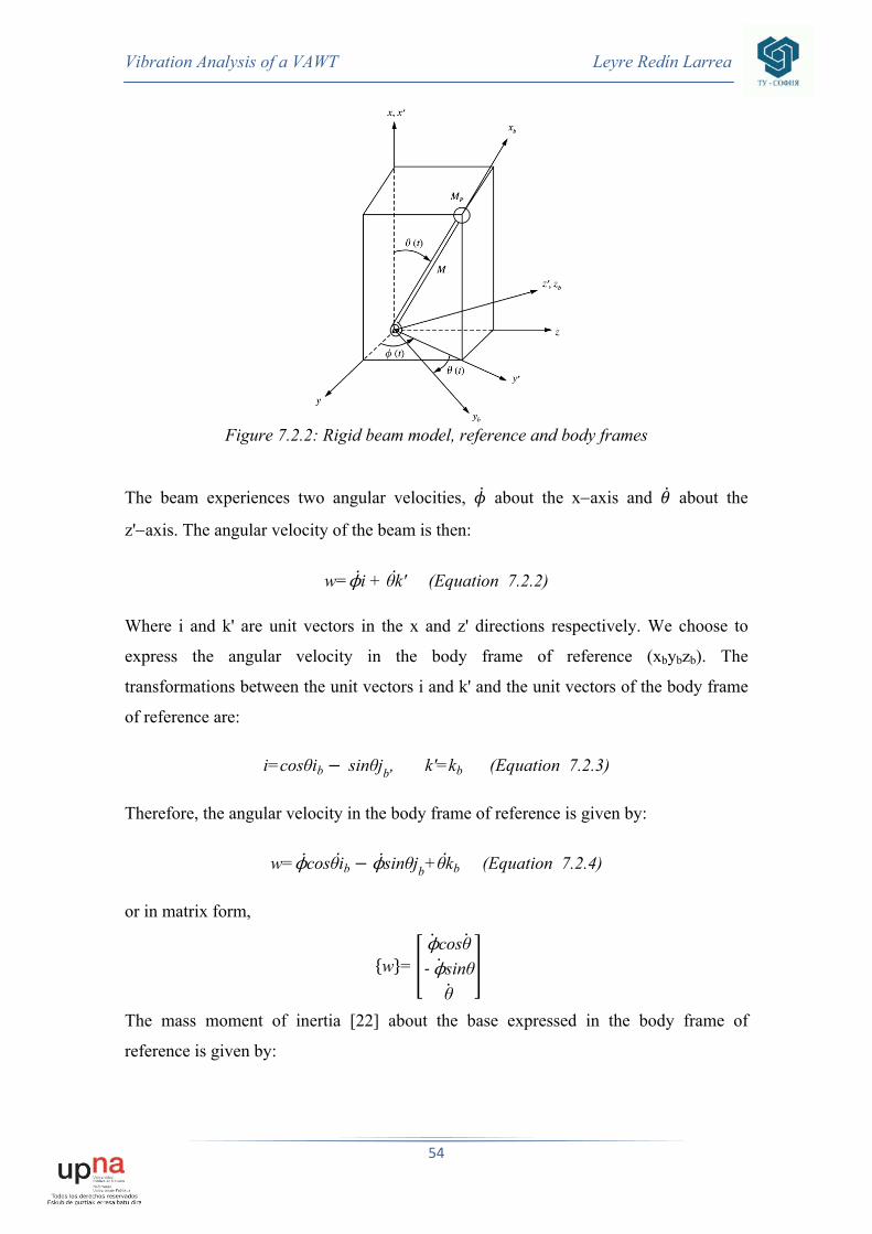
Figure 7.2.2: Rigid beam model, reference and body frames
The beam experiences two angular velocities, about the x−axis and about the
z'−axis. The angular velocity of the beam is then:
w= i + θk' (Equation 7.2.2)
Where i and k' are unit vectors in the x and z' directions respectively. We choose to
express the angular velocity in the body frame of reference (xbybzb). The
transformations between the unit vectors i and k' and the unit vectors of the body frame
of reference are:
i=cosθib sinθjb, k'=kb (Equation 7.2.3)
Therefore, the angular velocity in the body frame of reference is given by:
w= cosθib sinθjb+θkb (Equation 7.2.4)
or in matrix form,
w =cosθ
‐ sinθθ
The mass moment of inertia [22] about the base expressed in the body frame of
reference is given by:

Vibration Analysis of a VAWT Leyre Redín Larrea
55
I0
12M r02 ri2 0 0
014M r02 ri2
13ML
2 0
0 012M r02 ri2
13ML
2xbybzb
(Equation 7.2.5)
Where r0 and ri are the outer and inner radius of the beam, M is the total mass of the
beam, and L is the length of the beam. The kinetic energy of the beam is given by:
KEbeam=12
{w}T I0 w =14
M r02+ri
2 2cos2θ+12
14
M r02+ri
2 +13
ML2 2sin2θ +
12 θ
2 14
M r02+ri
2 +13
ML2 (Equation 7.2.6)
The velocity of the point mass is expressed in the inertial frame of reference [22]. First,
the displacement of the point mass is:
rp=Lcosθi + Lsinθcos j + Lsinθsin k (Equation 7.2.7)
The velocity is obtained by taking the derivative with respect to time. Since the
displacement is expressed in the inertial frame, the derivatives of the unit vectors are
zero. The velocity of the point mass is then given by:
Vp =L θsinθ
θcosθcos sinθsinθcosθsin + sinθcos xyz
(Equation 7.2.8)
The kinetic energy of the point mass is then:
KEpoint mass=12
Mp Vp T Vp = 12
MpL2(θ2sin2θ+ θcos2θcos2 - 2θ cosθcos sinθsin
+ 2sin2θsin2 + θ2cos2θsin2 + 2θ cosθsin sinθcos + 2sin2θcos2 =
12
MpL2(θ2+ 2sin2θ) (Equation 7.2.9)
Combining Equation 7.2.6 and Equation 7.2.9, the kinetic energy of the system is given
by:
KE=KEpoint mass KEbeam12
J2 θ2+ 2sin2θ +
12
J12cos2θ (Equation 7.2.10)

Vibration Analysis of a VAWT Leyre Redín Larrea
56
Where we let
J1=12
M r02+ri
2 , J2=13
ML2+MpL2+14
M r02+ri
2 Equation 7.2.11
The potential energy is stored in the torsional spring [22] and is given by:
PE=12
kθ2 Equation 7.2.12
This assumes that the structure can only bend, not twist.
The Lagrangian is the difference between the kinetic and potential energy of the system
[7], as follows:
L (Equation 7.2.13) Therefore, the Lagrangian is given by:
L=12 13
ML2 + MpL2+14
M r02+ri
2 θ2+ 2sin2θ +
14
M r02+ri
2 2cos2θ12
kθ2
(Equation 7.2.14) Lagrange's equations [7] are given by:
ddt
∂L∂qk
∂L∂qk
=Qknc , k=1,2 Equation 7.2.15
Where Qknc is the generalized non-conservative force associated with qk, and q1 and q2
are and respectively. So the equations of motion are given by:
J2 θ 2 J2 J1 2sinθcosθ + kθ =Q1 (Equation 7.2.16)
J2sin2θ 2 + 2 J2‐ J1 cos2θ 2= Q2 (Equation 7.2.17)
Elastic Model When the tower is modeled as a flexible structure, certain assumptions are made in
order to simplify the problem. In addition to the ones used in the planar Euler-Bernouilli
beam model [23], it is assumed that the rotation of the beam element can be moderate
but the strain is small [22].
In this section, the displacement field is obtained using Kirchhoff’s hypothesis, and the
corresponding strain and stress fields are obtained accordingly. The potential and kinetic
energies are then obtained to form the Lagrangian. The equations of motion are obtained
using Hamilton’s principle [7].

Vibration Analysis of a VAWT Leyre Redín Larrea
57
Displacements, strains, and stress
Using Kirchhoff’s hypothesis, the displacement field is given by:
u1=u X,t ‐ Y∂u2(X,t)∂X
‐ Z∂u3(X,t)∂X
, u2= υ X,t , u3= w X,t (Equation 7.2.18)
Where u1, u2, and u3 are displacements in x, y, and z directions respectively; u, v,
and w are the mid-plane displacements of the cross-section in the x, y, and z
directions respectively. They are also the average displacements for a symmetric
cross-section. It should be noted that the displacements are measured from the
original configuration as shown in Figure 7.2.3 [22]. The coordinates X, Y, and Z
mark the original location of a beam element (X=X, Y=0, Z=0). Note that the
average displacements are functions of X and t only.
Figure 7.2.3: Three-dimensional beam model.
The form of the displacement field implies that the shear effect is negligible when
compared to that of the bending moment. Therefore, we are assuming that the beam
is slender enough so that such an assumption is valid [22]. Also, even though it is
not obvious from the displacement field, Novozhilov [27] showed that the strains
need to be small when compared to the rotation in order for the Kirchhoff's
hypothesis to be valid. In mathematical terms,
∂u1
∂X~∂u2
∂X
2
~∂u3
∂X
2
1 (Equation 7.2.19)

Vibration Analysis of a VAWT Leyre Redín Larrea
58
The Green strain is the energy stored in a body due to its deformation [37]. The
general form of the Green strains are given by:
ε11=∂u1
∂X+
12
∂u1
∂X
2
+∂u2
∂X
2
+∂u3
∂X
2
(Equation 7.2.20)
ε22=∂u2
∂Y+
12
∂u1
∂Y
2
+∂u2
∂Y
2
+∂u3
∂Y
2
(Equation 7.2.21)
ε33=∂u1
∂Z+
12
∂u1
∂Z
2
+∂u2
∂Z
2
+∂u3
∂Z
2
(Equation 7.2.22)
ε12=12∂u2
∂X+∂u1
∂Y+∂u1
∂X∂u1
∂Y+∂u2
∂X∂u2
∂Y+∂u3
∂X∂u3
∂Y (Equation 7.2.23)
ε23=12∂u3
∂Y+∂u2
∂Z+∂u1
∂Y∂u1
∂Z+∂u2
∂Y∂u2
∂Z+∂u3
∂Y∂u3
∂Z (Equation 7.2.24)
ε13=12∂u3
∂X+∂u1
∂Z+∂u1
∂X∂u1
∂Z+∂u2
∂X∂u2
∂Z+∂u3
∂X∂u3
∂Z (Equation 7.2.25)
Using equation 7.2.19 and substituting the displacement field in
equation 7.2.18 into equations 7.2.20 to 7.2.25, the Green strains are then given by:
ε11=∂u1
∂X+
12
+∂u2
∂X
2
+∂u3
∂X
2
=u' Yv''+Zv''+12
v'2+12
w'2 (Equation 7.2.26)
ε12=ε22=ε33=ε23=ε13=0 (cross circular section) (Equation 7.2.27)
Where ' = ∂∂X and ( ) = ∂
∂t
Potential and kinetic energies
The strain energy [22] is given by:
PEstrain=12
σijεijdV0 (Equation 7.2.27)
V0
where is the second Piola−Kirchhoff stress [19]. Since is the only non−zero
strain, the strain energy is simply:
PEstrain=12
σ11ε11dA0dX (Equation 7.2.28)
A0
L
0
The stress is related to strain by the constitutive relationship [22] given by:
σij = λεkkδij + 2Gεij (Equation 7.2.29)
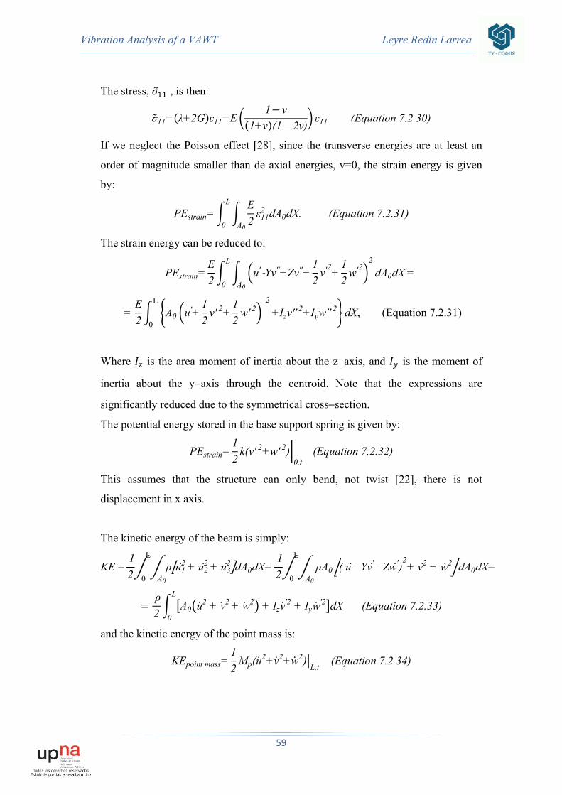
Vibration Analysis of a VAWT Leyre Redín Larrea
59
The stress, , is then:
σ11= λ+2G ε11=E1 v
1+v (1 2v)ε11 (Equation 7.2.30)
If we neglect the Poisson effect [28], since the transverse energies are at least an
order of magnitude smaller than de axial energies, v=0, the strain energy is given
by:
PEstrain=E2ε11
2 dA0dX.
A0
(Equation 7.2.31)L
0
The strain energy can be reduced to:
PEstrain=E2
u'‐Yv''+Zv''+12
v'2+12
w'22
dA0dX =
A0
L
0
= E2
A0 u'+12
v' 2+12
w' 2 2
+Izv'' 2+Iyw'' 2 dX,L
0 (Equation 7.2.31)
Where is the area moment of inertia about the z−axis, and is the moment of
inertia about the y−axis through the centroid. Note that the expressions are
significantly reduced due to the symmetrical cross−section.
The potential energy stored in the base support spring is given by:
PEstrain=12
k(v' 2+w' 2)0,t
(Equation 7.2.32)
This assumes that the structure can only bend, not twist [22], there is not
displacement in x axis.
The kinetic energy of the beam is simply:
KE = 12
ρ u1 2 + u2
2 + u32 dA0dX=
A0
L
0
12
ρA0 ( u - Yv' - Zw')2+ v2 + w2 dA0dX=
A0
L
0
ρ2
A0 u 2 + v
2 + w 2 + Izv
'2 + Iyw '2 dX
L
0(Equation 7.2.33)
and the kinetic energy of the point mass is:
KEpoint mass=12
Mp(u 2+v
2+w 2)
L,t (Equation 7.2.34)

Vibration Analysis of a VAWT Leyre Redín Larrea
60
The governing PDEs and boundary conditions using variational principles
The Lagrangian is given by:
12
′ ′
′ 12
′ 12
′ ′′ ′′
12 | ,
12
′ ′
, (Equation 7.2.35)
Let p(X,t), fy(X,t) and fz(X,t) be distributed loads in the x, y and z directions
respectively. The virtual work [7] done by these distributed loads is given by:
δW pδu fyδv fzδw dX L
0 (Equation 7.2.36)
The variation of the Lagrangian in equation 7.2.35 integrated over time is given by:
12
12
12
12
12
12
12
12
12
12
, , , , , , | 0,
12
12
| 0, (Equation 7.2.37)

Vibration Analysis of a VAWT Leyre Redín Larrea
61
Using the extended Hamilton's principle:
δ L+W dt=0, (Equation 7.2.38) tf
t0
The equations of motion are given by:
ρA0u‐ EA0 u'+12
v'2+12
v'2'
= p (Equation 7.2.39)
ρA0v- ρIzv' ' EA0 u'+12
v'2+12
w'2 v''
+ EIzv'' ''= fy (Equation 7.2.40)
ρA0w- ρIyw' '
EA0 u'+12
v'2+12
w'2 w''
+ EIyw'' '= fz (Equation 7.2.41)
and the boundary conditions are given by:
u 0,t =0, v 0,t =0, w 0,t =0 (Equation 7.2.42),
EIzv'' kv' |0,t=0, EIyw'' kw'0,t
=0 (Equation 7.2.43),
EIzv'' |L,t=0=0, EIyw'' L,t=0
, =0 (Equation 7.2.44),
EA0 u'+12
v'2+12
w'2 +MpuL,t
=0 (Equation 7.2.45),
ρIzv' EA0 u'+
12
v'2+12
w'2 v' EIzv'' '+MpvL,t
=0 (Equation 7.2.46),
ρIyw' EA0 u'+
12
v'2+12
w'2 w' EIyw'' '+Mpw
L,t=0 (Equation 7.2.47).
The boundary conditions in equations 7.2.42 indicate that displacements are zero at
X=0. Equations 7.2.43 are the moment conditions at X=0. The bending moments in
the y and z directions are proportional to the deflection of the torsional spring in
these directions. Equations 7.2.44 state that there are no bending moments at the
free end (X=L). Equation 7.2.45 expresses the fact that the normal force in the x
direction is balanced by the inertia force of the point mass in that direction.
Equations 7.2.46 and 7.2.47 indicate that the transverse shear forces are balanced
by the inertial forces of the point mass in the respective transverse directions.
Note that u(X,t), v(X,t) and w(X,t) are non−linearly coupled, and therefore, the
equations need to be solved simultaneously using numerical methods.

Vibration Analysis of a VAWT Leyre Redín Larrea
62
Linearization of equations of motion
If we further assume that the rotation squared is small when compared to the linear
strain, being rotation less than 20rad/s, the error taken is less than 5%.
∂v∂X
2 ∂u∂X 1 and
∂w∂X
2
∂u∂X 1 (Equation 7.2.48)
The Lagrangian in equation 7.2.35 becomes:
12
′ ′
′ ′′ ′′12 | ,
12
′ ′
, (Equation 7.2.49).
Then the equations of motion are given by:
ρA0u EA0 u''= p (Equation 7.2.50)
ρA0v ρIz v' '+ EIzv'' ''=fy (Equation 7.2.51)
ρA0w ρIy ''+ EIy ''
'=fz (Equation 7.2.52)
with boundary conditions:
u 0,t =0, v 0,t =0, w 0,t =0 (Equation 7.2.53),
EIzv'' -kv' |0,t=0, EIyw'' -kw'0,t
=0 (Equation 7.2.54),
EIzv'' |L,t=0=0, EIyw'' L,t=0
=0 (Equation 7.2.55),
EA0u' Mpu L,t 0 (Equation 7.2.56),
ρIzv'‐ EIzv'' ' Mpv
L,t0 (Equation 7.2.57),
ρIyw'‐ EIyw'' ' MpwL,t
0 (Equation 7.2.58).
The equations of motion are decoupled, and we recover the linear elastic equations
of motion for each direction.

Vibration Analysis of a VAWT Leyre Redín Larrea
63
7.3 VIBRATION ANALYSIS IN MATLAB As we have seen in the literature review the vibration problem has been solved using
Finite Element Analysis, the same steps have been followed. Some constants have been
predefined:
‐ Number of elements. Ne = 32.
‐ Degrees of freedom. Each node has two DOF so n=2*(Ne+1) = 66.
‐ Mass at the free end. Mm=20kg.
‐ Mass density of the tower material (steel). ρ=7850 kg/m3.
‐ Elasticity module of the tower material (steel). E=2e11.
‐ Outside diameter at the bottom of the tower. D1=0.1 m. If the tower is conic
D1=0.15m.
‐ Outside diameter at the top of the tower. D2=0.1m. If the tower is conic
D2=0.08m.
‐ Tower thickness is 0.003m.
‐ Element length. It depends on the tower length and this one is a value introduced
by the user. So element length is tower length divided by the number of
elements.
Besides this, for the analysis we have imported an exe file with the external wind
forces in axes x and y which affect the tower. They have been measured in the
laboratory for a whole rotation of the wind turbine (360º) with a step of 2º. These
forces have been read from the file and added to the distributed load at the free end
(at the top of the tower).
We apply FEA method firstly for the wind force which works in axis x and then we
repeat the FEA method but in the axis y. Thus, we obtain two plots which show the
vibrations caused by these forces and we combined both graphs.
The FEA method as explained in the previous theory consists of dividing the whole
tower in Ne elements, each one with two nodes and each node with two degrees of
freedom (shift and rotation). Therefore, we solve the problem for a single element
and we integrate for all the Ne elements.
The assembling of the element matrices leads the problem to solve ordinary
differential equation. The system is solved by matrix exponent method application
(using the Cauchy formula for nonhomogeneous system).

Vibration Analysis of a VAWT Leyre Redín Larrea
64
We obtain the expression which shows the vibration of the VAWT tower and we
plot it against time.
First of all the program asks for the input data which will be:
‐ Mean speed = 10m/s
‐ Number of blades = 3
‐ Length tower = 3 meters.
‐ Blade angle = 0
RESULTS
In the following lines I will discuss the obtained plots:
2D PLOTS
Deviation in cylindrical tower, force in axis x and y, respectively
Deviation in conical tower, force in axis x and y, respectively

Vibration Analysis of a VAWT Leyre Redín Larrea
65
The first conclusion that we can reach is that the conic tower attenuates the
vibrations in a shorter period of time than the cylindrical tower. Moreover, the first
harmonics are bigger in the cylindrical tower − 4.5*10-3 m deviation for the conical
tower whereas the cylindrical one has a deviation of 1.8*10-3 m−.
Also we can plot the stresses against time, following the equation 7.1.54.
Stresses in cylindrical tower, force in axis x and y, respectively
Stresses in conic tower, force in axis x and y, respectively

Vibration Analysis of a VAWT Leyre Redín Larrea
66
Besides, we can plot the tower deformation against the stress:
Stresses in cylindrical tower, force in axis x and y, respectively
Stresses in conic tower, force in axis x and y, respectively

Vibration Analysis of a VAWT Leyre Redín Larrea
67
It can be observed that tensions in the cylindrical tower are approximately four
times bigger than the ones in the conic tower.
Now, we will repeat some of the analysis for a wind turbine with a higher tower.
The tower is 1 meter lower than the previous one (2meters).
Stress against time of a 2 meters conic tower (force in axis x)
We can appreciate that the stress is smaller when the wind turbine tower is lower.
Vibration in a conic tower of 2 meters high

Vibration Analysis of a VAWT Leyre Redín Larrea
68
We can appreciate that the displacement of the 2m tower is slightly lower (1*10-3 m)
than the one in the 3 m tower (1.8 *10-3 m), and the vibration takes longer until it
disappears.
It is not advisable to increase the wind velocity because the plots will not change.
This does not mean that wind velocity does not interfere in the tower vibration;
indeed it is an important factor. However, the input forces have been calculated
empirically in laboratory for a mean speed of 10m/s. Therefore, we should repeat
this experiment for a different wind speed changing the input forces. This will allow
us to consider how wind speed interferes in the tower vibration.
As we have seen, the best tower is the one with conic geometry, because it absorbs
the vibrations sooner and the stress is lower than in the cylindrical tower. Now we
will compare our designed tower, which is made of steel −E=2*1011 Pa−, with a
tower made of carbon fiber −E=5,88*1011 Pa− and relative density 1940 kg/m3.
The vibrations are much smaller. The maximum deviation is less than 6*10-4 m and
they disappear quicker.
Now we repeat the analysis for a steel tower with a higher thickness, we changed it
from 3mm to 3cm.

Vibration Analysis of a VAWT Leyre Redín Larrea
69
The vibrations are much lower –the biggest deviation is 2*10-4 m–. Also, they are
attenuated sooner.
Combining these two improvements –3cm thickness and carbon fiber material
tower– the vibrations obtained for a conical tower are:
We can observe that the vibrations are absorbed in less than one second and that the
tower displacement is really small (6,5*10-5 meters).
Now we plot the maximum stress in axis X against the maximum stress in axis Y.
These maximum values happen in the base of the tower, in the foundations. We will
do this plot for the cylindrical tower and for the conic tower:

Vibration Analysis of a VAWT Leyre Redín Larrea
70
Stress in X and Y axes in a cylindrical tower of 3 meters high
Stress in X and Y axes in a conic tower of 3 meters high
3D PLOTS
Above, we plot in a 3D graph the stress in X- Y axes along the tower. So we plot the
X and Y stresses for each finite element - from Ne=1 to Ne=Ne, in our case Ne=32
elements-. Therefore, we obtain a three dimensions plot in which the axes X
represent the stress in X axis, axis Y represent the stress in this axis, and axis Z
represent the length tower, 3 meters in this case.

Vibration Analysis of a VAWT Leyre Redín Larrea
71
Stress in X and Y axes in a cylindrical during the tower’s length
Stress in X and Y axes in a conic during the tower’s length
As we can appreciate in both cases, the stress gets its maximum value in the ground,
where the foundations are. It is also observable that in the top of the tower the stress
is equal to zero. Therefore, in the top of the tower we have the maximum
deformation but the smallest stress.

Vibration Analysis of a VAWT Leyre Redín Larrea
72
Finally we plot in a 3D graph the deformation in X- Y axes along the tower. So we
plot the X and Y deformation for each finite element. Therefore, we obtain a three
dimensions plot in which the axes X represent the deformation in X axis, axis Y
represent the deformation in this axis and axis Z represent the length tower, 3 meters
in this case.
Deformation in X and Y axes in a cylindrical during the tower’s length
Deformation in X and Y axes in a conic during the tower’s length

Vibration Analysis of a VAWT Leyre Redín Larrea
73
8. COMPILING IN C++ MATLAB® is a high-level language and interactive environment for numerical
computation, visualization, and programming [29]. Using MATLAB, you can
analyze data, develop algorithms, and create models and applications. The language,
tools, and built-in math functions enable you to explore multiple approaches and
reach a solution faster than with spreadsheets or traditional programming languages,
such as C/C++ or Java™.
More than a million engineers and scientists in industry and academia use
MATLAB, the language of technical computing.
Even though Matlab is so powerful and so well known by the majority of engineers
in the world, we wanted our program to be used by everyone, not just engineers.
This is the reason why we converted the Matlab program into an exe file which can
be run in every computer in the world which has C++ compiler and Matlab
Compiler Runtime (MCR). The MCR is a standalone set of shared libraries that
enables the execution of compiled MATLAB applications or components on
computers that do not have MATLAB installed [29]. MCR can be installed in every
computer for free in a few seconds. C++ compiler is a set of compilers for C and
C++, developed by Intel. These compilers are available for Linux, Microsoft
Windows and Mac OS X so it is really easy to have it installed in your computer.
Thereby, every person in the world can use our program, no matter if it is an
engineer interested in the vertical axis wind turbine design or an economist
interested in VAWT business. Moreover, as the GUI interface is so friendly the user
does not need to understand the complex Matlab code to comprehend the analysis.
For converting the mfile to an exe file the following function has been used [29]: mcc -m GUI_leyre
This function creates an exe file called GUI_leyre which can be executed from
every computer that has C++ and MCR.

Vibration Analysis of a VAWT Leyre Redín Larrea
74
9. MEASUREMENTS AND RESULTS The last part of the thesis was focused on real measurements on the vertical axis wind
turbine. It is a three-bladed vertical axis wind turbine with a cylindrical tower of 2
meters high.
Firstly, we had to take the VAWT to the roof and fix it to the ground to make sure that it
behaved like a beam with a fix end.
Figure 9.1 Vertical axis wind turbine prototype in the laboratory
An important task was to measure the wind turbine rotation speed. We did it with a
digital tachometer: UNI-T UT372. It has a range from 10rpm to 99999rpm. The speed
was more or less constant, between 40 and 60 rpm.
Figure 9.2: Digital tachometer UNI-UT372

Vibration Analysis of a VAWT Leyre Redín Larrea
75
After this, we prepared all the equipment. We used the CompactDAQ – 9174 National
Instrument device [35], a very accurate system. Its data sheet is in annex 1. The
software used for data acquisition was LabVIEW Signal Express. It is an interactive
data-logging software for quickly acquiring, analyzing, and presenting data from, with
no programming required.
Figure 9.3: National instrument device
The device has four sensors, which are accelerometers for measuring the tower
vibrations. An accelerometer is a device that measures the vibration, or acceleration of
motion of a structure [36]. The force caused by vibration or a change in motion –
acceleration– causes the mass to squeeze the piezoelectric material, which produces an
electrical charge that is proportional to the force exerted upon it. Since the charge is
proportional to the force, and the mass is a constant; then the charge is also proportional
to the acceleration. The accelerometer’s data sheet is in annex 2.
Once they were connected to the computer we placed them in our VAWT. We were
interested in analyzing the vibrations in different parts of the VAWT:
‐ Generator (it is situated in the top of the tower)
‐ Tower
o Top of the tower
o Middle of the tower
o Bottom of the tower.
The accelerometers are directional, meaning that they can only measure in one axis. For
measuring in three dimensions we would need multi-axes accelerometers. As we were
only interested in measuring the vibrations in the tower they were not needed.
Accelerometer

Vibration Analysis of a VAWT Leyre Redín Larrea
76
For some of the measures we used three of the accelerometers, separated 120º between
them. Moreover, we repeated the measures with only two sensors, placing them with
90º between them.
After locating the devices in our VAWT, we started the software. Firstly, we set up the
following values, which are the default ones.
Figure 9.4: Set up values for initializing the software
After making some changes in the properties such as colours or the number of plots, we
were ready for the data acquisition. We clicked on the run bottom and waited for the
plots. After having all the data, we exported it in a excel file for further analysis.
Figure 9.5: Plots of the responses of the four devices. They are so sensitive that the noise disturbs the signal.

Vibration Analysis of a VAWT Leyre Redín Larrea
77
Firstly, we needed to apply some filters in order to have an undisturbed signal, without
noise. As the accelerometers measures in milivolts, we had to turn them into meters per
second squared, by taking into account the Earth acceleration as well. This was done
multiplying the data with the passport graph from the accelerometer data and taking a
correction coefficient depending on the Earth’s position. Besides, as we were looking
for displacement of the tower we had to integrate this data two times.
The resulting plot shows the tower’s deviation -in meters- against time -in seconds-:
Figure 9.6: Vibrations response in the VAWT prototype. It shows deviation against time

Vibration Analysis of a VAWT Leyre Redín Larrea
78
10. CONCLUSIONS COMPARISON MEASUREMENTS AND MATLAB RESULTS
Figure 10.1: Comparison vibrations in VAWT prototype with the ones obtained modeling in Matlab
As it can be observed, both responses are quite similar. The maximum deviation in the
real VAWT prototype is a little bit smaller than 1 mm, whereas in our Matlab program
the displacement is 1mm. This small difference might be due to experimental error. In
the laboratory there are many factors that disturb the data and this is why the response is
slightly different.
Moreover, it can be seen that the vibration frequency is almost the same.
Furthermore, it can be appreciated that the damping is almost equal. Actually, in both
cases the vibration is absorbed in 18 seconds.
We can conclude that our Matlab model has been successfully validated, as the results
are very close to the ones obtained in the VAWT prototype, despite experimental errors.
Therefore, our Matlab program is a reliable software for analyzing vibrations in a
Vertical Axis Wind Turbine tower.

Vibration Analysis of a VAWT Leyre Redín Larrea
79
IMPROVEMENTS THAT COULD OPTIMIZE THE DESIGN OF A WIND TURBINE TOWER:
As we have proved, the maximum stress happens in the base of the tower.
Therefore, a good idea would be to build a tower with a variable thickness, wider at
the base and, as we move up along the tower height, the thickness gradually
decreases. This way we will optimize the cost of the tower, because in the top part of
it the stress is very small so we do not need so much material.
The geometry of the tower should be conic instead of cylindrical because the
stress in the tower is weaker. The vibrations are attenuated sooner and the biggest
deformation is smaller. As we have tested in the program:
Figure 10.2 Vibrations in a cylindrical and conic tower, respectively
Figure 10.3 Stress in X and Y, along the tower height, for cylindrical and conic
tower, respectively

Vibration Analysis of a VAWT Leyre Redín Larrea
80
Tower oscillations can be reduced if the tower modal damping increases;
what would require change in tower structural parameters, such as mass and stiffness
distributions.
Using a better material for the tower; such as a composite material, for
instance, fiberglass or carbon fiber. Its Young module is higher, so they are more
resistant to vibrations. We checked this with our Matlab program, for the carbon
fiber tower the highest deformation was of 0.6 mm, whereas in the steel tower it is of
1.8 mm. Moreover, in the first one the vibration is attenuated in ten seconds, but in
the other one it needs more than 20 seconds to disappear. The results were:
Figure 10.3: Vibrations in a carbon fiber conic tower and a steel tower,
respectively.
Increasing the thickness of the whole tower will reduce the tower vibrations.
We checked this with our Matlab program, when the tower thickness is 3cm the
maximum deformation is 0.2mm, whereas when the thickness is 3mm, the maximum
deformation is 1.8mm. Moreover, in the first one the vibration is attenuated in about
five seconds but in the other one it needs more than 20 seconds to disappear and the
result is:

Vibration Analysis of a VAWT Leyre Redín Larrea
81
Figure 10.4: Vibrations in a 3cm thickness conic tower and a 4cm thickness
tower, respectively.
The first improvement must be taken into account when designing a wind turbine
tower, because it reduces the tower vibrations as well as making the tower more cost
efficient. Moreover, choosing a conic tower decreases the stress, vibrations and
tower cost because it requires less material for building it, as in the top of the tower
the diameter is smaller.
However, the last two improvements might not optimize the tower’s design because,
although it reduces the stress, they are expensive measures. Thereby, for small wind
turbines they might be unworthy. On the other hand, if we want to design a bigger
wind turbine, these improvements must be taken into account.
Therefore, the tower design should be a conic tower with variable thickness.
FUTURE WORK: ‐ It would be a great idea to model the tower in another powerful program for
finite elements, such as Abaqus, Ansys or Marc. This way, we will be able to
compare our Matlab designed program with a different software.
‐ An interesting idea would be to implement this model for offshore applications.
As we already explained, this wind turbine has many advantages for offshore
due to its low weight. For this task, we should take into account the wave power
apart from the wind power. Nowadays, research regarding this topic is still
ongoing. However, in the near future, offshore wind turbines will be at least as
important as inshore ones.

Vibration Analysis of a VAWT Leyre Redín Larrea
82
11. ANNEXES ANNEX 1: UNI-T UT372 Digital Tachometer Sheet Data
The digital tachometer measures rotation speed within 10-99999 range.
UNI-T UT372 Digital Tachometer Features
• Range: 10-99999 • Data Hold function • Max/Min/Ave/Zero measurements • Sleep mode • Low battery indication •
UNI-T UT372 Digital Tachometer Technical Specifications
Display LCD, 99999, 53 × 41mm
Range, RPM
10 to 99 100 to 999
1000 to 9999 10000 to 99999
Best accuracy 0.04% ± 2dgt
Target distance, mm 50 to 200 mm
Power 1.5V Battery (AA) × 4
Dimensions (H × W × D), mm 184 × 56 × 34
Weight, g 100

Vibration Analysis of a VAWT Leyre Redín Larrea
83
ANNEX 2: Compact DAQ-9174 National Instruments data sheet [36]
Technical Sales Bulgaria +359 2 979 77 55 [email protected]
NI cDAQ-9174
NI CompactDAQ 4-Slot USB Chassis
• Choose from more than 50 hot-swappable I/O modules with integrated signal conditioning • Access the 4 general-purpose 32-bit counter/timers built into the chassis through the digital module • Run 7 hardware-timed operations simultaneously from analog, digital, or counter/timer channels • Stream continuous waveform measurements with patented NI Signal Streaming technology • Take advantage of Windows 7 OS support • Measure in minutes with NI-DAQmx software and automatic code generation using the DAQ Assistant
Overview
The NI cDAQ-9174 is a 4-slot NI CompactDAQ USB chassis designed for small, portable, mixed-measurement test systems. Combine the cDAQ-9174 with up to four NI C Series I/O modules for a custom analog input, analog output, digital I/O, and counter/timer measurement system. Modules are available for a variety of sensor measurements including thermocouples, RTDs, strain gages, load and pressure transducers, torque cells, accelerometers, flow meters, and microphones. NI CompactDAQ systems combine sensor measurements with voltage, current, and digital signals to create custom, mixed-measurement systems with a single, simple USB cable back to the PC, laptop, or netbook. The cDAQ-9174 has four 32-bit general-purpose counter/timers built in. You can access these counters through an installed, hardware-timed digital NI C Series module such as the NI 9401 or NI 9402 for applications that involve quadrature encoders, PWM, event counting, pulse train generation, and period or frequency measurement. The cDAQ-9174 chassis is shipped with the following: - AC/DC converter that plugs directly into the chassis - USB cable with a thumbscrew lock for strain relief Power cord sold separately. For conditions where EMI could be an issue, you can use the 7.0 mm EMI suppression ferrites to suppress EMI for BNC cabling to the chassis.

Vibration Analysis of a VAWT Leyre Redín Larrea
84
NI-DAQmx driver software is shipped with every chassis and includes the following: - LabVIEW SignalExpress LE for simple data-logging applications - API for LabVIEW, ANSI C/C++, C#, and Visual Basic .NET - DAQ Assistant code generation for NI LabVIEW, LabWindows™/CVI, and Measurement Studio - Example programs for all supported languages - NI Measurement & Automation Explorer (MAX) for system configuration and test The mark LabWindows is used under a license from Microsoft Corporation. Windows is a registered trademark of Microsoft Corporation in the United States and other countries.
Specifications
General
Product Name cDAQ-9174
Form Factor USB , CompactDAQ
Product Type Chassis
Part Number 781157-01
Operating System/Target Real-Time , Windows
LabVIEW RT Support No
Operating Relative Humidity 10 percent , 90 percent
Chassis
Number of Slots 4
Total Available Power 15 W
Input Voltage Range 9 V , 30 V
Built-In Trigger No
Counter/Timers
Counters 4
Resolution 32 bits
Bus Interface
USB Specification USB 2.0 Hi-Speed
High-Performance Data Streams 7
Types Available Digital Output , Counter/Timer Input , Digital Input , Analog Output , Analog Input
Shock and Vibration
Operational Shock 30 g
Random Operating Frequency Range 5 Hz , 500 Hz

Vibration Analysis of a VAWT Leyre Redín Larrea
85
General
Random Vibration 0.3 g
Physical Specifications
Length 15.9 cm
Width 8.81 cm
Height 5.89 cm
Weight 574 gram
Minimum Operating Temperature -20 °C
Maximum Operating Temperature 55 °C
Maximum Altitude 5000 m

Vibration Analysis of a VAWT Leyre Redín Larrea
86
ANNEX 3: Accelerometer KD35
Kennblatt für Schwingungsaufnehmer
Clibraton Chart for Accelerometer Typ KD 35. Nr. 82329
Individual characteristics:
Voltage Sensitivity BUA (125 Hz) = 5,00 mv/ms-2
Setprint 1/ BUA = 0,20 ms-2/mV
Charge Sensitivity
Capacitance with 1,5 m cable Ci+CK = 0,89 nF
Cable capacitance CK (1,5 m) = 0,15 nF. CK (5 m) = 0,50 nF
Resonance frequency (Bonding to steel mass of 200g) FR s.Diagramm kHz
Cross-axis sensitivity Γ90max = 3,6%
Insulation resistance Ris > 1000 MΩ
Date: 2. 9. 2011
We give a guarantee for this accelerometer in the lawful wextent for the time of 24 months after bargain

Vibration Analysis of a VAWT Leyre Redín Larrea
87
12. REFERENCES [1] Paul Deglaire. Analytical Aerodynamic Simulation Tools for Vertical Axis Wind
Turbines. Thesis (doctor in engineering). Sweden, Uppsala University, November
2010.
[2] Justin Wilkes, Jacopo Moccia and Mihaela Dragan. Wind in Power, 2011
European statistics. The European Wind Energy Association (EWEA), February
2012.
[3] Ben Backwell. Bulgaria wind power capacity to reach to 3GW by 2020. Recharge
journal, wind section [online]. November 2009, updated December 2012.
Available in:
http://www.rechargenews.com/news/policy_market/article1282510.ece
[4] Joseba Ripa Professor. Wind turbine types. Energy Technology. Public University
of Navarra. October 2011.
[5] Marco D’Ambrosio and Marco Medaglia.Vertical axis wind turbines: History,
technology and applications. Thesis (doctor in energy engineering). Sweden,
Högskolan University, May 2010.
[6] Floating Offshore Wind Project INFLOW Kicks-Off in France. Offshore Wind
News Turbine magazine [online]. 6 September 2012. Available online in
http://www.offshorewind.biz/2012/09/06/floating-offshore-wind-project-inflow-
kicks-off-in-france/
[7] Jose Manuel Jimenez Bascones Professor. Vibration introduction (Chapter 1).
Vibrations and machine elements. Public University of Navarra. February 2010.
[8] Jose Manuel Jimenez Bascones Professor. Vibration notions and definitions
(Chapter 2). Vibrations and machine elements. Public University of Navarra.
February 2010.
[9] M. E. H. Benbouzid, D. Diallo, Y. Amirat, H. Mangel and A. Mamoune
Development of Wind Turbines Prototyping Software. In: International
Conference on Electrical Machines (2006, Chania, Greece). Electrical and
Computer Engineering Professional Institute (IUP GEII) in Amiens, France.
[10] Joseba Ripa Professor. Wind characteristics. Energy Technology. Public
University of Navarra. October 2011.
Vibration Analysis of a VAWT Leyre Redín Larrea
88
[11] Pedro Rosas. Dynamic influences of wind power on the power system. PhD
Thesis. Orsted Istitute (Section of Electric Power Engineering). Technical
University of Denmark. March 2003.
[12] Jianhui Zhang. Numerical Modeling of Vertical Axis Wind Turbine. Master thesis.
Technical University of Denmark (Department of Mechanical Engineering),
December 2004.
[13] M.C. Claessens. The design and testing of airfoils for application in small vertical
axis wind turbines. Science Thesis. Holland, Delf University of Technology,
Faculty of Aerospace Engineering. October 2006.
[14] Joseba Ripa Professor. Wind turbine aerodynamics. Energy Technology. Public
University of Navarra. October 2011.
[15] Habtamu Beri, Yingxue Yao. Double multiple stream tube model and numerical
analysis of vertical axis wind turbine. Energy and Power Engineering journal
[online].Vol.3, No. 3, July 2011, pp. 262-270. Available in:
http://www.SciRP.org/journal/epe
[16] Wind Turbine Control Toolbox manual. Princeton Satellite Systems. New Jersey,
January 2009.
[17] C. Ghiţă, A.-I. Chirilă, I.-D. Deaconu and D.-I. Ilina. Wind turbine permanent
magnet synchronous generator magnetic field study. Romania, Polytechnic
University of Bucharest, Department of Electrical Engineering. 2006.
[18] Julian Genov, Gancho Venkov, Bogdan Gilev. Modeling and control of horizontal
axis wind turbine (part1 dynamical model and linearization). Mechanics
Department, Technical University of Sofia. 2012.
[19] Singiresu S. Rao. Vibration of continuous systems. University of Miami,
published by John Wiley&Sons, New Jersey, 2007, pp 344-350
[20] S. Timoshenko. Vibration problems in engineering. Second edition, New York, d.
Van Nostrand Company publisher, 1937.
[21] Autar Kaw, Charlie Barker. Trapezoidal Rule. Holistic Numerical Methods
Institute. University of South Florida.
[22] Han and H. Benaroya. Vibration of a compliant tower in three-dimensions.
Journal of Sound and Vibration. Vol. 250 No. 4, pp 675-709. Department of
Mechanical and Aerospace Engineering, Rutgers, the State University of New
Jersey, U.S.A, 2002.

Vibration Analysis of a VAWT Leyre Redín Larrea
89
[23] O.A. Bauchao and J.I. Craig. Solid Mechanics and its Applications. Georgia
Institute of Technology, Atlanta, U.S.A. Springer publisher, New York, pp 174-
176
[24] R. K. Jain and C.L. Kirk. Dynamic response of a double articulated offshore
loading structure to noncollinear waves and current. Journal of Energy Resources
Technology 103. England, 1981, pp 41-47.
[25] P. Bar-Avi and H. Benaroya. Nonlinear Dynamics of Compliant Offshore
Structures. Lisse, The Netherlands. Swets and Zeitlinger Publishers, 1999.
[26] A. E. H. Love. On the small free vibrations and deformations of elastic shells.
Philosophical trans. of the Royal Society (London), 1888, Vol. serie A, No. 17 pp.
491–549.
[27] G. L. Baker and J. P. Gollub. Chaotic Dynamics, an Introduction. Cambridge,
U.K. Cambridge University Press editor, 1996.
[28] L. Ortiz Berrocal, Elasticidad, McGraw-Hill, 1998
[29] Rafic Bachnak and Roger Lee. Converting m-files to Stand-Alone applications.
The Electronic Journal of Engineering Technology, Vol 5 No.1, winter 2003.
Texas A&M University
[30] Matlab online website: http://www.mathworks.es
[31] MATLAB video. Building Project MainApp, Matlab Compiler. 3:15 minutes.
Available online in www.mathworks.es
[32] MATLAB video. Creating a GUI with GUIDE. 10:29 minutes. Available online
in www.mathworks.es.
[33] MATLAB. Creating Graphical User Interfaces. Natick Massachusetts, United
States. March 2013. Available online in www.mathworks.es
[34] Matlab R2012b Help. Natick Massachusetts, United States ,2012.
[35] CompactDAQ – 9174 National instruments device data sheet. Available online in
National Instruments web page: http: www.see.ni.com
[36] Introduction to accelerometers. Available online in OMEGA Engineering
Technical Reference web page: http: www.omega.com
[37] Stress and Strain Tensors – Deformation and Strain. MCEN 5023/ASEN 5012.
Chapter 4. Fall, 2006.