vibration of bandsaws
TRANSCRIPT

VIBRATION OF BANDSAWS
A THESIS
SUBMITTED IN PARTIAL FULFILMENT
OF THE REQUIREMENTS FOR THE DEGREE
OF
DOCTOR OF PHILOSOPHY IN MECHANICAL ENGINEERING
IN THE
UNIVERSITY OF CANTERBURY
by
Lan Lengoc
University of Canterbury
1990

Me'n t~ng Thu H&ng

bact
The aim of this thesis was to investigate the vibrational characteristics of wide band
bandsaws.
Firstly, the vibration of bandsaw structures was considered.
A computer program was developed to predict the natural frequencies and mode
shapes of three dimensional structures, consisting of beams, springs, viscous dampers,
concentrated masses, and gyroscopic rotors. The method used was the dynamic stiff
ness method.
Some of the vibrational characteristics of the bandsaw structure were then estab
lished from experimental results and results obtained from the computer program.
The gyroscopic effects on the bandsaw structure due to rotating pulleys were also
examined.
Secondly, the dynamic stiffness method was used to solve the moving beam prob
lem. The moving beam had been used previously to model the bandsaw blade. The
dynamic stiffness method allowed complex problems to be analysed in a systematic
manner.
A moving beam proved to be too crude a representation of a wide bandsaw blade
at the level of detail being investigated. Therefore, attempts were made to model
the dynamic behaviour of wide bandsaw blades with moving plates.
A general approach to the solution of the moving plate problem is presented in

11
this thesis, it uses the extended Galerkin method to discretise the partial differential
equation of motion and the boundary conditions into a quadratic eigenvalue problem.
The solutions for this problem were obtained by using a linearisation technique.
The effects of in~plane stresses on bandsaw blades are considered in this thesis.
Three cases are examined; a linearly distributed stress across the width of the blade
due to wheel~tilting and/or backcrowning, a parabolic distributed stress across the
width of the blade due to prestressing, and stresses induced by tangential cutting
forces.
Parametric instabilities due to fluctuating tension, and due to periodic tangential
cutting forces were investigated. The harmonic balance method was used on the
discretised form of the moving plate equation to obtain the required instability
regIOns.
Finally, the dynamic instability of a moving plate due to a nonconservative com
ponent of the tangential cutting force was considered. The method of solving this
nonconservative problem was the same as that used to solve the conservative case.

e
1 INTRODUCTION
1.1 Historical Background
1.1.1 Structural Vibrations.
1.1.2 Dynamics of Bandsaw Blades
1.1.3 Dynamics of Plates
1.2 Scope of the Project ...
2 THE DESIGN OF A TYPICAL BANDSAW
2.1 General Assembly ....
2.2 Section Below the Base .
2.3 Section Above the Base.
2.4 Straining Device.
2.5 Saw Blade . . . .
1
2
3
4
8
10
11
11
12
16
19
22
3 EXPERIMENTAL METHOD IN STRUCTURAL VIBRATIONS 27
3.1 Introduction..................
3.2 General Procedure in Experimental Analysis
3.2.1 Excitation of the Structure ..... .
3.2.2 Measurement of the Vibrations and the Excitations
3.2.3 Analysis ....................... .
11l
27
28
28
29
30

CONTENTS
3.3 Instrumentation ....... .
3.3.1 Methods of Excitation
3.3.2 Vibration Measurement Techniques
3.3.3 FFT Analyser . . . . . . . . . . . .
IV
31
31
32
34
4 THEORETICAL METHOD IN STRUCTURAL VIBRATIONS 35
4.1 Modelling the Bandsaw Structure 35
4.2 Methods of Analysis ....... 36
4.3 A General Procedure in the Dynamic Stiffness Method 37
4.4 Dynamic Stiffness Matrices. . . . . . . . . .
4.4.1
4.4.2
4.4.3
4.4.4
4.4.5
4.4.6
4.4.7
Transverse Vibration of Thin Beams
Transverse Vibration of Thick Beams
Longitudinal and Torsional Vibration of Beams
3D Beam Elements .
Concentrated Masses
Gyroscopic Rotors
Springs ..
4.4.8 Dampers.
4.5 Problem with the Infinite Magnitude of the Determinants.
4.6 Coordinates System and Transformations.
4.6.1 Coordinates System ...... .
4.6.2 Transformation of Coordinates.
4.6.3 Assemblying the Global Stiffness Matrix
4.7 Roots Finding Method . . . . . . . . .
4.8 Description of the Computer Program
4.8.1 Hierarchical Structure of VIB3 .
4.8.2 Input Data .......... .
38
38
41
42
44
45
46
47
48
49
50
51
52
55
55
58
58
59
CONTENTS v
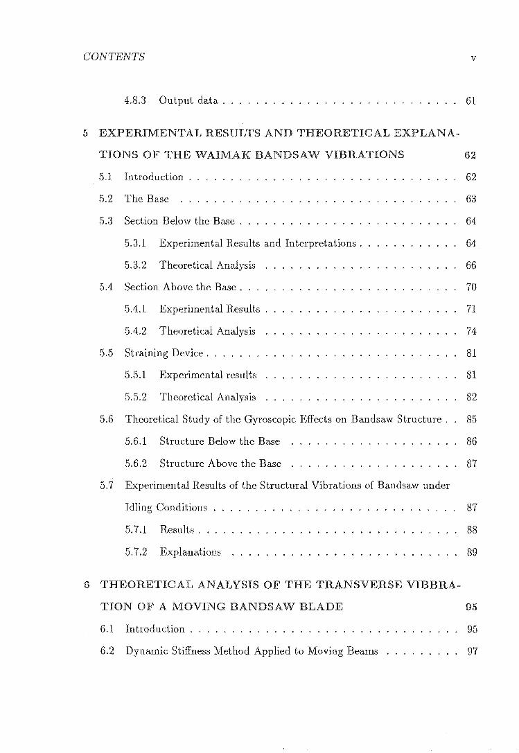
4.8.3 Output data. . . . . . . . . . . . . . . . . . . . . . . . . . . . 61
5 EXPERIMENTAL RESULTS AND THEORETICAL
TIONS THE WAIMAK BANDSAW VIBRATIONS
5.1 Introduction.
62
62
5.2 The Base .. 63
5.3 Section Below the Base . 64
5.3.1 Experimental Results and Interpretations. 64
5.3.2 Theoretical Analysis 66
5.4 Section Above the Base. . . 70
5.4.1 Experimental Results. 71
5.4.2 Theoretical Analysis 74
5.5 Straining Device. . . . . . . 81
5.5.1 Experimental results 81
5.5.2 Theoretical Analysis 82
5.6 Theoretical Study of the Gyroscopic Effects on Bandsaw Structure. 85
5.6.1 Structure Below the Base 86
5.6.2 Structure Above the Base 87
5.7 Experimental Results of the Structural Vibrations of Bandsaw under
Idling Conditions . . . . . . . . . . . . . . . . . . . . . . . . . . . .. 87
5.7.1 Results.... 88
5.7.2 Explanations
6 THEORETICAL ANALYSIS OF THE TRANSVERSE VIBBRA-
TION OF MOVING BANDSAW BLADE
6.1 Introduction .................. .
6.2 Dynamic Stiffness Method Applied to Moving Beams
89
95
95
97

CONTENTS
6.3 Effects of Boundary Conditions on a High Strain Moving Beam
6.3.1 Varying Length .
6.3.2 Varying Tension.
6.3.3 Varying Axial Speed
6.3.4 Conclusion ...
6.4 Multiple Span Beams.
6.4.1 Three Equal Span Lengths .
6.4.2 Long Centre Span.
6.4.3 Short Centre Span
6.4.4 Conclusion.....
6.5 Boundary Excitation of Moving Beams
VI
· 101
· 102
· 103
· 105
· 106
· 106
· 107
· 109
· 113
· 113
· 113
7 A GENERAL PROCEDURE IN
RECTANGULAR PLATE
DYNAMIC ANALYSIS OF
117
7.1 Introduction ....... .
7.2 Formulation Hamilton's Principle
7.2.1 Hamilton's Principle ....
7.2.2 Kinetic and Potential Energy of a Plate.
· 117
· 118
· 119
· 120
7.2.3 Calculus of Variations .......... . 121
7.2.4 Equation of Motion and Boundary Conditions . 123
7.3 Exact Solutions for Plates with Simple Boundary Conditions . 124
7.3.1 SS-SS-SS-SS Plates . . . . . . . 126
7.3.2 SS-F-SS-F Rectangular Plates . 126
7.4 Approximate Solutions - Galerkin Method
7.4.1 Methods of Approximation.
7.4.2 Galerkin Method ..... .
7.5 Plate Solutions Using Galerkin Method
· 129
· 129
· 131
· 133

CONTENTS VB
7.5.1 Discretisation of the Plate Equation. · 133
7.5.2 SS-SS-SS-SS Plates . . . . . . . . · 135
7.6 Trial Functions for the SS-F -SS-F Plate . · 136
7.7 Extended Galerkin Method for SS-F-SS-F Plates. · 139
7.7.1 Extended Weighted Residual Method · 140
7.7.2 Weak Form of the Plate Equation · 141
7.7.3 SS-F-SS-F Plates ....... " · 141
7.8 A Computer-Oriented Procedure · 143
7.8.1 Eigenvalue Solver - PC-MATLAB · 143
7.8.2 Numerical Integration ..... ., · 144
7.8.3 Computer Language - The C Language · 144
7.8.4 The Procedure ........ '" '" .... · 145
7.9 Numerical Integration - Gaussian Quadrature · 147
8 MOVING PLATES 149
8.1 Introduction ... · 149
8.2 The Formulation · 150
8.3 Approximate Solutions for a Moving SS-F-SS-F Plate · 153
8.3.1 Galerkin Equation . . ~ .. . .. . · 153
8.3.2 Quadratic Eigenvalue Problems · 155
9 STRESSES IN BANDSAW BLADES 157
9.1 Introduction . . . . . . . . . . . . . . . · 157
9.2 General Formulation and Method of Solutions · 158
9.2.1 Formulation . . . . . · 158
9.2.2 Method of Solutions · 160
9.3 Stresses due to the Static Tension · 162

CONTENTS
9.3.1 Stress Characteristics ..... .
9.3.2 Stationary Plates under Tension.
9.3.3 Moving Plate under Tension
9.4 Stresses due to Wheel-tilting and Back-crowning.
9.4.1 Stress Characteristics.
9.4.2 Wheel-tilting
9.4.3 Back-crowning.
9.5 Stresses due to Prestressing
9.5.1 Stress Characteristics.
9.5.2 Kirbach and Bonae Experimental Results.
9.5.3 Tanaka et.a1. Experimental Results
9.5.4 Conclusion...... ..
9.6 Stresses Induced by Cutting Forces
9.6.1 Cutting Forces ..
9.6.2 Stress Characteristics .
9.6.3 Magnitude of Cutting Forces.
9.6.4 Results for a Stationary Blade.
9.6.5 Results for a Moving Blade
9.6.6 Conclusion ........ .
Vlll
· 162
· 163
· 164
· 166
· 166
· 168
· 172
· 175
· 176
· 182
· 183
· 185
· 185
· 186
· 188
· 190
· 190
· 193
· 193
10 STABILITY OF BANDSAW BLADE UNDER PARAMETRIC
EXCITATIONS 196
10.1 Introduction . · 196
10.2 Method of Analysis · 197
10.2.1 Introduction . · 197
10.2.2 Harmonic Balance Method · 199
10.3 Periodic Tension Fluctuation ... .204

CONTENTS IX
10.3.1 Stationary Blades . .204
10.3.2 Moving Blade · 207
10.4 Periodic Tangential Cutting Forces .211
10.4.1 Stationary Blades · 212
10.4.2 Moving Blades · 214
11 STABILITY OF BANDSAW BLADES UNDER NONCONSER-
VATIVE CUTTING FORCES
11.1 Nonconservative Problems ..
11.2 Nonconservative Cutting Forces on Bandsaw Blades
11.3 Formulation of Nonconservative Problems
11.4 Method of Analysis ..
11.5 Results and Discussion
11.5.1 Stationary Blades
11.5.2 Moving Blades
12 CONCLUSION
12.1 Summary ..
217
.217
.222
.224
.225
.228
· 228
.230
234
· 234
12.1.1 Analysis of Structural Vibrations . 234
12.1.2 Structural Vibration of the Waimak Bandsaw . 235
12.1.3 Boundary Conditions of Moving Bandsaw Blades . 236
12.1.4 Analysis of Plate . . . . . . 237
12.1.5 Stresses in Bandsaw Blade . 238
12.1.6 Parametric Excitations on Bandsaw Blades. . 239
12.1.7 Nonconservative Cutting Forces on Bandsaw Blades. . 240
12.2 Future Work. . . . . . . . . . . . . . . 241
12.2.1 Mechanism of Cutting Wood. . 241
CONTENTS x
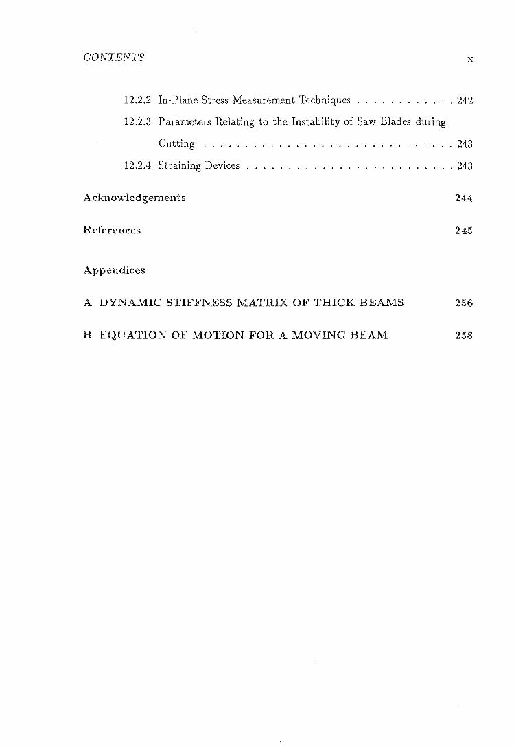
12.2.2 In-Plane Stress Measurement Techniques ............ 242
12.2.3 Parameters Relating to the Instability of Saw Blades during
Cutting . . . . . . . . . . . . . . . . . . . . . . . . . . . . . . 243
12.2.4 Straining Devices . . . . . . . . . . . . . . . . . . . . . . . . . 243
Acknowledgements 244
References 245
Appendices
A DYNAMIC STIFFNESS MATRIX OF THICK BEAMS 256
EQUATION OF MOTION FOR A MOVING BEAM 258

* 1
1 First two natural frequencies of a stationary blade with simply-supported
and clamped-clamped end conditions.. . . . . . . . . . . . . . . 102
2
3
First two natural frequencies of a blade with different tensions ..
First two natural frequencies of a blade with various axial speeds.
4 First two natural frequencies of the Waimak saw blade at 38 m/s
transport speed.
5 Values of En and An.
6 First two natural frequencies of a plate under various stress levels.
7 First two natural frequencies of the Waimak saw blade at various
lengths and transport speed. . . . . . . . . . . . . . . . .
103
105
106
139
163
164
8 First two natural frequencies of a blade at various transport speeds. 165
9 First two natural frequencies for various stress ratios, ~t 45.2 N/mm2
static stress. . . . . . . . . . . . . . . . . . . . . . . . . . . . . . . . . 169
10 First two natural frequencies for various stress ratios, at 53.3 N /mm2
static stress. . . . . . . . . . . . . . . . . . . . . . . . . . . . . . . . . 170
11 First two natural frequencies for various stress ratios, at 70.8 N /mm2
static stress. . . . . . . . . . . . . . . . . . . . . . . . . . . . . . . . . 171
12 First two natural frequencies of a blade with no back-crown, at various
transport speeds. . . . . . . . . . . . . . . . . . . . . . . . . . . . . . 172
Xl
LIST OF TABLES XlI
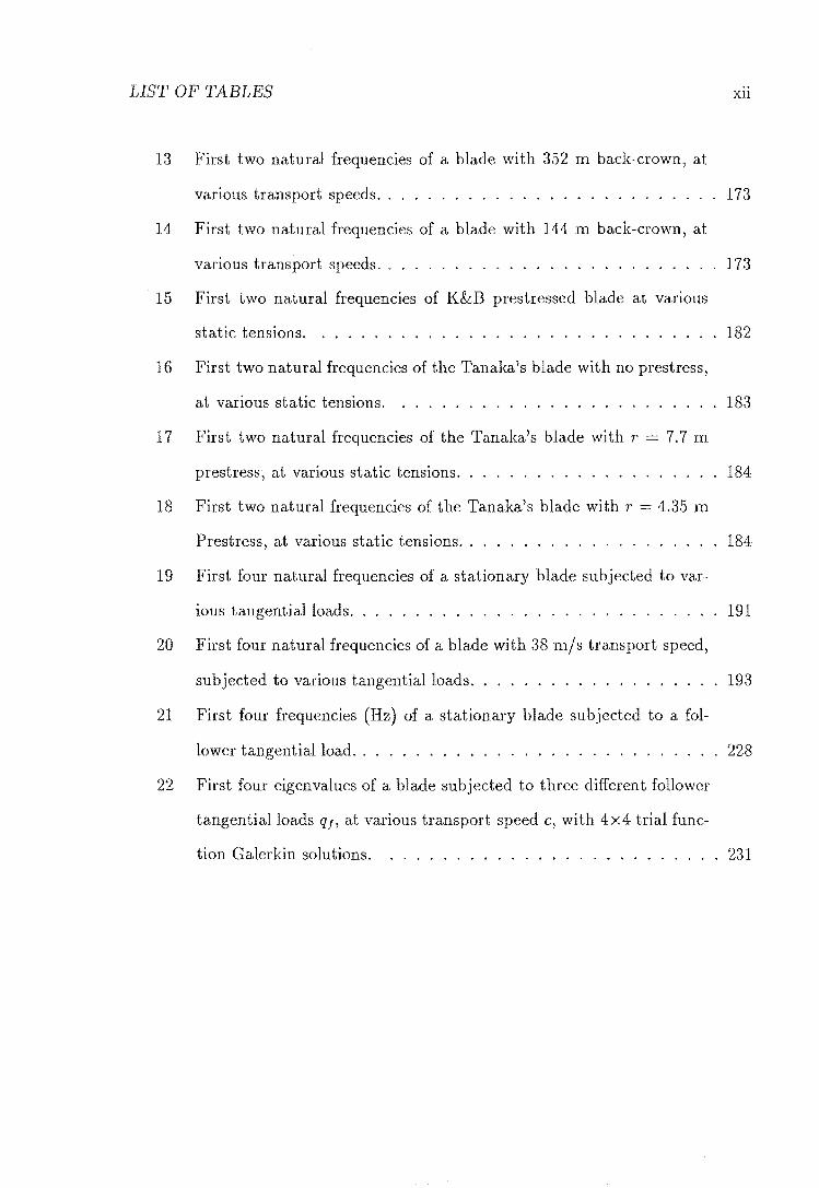
13 First two natural frequencies of a blade with 352 m back-crown, at
various transport speeds .......................... 173
14 First two natural frequencies of a blade with 144 m back-crown, at
various transport speeds. . . . . . . . . . . . . . . . . . . . . . . . . . 173
15 First two natural frequencies of K&B prestressed blade at various
static tensions. .... . . . . . . . . . . . . . . . . . . . 182
16 First two natural frequencies of the Tanaka's blade with no prestress,
at various static tensions. 183
17 First two natural frequencies of the Tanaka's blade with r = 7.7 m
prestress, at various static tensions. . . . . . . . . . . . . . . . . . . . 184
18 First two natural frequencies of the Tanaka's blade with r = 4.35 m
Prestress, at various static tensions. . . . . . . . . . . . . . . . . . . . 184
19 First four natural frequencies of a stationary blade subjected to var-
ious tangential loads ............................ 191
20 First four natural frequencies of a blade with 38 m/s transport speed,
subjected to various tangential loads ................... 193
21 First four frequencies (Hz) of a stationary blade subjected to a fol-
lower tangential load. . . . . . . . . . . . . . . . . . . . . . . . . . . . 228
22 First four eigenvalues of a blade subjected to three different follower
tangential loads q" at various transport speed c, with 4x4 trial func-
tion Galerkin solutions. . ........................ 231

o
1 Fi
1 General assembly of a 60 in. band head rig. Right side view. 13
2 General assembly of a 60 in. band head rig. Front view .. 14
3 Back view of the Waimak bandsaw. 15
4 Left view of the Waimak bandsaw. 17
5 Right view of the Waimak bandsaw .. 18
6 Column slide. .. 20
7 Lower saw guide. 21
8 Upper saw guide. 21
9 Non-cutting span damper. 22
10 Counterweight straining mechanism. 23
11 End view of rocker shaft. 24
12 Spring and swage set. 24
13 Dimensions of teeth. 26
14 Aliasing effect in discrete sampling of signaL 31
15 Actual signal and FFT assumed signal. 32
16 The effect of windowing. . . . ,. . ~ ,. ,. 33
17 Typical impact force pulse and spectrum .. 33
18 Positive sign convention. . ,. ,. ,. . ,. ..... 40
19 Generalised coordinates for longitudinal vibration. 43
Xlll

LIST OF FIGURES
20 Generalised coordinates for torsional vibration.. . . 43
21 Generalised displacements for a 3D beam element. . 45
22 Angular displacements in a symmetrical rotor. 46
23 Third mode of a portal frame. . . . . . 50
24 Global coordinates in three dimensions. 51
25 Local and global degrees of freedom of node n. 52
26 Third node of a beam element. 54
27 Secant's and Muller's methods. 56
28 Hierachical structure of the program. 60
29 Mode shapes of the base. 64
30 Section below the base. . 65
31 Frequency spectrum of a response of the section below the base. 65
32 Model mesh. . 67
33 First mode. 67
34 Second mode. 68
35 Third mode. . 68
36 Fourth mode. 69
37 Fifth mode. 69
38 Main components of the section above the base. 70
39 Frequency spectrum of the side-to-side transverse vibration. 71
40 Frequency response function of the side-to-side transverse vibration. 72
41 Frequency spectrum of the to-and-fro transverse vibration. . . . .. 72
42 Frequency response function of the to-and-fro transverse vibration. . 73
43 Main column. . . . 74
44 First model mesh. . 75
45 First mode shape of the first model. . 76

LIST OF FIGURES
46
47
48
49
50
51
52
53
54
55
56
57
58
59
60
61
62
63
64
65
66
Second mode shape of the first model.
Third mode shape of the first modeL
Second model mesh.
First mode shape of the second modeL
Second mode shape of the second model.
Third mode shape of the second model. .
Fourth mode shape of the second model.
Fifth mode shape of the second modeL .
Frequency response function of the straining device, 0-10 Hz.
Frequency spectrum of the straining device, 0-100 Hz. . . . .
Frequency response function of the straining device, 0-100 Hz.
Model to represent the rigid body mode of the straining device.
The variation of the natural frequencies, Wi, of the bandsaw structure
below the base, with pulley rotating velocity, n. . . . . . . . . . . . .
The variation of the natural frequencies, Wi, of the bandsaw structure
above the base, with pulley rotating velocity, n. . . . . . . . . .
Spectrum of the vibration during idling in the vertical direction.
Spectrum of the vibration during idling in the to-and-fro direction.
Spectrum of the vibration during idling in the side-to-side direction.
Bearing dimensions ............... .
Frequency spectrum of a truncated sine wave.
Effective span length in a pressure guide system ..
First four modes of a three span beam with no tension.
67 First four natural modes of a three span beam with 0.786 m, 1.0 m,
xv
76
77
77
78
78
79
79
80
81
82
83
84
86
88
89
90
90
91
93
. 104
. 108
0.5 m span lengths under no tension ................... 110
LIST OF FIGURES XVl
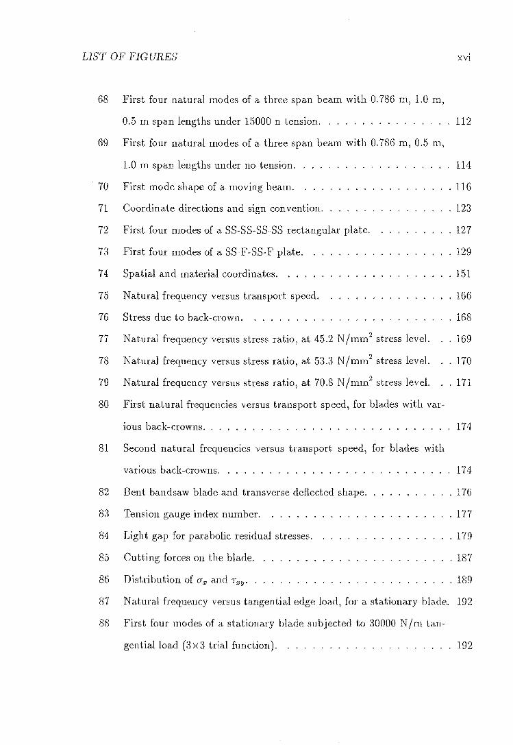
68 First four natural modes of a three span beam with 0.786 m, 1.0 m,
0.5 m span lengths under 15000 n tension. . .............. 112
69 First four natural modes of a three span beam with 0.786 m, 0.5 m,
70
71
72
73
74
75
76
77
78
79
1.0 m span lengths under no tension.
First mode shape of a moving beam.
Coordinate directions and sign convention.
First four modes of a SS-SS-SS-SS rectangular plate.
First four modes of a SS-F -SS- F plate.
Spatial and material coordinates. . . .
Natural frequency versus transport speed.
Stress due to back-crown.
Natural frequency versus stress ratio, at 45.2 N/mm2 stress level.
Natural frequency versus stress ratio, at 53.3 N/mm2 stress level.
Natural frequency versus stress ratio, at 70.8 N / mm2 stress level.
80 First natural frequencies versus transport speed, for blades with var-
ious back-crowns. . . . . . . . . . . . . . . .
81 Second natural frequencies versus transport speed, for blades with
various back-crowns. . . . . . . . . . . . . .
82
83
84
85
Bent bandsaw blade and transverse deflected shape.
Tension gauge index number.
Light gap for parabolic residual stresses.
Cutting forces on the blade.
114
116
· 123
· 127
· 129
· 151
166
168
· 169
· 170
171
174
174
· 176
177
179
· 187
86 Distribution of o"x and Txy. • • 189
87 Natural frequency versus tangential edge load, for a stationary blade. 192
88 First four modes of a stationary blade subjected to 30000 N/m tan-
gentialload (3x3 trial function). . ................... 192

LIST OF FIGURES XVll
89 Natural frequency versus tangential load, for a blade with 38 l1i/S
transport speed. 194
90 Instability regions for the first transverse mode of a stationary blade
subjected tofiuctuating tensions, with a one-term Fourier expansion. 206
91 Instability regions for the first transverse mode of a stationary blade
subjected to fiuctuating tensions, with a two-term Fourier expansion. 207
92 Instability regions for a 2x2 trial function Galerkin solution of a
stationary blade subjected to fluctuating tensions, with a two-term
Fourier expansion. ... . . . . . . . . . . . . . . . . . . . . . . . . . 208
93 Instability regions for a 2x 1 trial function Galerkin solution of a mov-
ing blade, with c = 40 mis, subjected to fluctuating tensions,
with a two-term Fourier expansion. . . . . . . . . . . . . . . . 210
94 Inclination of the left boundary of the 2ft simple parametric reso-
nance region versus transport speeds, c.
95 Instability regions for a 2x2 trial function Galerkin solution of a sta
tionary blade sub.jected to periodic tangential cutting forces, with a
211
two-term Fourier expansion. . . . . . . . . . . . . . . . . . . . . 214
96 Instability regions for a 2x2 trial function Galerkin solution of a
moving blade subjected to periodic tangential cutting forces, with a
two-term Fourier expansion ........................ 216
97 Inclination of the left boundary of the 11 + h combination parametric
resonance region versus transport speeds, c. ., . . . . . . .
98 Load versus frequency for a beam under unidirectional force.
99 Root-locus diagram for a beam under unidirectional force.
100 Follower force on a cantilevered beam. . ....... .
101 Load versus frequency for a beam under follower force.
216
.'. 218
. 219
. 219
.220

LIST OF FIGURES
102 Root-locus diagram for a beam under follower force.
103 Conservative force field. .............. .
104 Three ways in which a beam attains its final state ..
105 Follower tangential force on a saw blade.
106 Components of the follower force .....
107 Eigencurves for a stationary blade subjected to a follower tangential
XVlll
. 221
. 221
.222
.223
.224
edge load. . . . . . . . . . . . . . . . . . . . . . . . . . . . . . . . . . 229
108 First three modes of a blade subjected to 20000 N/m follower tan-
gentialload, with a 3x3 trial function Galerkin solution. . ...... 230
109 The first mode and the unstable mode of a blade subjected to 36200 N / m
follower tangential load, with a 3x3 trial function Galerkin solution. 231
110 Root-locus diagram for the the first three eigenvalues of a blade, at
c =40 m/s. . ............................... 233

c
IN DU TI N
The main objectives of the saw milling industry are:
411 To produce a straight, smooth cut at maximum speed and with a minimum
loss of raw material, for a wide range of timber types and depths of cut.
It To spend as little as possible on the maintenance and down time costs of the
machinery used.
The bandsaw has become a very important machine in the sawing process be
cause:
• It has the thinnest blade among all the wood cutting machines, therefore
minimizes the wastage of material.
• It operates at a very high cutting speed, allowing higher production rates than
other types of saws.
• It is capable of handling a large range of log sizes.
• It usually operates at lower noise levels than other types of saws, such as the
circular saw.
1

CHAPTER 1 2
Transverse vibration of the bandsaw blade is a by-product from the interactions
of the blade with the machine structure and the timber being cut. It increases
the amount of saw dust produced, decreases the accuracy of the cut, decreases the
production rate and decreases the life of the blade. In the last 25 years, engineers
and foresters have been trying to reduce the vibration of the blade from experimental
and theoretical studies. A vast knowledge on the behaviour of the moving bandsaw
blade has been gained, however, many mysteries still remain in this area of research
which have to be solved in order for the technology to advance in the future.
There have been complaints recently in New Zealand that the bandsaw structures
inhere considerable vibrations, which cause annoyance to workers and increase the
risk of machine failures. These complaints have initiated this project which proposed
to look into the structural vibration of the bandsa-w. A literature search showed that
there has never been any consideration on the vibration of bandsaw structure, all
previous reseach has been directed toward the cutting span of the saw blade.
The behaviour of the saw blade during sawing is another area of great interest,
which needs a lot more attention in the future. This project, therefore, attempts to
investigate the cause of instability of the blade during sawing. This area of research
will become necessary in the development of automatic control of the timber cutting
process.
1.1 Historical Background
The work to be presented in this thesis requires the materials in three different fields:
• Structural vibrations
• Dynamics of bandsaw blades
• Dynamics of plates

CHAPTER 1 3
1.1.1 Structural Vibrations
Theoretical analysis of structural vibrations has been well documented in many vi
bration text books and taught in undergraduate vibration courses, however, there
seems to be a lack of unification in the methods of solution. The advances com
puter technology also have affected many of these methods, offering better methods
of analysis, allowing more complex problems to be solved, and making some methods
obsolete.
Bishop and Johnson (1956) [10] and McCallion (1973) [48] presented comprehen
sive backgrounds on the theory of beam vibrations. The method of analysis used in
this thesis, the dynamic stiffness method, was developed by Kron (1939,1963) [40,41]
and was reinterpreted into a more easily understood form by McCallion (1973) [48].
Other publications involving the use of the dynamic stiffness method include Rieger
and McCallion (1965) [65,66], Henshell et.al. (1965)[29], Palmers and McCallion
(1973) [61], Williams and Wittrick (1970) [92], Howson (1979) [33].
The mathematical algorithms to perform various numerical operations, such as
calculating determinants of matrices, finding roots of equations etc. , are well pre
sented in many numerical methods text book, notable is the Numerical Recipes
(1986) [63]. Other cited references, relating to numerical methods, are [51,74].
The theory on the gyroscopic effects of rotors refers to the publications by Ware
(1978) [90], McCallion (1973) [48] and Downham (1957) [21,22].
The experimental analysis of structural vibrations has been the subject of many
researches in recent years because of the advances in electronics and computer tech
nologies. A most up to date text book on this topic is the book written by Ewins
(1984) [23] who is one of the leading experts in the field of modal analysis. Other
references relating to this area of research, vvhich had been cited for this thesis, were
[28,69,30,31,18,70] .

CHAPTER 1 4
1.1.2 Dynamics of Handsaw lades
Most of the research on bandsaws was carried out in the last two decades. Ulsoya,nd
Mote (1978) [85] published a comprehensive literature review which listed 115 pub
lications in relation to the bandsaw problems. D'Angelo et.aL (1985) [16] provided
a more recent list of research being carried out on circular and band saw vibration
and stability.
This literature review will categorise some of the more relevant research, instead
of attempting to list all the research relating to band saw problems.
The literature on bandsaws can be classified into 9 topics:
III General information on bandsaws.
• Experimental studies in the free vibration of saw blades.
41 Experimental studies of the blade during sawing.
• Stresses in bandsaw blades
III Theoretical studies on the free vibration of moving materials.
III Theoretical studies on the stability and vibration of moving materials due to
external and parametric excitations.
III Studies on the coupling between cutting span and non-cutting span of the saw
blade .
., Nonlinearities in moving materiaL
Saw guides

CHAPTER 1 5
General information
The most informative text book on the subject of bandsaws is the book by Simmonds
(1980) [71], which includes up to date technology in the art of saw doctor·ing. Other
books, discussing the use of bandsaws, include [93,91]. The manufacturers also have
a large amount of information on the design and operation of bandsaws.
This information is the prerequisite in any study on bandsaw. It forms a direct
link between researchers and the industry.
Experimental Studies - Free vibration
There are many publications in this topic, but the Inost noteworthy works were by
Kirbach and Bonae (1978) [37,38], and by Tanaka et.al. (1981) [80]. These publica
tions provided the natural frequencies of bandsaw blades wi th various dimensions,
velocities, and stresses.
Experin'lental Studies - During Sawing
The subject of bandsaw vibrations during sawing is slightly touched on in recent
years, perhaps because it is rather costly and difficult to investigate the behaviour
of the saw blade during sawing. There have not been any conclusive results in
this area of research. Das (1982) [17] demonstrated the existence of instability
during sawing, unfortunately, not enough information was given in the paper to draw
any conclusion. Tanaka et.al. (1983) [81] also investigated the saw blade vibration
during sawing, the results presented however, seemed to lack practical intuition, for
example, one of the conclusions was that the timber being cut clamps the blade
hence acts as a boundary support for the top part of the blade.

CHAPTER 1 6
Stresses in bandsaw blades
This is a very important topic in the design of a saw blade. In-plane stresses dom
inate the stiffness of the blade and their effects on the vibration and stability of
the blade are considerable. Pahlitzsch and Puttkammer (1972) [60] discussed the
stresses occurred on the blade. A more cornprehensive work on the same topic was
presented by Allen (1985) [3], which suggested that by applying higher strain on the
blade, the stability under cutting conditions was improved. The problem is that too
much strain will cause failure of the blade, however, investigations of these stresses
have only used basic theories of strength of materials or have been based on ex
perimental measurements. A more comprehensive study is yet to be carried out so
that a maximum strain can be put on the blade with confidence. Foschi (1975) [25]
who investigated the technique of measuring residual stresses in bandsaw blades,
concluded that the present method, the light gap technique, was not reliable, but
did not suggest any alternatives.
Theoretical Studies Free Vibration of Moving Materials
This topic provides the foundation for all the theoretical works on vibration and
stability of the moving bandsaw blade.
The first investigation was dated back to 1897 when Skutch [73] studied the
transverse vibration of an axially moving string. It was not until 1965 when the first
study of the bandsaw blade was carried out by Mote [52,53]' which considered the
transverse vibration of a moving beam, using the exact method. Later, Anderson
(1974) [6] looked at the same problem using a finite element method which allowed
moving beams with more complex boundary conditions to be solved. Alspaugh
(1967) [5] considered the torsional vibration, and in 1968, Soler [75] looked at the
coupling between transverse and torsional vibration. Ulsoy and Mote (1980,1982)

CHAPTER 1 7
[86,87] produced excellent works on the vibration of moving plates to represent wide
saw blades.
Theoretical Studies - ParaInetric and Direct Excitations
An understanding of the behaviour of a moving saw blade under excitations is impor
tant in the design of the blade. Naguleswaran and \,yHliams (1968) [58] investigated
the stability of moving beam under fluctuating tension. This tension fluctuation is
caused by pulley eccentricities, irregularities on the surface of pulleys and the sur
face of blade. Ariaratnam and Asokanthan (1988) extended the study to torsional
vibration using the method of averaging. Soler (1968) [75] looked at a point load,
perpendicular to the longitudinal direction of the blade, to approximate the cutting
condition. Mote (1968) studied the divergence buckling of an edge loaded beam
[55], the parametric instability of beams under fluctuating tension (similar to [58]),
and the parametric instability of beams under periodic edge force. In 1986, Wu
and Mote went back to this periodic edge loading on beams but also considered the
coupling between transverse and torsional vibrations.
There has been no study in the area of parametric stability using a moving plate
model to represent the wide saw blade. Ulsoy and Mote (1980) [86] briefly mentioned
the effects of edge loadings on a moving plate but concluded that the magnitudes of
these forces were small compared with other effects, such as tension on the blade.
Coupling between Cutting and Non-cutting Spans
This is a new area of research with the first experirIlental observations of the coupling
in 1984 by \,yu and Mote [94]. A full theoretical investigation of the coupling, using
transverse vibration of moving beam, was carried out by Wang and Mote (1986)
[88]. In 1987, Wang and Mote [89] looked at the vibration of the same coupling

CHAPTER 1 8
system under impulsive excitation.
Nonlinear Vibration of Axially Moving Materials
Mote (1966) discussed the nonlinear vibration of an axially moving string due to
a large amplitude of vibration at high axial velocity and low tension. Thurman and
Mote (1969, 1971) extended this to a moving beam, and showed that nonlinearities
result in the coupling between transverse and longitudinal vibrations. Kim and
Tabarrok (1972) [36] again investigated the nonlinear vibration of travelling strings,
using a differen t approach based on the theory of fluid mechanics.
The above publications stated that this area of research was very significant.
However, it has been ignored by recent research, perhaps because of its complexity,
or perhaps because of its impracticability in the bandsaw blade case.
Saw Guides
This area of research was not considered in this thesis, but is mentioned here for the
sake of completeness.
The effects of saw guides on the vibration of bandsaw blade are well observed
in practice, however there is a lack of theoretical background on the guides. Only
recently, Tan and Mote (1988) [79] treated the guides as hydrostatic bearings and
investigated their effects on the vibration of saw blades.
1. 1.3 Dynamics of lates
The theory on plate stability and vibration are required in this thesis to model the
wide bandsaw blade. A thorough understanding of the plate theory is necessary to
develop a sound method of analysis for the moving plate.
The basis of plate theory is in many vibration text books [48, page 125], and

CHAPTER 1 9
there are text books devoted entirely to plate theory [76,35]. Leissa (1969,1973)
[45,46] provided an extensive study of the vibration of a rectangular plate under all
combinations of boundary conditions; using the exact method where possible and
the Ritz method for the remaining cases. Young (1950) [97] had already considered
the rectangular plate problems using the Ritz method.
By using approximate methods, such as the Ritz method or the GalCl'kin method,
shape functions which describe the deflections of the plate are required. The con
ventional shape functions are the separable beam functions for each direction [76,
page 228]. Bassily and Dickinson (1975) [8] suggested the use of degenerated beam
functions for plates involving free edges. More recently (1985,1986), orthogonal
polynomials had been suggested as a better alternative for choosing shape functions
for plates [9,19].
Zienkiewicz and Morgan (1983) [99] provided a powerful reference on the methods
of approximation which has been used to solve the plate problems presented in this
thesis.
Two types of dynamic stabilities had been considered in this study; parametric
and nonconservative.
Takahashi and Konishi (1988) [78,72] considered the stability of a rectangular
plate subjected to parametric excitation. References to the method of analysis, the
harmonic balance method, are in [12,59,50,77,24,62].
The stability of rectangular plates subjected to nonconservative loadings has been
studied by Leipholz (1982,1983) [43,44] using Galerkin method. The foundation for
this area of research is the text book written in Russian by Bolotin (1961) and
translated to English in 1963 [11]. Other related publications include [1,32].

CHAPTER 1 10
1.2 s e of the roject
The first part of the project was to study, experimentally and theoretically, the
vibrational characteristics of the bandsaw structure. This work was aimed primarily
at developing a technical knowledge in the field of vibrations, and secondly at viewing
the practical aspects of the problem. The results found in this work could be used
to reduce the vibration of the bandsaw structure or to see if they could affect the
performance of the saw blade. An important effect to be investigated was the
gyroscopic effect of the rotating pulleys.
A more powerful method of solution for the moving beam case has been developed
111 Chapter 6. Although there have been acceptable methods for this problem,
the new method of analysis is believed to be simpler and can provide much more
informative solutions than previous methods. Interactions between the blade and
the structure can be investigated by this method.
Another method of analysing the moving plate problem was developed in Chap
ter 7, which can be extended from the usual vibration case to the more complicated
stability problems. This method has been used to calculate the natural frequencies
of bandsaw blades with various in-plane stresses.
Parametric excitations on a moving plate have been studied in this project, which
are closely related to the moving beam case, but would offer much more accuracy
and flexibility in the study of wide bandsaw blades.
A study of stability of a moving plate under nonconservative cutting forces is
presented, for the first time, in this thesis. The results are very encouraging and an
experimental study would be necessary in the future to back up these results.

t 2
H D SI FA A
A S
2.1 eneral Assembly
There are many types and sizes of bandsaws used in the sawmilling industry today.
The most common type is the vertical log bandsaw (Figure 1,2), and therefore, the
structural vibration study will consider primarily this type of bandsaw. The blade
behaviour would be the same whether the bandsaw was of the vertical or horizontal
type.
The classification of a bandsaw is by the diameter of the saw pulleys - typical
sizes are 48 in., 54 in., 60 in .. The bandsaw, selected for the experimental study,
was a 60 in. bandsaw, manufactured by the Southern Cross Engineering Company
and installed at the Waima,kariri Sawmill (referred to as the Waimak bandsaw).
The main structures of the vertical bandsaw are best subdivided into three sec
tions:
• Section below the base.
11

CHAPTER 2 12
IIJ Section above the base.
til The straining device.
The saw blade is an independent component of the bandsaw hence it is treated
separately.
From now on, the front of the bandsaw refers to the cutting side of the saw as
shown in Figure 1.
.2 Section Below the ase
The base itself is usually bolted down to the foundation for maximum rigidity. A
pit is, therefore, required for the portion of the bandsaw below the base. However,
there are installations which raise the base above ground level. These bandsaws may
have large vibrations at low natural frequencies, due to weak supports.
Figure 3 shows the back view of the bandsaw looking into the pit.
The section of the bandsaw below the base consists of
Bottom Pulley It is usually made of cast iron. The boltom pulley) being the
driving pulley, is stronger (bigger spokes) and therefore heavier than the top
pulley. The pulley of the Waimak bandsaw has a diameter of 60 in. (1.5 m),
weighs about 550 kg. It has eight spokes, each about 0.1 m in diameter.
Shaft The bottom shaft is 1.6 m long and 0.1 m in diameter. The pulley is mounted
close to one end of the shaft as in Figure 2. This asymmetrical mounting may
produce some interesting phenomena.
Bearings Two '22222 K .1I. L. H322 4in.' spherical-roller bearings are used to sup
port the bottom shaft. The housing for each bearing is bolted to a bracket by

CHAPTER 2
,.
Top Pulley
Beai'ing
Main C olumn ---~~-m~~~1I,
Column S Ii d e ---,---~-+",:,,-~:::,,<;;'.J.1
Strain Lever----......,
Bottom Pulley-, ---""';';"-':""'''''''\:1'
·1
',',
' ....
::. Front ......... V· .: . lew
.. ~ "
"-::--1 ", ," .
< "
'.' , , . :- ~
"'0 "'"
Figure 1: General assembly of a 60 m. band head rig. Right side view.
13

CHAPTER 2 14
'.
r'-'
..... \ :,',- ".'h-: . I'· ,t·'
•• : I' .... ~:: .. " .... r ,
-' I ,
(',;;
'I
--=-l
Figure 2: General assembly of a 60 m. band head rig. Front view.

CHAPTER 2 15
FjgLlre 3: Bac k view of the Waimak bandsaw.

CHAPTER 2 16
four 20 mm bolts. The bracket is fabricated from 20mm plate and is welded
to the base.
lV(otor and Transmission The bandsaw is driven by an electric motor, and the
transmission of power to the bottom pulley is by V-belts.
2. Section Above the ase
Figure 4 and Figure 5 show the left and the right views of the Waimak bandsaw
respectively.
These figures show that the structure of the top section of the band saw is quite
complicated. It is, therefore, expected that the theoretical calculations based on
beam theory will not provide accurate values for the natural frequencies of the
bandsaw. The beam model would still be important in understanding the general
vibrational characteristics, and in explaining the experimental results.
The main components of the bandsaw are:
Main ColuHm It is extended vertically from the base, and fabricated from mild
steel plate. It provides the skeleton for the bandsaw.
Column Slides There are two column slides which are guided vertically by the
main column. They can be driven up and down by two jack assemblies. Fig
ure 6 shows a side view of the column slide. At the front of the column slide
is another slider where the top saw guide is attached. The bearing housing is
pinned to the top of the column slide.
Top Pulley The top pulley is mounted on the column slides so that it can be moved
to tension the saw blade.

CHAPTER 2 17
fi gur e 4 Left vie w of th e Waimak bandsaw.

CHAPTER 2 18
FIgure 5: RIght view of the Waimak bandsaw.

CHAPTER 2 19
Bearings The bearings used to support the top pulley are identical to those for the
bottom pulley. The column slides are locked in position after tensioning the
saw blade. To prevent the tension on the blade changing excessively during
starting-up or while cutting, there is a dead load straining mechanism. The
bearing housings are pinned to the column slides so that they can be rotated
relative to the fixed column slides.
Saw Guides Saw guides are used to reduce the vibration of the saw blade and
hence increase the blade's stability. There are several types of saw guides but
the most common type used in wide-band bandsaws is the pressure guide. The
lower guide is fixed in place so that it supports the blade immediately below
the work piece, see Figure 7 . Dense woods or synthetic materials are used for
the packings. A 0.005 in. clearance between the packings and the saw blade
is recommended. The upper guide, Figure 81 can be moved up and down to
adjust for a range of depths of cuts. The pressure guide is pressed against one
side of the blade. It was found that vibrations on the non-cutting span can
be transmitted to the cutting span, and a damper is usually fitted to reduce
2
the vibrations of the non-cutting span, Figure 9.
a cleaning device for the saw blade.
training Device
damper is also used as
The most common straining de~ice is the counterweight and lever mechanism. Fig
ure 10 shows the components of the straining mechanism. The counterweight mech
anism is analogous to the spring-mass system, where the blade behaves as an elastic
spring and the counterweight is the mass.
In modern bandsaws, air strain devices are used because they have faster response

CHAPTER 2 20
Figure 6: Column slide.

CHAPTER 2 21
Figure 7: Lower saw guide.
figure 8: Upper saw guide.

CHAPTER 2 22
Figure 9: Non-cutting span damper.
times than the dead weight mechanism. However, there are still many bandsaws in
operation today using the simple counterweight and lever device.
2.5 Saw Blade
From the definition given in [71], a \-vide bandsaw blade is any blade which has at
least 76 mm in width. For the Waimak bandsaw, a 240 mm wide blade is used. This
size of saw blade is also used in the experiments of Kirbach and Bonac [37,38]. The
total length of the blade is about 9.75 m (32 ft), and the thickness is approximately
1.6 mm.
There are two types of tooth sett ing for saw blades; spring set and swage set.
Spring set is when the teeth are bent alternatively on either sides of the blade, and
swage set is when the tip of the tooth is made wider than the thickness of the blade
to provide clearance [or the cut (Figure 12) .

CHAPTER 2
II
Bearing Hous'lflg
~---+------f---I-S train Bar I
I
I: : I
r---t-L---------j--F U lcr u m
LI _______ '
II II I
1,1
Shaf t
'-----------------t-Lever Arm
23
~--------------------------(ounterweight
Figure 10: Counterweight straining mechanism,

CHAPTER 2
Figure 11 : En d vie w of rocker shaft .
""[:: ,.111111'''''''[:: ""IIIIIII"IIc:::IT# ~ , 1 1 I t I"" I 1 1 , • " 1 • , C' I 1 " 1 " 1 II I 1 " t:50i ~
C:::; Width of Kerf (1 Tooth) Swage Set
D:::; Width of Kerf (2Teeth) Spring Set
Figure 12 : Spring and swage set.
24

CHAPTER 2 25
Swage setting is now accepted as being the better method of the two and spring
setting method is, therefore, becoming obsolete.
Dimensions and profile of the teeth on the blade used on the Waimak bandsaw
are given in Figure 13.
book, by Simmonds [71], provides full details of the manufacture and prepa
ration of wide bandsaw blades. The two techniques, widely used in the preparation
of saw blades to improve its performance, are the prestressing and the back crowning.
Both alter the stress states of the blade and hence modify its dynamic characteris
tics. This thesis will consider theoretically the effects of both prestressing and back
crowning, by using plate theory, because they cannot be predicted by beam analysis.

CHAPTER 2 26
0·22
0·24
Figure 13: Dimensions of teeth.

E IMEN M THO
ST URAL RATI
3.1 duction
The two major objectives of vibration measurement, as stated by Ewins [23], are
• To determine the nature and extent of vibration response levels.
• To verify theoretical models and predictions.
These two objectives indicate the two types of test used in the experimental
analysis. The first objective corresponds to the measurement of vibrations of the
machine or structure under study during operation, and the second objective requires
the measurement of vibrations with known excitations.
Both types of test were performed on the Waimak bandsaw. Experiments carried
out on a prototype bandsaw in a laboratory would be ideal, unfortunately, such an
arrangement was not available. Tests on real operational bandsaws are not as flexible
but realistic results can be obtained.
27

CHAPTER 3 28
3.2 General rocedure in Experimental Analy-
Vibration measurement of a machine during operation requires no special technique
and can be performed with the equipment used in the vibration measurement with
known excitations.
The vibrational characteristics of a structure, with known excitations, can be
obtained in three stages. First the structure has to be excited, then the vibrations
of the structure can be measured and recorded, and finally, the recorded data can
be analysed.
3.2.1 Excitation of the Structure
The two types of excitations are continuous excitation such as sinusoidal, random
etc. , and transient excitation such as pulse, chirp, impact.
Devices available for exciting the structure can be devided into two categories:
contacting and non-contacting.
Contacting exciters remain attached to the structure throughout the test. Some
commonly used contacting exciters are mechanical exciters (out-of-balance rotating
masses), electromagnetic exciters (moving coil in magnetic field), and electrohy
draulic exciters.
Non-contacting exciters include non-contacting electromagnets, and impactors
which are only in contact for a short period.
The object of using the exciter is to excite the structure over a range of frequen
cies so that the frequency response characteristics of the structure can be determined.
The best method is the sinusoidal excitation where the exciting frequency can be

CHAPTER 3 29
controlled over the range of interest. However, the instruments for sinusoidal ex
citation can be expensive and impractical, especially for a structure such as
the bandsaw. Impact excitation is applicable in the low range of frequencies and
no or very little prep~ration on the structure is needed before using the impactor.
Small explosive charges had been successfully used as an impact exciter on structures
where access to the structure was not possible during tests, such as aeroplane wings
during flight. Other possible impactors are hammers, hanging masses or sudden
release of statically deformed structures.
3.2.2 Measurement of the Vibrations and the Excitations
The vibration of the structure can be measured as displacement, velocity or accelera
tion, of which acceleration is the most popular and the most practical measurement.
Acceleration is measured by accelerometers whereas the exciting force can be mea
sured by force transducers. Both of these transducers are piezoelectric transducers
which produce voltages for the vibratory motions or the exciting forces.
There are two types of vibration measurement techniques; those which just
one parameter is measured (usually the response), and those in which both input
and output response are measured. If only the natural frequencies of the structure
are of interest, then measurement of one parameter is sufficient, but if the levels of
the vibrations are also important then measurement of two parameters would give
much greater accuracy.
The voltage produced is very small and conditioning amplifiers are required to
boost the signal up to a measurable amount. Voltage amplifiers and charge amplifiers
are the two types of conditioning amplifiers available.
Measured data can be stored using a multi channels FM tape recorder. This
data is then post-processed by using an analyser. Modern FFT analysers enable

CHAPTER 3 30
the signals from the transducers to be processed instantanously and store on floppy
disks) however) tape recordings are still useful in keeping a full real-time record of
the response.
3 .3 Analysis
The recorded vibration data needs to be processed into a more practical form. For
the one parameter measurement technique) Fourier analysis transforms the data
from the time domain to the frequency domain so that any nat ural frequencies of
the structure at the point of measurement can be seen from the spectrum. The other
technique, where both the vibratory motions and the excitations are measured, is
analysed by obtaining the frequency response function of the structure. The methods
available for plotting the frequency response function had been discussed in [23].
Modern analysers have built-in functions to produce plots of frequency response
functions from the input and output data.
There are many problems associated with digital spectral analysis. Although
modern FFT analysers are designed to take care of most of these problems, knowl
edge of them is necessary in interpreting the FFT results.
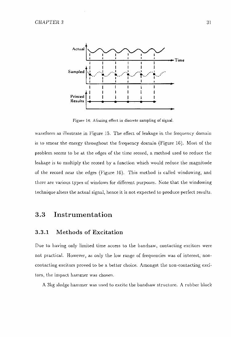
Alias is a problem caused by discrete sampling of the signal (Figure 14), where
the FFT result does not represent the actual signal. To overcome this problem
the sampling frequency must be more than two times the maximum frequency of
interest; anti-alias filters are also required to screen out frequencies higher than the
sampling frequency.
Leakage is a problem caused by the recording of the signal over a finite interval.
Transient signals do not have leakaging problems, but periodic signals do. This
problem is caused by an assumption in the FFT algorithm that the finite-time-record
is repeated throughout time. This assumption can sometimes produce a distorted
CHAPTER 3 31
AC'Uall .... ..:.: __ ..;..._-.;. __ ..;... ____ ~--....... Time , I
Sampled .... 1 .. ' ".1 , •.. I •• ) , •• .1 ," I •••• •. .. ' " ,,' •. .. ' t··... ., , I" " ," I" I" I I I
r I
Primed I Resuhs ~.t---1 ..... - ........ - .... ~--1 ..... - .... ~
Figure 14: Aliasing effect in discrete sampling of signal.
waveform as illustrate in Figure 15. The effect of leakage in the frequency domain
is to smear the energy throughout the frequency domain (Figure 16). Most of the
problem seems to be at the edges of the time record, a method used to reduce the
leakage is to multiply the record by a function which would reduce the magnitude
of the record near the edges (Figure 16). This method is called windowing, and
there are various types of windows for different purposes, Note that the windowing
technique alters the actual signal, hence it is not expected to produce perfect results.
3.3 Instrumentation
3.3.1 Methods of Excitation
Due to having only limited time access to the bandsaw, contacting excitors were
not practical. However, as only the low range of frequencies was of interest,' non-
contacting excitors proved to be a better choice. Amongst the non-contacting exci-
tors, the impact hammer was chosen.
A 3kg sledge hammer was used to excite the bandsaw structure. A rubber block

CHAPTER 3 32
21) Actual input
b) Time record
I c) Assumed inpul
Figure 15: Actual signal and FFT assumed signal.
was glued to the hammer head to prevent damage to the bandsaw when impact
ing the structure. Because a force transducer was not available, an accelerometer
was used instead, and the hammer was calibrated so that the readings from the
accelerometer gave the amount of force applied.
Figure shows a typical impulsive force pulse, it was approximately a half-sine
wave. Fourier transformation of this pulse gave the frequency spectrum which was
essentially fiat up to a certain frequency, fe. This fe is the upper frequency range of
the hammer. The sledge hammer used in this experiment was effective up to 350 Hz.
3.3.2 Vibration Measurement Techniques
Ten accelerometers were available for this experiment. Two Bruel & Kjael con
ditioning amplifiers and eight home-made charge amplifiers were used with these

CHAPTER 3
: d) Actual input
I T' 1 ~ Ime Io--l I Record I
I
1 I 1 I I b) ::1\1 1 I I I
I 1 c) 1 I I I
1 1 1 1 1
Assumed input
Window (unction
~) Windowed input
Figure 16: The effect of windowing.
F("UJ)
ttt)
t
(0 l (b) Hz
Figure 17: Typical impact force pulse and spectrum.
33
Hz
Hz
Hz

CHAPTER 3 34
accelerometers.
There are several methods of attachment of accelerometer to the structure. Some
of the common methods are threaded stud [which requires modification to the struc
ture and was hence undesirable]' cemented stud, thin layer of wax, and magnet. The
choice of attachment method determines the range of frequency the accelerometer
can measured. Magnetic attachment was used. It has low useful frequency range
(0 Hz 1000 Hz), but was acceptable for this experiment.
For experiments requiring multiple accelerometer readings instantaneously, the
signals were recorded on an eight channels Hewlett-Packard tape recorder, and for
those requiring only one or two inputs, the signals were read and recorded directly
by the FFT analyser.
3.3.3 FFT Analyser
An Iwatsu SM-2701 FFT analyser was used for analysing the data. It had many
built-in functions for vibration and sound analyses. For the bandsaw experiments,
only three functions were used; the time domain measurement, the frequency do
main measurement (Fourier transform of the time domain data), and the frequency
response function measurement.
Even though, no major problems were encountered in using the FFT analyser,
an experience user could have saved a lot of time in setting up the equipment, and
producing and storing the required data.

c e
T R CA M o
TRUCTU L o s
4.1 Modelling the Bandsaw Structure
It is impossible to predict accurately the vibrational characteristics of the band
saw, because of its complexity. However a simple model would still be helpful in
explaining some of the results from the experiments.
The major components of the bandsaw, to be considered in the vibration analysis,
together with their theoretical representations are:
Main column and column slides Beam elements will be used to model the main
column and the column slides. Although, these two components are far more
complicated than the simple beam models, the beam models are adequate
because only the displacements at the top of the column slides, where the
bearing housings are supported, are of importance. Thick beam formulation
should be used due to the aspect ratio of the two components.
35

GHAPTER 4 36
Pulleys Because of the massive size and high rotating speed of the pulley, gyro
scopic effects should be included in the analysis. The theory for gyroscopic
rotors was, therefore, used in this study to represent the pulley.
Shafts The top shaft is very short, its stiffness is expected to be very high compared
with other components, therefore, a non-rotating thick beam theory would be
adequate for representing the top shaft. For the bottom shaft, a rotating beam
model may be required because of its length, but it was not practical at this
stage to add another complication to the model, so a non-rotating beam was
assumed to be sufficient.
Miscellaneous Masses, springs and dampers can be easily incorporated into the
analysis and would be very useful in modelling the bandsaw structure as well
as many other applications.
Methods of Analysis
The advent of high speed computers has made the theoretical analysis of compli
cated systems relatively simple. One numerical method, the finite elements method
(FEM)) has become one of the most powerful method in many fields of engineering
such as solid mechanics, fluid mechanics, vibrations. The biggest advantage in using
FEM is that it can ha.ndle very complicated problems in a systematic way so that
the theory can be kept simple. However, the FEM suffers a major disadvantage, the
accuracies of the solutions are unknown unless they can be checked by some other
method.
In the vibration analysis of bea.m structures, an exact method called the dynamic
stiffness method uses the finite element concept to formulate the frequency equations
of complicated beam structures. This method may be less computationally efficient

CHAPTER 4 37
than the FEM, however, it is the exact method, therefore more insight can be gained
from the solutions than the FEM. With the high speed computers available today,
efficiency and speed are no longer the major factors in choosing the method of
analysis. Another advantage of the dynamic stiffness method over the FEM is that
only one element is required to represent one beam, whereas a single v>\.,.UH .. ,H of the
FEM would give very inaccurate results. This means that the data required for the
dynamic stiffness method would be much than that required for the FEM. T'he
dynamic stiffness method was, therefore, chosen for the study of bandsaw structural
vibration.
4.3 A General Procedure the Dynamic Stiff-
Method
The dynamic stiffness method is described in [48, page 121]. In this method, the
system under investigation is broken up into elements. The dynamic behaviour of
each element can be described by relating the generalised forces, {FL with the
generalised displacements, {V} e by
(1)
where [Kle is the elemental dynamic stiffness matrix.
These elemental dynamic stiffness matrices can be assembled into a global system
dynamic stiffness matrix, [KJg
, by considering the relationship between the elemental
coordinates, {VL, and the global coordinates, {V}g. This phase of the analysis is
identical to the assembly process of the FEM [14].

CHAPTER 4 38
The natural frequencies of the system are the frequencies at which the determi-
nant of the global dynamic stiffness matrix becomes zero, that is
(2)
The next step in the analysis is to obtain the modeshape associated with each
frequency. This can be done by substituting a frequency into [K]g and letting one
displacement to be unity. Equation
[I<]g {V} g {O} (3)
can be rearranged to solve for the remaining displacements which describe the mode
shape of the system at the given frequency. Care must be taken in choosing which
displacement to be unity because a node (zero displacement) may occur in the
shape at the chosen point.
4.4 Stiffness Mat .
4.4.1 Transverse Vibration of Thin earns
The formulation of the dynamic stiffness matrix can be found in [48, page 109].
The equation of motion for the transverse vibration of a thin beam is
(4)
The steady state solution is of the form
v = V (x) eiwt (5)
where w is the a,ngular frequency, t is time. Substitute Equation (5) into Equa-
tion (4) gives
(6)

CHAPTER 4
The solution for this equation is
v = Bl sin AX + B2 cos AX + B3 sinh AX + B4 cosh Ax
where
pAw2
EI
Referring to Figure 18, the boundary conditions are
NI eiwt
P1eiwt fPv 8X4
N2eiwt 82v
P2eiwt
39
(7)
Substitute for v from Equation (5) and Equation (7) and express in the results
matrix forms to give
PI _A3 0 A3 0 Bl
P2 EI
A3 cos AL -A3 sinAL -A3 coshAL A3 sinh AL B2
Nl 0 A2 0 B3
Nz A2 sin AL -A2 cos AL A2 sinh AL A2 cosh AL B4
That is
{F} = [D] {B} (8)
The unknown coefficients Bi can also be expressed, in terms of the maximum
end deflections and slopes, as
VI 0 1 0 1 BI
\"z sinAL cosAL sinhAL cosh AL Bz
8) A 0 A 0 B3
8 2 A cos AL A sin AL A cosh AL A sinh AL B4

CHAPTER 4
v,v
~M+aM6X M .4 ax n I F" Qf ox
3" F
" 0
lal
tv. ~+o = ~: End 1 L.... End 2
N, w, w{i ,--0 __ "----'!IL tJ N, '" W,
PI cos wI P, cos wt
[b!
(a) Bending moment and shear force sign convention (b) Positive directions for end forces and couples
Figure 18: Positive sign convention.
40

CHAPTER 4 41
or
{V} [CJ {B} (9)
therefore
{B} [Cr I {V} (10)
The dynamic stiffness matrix for the thin beam element can be derived by com-
bining Equation (8) and (10), to give
{F} = [D] [Cr i {V} = [KJ {V} (11 )
[KJ is the dynamic stiffness matrix
)"F7 -Fl FlO
-)..F6 -FlO Fl (12)
Fs/).. Fs/)..
Fs/).. Fs/)..
where
sin )"L sinh )"L
cos )"L sinh )"L sin )"L cosh )"L
F6 cos )"L sinh )"L + sin )"L cosh )"L
F7 sin )"L + sinh )"L
Fs sin )"L - sinh )"L
FlO cos )"L - cosh )"L
L is the length of the beam.
4 .2 Transverse Vibration of Beams
When the depth of the beam becomes a significant proportion of its length, then
a thick beam theory must be used, which into account the effect of shear

CHAPTER 4 42
deformation and rotary inertia [48, page 113L [61], [29].
The equation of motion for a thick beam, sometimes referred to as Timoshenko's
beam, is
(13)
where G is the modulus and k is the shear constant which is dependent on
the cross section of the beam. Cowper (1966) [15] presented the formulations and
numerical values of the shear constant for various cross-sections.
The elements of the dynamic stiffness matrix are given in [61,29]' however there
are many typographical mistakes in both papers, these elements are, therefore, pro-
vided in Appendix A.
4 ,3 Longitudinal and Torsional Vibration of Beams
The formulations for these two types of vibration are very similar. The displacement
vector for longitudinal vibration is
{Vhong { UU12 }
where U1 and U2 are the longitudinal displacements at the two ends of the beam as
in Figure 19.
The displacement vector for torsional vibration of beam is
where <P1 and (/J2 are the end angles of twist as in Figure 20.
The equation of motion for longitudinal vibration of a beam is
(14)

CHAPTER 4 43
Figure 19: Generalised coordinates for longitudinal vibration.
Figure 20: Generalised coordinates for torsional vibration.

CHAPTER 4 44
The dynamic stiffness matrix for the longitudinal vibration can be derived in a
similar manner as for the transverse vibration. It is
[J(hong [
cot aL EAa
- cscaL
csc aL 1 cot aL
(15)
where
The equation of motion for the torsional vibration of a beam is
(16)
where J is the Saint Venant torsional constant, and Ip is the polar moment of inertia.
The dynamic stiffness matrix for the torsional vibration is
[J(]tor
where
cot (3L
esc (3L
-CSC(3L]
cot (3L (17)
For a circular cross sectional beam, J is equal to Ip therefore (32 = pw2 / G . 'iVhen
the cross section is not circular, J can be determined with other formulas [67].
4.4 3D Beam Elements
For a general three dimensional beam element, twelve generalised displacements are
required to described the vibration, see Figure 21. The dynamic stiffness matrix for
this 3D beam element is just simply an assemblage of the longitudinal, torsional and
two transverse dynamic stiffness matrices. This is possible because of the assUlnption
that these vibrations do not couple with each other) therefore, zeros can be filled
into the dynamic stiffness matrix at the appropriate positions.

CHAPTER 4 45
W1
v,
Figure 21: Generalised displacements for a 3D beam element.
4.4.5 Concentrated Masses
Concentrated mass is a very useful feature in many applications, and it is the easiest
element to include in the analysis. The only contribution of a mass in the equation
of motion is the inertial force, that is, mass times acceleration (m ~:~). For three
dimensional analysis, the displacement vector is
U
{V}mass = V
W
The dynamic stiffness matrix is
1 0 0
[J(lmass = -mw2
0 1 0 (18)
001
This is in fact a mass matrix rather than a stiffness matrix, however, the dy
namic stiffness matrix combines both stiffness and mass matrices into one, hence
CHAPTER 4 46
y
n
z x
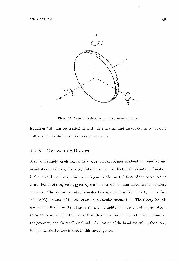
Figure 22: Angular displacements in a symmetrical rotor.
Equation (18) can be treated as a stiffness matrix and assembled into dynamic
stiffness matrix the same way as other elements.
4.4.6 Gyroscopic Rotors
A rotor is simply an element with a large moment of inertia about its diameter and
about its central For a non-rotating rotor, its effect in the equation of motion
is the inertial moments, which is analogous to the inertial force of the concentrated
mass. For a rotating rotor, gyroscopic effects have to be considered in the vibratory
motions. The gyroscopic effect couples two angular displacements (), and if! (see
Figure 22), because of the conservation in angular momentum. The theory for this
gyroscopic effect is in [48, Chapter 8]. Small amplitude vibrations of a symmetrical
rotor are much simpler to analyse than those of an asymmetrical rotor. Because of
the geometry and the small amplitude of vibration of the bandsaw pulley, the theory
for symmetrical rotors is used in this investigation.
CHAPTER 4 47
The inertial moments, Go and G", are
(19)
where D IS the time differential operator, n is the speed of rotation about the
central IT is the second moment of inertia about a diameter and Jr is the
second moment of inertia about the central of the rotor.
Substitute a solution of the form
(20)
into Equation (19), the dynamic stiffness matrix can be obtained as
iJ,flw 1 (21)
The coupling terms involve the first time differential, therefore the dynamic
stiffness matrix is skewed symmetric and the off-diagonal terms are complex. This
fact will impose problems in the search for natural frequencies of a gyroscopic system.
Fortunately, modern computer languages, such as FORTRAN 77, can deal with
complex values and arithmetics easily and efficiently. Section 4.7 will discuss
method of searching for the complex roots of the determinant of the dynamic stiffness
matrix.
4.4.7 Springs
There are two types of springs, linear and torsional. A spring element is considered
to be acting in one direction only. Its effects in any other directions have to be
treated as seperate elements.

CHAPTER 4 48
For a linear spring with U1 and U2 as the end displacements, that is
(22)
The stiffness matrix is
[ kk -kkj [K]spring =. .. (23)
where k is the spring stiffness.
The torsional spring dynamic stiffness matrix is the same as Equation (23) with
k as the torsional spring stiffness.
4.4.8 Dampers
A viscous damper does not have stiffness, however, it has a relationship between
force and displacement, which can be treated as dynamic stiffness. The displacement
vector, {Ii} is the same as {1I} for the spring, and the dynamic stiffness matrix is
given by
[K]damp [
i~c ~iwc j -2WC 'lWC
(24)
where c is the damping constant.
The dynamic stiffness matrix is complex, and can be analysed the same way as
for a gyroscopic rotor. When damping exists, the amplitude of oscillation will decay.
This decaying factor is included in the dynamic stiffness method as an imaginary
part of the frequencies.
The usual notation for the solution, when damping is present, is {Ii} instead
of eiwt {II}, where {Ii} is the amplitude vector, and ,\ is the complex eigenvalues of
the dynamic stiffness matrix. The imaginary part of ,\ is the damped natural fre
quency and the real part represents the decaying part, while the real and imaginary

CHAPTER 4 49
parts of the amplitude together define the amplitude and phase of the vibratory
motion [90]. To be consistent with other dynamic stiffness matrices, eiwt {V} was
used instead. w is also complex but the real part represents the usual frequency and
the imaginary part represents the decay when damping exist, that is A = iw. The
imaginary part is zero when there is no damping in the system .
4.5 Problem with the
Determinants
. e Magnit of the
It is possible for the magnitude of the determinant of the dynamic stiffness matrix
for a beam to be infinite, and sign changes of the determinants could occur at such
infinities.
For a single beam element, the infinities occur at the natural frequencies of
beams with the clamped-clamped boundary conditions, because the stiffness matrix
is undefined for this case as there is zero generalised end displacement. This may
be seen by inspection of the dynamic stiffness matrix for a thin beam, the process
responsible for the infinite magnitudes of the determinant is the division by when
F3 = 0; F3 is the frequency equation for the clamped-clamped bealn. To eliminate
this problem, an extra node is provided where the generalised displacements is non
zero.
For structures with two or more beams, the above problem is much less likely to
happen, however, there are cases when the mode of vibration is such that there are
zero displacements at all the generalised coordinates, and determinantal infinities
are again encountered. An example of this is the third mode of the inplane vibration
of a portal frame as in Figure 23. In this case) an extra node on any member of the
frame will eliminate the problem.

CHAPTER 4 50
Figure 23: Third mode of a portal frame.
At the time of developing the computer program, the determinantal infinities was
avoided by using three node beam elements, that is, an by 18 dynamic stiffness
matrix was obtained for a 3 dimensional beam element instead of a 12 by 12 matrix.
method was acceptable for analysing structures with a small number of beams,
but, the inefficiency of the method was evident when analysing structures with more
than five beam elements. A more efficient way of dealing with this problem would
be to analyse the usual two node beam elements, for a check to be included in
the program to 'detect the possible determinantal infinities and for it to report a
message. An extra node could then be added manually into the structure to remove
the infinities.
4.6 o System and Transformations
The process of assembling the global dynamic stiffness matrix involves two
The first step is the transformation of the dynamic stiffness matrix based on the local

CHAPTER 4 51
y
x
z
Figure 24: Global coordinates in three dimensions.
coordinates system, to the dynamic stiffness matrix based on the global coordinates
system. The second step is the assembly of the transformed elemental dynamic
stiffness matrices into a global dynamic stiffness matrix. This second step, in fact,
imposes compatibility conditions on the model, or in other words, the assembly
process links all the elements together to form the total system representation.
4.6.1 Coordinates System
The global coordinates system (x, y, z) is the coordinates system where the whole
structure is referred to in space. The global degrees of freedom are the degrees of
freedom of all the nodes of the structure in the directions of the global coordinates.
In three dimensional space, each free node has six degrees of freedom, of which,
there are three displacements and three rotations. A completely restraint node has
zero degrees of freedom.
The local coordinates system (X, Y, Z) is the coordinates system defined on each
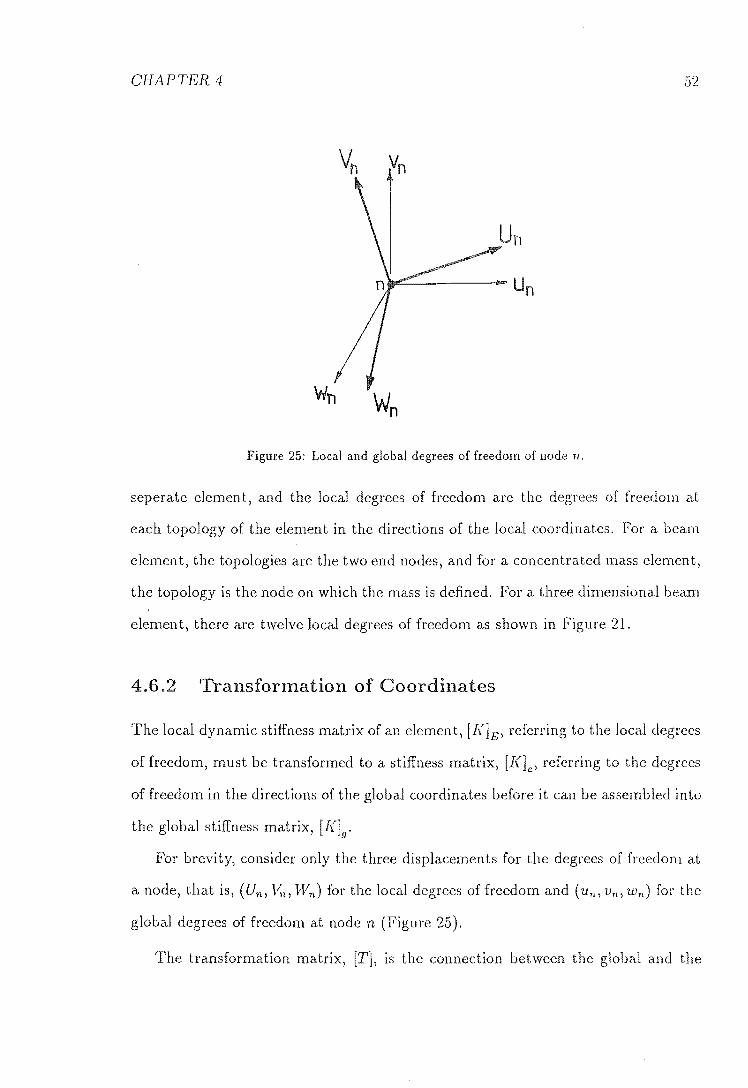
CHAPTER 4
Figure 25: Local and global degrees of freedom of node n.
seperate element, and the local degrees of freedom are the degrees of freedom at
each topology of the element in the directions of the local coordinates. For a beam
element, the topologies are the two end nodes, and for a concentrated mass element,
the topology is the node on which the mass is defined. For a three dimensional beam
element, there are twelve local degrees of freedom as shown in Figure 21.
4.6.2 Transformation of Coordinates
The local dynamic stiffness matrix of an element, [K]El referring to the local degrees
of freedom, must be transformed to a stiffness matrix, [KJe, referring to the degrees
of freedom in the directions of the global coordinates before it can be assembled into
the global stiffness matrix, [K]g.
For brevity, consider only the three displacements for the degrees of freedom at
a node, that is, (Un' 11,1' Wn) for the local degrees of freedom and (un, Vn, 10,,) for the
global degrees of freedom at node n (Figure 25).
The transformation matrix, [Tl, is the connection between the global and the

CHAPTER 4
local coordinates.
[T]
If Un can be written in terms of Un, Vn and 'Wn as
and similarly
then the transformation matrix can be expressed as
Zu Ju ku
[T] = Zv Jv kv
Z11' J11' k-w
53
(25)
(26)
(27)
(28)
(29)
The same [T] can be used to transform the three rotational degrees of freedom,
For a three dimensional beam, the global positions of the two end nodes do not
completely define the position of the beam. One of the methods used by the finite
element scheme to define the local coordinates of a three dimensional beam is the
third node method, where the coordinates of another point lying on the X plane
of beam is provided (Figure 26).
If (Xl,Yl,zd ,(X2,Y2,Z2) and (X3,Y3,Z3) are the global coordinates of node 1,
node 2 and node 3, respectively, and L is the length of the beam, then i u ) ju and
ku are give by
. Y2 - Yl Ju = L
ku (30) L

CHAPTER 4
y
y
z
X-Y plane
x
3 '\
" " \ \
\
" \
z
Figure 26: Third node of a beam element.
x
2

CHAPTER 4 55
iw,jw and kw define a vector perpendicular to the X-Y plane, hence
(iw,jw,kw) - (iu,ju,ku) X X3 Xl Y3 - Yl Z3 - Zl)
L3 ' L3 ' L3 (31)
where
Similarly, iv,jv and kv define a vector perpendiculaT to the X-Z plane, therefore
(iv,jv,kv) - (iu,ju,ku) X (iw,jw,kw ) (32)
The stiffness matrix, [K]E can be transformed to [Kle by [48, page 72],[14, page
151]
[Kle = [Tf (K]E [T] (33)
4.6.3 Assemblying the Global Stiffness Matrix
The assembly process is merely the additions of the elements of the matrix [Kle
to the appropriate ro\vs and columns of the global matrix [K]gl depending on the
numbering scheme of the global degrees of freedom. More information on this process
can be found in most FEM text books, such as [14].
4.7 Roots Finding Method
This step is very important in the analysis and probably the most difficult step.
For FEM, solution of the frequency equation of a system is a linear eigenvalue
problem. All the eigenvalues can be found by a nUIIlerical algorithm [74]. The
number of eigenvalues obtained is dependent on how many elements were chosen to
approximate the problem.
With the dynamic stiffness method for a beam, solution of the frequency equa-
tion is a transcendental eigenvalue problem, hence there are an infinite number of

CHAPTER 4 56
x· I X I
x x
Figure 27: Secant's and Muller's methods.
frequencies, which is expected because there are infinite degrees of freedom. The
only way to find the roots of a transcendental equation is to search for each fre-
quency with a robust numerical scheme. Bisection method, regula falsi method,
Secant method and Newton-Raphson method are a few popular methods for find
ing roots of a general equation. Williams and Wittrick [92] described an infallible
method of finding all required natural frequencies of skeletal structures. However,
these methods are for real roots only. There are very few methods that can handle
complex equations and complex roots.
Text books on Numerical Analysis [63,13] suggested the Muller's method as a
robust numerical algorithm for finding real and complex roots of a general equation.
Muller's method works on the same principle as the Secant method, but instead
of using linear interpolation, Muller's method uses quadratic interpolation to find
the next approximate point (Figure 27)
To find a root of a function F (x), Muller's method requires three initial guesses,
Xi-'l, Xi-I, Xi. Then the next approximation Xi+l can be found as followed
q =

CHAPTER 4
A qF (Xi) q (1 + q) F (xi-d + q2 F (Xi-2)
B (2q+1)F(xi) (1+q)2F(xi_d+lF(xi_2)
c (l+q)F(xi)
Xi - (X i-X i -1) [-=B--:--r2:::::=;:C======:= 1 yB2_4AC
57
The sign in the denominator of the above equation is chosen to make its value
as large as possible.
Because of the square root in the equation, a complex value for Xi+l is possible
hence the method can converge to a complex root.
The Muller's method is believed to have almost global convergence, that is, it will
converge to a root with any starting values. However, it is impossible to establish
which particular root the method will converge to, hence some roots may be missed
during a search.
The Muller's method was adequate for providing the solutions of this analysis.
The mode shapes were plotted to check the validity of the roots found.
The algorithm given in [13, page 72] is more efficient and more stable than the
above algorithm. It is
hI xi-l - Xi-2
h2 Xi - Xi-l
F al
F ') / a2
d a2 - a]
h2 + hI
b a2 + h2d
D Jb2 - 4F (Xi) d
2F Xi+! X--,
b±D

CHAPTER 4
A computer subroutine based on algorithm was written in FORTRAN
it was used to find the natural frequencies of the bandsaw structure.
.8 escription t er Program
A program to analyse two diIl1ensional structural vibrations, VIB2, was written first
to examine the practicability of the dynamic stiffness method, and also to provide
test results for the full three dimensional vibration problems. Only transverse and
longitudinal vibrations of thin beams were considered in VIB2.
VIB~3 was written as a general computer to analyse the vibrations of
dimensional structures consisting of thick beams, masses, springs, dampers
and gyroscopic rotors.
4.8.1 Hierarchical Structure of VIB3
The program reads input data from a data file which fully defines the vibratory
Three main tasks of the program are:
• To find the values of the determinant of the dynamic stiffness matrix for a
given range of frequencies and step size.
find the natural frequencies of the system by using Muller's method to
for the roots of the function F(w), where w is the angular natural
frequency and F (w) returns the value of determinant of the dynamic stiffness
matrix. The three initial starting points affect which frequencies the method
will to, therefore care must be taken to find all required natural
frequencies.

CHAPTER 4 59
iI9 To plot the mode shapes of the system at a gIven natural frequency. The
task of visualising the mode shapes is as important as the task of finding
the natural frequencies. There is a considerable amount of work involved in
generating the mode shapes of complicated structures by hand. Fortunately,
computer graphics can be used to automate this process.
Figure 28 shows the hierarchical structure of VIB3. The program is menu-driven
to give the users more flexibility.
4.8.2 Input Data
The preparation of input data for VIB3 was designed to be similar to the input for
PAFEC, the commercial finite element software.
VIB3 data is in modular form, each module begins with a header, hence the
module can be placed in any order. There are eight modules available
MATERIAL defines the material and geometrical properties of the beams. Each
set of properties is numbered so that it can be referred to in the program.
Because of the complexity of calculating the geometrical properties of various
cross sectional shapes (rectangular, I section, T section etc.), especially the
shear coefficients [15], and the torsion constants [67], a computer program,
PROP, was written to calculate all the geometrical properties of various cross
sectional geometries.
NODE defines the coordinates of all the nodes of the structure.
BEAM defines the topologies of the beams, directions of their principal planes,
and the connections at their ends. At the moment, VIB3 considers only the
rigid joints and the pinned joints, but elastic linkages can be included at a
later stage [61].

CHAPTER 4 GO
I Read Da ta J
I Define Global d.o.f. I
. I D ERMI NANTS :
Determinant of Stlf fness Matrix
I FREQUENCIES i Stiffness Matrix
Transformation of
I ( 0 0 rd ina t e s
•
I MODE SHAPE I I
Beam r-
End Displacements I ----1 Mass H
• I Rotor Shape of Beams
~ I Spring
Plots1 Oa mper I
~ ~ t ~ t I Undeformed I I Deformed I ITraceOfl I
I I S true ture Structure Nodes
Figure 28: Hierachical structure of the program.

CHAPTER 4 61
RESTRAINT defines the global boundary conditions.
MASS, ROTOR, SPRING and are modules which define the prop-
erties and the topologies of the concentrated masses, gyroscopic rotors, linear
springs, torsional springs, linear dampers and torsional dampers. The modules
can be omitted if the elements are not in the structure.
4.8.3 Output data
The output data is stored in a file and displayed on the screen.
The DETERMINANT option asks for a range of frequencies and the step size,
then displays the frequencies with their corresponding values of the determinant of
the stiffness nutrix. Sign changes can be detected by visual inspection. This option
can be used to give an indication of the location of natural frequencies. However,
when the determinant has complex values as for the cases when gyroscopic rotors
are included, it is impossible to infer the natural frequencies by visual
inspection.
FREQUENCIES option requires three starting values for the iteration, then
uses Muller's method to search for a natural frequency. It is not possible to know
which frequency the method will converge to, but usually it will converge to the
roots closest to the three starting points.
Once a natural frequency has been detected, the MODE SHAPE option can
be used to plot the mode shape. The program uses P LOT79 graphics package to
generate three views of the structure and its mode of vibration. One isometric
view of the structure gives the overall picture of the vibratory mode, however, it
can be ambiguous, therefore, a plan and an elevation views are plotted to define it
unambiguously.

C apter 5
E PERIME TAL RESULTS
AND THEORETICAL
E PLANATIO S OF TH
WAIMAK BANDSAW
VIBRATIONS
5 .1 Introduction
About ten years ago, the Waimak bandsaw was reported as having problems with
excessive vibration. Attempts to reduce the vibration, such as rebalancing the pul
leys and bracing the structure to the ground, were unsuccessful. About a year ago,
during a maintenance overhaul, one of the rolling contact bearings was found to be
defective and was replaced. This appeared to reduce the vibration to an acceptable
level, when the bracing was removed.
62

CHAPTER 5 63
Although, this bandsaw had no vibration problem at the time of the experiments,
problems have been reported on similar bandsaws in other saw mills in New Zealand.
Also a better understanding of the vibrational characteristics of the Waimak band
saw may help to explain the reasons for some of the vibration problems occurring
on the other bandsaws.
The steps involved in the experiments and in the interpretations of results were
not straight forward. The experimental anlysis had to be carried out in conjunction
with the theoretical analysis, to explain the modes of vibration of the Waimak
bandsaw.
The bandsaw structure was broken up into three sections as described in Chap
ter 2, and the assumption made was that the vibrations of these sections were
uncoupled from each other, that is, each section could be analysed independently.
5.2 The Base
The base of the bandsaw is essentially a short cantilevered plate with masses at
tached to it. The programme VIB3 does not consider the plate model, but from
practical intuition, the base is expected to be reasonably stiff compared with the
other parts of the bandsaw.
The response of the base to an impact showed many peaks in the frequency
spectrum. Some of the low amplitude peaks in the spectrum were related to the
natural frequencies of other sections of the saw. By exciting and measuring the
responses at different locations on the base, it was found that 168 Hz and 195 Hz
were the dominant natural frequencies of the base. The 168 Hz had been identified
as a transverse mode and the 195 Hz was a transverse-torsional mode, as shown
in Figure 29. The coupling in the 195 Hz mode was due to the mass of the main
column being situated on one side of the base, therefore it coupled the transverse

CHAPTER 5 64
168 Hz 195 Hz
Figure 29: Mode shapes of the base.
mode with the torsional mode.
Although these results showed that the base was not rigid, its natural frequencies
were high compared with the natural frequencies of the other sections, therefore, it
was reasonable to assume that the dynamics of the section below the base would
have very little influence on the dynamics of the section above it in the low frequency
and vice versa.
5.3 Section elow the ase
This section was quite simple compared with the section above the base. Its ba
sic components were the bottom pulley, the shaft and the brackets supporting the
bearing housings (Figure 30).
5.3.1 Experimental Results and Interpretations
Figure 31 shows the spectrum of an accelerometer reading, which was placed on the
bearing housing in the axial direction of the shaft.
Three natural frequencies shown in the spectrum were approximately 30 Hz,

CHAPTER 5
>, . .:':..
6W-1
1-..... .
('~.'
::'l "I"~
-:1>
Base
Bracket
1~~:""-:-=-'-:!""'-8earing .,: 1',- j
Housing ,~'
af t ,~,~'I:""", >::':: .\.: '., .... ,,-..r • .,......
... .1'\ ~. .
?ulle y, _:: ,: "t~""""---'-:~
Figure 30: Section below the base,
FNl...LlG IN 69 09 19 17 [X) 42 RVERRGEft LINEAR SP YR= 43.213m XR= 36.5000 0915172926 LINEAR SP YB= 38. 940m XB= 30.0000 0915172926
3CO.COm-t------'--,--,-'-----"'----'-----mm. . I • .---'--- r R CHI PYR= 216. !
REAL PXR= 152. r xl r
ESD
B CHI REAL
Xl ESD
o
r
r i r
Figure 31: Frequency spectrum of a response of the section below the base,
65
I •
,\ .. , . 1 ' --I'
,"'~., -

CHAPTER 5 66
36 Hz and 152 Hz.
The shaft alone would have had quite high natural frequencies, but the inertia
of the pulley reduced the shaft frequencies considerably. This was analogous to a
cantilever beam with a concentrated mass attached at the end.
The phases between two accelerometer readings at various positions on the rim
of the bottom pulley revealed that the 30 Hz frequency was related to the first
transverse mode of the shaft in the horizontal direction, the 36 Hz was related to
the first transverse mode of the shaft in the vertical direction, and the 152 Hz was
the swinging mode in the axial direction of the shaft. There were 90 Hz and 95 Hz
natural frequencies present in the measurements on the rim of the pulley, however,
their mode shapes were not identified during the experiments.
5.3.2 Theoretical Analysis
The programme VIB3 was used to obtain the first few natural frequencies and mode
shapes of the section below the base of the bandsaw.
The model consisted of four beams and a rotor. The model mesh is shown in
Figure 32.
It was assumed that the material properties for both the shaft and the brackets
were those of mild steel, this was a reasonable assumption because the variations in
the properties of different types of steel were small.
The plots of the first five modes are in Figures 33,34,35,36, and 37.
Although the natural frequencies differed from those obtained experimentally,
the first, second and fifth mode shapes agreed with those found experimentally. The
shapes of the third and fourth mode were identified as the second transverse modes
of the shaft in the horizontal and vertical directions, respectively. They appeared to
be the mode shapes of the 90 Hz and 95 Hz natural frequencies in the experiments.

CHAPTER 5
1
2~-------------+~--~4 3
Figure 32: Model mesh.
x -z PU,N[
PLOT OF DISPLACEMENTS fRE(HZ)= TI~1E
25.5 0.0
VI :3 REf. DATE
WAI;.IK5 2J-JAN-90
Figure 33: First mode.
67

CHAPTER 5
PLOT OF DISPLACEMENTS
VIE3
PLOT OF DISPLACEMENTS
VIE3
fRE(Hz)= TIME REF. DATE
J7.4 0.0
WAIUK5 2J-JAN-90
Figure 34: Second mode.
fRE(Hz)= TIME REF. DATE
57.7 0.0
WAIUK5 2J-JAN-90
Figure 35: Third mode.
68
x-z PLANE
..... - - -
Y-Z PLANE
X-Z PLANE
Y-Z PLANE

CHAPTER 5
PLOT OF DISPLACEMENTS
VIB3
PLOT OF DISPLACEMENTS
VI
fRE(Hz)= TIME
REf. DATE
69.3 0.0
WAIMK5 23-JAN-90
Figure 36: Fourth mode.
fRE(Hz)= TIME
REf. DATE
102.1 0.0
WAIMK5 23-JAN-90
Figure 37: Fifth mode.
69
x-z PLANE
x-z PLANE
Y-Z PLANE

CHAPTER 5
Shaft
Column Slide
\
I
I I
I
Pulley
Main Column
Figure 38: Main components of the section above the base.
5. Section Above the ase
70
As previously mentioned, this section of the bandsaw is far more complicated than
a simple beam-structure. The programme VIB3 was, therefore, used only to explain
some of the natural modes of the structure, the calculated natural frequencies were
not expected to be close to the measured natural frequencies.
The main structural components of this section were the main column, the col-
umn slides, the top shaft, and the top pulley. Figure 38 simplifies the section above
the base to only the main components of interest.

CHAPTER 5
5.4.1
WR I VA< - ;26-6-88 FN=LOO IN
LINEAR SP 10.
R CH2 REAL
Xl ESO
o
EX 2-A ACe 10 000927 163323 ~5 ,
-m-a 5. ma7rn XRoo 9. ()(J[)(XJ D92'7163213
Pyf'F> 6. 42.35m ~ 132.50
Figure 39: Frequency spectrum of the side-to-side transverse vibration.
Experimental Results
71
Frequency response functions were obtained for vanous positions of measurement
and of excitation. These results were similar to those obtained from the frequency
spectra of the transient response. This meant that the one parameter reading
method was acceptable as the measurement method for these experiments. Fig-
ure 39 and Figure 40 show the frequency spectrum and the frequency response
function measured on the left bearing housing in the axial direction of the shaft.
These plots show that the major natural frequencies, in the side to side vibra-
tions, were the 9 Hz, 135 Hz, 260 Hz.
Figure 41 and Figure 42 show the frequency spectrum and the frequency response
function measured in the to-and-fro transverse direction. These two graphs indicated
that 21 Hz, 96 Hz and 157 Hz were the natural frequencies of the structure.
It was assumed that the stiffness of the column slides would not alter the flexural
rigidity of the main column, because they were not rigidly attached to each other.
I-Ience, the column slides were treated as masses only, which were attached to the

CHAPTER 5
WRIMRK - 26-8-88 F-l-l ANALOG IN 88 09 Z7 09 RVERFlGE#
TRRNS FNC YA=: 5. 2872mXR= 8. f"?LC(""'\(""'\(""'\ 0826150944
6O.000m-h--~--~~-r~--~--~----L---~~~--~--~+
MRG
Xl
o
CH2
o Xl LIN Hz
13.729m 135.00
500.00
Figure 40: Frequency response function of the side-to-side transverse vibraLion.
~IMAK - 26-8-86 EX 2:-e: Fa: 9
L~ ~ 'l'FP 6.1~ 10. DOOm
R Di2 REAL
Xl E.SD
o
1.7~D4 95.0000 1.1
Figure 41: Frequency spectrum of the to-and-fro transverse vibration.
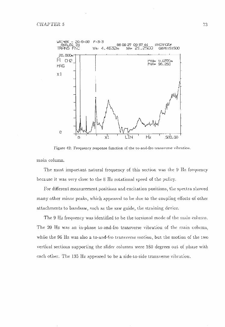
CHAPTER 5
WRIMRK - 26-8-88 F-3-3 RN=lLClG IN B8 09 'Z7 09 S7 44 RVERAGEif
TRRNS FNC YR= 4.4632m XR= 21.2500 0826151500
2O.CDJm
R CH2 MAG
Xl
o
PYR= 9.037On PXR= 96.250
Figure 42: Frequency response function of the to-and-fro transverse vibration.
main column.
73
The most important natural frequency of this section was the 9 Hz frequency
because it was very close to the 8 Hz rotational of the pulley.
For different measurement positions and excitation positions, the spectra showed
other minor peaks, which appeared to be due to the coupling effects of other
at tachments to bandsaw, such as the saw guide, the straining device.
The 9 Hz frequency was identified to be the torsional mode of the main column.
The 20 Hz was an in-phase to-and-fro transverse vibration of the n column,
while the 96 Hz was also a to-and-fro transverse motion, but the motion of the two
vertical supporting the slider columns were 180 degrees out of phase with
each other. The 135 Hz appeared to be a side-to-side transverse vibration.

CHAPTER 5
A A
. , " \
::. -
II . \
\ . • I , \ \ "'" ....
.) ~-... ;: "" ..
ieal Stiffener
1
Figure 43: Main column.
5.4.2 Theoretical Analysis
74
A natural frequency of 9 Hz was very low for this structure, which meant that there
was a very flexible component in the structure. Some considerations on the possi-
ble causes of this low natural frequency, by theoretical and experimental analyses)
concluded that the most likely cause of this 9 Hz was the torsional vibration of the
main column.
The main column consisted of two beams extending 1.5 m from the base, and
a plate, which was welded between the two beams at about 0.5 111 above the base,
leaving 1 m free length on the beams (Figure 43). two beams could be
considered as tapered-I sections. The web thickness was only about .016 m.
As a preliminary test of the validity of the hypothesis of low torsional stiffness,

CHAPTER 5
Mass
I t,.../
\
" /
\
\
\ \
\ \ \ \
\
1
)
Figure 44: First model mesh.
75
a simple model of the main column was investigated. This simple model considered
only one beam section of the main column. The mass of one slider column and half
the mass of the top pulley was represen ted as a concen tr ated mass (Figure 44).
Figure 45,46, and 47 show the first three modes of this simple model. The first
mode was, as expected, the torsional mode of the vertical beam, and the natural
frequency was also very low. The second mode also matched with the second mode
in the experiments, that is, the to-and-fro transverse mode. The 96 Hz obviously
could not have been predicted by this model, because it would have required two
beams to model the main column. The third mode in the theoretical analysis agreed
with the 135 Hz in the experiments.
A more complete model of the structure was then analyzed, which took into
account the whole structure of the main column and the inertia of the top pul-
ley. The model mesh is shown in Figure 48 and the first five mode shapes are in
Figures 49,50,51,52 and 53.
The first mode shape was agam the torsional mode of the main column, and

CHAPTER 5
,
\~I
- ---
~LOT OF DISPLACEMENTS fRE(Hz)= 5.1 TIIAE = 0.0
VIB3 REf. : WAIMK6 DATE : 23-JAN-90
Figure 45: First mode shape of the first model.
" , , ,
,
, I
I
.•• _-' •• ---3
PLOT OF' DISPLACEMENTS fRE(Hz)= TI~IE =
VI REf. : DATE :
4B.7 0.0
WAIMK6 23-JAN-90
Figure 46: Second mode shape of the flrst model.
76
_0 --- ---- .
X-Z PLANE
Y-Z PLArJ[
X-Z PLANE
I --I
... I
I I
I
Ii
Y-Z PLANE

CIlAPTEH 5
\
\~I
- - --L - -- -
If
x -2 PLANE
PLOT OF DISPLACEMENTS fRE(Hz)= 57.4 TIME = 0,0
VIl33 REf. : WAIUK6 DATE : 2J-JAN-90 Y-Z PLANE
Figure 47: Third mode shape of the first modeL
~---',
",'1 \ '" I \
I
.. 1 , I
'/~Rotor
Figure 48: Second model mesh.

CHAPTER 5 78
\
\~l
~ \ \
\ \
\ \
\ \
\j \ \
---- X -Z PLANE
PLOT OF DISPLACEMENTS FRE(Hz)= 4.9 TIME = 0.0
VIE3 REF. : WAllAK7 DATE : 29-JAN-90 Y-Z PLANE _ ......
Figure 49: First mode shape of the second model.
\
\~l '1
~--\
I \
\ \
\ \ I I 1\' I \ ..
~U X-Z PLANE
\ I
I I I
I
PLOT 0 F DISPLACEMENTS FRE(Hz)= 30.6 TI).~ E = 0.0
VIE REF. : WAIIJK7 DATE : 29-JAN-90 Y-Z PLANE
Figure 50: Second mode shape of the second model.

CHAPTER 5 79
,
\~l
\ \
\
\
~~ --- -- \
\ I
0; I .,-.;:--"'"
I ~ I ~
~
I ~ ~
V or X-Z PLANE
-.1.-' --
.:
PLOT OF DISPLACEMENTS fRE(Hl)= 40.5 TIME = 0.0
VI133 REF. : WAII.4K7
I DATE : l-FEB-90 Y-Z PLANE
Figure 51: Third mode shape of the second model.
, \~l
( I
~ -- I
I I - ,-._ .. I
-I I
"-- - I - --I--- I
r--- X-Z PLAN~----
-- --I--~ --.
PLOT OF DISPLACEMENTS FRE(Hz)= 55.1 TIME = 0.0
VI133 REF. : WAII.4K7 DATE : 29-JAN-90 Y-Z PLANE
52: Fourth mode shape of the second model.

CHAPTER 5 80
\
,~\ I
~-\
\
\
\
\} \
-
----- X-Z PLANE
-
I I
I I
I
PLOT OF DISPLACEMENTS FRE(Hz)= 104.6
·TIME = 0.0
VII33 REF. : WAIMK7 DATE : 29-JAN-90 Y-Z PLANE
Figure 53: Fifth mode shape of the second model.
the associated natural frequency was 4.9 Hz. This mode shape was a very close
representation of the 9 Hz measured natural frequency. The next natural frequency
was at 30.6 Hz, which was a combination of the torsional mode on one vertical
beam of the main column, and the transverse mode on the other. The third natural
frequency was 40.5 Hz, with a coupled transverse-torsional mode. This mode shape
appeared to match that of the measured 96 Hz natural frequency. The first to-and-
fro transverse mode was at 55.1 Hz natural frequency, which related to the measured
21 Hz frequency. The fifth mode was the side-to-side transverse mode at 104.6 Hz
frequency. The measured natural frequency for this mode was 136 Hz.
The theoretical model predicted all the modes of vibration observed on the
\Vaimak bandsaw, and suggested one other, which was not realised at the time
of the experiments. Although the third and fourth mode shapes were found in
the experiments, their associated natural frequencies were quite different to those

CHAPTER 5
WT-2 FN=l...CG IN
TRANS FNC TRANS FNC 8.0000 -t-~
R CH2 i MAG l
I
Xl
B CH2~ I'1RG l xl
o
6909 19 162446 ~ Y"R- 686.28m )(R.s 5.75000 0915165023 YB- 907. 86m xe- 1. 10000 0915165023
.. xl
J L1N
~-r f"(A.s 4. 5B5O ~ 3.B250 r
I
r
r
r r
Figure 54: Frequency response function of the straining device, 0-10 Hz.
obtained experimentally.
5.5 Straining Device
81
The components of the straining device include the counterweight, the lever arm,
the fulcrum shaft, and two compression rods. Figure 10 in Chapter 2 showed the
assembly of a counterweight mechanism.
5.5.1 Experimental results
There was a low natural frequency, which related to the rigid body motion of the
straining mechanism, that is, the vertical motion of the two top bearings. The
stiffness was provided from the longitudinal stiffness of the saw blade, and the mass
was a combination of the mass of the top pulley and the counterweight. Figure 54
showed that this oscillation was at 3.8 Hz and the width of the peak was very narrow
which meant that there was little damping in the oscillation.

CHAPTER 5 82
WT-l' f'ClW<llr 5pecirurn FN=l....ClG IN 00 09 19 1816 58 ~
RUTCl PW SF 'l"R- 198. 36u. XR= 31. 0000 0915163'702 AUTCl PW SF YB- 1. 02S76m )(&.. 1.75000 0915163'702
3. 0000m crVF;S1: ~-- r R D--I2 _ F"Y'"R- 343.:32u REAL f>XR= 47.500 r
-Xl
E5D - r --
B D--I2 -
REAL. -
Xl E5D
0 \. -0
Figure 55: Frequency spectrum of the straining device, 0-100 Hz.
Figure 55 and Figure 56 show a frequency spectrum and a plot of the frequency
response function of the vertical motion of the bearing housing for a range 0-100 Hz
frequency. These two plots agreed that 31 Hz, 48 Hz, 87 Hz were the three dominant
natural frequencies of the mechanism.
These vertical vibrations of the bearings would produce tension fluctuations in
the saw blade, especially at 3.8 Hz because of large displacements. Other frequencies
were also of interest because it was possible for the blade to become unstable at
certain frequencies due to parametric excitation, as will be discussed in Chapter 10.
5.5.2 Theoretical Analysis
The low frequency vertical oscillation of the top pulley could be modelled accurately
by representing the structure of the straining mechanism as a simple spring-mass
system. The fulcrum shaft, the two compression rods and the top shaft could be
assumed to be rigid for this low frequency oscillation, hence could be removed from
the model. This assumption reduced the system to two masses and a spring as in

CHAPTER 5
WT-l Tl"w .... i<1l.l" Func t (an A\A....ClG IN
TRANS FNC YA-TRANS FNC ya... 3O.000m~--~--~~--4r--~--~----~-.~--~--r-~--·
R CH2 /VAG
Xl
B D-i2 /VAG
Xl
o
Figure 56: Frequency response function of the straining
r
r
r
00
0-100 Hz.
83
Figure 57. Mass 1111 was the mass of the counterweight (85 kg), mass m2 was the mass
of the top pulley, the shaft, the bearings and the bearing housings (approximately
600kg), and the spring stiffness could be approximated from the longitudinal stiffness
of the non-cutting and cutting spans of the blade, k ,·where was the Young's
modulus, A was the cross-sectional area of the blade and L was the length of the
blade, and for this case
k = 2 x 200 X 109
x 0.22 x 0.00165 _ 63.4 x 10⁶ N /m 2.29
The natural frequency of the system, w, was given as
k w= (34)
For the Vvaimak bandsaw, ~ = 42, hence w = 20.5 rad/s, or 3.3 Hz. This was
very close to the measured frequency of 3.8 Hz.
This analysis showed that the 3.8 Hz frequency of oscillation could be altered
by choosing appropriate magnification ratio of the lever arm, %, and the mass of

CHAPTER 5 84
a b
~ J\
0
m, k
/ II II
Figure 57: Model to represent the rigid body mode of the straining device.
the counterweight, mI. For example, if ~ was reduced to 21 instead of 42, then
1nl has to be 170 kg instead of 85 kg to produce the same amount of strain on the
saw blade, and the natural frequency becomes 4.6 Hz instead of 3.3 Hz. Although
this oscillation of the counterweight had not been under any investigation, it was
possible that shifting the natural frequency could improve the cutting performance
of the saw blade, and this could be achieved by a simple alteration to the existing
bandsaw.
The other frequencies that appeared in the spectrum were related to the struc
tural vibrations of the components in the mechanism. The programme VIB3 showed
that the dynamics of the components of the straining mechanism were uncoupled,
hence they could be considered individually.
For the lever arm, the calculated first natural frequency in the vertical direction
was found to be 226 Hz (by considering it as a pinned-free beam with a mass at
the free end). The first frequency of the lever arm in the horizontal direction was
only about 4 Hz, however, this vibration would not affect the vertical motion of the
bearings.
The torsional and transverse vibrations of the fulcrum shaft were also considered
as possible causes of the vertical vibrations of the bearings. It was difficult to

CHAPTER 5 85
establish the end conditions for the fulcrum shaft, but for various combinations of
the end conditions, the first torsional frequency seemed to be always greater than
150 Hz. The calculated first transverse frequency of the fulcrum shaft was 196 Hz.
A simply-supported beam under constant longitudinal compression was used to
model the transverse vibration of the strain bar, and the calculated first natural fre
quency was 88 Hz. The longitudinal vibration of the strain bar was also considered,
however) the calculated first frequency was found to be greater than 120 Hz.
These considerations only explained the 87 Hz frequency in the experimental
spectrum as the the first transverse frequency of the strain bar. At this stage, the
cause of the 31 Hz and 48 have not been found. However, the vibration of the
column slide in the vertical direction, the connections between the bearing housings
and the column slides, and the connection between the lever arm and the fulcrum
shaft are suspected to be the possible causes of the 31 Hz and the 47 Hz frequencies.
5.6 Theoretical Study of the Gyroscopic Effects
on Bandsaw Structure
Gyroscopic motion has always been a very interesting subject in the field of dynam
ics, and its effects are important in considerating the design of rotating machinery.
In structural vibration problems, gyroscopic effects can couple flexural modes of
vibration and alter the natural frequencies of the system.
The bandsaw consists of two gyroscopic systems; the top pulley and the bottom
pulley. The previous sections have considered the structural natural frequencies of
the vVaimak bandsaw when both pulleys were stationary. Under idling condition,
the gyroscopic effects of the pulleys on the structure may alter the vibrational char
acteristics of the bandsaw, hence they must be examined. The programme VIB3
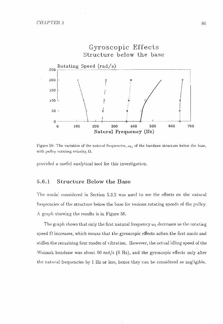
CHAPTER 5
Gyrosco IC Effects Structure below the base
Rotating Speed (rad/s) 250,-----~~~----~--~---·············· ----------------------,
200 \ T " \ 150
\ I
100 t ~
50 + lit \ \
0 0 100 200 300 400 500 600 700
Natural Frequency (Hz)
86
Figure 58: The variation of the natural frequencies, Wi, of the bandsaw structure below the base,
with pulley rotating velocity, n.
provided a useful analytical tool for this investigation.
5.6.1 Structure Below the Base
The model considered in Section 5.3.2 was used to see the effects on the natural
frequencies of the structure below the base for various rotating speeds of the pulley.
A graph showing the results is in Figure 58.
The graph shows that only the first natural frequency WI decreases as the rotating
speed n increases, which means that the gyroscopic effects soften the first mode and
stiffen the remaining four modes of vibration. However, the actual idling speed of the
Waimak bandsaw was about 50 rad/s (8 Hz), and the gyroscopic effects only alter
the natural frequencies by 1 Hz or less, hence they can be considered as negligible.

CHAPTER 5 87
5.6 Structure Above
The main flexural component of the structure below the base was the shaft, which
was parallel to the axis of rotation of the pulley. For the structure above the base,
the main column was the main flexural component and was perpendicular to the
axis of rotation of the top pulley. The behaviour of the structure above the base due
to the rotating pulley was, therefore, expected to be different from the behaviour
described in the previous section.
Figure 59 shows the of varying the rotating speed on the natural frequen-
cies of the second model in Section 5.4.2. The second, third fourth natural
frequencies decreased as the rotating speed increased, the first natural frequency re
mained the same, and the fifth natural frequency increased as the speed increased.
The rotating pulley did not affect the first mode because its motions did not pro
duce any rotation of the spin axis about another axis, hence there was no gyroscopic
coupling effect.
Again, at 50 rad/ s rotating speed, the gyroscopic effects were very small, shifting
the natural frequencies by less than 1 Hz.
5.7
brat
al Results of t
of Bandsaw ...................
tructural Vi
Conditions
The vibrations of the Waimak bandsaw during idling were measured to provide
information about the nature of the bandsaw under normal operating condition.
Only the top section of the bandsaw was considered in the experiment.
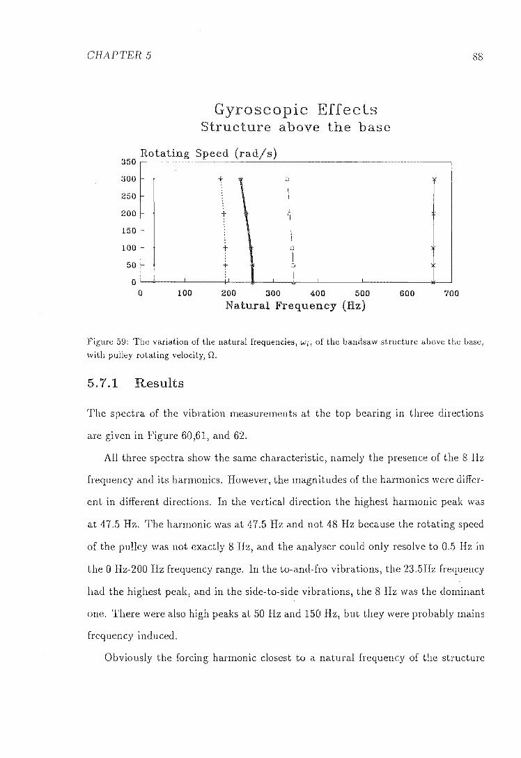
CHAPTER 5
OSCOplC Effects Structure above the base
Rotating Speed (rad/s) 350r-~-~~~~~~~~~~~~~~~~~~~~~··························· ............ -~~.
300 f- t , 250
200 f- ~
150
100 - t 0 I
50 i o I
.i-t :,
I
0 100 200 300 400 500 600 700
Natural Frequency (Hz)
88
Figure 59: The variation of the natural frequencies, Wi, of the bandsaw structure above the base,
with pulley rotating velocity, n.
5.7.1 Results
The spectra of the vibration measurements at the top bearing in three directions
are given in Figure 60,61, and 62.
All three spectra show the same characteristic, namely the presence of the 8 Hz
frequency and its harmonics. However, the magnitudes of the harmonics were differ-
ent in different directions. In the vertical direction the highest harmonic peak was
at 47.5 Hz. The harmonic was at 47.5 Hz and not 48 Hz because the rotating speed
of the pulley was not exactly 8 Hz, and the analyser could only resolve to 0.5 Hz in
the 0 Hz-200 Hz frequency range. In the to-and-fro vibrations, the 23.5Hz frequency
had the highest peak, and in the side-to-side vibrations, the 8 Hz was the dominant
one. There were also high peaks at 50 Hz and 150 Hz, but they were probably mains
frequency induced.
Obviously the forcing harmonic closest to a natural frequency of the structure
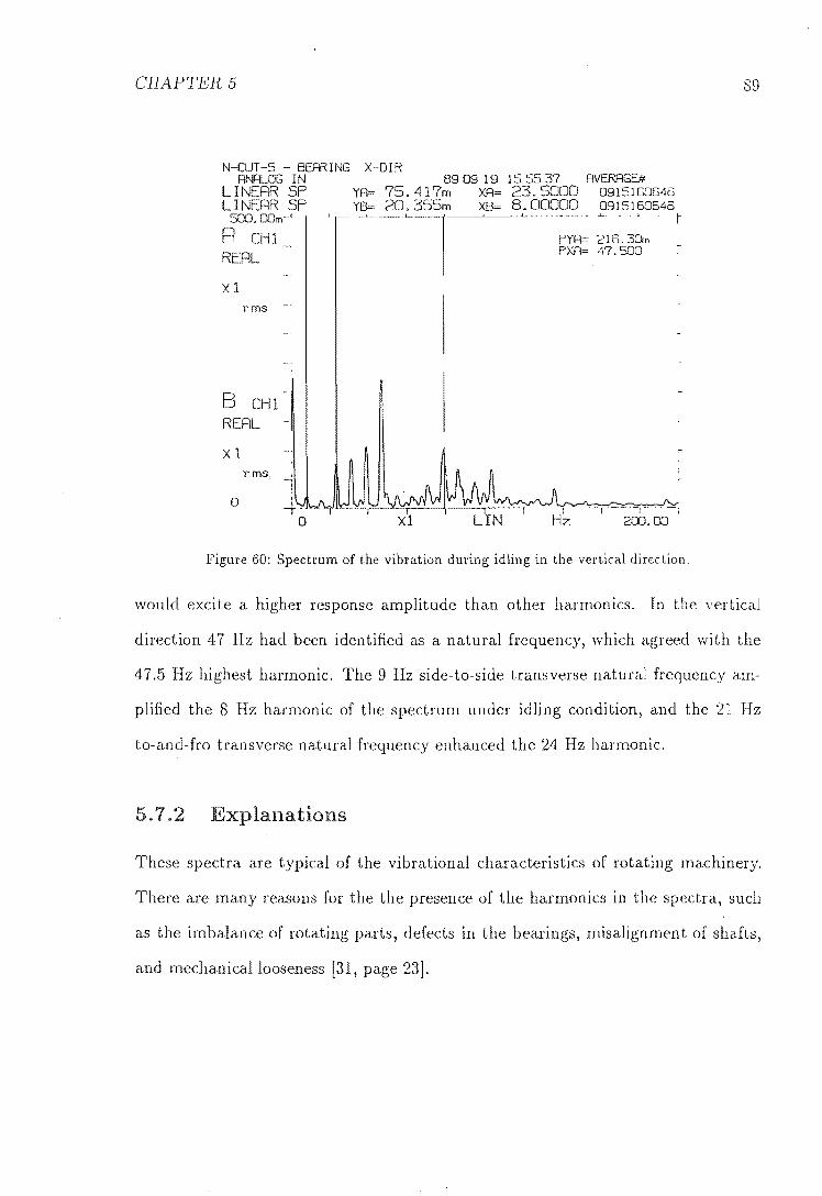
CHAPTER 5
N-CUT-S ING X-DrR RNRLClG
LINERR LINERR SP
5OO.DOm-'
R CHI RERL
xl rms
CHl
Xl rms.
o o
89 09 19 15 55 37 RVERRGE# XA= 23.5000 0915160646 XB= 8.00000 0915160646
--~ .. L---'-"--r--~- L' r
xl
PYR= 216. 30m PXR= 47. SOD
~-~l··-·-··-l-·
Hz 2m. DO
Figure 60: Spectrum of the vibration during idling in the vertical direction,
89
would excite a higher response amplitude than other harmonics. In the vertical
direction 47Hz had been identified as a natural frequency, which agreed with the
47.5 highest harmonic. The 9 Hz side-to-side transverse natural frequency am-
plified the 8 Hz harmonic of the spectrum under idling condition, and the 21 Hz
to-and-fro transverse natural frequency enhanced the 24 Hz harmonic.
5.7 Explanations
spectra are typical of the vibrational characteristics of rotating machinery.
are many reasons for the the presence of the harmonics in the spectra, such
as the imbalance of rotating parts, defects in the bearings, misalignment of shafts,
and mechanical looseness [31, page 23].

CHAPTER 5
N-OJT -6 - BEF«] NG Z -01 R Rl\AU'JG IN
LINEAR SP LINEAR SP
500.00m-'-
R CHl REAL
xl rms
B CHl REAL
xl rms
o
89 09 19 16 00 50 RVERRGE# • 426m XR= 31.0000 0915160921 • 085m XB= 8. 00000 0915160921
PYR= 411. 47m PXR= 23.500
r
I r 200.00
Figure 61: Spectrum of the vibration during idling in the to-and-fro direction.
N-CUT-3 ANALOG
LINEAR LINEAR 5OO.00m~
R CHl J REAL !
Xl rms
I CHll
REAL -j
Xl rms
o
Y-DIR 89 09 19 15 4 1 54 RVERRGE.#
YR= 52. 292m XR= 23.5000 0915160041 YB= 244. 38m XB= 8,00000 0915160041 '~ __ ~ __ --L-_~-'_" >.. , , :--
I06.9Em 31.500
r
Figure 62: Spectrum of the vibration during idling in the side-to-side direction.
90
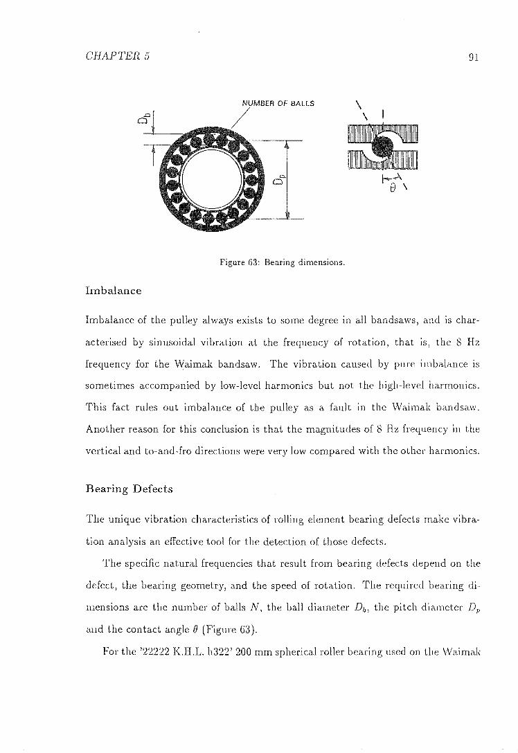
CHAPTER 5
NUMBER OF BALLS
/
o
Figure 63: Bearing dimensions.
Imbalance
\ \
91
Imbalance of the pulley always exists to some degree in all bandsaws, and is char-
acterised by sinusoidal vibration at the frequency of rotation, that is, the 8 Hz
frequency for the Waimak bandsaw. The vibration caused by pure imbalance is
sometimes accompanied by low-level harmonics but not the high-level harmonics.
This fact rules out imbalance of the pulley as a fault in the Waimak bandsaw.
Another reason for this conclusion is that the magnitudes of 8 Hz frequency in the
vertical and to-and-fro directions were very low compared with the other harmonics.
Bearing Defects
The unique vibration characteristics of rolling element bearing defects make vibra-
tion analysis an effective tool for the detection of those defects.
The specific natural frequencies that result from bearing defects depend on the
defect, the bearing geometry, and the speed of rotation. The required bearing di-
mensions are the number of balls N, the ball diameter Db, the pitch diameter Dp
and the contact angle e (Figure 63).
For the '22222 K.H.L. h322' 200 mm spherical roller bearing used on the Waimak
CHAPTER 5 92
bandsaw, there were 19 rollers around the circumference of the bearing, the diameter
of the rollers was 22 mm, the pitch diameter was 150 mm and the contact angle could
assumed to be 0 degrees.
The bearing characteristic frequencies were:
The outer ball frequency io) which is the frequency caused by a defect on
the outer race of the bearing
N (~) (I 2 27f . (35)
where n is the rotational velocity in rad/s.
• The inner ball pass frequency ii, which was the frequency caused by a defect
on the inner race of the bearing
N (~) (1 + Db coso) 2 27f Dp
(36)
• The ball spin frequency ib, which was the frequency caused by a defect on one
of the balls or rollers
(37)
• The fundamental train frequency it, which occurs at a frequency lower than
the rotation speed, and is usually caused by a severely worn cage
n ( Db ) it = - 1 - -. cos 0 471' Dp
(38)
For the Waimak bandsaw, io was 64.8 Hz, ii was 87.2 Hz, ib was 26.7 Hz and
it was 3.4 Hz.
These frequencies did not appear in the spectra, hence bearing defects were not
considered to be at fault in the Waimak bandsaw.

CHAPTER 5 93
Frequency I Hz)
Time (s)
Figure 64: Frequency spectrum of a truncated sine wave.
Misalignmen t
Misalignment takes two basic forms, preload from a bent shaft or improperly seated
bearing, and offset of the shaft centre lines of machines in the same train.
Vibration due to misalignment is usually characterised by a component at twice
the running speed and a high level of axial vibrations. spectra did not have a
high 16 Hz component, and the levels of vibration in the axial direction (side-to-side
motion) were similar to the other directions, therefore, misalignment could safely be
dismissed as a fault of the Waimak bandsaw.
Mechanical Looseness
Mechanical looseness, generally referred to as nonlinearity, almost always results
in a large number of harmonics in the vibration spectrum. The mechanism for
producing harmonics is the truncation of the response caused by looseness.
Fourier transformation of a truncated sine wave is shown in Figure 64.
Mechanical looseness appeared to be the most practical explanation for the band
saw harmonics. The slackness between the column slides and the main column, the

CHAPTER 5 94
joints between the top bearing housings and the column slides, and the contacts
between the top saw guide and the column slides are the prime suspects of the
mechanical looseness on the Waimak bandsaw. However, more experimental work
is needed to verify this point, and to suggest possible solutions to the troublesome
vibration of the bandsaw.

Chap
T ALANA
VERSE
OF A
AW LADE
6.1 roduction
Excessive structural vibrations have detrimental effects on the bandsaw as a whole,
however) the most significant impact of the vibrations IS on the cutting process.
The result of vibrations is poor cutting accuracy, of raw material, and a
decrease the production rate. The main offender is the of the bandsaw that
has immediate contact with the timber, the cutting span of the saw blade. This,
rightly enough, had been the only area of research on bandsaw vibrations for the
last twenty-five years, but until now it had not been very well understood and as
pointed out by Ulsoy and Mote in 1982 [87J that' the performance criterion) 1'elating
95

CHAPTER 6 96
band design, probably rep1'esented though the spect'rum, to the band perfoTTnance as a
wtting tool remains unresolved'. One main reason for this is because the mechanism
of cutting wood has not been thoroughly examined. Given the present technology,
the wood cutting mechanism could be investigated in much more detail. A suggested
method of analysis would be to model the tooth of the saw blade and the work piece
independently, by using the FEM, then to analyse the case when the two models
were moved into each other. This method has been mentioned by Gronlund in 1988
[26] but it was pointed out that work with this nwdel is at present far from complete.
Until the wood cutting mechanism is well understood, then and only then, the
design of a bandsaw blade as a cutting tool can be studied. The wood cutting mech-
is, therefore, a very important research area, unfortunately, it was realised
quite late, hence out of the scope for this thesis. Instead, the effects of cutting
on the stability of bandsaw blade was studied with fictitious cutting forces as in
Section 9.6.
The cutting span of the saw blade has been modelled as a moving thin beam and
as a moving plate. The two most popular techniques, used by saw blade designers to
calculate the natural frequencies of the blade, are the flexible band approximation
[52,53] and the FEM [6J. The flexible band approximation can be used for hand
calculations but only for simply-supported beams. The FEM can handle more com
plicated boundary conditions but a computer is needed for the calculations. This
chapter presents another method of analysis, the dynamic stiffness method. The
advantages of this method over the F\EM had been discussed in Chapter 4.

CHAPTER 6 97
6.2 Dynamic Stiffness Method Applied to Mov-
ing Beams
Because the main objective of this chapter is to illustrate an alternative method of
solution for the moving beam, the derivation of the problem is given in Appendix B.
A full derivation of the moving plate problem will be presented in the following
chapters and is analogous to the moving beam problem.
The equation of motion that described the transverse vibration of a moving thin
beam under transport speed 1 dependent tension is
and the boundary conditions are
v=o
av = 0 ax
EJ3v ( 2) av av or EI ax3 + (1-7]) pAc - Ro ax + pAc at = 0
or E1a2v = 0 ax 2
(39)
(40)
(41)
where v, x, t, E, I, p, A are the usual symbols for beam transverse vibration, c is
the transport speed of the beam and 7] is a constant denoting the type of straining
device.
The reasons for the terms containing c will be discussed in Chapter 8, and for
the term containing 7] is in Chapter 9.
Now, assume a separable solution of the form
v (x, t) = II (x) eiwt (42)
and substitute into Equation (39) to give
d4 11 2 . dll ( 2) d2 V EI--pAwV+2pAc(l,w)-+ (l-7])pAc -Ro -d 2 =0
dx4 dx x ( 43)
1 Axial speed of a moving beam

CHAPTER 6 98
The solution of this fourth order differential equation is
(44)
substitute this into Equation (43) to give
Elo:.'l - pAw2 - 2pAcwa ((1 'T/) pAc2
- Ro) a 2 = 0 (45)
This characteristic equation is a fourth order polynomial in a. In the case of a
stationary beam, an expression for a can be written down explicitly, however, for
the moving beam, because of the mixed derivative term in the equation of motion,
the solutions for a are very complicated (though not impossible). An easy way to
overcome this problem is to find the four values of a by using a numerical root
finding algorithm. These four values can then be used in the formation of the
dynamic stiffness matrix.
There are many robust algorithm for finding roots of polynomials. Laguerre's
method was recommended as the most straight forward and robust technique [63],
and a subroutine was also available, which could be incorporated easily into the
computer program for calculating the natural frequencies and mode shapes of the
moving beams.
The usual procedure for obtaining the dynamic stiffness matrix can now be
carried out numerically.
The complete solution is
v (46)
Referring again to Figure 18 for the positive sign convention adopted, the bound
ary conditions are

CHAPTER 6 99
p} eiwt EliJ3v ((1-11) pAc2 ) av av ax3 Ro ax + at
N2e iwt E1a2v ax2
P2Ciwt a3v 2 ) av av ax3 - ((1 11) pAc - Ro ax pAc-
at
Substitute for v from Equation (42) and Equation (46) to give
{F} ([D]l + [D]2 + [D]3) {B} ( 47)
where
p}
{F} P2
Nl
N2
Bl
{B} = B3
B4
-i (0't}3 3 . ( )3 "1 -i(0'2) -z 0'3 -i (0'4)'
i (0'1)3 eiCY1L i (0'2)3 eicxzL 3 . L 3 . L
[D]1 = EI i (0'3) C1CX3 i(0'4) C1CY4
( O'd2 (0'2 )2 ( 0'3)2 ( 0'4)2
- (0't)2 ciCY1L - (0'2)2 - (0'3)2 - (0'4? ciCX4L
Z0'1 20'2 20'3 20'4
[D]2 ((1-11)pAc2 Ro) -iO'} eiCY1L -i0'2Cicx2L -i0'3Cicx3L -i0'4Cicx4L
0 a a 0
0 a 0 0

CHAPTER 6 100
The unknown coefficients B; can be expressed, in terms of the maximum end
deflections and slopes, as
{V} [C]{B} (48)
where
or
{B} = [Cr1 {V} (49)
The stiffness matrix for a moving beam [](lm can now be found by substituting
Equation (49) into Equation (47) to give
(50)
therefore
(51)
The numerical values for this stiffness matrix can be calculated easily in a com
puter program, which can then be assembled into a global stiffness matrix using

CHAPTER 6 101
exactly the same procedure as for the stationary beam problem discussed in Chap
ter 4. The natural frequencies are found when the determinant of the global stiffness
matrix is equal to zero.
This method is the exact method hence each span of the moving beam can be
represented by one single element. It can analyse problems with any combination of
free, simply-supported, clamped and sliding end conditions. The free end condition
has not been discussed in previous publications because it was not considered as
a practical boundary condition for the bandsaw problem, ho\,vever, there are appli
cations in other fields of moving material, such as a cantilevered pipe conducting
fluid.
6.3 s of oundary Conditions on a
s Moving Beam
The bandsaw blade has been assumed to have simply-supported boundary condi
tions. Anderson (1974) [6] looked at the effects of clamped ends on the moving beam
problem and concluded that the support conditions do not have a great influence
on the first natural frequency. However, the blade dimensions chosen in Anderson's
paper were different from the dimensions of the saw blade used on the vVaimak
bandsaw. This section, therefore, attempts to compare the natural frequencies of
simply-supported end conditions and those of clamped-clamped end conditions for
the Waimak bandsaw blade. Blades with similar dimensions to those of the vVaimak
saw blade were used by Kirbach and Bonac (1978) [37,38J to investigate the effects
of tensions and axial speeds on the blades. These results were used to compare with
the results obtained by the dynamic stiffness method.
The common parameters in this study were the modulus E, the density

CHAPTER 6 102
Table 1: First two natural frequencies of a stationary blade with simply-supported and
clamped-clamped end conditions.
Length (m) S-S Beam (Hz) C- C Beam (Hz)
0.30 125.2 159.7 288.0 360.8
0.51 7l.0 I
81.6 150.3 172.5
0.83 43.1 46.8 88.2 95.8
1.00 35.7 38.2 72.5
p and the strain parameter r,. E can be assumed to be 200 X 109 N /m2• The density is
the usual 7800kg/m3, however, because the width of the blade is the width excluding
the teeth, the density was taken as 8200kg/m3 to take into account the weight of
the teeth [38]. The straining device for the Waimak bandsaw was the counterweight
mechanism, therefore, "7 = 1. The length L, the axial speed c and the initial tension
Ro were chosen as the variables for this study.
6.3.1 Varying Length
The cutting span of the blade does not have a single set length because the upper
guide is always adjusted for different log size. This means that the cutting span can
a range of frequencies depending on the position of the upper guide.
Table 1 lists the first two natural frequencies of a simply-supported beam (S-S)
and a clamped-clamped beam (C-C) for various lengths. The width of the beam
was 0.22 m and the thickness was 0.00165 m.
These results show that the first two natural frequencies of a S beam are
always smaller than those of a C-C beam, and the shorter the length, the larger
the differences in the natural frequencies. At a typical length of about 0.5 m, the
difference in the first natural frequency is about 10 Hz, or a 14% discrepancy, which

CHAPTER 6 103
Table 2: First two natural frequencies of a blade with different tensions.
I Tension (N) I S-S B~am (Hz) I C-C Beam (Hz) I Exp. Results (Hz) I
17,169. 39.6 42.4 37.2 80 .. 5 86.1
20,20l. 42.9 4.5.7 42.2 87.0 92.6
26,833. 49.4 52.2 47.8 99.8 105.4
is quite significant.
6.3.2 Varying Tension
Kirbach and Bonae (1978) [37] measured the first transverse natural frequency for
a blade with 0.237 m width, 0.0016 m in thickness and a fixed span length of
0.943 ill, at three different tensions. Table 2 shows their experimental results and
the calculated results for S-S and C-C beams.
These results also show that the frequencies for a simply-supported beam are
closer to the actual frequencies than those for the clamped-clamped beam. The
differences in the frequencies of the two types of beam are almost unchanged for
the range of tensions under investigation. It seems that the end conditions for the
cutting span of the blade are best approximated by the simply-supported boundary
conditions. Kirbach and Bonac (1978) [38] suggested that the span length of the
blade was by the distance between the outer edges of the guides instead of the
distance between the inner edges of the guides because of the curvature of the blade
as illustrate in Figure 65, therefore the measured frequencies were slightly lower
than the calculated frequencies. Although, this hypothesis seems to agree with their
experimental results, in practice the sharp edges of the would be worn off
very quickly, hence reducing the effective span length from the length between the
outer of the guides to the length between the inner edges of the guides.

CHAPTER 6 104
Outer Edge
65: Effective span length in a pressure guide system.

CHAPTER 6 105
92.0 25 43.7 43.9 46.1
87.4 88.8 93.4 50 39.3 39.6 41.6
80.9 85.2 75 ~~4.3 34.7 36.5
G8.7 71.5 75.3
6.3.3 Varying Axial Speed
Table 3 shows the natural frequencies of a S-S beam and a C-C beam for different
transport speeds. dimensions of the blade were 0.235 m in width, 0.0014 m in
thickness and 0.948 m in length, the tension was chosen to be 20,069 N.
The flexible band solution given by Mote (1965) [52] was of the form
f ( )
1/2 ( ) ( ) -l/Z n Ro pAcz pAcz - l-(l-ry)~ l+ry~
2L pA Ro Ro (52)
where f was the natural frequency in Hz, n was the mode of vibration. This so-
lution was a lower bound approximation, hence the results were slightly less than
those obtained by the dynamic stiffness method. As the axial increased the
difference between the natural frequencies of the S-S beam and those of the C-C
beam decreased.
Table 4 shows the frequencies of the vVaimak bandsaw blade with an axial speed
of 38 m/s. At a span length of 1.0 m, the difference between the first natural
frequencies is only about 4.4%, but up to 28.7% difference for a span length of
0.3 m.

CHAPTER 6 106
.-------~~~~----~=-~~~~----~~ transport speed .
0.51 63.9 73.8 141.1 162.9
1.00 31.6 33.0 65.4 70.3
6.3 Conclusion
For a typicaI bandsaw blade configurations the boundary conditions can alter the
calculated natural frequencies considerably. The simply-supported boundary condi-
tions appear to give closer results to the measured data than those obtained with
the clamped-clamped conditions.
The simply-supported boundary conditions should be used for the bandsaw blade
however, for cases where the end conditions are known to be more closely
related to the clamped conditions then the dynamic stiffness method should be used
to obtain more accurate solutions.
6.4 Multiple pan Beams
The cutting span of a bandsaw blade has been assumed to be a simply-supported
beam, however, it should be considered to be a three-span beam with the two end
supports being the points where the blade ceases contact with the two pulleys, and
the two intermediate supports being the two guides. For a three-span beam with no
tension, the lnodes of vibration are coupled, however, for a beam under high tension
the coupling effects may be negligible. This section investigates these coupling effects
on the Waimak bandsaw blade, that is, a blade with 0.22 m wide and 0.00165 m
thid\.

CHAPTER 6 107
6.4.1 Three Equal Span Lengths
The total length of the beam was taken to be 2.286 m, that IS, 0.762 m for each
equal span length.
The first four natural frequencies of the stationary three span beam with no
tension were 6.4 Hz, 8.2 Hz, 11.9 Hz, 25.5 Hz, and their mode shapes are shown in
Figure 66. These results showed that the first natural frequency was the expected
first natural frequency of a single span beam because the mode shape for each span
was the same as the first mode shape of a single beam. There were also two other
frequencies close to this first natural frequency, which were present because of the
coupling effects of the three span beam. The fourth frequency was the expected
second natural frequency of a single span.
For 15000 N tension the first four natural frequencies became 47.0 Hz, 48.1 Hz,
50.3 Hz and 96.6 Hz. Again there were three close natural frequencies, relating
to the first natural frequency of a single span beam. The tension caused the first
three natural frequencies to be closer to each other compared to those of a beam
without tension. This was because the tension became the major restoring force in
the vibration instead of the bending stiffness, therefore if the tension was assumed
to be infinitely large then there would be three identical natural frequencies which
would be equal to the first natural frequency of a single span beam, that is, the
tension uncoupled the modes of vibration of the three span beam.
For a single span beam with 0.762 m in length and axially moving at a speed
of 38 m/ s, the first two natural frequencies were 41.8 Hz and 88.2 Hz. For the
three span beam moving at the same speed, the first four natural frequencies were
41.9 Hz, 42.9Hz, 44.9 Hz and 88.2 Hz. This means that a single span beam can
be used to approximate the frequencies of the three span beam, however, there are
two other frequencies slightly higher than the first frequency due to the coupling

CHAPTER 6 108
.. ,
_',L-______ ~ ________ ~~_L ____ ~ ________ ~ _______ ,~., -0.:; UL-------~------------------------------------"
_I \L-______ ~~------~--------~--------~------~,~.,
Figure 66: First four modes of a three span beam with no tension.

CHAPTER 6 109
effects of the three span beam) in fact every frequency of the single span beam will
be accompanied by two coupling frequencies.
604.2 Long Centre S
For the bandsaw blade case, the lower guide is fixed in one position, therefore the
span length between the bottom pulley and the lower guide always remains the same
(0.786 m). The upper guide is moved to adjust for the size of the timber being cut,
this means that the span length of the centre span and the upper span are never the
same. This section considered the case when the centre span length was 1 m, and
the upper span was therefore 0.5 m long.
With no tension, the four natural frequencies were 5.1 Hz, 8.3 Hz) 15.9 Hz
and 21.2 Hz. Figure 67 shows the mode shapes corresponding to four natural
frequencies.
The first two natural frequencies of a simply-supported beam were:
§ 3.7 Hz and 14.8 Hz, for 1.0 m in length.
" 6.0 Hz and 23.9 Hz, for 0.786 m in length .
• 14.8 Hz and 59.1 Hz, for 0.5 m in length.
Comparing the results for the three span beam with the results for the three
individual beams revealed that:
ill The 1 Hz of the three span beam corresponded to the first natural frequency,
3.7 Hz) of the centre span. The coupling effects of the other two spans caused
an increase in the frequency of the three span beam .
• The 8.3 Hz corresponded to the 6.0 Hz of the 0.786 m span.

CHAPTER 6 llO
."1--_----,--,,,-, _____ ,-:,' __ ~ __ __'. ,
., ., , ",.~-----'--,'-, ---,-----:, ,-----::-----'
Figure 67: First four natural modes of a three span beam with 0.786 m, 1.0 m, 0.5 m span lengths
under no tension .
• The 15.9 Hz corresponded to the 14.8 Hz of both the first natural frequency
of the 0.5 m span and the second natural frequency of the 1.0 m centre span .
• The 21.2 Hz of the three span beam seemed to be closest to the 23.9 Hz second
natural frequency of the 0.786 m span.
The first four natural frequencies of the three span beam under 15000 N tension
were 36.9 Hz, 46.6 Hz, 73.2 Hz and 76.8 Hz. The first two natural frequencies of
each individual span were:
35.7 Hz and 72.5 Hz, for 1.0 m in length.

CHAPTER 6
~ 45.6 Hz and 93.4 Hz, for 0.786 m in length.
~ 72.5 Hz and 153.8 Hz, for 0.5 m in length.
111
The mode shapes of the three span beam are in Figure 68. These mode shapes
together wi th the frequencies of the single span beams indicate that the 36.9 Hz was
associated with the first mode of the centre span, the 46.6 Hz with the first mode of
the 0.786 m span) the 73.2 Hz with the first mode of the 0.5 m span and the 76.8 Hz
with the second mode of the centre span. This also confirms that the 21.2 Hz of the
untensioned three beam was related to the 14.8 Hz second natural frequency
of the centre span instead of the 23.9 Hz second mode of the 0.786 m span.
These results showed that the coupling effects always raise the natural frequen
cies of each beam member) and the tension on the beam reduces the coupling effects.
Therefore the natural frequencies of a high tension three span beam could be ap
proximated by obtaining the natural frequencies of each span independently which
would be the lower bounds of the actual natural frequencies. There might be more
than one actual natural frequencies associated with each approximated frequency.
At 38 m/s axial velocity, the first four natural frequencies of the tensioned three
span became 32.2 Hz, 41.4 Hz, 66.0 Hz and 70.7 Again these frequencies
could be related to the frequencies of each span.
of each individual span were:
• 31.6 Hz and 65.4 Hz, for 1.0 m in length .
• 40.5 Hz and 85.2 Hz, for 0.786 m in length.
65.4 Hz and 144.8 Hz, for 0.5 m in length.
first two natural frequencies

CHAPTER 6 112
TH·.l ... ~" • It'hUil''! .. ,!levi) ,. - 16 ~ Ml hi..rv....,4 • 1.,. •• 10" .. l':.~~" .... 1:, 1 ".
.. -,
->
-.. -« -.. " . •. > i.> • ..
-.
-..
... "'. L ___ ._.,-----.---:. ,:------:------:
Figure 68: First four natural modes of a three span beam with 0.786 m, 1.0 m, 0.5 m span lengths
under 15000 n tension.

CHAPTER 6 113
6.4.3 Short Centre Span
The characteristics of the coupling effects found in the previous sections were also
present in this 0.786 m-0.5 m-1.0 m three span beam.
With no tension, the first four natural frequencies were 4.8 Hz, 7.6 Hz, 15.7 Hz
and 22.0 Hz, and the mode shapes are shown in Figure 69. The first three frequencies
were slightly less than those of the 0.786 m-1.0 m-0.5 m beam, but the fourth one
was higher.
With 15000 N tension, the natural frequencies were 36.3 Hz, 46.5 Hz, 73.0 Hz
and 78.3 Hz. Again these were very similar to those of the previous long centre span
beam.
At 38 mls axial velocity, the frequencies were 32.2 Hz, 41.4 Hz, 66.0 Hz and
70.7 Hz. They were almost the same as those obtained for the 0.786 m-1.0 m-0.5 m
beam.
6.4.4 Conclusion
The results showed that each natural frequency of a three span beam under high
tension is always associated with a principal span, therefore, it is reasonable to use
a single span beam for approximating this frequency. The coupling effects increase
very slightly the natural frequencies of the single span beam.
6.5 Boundary Excitation of Moving Beams
The dynamic stiffness matrix provides a connection between the generalised forces
and the generalised displacements, therefore, a harmonic end force excitation can
be analysed by setting up the dynamic stiffness matrix, rearranging it and solving
for the instantaneous displacements of the system under investigation.

CHAPTER 6 114
,.,
,.,
Figure 69; First four natural modes of a three span beam with 0.786 o1. 0.5 111, 1.0 01 span lengths under no tension.

CHAPTER 6 115
Initially, it was thought that for a moving beam, the excitation at one end of the
beam could produce different results from the excitation at the other end, because
the beam was moving away from one end and toward the other. An analysis on
this hypothesis showed that the resonance condition for the moving beam problem
was the same as the resonance condition on a stationary beam, that is, a large
amplitude of vibration occurs when the frequency of the excitation is equal to a
natural frequency of the system, regardless the position of the excitation.
Strictly speaking, a moving beam does not have natural frequencies in the clas
sical sense, because there is no single frequency with in phase oscillation. However,
there are excitation frequencies which would cause large vibrations from small exci
tation levels. These frequencies have been referred to in the literature as the natural
frequencies of the moving beam. Similarly, the modes of oscilation related to these
so called natural frequencies have been called the mode shapes of the moving beam.
The first mode of oscillation for a simply-supported moving beam is illustrated in
Figure 70. This mode shape had been animated on a computer screen, which ap
peared as a wave moving in the opposite direction to the travelling direction of the
beam.
The experimental results on the bandsaw structure under idling condition (Sec
tion 5.7) showed that the bandsaw structure possessed a large number of frequencies
in the frequency spectrum, that is) 8 Hz and its harmonics. This means that the
blade is likely to be excited by the structure at or near a resonance frequency.
Other effects such as damping would prevent amplitude of oscillation of
the blade, however) even a small vibration amplitude can result in poor cutting ac
curacy. An improvement to the cutting performance could be made by eliminating
the harmonics of the rotating speed of the pulley.

CHAPTER 6 116
• I ~ J)' •
:r·························n ........ n ••• ~ y " I Il.l ~.) II. 4 g.~ \1-6 11.1 .... 1 .. 11
;En~ Ii lid IL.: ... J g.,o u..~ 11_& ILl iI... ".Ii I
Figure 70: First mode shape of a moving beam.

e
A CEDUR
C A ALYS
R AR PLAT
1.1 duction
The study of plate vibrations can be found in many vibration text books, notable
were work by Leissa (1969) [45,46] which considered the exact solutions for
rectangular plates with various boundary conditions. The use of the exact classical
method however, restricted to only simple problems, and since modern problems
are becoming more complicated, other means of approximating their solutions must
be employed.
A moving wide bandsaw blade, under various stress conditions can be modelled
as a moving plate under inplane stresses with two opposite simply-supported
or clamped and the other two edges free. This is a relatively problem,
and an approximate method must be used to solve it. Only Ulsoy and Mote (1980,
117

CHAPTER 7 118
1982) [86,87] studied the vibration of a moving plate using the classical Ritz and the
finite element Ritz methods. All other works on the bandsaw blade had modelled
the blade as (1, moving thin which would have been reasonable if the blade
were a narrow bandsaw blade or a wide blade with no stress variations across the
width. Modern bandsaw blades are often prestressed by rolling, and/or fitted with
back-crown, which produces stress variation across the width of the blade, therefore,
only the theory of a moving plate can be used to model the wide bandsaw blade
accurately.
Future developments on bandsaws will be directed toward automatic control
of the cutting process, which would require a much better understanding of the
dynamic stability of the blade under various excitations, such as external excitations
due to cutting forces, parametric excitations due to stress fiuctuations. Therefore,
a more general and systematic solution method is required to tackle the complex
problems with relative ease.
The aim of this chapter is to introduce a procedure for solving a general plate
problem. This procedure is designed to make use of the micro-computer in reducing
the hand calculations and if possible some of the algebraic manipulations. It will
be extended in following chapters to handle the more complicated problems
associated with the bandsaw blade.
7. Formulation - Hamilton's
The conventional method of fonnulating the equation of motion of a system is based
on the Newton's law of motion (Newtonian method). A method of formu
lation uses Hamilton's principle, which is perhaps the most advanced variational
principle of mechanics. One remarkable advantage of this formulation is that it

CHAPTER 7 119
is invariant with respect to the coordinate systel11~ used. It is, therefore, used ex-
tensively in both infinitesimal and finite theories of dynamic elasticity. Hamilton's
principle was chosen for the fornmlation of the plate problems in this thesis.
7.2.1 Hamilton's Principle
References to Hamilton's principle are in [49, page 42], [42, page 233], [98]. Briefiy,
the mathematical statement of Hamilton's principle is
(53)
where T is the kinetic energy and HI is the virtual work of the noninertial forces.
Or in words:
The actual path renders the value of the integral in Equation (53) mini-
mum with respect to all possible neighbouring paths that the system may
be imagined to take between two instants tl and t 2 ) provided the initial
and final configurations of the system are prescribed.
The virtual work done, llV, consists of conservative and nonconservative work
done.
(54)
and
(55)
where U is the potential energy
Therefore Equation (53) can be rewritten as
(56)
CHAPTER 7 120
In the case in which the forces are conservative
lt2
tl (8T - 8 U) dt = 0 (57)
After the kinetic energy T, the potential energy U, and the non-conservative work
done Mfne have been determined, the use of Hamilton's principle leads to a scalar
integral. The method of the calculus of variations can then be used to evaluate the
integral to provide the equations of motions and all necessary boundary conditions
of the system under investigation.
The equation of motion and boundary conditions of a stationary plate will be
derived as an example to illustrate the use of Hamilton's principle. Other factors
such as tension, travelling speed, cutting forces will be considered in the following
chapters.
7.2.2 Kinetic and Potential Energy of a Plate
The kinetic energy T of a stationary rectangular plate is
1 {b {' (8W) 2
T = "2 Jo Jo ph 8t dx dy (58)
where b is the width of the plate, I is the length, h is the thickness, p is the density,
'W is the transverse displacement and hence ~~ is the transverse velocity.
The potential energy of the plate caused by bending, Ub, is
1 1b l' { (82w 8
2w) 2 [( 82w ) 2 8
2w 82W] } Ub =- D -+- +2(1-v) -- --- dxdy
2 0 0 8x2 8y2 8x8y 8x2 8y2
(59)
where D is the flexural stiffness, D = 12~~3lJ2)' v is the Poisson's ratio and E is the
Young's modulus.
If there are other potential energies present in the plate, such as energies from
inplane stresses, then they must be added to the energy expression.
CHAPTER 7 121
7.2.3 Calculus of Variat
The Hamilton's principle, Equation (57), can now be used to give the equation of
motion and the boundary conditions of the plate. Assuming that the operator 5
and a/at, as well as 5 and a/ax, are commutative, and that the integrations with
respect to t and x are interchangeable, the method of integration by parts can be
used to expand Equation (57).
The kinetic energy term can be considered by adding a small variation to Equa-
tion (58)
T 5T
Discarding second order term and simplifying gives
5T = rb r1 ph ow a dx dy
Jo Jo at at (60)
Therefore
(61)
because 5w vanishes at t tl and t - t 2.
(62)

CHAPTER 7 122
Integrating Equation (62) by parts and rearranging gives
(2 8U elt = (t2 D { (b (I [84w + 2 8
4w + 8
4w]8W dx dy
Jtl Jtl Jo Jo 8x4 8x28y2 8y4
+ -+v- - -+ 8w ib
[(82W 82w) 8(8W)11 (8
3w 8
3w) II
o 8x2 8y2 8x x=o 8x3 8x8y2 x=o
+ (1- v) 82w 8(8w) II 1 dy
8x8y 8y x=o
+ (I [(82W + V 8
2w) 8 (8w) b _ (_8
3w + 8
3w) 8w b
Jo 8y2 8x2 8y y=o 8y3 8x28y y=o
+ (1- v) ::;y a~:):J dX} dl (63)
Adopting the sign convention as in Figure 71, the edge bending moments and
shear forces can be expressed as [35]
lI;[x -D -+v-(82w 8
2w)
8x2 8y2 (64)
lI;[y -D -+v-(82w 8
2w)
8y2 8x2 (65)
82w (66) lI;[xy D(l-v)-
8x8y
Qx -D -+ (83w 8
3w)
8x3 8x8y2 (67)
Qy -D -+ (83w 8
2w)
8y3 8x28y (68)
Equation (61) and Equation (63) can be substituted into Equation (57), and
simplified by using the edge bending moments and shear forces equations above to
glve
o (69)

CHAPTER 7 123
Q.
y/ /1 (j- Q )(
0M~y My
t 0)'
Figure 71: Coordinate directions and sign convenlion.
where
This equation contains both the equation of motion of the plate and all the
necessary boundary conditions on the edges x = 0, x = I, y - 0 and y b.
7.2.4 Equation of Motion and Boundary Conditions
equation of motion is obtained by simply equating the expression inside the
double integral of Equation (69) to zero
(70)
Note that /5w = 0 is the trivial solution, which states that if there is no displacement,
there is no vibration.
expression inside the integral f dy denotes the boundary conditions along
the x = 0 and x = I.

CHAPTER 7 124
They are
or (71)
which means that either the bending moment /Y[x or the slope in the x-direction
must be zero along the two edges.
Mxy = 0 or (72)
which means that either the twisting moment /vlxy or the slope in the y-direction
must be zero along the two edges.
Qx = 0 or fiw 0 (73)
which means that either the shear force Qx or displacement must be zero along
the two edges.
Similar boundary conditions along the edges y o and y = b can be written
down from the expression inside the integral J dx.
These boundary conditions make physical sense, and are the same as those ob-
tained from Newtonian method.
7.3 Exact olutions for Plates wit imple Boun-
dary ouditions
Although the exact solutions are restricted to simple boundary conditions, it is
important to understand those solutions which fully describe the behaviour of the
plate. Approximate solutions for more complicated problems can then be explained
and understood by relating to this information.
The types of boundary conditions are abbreviated as SS for simply-supported, C
for clamped and F for for example, SS-C-SS-F means a rectangular plate with

CHAPTER 7 125
edge x = 0 simply-supported, y 0 clamped, x = Z simply-supported, and y b
free.
The equation of motion (Equation (70)) has solutions of the form
(74)
where Wn are functions of x and y only and Wn is the nth angular natural frequency.
Substituting this expression into Equation (70) gives
where
phw;
D 12 (1 - v 2
) pw; Eh2
(75)
Let two opposite edges of the plate parallel to the y-axis be simply-supported,
then the shape function lif1n takes the form
(P7rX) Wn = f (y) sin -Z- (76)
which when substituting into Equation (75) yields
(77)
that ).2 > (Pf r the solution has the form
fp (y) Clp sin {3y + C2p cos {3y + C3p sinh,y + C4p cosh,y (78)
where
{32 ).2 - (P; r ,2 ).2 + (P;) 2

CHAPTER 7 126
7.3.1 S SS-SS-SS lates
\"'hen the two edges y = 0 and y b are simply-supported, the boundary conditions
on those edges are w = 0 and My O. Because 10 = 0 along those = 0,
and therefore = O. Hence
10 0
f)210 o (79)
on y 0 and y b.
Equation (74), Equation (76) and Equation (7S) can be substituted into the
boundary conditions to give the frequency equation as
sin{3b = 0 (SO)
therefore
where q is the mode number in the v-direction. equation can be rearranged to
w ((P7r)2 (q7r)2) ( Eh2 )1/2 1 + b 12p (1 v2 )
(S2)
The vibratory forms are
lXT A' p7rX . q7ry 'V n = SIn -1- sm b (S3)
The first four modeshapes of a plate are plotted Figure 72.
7.3.2 SS-F-S Rectangular Plates
When the two edges y 0 and y = b are free, the boundary conditions on those
edges are i'vfy = 0, .Mxy 0 and Qy = O. However, three boundary conditions on

CHAPTER 7 127
First mode Second mode
Third mode Fourth mode
72: First four modes of a SS-SS-SS-SS rectangular plate.

CHAPTER 7 128
one edge are too many to be accommo dated in the thin plate small deflection theory
(though they can be accommodated in the large deflection theory).
It has been shown that 1I1xy can be thought of as vertical forces - &~~Y can
be combined with Qy giving one condition (Qy &~;y) = O. This term is sometimes
referred to as the Kirchoff's shear force. Substituting the relevant expressions for
My, Mxy and Qy in terms of w gives
o
o (84)
on y 0 and y = b.
The frequency equation for the SS-F-SS-F plate can be found by substituting
Equation (78) into the boundary conditions above. After some lengthy, though not
difficult, algebraic manipulation, the frequency equation is given as
2 (1 (PIP4 P2P3). b' b cosfJbcosh,b) + -- - smfJ smh, = 0 P2P3 P1P4
(85)
where
(P1r)2 Pl _fJ2 - v -Z
There is no closed form solutions for this frequency equation, and a numerical
roots finding method is needed to obtain the required natural frequencies. The
vibratory shapes of the plate are given by Equation (78), and the coefficients can
be found arbitrarily by substituting the frequency of interest into the four boundary
conditions.
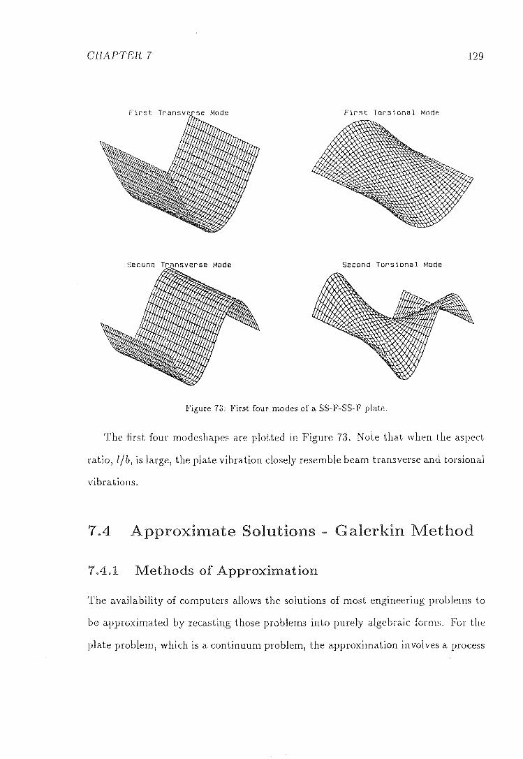
CHAPTER 7 129
First Torsional Mode
Second Torsional Mode
Figure 73: First four modes of a SS-F-SS-F plate,
The first four modesha.pes are plotted in Figure 73. No'te that when the aspect
ratio, lib, is large, the plate vibration closely resemble beam transverse and torsional
vibrations.
7. Approximate Solutions - Galerkin Method
7.4.1 Methods of Approximation
The availability of computers allows the solutions of most engineering problems to
be approximated by recasting those problems into purely algebraic forms. For the
plate problem, which is a continuum problem, the approximation involves a process
CHAPTER 7 130
called discretisation. In such a discretisation, the infinite set of numbers represent
ing the unknown functions is replaced by a finite number of unknown parameters.
Some of the common discretisation methods used in plate theory are the finite differ
ence method, the Rayleigh method, the Rayleigh-Ritz method, the weighted residual
method, and the finite element method.
The finite difference method involves a direct discretisation of the differential
equation by setting up discrete grid points on the space variable and using Taylor's
series expansion to set up the algebraic problems, [99]. It is probably the simplest
method, however, its convergence is poor compared with other methods, because a
large number of grid points is always necessary to achieve the required accuracy.
The Rayleigh's method is an energy method, where a rough estimation of the
mode shape is used to calculate the maximum kinetic and potential energies. Equat
ing the two energies will yield an approximate natural frequency. This method is an
upper bound approximation, and the closer the chosen shape function to the true
mode shape, the better the result. The Rayleigh-Ritz method extends the Rayleigh's
method from one single mode shape to a series of shape functions so that the accu
racy of the method can be improved by increasing the number of shape functions in
the series. This method is quite popular and can be used successfully in most plate
problems [97].
The weighted residual method (WRM) is another very popular method. It uses
the trial functions as in the Rayleigh-Ritz method, but instead of substituting into
the energy terms, the weighted residual method attempts to approximate the govern
ing equation itself. It is more systematic and more general than the other methods
[99]. The finite difference method and the Rayleigh-Ritz method can be thought of
as subsets of the weighted residual method. There are many methods of weighted

CHAPTER 7 131
residual, of which, the Galerkin method is the most widely used because of its com
putational efficiency.
Instead of using continuous trial functions, as in the weighted residual methods,
the finite element method (FEM) proposes to use piecewise trial functions, which
enables the method to approximate many problems involving complicated shape
functions. This makes the FEM one of the most powerful tools in the field of
computational mechanics today. Because of its generality, the FEM does suffer
inefficiency and the accuracy of the method is difficult to predict.
The weighted residual method is ideal as the method of solution for the band saw
blade problem, because if the teeth are neglected, the boundaries are simple, and
there exist continuous trial functions for those boundary conditions. It is also well
suited for other applications such as stability under parametric excitation [78] and
stability under non-conservative forces [43,44].
The Galerkin method was chosen as a discretisation method for all the plate
problems dealt with in the remaining chapters. The rest of this chapter is devoted
to setting up a general procedure to discretise the equation of motion using the
Galerkin method with the help of a computer.
1.4.2 Galerkin Method
Generally speaking, the weighted residual method is used to approximate a set of
governing differential equations defined in some region 51
£.(w)=o (86)
and a set of boundary conditions defined on the boundary r
B (w) = 0 (87)
where £. and B are differential operators and w is a variable.

CHAPTER 7 132
If w is a function of x only, then it can be approximated by
111
w(;r)~w(x) (88) m=l
or if w is a function of x and y (two dimensional) as in the plate problern
M N
w ,y) (89) m=l n=l
where am, amn are the coefficients and 'if;ml 'if;mn are the t1'ial functions. For brevity,
assume that the chosen trial functions satisfy all the boundary conditions in Equa
tion (87). Such trial functions are usually referred to as compa1'ison functions,
whereas admissible functions refer to functions which satisfy only the geomet1'ic
boundary conditions (or sometimes referred to as the essential boundary conditions)
and not the natur'al boundary conditions.
If w is substituted into the differential equation, a nonzero residual, R, is obtained
from
£ (w) = R (90)
By introducing a set of weighting functions, {Nr ; l' = 1,2, ... }, R can be forced
to be zero over the domain, D
10 NrRdD = 10 Nr£(~v) dD = 0
Equation (91) is the basis for the weighted residual method.
(91)
There are a number of methods available for choosing the weighting functions,
such as the point collocation method, the subdomai'n collocation method, the least
squa1'es method, and the Gale1'kin method. The Galerkin method is by far the most
popular '!\IRM, which makes the obvious choice of taking the trial functions them-
as the weighting functions, that is
l' = 1,2, ... ,Iy! (92)

CHAPTER 7 133
or as in the two dimensional case
{ r: 1,2, ... ,At
s-l,2, ... ,N (93)
This leads to a set of M X N equations to be solved
M N
I: I: J 1 £ (w) 1/Jrs dO = 0 r=1 s=1 !1
(94)
When substitute 1/J into the above equation, and integrate, a set of algebraic
equations is found and can numerically be solved for the required solutions. In
the case of dynamic analyses, eigenvalue problems are created, for example, in the
vibration analysis the natural frequencies are the eigenvalues and the modeshapes are
the eigenvectors, and in the buckling analysis the eigenvalues represent the buckling
loads and the eigenvectors represent the buckling configurations.
7.5 Plate Solutions Using Galerkin Method
The simple case of SS-SS-SS-SS plate will be used as an example to illustrate the
steps involved in obtaining the natural frequencies, and mode shapes using the
Galerkin method.
7.5.1 Discretisation of the Plate Equation
By substituting the solutions w = vV(x, y)eiwt into the equation of motion (70), the
governing differential equation, £ (w) can be written as
(95 )
vV( x, y) can be approximated by a series of trial functions
M N
W ~ vV = I: I: amn 1/Jmn (x) y) (96) m=1 n=1

CHAPTER 7 134
The above expression can be substituted into the Galerkin equation (94) to give
o (97)
which can then be integrated and rearranged to give
(98)
It is probably worth noting at this that m, n are subscripts associated with
the trial functions, and r, s are associated with the weighting functions. Also Tn
and r are related to the x variable while nand s are related to the y variable. The
following analyses will adopt the convention that nand s will vary fastest, therefore,
the state variable vector {X} is
{X} - (99)
So an element of [Kj, referred to as K rsmn , is at row ((r l)N + s), and column
((m - l)N + n).
The elements of [K] and []\If] are given by
(100)
and
(101 )

CHAPTER 7 135
At this stage, the boundary conditions not entered the analysis. The bound-
ary conditions are considered when selecting the appropriate trial functions, which
would satisfy all the boundary conditions explicitly, that is, the trial functions cho-
sen are comparison functions. This is a restriction on the choice of trial functions
and in Section 7.7, the extended Galerkin method is used to overcome this restriction,
so that only admissible functions are required.
7.5.2 SS-SS-SS-SS Plates
For a SS-SS-SS-SS plate, the trial functions are chosen to be
./, . (m7rx) . (n7rY\ 'f/rnn = SIn -1- sm -b-) (102)
These functions satisfy all the boundary conditions for plate (Equa-
tion (79)). In fact, these functions are the exact shape functions for the plate (Equa
tion (83)), therefore, the solutions obtained by the Galer kin method are expected
to be those obtained by the exact method.
The trial functions can be differentiated to give
[(m7r)4 (rn7r)2 (n7r)2 (n7r)4]. (m7r) " (n7r) ~ + 2 - - + - sm ~ sm -lib b' 1 b
(103)
Each term in the matrices [1\1] and [I<] can be found individually by evaluating
the don ble integrals
1\1rsrnn
I{rsmn
r = 1TI and s=n
{ ~ [( ~~ r + (nb~ rr ' 0,
(104) or si'n
r = 1TI and s = n
r i' Tn or s i' n
(105)

CHAPTER 7 136
These equations show that both [K] and [1\1] are diagonal matrices. This is a
typical characteristic of the Galerkin method because of the orthogonality property
of the chosen trial functions.
The eigenvalues and eigenvectors of Equation (98) can now be found. In this
case, the eigenvalues a.re simply
(106)
or rearrange using A defined from Equation (75) to give
w = ((7)' + ("n') (~r (107)
which is the same as the exact solution in Equation (82).
Functions for the SS-F Plate
vibratory forms of the SS-F-SS-F plate is not as simple as those of the SS-SS-
SS-SS plate, due to the two natural boundary conditions along the two free edges.
exact shapes can be deterrnined by the solutions presented in Sec-
tion 7.3. The shape functions are separable in x and y coordinates,
HI (x, y) - X (x) y (y) (108)
and because the two edges on x = 0, x = I a.re simply-supported, the shape functions
in the x direction take the form
m7rx) X (x) = L sin I
m=l
(109)
The shape functions in the y direction are quite complicated because they have
to satisfy the natural boundary conditions (Equation (84)).
Although, it is possible to use those functions in the Galerkin approximation,
they are very cumbersome and inefficient. A more feasible set of functions to use is

CHAPTER 7 137
the set of eigenfunctions for a free-free beam [97,8]. These eigenfunctions are only
admissible functions and do not satisfy all the natural boundary conditions.
One other type of functions which has been successfully applied to plate vibration
problems is the orthogonal polynomials [9,19]. These polynomials offer an attractive
alternative to the classical beam-functions. They were claimed to be more accurate,
although there are no other advantages, such as satisfying the natural boundary
conditions.
Because there was no comparIson between the use of the orthogonal polyno-
mials and the beam-functions as trial functions for the plate problems, the beam
eigenfunctions were chosen. This choice also made more physical sense than the
polynomials type. The orthogonal polynomials could be used at a later stage to
compare with the results presented in this thesis.
Young [97] suggested the functions for a free-free beam as
1
Yz J3 (1- 2:) EnY EnY (. EnY . EnY) cosh -b- + cos -b- - An smh -b- + sm -b- ,n = 3,4, ...
w here En and An can be found from
cos En cosh En - 1 = 0
A = cosh En - COS En
n sinh En - sin En
(110)
(111)
(112)
The equation for En must be solved numerically by searching for the roots. Yl
and Yz are the rigid body translation and rotation of the free-free beam respectively.
They are included to obtain a complete orthogonal set.
Bassily and Dickinson [8] suggested that the above shape functions were not
'strictly mathematically justifiable and can lead to inaccurate or el1'oneOllS results'.
They proposed the use of degenerated (or relaxed) beam functions.

CHAPTER 7 138
The above beam functions for a free-free beam can be rewritten into a simpler
form by separating the symmetrical modes from the anti-symmetrical modes as
followed
where
1
cosh Ene + An cos Ene, for n = 3,5, ...
(symmetrical mode)
(antisymmetrical mode)
1- 2y b
and En and An can be determined from
tan En + ( -1 r H En 0, n 3,4, ...
(113)
(114)
(115)
(116)
The concept of the degenerated beam functions involved the relaxation of the
unnecessary beam end conditions imposed through the particular choice of An and
En in accordance with the above relations. Instead, An and/or En can be floated,
hence can be found by the approximation itself.
This idea would improve the accuracy of the higher modes but not as much for
the first few modes. Only the first few modes of the plate vibration were of interest,
therefore, the usual beam functions were used. The degenerated beam functions
could be looked at in future studies, to see if there is actually improvement on the
efficiency of the analysis and the accuracy of the results.
first four values of en and An are listed in Table 5.

CHAPTER 7
3 2.02875 78381 1043 4 4.49340 94579 0906 5 4.91318 04394 3488 6 7.72525 18369 3771
-4.16583 350794104 -45.80106 48489 7487 69.42692 66490 5937
1141.85924 27107 2200
139
7.7 Extended Galerkin Method for SS-F-SS-F
Plates
It is impractical to find a set of trial functions which satisfy all the natural boundary
conditions imposed by the two free edges. If possible, admissible functions would
provide a simpler option to solve the SS-F-SS-F plate problem.
It is noted that the Rayleigh-Ritz method requires only admissible functions
as its trial functions, and the reason for this is because the boundary conditions
are already included in the potential energy expression of the plate. This becomes
obvious if referring back to the formulation of the plate equation using Hamilton's
principle, where both the equation of motion and the boundary conditions were
produced from the kinetic and potential energies. This means that the Rayleigh
Ritz method approximates both the equation of motion and the boundary conditions
simultaneously, whereas the Galerkin method described previously considered only
the equation of motion. One way to extend the Galerkin method is to include the
boundary conditions in the approximation, then admissible functions will be allowed
as the trial functions of the Galerkin method. This method is sometimes referred to
as the Extended Galerkin method [99, page 57].

CHAPTER 7 140
7.7.1 Extended Weighted Residual Method
This method is an extension to the weighted residual method described in Sec
tion 7.4.2, which relaxes the requirement that the trial functions must satisfy the
boundary conditions B (w) = O.
If a set of trial functions chosen to approximate the problem does not satisfy
some or all of the natural boundary conditions, then the residual in the domain, Rn
given by
Rn = t (w), mn (117)
is supplemented by a boundary residual Rr
Rr = B (w), on r (118)
The weighted sum of the residuals on both the domain and the boundary is
(119)
hence
(120)
where, in general, the weighting functions N r and Nr can be chosen independently.
The first term of the above equation can often be rearranged to
(121)
where C, 'D and £ are linear differential operators involving an order of differentiation
lower than that of the original operator t. This rearrangement is often referred to
as the weak form of the weighted residual method.
When Equation (121) is substituted into Equation (120), it may be possible to
simplify or even eliminate the two terms in the boundary integral Ir by choosing
suitable boundary weighting functions Nr •

CHAPTER 7 141
When the weighting functions N r and Nr are chosen to be the trial functions
or their derivatives, then the extended weighted residual method, described here, is
called the extended Galerkin method.
7.2 Weak Form of the Equation
first term in the weighted residual approximation of the plate equation
can be integrated by parts to reduce the order of differentiation
where \7 2 is the Laplace operator
When the boundary geometry of the plate is more complicated than the rectan-
gular case, such as the circular plate problem, then the dive1'gence them'em should
be used instead of the integration by parts [49, page 179].
7.7.3 S s lates
The boundary conditions on the two simply-support edges, x o and x = I, are
already satisfied by the trial functions, sin ( mfx ) , hence there is no need to approx
imate them in the analysis.
The bounda.ry conditions on the two free edges are, however, required in the
approximation, because the trial functions do not satisfy them explicitly.

CHAPTER 7 142
Applying the extended Galerkin method to the plate equation of motion (Equa
tion (75)), and the boundary conditions (Equation (84)) gives
= 0 (123)
The weak form, Equation (122), can be then substituted into the first term of
Equation (123), hence
Recalled that Nrs and N: s are independent weighting functions, and by letting
Equation (124) can be simplified to
(125)
Equation (125) shows that when the trial functions do not satisfy all the natural
boundary conditions, the Galerkin equation contains extra terms in the boundary
integral.

CHAPTER 7 143
708 A Computer-Oriented Procedure
When the plate problem becomes more complicated, the work involved in obtaining
the solutions also becomes more tedious. Because the main purpose of discretis
ing the problem is to allow a computer to carry out this time-consuming task of
arithmetic, a systematic procedure is developed in this section to utilize fully the
computer capability for solving these problems.
From the previous section, the two steps that involved a lot of computations were
the double integrations of each term in the [111] and [f{] matrices and the eigen value
solver.
Both of these mentioned steps can be carried out numerically by using a com
puter. At present, the use of personal computers (PC) are very popular because of
their powerful capabilities and low prices. Developing the solver on a PC was more
convenient and will, perhaps, be more useful to others than if done on a main frame
computer.
7.8.1 Eigenvalue Solver - PC-MATLAB
PC-1I1ATLAB is an interactive computer program that serves as a convenient labora
tory for computations involving matrices. It provides easy access to matrix software
developed by the LINPACf{ and EISPACf{ projects [20,74]. MATLAB was initially
written in Fortran and designed to run on mainframe computers. PC-MATLAB is
the second generation of MATLAB for the IBM-PC. It had been completely rewrit
ten in the C language and included many new features which made it a flexible
and powerful scientific spreadsheet for many types of numeric calculations, not just
matrix computations.

CHAPTER 7 144
A multi-purpose eigenvalue solver is a very complex piece of software [63,74]. PC
MATLAB comes fully equipped with a set of powerful routines for solving eigenvalue
problems, the EISPACK routines. These routines, together with the flexible inter
active environment, and the way in which YlATLAB handles mat.rices, make it the
obvious choice for solving the eigenvalue problems presented in this Its only
shortcoming would be the allowable 100 X laO maximum size for a matrix. So far,
the matrices involved in this thesis had been smaller than laO x lOa.
7.8.2 Numerical Integration
The integration step could also be handled by YlATLAB using its own interpreted
language, which would give a much more compact coding than that written by
Fortran to perform the same task. However, the integration procedure required for
the Galerkin plate problem is very complicated, a separate computer program would
be more feasible. values calculated could then be imported into MATLAB for
the second phase of the analysis, the search for eigen values.
The method of numerical integration will be dealt with in Section 7.9.
7.8.3 Computer Language - The C Language
There are many indications that C can be used as a very powerful computer lan
guage for scientific purposes, it was therefore chosen as the computer language for
developing the program to perform the integration. A of C's better features,
compared with the more conventional languages, such as Fortran, include
• More powerful control structures, such as while, swdch.
More versatile data types such as pointers) structures, unwns. These data
types enable the true dynamic memory allocation of variables, which means

CHAPTER 7 145
that there is no longer a need to set aside a large block of memory while a
particular application may require only a small portion of this. This feature is
very useful when programming on a PC where memory is more limited than
on a mainframe computer.
iii Much better file and I/O handling.
iii The powerful concept of libraries. This enables a function which has more
than one application to be saved in a library and therefore can be accessed at
a later date by other programs.
iii Compatibility. C is believed to be the most compatible language of all.
One of the best reference available for numerical analyses in C is the "Numerical
Recipes in C" [64].
7.8.4 The Procedure
The procedure adopted is as follows:
1. The problem is formulated using Hamilton's principle to provide the equation
of motion and all the boundary conditions. The equation of motion of the plate
is a partial differential equation in time and two dimensional space domains.
£(w(x,y,t)) = 0
where £ is a partial differential operator.
2. Assume a separable solution of time and space
w(x,y,t) = H!(x,y)T(t)
where T( t) is a function of the time variable, and H!( x, y) is a function of the
space variables.

CHAPTER 7 146
3. Choose trial functions to approximate the solutions H!(x,y) of the governing
equation, by trying to find functions which satisfy all the geometric bound
ary conditions and as many of the natural boundary conditions as possible.
Differentiations of the trial functions with respect to 1: and y will also be re
quired, depending on the governing equation. These functions are placed in
the program once for each different plate geometry. Changes in the natural
boundary conditions are taken care of by the extended Ga.lerkin formulation,
and not the trial functions themselves.
4. Substitute the governing differential equation into the Galerkin equation. For
problems where the trial functions do not satisfy all the natural boundary con
ditions, the extended Galerkin method is used to approximate the governing
equations and the natural boundary conditions simultaneously.
This step reduces the governing equation to a set of ordinary differential equa
tions, or in the case of linear vibration analysis a set of a.lgebraic equations,
which can be expressed in matrix form.
5. Simplify the problem by integrating by parts and choosing appropriate weight
ing functions to eliminate as many terms in the boundary integration as pos
sible.
6. Rearrange the Galerkin equation so that most of the parameters, such as
the flexural rigidity, the density, the thickness, the transport speed, and the
magnitude of tension, are not included in the program. These parameters can
be defined interactively in MATLAB. The dimensions land b of the plate,
and the profiles of the stresses (as in Chapter 9) are however, needed in the
program.

CHAPTER 7 147
7. Write computer subroutines which use the trial functions and any other differ~
en tiations of the trial functions to calculate the terms required for the in tegra~
tions. Cycling over l', s, m and n, and using the numerical integration routine
to compute each element of the matrices given in the matrix equation. The
numerical values of those matrices can be saved in a MATLAB~format data
file.
8. Enter the MATLAB environment, read the data file, define all the parameters
required for the
eigenvalues and
set up the matrix equation and finally solve for the
\far'TArQ of the equation.
7.9 Integration - Gaussian Q ....... """'."-'L.L
ture
There are many numerical integration schemes available, of which, the most popular
scheme is Gaussian quadrature, therefore it was chosen to perform the integration
required in this thesis.
A one dimensional Gaussian quadrature rule is given by
that is, I is approximated by evaluating <P (e) at each of several locations ei, multi
plying <p (ei) by an appropriate weight Ni , then adding them together. The
points ei, sometimes called the Gauss points, and the
z 1, 2, ... , n are determined by the Gauss method to provide the
Numerical values of the Gauss points and weights are given in [14,
be calculated using the computer program given in [64, page 136].
Ni for
accuracy.
120], or can

CHAPTER 7 148
Similarly, for a two dimensional case
Note that the Gauss points and the weights are given for 1 ~ ~ ~ 1 and
-1 ~ 17 ~ 1 ; for the plate problems in this thesis, the integrations over the area of
the plate are for 0 ~ x ~ I and 0 ~ y ~ b, therefore transformations of coordinates
are required before they may be integrated, thus
(128)
In general, a polynomial of degree 211. - 1 is integrated exactly by 11. Gauss
points. For all the calculations in this thesis, eight Gauss points were chosen for
each direction, that is, a fifteenth degree polynomial could be integrated exactly.
er 8
MOVING ES
8.1 Introduct·
A wide bandsaw blade, when stationary, can be analysed usmg the usual plate
model, however, under idling or cutting conditions, it must be represented by a
moving plate.
The moving plate model belongs to a class of problems referred to as the axially
moving material problems. The first investigation into these problems was the study
on an axially moving in 1897 [73]. It was not until 1965 when the first research
on the bandsaw vibration was published by Mote [52] which was on the transverse
vibration of a moving beam. Since then, research on bandsaw blades has escalated
and diverged into many different areas, such as the torsional vibration of a moving
beam [5,75], the parametric excitation of a moving beam under fluctuating tension
[58]. The first investigation of a moving plate problem was published in 1980 [86,87],
which pointed out that the moving plate theory \vas necessary to model a wide
bandsaw blade.
Recent research had been directed toward more complicated subjects, such as,
149

CHAPTER 8 150
the coupling between the transverse and torsional vibration of a movmg beam
[75,95], the coupling between the cutting and non-cutting span of the bandsaw
blade [94,88,891, the stability of a moving beam under a periodic edge loading [95].
These studies revealed many interesting phenomena, however they did not consider
the moving plate case.
Chapter 7 had discussed a method of analysing plate problems, and had
considered the vibration analysis of stationary plates. This chapter presents a step
which extends the theory of stationary plates to cover the moving plate problem .
8.2 . Ion
The Hamilton's principle discussed in Section 7.2 was used to formulate the equation
of motion and the boundary conditions of a moving plate.
An actual saw blade is always subjected to a large tensile force which increases
the stiffness of the blade and therefore increases the potential energy of the plate.
For brevity, the inclusion of this extra potential energy due to the tensile force is
deferred until the next chapter. The potential energy of a moving plate is, therefore,
the same as that of a stationary plate, and Equation (59) and (63) are still valid for
this case.
kinetic energy of a moving plate is obtained by finding the velocity of the
wi th to a stationary spatial coordinates system, (x, y, z). The material
coordinates system, (Xl, yl, Zl), is moving with a velocity c along the x direction with
to the stationa.ry coordinates (see Figure 74).
Assume arbitrarily that a.t time t = 0 the two coordinates are coincided,

CHAPTER 8 151
x ( t
Figure 74: Spatial and material coordinates.
then at time t
X Xl + ct
y yl (129)
z Zl
The time dependent lateral displacement of the plate referenced to the material
coordinates is WI(XI,yl,t) or referenced to the spatial coordinates is w(x,y,t), They
are, in fact, same displacement but referred to by a different coordinates system,
hence
I (I I t) - (I W X ,y 1 = W X + yl, t) (130)
The lateral velocity of a plate with respect to the moving frame of reference is
simply ) and from the definition of partial differentiation, this velocity can be
expressed as
awl I' [WI (Xl, yl, t + 6.t) = 1m
at 6t~O 6.t Wi (Xl, yl, t) 1
(131 )
Substituting the expression in Equation (130) into the above equation to give
awl lim
w (Xl, yl, t) at 6t~O
lim w +c6.t,y,t+
1 (132)
6t~O 6.t
This IS actually the defmition of a total derivative with 6.x c6.t and

CHAPTER 8
6y 0, hence
ow' Dw (x, y, t) Dt
ow ow -+c--at ox
The absolute velocity of a vibrating moving plate is
V [c2 + (aa~'rr [c
2
+ (~~ + c~:rr hence the kinetic energy is by
T 1'].' P2h
[C2 + (~~ + C ~: r] dx dy
152
(133)
(134)
(135)
When c = 0, Equation (135) becomes Equation (58) the kinetic energy of a
stationary plate.
Applying the calculus of variations as illustrated in Section 7.2 to the kinetic
energy Equation (135) gives
OZw OZw) o 0 +c2
-0 Ow dx dy x t x 2
b ow ow ( )
I } + 10 phc ot + c ox ow x=o dy dt (136)
Substituting Equation (136) and Equation (63) into the Hamilton's equation
(Equation (57)) gives the equation of motion of an axially moving plate as
On x = 0 and x I, the boundary condi tions are
'11J 0 or ( ow phcOt
+ ow ) ox - Qx = 0
ow 0 A1x - 0
ox or
ow =0
oy or A1xy 0
(137)
(138)
(139)
(140)

CHAPTER 8 153
and on y = 0, y = b
w =0 or Qy = 0 (141 )
ow =0 oy
or 1I1y = 0 (142)
ow -=0 ax
or Mxy = 0 (143)
The terms c2 32
w d 2 32
w can be regarded as the centripetal term, and the 3x2 an c 3x3t
coriolis term respectively.
8.3 Approximate Solutions for a Moving SS-F-
SS-F Plate
8.3.1 Galerkin Equation
The method of solving the moving plate problem is similar to that for the stationary
plate in Section 7.7. The extra terms in the boundary conditions do not affect the
solution, because the edges along x = 0 and x = l are simply-supported, that is,
w = o. Therefore, only two extra terms in the equation of motion are to be added
to the stationary plate solution. The boundary conditions on the y = 0, y = b edges
remain the same as previously.
The trial functions are exactly the same as for those used in the stationary
plate case, because there are no changes in the boundary geometry. For the sake
of generality, instead of assuming w(x,y,t) = lV(x,y)eiwt, w(x,y,t) = W(x,y)T(t)
was used, which when substituted into the Galerkin equation will produce a set of
second-order ordinary differential equations, instead of a set of algebraic equations.

CHAPTER 8 154
Applying the weighting functions, 'ljJrs, on the two extra terms due to the trans-
port velocity, c, and combining with Equation (125) gives
Note that the third term the above equation can be simplified by using inte-
gration by parts
rb 'ljJrs avV t dy _ rb rt a'IjJrs oW dx dy io ax x=o io io ax ax
rb t a'IjJrs oW dx dy (145) io io ax ax
since 'ljJrs 0 at x = 0 and x l.
Rearranging Equation (144) into a matrix form, and separating out the parame
ters D, p, h, c from the matrices. These matrices will be evaluated by the numerical
integration routine.
ph [A] {i'} + 2phc[B] {t} + (D [CJ + phc2 [DJ) {T} = 0 (146)
where the element of [AJ, [BJ, [C] and [D] are
Drsmn
Referring to Section 7.5.1 for the meaning of the subscripts T, s, Tn, n.
CHAPTER 8 155
For vibration analyses, {T} is assumed to be
{T} {X} eAt (147)
where {X} represents .the generalised coordinates vector as in Equation (99). Sub-
stituting this into the second-order differential equation to produce a quadratic
eigenvalue problem. The complication here is the existence of a lU."",""U derivative
term in the equation of motion, which becomes a first order differential term in
the Galerkin equation. A special technique is, therefore, required for solving the
quadratic eigenvalue problem.
8.3.2 Quadratic Eigenvalue Problems
For simplicity, Equation (147) combining with Equation (146) can be rearranged to
a more general quadratic eigenvalue form
(148)
One method of obtaining the eigenvalues of the equation directly is by using an
inverse iteration method [47]. Another method available is the linearisation of the
quadratic eigenvalue problem [2,78], which is perhaps less efficient than the inverse
iteration, but much simpler in principle. The linearisation method was chosen for
solving the quadratic eigenvalue problems in this thesis.
Equation (148) can be rearranged by shifting the ).2 term to the right hand side,
and pre-multiplying the equation by [M2r1 to give
(149)
Introducing a new variable {Y} = ). {X}, and combining with Equation (149)
gIves
(150)

CHAPTER 8 156
where [0] is a zero matrix, and [I] is an identity matrix, both are the same size as
[Mol·
This augmented equation can now be solve for the eigenvalues), by the usual
eigenvalue solver such as the one provided by PC-MATLAB.
Note that the number of eigenvalues found by this method is twice the number
of the eigenvalues found for the stationary plate. This is because), contain the
eigen values of the linearisised equation, whereas, the stationary plate eigenvalues
are ),2, which are, in fact,

hapt
S R A DSAW
BL
9.1 Introduction
The bandsaw blade is subjected to large in-plane stresses for a number of reasons,
some of the reasons are intended by the designer, while some are produced from the
interactions of the saw blade with other parts of the machine during its operation.
In 1972 Pahlitzsch and Puttkammer [60] and later in 1985 Allen [3] investigated
the cause of stresses occurring in bandsaw blades. A recent improvement on the
dynamic behaviour of a saw blade was achieved by introducing a higher stress level
than that in the conventional blades. The improved bandsaw is sometimes referred
to as a high-strain bandsaw. This development has pushed stress to the limit
of the elastic strength of the material, hence reducing life expectancy of the
blade. A result of excessive stress in the saw blade is the development of cracks in
the gullets of the saw teeth.
This subject of stressing bandsaw blades is still not fully understood because
157

CHAPTER 9 158
all the work carried out so far has been from observation in production, or from
experiments or based on basic theories of strength of materials. A plane-stress finite
element analysis of the blade in the region of the tooth and the gullet would have
been quite useful, unfortunately, it was out of the scope of this thesis.
The dynamic behaviour of a stressed wide bandsaw blade is also inadequately
understood, therefore, this chapter extends the plate theory presented in the pre-
vious chapters to include the effects of in-plane stresses, and investigates various
patterns of stress occurring in bandsaw blades.
9.2 General Formulation and Method of Solu-
tions
9.2.1 Formulation
In plane-stresses of a plate consist of a direct stress in the x direction CY x, a direct
stress in the y direction CYy and a shear stress Txy. Since the thickness of a saw blade
is constant, a more convenient unit of measurement for the stresses are forces per
unit length, that is, N x = CYxh, Ny = CYyh, N xy = Txyh, where h is the thickness.
These forces per unit length raise the potential energy of the plate, therefore,
they have to be included into the potential energy of the previous plate model. The
total potential energy of the plate, U, can then be expressed as
(151 )
where Ub is the potential energy caused by bending, which was given by Equa-
tion (59), and V is the potential energy caused by the in-plane forces
b I 1 ow ow ow ow { ( )2 ( )2}
V = 10 10"2 Nx ox + 2Nxy ox oy + Ny oy dx dy (152)

CHAPTER 9 159
The variation of this term can be written down and integrated by parts using
the method described in Section 7.2 to
--N-+-N-+ N··-l t2 {ib il [0 ( ow) 0 ( ow) 0 ( ow) tj 0 0 ox x ox oy y oy ox xy oy
o ( OW) 1 ib [ow ow 1 -j- -- .\T - dx dy + N - + N - ow :::l • xy ;:) x :::l xy :::l (}y (}x 0 (}x uy
ely
+ l' [N, ~; + N., ~: 1 bw C dX} dt (153)
The equation of motion and the boundary conditions can be found by combining
Equation (153) with Equation (63) and Equation (61) for the stationary plate case
or Equation (136) for the moving plate case.
For a stationary plate, the equation of motion is
and the boundary conditions on x = 0 and x I are
flix = 0 or ow
0 (155) 0;<;
flixy = 0 or ow
0 (156) oy
or w =0 (157)
and on y = 0 and y b are
ow 0 (158) oy
flixy 0 or ow
0 (159) ox or w 0 (160)

CHAPTER 9
Similarly, for a moving plate the equation of motion is
and the boundary conditions on x 0 and x l are
or
lvlxy = 0 or
ow = 0 ox ow = 0 oy
(OW 20W
phe- + phe --at ax Ow ax Nxy ~; - Q x) = 0
or w o
and on y 0 y bare
Illy = 0 ow
0 or oy
Mxy = 0 ow
0 or ax ( ow . ow )
Ny oy + Nxy ax + Qy = 0 or 'W = 0
9.2.2 Method of Solutions
160
(162)
(163)
(164)
(165)
(166)
(167)
The trial functions for the SS-F-SS-F plate in Section 7.6 are still valid for both the
stationary and the moving plate problem in this chapter, and the Galerkin equations
can be constructed the same way as described previously.
There are four extra terms in the boundary conditions due to the in-plane
stresses, which can be simplified by combining with the terms in the equation of
motion using the weak-form of the Galerkin method discussed in Section 7.7.2 . By
this method, the terms in the equation of motion are first integrated using

CHAPTER 9 161
the method of integration by parts, then the terms in the boundary integral can
be combined or even cancelled out with the four terms in the boundary conditions.
That is
where 7f;rs is the trial functions, and the weighting functions of the Galerkin method.
Again, the boundary integral on x - 0, x 1 is equal to zero because of zero
displacement (7f;rs = 0). The boundary integral on y O,y b is of the same
form as the boundary conditions, therefore, it can be cancelled out by selecting
the appropriate weighting functions for the boundary conditions. This leads to the
general Galerkin equation for a moving plate under in-plane stresses as
o (169)
For a stationary plate, the Galerkin equation is the same as Equation (169) with
c O.

CHAPTER 9 162
Stresses due to t tatic Tension
The lateral stiffness of the saw blade is very low 1 therefore, a large tension is required
to stiffen the blade during idling and cutting conditions. The mechanism of applying
the tension, the straining device, been discussed in Chapter 2.
9.3.1 Stress Characteristics
This static tension can be to be uniformly distributed across the width of
the blade. It is velocity dependent, because an increase in the transport velocity of
the blade would cause an increase in the centripetal acceleration, which is required to
keep the band in tight contact with the pulley surface. This centripetal acceleration
is provided by the straining mechanism. For the counter weight mechanism, the
pressure between the pulley and the blade is always kept constant, the total
tension on the blade is
Ro h 2 N x -[; +p c (170)
where Ro is the static initial tension force (N). Hmvever, the unit of measurement
for N x is force per unit width (N 1m), therefore, a new variable qo was introduced to
represent the magnitude of instead of ROJ where
Ro qo=-
b
For other types of straining device, such as the air-strain mechanism, the extra
tension required to take up the centripetal effect may be less than phc2, a constant
1] was, therefore, introduced to represent this effect
(171 )
where 0 ::;: 7l 1. 7l 1 represents the counter weight mechanism, 1] = 0 represents
the rigid pulley support. For an air-stra.in mecha.nism 1] can only be ohtained from

CHAPTER 9 163
Table 6 First two natural frequencIes of a plate under vanous stress eve s.
Stress Experimental F for Frequencies for (N/mm2
) Frequencies (Hz) 2x2 Functions (Hz) 3x3 Functions (Hz)
·15.3 37.2 39.6 39.6 43.4 45.3 45.3
53.3 42.2 43.0 43.0 47.7 48.2 48.2
70.8 47.8 49.4 49.4 54.l 54.1 54.1
experimental results. Typical values of 1( are close to 1 [86].
The static tensioning of the blade does not affect Ny and Nxy , hence
The vVaimak bandsaw uses a tension level of, approximately, 15000N in force,
that is, a stress of 41 N/mm2, or a force per unit width 68000 N/m.
Kirbach and Bonae experiments [37] used stress levels 45.3, 53.3, 70.8 N /mm2
for similar blade dimensions to those of the Waimak saw blade.
9.3.2 Stationary Plates under Tension
The first two natural frequencies for a plate, 0.237 m wide, 0.0016 m thick and
0.943 m long, are presented in Table 6 together with the experimental results of
Kirbach and Bonac [37]. For brevity, the number of modes assumed for a trial
function was denoted by III X N, where J'I1 is the number of modes in the x direction
and N is the number of modes in the y direction. Therefore, a 2 x 2 trial function
would produce 4x4 matrices in the Galerkin equation and hence four eigenvalues, a
3x3 trial function would produce nine eigenvalues.
The first two natural frequencies for the plate, calculated with the 2x2 trial
function were the same as those calculated with the :3 X 3 trial function, however, the
HLF,HvL natural frequencies of the 3 x 3 function calculation would be more accurate

CHAPTER 9 164
Table 7: First two natural frequencies of the vVaimak saw blade at various lengths and t,ransport
speed.
1.0 m
25 33.8 40.8
38 31.8 39.0
50 29.6 133.0 75.7 36.9
75 98.0 53.1 1 120.0 67.0
than those obtained with the 2 X 2 function. Table 6 shows that the theoretical
results were very close to the experimental results.
T'he first natural frequencies were associated with the first transverse mode of
the plate and the second natural frequencies were associated with the first torsional
mode of the plate.
These results showed that the natural frequency of the first torsional mode was
close to the natural frequency of the first transverse mode of the bandsaw blade,
therefore, it was difficult to predict which mode of vibrations would be the principal
mode of the blade.
9.3.3 Moving Plate under Tension
Table 7 shows the calculated frequencies for the \i\laimak saw blade for three different
span lengths.
The first transverse natural frequencies were the same as those calculated from
the moving beam theory in Chapter 6. The first torsional frequencies were the second
frequencies of the plate, which also decreased as the transport speed increases. The

CHAPTER 9 165
Table 8: First two natural frequencies of a blade at various transport speeds.
Speed Experimen tal Frequencies for Frequencies for (m/s) Frequencies (Hz) 2x2 Functions (Hz) 3x3 Functions (Hz)
0 40. 45.9 45.9 49.7 49.7
25 37.5 44.2 44.2 48.2 48.2
50 34. 40.4 40.0 44.5 44.2
75 29. 36.0 35.1 40.2 39.3
effect of varying transport speed on a short blade was greater than that on a longer
blade.
The first two natural frequencies for a plate with a thickness of 0.0014 m, a width
of 0.235 m, a length of 0.948 m and subjected to a tension of 61 N /mm2 were also
calculated for various transport speeds and presented in Table 8 and Figure 75.
The calculated results were about 6 Hz higher than the experimental results of
Kirbach and Bonae [38]. This discrepancy was probably due to the difference in
actual span length of the blade and the measured length as explained in Chapter 6.
As expected, both natural frequencies decreased ~ith increasing transport speed.
Note that at high transport speed, the calculations with the 3x3 trial function
gave frequencies that were in better agreement with those found experimentally than
did those with the 2x2 function l .
As pointed out in Chapter 7, the moving beam theory was adequate for a wide
saw blade with a uniform stress distribution across the width, such as the results
presented in this section. The following sections vvill consider non-uniform stress
distribution on bandsaw blades, which obviously cannot be determined by the beam
theory.
1 Galerkin method is an upper bound method, therefore, the lower the result the more accurate it is.

CHAPTER 9
Frequency (Hz) 60.---------------------------------------------------~
50r=~------~~----__ _ 40
30
20
£:::,. lat Tr&na • .Exp.
10 -t-!zIt Tr&na .• Theo.
~ ht Tora .• Theo.
OL------------L------------~----------~------------~
o 20 40
Speed (m/s) 60
Figure 75: Natural frequency versus transport speed.
80
166
9.4 Stresses due to Wheel-tilting and Back-crow-
. nlng
Wheel-tilting and back-crowning, as described in Chapter 2, can be assumed to
induce linear stress variations across the width of the blade. The main purpose of
this is to provide a higher tension on the cutting edge than that on the back edge,
which is desirable for the stability of the blade during cutting [71]. Allen [3] stated
that another reason for back-crowning is to compensate for the temperature gradient
between the cutting edge and the back edge of the blade during cutting.
9.4.1 Stress Characteristics
To represent the linear stress variation across the blade, N x can be modify to
( 172)

CHAPTER 9 167
where d and e are parameters which characterise the distribution of Nx .
ill For a uniform tension, d 1 and e O.
ill For a triangularly distributed load, d 1 and e = -l.
ill For a pure bending, d 1 and e
Again, the other in-plane stresses are not affected by the wheel-tilting and/or
back-crowning) hence
It is very difficult to measure the amount of wheel-tilting accurately) therefore
the values of d and e cannot be given from the angle of tilt. A more accurate way
of determining d and e is to measure directly the stresses at the cutting edge and at
the back edge. This method is satisfactory for experimental studies but not feasible
in practice.
The magnitude of back-crown is indicated by the diameter D of a circular arc
along the back of the blade, or conventionally, the maximum distance 8 be-
tween a straight and the circular arc of the back edge over a specified length
L (Figure 76). A typical value for back-crown is 0.4 mm in a length of l.524 m. AI-
though, the effects of fitting back-crown to the saw blade are well understood, there
is no published theoretical study of those effects; to enable them to be accurately
predicted by theoretical calculations.
Allen [3] provided a formula for calculating the stress induced by back-crown,
which is
Eb 48Eb (fEC = ±]j = L2 (17:3)
where E is the Young's lTlOdulus and b is the width of the blade.

CHAPTER 9
D/2 I
Figure 75: Stress due to back-crown.
9.4,2 Wheel-tilting
168
Kirbach and Bonac [37J presented the first two natural frequencies of a blade at
various amounts of wheel-tilting and various tensions. The amount of tilt was given
by the stress ratio / between the back edge and the cutting edge) that is) / = 1 for
uniform stress) and / = 0 for zero stress on the back edge.
If qo in Equation (172) represents the initial static force per unit width, then the
two parameters d and e could be found by
d 2
-- e 1 +,'
2(/ -1)
1+/ (174)
Tables 9) 10) and 11 list the experimental results of Kirbach and Bonac, and
the theoretical results obtained in the present investigation at three different stress
levels. These values were also plotted in Figures 77, 78, and 79.
These results show that the theoretical calculations were closely correlated to
the experimental results found by Kirbach and Bonac. Wheel-tilting results ll1
a decrease in the first transverse natural frequency and an increase in the first
torsional frequency of a blade. While a small amount of wheel-tilting may improve
the performance of the blade, too much tilt would have a destabilising effect on the
blade because of the low first transverse natural frequency.

CHAPTER 9 169
Table g. First two natural frequencies for various stress ratios, at 45.2 N jmm 2 static stress.
Stress Ratio Experimental Theoretical
I Frequencies (Hz) Frequencies (Hz)
I l. 37.2 39.6 43.5 45.2
0.8 37.7 39.3 43.5 45.5 I
0.6 38.0 38.4 45.0 46.2
0.4 38.0 36.8 48.0 47.5
0.2 37.7 34.0 54.0 49.5
O. 37.5 29.4 60.0 52.2
Frequency (Hz) 70.-----------------------------------------------------.
60 .... . ..... +
50r--+-" ··-.... 2· .. ·~· .. ·~.".~~~;_;~~-____!J._..--J I U .... .1 " "
• .. ...... "t' .............. , ...... +, .............. , .... . 40
" ...... "' .................. t"'1 •.•• ,.'"
20
10
,..., ~
.................... :0 .................... ..
I:::: ht Traru .• El::p.
1st Ton., El::p.
-S- lilt Traru .• Thoa.
-+- lilt Torti .. Thoo.
O~---------L--------~~--------~--------~~--------~
o 0.2 0.4 0.6 O.B 1
Stress Ratio
Figure 77: Natural frequency versus stress ratio, at 45.2 Njmm2 stress level.
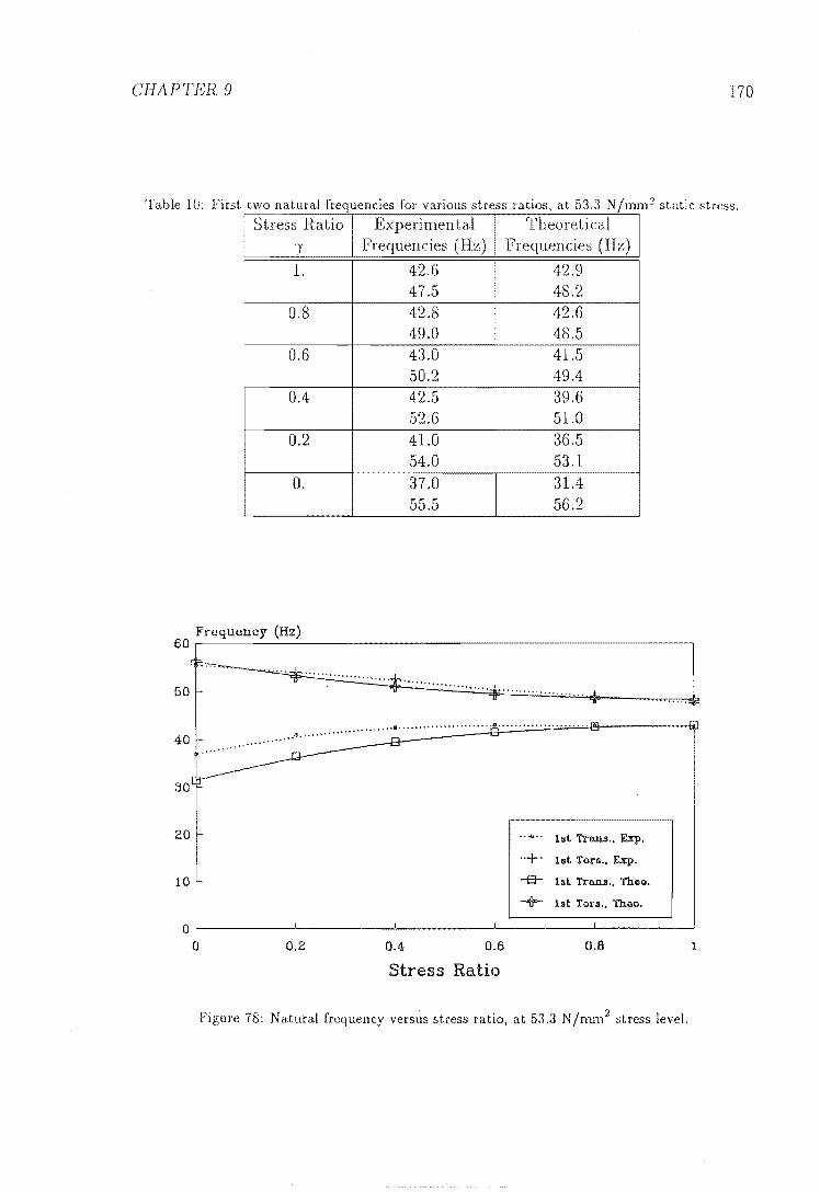
CHAPTER 9 170
Table 10: First two natural frequencies for various stress ratios, at 53.3 Njmm 2 static stress . . ~-Stress Ratio Experimen tal Theoretical ., Frequencies (Hz) Frequencies (Hz)
l. 42.6 42.9 47.5 48.2
0.8 42.8 42.6 49.0 48.5
0.6 43.0 4l.5 50.2 49.4
0.4 42.5 39.6 52.6 51.0
0.2 4l.0 36.5 54.0 53.1
O. 37.0 31.4 55.5 56.2
Frequency (Hz) 60,-----------------------------------------------------,
50 .~ ..... : .............. + ...................... ~ ..
u ............... '::}
•••.• , •.•••• eo .•. ~ •••••.•.•.• ~ ..••• r!-;, .................. . r&I.
40, ................ ~
30[~
20 1st Tr!Ul.3 .. Exp .
. +. l:!l Ton., Exp.
10 . -B-- ht Tr!Ul.3., thOll.
I
-+- ht Tors .• Theo.
0 0 0.2 OA- 0.6 0.8 1
Stress Ratio
Figure 78: Natural frequency versus stress ratio, at 53.3 Njmm2 stress level.

CHAPTER 9 171
Table 11: First two natural frequencies for various stress ratios, at 70.8 N/nun 2 static stress.
Stress Ratio Experimental Theoretical
I Frequencies (Hz) Frequencies (Hz)
l. 47.5 49.4 54.0 54.1
O.S 47.5 49.0 54.0 54.5
0.6 46.5 47.5 54.2 55.S
OA 45.0 45.1 55.0 57.7
0.2 42.5 41.3 57.0 60.3
O. 39.0 35.1 60.0 63.9
Frequency (Hz) 70r-----------------------------------------------------,
60 ....... .............. + .................... .
50
30
20
10
.....................
........... ............................................ ,
ht TrlUllil., Exp.
0+. ht Torti., Exp.
-B- hl TrtUlll., ThelD.
lilt. Tara., Thoo.
O~---------L--------~----------~--------~--------~
o 0.2 0.4 0.6
Stress Ratio
0.8
Figure 79: Natural frequency versus stress ratio, at 70.8 N/mm2 stress level.
1
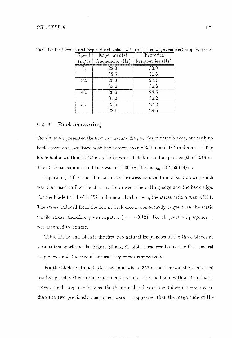
CHAPTER 9 172
Table 12: First two natural frequencies of a blade with no back-crown, at various transport speeds.
Speed Experimental Theoretical (m/s) FreqllpnC'lPs (Hz) Frequencies (Hz)
I
O. 29.0 30.0 32.5 31.6
I 32. 28.0 29.1 32.0 30.8
43. 26.0 28.5 31.0 30.2
53. 25.5 27.8 28.0 29.5
9.4.3 ack-crowning
Tanaka .aL u\.d'",,"U the first two natural frequencies of three blades, one with no
back-crown and two fitted with back-crown having 352 m and 144 m diameter. The
blade had a width of 0.127 m, a thickness of 0.0009 m and a span length of 2.16 m.
The static tension on the blade was at 1600 kg, that is, qo =123590 N 1m.
Equation (173) was used to calculate the stress induced from a back-crown, which
was then used to find the stress ratio between the cutting edge and the back edge.
For the blade fitted with 352 m diameter back-crown, the stress ratio., was 0.3111.
stress induced from the 144 m back-crown was actually larger than the static
tensile stress, therefore., was negative h = -0.12). For all practical purposes, .,
was &"lsumed to be zero.
Table 12, 13 and 14 lists the first two natural frequencies of the three blades at
various transport speeds. Figure 80 and 81 plots these results for the first natural
frequencies and the second natural frequencies respectively.
For the blades with no back-crown and with a 352 m back-crown, the theoretical
results agreed well with the experimental results. For the blade with a 144 m back-
crown, the discrepancy between the theoretical and experimental results was greater
than the two previously mentioned cases. It appeared that the magnitude of the

CHAPTER 9 173
Table 13: First two natural frequencies of a blade with 352 In hack-crowll, at various transport
speeds,
O. 27.0 25.9 34.0 35.0
32. 25.0 24.9 33.0 34.3
43. 24.0 24.2 31.0 33.7
53. 22.0 23.5 30.0 33.1
Table 14: First two natural frequencies of a blade with 144 In back-crown, at various transport
Speed Experimental Theoretical (m/s) Frequencies (Hz) Frequencies (Hz)
! O. 25.0 20.7 37.0 38.3
32. 24.0 19.5 35.0 37.6
43. 22,0 18.6 ! 34.5 37.1
53. 20.0 17.8 33.0 36.5

CHAPTER 9 174
Frequency (Hz) 35.-----------------------------------------------------.
30[p.~ .. ~ ... ~ ... ~ ... ~ .... ~ ... _: ... =~---------_ . ••••••••••••••••••••••••••••••••••••••• '""IiP~
......
20
........ . ..... ............. "'0' 25c~ .. ~ .. ~ .. ~ ... ~.~~~~: .. ~ .. ~ .. ~ .. ~ .. ·~ .. ~ .. ~ .. ~ .. ~ ... ~"~ .. ~"~ .. ~~= __ ~~~~'~ .. ~ .. ~"~·"~ .. ~"~ .. ~.D i ... ' ..... ' ......................................... ~.... ..· .. ··v
........•.. .; ••••.••.•.••••. : 15 ··G· No B.C., Exp. .. ",. :::loam B.C., Exp. .. y. 144m. B.C., Exp.
No B.C., Thllo. -7f- :::I5am B.C., Thea. 144m. B.C., Thea.
10 0 10 20 30 40 50 60
Speed (m/s)
Figure 80: First natural frequencies versus transport speed, for blades with various back-crowns.
Frequency (Hz) 40~----------------------------------------------------.
~i> ......... ................................ --r 35 .................... t' .................. ~
;;.:::::::ii..........~ 30 r-
'LJ
25 ... G· No B.C., Exp. .. ",. :::loam B.C .• Exp. . .y . 144m B.C .• Exp. -- No B.C., Thea. -7f- :::I6am H.C .. Theo. -+- 144m B.C •• Thea.
20~-------L--------L--------k--------~------~------~
o 10 20 30 40 50 60
Speed (m/s)
Figure 81: Second natural frequencies versus transport speed, for blades with various back-crowns.

CHAPTER 9 175
stress induced by the back-crown was than that calculated with Equation (173).
It was not clear whether the inaccuracy of the results was from Equation (173) or
from the measurement of the back-crown. However, in general, the assumption that
back-crowning produces linearly distributed stresses across the width of the blade
appeared to be correct, and its effects were to decrease the first transverse frequency
and to increase the torsional frequency of the blade.
To test the validity of Equation (173) for estimating the stresses induced by
back-crowns, experimental measurements of the stresses across the width of the
blades fitted with various back-crowns have to be carried out and compare with
those obtained by (173). This subject is left for future investigation.
9.5 s due to Prestressing
It was found experimentally that, by stretching the central area of a blade in re
lation to the two longitudinal edges, a saw blade with a better performance was
produced. stretching process has been referred to in the literature as tension
ing or prestressing. In this thesis, the stretching process will only be referred to as
prestressing.
is no published theoretical study to determine the optimum value
for a particular blade. The Saw Doctors performing the prestressing process can only
use experience in estimating the amount of prestress.
reasons for prestressing a bandsaw blade are
To counteract the expansion which take place during the cutting operations.
To stiffen the cutting edge so that it resists the cut.
To ensure that the saw runs in a constant position on the pulleys.

CHAPTER 9
\ \ \
B
\ I
\ / \ I \ I \ / \ ~/ \ II
\ I
\ I \ II
\ I \1
Figure 82: Bent bandsaw blade and transverse deflected shape.
9.5.1 Stress Characteristics
176
It was explained that the prestressing process improves the performance of the blade
because it sets up residual stresses in the blade. It is very difficult to measure the
residual stresses accurately, and in the past, Saw Doctors have controlled the level
of prestress by measuring the light gap [) when the blade is bent over a given radius
[25] (see Figure 82). This light gap is measured by using tension gauges, and these
are graded in numbers, for example, 26, 28, 44, the numbers being the diameter (in
feet) of a circular arc (see Figure 83).
It was found experimentally that a parabolic distribution of the residual stress

CHAPTER 9 177
N
~\l\llll'\ll\~ Figure 83: Tension gauge index number.
across the width of the blade gives better sawing accuracy than any other stress
distribution [4].
A theoretical calculation of the light gap 5, ven the radius of curvature R, the
width b, the thickness h, and the residual stress distribution O'x(y), was presented
by Foschi [25], which considered the differential equation
( 175)
This equation is closely related to that of the anticlastic curvature of nat plates.
For a parabolic residual stress
(y 1)2
O'x (y) = -O'c + 120'c b - 2 (176)
where 0' c is the magnitude of the compressive stress at the cen tre of Lhe blade. At
the edges y 0, y b, Equation (176) gives a tensile stress of O't

CHAPTER 9 178
The solution of Equation (175) can now be used to express the light-gap, 8, for
this parabolic stress as
8 h
[lie + 24Zl [a1 (1 cosh/, cos/,) - a2 sinh/,sin/,] + Z where
e=~ Rh
sinh /' cos /' - cosh /' sin /'
(sinh 2/, + sin 2/,)
sinh /' cos /' + cosh /' sin /'
( sinh 2/, + sin 2/,)
8 can also be obtained from Figure 84 for any particular e and {3.
(177)
Foschi also pointed out that a particular transverse deflected shape may not
represent a unique residual stress distribution, concluded that the light
technique cannot be considered as a reliable estimator of the residual stresses. Nev-
ertheless, this technique is, at present, the only means of non-destructive test for
measuring the prestress.
In this the prestress on the blade is assumed to produce a parabolic
residual stress distribution, and the magnitude of the stress can be approximated
from Figure 84, given the magnitude of the light gap, 8, the radius of curvature, R,
and the dimensions of the blade.

CIlAPTER 9
2.0
1.8
1.0
1.2
1.0
8/T
fl; 10 PARABOLIC STRESS OISTRIBUTION
-0,2 ih 0 (ANTlCL-ASTICI
Figure 84: Light gap for parabolic residual stresses.
179

CHAPTER 9 180
Kirbach and Bonac [37], and Tanaka et.al. [80] had shown experimentally that
the prestress on bandsaw blades results in a slight decrease of the first lateral natural
frequency and a marked increase of the first torsional natural frequency. Ulsoy and
Mote [86] had also verified these effects theoretically, by applying a parabolic in
plane stress, N x to their plate model. However, there was no discussion of the
magnitudes of the prestress used. It is very important to find out if the magnitude
of a prestress could be estimated from the tension gauge number, and whether or
not this prestress value could be used to obtain accurately the natural frequencies
of the saw blade.
The parabolic prestress could be incorporated into the plate problem presented
in this thesis by letting the in-plane stress N x be
(178)
where qs is a magnitude in force per unit width, and d, e, f are parameters which
define the stress distribution. If f = 0 this equation becomes Equation (172). For
the prestress in Equation (176), d = 2, e = -12, f = 12 and qs = h(J"c'
Other stresses such as the static tensile stress or the stresses due to wheel tilting
and/or back crowning, can be superimposed on the prestress distribution, for exam
ple, a prestressed blade, which is statically strained to qo, would have a distribution
of
The other two in-plane stresses are no longer zero and can be found by con
sidering the compatibility conditions, the equilibrium conditions and the boundary
conditions of the plate. These conditions for a two dimensional stress state are given
in text books on the theory of elasticity, such as [84, page 57-69].
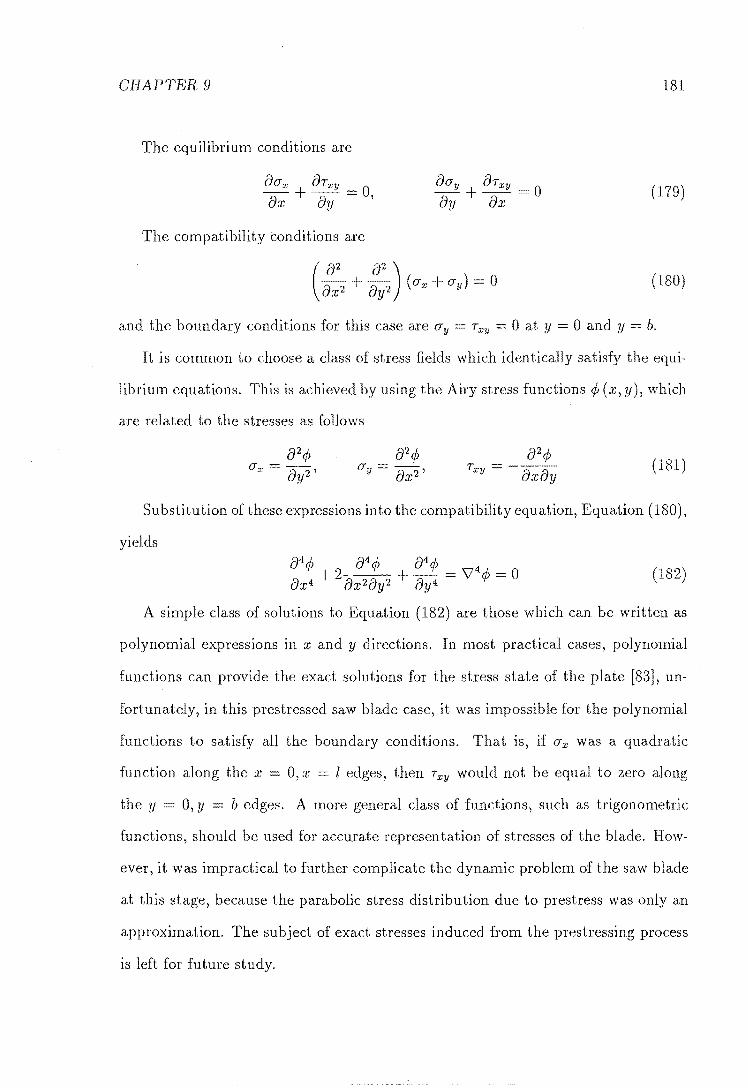
CHAPTER 9 181
The equilibrium conditions are
8er,. -'+ =0, 8x 8y
8ery 8-Txy 0 -+-8y 8x (179)
The compatibility conditions are
(180)
and the boundary conditions for this case are ery Txy = 0 at y = 0 and y = b.
It is common to choose a class of stress fields which identically satisfy the equi-
librium equations. This is achieved by using the Airy stress functions ¢> (x, y), which
are related to the stresses as follows
(181 )
Substitution of these expressions into the compatibility equation, Equation (180),
yields
84 ¢> 84 ¢> 84 ¢> 4
~ + 2 8 28 2 + 8 4 = V¢>= 0 Ox x y Y (182)
A simple class of solutions to Equation (182) are those which can be written as
polynomial expressions in x and y directions. In most practical cases, polynomial
functions can provide the exact solutions for the stress state of the plate [83], un-
fortunately, in this prestressed saw blade case, it was impossible for the polynomial
functions to satisfy all the boundary conditions. That is, if erx was a quadratic
function along the x 0, x = 1 edges, then Txy would not be equal to zero along
the y O,y b edges. A more general class of functions, such as trigonometric
functions, should be used for accurate representation of stresses of the blade. How-
ever, it was impractical to further complicate the dynamic problem of the saw blade
at this stage, because the parabolic stress distribution due to prestress was only an
approximation. The subject of exact stresses induced from the prestressing process
is left for future study.

CHAPTER 9 182
Table 15: First two natural frequencies of K&B prest.ressed blade at various static tensions.
Static Stress Experimental Theoretical (N/mm2
) Frequencies (Hz) Frequencies (Hz) .....
45.2 37.5 39.4 46.5 53.3
53.3 42.5 42.8 52.4 55.9
70.8 47.5 49.3 57.0 61.0
In this thesis, assume that O'y = Txy = 0, that is Ny 0, then obtain
the natural frequencies of the blade under quadratic stress 0' x and compare with the
experimental results published by Kirbach and Bonae [37], and Tanaka et.a1. [80l
to see if Figure 84 could be used to estimate the magnitude of the prestress.
9.5.2 Kirbaeh and Bonae Experimental Results
The experiment was carried out on a blade with a width of 0.237 m, a thickness of
a.0016m and a length of 0.943 m. The blade was prestressed to 'a profile thal is
considered in the indust1'Y as optimum for good cutting performance', unfortunately,
the magnitude of the prestress was not given in the publication. Simmonds [71, page
24] recormnended that for a blade with similar dimensions, the amount of prestress
should be about 52 gauge) that is, 2R=15.85 Ill.
From Figure 84, the magnitude of the prestress was qs 46400 N / m. The
experimental and theoretical results are listed in Table 15.
Comparison between these results and those in Table 6 showed that the pre-
stress increased the first torsional frequencies, but did not alter the first transverse
natural frequencies. The theoretical results appeared to produce the correct effects
of prestress on the blade, however, the calculated torsional frequencies were higher
than the measured frequencies. This meant that qs should be less than 46400 N/m,
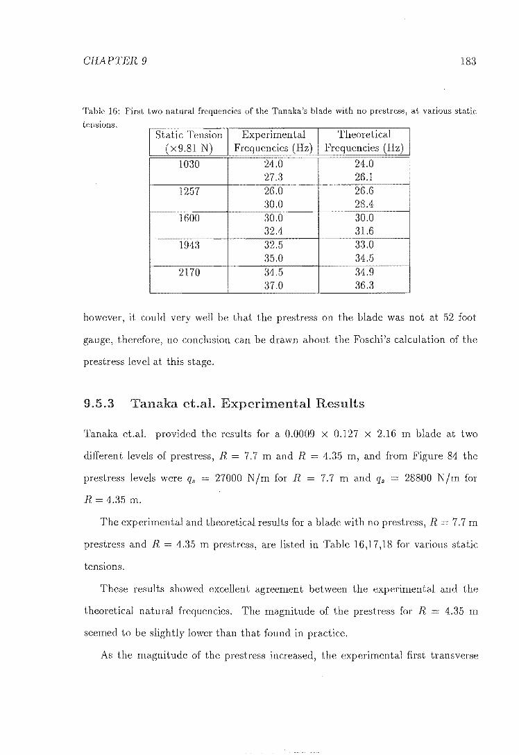
CHAPTER 9 183
Table 16: First two natural frequencies of the Tanaka's blade with no prestress, at various static
tensions. Static Tension Experimen tal Theoretical
(x9.81 N) Frequencies (Hz) Frequencies (Hz)
1030 24.0 24.0 27.3 26.1
1257 26.0 26.6 30.0 28.4
1600 30.0 30.0 32.4 31.6
1943 32.5 33.0 35.0 34.5
2170 34.5 34.9 37.0 36.3
however, it could very well be that the prestress on the blade was not at 52 foot
gauge, therefore, no conclusion can be drawn about the Foschi's calculation of the
prestress level at this stage .
9.5.3 Tanaka . al. Experimental Results
Tanaka et.aL provided the results for a 0.0009 x 0.127 x 2.16 m blade at two
different levels of prestress, R = 7.7 m and R 4.35 m, and from Figure 84 the
prestress levels were qs 27000 N 1m for R 7.7 m and qs = 28800 N/m for
R 4.35 m.
The experimental and theoretical results for a blade with no prestress, R 7.7 m
and R = 4.35 m prestress, are listed in Table 16)17,18 for various static
tensions.
These results showed excellent agreement between the experimental and the
theoretical natural frequencies. The magnitude of the prestress for R
seemed to be slightly lower than that found in practice.
4.35 m
the magnitude of the prestress increased, the experimental first transverse

CHAPTER 9 184
Table 17: First two natural frequencies of the Tanaka's blade with l' = 7.7 m prestress, at various
static tensions. Static Tension Experimental Theoretical
(x9.81 N) Frequencies (Hz) Frequencies (Hz)
1257 26.0 26.6 31.5 31.0
1600 29.5 29.9 34.5 34.0
1943 32.5 33.0 37.0 36.7
Table 18: First two natural frequencies of the Tanaka's blade with l' = 4.35 m Prestress, at various
static tensions. Static Tension Experimental Theoretical
(x9.81 N) Frequencies (Hz) Frequencies (Hz)
1030 22.5 24.0 32.5 29.1
1257 24.5 26.6 34.8 31.2
1600 27.8 29.9 37.3 34.1
1943 31.0 33.0 39.3 36.9
2170 32.5 34.9 41.7 38.8

CHAPTEn 9 185
frequencies decreased slightly, however, the theoretical frequencies remained the
same for all three cases. The first torsional frequencies increased as the magnitude
of the increased, for both the experimental and the theoretical results. The
effects of the prestress at a low static tension were greater than those at a higher
static tension.
9.5.4 Conclusion
The results in this section showed that the approximate parabolic stress distribution
in the longitudinal direction of the blade appeared to produce similar behaviour to
that of a prestressed saw blade. The magnitude of the prestress calculated from
Foschi's theory provided acceptable starting point for the cases considered in this
thesis.
However, there were still many uncertainties on the subject of prestressing, and
further experimental work needs to be carried out to answer the following questions:
• What is the actual residual stress distribution in the x direction of a prestressed
saw blade?
• Is there any residual stress in the y direction?
CiI \Vhat happens to the stress distribution when the blade is placed on the pulleys
and statically stretched?
• Is there a better residual stress profile than the parabolic type?
9.6 Stresses Induced by Cutt' Forces
This is an area of research which has been neglected in the past, perhaps because of
the difficulties in obtaining experimental results. VIsoy Mote (1980,1982) [86,87]

CHAPTER 9 186
regarded the edge forces on the plate, due to cutting, as very small and concluded
that they were not the cause of instability of the blade. \iVu (1986) [96], and \iVu and
Mote (1986) [95] have considered the effects of cutting forces on a moving beam and
shown that these cutting forces coupled the transverse vibration with the torsional
vibration. Atternpts to study the vibration of the saw blades during cutting have
been made experimentally [81,17], but there appeared to be a lack of direction and
of conclusive results. It is important that both theoretical and experimental studies
are considered together so that results from one can be verified or explained by
results from the other.
The experimental studies of the saw blade behaviour during cutting was beyond
the scope of the present investigation, but it is hoped that such studies can be made
in the future to support the theoretical results found presented here.
9.6.1 Cutting Forces
There are three main forces applied on the blade during sawing:
• Perpendicular in-plane force, Fj, on the cutting edge of the blade, due to the
work piece being fed onto the blade. The reaction forces are from the tilting
of the top wheel, and the friction between the band and the outer surface of
the pulley .
• Tangential force, Fe on the cutting edge, due to the resistance of the timber
to the cutting effects of the saw teeth.
III Perpendicular transverse force, ,may arise from the interaction between the
blade and the work piece.
Pahlitzsch and Puttkarnmer [60] concluded that the feed force, Fj, and the trans
verse force, Ft , could be neglected because they were very small compared to the

CHAPTER 9 187
Figure 85: Cutting forces on the blade.
static tension. \Vu [96,95], in his theoretical analysis, took the feed force into ac
count and showed that it coupled the transverse mode with the torsional mode due
to the reaction from the end moments, however, he did not mention the magnitude
of the feed force.
It has been observed on one bandsaw that the saw blade was pulled forward
during cutting, instead of being pushed back due to feed force. This effect can
be explained by considering the magnitude of the feed force, and the mechanism of
cutting wood.
The feed speed is dependent on the type of timber and the depth of cut. Timbers
can be graded by densi (at an approximate 15% moisture content) or more
accurately, by hardness and texture [71, page 114]. The feed rates are also divided
into basic ranges from less than 0.127 m/s to above 1 mis, with typical feed speeds
of approximately 0.5 m/s.
The blade speed is dependent on the type and size of bandsaw. For the Waimak
bandsaw, the rotating speed is about 8 Hz (50 rad/ s) and the pulley diameter is
about 1.5 m, hence the blade speed is about 38 m/s. At a very high feed speed
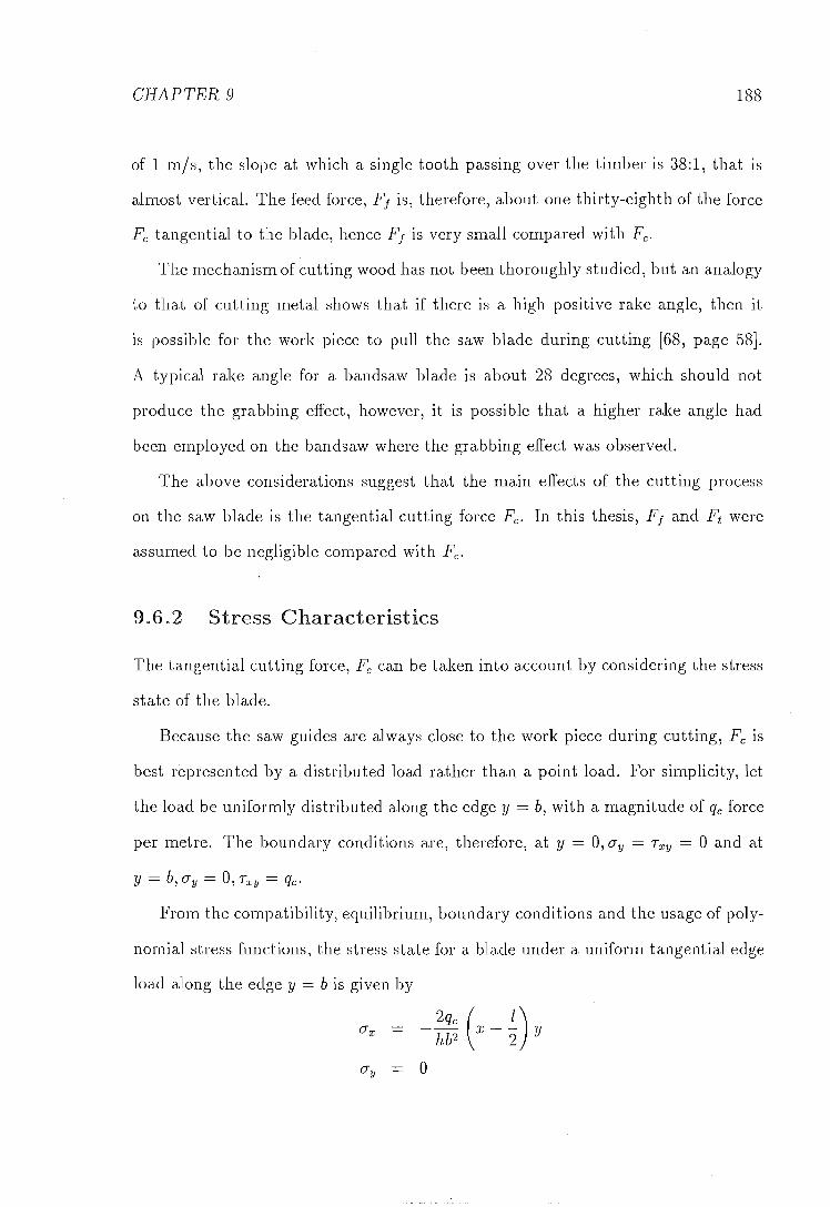
CHAPTER 9 188
of 1 mis, the slope at which a single tooth passing over the timber is 38:1, that is
almost vertical. The feed force, Fi is, therefore, about one thirty-eighth of the force
Fe tangential to the blade, hence Fi is very small compared with Fe.
The mechanism of cutting wood has not been thoroughly studied, but an analogy
to that of cutting metal shows that if there is a high positive rake angle, then it
is possible for the work piece to pull the saw blade during cutting [68, page 58].
A typical rake angle for a bandsaw blade is about 28 degrees, which should not
produce the grabbing effect, however, it is possible that a higher rake angle had
been employed on the bandsaw where the grabbing effect was observed.
The above considerations suggest that the main effects of the cutting process
on the saw blade is the tangential cutting force Fe. In this thesis, Fi and Ft were
assumed to be negligible compared with Fe.
9.6.2 Stress Characteristics
The tangential cutting force, Fe can be taken into account by considering the stress
state of the blade.
Because the saw guides are always close to the work piece during cutting, Fe is
best represented by a distributed load rather than a point load. For simplicity, let
the load be uniformly distributed along the edge y = b, with a magnitude of qc force
per metre. The boundary conditions are, therefore, at y = O,O"y = Txy = 0 and at
y = b,O"y = 0, Txy = qc.
From the compatibility, equilibrium, boundary conditions and the usage of poly-
nomial stress functions, the stress state for a blade under a uniform tangential edge
load along the edge y = b is given by
_ 2qc (x _ i) Y hb2 2
o

CHAPTER 9 189
x
y
x
Figure 86: Distribution of l7 x and Txy.
Txy =
Figure SG plots the distribution of the stresses.
A linear stress distribution along the x direction, due to static tension and back-
crown, can be superimposed on the above stress and the results can be multiplied
by h to give
( Y) I (X ) Y qo d + e- - q - 2- - 1 -b C bib
o
(183)
(184)
(185)
Note that a parabolic stress along the x direction would not satisfy the compat-
ibility conditions, therefore, this investigation only considered the tangential force
on a blade with no prestress.

CHAPTER 9 190
9.6.3 Magnitude of Cutting Forces
The magnitude of cutting forces has not been conclusively found, because, as dis
cussed in Chapter 6, the mechanism of cutting wood has not been very well under
stood.
A recent publication on this area of research was a progress report on an ongoing
project by Gronlund (1988) [26], which experimentally investigated the magnitude
of cutting forces in relation to various parameters, such as cutting speed, chip thick
ness, rake angle, clearance angle, edge sharpness, density of wood, moisture content,
hardness, and direction of the cut with respect to the fibre direction and the year
ring direction. An equation to calculate the main cutting force was given, which was
based on a non-linear regression analysis of the various measurements of the cutting
force, unfortunately there are errors in the equation which make it impossible to
use. It was mentioned that more work had to be done on improving this statistical
model.
In this investigation, the main interest was focused on the dynamic behaviour of
the bJade, therefore an approximate value of the main cutting force was sufficient.
A typical value for the tangential cutting force qc was about 1000 N/m.
9.6.4 Results for a Stationary Blade
Although, there are no practical problems associated with the stationary blade under
a tangential edge force, the following results provide a better understanding of the
effects of the tangential force on a plate, and they may also be experimentally verified
with relative ease.
A blade, with dimensions of O.22xO.00165xO.8 m and with a static tension of
15000 N, was used as a sample calculation to illustrate the effects of the tangential
cutting force.
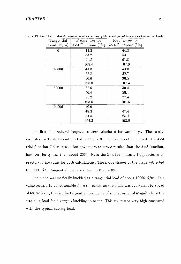
CHAPTER 9 191
Table 19: First £ t If f t f our na ura requencles 0 a s a IOnary bl db' t d t a e su Jec e t ngentialloads. o various a
Tangential for Freq . Load (Njm) 3x3 Functions (Hz) 4x4 Fu ~
0 44.8 44.8 53.2 53.1 91.8 91.8 108.4 107.9
10000 43.8 43.8 52.8 52.7 90.6 90.5 108.0 107.4
30000 32.6 30.4 50.4 50.1 81.2 77.4 105.5 104.5
40000 10.0 48.3 47.4 74.5 65.4 104.3 103.0
The first four natural frequencies were calculated for various qc. The results
are listed in Table 19 and plotted in Figure 87. The values obtained with the 4x4
trial function Galerkin solution gave more accurate results than the 3 X 3 function,
however, for qc less than about 20000 N I m the first four natural frequencies were
practically the same for both calculations. The mode shapes of the blade subjected
to 30000 Njm tangential load are shown in Figure 88.
The blade was statically buckled at a tangential load of about 40000 N 1m. This
value seemed to be reasonable since the strain on the blade was equivalent to a load
of 68182 N jm, that is, the tangential load had a of similar order of magnitude to the
straining load for divergent buckling to occur. This value was very high compared
with the typical cutting load.

CHAPTEIt 9 192
Tangential Load (N/m) (Thousands) 50.-------------------------------------------------------,
40
30
20
10
o 20 40 60 60 100 120
Frequency (Hz)
Figure 87: Natural frequency versus tangential edge load, for a stationary blade.
88: First four modes of a stationary blade subjected to. 30000 N 1m tangential load (3 x 3
trial [unction).

CHAPTER 9 193
Table 20: First four natural frequencies of a blade with 38 mls transport speed, subjected to
various tangential loads.
Tangential Frequencies for Frequencies for Load (N/m) 3x3 Functions (Hz) 4x4 Functions (Hz)
0 40.0 39.9 48.9 48.7 87.0 84.1 lO3.5 100.5
lOOOO 38.9 38.8 48.7 48.5 86.3 83.0 103.3 100.0
30000 28.0 25.7 47.1 46.6 80.6 73.2 101.5 97.3
40000 8.4 -
45.6 44.9 75.7 63.8 100.5 95.7
9.6.5 Results for a Moving Blade
The first four natural frequencies of the same blade as in the previous section, with
an axial speed of 38 m/s are given in Table 20, and plotted in Figure 89.
The overall of the transport speed was a 12% reduction in the natural
frequencies of the blade. Therefore, the buckling load was also decreased, however,
this reduction was insignificant compared with the magnitude of the buckling load.
9.6.6 Conclusion
For a typical bandsaw blade configuration, the effects of axial speed on the divergent
buckling load was minimal, therefore, a stationary blade would provide a reasonably
accurate description of the divergent buckling effect.
The magnitude of the buckling load was nlUch greater than that of a typical

CHAPTER 9 194
Tangential Loud (N/m) (Thousands) 50,-----------------------------------------------------,
40
30
20
10
O~------~--------~--~----~------~~~----_Er_----~
o 20 40 60 ~ 100 120
Frequency (Hz)
Figure 89: Natural frequency versus tangential load, for a blade with 38 m/s transport speed.
cutting load, however) this is to be expected because otherwise the present bandsaw
operation would be considered unsafe.
It seems unlikely that the magnitude of the cutting load could be as high as that
of the buckling load. However, the divergent buckling of the blade due to tangential
cutting force cannot be ruled out as a possible cause of the blade instability, because
the magnitude of the cutting load, which causes the blade to become unstable, has
not been measured.
It becomes obvious at this stage that a full experimental investigation of the
unstable behaviour of the bandsaw blade is necessary to verify many uncertainties
in this field of work.
The theory presented in this thesis provides a powerful technique for the analysis
of bandsaw blades under in-plane stresses. Until the parameters associated with the
cutting process are determined, this theory should become an important tool in the

CHAPTER 9 195
design of bandsaw blades with better performance.

S AB o A DSAW
L D UN R ARAM T c
c o
10.1 Introduction
The subject undertaken in this chapter belongs to a modern branch of the theory of
elasticity, the theory of dynamic stability of elastic systems. The counterpart of this
theory is the theory of static stability, where a static load may result in dive1:qent
buckling of the system. The dynamic stability problems involve loads which are
dependent on time (dynamic loads), snch as periodic loads. A low level dynamic
load can cause the system to have large vibrations. This phenomenon is referred
to as the parametric resonance of the system, and the dynamic load is called the
parametric excitation.
For the bandsaw blade problem, parametric excitations are present and must be
considered as possible causes of the saw blade vibration during idling and cutting
196

CHAPTER 10 197
conditions. Naguleswaran and 'Williams (1968) [58] have considered the effects of
periodic fluctuations in tension on the transverse vibration of a moving beam, due
to pulleys eccentricity, joints and flaws in the band and on the pulley surfaces.
Ariaratnam and Asokanthan (1988) [7] considered the same phenomenon but for
the torsional oscillations of a moving beam. Wu and Mote (1986) [95] addressed the
in-plane normal periodic edge load on the moving beam. However, there has not
been a published study of parametric excitations of a moving plate; this would be
more suited for the analysis of wide bandsaw blades.
The objectives of this chapter are:
• To introduce a powerful and simple method for the analysis of a moving plate
subjected to parametric excitations.
It To re-examine the effects of periodic fluctuations tension on the behaviours
of a bandsaw blade
• To investigate the effects of periodic tangential cutting force on the behaviours
of a bandsaw blade.
10.2 Method of Analysis
10.2.1 Introduction
A dynamical system under parametric excitation is governed by a set of differen
tial equations with periodic coefficients. If the degrees of freedom are finite, then
the governing equations of motion are a set of second order ordinary differential
equations
[111] {X } + [G ( t)] { X } + [f{ (t)] {X} = 0 (186)
CHAPTER 10 198
where the elements of [G (t)] and [K (t)] are periodic in t. This set of equations
is sometimes referred to as a set of Hill's equations, and when the periodicity is
sinusoidal (simple harmonic), it is then called a set of Mathieu's equations.
The primary objective is to determine whether the trivial solution of Equa
tion (186), {X} = 0, is stable or unstable.
The most advanced and general theory in this area is the theory of bifurcation,
which aims at (an understanding of the mechanisms by which forms are generated in
nature' and at 'a classification and unifying description of generic paUcm-forming
p1'ocesses independent of system details' [27]. This theory is still being developed
by mathematicians and physicists, and at present, there are few applications in the
field of engineering.
The method of Liapunov is often mentioned in the theory of bifurcation, which
proposes to obtain the stability information without having to find explicit solutions
for the equations of motion. Kozin and Milstead (1979) applied the Lyapunov's
method to solve the stability of a moving elastic strip subjected to a random para
metric excitation. However, it appeared that this method involved more complicated
mathematics than that typically used to solve engineering problems. This method
still has a great potential in the study of bifurcation problems, but more applications
and simplifications are needed before it can replace the more conventional methods.
These more conventional methods include the Linstep's purturbation method,
the Hsu's asymtotic method [34], the multiple scales method [59], the averaging
method [7]) the harmonic balance method [12,50,77] and the direct numerical inte
gration method. These methods, except for the harmonic balance method, are small
parameter methods, that is, only small parametric excitations are applicable.
Sometimes referred to as the Bolotin's method, the harrhonic balance method was
developed by Bolotin (1964) [12]. He found that the direct evaluation of this method

CHAPTER 10 199
was impractical and developed a simpler approximation. The latter Hlethod, unfor
tunately, omitted the case of combination parametric resonances l. Takahashi (1981)
[77] realised this restriction and removed it by simply solving the first Bolotin's for
mulation, with the help of modern computational techniques. This method was
used to solve plate problems with combinations of simply-supported and clamped
boundary conditions, subjected to a periodic in-plane stress [78].
The bandsaw blade problem is closely related to the study by Takahashi (1988)
[78], therefore, the harmonic balance method was chosen for the investigation of the
stability of a moving bandsaw blade subjected to parametric excitations.
10.2.2 Harmonic Balance Method
Parametric excitations in the bandsaw blades can be assumed to be sinusoidal, for
example, the tension fluctuations are from the rotation of the pulleys. This means
that the governing equations can be discretised and arranged to a set of coupled
Mathieu's equations of the form
[M] {1'} + ([Ko] + qp [Kp] cos nt) {T} {OJ (187)
or in the case of a moving plate
[1\1] {1'} + [G] {T} + ([Ko] + qp [Kp] cos ni) {T} {OJ (188)
where {T} is the generalised coordinate vector, [M] , [G] and [1<0] are time indepen-
dent matrices, qp denotes the magnitude of the parametric excitation, [Kp] is the
stiffness matrix in connection with this parametric excitation and n is the angular
frequency of the excitation.
lThere are simple parametric resonances and combination parametric resonances. A simple resonance associates with one single mode of vibration, whereas, a combination resonance involves the coupling of two or more modes of vibration

CHAPTER 10 200
The solutions for Equation (188) are periodic with a frequency of rt, and the
Fourier expansion is [12, page 214]
{T} eM g {bol+ (; ({ak) sin kllt + {b,} cos kllt)} (189)
where {bo} , {ak}, {bk} are the time-independent coefficient vectors.
The usual solutions for vibration problems are of the form {b} eiwt , which are
included in the above Fourier expansion. However, eAt was used instead of eiwt ,
hence the imaginary part of " is the natural frequency, the real part of " represents
the damping factor and if it is positive, the system is unstable (positive damping).
Equation (189) is differentiated with respect to time t, and substituted into the
governing differential equations) Equation (187) or Equation (188). The harmonic
balance method is now used to obtain a set of algebraic equations. In this method,
the trigonometric identities,
1 cos A cos B =:; "2 (cos (A B) + cos (A + B))
and
sinAcosB ~(sin(A-B)+sin(A+B))
are used to rearrange the governing equations. The coeffkients of eAt, eAt sin (krtt),
and eAt cos (krtt) can then be collected and equated to zero [72].
Applying the harmonic balance method to Equation (187) gives
~,,2 [.iiI] {bo} + ~ [Ko] {bo} - ~qp [Kp] {btl 0 (190)
,,2 [.iiI] {ad - 2k"rt [.iiI] {bd + ([Ko] k2rt2 [.iiI]) {ad
1 -"2qp[Kp]({ak-d + {ak+d) 0 (191)
,,2 [.iil] {bk } + 2kMJ [.M] {ad + ([Ko] k2D,2 [.M)) {bd
1 2Qp[K1J]({bk-t} + {bk+d) - 0 (192)
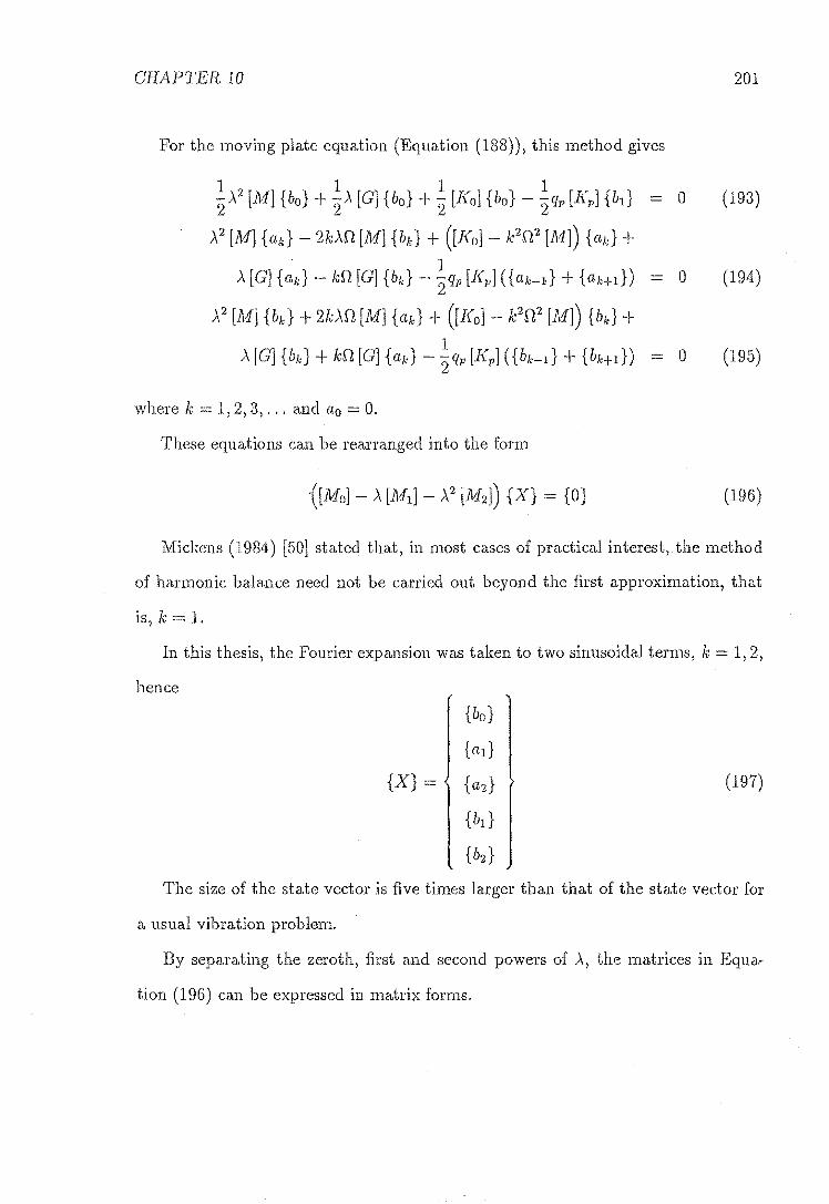
CHAPTER 10 201
For the moving plate equation (Equation (188)), this method gives
12111 "2.\ [NI1 {ba} +"2.\ [G1 {ba} + "2 [Ka1 {ba} - "2 Qp [Kp1 {bd - 0 (193)
.\2 [M] {ad - 2k.\n [M1 {bd + ([I{a1- k2n 2 [1\11) {ak} +
.\[G]{ad-kn[G]{bd-~qp[Kp]({ak_l:}+{ak+d) - 0 (194)
.\2 [1111 {bk } + 2k.\n [M] {ad + (rKa1- k2D,2 [111]) {b k } +
.\[G]{bd+kn[G]{ad-~qp[Kp]({bk-d+{bk+l}) == 0 (195)
where k = 1,2,3, ... and aa = O.
These equations can be rearranged into the form
(196)
Mickens (19811) [50] stated that, in most cases of practical interest, the method
of harmonic balance need not be carried out beyond the first approximation, that
is, k 1.
In this thesis, the Fourier expansion was taken to two sinusoidal terms, k = 1,2,
hence
{ba}
{ad
{X} = {a2} (197)
{bd
{bz}
The size of the state vector is five times larger than that of the state vector for
a usual vibration problem.
By separating the zeroth, first and second powers of A, the matrices in Equa-
tion (196) can be expressed in matrix forms.

CHAPTER 10 202
For the case when [G] = 0 (Equation (187))
[I<o] 0 0 -qp [I<p] 0
0 [I<lJ [I<p] 0 0
[lHo] 0 -~qp [I<p] [I<2] 0 0 (198)
!qp [I<pJ 0 0 [I<1] ~qp [I<p]
0 0 0 -~qp [I<p] [I<2J
where
[I<1] = [Ko] n 2 [A1] , [K2 ] = [I<01 4n2 [J\1]
0 0 0 0 0
0 0 0 2n[M] 0
[1\11] = 0 0 0 0 4n [A1J (199)
0 [lVf] 0 0 0
0 0 -4n [lVf] 0 0
[Ji1] 0 0 0 0
0 [M] 0 0 0
[A12 ] 0 0 -[M] 0 0 (200)
0 0 0 [M] 0
0 0 0 0 - [AI]
For the moving plate case (Equation (188))
[I<o] 0 0 [I<p] 0
0 [I<1] -~qp [I<p] -n[G] 0
[Mo]- 0 ~qp [I<p] [I<2] 0 -2n[G] (201)
-~qp [I<p] n[G] 0 [I<1] ~qp [I<p]
0 0 2n[G] -~qp [I<p] [[(2]

CHAPTER 10 203
- [G] 0 0 0 0
0 -[G] 0 2ft [AI] 0
[AIl] 0 0 [G] 0 4ft [AI] (202)
0 -2n [AI] 0 - [G] 0
0 0 [M] 0 [G]
- [AI] 0 0 0 0
0 -[M] 0 0 0
[M2] 0 0 [ AI] 0 0 (203)
0 0 0 -[M] 0
0 0 0 0 -[AI]
Equation (196) is a quadratic eigenvalue problem and the method of obtain
ing the eigenvalues and the eigenvectors is the same as the method described in
Section 8.3.2.
conditions for which the system becomes unstable under parametric exci
tations can be best represented on a stability chart, or sometimes referred to as a
Strutt diagram, where the instability regions in the frequency-amplitude space of
the excitation are plotted.
Takahashi's method for plotting the unstable regions seemed to be by inspec
tion of the real part of the eigenvalues for a range of excitation frequencies and
amplitudes.
Recently, a variation of the harmonic balance method, the incremental harmonic
balance method, has been developed to solve several problems in nonlinear dynam
ics [24,62]. This method is more suited for computational work than the classical
harmonic balance method, however, insight into the method of solution is lost, be
cause the problem of solving the governing differential equations is replaced by that
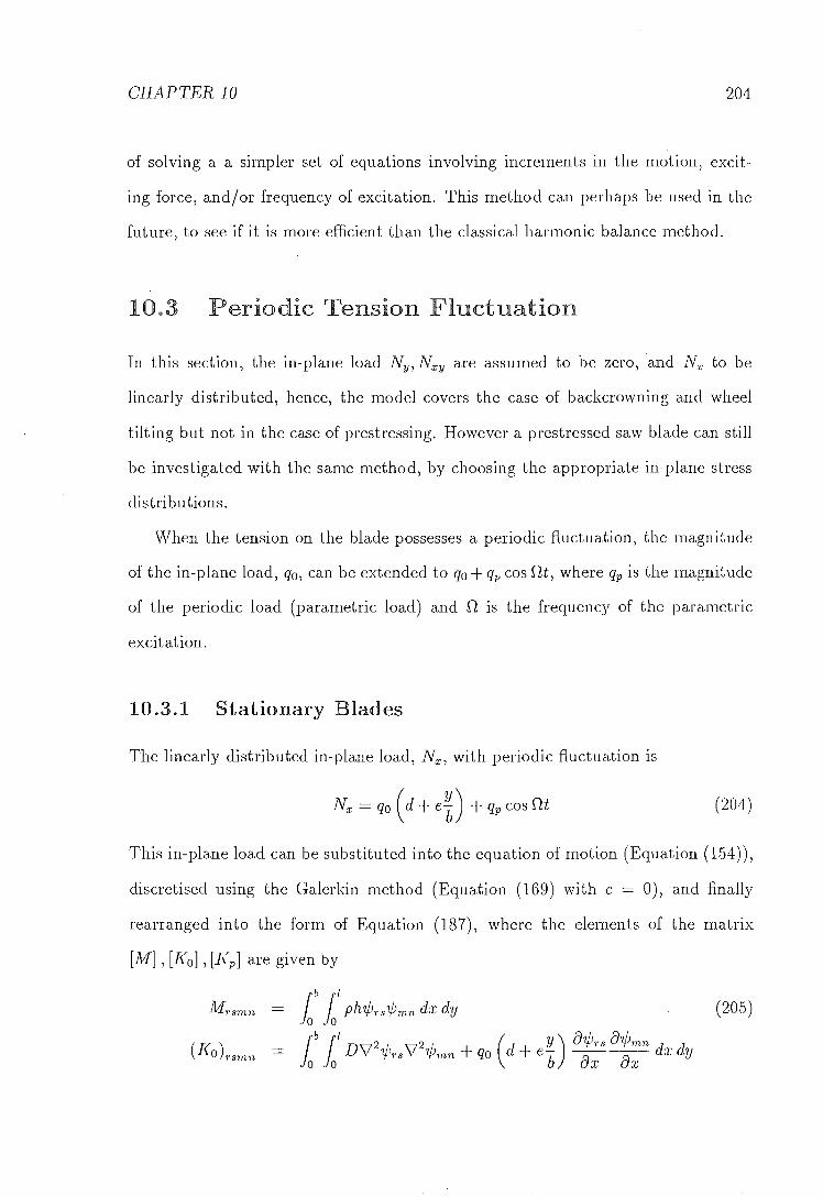
CHAPTER 10 204
of solving a a simpler set of equations involving increments in the motion, excit-
ing force, and/or frequency of excitation. This method can perhaps be used in the
future, to see if it is more efficient than the classical harmonic balance method.
10.3 Periodic Tension Fluctuation
In this section, the in-plane load Ny, N xy are assumed to be zero, and Nx to be
linearly distributed, hence, the model covers the case of backcrowning and wheel
tilting but not in the case of prestressing. However a prestressed saw blade can still
be investigated with the same method, by choosing the appropriate in-plane stress
distri bu tions.
When the tension on the blade possesses a periodic fluctuation, the magnitude
of the in-plane load, qo, can be extended to qo + qp cos nt, where qp is the magnitude
of the periodic load (parametric load) and n is the frequency of the parametric
excitation.
10.3.1 Stationary Blades
The linearly distributed in-plane load, N x , with periodic fluctuation is
N x = qo ( d + e~) + qp cos nt (204)
This in-plane load can be substituted into the equation of motion (Equation (1.54)),
discretised using the Galerkin method (Equation (169) with c = 0), and finally
rearranged into the form of Equation (187), where the elements of the matrix
[111] , [Ko] ,[Kp] are given by
1I1rsmn (205)

CHAPTER 10 205
(206)
(207)
where 1jJ are the trial functions. The subscripts r, 5, rn, n are as explained in Sec-
tion 7.5.1.
The harmonic balance method, Equations (196,198,199,200), can now be used
to obtain the instability regions for various excitation frequencies and amplitudes.
Numerical results were obtained for a blade with dimensions 0.22x 0.00l65x 0.8 m,
and with a uniform tension of 15000 N. The natural frequencies of this blade were:
III h 44.8 Hz for the first transverse mode.
It 12 = 53.2 for the first torsional mode.
"" h 91.8 Hz for the second transverse mode.
III 14 = 108.4 for the second torsional mode.
The mode shapes were plotted in Figure 73.
For the first transverse mode (1 x 1 trial function in the Galerkin solution), the
instability regions, obtained from a one-term Fourier expansion in the harmonic
balance step, were plotted on a Sh'utt diagram as shown in Figure 90.
Strutt diagram shows that the primary region of instability was at an exci-
tation frequency of twice the natural frequency of the blade, referred to as the 2h
simple parametric resonance. There was also a secondary region of instability at
n 11, referred to as the h simple parametric resonance.
Figure 91 shows the same instability problem with two-term Fourier expa.nsion in
the harmonic balance step. The primary instability region was the same as obtained
from the one-term Fourier expansion calculation, whereas the width of the .ft simple

CHAPTER 10 20G
Magnitude (kN/m) 80 .-----------~~~-~~------~~~~~~~~~.~~~_r~
60
40
20
O~------~--______ _L_+------~------~~--~---L------~ Q 20 40 f, 60 80 2fl 100 120
Frequency of Excitation (Hz)
Figure 90: Instability regions for the first transverse mode of a stationary blade subjected to
fluctuating tensions, with a one-term Fourier expansion.
parametric resonance region was much narrower than that from the one-term Fourier
calculation. There were regions of instability associated with 2/3f1 and 1/2JI, which
are sometimes referred to as the sub-harmonic resonances of the first mode.
These results showed that an increase in the number of terms, taken for the
Fourier expansion of the harmonic balance method, would result in an increase in the
number of the sub-harmonic resonance regions. However, the width of these regions
would be narrow. In practice, these sub-harmonic resonance regions are likely to
be insignificant due to the presence of damping, except when the amplitudes of the
excitation are very high.
Similar Strutt diagrams can be obtained for the other modes, and the primary
instability regions will always be the 2fn simple parametric resonance regions.
Figure 92 shows a Strutt diagram obtained for a 2x2 trial function Galerkin
solution. This diagram showed that for a blade subjected to fluctuating tension,

CHAPTER 10 207
o 20 40 60 80 100 120
Frequency of Excitation (Hz)
Figure 91: Instability regions for the first transverse mode of a stationary blade subjected to
fluctuating tensions, with a two-term Fourier expansion,
combination parametric resonances were nol possible, and each 2fn simple para-
metric xesonance could be calculated independently and then be superimposed on
the same Strutt diagram to represent the regions of instability of the blade.
Parametric resonances only occur through the non-zero terms in the matrix [Kp],
and for this case, [Kp] was diagonal, hence only the simple parametric resonances
were possible.
10.3.2 Moving Blade
in-plane load for a moving plate is the same as for a stationary plate with an
extra term added to take into account the effect of the straining device
(208)

CHAPTER 10 208
Magnitude (kN/m) 80 n-~~~~--~~~~
60
40
20
o 20 40 60 80 100 120 140
Frequency of Excitation (Hz)
Figure 92: Instability n;J-!.:'Vll" for a 2x2 trial function Galerkin solution of a stationary blade
subjected to fluctuating tensiolls, with a two-term Fourier expansion.
Applying the Galerkin method to the governing differential equation and re
arranging it to the form of Equation (188) where the coefficients of the matrices
are
A1rsmn
Grsnln
(K ) -P rsmn -
elt ) a'l/Jrs arj;mn b ax ax
(209)
(210)
(211 )
(212)
The harmonic balance method can again be used on Equation (188) to give the

CHAPTER 10 209
quadratic eigenvalue Equation (196) with the matrices [1\10] , [1\11 ] ,[1112] as given by
Equations (201, 202, 203).
The effects of transport speed are the inclusion of the centripetal term and the
Coriolis term in the governing equation.
The centripetal term is the - (1 "1) fJ~:n in the matrix [I<o]. Therefore,
when "1 = 1, as for the counterweight straining mechanism, the centripetal term does
not affect the saw blade. However, if it was present ("1 =1= 1), this term would have
a destabilising effect on the blade, by increasing the size of the instability regions
[58].
The Coriolis term is included in the matrix [0], and an inspection of this matrix
would help in understanding the results. [0] is a skew symmetric matrix, and for a
2 x 2 trial function Galerkin solution, it is of the form
[(~ -
o
o
o
o
o
0 31 0 0 0
o 0 42 0 0
(213)
This matrix showed that the 1 x 1 or 1 X 2 trial function Galerkin solution could
not account for the Coriolis term, because [0] [0] . The mimimum requirement was
a 2x1 function Galerkin solution, which could accurately predict the first natural
frequency of a moving blade.
Figure 93 shows the Strutt diagram" for a moving blade, with a transport speed
of 40 m/s. As the the transport speed increased, the first natural frequency of the
blade decreased, therefore, the 2f1 parametric resonance region also shifted down
the frequency axis. There were other regions of instability at higher amplitudes of
parametric excitation.
Naguleswaran and Williams (1968) [58], and Wu and Mote (1986) [95] showed

CHAPTER 10 210
Magnitude (kN/m) 60 .--------............... ~ .. .
50
40
30
20
10
a o 20 40 60 80 100
Frequency of Excitation (Hz)
Figure 93: Instability regions for a 2xl trial function Galerkin solution of a moving blade, with
c = 40 mis, subjected to fluctuating tensions, with a two-term Fourier expansion.
that the Coriolis term stabilised the blade by reducing the width of the instability
regions. This effect is shown in Figure 94, where the slope of the boundaries of
the 211 parametric resonance region are plotted against the transport speeds. As
the transport speed increased, the slope of the instability boundary increased, that
is, the area of the instability region decreased. However, Figure 93 shows that at
large amplitudes of tension fluctuation, other regions of instability appeared close
to the primary region of instability, therefore, the width of this region was actually
larger than expected. These extra regions of instability had not been discussed ill
previous publications, perhaps, beccLUse their methods of analysis were only for E)mall
amplitudes, whereas in this thesis, the harmonic balance method was used, which
could be applied to amplitudes of parametric excitation.

CHAPTER 10
Slope (Thou:;a.nd!:l) Frequency (Hz) o r--·~-····:--------~--------------------------------------,50
40 -2
'0 0""
30
20
-6 10
Slope
'LJ" Frequency
_8L __________ i-________ -L ________ ~ __________ L_ ______ ~0
o 20 40 60 80 100
Speed (m/s)
211
Figure 94: Inclination of the left boundary of the 211 simple parametric resonance region versus
transport speeds, c,
10.4 Periodic Tangential Cutting Forces
\VU and Mote (1986) [95].stated that' cutting forces in bandsaws possess periodic,
in-plane edge loading components potentially inducing combination parametric in-
stabilities'. However, they only discussed the in-plane normal periodic load due to
the feeding force of the timber into the blade. They concluded that simple torsional
parametric resonances and combination transverse-torsional parametric resonances
could be excited, but simple transverse, combination transverse-transverse, or com-
bination torsional- torsional parametric resonances could not.
As discussed in Section 9.6, the perpendicular component of the cutting force may
be much smaller than the tangential component. This section will, therefore, look
at the parametric instabilities of the blade due to a periodic tangential component
of the cutting force.

CHAPTER 10 212
The most significant periodicity of the tangential cutting force is from the fre-
quency of the teeth impa.cting the timber, hence, the angular frequency of the para-
mettic excitation Sl is equal to the blade axial speed e times the number of teeth per
unit length of the blade N, Sl - eN. However, Sl is usually very high (760 Hz for
the Waimak saw blade)' and therefore out of the range of parametric resonances.
10 .1 Stationary Blades
There has not been any application involving a stationary plate subjected to a
periodic tangential edge force, however, a study of this would provide more insight
into the plate problem.
In this section, only the cutting force qc was assumed to possess periodicity,
therefore, the in-plane loads were given as
Nx qo (d+e*) -(qc+qcpcosSlt) ~ (21 1) * (214)
N y 0 (215)
Nxy (qc+qcpcosSlt) (*r (216)
where qcp was the magnitude of the periodic component of the cutting force, and n was the frequency of the parametric excitation.
The Galerkin method could now be used to discretise the equation of motion to
the form of Equation (187) where
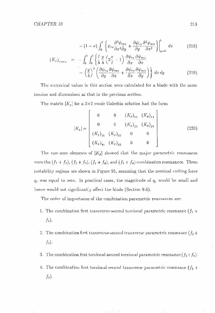
CHAPTER 10 213
_ (1- v) rt {V)rs cJ3'l/Jmn + a'l/Jrs a2'l/Jmn }Ib d;J;
io ax 2ay ay y=o (218)
_ rb rt {I y (2':' 1) a'l/Jrs a'l/Jmn io io b b I ax ax
(7.l)2 (a'l/Jrs a'l/Jmn + a'l/Jrsa'l/Jmn)} dx dy b ay ax ay (219)
The numerical values in this section were calculated for a blade with the same
tension and dimensions as that in the previous section.
The matrix [Kp] for a 2x2 mode Galerkin solution had the form
0 0 (Kp)13 (Kp)14
0 0 (Kp )23 (J(P)24 [Kp] = (220)
(Kp)31 (Kp)32 0 0
(Kp)41 (J(P)42 0 0
The non-zero elements of [Kp] showed that the major parametric resonances
were the (h + h), (f2 + h), (h + 14)' and (12 + 14) combination resonances. These
instability regions are shown in Figure 95, assuming that the nominal cutting force
qc was equal to zero. In practical cases, magnitude of qc would be small and
hence would not significantly affect the blade (Section 9.6).
The order of importance of the cornbination parametric resonances are:
1. The combination first transverse-second torsional parametric resonance (fI +
2. combination first transverse-second transverse parametric resonance (II +
/3).
3. combination first torsional-second torsional parametric resonance (12+14)'
4. The combination first torsional-second transverse parametric resonance (h +
/3).

CHAPTER 10
Magnitude (kN/m) 60 ~'~~~~----,
50
40
30
20
10
0~--------~~~--------~~~------4-~~~--------~
o 50 100 150
Frequency of Excitation (Hz) 200
214
Figure 95: Instability regions for a 2x2 trial function Galerkin solution of a stationary blade
subjected to periodic tangential cutting forces, with a two-term Fourier expansion.
These instability regions could also be obtained independently by considering
appropriate subsets of [Al], [Kol and [KpJ, which would be more feasible than illves-
tigating the total configuration.
10.4.2 Moving Blades
For moving plates) extra terms were added into the matrices to the governing
Equation (188). The components of the matrices in Equation (188) are
(221 )
Gr!nnn (222)
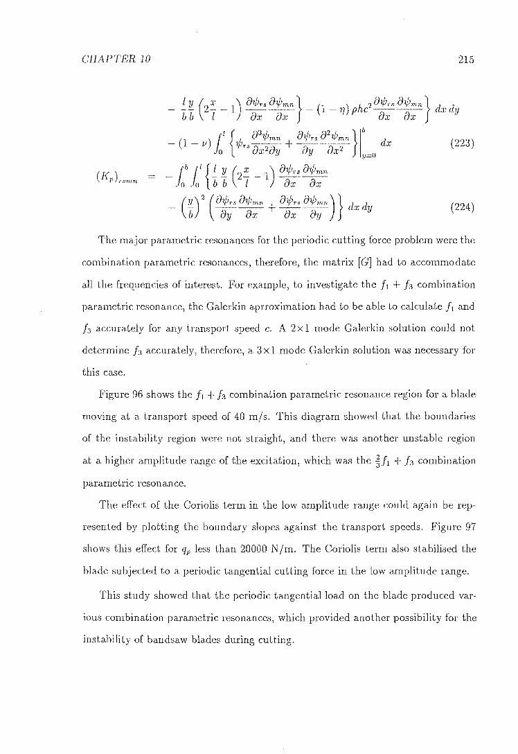
CHAP']'ER 10 215
(223)
(224)
The major parametric resonances for the periodic cutting force problem were the
combination parametric resonances, therefore, the matrix [G] had to accommodate
all the frequencies of interest. For example, to investigate the It + h combination
parametric resonance, the Galerkin aprroximation had to be able to calculate f1 and
h accurately for any transport speed c. A 2xl mode Galerkin solution could not
determine h accurately, therefore, a 3xl mode Galerkin solution was necessary for
this case.
Figure 96 shows the It + h combination parametric resonance region a blade
moving at a transport speed of 40 m/s. This diagram showed that the boundaries
of the instability region were not straight, and there was another unstable region
at a higher amplitude range of the excitation, which was the ~It + h combination
parametric resonance.
The effect of the Corio lis term in the low amplitude range could again be rep
resented by plotting the boundary slopes against the transport speeds. Figure 97
shows this effect for qp less than 20000 N 1m. The Coriolis term also stabilised the
blade subjected to a periodic tangential cutting force in the low amplitude range.
This study showed that the periodic tangential load on the blade produced var-
ious combination parametric resonances, which provided another possibility for the
instability of bandsaw blades during cutting.

CHAPTER 10 216
Magnitude (kN/m) 60 -~-~~~~~--~~~~~--~-~~~-rr~.
50
--~
40
30
20
10
OLI~~~~~~----L-------~~~~~------~.----~--~~~~
o 20 40 60 80 100 120 140
Frequency of Excitation (Hz)
Figure 96: Instability regions for a 2x2 trial function Galerkin solution of a moving bJade,
subjected to periodic tangential cutting forces, with a two-term Fourier expansion.
Slope (Thousands) Frequency (Hz) o .-~-~--------~- ......................... ~----------------------------, 160
140
-2 120
... ·"""·"····""·"",,0 .. ·.,, ·· .. ··[l· ...... ····"E} .....
·······················0
-4 -, 100
80
-6 60
40 -8
20
10 L-____ ~ ______ -L ______ 4-______ L-____ ~ ______ ~ ____ ~0
o 10 20 30 40 50 60 70
Speed (m/s)
Figure 97: Inclination of the left boundary of the h + h combination parametric resonance region
versus transport speeds, c.

er
ILITY OF AW
ES UND
o SERVAT
GFORC
11.1 nservative Problems
Elastic stability of nonconservative problems is yet another branch of the theory of
elasticity. The foundation of this subject was developed by Bolotin, who published
a book in Russian in 1961; it was translated to English in 1963 [11].
To illustrate the difference between conservative problems and nonconservative
problems, the behaviour of a cantilevered beam subjected to a unidirectionallongi
tudinal force is compared with that of a cantilevered beam subjected to a followeI'
force.
A cantilevered beam, subjected to a unidirectional compression, represents the
217

CHAPTER 11 218
Eigenvalue, A
Figure 98: Load versus frequency for a beam under unidirectional force.
classic Euler buckling problem. As the magnitude of the compressive force increases,
the fundamental natural frequency of the beam . The loa.d at which the
natural frequency becomes zero is the buckling load. type of buckling is referred
to as the diveTyent buckling or the static instability, which can be presented on
a plot of load versus natural frequency (Figure 98), or on a root-locus diagram,
where the complex roots of the equation of motion are traced as the load increases
(Figure 99). The equation of motion is usually manipulated to a matrix equation,
and the complex roots are its eigenvalues. For most stability problems, the imaginary
part of the eigenvalues, the natural frequencies, always come in pairs of positive and
negative values.
Figure 100 shows the action of a follower force on a cantilevered beam.
As the magnitude of the follower force increases, the fundamental natural fre
quency increases. The Euler buckling analysis would, therefore, predict that the
follower force stabilises the beam because the fundamental frequency would never
be equal to zero. However, a more advanced theory of elastic stability, the dynamic
method, would show that this system possesses a dynamic instability at a certain
magnitude of follower force. The dynamic instability can also be presented on a

CHAPTER 11 219
1m (A)
Figure 99: Root-locus diagram for a beam under unidirectional force.
q
Figure 100: Follower force on a cantilevered beam.

CHAPTER 11 220
Load I q
Eigenvaluei
A
Figure 101: Load versus frequency for a beam under follower force,
plot of the amplitude of the load versus the natural frequency (Figure lOlL or on a
root-locus diagram (Figure 102).
As discussed in Chapter 10) a dynamic instability occurs when the real part of
one or more eigenvalues become positive. On the load versus frequency plot, the
dynamic buckling load is the load at which an eigencurve reaches a maximum. On
the root-locus diagram, a dynamic buckling occurs when two natural frequencies
approach each other on the imaginary axis, which then turn 90 degrees and move
away from each other as the load increases beyond the buckling load.
The reason, as explained by Bolotin, that the Euler method cannot predict the
dynamic instability of the follower force is because the Euler method is only appli
cable for conservative problems. The follower force problem is a non conservative
problem.
The definition of a conservative force field is [49, page 32]
a field in which the work done in moving a particle Jrom point 1 to point 2
depends only on the position rl and r2 and is independent oj the path oj
integr'ation (Figure 103).

CHAPTER 11 1
Re(A}
Figure 102: Root-locus diagram for a beam under follower force.
2
Path A
r1 dr
Figure 103: Conservative force field.
-VV12c (2 F.dr = (2 F.dr Jrl Jrl
( 'J') e:) __ 0
~~
path A path B
The follower force problem can be shown to be nonconservative from the depen-
dency of the work done by the force on the manner in which the beam atLains its
final state. Figure 104 shows three ways in which the beam can reach a state defined
by a transverse deflection d and an angle of rotation 1> of the end section. In case
(a), rotation through an angle 1> with a subsequent displacement, the work done by

CHAPTER 11 222
(0). (c)
Figure 104: Three ways in which a beam attains its final state.
the force F is negative; in case (b), displacement with a subsequence rotation, the
work done is zero, and in case (c), rotation through an angle -¢, a displacement
and a final rotation through an angle 2¢, the work done is positive. This is one
feature inherent in all nonconservative problems.
11.2 Nonconservative Cutting Forces on Band
saw Blades
The cutting forces on a bandsaw blade are typically small [86], and, in the past,
were not considered to be the cause of instability of the bandsaw blade. Section 9.6
showed that for a typical bandsaw blade under a (unidirectional) tangential load,
the static buckling load was about 40 times the cutting load under normal condi
tions. Chapter 10 had considered the possibility that the instability was caused
by the periodic component of the tangential cutting force, however, the periodicity
of the cutting force had not been established. The dynamic instability due to a
nonconservative tangential cutting force was another possibility that had not been

CHAPTER 11 223
x
Figure 105: Follower tangential force on a saw blade.
considered previously.
The tangential cutting force on bandsaw blades can be shown to possess a non-
conservative property, by looking at the characteristics of the cutting process. There
are various cutting forces present in the cutting process, however, the largest force is
the one which opposes the motion of the saw tooth. It is obvious that this force will
always be tangential to the slope of the cutting edge of the blade as in Figure 105,
that is, a follower tangential force l.
Of course, if the blade is assumed to have small displacements, then the com-
ponent of the follower force perpendicular to the blade is small compared with the
component parallel to the equilibrium configuration of the blade. This is the as
sumption in the study of blades under tangential edge loads in Section 9.6. This
chapter excludes this assumption to see if the follower tangential cutting force can
alter the vibrational characteristics of the blade.
IThe term tangential force refers to the in-plane force parallel to a longitudinal edge of the equilibrium configuration of the blade, whereas, the term follower tangential force refers to the in-plane force tangential to a longitudinal edge of the vibrational configuration of the blade.

CHAPTER 11 224
z 1 qf I aw IZ~ aX
I
-~~~ x
y
--------x
Figure 106: Components of the follower force.
11.3 Formulation of Nonconservative Problems
The Hamilton's principle, described in Chapter 7 (Equation (53)), can be used to
formulate nonconservative problems, through the inclusion of the nonconservative
work done term.
The kinetic energy and the potential energy due to bending and due to in-plane
stresses are the same as those given in the previous chapters. The non conservative
work done can be found by considering the tangential cutting force. For simplicity,
assume that the force is uniform along the cutting edge of the blade, with a rnag-
nitude of qj force per unit length. The two components of this follower tangential
load are qj in the x direction (parallel to the plane of the plate) and qj 8wJ:,b) per-
pendicular to the plane of plate, where is the slope of the plate on the cutting
edge y = b.

CHAPTER 11 225
The component of the force parallel to the x-axis is conservative and has been
included in the in-plane stresses in Section 9.6. The contribution of the nonconser-
vativeness to the system is from the nonconservative work done by the perpendicular
component of this force. The variation of the nonconservative work done is given by
{I q] ~w DW dx Jo uX y=b
(226)
{b / q] ~w 1i (y _ b) Ow dx dy Jo Jo uX
(227)
where 1i (y - b) is a dirac delta function, which is equal to zero, except when y b.
This work done can be added into in the Hamilton's equation together with the
other energy terms (Section 9.6). The equation of motion is then given as
b) (228)
where
the boundary conditions are the same as for the conservative case (Equation (161)).
11. Method of Analysis
The method of analysis is the same as that for the conservative problems. Essentially,
the presence of a nonconservative force produces a non-self-adjoint boundary value
problem. A direct analysis of the non-self-adjoint problem is extremely difficult, and
an approximation method must be used in obtaining the solution. The most effective
approximation method for this case is the Galerkin method [11, page 58], even

CHAPTER 11 226
though the convergence of this method when applied to non-self-adjoint problems
has not been conclusively proven. However, it has been confirmed by experiments
and exact calculations that the form of loss of stability in the nonconservative cases,
can be successfully approximated by the first few modes of the natural oscillations.
The convergence of the Galerkin method can also be tested by a gradual increase
in the number of modes used in approximating the problem, and examining their
effects on the solution. If an increase in the number of modes does not alter the
solution by much, then it is likely that the solution has converged.
Abrahamsson and Siillstrom (1989) [1] applied a two-sided Ostrowski matrix
iteration to the eigenproblems of nonconservative continuous systems. For continu
ous beam systems, this method uses the exact solutions obtained from the dynamic
stiffness method, (Chapter 4) to solve the nonconservative cases, instead of using
predefined shape functions. However, this method does not offer any advantages to
the continuous plate problems because the exact solutions are difficult to obtain.
Leipholz and Pfendt (1982,1983) [43,441 studied the stability of rectangular plates
subjected to uniformly distributed follower forces, using the Galerkin method. These
studies closely resembled the bandsaw blade problem, and their method of analysis
was similar to the method used previously in this thesis. In fact, there was no special
technique required for the non conservative problem, as long as there was an eigen
solver which could handle non-self-adjoint problems; the PC-MATLAB eigen-solver
could.
More recently, Higuchi and Dowell (1989) [32] presented a study of a completely
free plate subjected to a nonconservative follower force, using the Rayleigh-Ritz
method. Even though, the method of discretisation differed from that in Leipholz
and Pfendt work, the treatment of the nonconservative element of the problem was
the same. These papers showed the same phenomena of dynamic instabilities as
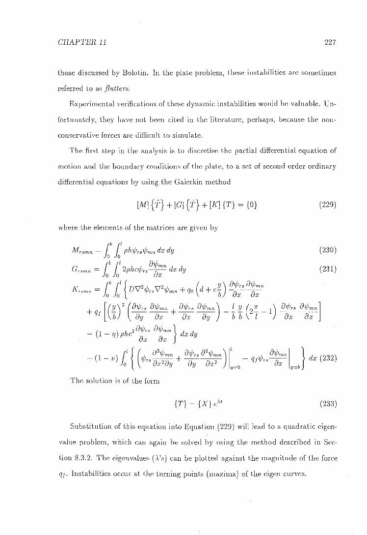
CHAPTER 11 227
those discussed by Bolotin. In the plate problem, these instabilities are sometimes
referred to as flutters.
Experimental verifications of these dynamic instabilities would be valuable. Un-
fortunately, they have not been cited in the literature, perhaps, because the non-
conservative forces are difficult to simulate.
The first step in the is to discretise the partial differential equation of
motion and the boundary conditions of the plate, to a set of second order ordinary
differential equations by the Galerkin method
[lit] {T} + [G] {T} + [K] {T} = {O} (229)
where the elements of the matrices are given by
(230)
(231)
1) o1jJrs 01jJmn] ax ax
The solution is of the form
{T} - {X} (233)
Substitution of this equation into Equation (229) will lead to a quadratic eigen
value problem, which can again be solved by using the method described in Sec-
tion 8.3.2. eigen values (A'S) can be plotted against the magnitude of the force
qf. Instabilities occur at the turning points (maxima) of the eigen curves.

CHAPTER 11 228
Table 21: First four frequencies (Hz) of a stationary blade subjected to a follower tangential load.
qj I 3 X 3 Functions I 4 X 4 Functions I 5 X 5 Functions I 0 44.8i 44.8i 44.7i
53.2i 53.1i 53.1i 91.8i 91.8i 91.8i
108.4i 107.9i 107.9i 30000 42.7i 42.8i 42.8i
62.4i 65.0i 65.3i 82.2i 79.1i 79.1i
111.4i 113.8i 117.7i
11.5 Results and Discussion
The numerical results in this section have been calculated for a blade with the same
dimensions and tension as that of Section 9.6 and Chapter 10.
11.5.1 Stationary Blades
Table 21 lists the first four natural frequencies of the blade at varIOUS maglll-
tudes of follower tangential edge load qj. The results were calculated with a 3 X 3,
4 X 4, and 5 x 5 trial functions in the Galerkin discretisation, which showed that the
3 X 3 function approximation could produce accurately the first four eigenvalues for
qj :=; 20000 N/m, while the results calculated with a 4x4 function approxima-
tion were practically the same as those calculated with a 5x5 function solution.
Although, these results were not proof of convergence for the Galerkin method in
nonconservative problems, they suggested that, for this application, the Galerkin
method appeared to converge to a unique set of solutions as the number of trial
functions increased.
Figure 107 shows the eigencurves for the 4 X 4 function calculations.
The nonconservative nature of the tangential load stabilised the first mode of

CHAPTER 11 229
1gencurves
Load (kN/m) 40~--~--~~~------------------------------------------~
o 20 40 60 80 100 120
Eigenvalues (Hz)
Figure 107: Eigencurves for a stationary blade subjected to a follower tangential edge load.
vibration, because at 30000 N 1m tangential load, the first frequency for the con-
servative case was 30.4 Hz (Table 19), whereas for the non conservative case, it was
42.S Hz.
The interesting dynamic instabili ty) discussed by Bolotin et.al., occurred when
the second (first torsional) natural frequency approached the third (second trans
verse) natural frequency as qj increased to approximately 32000 N/m. Even though,
this flutter load was very high compared with the usual cutting load, and was of the
same order of magnitude as the conservative buckling load (::::::::40000 N/m), the form
of loss of stability was very different from that found in the conservative case. ,This
type of instability on the bandsaw blade due to a tangential cutting force has not
been discussed previously, therefore, experimental studies are required to verify the
theoretical results presented in this chapter. However, these results were as expected
for the nonconservative case.

CHAPTER 11 230
Figure 108: First three modes of a blade subjected to 20000 N/m follower tangential load, with a
3x 3 trial function Galerkin solution.
The first three mode shapes of the blade, subjected to 20000 N /m follower tan-
gential load, are in Figure 108, which illustrates the effect of a follower tangential
load on the blade. Figure 109 shows the first mode and the unstable mode of the
blade at 36200 N/m load. The unstable mode was the combination of the first
torsional mode and the second transverse mode.
11.5.2 Moving Blades
Table 22 shows the first four eigenvalues2 of a blade subjected to three different
follower tangential loads qj, for various transport speeds c.
2The eigenvalues have been divided by 21f so that the imaginary parts represent the natural frequencies in Hz, therefore, the actual damping factors are 211" times the real part of the listed numerical values.
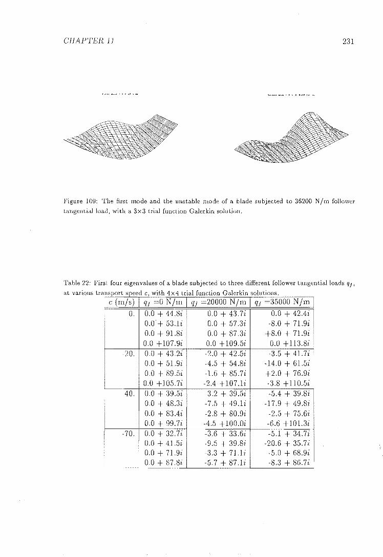
CHAPTER 11 231
Figure 109: The first mode and the unstable mode of a blade subjected to 36200 N 1m follower
tangential load, with a 3x3 trial function Galerkin solution.
Table 22: First four eigenvalues of a blade subjected to three different follower tangential loads q" at various transport speed c, with 4 x 4 trial function Galerkin solutions.
[ c (m/s) I q! =0 N/m I q! =20000 N/m I q! =35000 N/m I o. 0.0 + 44.8i ! 0.0 + 43.7i 0.0 + 42.4i
0.0' + 53.1i 0.0 + 57.3i -8.0 + 71.9i 0.0 + 91.8i 0.0 + 87.3i +8.0 + 71.9i 0.0 +107.9i 0.0 + 109.5i 0.0 + 113.8i
20. 0.0 + 43.2i -2.0 + 42.5i -3.5 + 41.7i • 0.0 + 51.9i -4.5 + 54.8i -14.0 + 61.5i 0.0 + 89.5i -1.6 + 85.7i +2.0 + 76.9i 0.0 +105.7i -2.4 +107.1i -3.8 +110.5i
-40. 0.0 + 39.5i -3.2 + 39.5i ! -5.4 + 39.8i 0.0 + 48.3i -7.5 + 49.li 7.9 + 49.8i 0.0 + 83.4i -2.8 + 80.9i .5 + 75.6i 0.0 + 99.7i -4.5 + 100.Oi -6.6 + 101.3i
-70. 0.0 + 32.7-£ -3.6 + 33.6i -5.1 + 34.7i 0.0 + 41.5i -9.5 + 39.8i -20.6 + 35.7i 0.0 + 7l.9i -3.3 + 71.li -5.0 + 68.9i
•
0.0 + 87.8i -5.7 + 87.li -8.3 + 86.7i
CHAPTER 11 232
These results show a very interesting phenomenon, which is the presence of damp
ing in the natural frequencies of the moving blade subjected to follower tangential
loads. If the transport speed c is positive, that is, the blade travels in the same
direction as the tangential load, then the real part of the eigenvalues are positive,
fortunately, this case is not possible in practice.
The dynamically unstable mode, found in the stationary blade analysis, also
occurred in this moving blade case, but at a higher qj, because of the damping. The
behaviour of the eigenvalues with a gradual increase in qj can be best represented
on a root-locus diagram. Figure 110 shows the root-locus diagram of a blade with
c =40 mis, and a 4x4 function Galerkin solution. The third eigenvalue was the
one responsible for the dynamic instability of the moving blade, while the second
eigenvalue was stabilised by the follower tangential force (large damping factor).
Because the nature of the cutting forces had not been well established, no specific
conclusion could be made about the stability of bandsaw blades during cutting.
However, this chapter illustrated a mechanism for the dynamic instability of the
blade due to a follower tangential cutting force. Because these results are presented
for the first time, their validity is questionable, however, they appeared to agree
with all the work published in the field of non conservative problems, and they also
make physical sense.

CHAPTER 11
Root- 0 US Diag
lsr Ji;ig. : :
80 .. ~ ... 2~~.~~~~: ................................ \ ................... j ............ ~ ................. . --¥- 3rd Elg. :: "'~
· . · . · . · . 60 ................................. ..
40 ._-....... ........,. ................ ..
..... ; .......... , ........ : ................... : ................ , .. _ ............... . . . . . 20 · . · .
o~. ________ L-______ -L ________________ -L ________ ~ ______ ~
-50 -40 -30 -20
Real 10 o 10
233
Figure 110: Root-locus diagram for the the first three eigenvalues of a blade, at c =40 m/s.

Chapter
CO CLUSIO
12.1 Summary
The work presented in this thesis can be summarised as follows:
12.1.1 Analysis of Structural Vibrations
The dynamic stiffness method was used in developing a computer program to solve
general three dimensional structure problems, consisting of thin beams, thick beams,
concentrated masses, gyroscopic rotors, springs, and viscous dampers.
A unique feature of this program was the inclusion of gyroscopic rotors, and
viscous dampers. This feature involved the use of complex arithmetic, and the search
for complex natural frequencies. The Muller's method was successfully employed
in the search for the real and complex natural frequencies of the systems under
investigation. In general, the Muller's method should have converged to a root
closest to the starting values, unfortunately, it was not always the case.
The modeshape of the system at a given frequency could be plotted by the
computer program, which had provided a useful tool for visualising the vibrational
234

CHAPTER 12 235
characteristics of the system.
This program had been used to study the Waimak bandsaw structural vibrations.
12.1.2 Structural Bandsaw
Experimental and theoretical analysis of the Waimak bandsaw revealed the following
vibrational characteristics:
• The structure of the bandsaw below the base contributed two low natural
frequencies of vibration at 30 Hz and 36 Hz. The dynamics of the shaft were
the major contribution to these two frequencies. If it were necessary to shift
these frequencies, an alteration to the shaft dimensions would be required. It
was not, however, a practical consideration for the existing bandsaws, but on
a new bandsaw design, this information may be of use.
" The structure above the base contributed two low natural frequencies at 9 Hz
and 21 Hz. The major contribution to the 9 Hz was a torsional mode of
the main column, and to the 21 Hz it was to-and-fro transverse vibration
of the main column. Because the rotating speed of the pulley was about
8 Hz, the 9 Hz torsional natural frequency was undesirable, and therefore, it
should be increased by adding extra stiffeners to the web of the main column.
This alteration could be easily accomplished on the existing bandsaws. The
20 Hz frequency could also be increased by bracing the main column to the
foundation in the direction of the vibration. It was noted that the Waimak
bandsaw had previously been braced to the foundation, however, the brace was
positioned near the central axis of the torsional mode, hence it had a minimal
effect on the 9 Hz vibration.

CHAPTER 12 236
• The top pulley oscillated vertically at 3.8 Hz natural frequency, due to the
flexibility of the straining device. A large amplitude of oscillation correspond
ing to this 3.8 Hz frequency had been observed during starting-up, and during
cutting, which would cause large tension fluctuations on the bandsaw blade.
An increase in the frequency of oscillation would result in a decrease in the
amplitude, and this could be accomplished by reducing the leverage ratio of
the counterweight lever arm. However, an investigation would be necessary to
optimise the leverage ratio of the counterweight arm.
• The gyroscopic effects of the rotating pulleys did not affect the structural
natural frequencies at the present bandsaw operating speed.
• Under idling conditions, the bandsaw structure vibrated at 8 Hz and its har
monics. Mechanical looseness offered the best explanation for the presence of
those harmonics.
12.1.3 Boundary Conditions of Moving Bandsaw Blades
This thesis has shown that it was possible to solve the moving beam problem by
using the dynamic stiffness method. The explicit form of the dynamic stiffness
matrix was difficult to obtain, however, a numerical scheme has been successfully
applied to the formulation of the moving beam dynamic stiffness matrix.
This method had been used to investigate three cases: the differences between
simply-supported and clamped-clamped end conditions, the coupling effects of in
termediate supports, and the forced lateral vibrations of moving beams.
For a typical bandsaw blade configuration, the natural frequencies of the simply
supported end conditions were lower than those of the clamped-clamped end con
ditions, up to 14% difference was found for the fundamental frequency of a blade

CHAPTER 12 237
0.3 m in length. As the axial speed of the moving beam increased the difference in
the natural frequency decreased. Comparisons between the calculated results and
the experimental results showed that simply-supported conditions provided a bet
ter representation of the bandsaw blade end conditions than the clamped-clamped
conditions.
For an un tensioned three-span bandsaw blade, the coupling effects between the
spans were quite significant. For a saw blade under a typical level of tension, coupling
was small and the natural frequencies of each span could be calculated individually.
The coupling effects increased the single span natural frequencies only slightly. As
the axial speed of the beam increased, the coupling effects decreased.
Although, the 'mode shapes' of a moving beam were dependent on the direction
of axial motion of the beam, the resonance frequencies were not. A large amplitude
of transverse vibration would occur when the frequency of the transverse excitation
was close to the natural frequency of the moving beam, regardless the position of
the excitation.
12.1.4 Analysis of Plate
A procedure for solving plate problems, based on the Galerkin approximation, has
been developed in this thesis. Firstly, Hamilton's principle was used to obtain the
equation of motion and all the boundary conditions of a plate problem. Then,
the equation of motion and the boundary conditions were discretised into a set
of second order differential equations, or in the case of linear vibration, a set of
algebraic equations. Gaussian quadrature rule was used to perform the integration
required in the discretisation step, hence reducing most of the unnecessary hand
calculations. The program PC-MATLAB was then used in the final step of finding
the eigenvalues and the eigenvectors of the governing equation.

CIIAPTER12 238
This procedure has been extended to cover a wide range of applications, from
simple vibration problems to dynamic instability problems. The moving plate case
has also been solved by using this Galerkin approximation procedure.
12.1.5 Bandsaw
In-plane are very important in bandsaw blades, because they can alter
the saw blade performance considerably. This thesis considered the vibration of
saw blades subjected to: a uniform stress, a linear stress due to backcrowning and
wheeltilting, a parabolic stress due to prestressing, and stresses induced by uniform
tangential cutting forces.
For the uniform tension, the plate solutions were close to the solutions of a
beam under longitudinal tension. An advantage of the plate solutions over the
beam solutions was that it combined both the transverse and the torsional mode of
vibration, hence it would take care of coupling effects automatically. The solutions
for a moving plate under uniform tension were also close to those for a moving beam.
This thesis had shown that the effects of the wheel-tilting can be represented by
a linear stress distribution. Wheel-tilting results in a decrease of the first transverse
frequency and an increase of the first torsional frequency. A small amount of wheel
tilting would improve the performance of the blade, however, too much tilt would
destabilise the blade because of the low first transverse frequency.
The backcrowning process appeared to set up a linear residual stress distribution
across the width of the blade, and its effects were, therefore, similar to those obtained
from the wheel-tilting operation. An approximate equation had been used to cal
culate the magnitude of the residual stress induced from back-crowning. It showed
good agreement with the experimental results, however, more work is needed to test
the validity of this approximate solution for a wider range of backcrowning.

CHAPTER 12 239
The mam objective of prestressing was to set up a parabolic residual stress
across the width of the blade. The light-gap measurement technique had been
used to measure the amount of prestress, however, Foschi had concluded that this
method was unreliable. This thesis investigated the effects of parabolic residual
stress on bandsaw blade as an approximation to the prestressing process. The
effects found were an increase in the first torsional frequency and a slight decrease
in the first transverse frequency, which with the experimental results. Strictly
speaking, the parabolic residual stress in the longitudinal direction alone was not
adequate, because it would induce additional stresses in other directions. However,
these stresses were very difficult to incorporate into the polynomial stress functions
considered this thesis, they were, therefore omitted, but should be included in a
more complete study of stresses occurring in bandsaw blade.
A uniform tangential force along one edge was used to consider the effects of the
main cutting force on a bandsaw blade. The buckling force was found to be approx
imately forty times larger than the typical cutting force. For a moving blade the
buckling force decreased, but the decrease was insignificant compared to its magni
tude. Because the magnitude of the main cutting force at the onset of instability
has not been measured, it was impossible to draw any conclusions about the type of
instability occurring in the bandsaw blade. However, the results in this thesis
gested that the divergent buckling due to tangential cutting force seemed unlikely
to occur in practice.
12.1.6 Excitations on Blades
In this thesis, the harmonic balance method has been applied to the parametric exci
tations of a bandsaw blade. Two cases of parametric excitation have been examined:
the periodic fluctuations in tension, and the periodic tangential cutting force.

CHAPTER 12 240
For the periodic fluctuations in tension, no combination parametric resonance
was possible. The major regions of dynamic instability were the 2fn simple para
metric resonance regions) which had been predicted from the beam modeL For a
moving blade, a Coriolis term, and a centripetal term were added to the equation
of motion for a stationary blade. However, the centripetal term was eliminated
because the straining device was a counterweight mechanism, therefore, only the
Coriolis term was included. The Coriolis term stabilised the parametric resonances
of the blade by reducing the width of the instability regions. At large amplitudes
of excitation, other regions of instability were present) which increased the areas of
instability. These additional instability regions had not been presented previously,
perhaps, because the methods of investigation had been for small amplitudes of ex
citation only. The harmonic balance method allowed large amplitudes of excitation
to be investigated.
The periodic tangential cutting force on the blade produced interesting combina
tion parametric resonances, while the simple parametric resonances became insignif
icant. The important parametric resonances were the combination first transverse
second torsional, first transverse-second transverse, first torsional-second torsional,
and first torsional-second transverse parametric resonance. For a typical bandsaw
blade configuration, these regions of dynamic instability were close to each other,
and therefore) at a certain magnitude of excitation, they merged together to produce
a large region of instability. Conclusions similar to those for the stationary blade
have been drawn for the moving blade case.
12.1.7 Nonconservative Cutting Forces on Bandsaw Blades
The tangential cutting force had been shown to possess a nonconservative property.
The theoretical investigation into the nonconservative problems has revealed another

CHAPTER 12 241
interesting type of dynamic instability. As the magnitude of the tangential load
increased, the first transverse natural frequency decreased slightly, the first torsional
frequency increased, and the second transverse frequency decreased. When the
first torsional frequency approached the second transverse frequency, they became
dynamically unstable, because one of the eigenvalues contained a positive real part.
The magnitude of the buckling load in this case was less than that in the conservative
problem, however, it was still very high compared with a typical cutting load.
For the moving blade case, damping was produced by the non conservative load,
because all the eigenvalues possessed negative real parts. The magnitude of the
buckling load was, therefore, increased as the transport speed of the blade increased,
and the frequency which was responsible for the instability was the second transverse
frequency.
12.2 Future Work
work presented in this thesis has covered a wide range of disciplines in the
bandsaw vibration field. Therefore, it is necessary, in the future, to direct efforts to
more specific areas of interest, so that greater confidence can be associated with the
results of the present analyses.
The following suggestions are arranged in the order of their importance.
12.2.1 Mechanism of Cutting Wood
The mechanism of cutting wood is believed to be the most important topic in wood
machining at present. It will provide useful information for studying the behaviour
of the present saw blades as well as for developing new methods of cutting wood.
An experimental study would be best carried out in a laboratory environment.

CHAPTER 12 242
A testing machine should consider the following items:
41 Isolation of one tooth cutting action.
Variety of tooth profiles.
High speed photography.
,. Accurate measurements of various cutting forces .
• Precise adjustment of the cutting speed, and the depth of cut.
A theoretical consideration can, perhaps, follow by modelling the cutting action,
or the energies transferred during the cutting process.
12.2.2 In-Plane Stress Measurement Techniques
As indicated in this thesis, the present methods of measuring residual stresses in a
bandsaw blade are not reliable, a better non-destructive technique would, therefore,
be very valuable. It would assist the Saw Doctors in optimizing the performance
of the saw blade, as well as the researchers in finding better ways of improving the
blade.
This development, perhaps, will not be perfected in the near future. In the
mean time, e'X,})erimental investigation on the accuracy of the present techniques
would be quite feasible. For example, the measurements of prestress using the light
gap technique could be compared with the direct measurements from using strain
gauges.
CHAPTER 12
12 .3 Parameters
during Cutting
243
to the Instability of Saw
The instability of bandsaw blades during cutting is the most critical factor in limiting
the rate of production, it is, therefore, necessary to investigate the cause of this
instability. The mechanism of cutting wood and the measurement of cutting forces
should be the prerequisite for this instability investigation. The theoretical method
presented in this thesis should be adequate for the verification of the experimental
results.
12 Straining Devices
In-plane stresses playa major part in the stability of bandsaw blades, of which, the
static tension provides the highest stress level. The straining device is, therefore, a
very important part of the bandsaw. Modern bandsaws have used air or hydraulic
straining mechanisms, instead of the counterweight mechanism. However, the ad
vantages of these modern straining devices have not been discussed, and from the
theoretical point of view, they are less favourable than the previous counterweight
mechanism (due to the presence of the centripetal term in the equation of motion).
Perhaps, an active control of bandsaw vibrations can be achieved through the
straining device.

A dge
I would like to thank Professor H. McCallion, my supervisor and the Head of the
Mechanical Engineering Department, for his assistance and guidance throughout
this research. I am also grateful to Dr. R.I. Astley and Mr. B. Donohue for their
interest and assistance.
Acknowledgement is also due to: Mr. G. J\.1cGill, for proof-reading this thesis
and for making many valuable constructive criticisms; Mr. M. Minan/, for assisting
with the experimental work; Afr. P. Smith, for helping ·with the computer facility;
and to all my postgraduate colleages, in particular Dr. NI. Aitken, for discussing
and giving helpful advice on this research.
Appreciation is extended to: the University Grants Committee, for their finan
cial assistance; the Southern Industrial Development Division, for the use of their
equipment; the Waimakariri Sawmill, for allowing access to their bandsaw; and the
Southern Cross Engineering Company, for providing invaluable information on the
design of their bandsaws.
I also wish to thank all my family, whose encouragement was very much appreci
ated. Last, but not least, I am indebted to my fiancee, Thu Hong, for her continued
patience and encouragement throughout this research.
244

re
[1J T.J.S.Abrahamsson and J.H.Sallstrom 1989 International Journal for Numer
ical1l1ethods in Engineering 28) 1827-1837. Eigensolutions of non-conservative
continuous mechanical systems computed by use of a matrix iteration method.
[2) D.Afolabi 1987 Computers and Structures 26, 1039-1040. Linearisation of the
quadratic eigenvalue problem.
[3J F.E.Allen 1985 Proceedings of the Eigth International Wood 1I1achining Semi
nar) Forest Products Laboratory} University of California, 384-404. High-strain
theory and application.
[4) F.E.Allen 1973 Australian Forest Industries Journal 39, 30-35. Quality control
in the timber industry.
(5) D.W.Alspaugh 1967 Journal of the Franklin Institute 283) 328-338. Torsional
vibration of a moving band.
[6] D.L.Anderson 1974 Natural Frequency of Lateral Vibrations of a 1I1ultipie Span
1I10ving Band Saw. Vancouver: Western Forest Products Laboratory.
[7] S.T.Aria.ratnam and S.F.Asoka.nthan 1988 Journal of Vibration} Acoustics)
Stress} and Reliability in Design, Transactions of the ASlvIE 110, 350-355.
Torsional oscillations in moving bands.
245

CHAPTER 4 246
[8] S.F.Bassily and S.M.Dickinson 1975 lournal of Applied Mechanics) Transac
tions of the ASlJIE 42, 858-863. On the use of beam functions involving free
edges.
[9] R.B.Bhat 1985 lournal of Sound and Vibration 102, 493-499. Natural fre
quencies of rectangular plates using characteristic orthogonal polynomials m
Rayleigh-Ritz method.
[10] R.E.D.Bishop and D.C.Johnson 1960 The Mechanics of Vibration. Cambridge:
Cambridge University Press.
[11] V.V.Bolotin 1963 Nonconservative Problems of the Theory of Elastic Stability.
Oxford: Pergamon Press.
[12] V.V.Bolotin 1964 The Dynamic Stability of Elastic Systems. San Francisco:
Holden- Day.
[13] R.L.Burden,J.D.Faires and A.C.Reynolds 1981 Numerical Analysis. Boston:
Prindle, Weber & Schmidt.
[14] R.D.Cook 1981 Concepts and Applications of Finite Element Analysis. New
York: John Wiley & Sons, Inc.
[15] G.R.Cowper 1966 loumal of Applied Mechanics) Transactions of the ASME
33, 335-340. The Shear Coefficient in Timoshenko's Beam Theory.
[16] C.D' Angelo III,N.T.Alvarado,K.W.Wang and C.D.Mote,Jr. 1985 Shock and Vi
bration Digest 17, 11-23. Current research on circular saw and band saw sta
bility.
[17] A.K.Das 1982 P.roceedings of the Seventh International Wood Alachining Sem
inar) Forest Product Labratory! University of California, 175-182. Analysis of

CHAPTER 4 247
dynamic stability of bandsaw systems.
[18] S.G.J. de Cock 1987 Transactions of the Institution of PTOfessional Engineers
New Zealand 14, 152-162. The role of experimental vibration analysis in product
development and machine diagnostics.
[19] S.M.Dickinson and A.D.Blasio 1986 Journal of Sound and Vibration 108,51-62.
On the use of orthogonal polynomials in the Rayleigh-Ritz method for the study
of the flexural vibration and buckling of isotropic and orthotropic rectangular
plates.
[20] J.J.Dongarra et.aL 1979 LINPACf( Users' Guide. Philadelphia: Society for
Industrial & Applied Mathematics.
[21] E.Downham 1957 The Engineer, 588-591. Theory of shaft whirling. No.lII
Influence of rotor inertia.
[22] E.Downham 1957 The Enginee1', 624-628. Theory of shaft whirling. No.IV-The
influence of asymmetry in bearing constraints on the whirling of a shaft and
rotor.
[23] D.J.Ewins 1984 lV[odal Testing:Theory and Practice. Letchworth: Research
Studies Press Ltd.
[24] A.A.Ferri 1986 Journal of Applied Mechanics, Transactions of the ASME 53,
455-457. On the equivalence of the incremental harmonic balance method and
the harmonic balance-Newton Raphson method.
[25] R.O.Foschi 1975 Wood Science and Technology 9, 243-255. light-gap tech-
nique as a tool for measuring residual stresses in bandsaw blades.

CHAPTER 4 248
[26J A.Gronlund 1988 Proceedings of the Ninth Intemational l1'ood .M~achining Sem
l:nm', For'est Products Laboratory) University of Califomia, 342-350. Measuring
and modelling of cutting forces-progress report on an ongoing project.
[27J W.Giittinger 1987 Intemational Series of Numerical l11athemal'ics 79, 98-113.
Bifurcation theory in physics: recent trends and problems.
[28J \\T.G.Halvorsen 1977 Sound and Vibmtion 11,8-20. Impulse technique for struc
tural frequency response testing.
[29J RD.Henshell, et.aL 1965 Proceedings of the Institute of Electrical Engineers
112, 2133-2139. Natural frequencies and mode shapes of vibration of trans
former cores.
[30J Hewlett-Packard 1982 The Fundamentals of Signal Analysis. Application Note
243, U.S.A.
[31J Hewlett-Packard 1983 Dynamic Signal Analyzer' Applications, Effective A;Ja
chineTY M~aintenance Using Vibmtion Analysis. Application Note 243-1, U.S.A.
[32] K.Higuchi and E.H.Dowell1989 Joumal of Sound and Vibmtion 132, 115-128.
Dynamic stability of a completely free plate subjected to a controlled non
conservative follower force.
[33J W.P.Howson 1985 Software fOT Engineering Problems. Adey, 27-36. A compact
method for computing the eigenvalues and eigenvectors of plane frames.
[34J C.S.Hsu 1963 Joumal of Applied Mechanics, Tmnsactions of the ASA1E 30,
367-372. On the parametric excitation of a dynamic system having multiple
degrees of freedom.

CHAPTER 4 249
[35] L.G.Jaeger 1964 Elementary Theory of Elastic Plates. Oxford: Pergamon Press,
Ltd.
[36] Y.I.Kim and B.Tabarrok 1972 Journal of the Fmnklin Institute 294 381-399.
On the nonlinear vibration of travelling strings.
[37] E.Kirbach and T.Bonac 1978 vVood and Fiber 9, 245-251. The effect of tension
ing and wheel tilting on the torsional and lateral fundamental frequencies of
bandsaw blades.
[38] E.Kirbach and T.Bonac 1978 Wood and Fiber 10,19-27. An experimental study
on the lateral natural frequency of bandsaw blades.
[39] F.Kozin and R.M.Milstead 1979 Journal of Applied lI1echanics, Tmnsactions
of the ASMB 46, 404-4:10. The stability of a moving elastic strip subjected to
random parametric excitation.
[40] G.Kron 1939 Tensor Analysis of Networks. New York: John \i\filey.
[41] G.Kron 1963 Diakoptics. London: Macdonald.
[42] H.L.Langhaar 1962 Energy }V{ethods in ApIJlied M~echanics . .\lew York: John
'Wiley & Sons, Inc.
[43] H.H.E.Leipholz and F.Pfendt 1982 Computer fl1ethods in Applied Mechanics
and Engineering 30, 19-52. On the stability of rectangular, completely sup
ported plates with uncoupling boundary conditions subjected to uniformly dis
tributed follower forces.
[44] H.H.E.Leipholz and F.Pfendt 1983 Computer kJethods in Applied 111echanics
and EngineeTing 37, 341-365. Application of extended equations of Galerkin

CHAPTER 4 250
to stability problems of rectangular plates with free edges and subjected to
uniformly distributed follower forces.
[45] A.\'V.Leissa, 1969 Vibmtion of plates. NASA SP-160.
[46] A.W.Leissa 1973 Journal of Sound and Vibmiion 31,
tion of rectangular plates.
. The free vibra-
[47] A.Y.T.Leung 1988 Journal of Sound and Vibmtion 124, 249-267. Inverse iter
ation for the quadratic eigenvalue problem.
[48] H.McCallion 1973 Vibmtion of Linea?' A1echanical Systems. London: Longman
Group Limited.
[49] L.Meirovitch 1967 Analytl:cal ~Methods in Vibmtions. New York: The Macmillan
Company.
[,50] R.E.Mickens 1984 Journal of Sound and Vibmtl:on 94, 456-460. Comments on
the method of harmonic balance.
[51] C.Moler,J.Little and S.Bangert 1987 PC-MATLAB User's Guide. The Math
Works, Inc.
[52] C.D.Mote,Jr. 1965 Journal of the Franklin Institute 279, 430-444. A study of
bandsaw vibrations.
[53] C.D.IVlote,Jr. and S.Naguleswaran 1966 Journal of Engineering for Ind'ustry,
Transactions of the ASME 88 151-156. Theoretical and experimental band saw
vibrations.
[54] C.D.Mote,Jr. 1966 Joul1wl of Applied Mechanics, Transactions of the AS!l1E
33, 46~)-464. On the nonlinear oscillation of an axially moving string.

CHAPTER 4 251
[55] C.D.Mote)r. 1968 Intemational Journal of Mechanical Science 10, 281-295.
Divergence buckling of an edge-loaded axially moving band.
[56] C.D.Mote)r. 1968 Joumal of the Franklin Institute 285, 329-346. Dynamic
stability of an axially moving band.
[57] C.D.Mote,Jr. and A.L.Thurman 1971 Journal of Applied Nfechanics) Transac
tions of the ASME 38) 279-280. Oscillation modes of an axially moving material.
[58] S.Naguleswaran and C.J.H.Williams 1968 Intemational Jom'nal of Mechanical
Science 10, 239-250. Lateral vibration of bandsaw blades, pulley belts and the
like.
[59] A.H.Nayfeh and D.T.Mook 1979 Nonlinear Oscillations. New York: \Viley
In terscien ceo
[60] G.Pahlitzsch and K.Puttkammer 1972 Holz als Roh- und Werkstoff30, 165-174.
The loading of bandsaw blades: Stresses and and strength factors.
[61] N .S.P almer and H.McCallion 1973 The Institution of Mechanical Engineers)
Applied A1echanics Group 187,63-70. Natural frequencies and mode-shapes of
systems of generally interconnected shafts.
[62] C.Pierre E.H.Dowell 1985 Joumal of Applied A1echanics) Transactions of
the AS~ME 52, 693-697. A study of the dynamic instability of plates by an
incremental harmonic balance method.
[63] W P.Flannery)S.A.Teukolsky and \V.T.Vetterling 1986 Numerical
Recipes: the Art of Scientific Computing. Ca.rnbridge: Cambridge University

CHAPTER 4 252
[64] \:V.H.Press,B.P.Flannery,S.A.Teukolsky and W.T.Vetterling 1988 Numerical
Recipes in C: the krt of Scientific Computing. Cambridge: Carnbridge U ni
versity Press.
[65] N.F.Rieger and H.McCallion 1965 International Journal of fl1echanical Science
7, 253-261. The natural frequencies of portal frames-I.
[66] N.F.Rieger and H.McCallion 1965 International Journal of Mechanical Science
263-276. The natural frequencies of portal frames-II.
[67] R.J.Roark and W.C.Young 1975 Formulas for Stress and Strain. Tokyo:
McGraw-Hill Kogakusha.
[68] A.D.Roberts and S.C.Lapidge 1977 Manufacturing Proccesses. New York:
McGraw-Hill, Inc.
[69] R.H.Russell and J.C.Deel1977 Sound and Vibration II, 22-38. Modal Analysis:
Trouble-shooting to product design.
[70] J.M.M.Silva and N.M.M.Maia 1988 Journal of Sound and Vibration 124,13-26.
Single mode identification techniques for use with small microcomputer.
[71] A .Simmond 1980 liVide Bandsaws, the A rt of Saw Doctoring. London: Stobart
& Son Ltd.
[72] S.K.Sinha 1988 JOltrnal of Sound and Vibration 128, 505-507. Comments on
"Dynamic stability of a rectangular plate subjected to distributed in-plane dy
namic force".
[73] R.Sklltch 1897 Annalen der Physik und Chemie 61,190-195. Ueber die Bewe
gung eines gespannten Fadens, welcher gezwungen ist, durch zwei feste Punkte

CHAPTER 4 253
mit emer konstanten Geschwindigkeit zu gehen und zwischen denselben m
Transversal-Schwingungen von Amplitude versetzt wird.
[74] B.T.Smith et.al1974 Mai1'ix Eigensystem Routines-EISPACf{ Guide. Berlin:
Springer.
[75] A.I.Soler 1968 Journal of the Franklin Institute 286, 295-307. Vibrations and
stability of a moving band.
[76] RSzilard 1974 Theory and Analysis of Plates. Englewood Cliffs, New Jersey:
Prentice-Hall, Inc.
[77] K.Takahashi 1981 Journal of Sound and Vibration 78,519-529. An approach to
investigate the instability of the multiple-degree-of-freedom parametric dynamic
[78] K.Takahashi and Y.Konishi 1988 Journal of Sound and Vibration 123, 115-
127. Dynamic stability of a rectangular plate subjected to distributed in-plane
dynamic force.
[79] C.A.Tan and C.DJvlote,Jr. 1988 Proceedings of the Ninth International Wood
1Iiachining Seminar) F01'est Product Laborat01'Y) University of Califomia, pg
266-285. Vibration analysis of a guided axially moving band.
[80] C.Tanaka,Y.Shiota,A.Takahashi and M.Nakamura 1981 Wood Science and
Technology 15, 145-159. Experimental studies on bandsaw blade vibration.
[81] C.Tanaka,Y.Shiota and A.Takahashi 1983 1110kuzai Gakkaishi 29, 308-314.
Bandsaw blade vibration during sawing.
[82] A.L.Thurman and C.D.Mote,Jr. 1969 Journal of Applied M~echanics) Transac-
tions of the A 36, 83-91. Free, periodic nonlinear oscillation of an axially

CHAPTER 4 254
moving strip.
[83] S.P.Timoshenko and J.N.Goodier 1970 Theory of Elasticity. New York:
McGraw-Hill.
[84] A.C.Ugural and S.K.Fenster 1981 Advanced Strength and Applied Elasticity.
London: Edward Arnold.
[85] A.G.Ulsoy and C.D.Mote,Jr. 1978 Shock and Vibration Digest 10, 3-15. Band
saw vibration and stability.
[86] A.G.Ulsoy and C.D.Mote,Jr. 1980 Wood Science 13, 1-10. Analysis of bandsaw
vibration.
[87] A.G.Ulsoy and C.D.Mote,Jr. 1982 J01lrnal of Engineering for Industry} Trans
actions of the ASlvIE 104, 71-78. Vibration of wide band saw blades.
[88] K.W.Wang and C.D.Mote 1986 Journal of Sound and Vibration 109, 237-258.
Vibration coupling analysis of band/wheel mechanical systems.
[89] K.W.Wang and C.D.Mote 1987 Journal of Sound and Vibration 115, 203-216.
Band/wheel system vibration under impulsive boundary excitation.
[90] P.M.vVare 1977 Ph.D. Thesis} University of Canterbury. An investigation into
the behaviour of rotating shaft systems incorporating oil film bearings and
gyroscopic effects.
[91] Wilkie Brothers Foundation Fundamentals of Band M·achining. Albany, New
York, Delmar.
[92] F.W.vVilliams and W.H.Wittrick 1970 International Journal of llifechanical Sci
ence 12, 781-791. An automatic computational procedure for calculating natu
ral frequencies of skeletal structures.

CHAPTER 4 255
[93] Ed M.Williston 1978 Saws: Design! Selection! Operation! Maintenance. San
Francisco: Miller Freeman Publications.
[94] W.Z.Wu and C.D.Mote,Jr. 1984 FOTest FTOducts JouTnal 34, 12-21. Analysis of
vibration in a bandsaw system.
[95] W.Z.Wu and C.D.Mote,Jr. 1986 Joumal of Sound and Vibration 110, 27-39.
Parametric excitation of an axially moving band by periodic edge loading.
[96] W.Z.Wu 1986 FTOceedings of the FouTth International Modal Analysis ConfeT
ence! Union College! Schenectady! New YOTk, 1621-1627. Modal analysis of a
moving band under cutting loads.
[97] D.Young 1950 Journal of Applied Mechanics! Transactions of the ASME 17,
448-453. Vibration of rectangular plates by the Ritz method.
[98] Yi-Yuan Yu 1964 The Journal of the Acoustical Society of AmeTica 36, 111-
120. Generalized Hamilton's principle and variational equation of motion in
nonlinear elasticity theory, with application to plate theory.
[99] O.C.Zienkiewicz and K.NIorgan 1983 Finite Elements and AppTOximation. New
York: John Wiley & Sons, Inc.
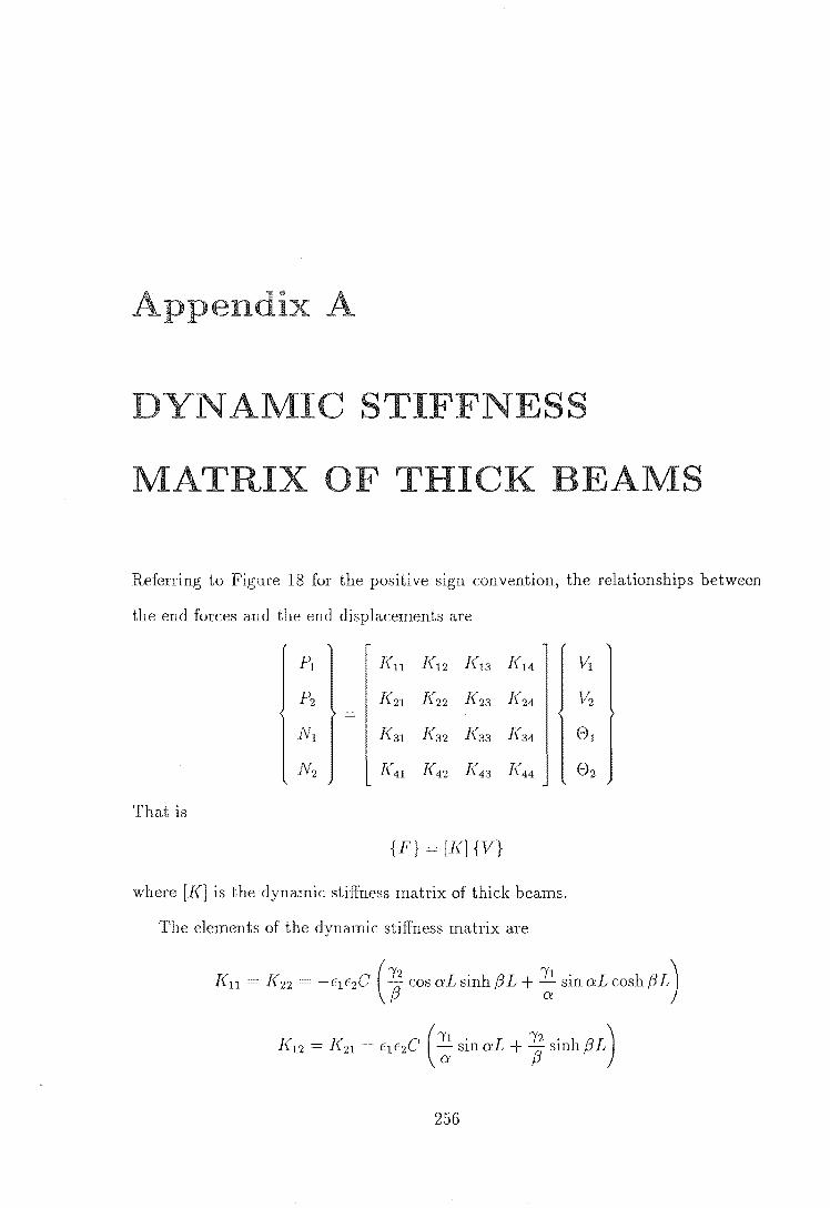
Append3
DYNAMIC S N
MATRI OF MS
Referring to Figure 18 for the positive sign convention, relationships between
the end forces and the end displacements are
PI ](11 ](12 ](13 [(14 Vi
P2 ](21 ](22 ](23 ](24 II;
Nl ](31 ](32 ](33 ](34 8 1
N2 ](41 ](42 ](43 ](44 8 2
That is
{F} = [](] {V}
where [](] is the dynamic stiffness matrix of thick beams.
The elements of the dynamic stiffness matrix are
1(11 K" -E,E,C (; cosaJ,sinhflJ,+ ~ SinaLCOShflL)
](12 = ](21 = E]E2C (: sinaL + ; Sinh,BL)
256

APPENDIX A
where
-](31 = -](13 ](24 = ](42 11/2C { (:~ + ;~) sin aL sinh;3L
+ 12:;3 11 (cos aL cosh ;3 L 1) }
C
-](32 -1(23 = ](14 ](41 = tlt2C (cos aL cosh;3L)
[{33 - ](44 t1 C ( : cos aL sinh;3L ; sin aL cosh;3L )
1(34 = 1{43 tIC (; sinaL - : sinh;3L)
... --2a2 = pw2 (_1_ +~) + Ip 2W 4 (_1 __ ~)2 + 4pAw
2
kG E V kG E EI
2 2( 1 1) 2;3 = -pw - + - + kG E
2 ,1 = a
2 pw2
,2 =;3 + kG
sin aL sinh;3L + 2t2 (cos aL cosh;3L -1)
257

• P IX
QU M T N OR
AMO G EAM
The kinetic energy T of a moving beam is
T - pA c2 + - + c- dx 11L [ (OV Ov) 2] 2 0 ot ox
The potential energy U of a beam under a longitudinal force R is
The tension R is given by
where Eo is the initial tension, and 'fJ is a constant depending on the type of the
straining device. For the counterweight mechanism, 'fJ L
The energy terms can be substituted into the Hamilton's principle
8U) dt = j t2 {L{PA (OV +cOV) (0 (rSv) + cO (rSV)) t1 io ot ox ot Ox
_ E I 02v 02 _ R ov 0 ( 8v )} dx dt ox2 ox2 Ox ox
o.
258

APPENDIX B 259
Integrating the above equation by parts gives
o
Therefore) the equation of motion is
o
and the boundary condi tions are
EPv ) av av v 0 or EI ax3 + ((1- 77) pAc2
Ro ax + pAc at = 0
av a2v ax 0 or EI ax2 = 0