vibration of prestressed membrane structures in air · vibration of prestressed membrane structures...

AIAA 2002-1368Vibration of Prestressed MembraneStructures in AirS. Kukathasan and S. PellegrinoDepartment of Engineering, University of Cambridge,Cambridge CB2 1PZ, UK

43rd AIAA/ASME/ASCE/AHS/ASCStructures, Structural Dynamics, and

Materials Conference22-25 April 2002

Denver, COFor permission to copy or republish, contact the American Institute of Aeronautics and Astronautics1801 Alexander Bell Drive, Suite 500, Reston, VA 20191–4344

AIAA-2002-1368

VIBRATION OF PRESTRESSED MEMBRANE STRUCTURES IN AIR

S. Kukathasan∗ and S. Pellegrino†

Department of Engineering, University of CambridgeTrumpington Street, Cambridge, CB2 1PZ, U.K.

Abstract

Including air effects in the finite-element model of largedeployable membrane structures can lead to consid-erable simplification in the ground testing of thesestructures, by removing the need to carry out exten-sive tests in vacuum chambers. This paper presentsa finite-element modelling technique which simulatesvery accurately the air-membrane interaction. Resultsobtained with the ABAQUS package are comparedwith three test cases, which include a closed-form an-alytical solution and two sets of experiments.

Introduction

Thin membranes are increasingly being considered forlarge deployable space structures applications, due tothe growing requirement for furlable reflecting surfacesfor solar sails, space radars and reflector antennas.These structures are generally very flexible, and thereis a need to have accurate models to predict their vi-bration behavior, which impacts their geometric accu-racy and hence their performance, and may also leadto dynamic coupling with the attitude control systemof the spacecraft.

It is well-known that large lightweight membranestructures vibrating in air have lower natural frequen-cies and higher damping than in vacuum, hence ingeneral ground tests on these structures need to bedone in a vacuum chamber. However, this is expen-sive and far from straightforward. For example, re-cent tests of a large membrane sunshield for the NextGeneration Space Telescope1 posed considerable chal-lenges, due to: (i) size limitations of existing vac-uum chambers, (ii) difficulty of measuring whole modelresponse through the glass portholes of the cham-ber, and (iii) difficulty of operating dynamic shakers,etc. under vacuum. Additional difficulties have beenidentified.2 Therefore, it is of interest to develop pro-cedures whereby at least some experiments are con-

ducted in air and validated against numerical models.Of course, the presence of air around the membraneneeds to be properly included in these models. Oncevalidated in this way, the numerical models could thenbe used to predict the vibration behavior in vacuum.

The vibration of a large membrane structure sur-rounded by an unbounded volume of air is a coupledfluid-structure interaction problem. Because the airdisplacements are small, the air can be treated as anacoustic medium which interacts with the vibratingsurface through the acoustic pressure that it applieson it. Also, since we are only interested in finding theeffects on the structure of the presence of the fluid,effects such as acoustic scattering or radiation in thefluid need not be considered.

The aim of this paper is to present a techniquefor modelling prestressed membrane structures vibrat-ing in air by means of a standard finite element pack-age. The accuracy of the model will be checked againstthree separate test cases, one based on a closed-formanalytical solution and two based on experiments.

The layout of this paper is as follows. First, a briefreview of relevant literature is presented. Second, aclosed-form analytical solution is derived to estimatethe natural frequencies of an infinite flat membranein air. Third, experiments carried out on triangular,prestressed membranes to measure their resonant fre-quencies and corresponding mode shapes in air are pre-sented. Fourth, a finite element modelling technique ispresented and validated against the analytical solutionand experimental results. A discussion concludes thepaper.

Background

Most previous work on the vibration of elastic struc-tures surrounded by a fluid has been focussed onplates; only recently has work specific to membranesbeen published.1−4 However, because the same general

∗Research Student.†Professor of Structural Engineering, Associate Fellow AIAA. [email protected]

Copyright c© 2002 by S. Pellegrino. Published by the American Institute of Aeronautics and Astronautics, Inc. with permission.

1American Institute of Aeronautics and Astronautics

approach can be applied to both types of structures, itis appropriate to begin by reviewing some key resultsfor plates.5

The vibration response of an infinite plate in anunbounded fluid medium changes at the so-called coin-cidence frequency.6 At this transition the fluid loadingeffect on the vibrating plate changes from providinga non-structural mass to providing radiation damp-ing. When the plate vibrates below the coincidencefrequency, it accelerates and compresses a small layerof fluid,5−8 whose thickness decreases as the frequencyincreases. An analytical solution can be obtained6 byassuming that the natural modes of the fluid loadedplate are identical to the modes in vacuum. Plates offinite size are slightly damped by the fluid even be-low the coincidence frequency, as well as showing anadded mass effect.9 This is because edge effects causeacoustic radiation.8

Fluid-structure interaction problems are normallysolved by combining a finite element (FE) model ofthe structure with a model of the fluid, computed us-ing either FE or boundary element (BE) methods. Inthe case of a structure fully submerged in an infinitefluid medium, a FE representation of the fluid requiresa very large mesh. Boundary element methods tend tobe more attractive, as a 3-D infinite medium can bemodelled with 2-D surface elements.10−12 Reference10

gives a thorough explanation of how to find the nat-ural frequency of any structure submerged in an infi-nite air medium using a combined FE/BE model. Italso points out that achieving convergence to the natu-ral frequency can prove troublesome; several iterationsare often required. Two major disadvantages of BEmethods13 are that they remain computationally ex-pensive because of the non-bandedness of the stiffnessmatrix, in spite of the reduction in dimensionality, andalso because the formulation becomes singular at thecoincidence frequency. On the other hand, FE rep-resentations of an infinite fluid medium using a finitedomain with carefully chosen boundaries have beenshown to be possible, without affecting the acousticfield.14−15 Any artificial exterior acoustic boundariesshould be placed above a minimum distance from thevibrating surface. The distance and type of the exte-rior boundaries need to be selected such that they donot interfere with the origin of the acoustic waves.16

Membranes have negligible out-of-plane stiffness,unless they are prestressed. A study of the effects ofprestress and air pressure on the vibration of a trian-gular membrane with edge cords3 determined the nat-ural frequencies and the corresponding mode shapesat different air pressures, i.e. in vacuum, at 0.61 atmand at 1 atm. A physical model was excited by anelectrodynamic shaker attached to a corner of the tri-angle, and the dynamic response was measured using

a non-contact capacitance device. These experimentsindicate significantly lower and more closely spacednatural frequencies at higher air pressures, and alsosome distortion of the mode shapes in vacuum. Theexperimental results presented in this reference are avery valuable benchmark against which to test new so-lutions. FE predictions of the in vacuo mode shapeswere obtained. An approximate analytical method wasalso proposed, which simulates air effects by adding anon structural mass equal to the volume of air con-tained in an envelope defined by the radius of thelargest circle inscribed in the triangle. This methodwas able to predict the accuracy of the fundamentalnatural mode to an accuracy of 10% but was muchless accurate for higher modes. For example, the sixthnatural frequency in air was underestimated by 27%and the corresponding mode shape was also poorly es-timated.

The lack of agreement between the experimentalresults and the approximate method in Ref. 3 is mainlydue to the assumption of the same air mass for eachmode. In reality, the air mass participating in themembrane vibration decreases with the increase ofmode number6. This points to the need for a propercriterion for estimating the added mass. Several at-tempts at refining Ref. 3 were made at the early stagesof the present study17 but, although some improve-ments were indeed achieved, it was concluded that sim-ple geometric criteria cannot provide high accuracy.

An Analytical Solution

The scope for analytical solutions is very limited,hence we turn to the standard solution for an infiniteflat plate surrounded by a fluid8 which can be adaptedto infinite membranes, as shown next. It is assumedthat the in vacuo modes are preserved in air. The cou-pling is achieved by assuming the same wavelength forthe membrane and the air, and by matching the trans-verse response of the membrane to the air pressure atthe interface.

Membrane Vibration in Vacuum

Consider a thin, flat membrane in an x, y coordinatesystem. It is subject to biaxial tension T per unitlength, which will be assumed to remain constant whenthe membrane vibrates, and mass per unit area ms.

Denoting by w(x, y, t) the out-of-plane displace-ment of point (x, y) at time t and neglecting the bend-ing stiffness of the membrane, the differential equation


of motion has the form18

T

(∂2w

∂x2 +∂2w

∂y2

)= ms

∂2w

∂t2(1)

If the membrane is either infinitely long in both x andy, or of finite dimensions but of rectangular shape, thegeneral steady-state solution of Equation (1) is of theform

w = w̃eiωte−i(ksxx+ksyy) (2)

where w̃ is the displacement amplitude, ksx and ksy

are the elastic wave number components along the xand y directions —of dimension (length−1)—, and ωis the particular frequency of interest. Note that thesubscript s stands for structure.

These wave number components are related to thecorresponding wave lengths, λsx and λsy, of the vibra-tion mode shape in the x and y directions by

ksx =2πλsx

, ksy =2πλsy

(3)

Substituting Equation (2) into (1), we obtain

ksx2 + ksy

2 =msω

2

T(4)

and defining the elastic wave number, ks, of the mem-brane at frequency ω

k2s = k2

sx + k2sy (5)

we obtain

ω = ks

√T

ms(6)

Note that this corresponds to a one-dimensionalwave in a particular direction ξ, defined by the vectorsum of λsx and λsy, with wave length λs = 2π/ks.

Pressure Waves in Air

Steady-state pressure waves in one or more dimen-sions, in a medium of density ρ and bulk modulus Bsatisfy the Helmholtz equation.7 We are particularlyinterested in two-dimensional waves, hence

(∇2 + ka2)p = 0 (7)

where p = p(ξ, η) is the pressure at point (ξ, η), vary-ing with time at frequency ω, and ka is the acousticwave number

ka = ω

√ρ

B(8)

The general solution of Equation (7) is a harmonicfunction of horizontal distance, ξ, and vertical dis-tance, η, with acoustic wave numbers kaξ and kaη inthe two directions, hence

p = p̃eiωte−i(kaξξ+kaηη) (9)

Substituting Equation (9) into (7) leads to a relation-ship between the acoustic wave numbers that is anal-ogous to Equation (5)

ka2 = kaξ

2 + kaη2 (10)

Coupled Vibration

The response of a membrane with air on one side onlycan be analysed as follows. The two solutions pre-sented above, which are valid for any frequency ω, arecoupled by imposing that the acoustic wave compo-nent along the ξ-direction matches the structural wavealong the ξ-direction. Therefore, the correspondingwave numbers must also match, hence

ks = kaξ (11)

It follows that from now on the η-direction will beperpendicular to the membrane and the correspondingwave number is then obtained by substituting Equa-tion (11) into Equation (10). Noting that for thinmembranes in air the elastic wave number ks is higherthan the acoustic wave number ka gives

kaη = −i

√ks

2 − ka2 (12)

In the presence of air, Equation (1) becomes

T

(∂2w

∂x2 +∂2w

∂y2

)− p = ms

∂2w

∂t2(13)

where it can be shown7 that the pressure p on themembrane is coupled to the motion of the membranethrough

∂p

∂η= −ρ

∂2w

∂t2at η = 0 (14)

Differentiation of Equation (9) with respect to η yields,after substituting Equation (9)

∂p

∂η= −ikaηp (15)

Then, substitution into Equation (14) gives

p =ρ

ikaη

∂2w

∂t2(16)


Substituting Equation (16) into Equation (13),

T

(∂2w

∂x2 +∂2w

∂y2

)− ρ

ikaη

∂2w

∂t2= ms

∂2w

∂t2(17)

Substituting Equation (12) for kaη and re-arranging

T

(∂2w

∂x2 +∂2w

∂y2

)=

(ms +

ρ√k2

s − k2a

)∂2w

∂t2(18)

Thus, comparing Equation (18) with Equation (1) itcan be seen that the presence of air introduces an addi-tional air mass ma into the equation of motion, where

ma =ρ√

k2s − k2

a

, if ks > ka (19)

This amounts to saying that a layer of air of thick-ness 1/

√k2

s − k2a vibrates together with the mem-

brane. If ks < ka the added air mass is imaginary,which means that air adds to the damping of the sys-tem. It is noted that when the frequency of vibrationincreases, then ks and ka increase proportionally, thusthe air mass ma decreases.

In conclusion, an infinite membrane of mass ms

per unit area which is subject to biaxial tension T hasinfinitely many sinusoidal vibration modes. For anychosen mode, of wave lengths λsx and λsy, we can cal-culate the wave number from Equations (5, 3)

ks = 2π

√1

λ2sx

+1

λ2sy

(20)

and the corresponding natural frequency of vibrationin vacuum from Equation (6)

ωvacuum = ks

√T

ms(21)

The ratio of the wave numbers can be written, fromEquations (6, 8), as

ks

ka=

√ms

T

B

ρ(22)

It is noted that this ratio is not a function of the fre-quency of vibration. Therefore, the type of fluid load-ing effect on the membrane does not change with thefrequency of vibration. Hence, the nature of fluid load-ing on the membrane depends only on its mass per unitarea and the prestress.

If the membrane vibrates in air, its mode shapesdo not change but the natural frequency of vibrationbecomes

ωair = ks

√T

ms + ma(23)

where the air mass is iteratively calculated from

ma =ρ√

k2s − ω2

airρ/B(24)

If there is air on both sides of the membrane, the sameanalysis can be repeated to obtain an equation like(24), but with a factor of 2 at numerator.

An Experiment

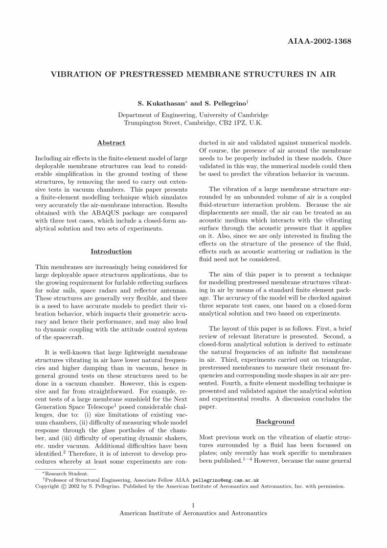
The natural frequencies and mode shapes of a triangu-lar membrane vibrating in air were measured. A pho-tograph of the experimental model is shown in Figure 1and its dimensions are defined in Figure 2.

A triangular steel framework, rigidly fixed to theground, was used to provide a rigid support for themembrane structure. The membrane itself is madeof 0.05 mm thick aluminized Mylar foil, and has theshape of a right angle triangle with curved edges withsag-to-depth ratio is 20. A sleeve is formed along eachedge of the foil, with Kapton tape, and Kevlar cordswith a diameter of 0.92 mm are located inside thesleeve. Further details on the materials used are givenin Table 1.

Figure 1: Experimental model.

Table 1: Material properties of experimental model.

Membrane Cord ConnectorMaterial Mylar Kevlar Al-alloyDensity (kg/m3) 1070 1450 2700E (kN/mm2) 3.5 131 70ν 0.35 0.30 0.33Mass (g) 5.1 1.3 12.2

The two cords that meet at each corner of the trian-gle are joined together with a steel loop (but a largerconnector is used near the 90 deg corner) and gluedwith epoxy; then they are taken together to a bracket


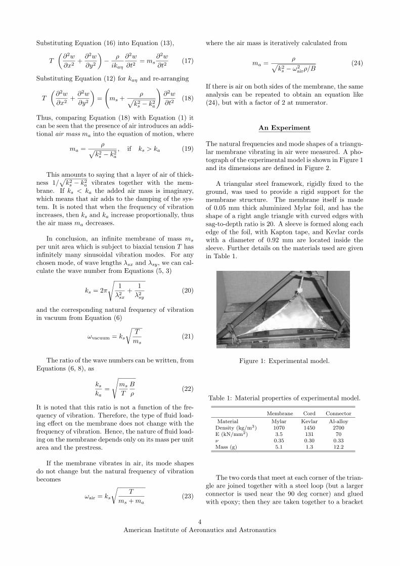
attached to the steel frame. Thus, in effect the mem-brane is connected to the frame by three cables, whosedirections meet at a point, thus satisfying equilibrium.One of the three cables is connected to a strain-gaugedturnbuckle; the shape of the triangle and the directionsof the cables are such that the membrane is in uniformbi-axial prestress. All experiments reported in this pa-per were conducted at a uniform prestress of 20 N/min the membrane.

Membrane

400 mm

500 mm

300 mm

Connector

Strain gaugedturnbuckle

Figure 2: Schematic diagram of experimental model.

Modal identification tests were carried out, by hit-ting the surface of the connector with a PCB O86D80impulse hammer fitted with a piezoelectric head,19 andby measuring the response of the membrane at 50points with a Polytec PSV300 scanning laser vibrom-eter. Non-reflective powder had to be sprayed on themembrane surface, to avoid the laser beam from beingdeflected entirely away from the laser head. To reducenoise, each measurement was repeated five times andthe results were averaged. After measuring all the tar-get points, the Fast Fourier Transform (FFT) of theabove signals was computed in order to obtain the fre-quency response function and the mode shapes of themodel.

Finite Element Modelling

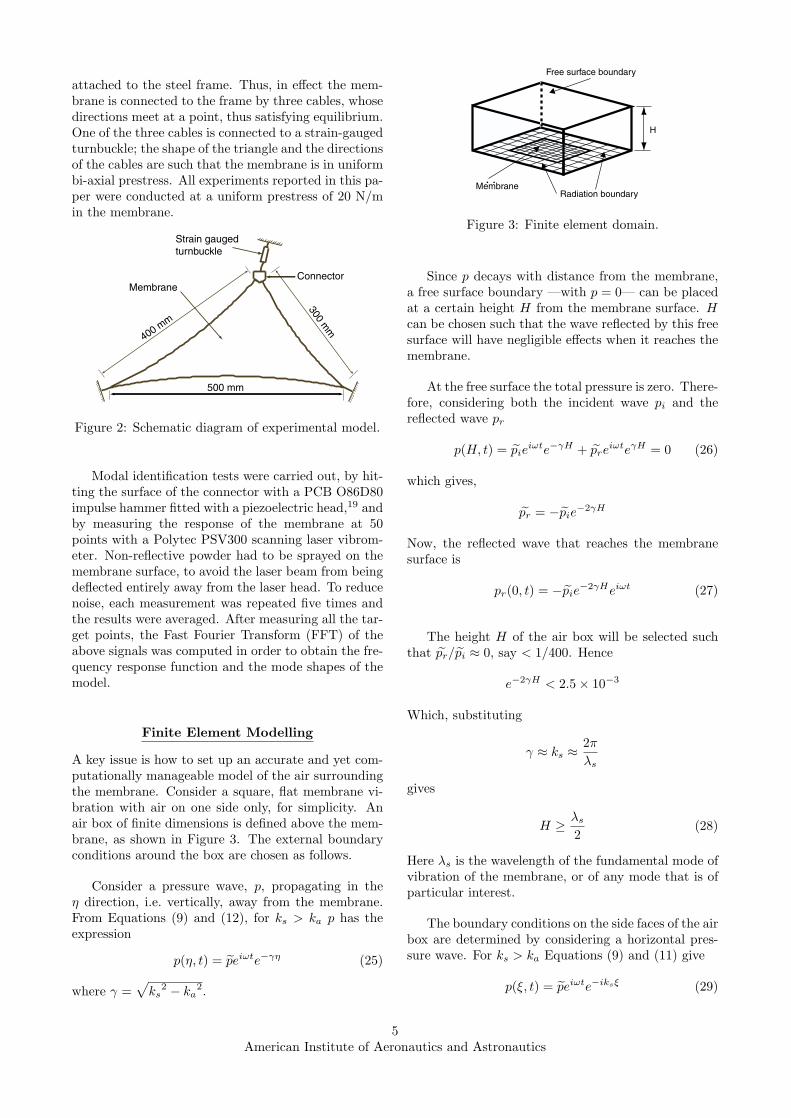
A key issue is how to set up an accurate and yet com-putationally manageable model of the air surroundingthe membrane. Consider a square, flat membrane vi-bration with air on one side only, for simplicity. Anair box of finite dimensions is defined above the mem-brane, as shown in Figure 3. The external boundaryconditions around the box are chosen as follows.

Consider a pressure wave, p, propagating in theη direction, i.e. vertically, away from the membrane.From Equations (9) and (12), for ks > ka p has theexpression

p(η, t) = p̃eiωte−γη (25)

where γ =√

ks2 − ka

2.

Free surface boundary

Radiation boundaryMembrane

H

Figure 3: Finite element domain.

Since p decays with distance from the membrane,a free surface boundary —with p = 0— can be placedat a certain height H from the membrane surface. Hcan be chosen such that the wave reflected by this freesurface will have negligible effects when it reaches themembrane.

At the free surface the total pressure is zero. There-fore, considering both the incident wave pi and thereflected wave pr

p(H, t) = p̃ieiωte−γH + p̃re

iωteγH = 0 (26)

which gives,

p̃r = −p̃ie−2γH

Now, the reflected wave that reaches the membranesurface is

pr(0, t) = −p̃ie−2γHeiωt (27)

The height H of the air box will be selected suchthat p̃r/p̃i ≈ 0, say < 1/400. Hence

e−2γH < 2.5 × 10−3

Which, substituting

γ ≈ ks ≈ 2πλs

gives

H ≥ λs

2(28)

Here λs is the wavelength of the fundamental mode ofvibration of the membrane, or of any mode that is ofparticular interest.

The boundary conditions on the side faces of the airbox are determined by considering a horizontal pres-sure wave. For ks > ka Equations (9) and (11) give

p(ξ, t) = p̃eiωte−iksξ (29)


which shows that p propagates without decaying.Therefore, the type of boundary condition that mini-mizes any interference is a radiation boundary. It hasbeen found that boundaries of this type, placed on thesides of the air box, do not affect the frequency of themembrane if they are at a distance of no less than λs/2from the edges of the membrane.

Choice of Elements

The ABAQUS FE package20 was used throughoutthis study; here we give some details on the choiceof elements. The membrane was modelled using 9-node second-order quadrilateral membrane elements(M3D9) and the air domain with 3D solid acous-tic elements, either 20-node second-order brick acous-tic elements (AC3D20) or 15-node triangular prisms(AC3D15). These elements use acoustic pressure asa variable. The coupling between acoustic and mem-brane elements was set up by defining two surfacesalong the interface, i.e. one lying on top of the mem-brane and the other at the bottom of the acoustic el-ements, and by tying together the nodes in the twosurfaces (*TIE). An advantage of defining these sur-faces is that the two element meshes do not need tohave matching densities. The acoustic surface had tobe defined as the “master” surface, because the modelof the membrane was more refined. The horizontalsurface around the membrane was modelled as a “rigidwall”, which is the default boundary condition appliedby ABAQUS.

Analysis Details

A complete analysis consists of two main steps. First,a static analysis in which the geometric stiffness of themembrane, without air, resulting from the prestress iscalculated. Second, a dynamic analysis of the coupledair-membrane model which estimates the resonant fre-quencies and corresponding mode shapes.

Prestress of the membrane and any cords is de-fined as an initial stress (*INITIAL CONDITIONS,TYPE=STRESS). It is best to begin the analysis withan equilibrium iteration; if the given prestress distri-bution is not in equilibrium, ABAQUS will find one,but it is important to check that the prestress levelhas not significantly decreased. Once the prestress isknown in full, a geometrically non-linear static anal-ysis is carried out (*STEP, NLGEOM), in which thegeometric stiffness matrix is calculated. This geomet-ric stiffness is automatically included in the followingdynamic analysis.

The FE model of a coupled air-membrane problemhas unsymmetric overall stiffness and mass matrices,

although the eigenvalues are real.15 Therefore a com-plex eigensolver is needed, but this is not available inABAQUS.20 A way around is to use a frequency re-sponse analysis instead (*STEP, *STEADY STATEDYNAMICS, DIRECT), by applying a unit, steady-state input load at a chosen node of the membraneand by varying the frequency over the range of inter-est. The responses of all membrane nodes to this inputare recorded over the whole range of frequencies. Theresponse amplitudes at a chosen node are plotted as afunction of frequency and the peaks in this plot iden-tify the resonant frequencies. The corresponding modeshapes are obtained from the real part of the responseof each node. Because damping is small, out-of-phaseeffects are neglected.

Although computationally more expensive thanmode-based steady-state dynamic analysis, thismethod is more accurate. A further advantage is thatproportional material damping can be easily incorpo-rated as complex mass and stiffness matrices are noproblem.

Three Test Cases

Comparison with Analytical Solution

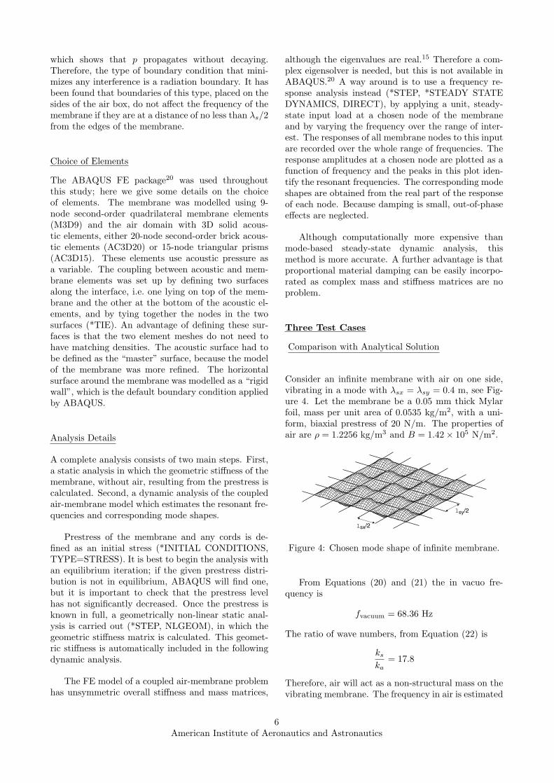
Consider an infinite membrane with air on one side,vibrating in a mode with λsx = λsy = 0.4 m, see Fig-ure 4. Let the membrane be a 0.05 mm thick Mylarfoil, mass per unit area of 0.0535 kg/m2, with a uni-form, biaxial prestress of 20 N/m. The properties ofair are ρ = 1.2256 kg/m3 and B = 1.42 × 105 N/m2.

lsy/2

lsx/2

Figure 4: Chosen mode shape of infinite membrane.

From Equations (20) and (21) the in vacuo fre-quency is

fvacuum = 68.36 Hz

The ratio of wave numbers, from Equation (22) is

ks

ka= 17.8

Therefore, air will act as a non-structural mass on thevibrating membrane. The frequency in air is estimated


iteratively from Equations (23) and (24), as

fair = 47.95 Hz

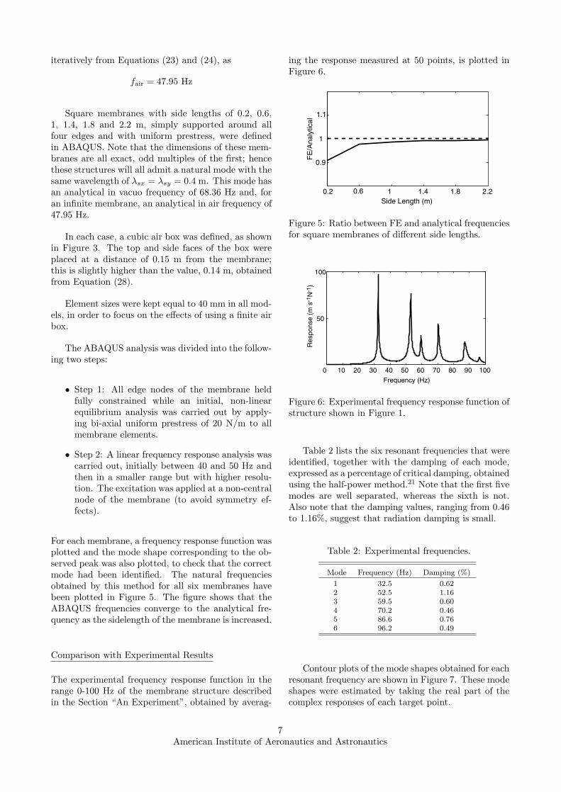
Square membranes with side lengths of 0.2, 0.6,1, 1.4, 1.8 and 2.2 m, simply supported around allfour edges and with uniform prestress, were definedin ABAQUS. Note that the dimensions of these mem-branes are all exact, odd multiples of the first; hencethese structures will all admit a natural mode with thesame wavelength of λsx = λsy = 0.4 m. This mode hasan analytical in vacuo frequency of 68.36 Hz and, foran infinite membrane, an analytical in air frequency of47.95 Hz.

In each case, a cubic air box was defined, as shownin Figure 3. The top and side faces of the box wereplaced at a distance of 0.15 m from the membrane;this is slightly higher than the value, 0.14 m, obtainedfrom Equation (28).

Element sizes were kept equal to 40 mm in all mod-els, in order to focus on the effects of using a finite airbox.

The ABAQUS analysis was divided into the follow-ing two steps:

• Step 1: All edge nodes of the membrane heldfully constrained while an initial, non-linearequilibrium analysis was carried out by apply-ing bi-axial uniform prestress of 20 N/m to allmembrane elements.

• Step 2: A linear frequency response analysis wascarried out, initially between 40 and 50 Hz andthen in a smaller range but with higher resolu-tion. The excitation was applied at a non-centralnode of the membrane (to avoid symmetry ef-fects).

For each membrane, a frequency response function wasplotted and the mode shape corresponding to the ob-served peak was also plotted, to check that the correctmode had been identified. The natural frequenciesobtained by this method for all six membranes havebeen plotted in Figure 5. The figure shows that theABAQUS frequencies converge to the analytical fre-quency as the sidelength of the membrane is increased.

Comparison with Experimental Results

The experimental frequency response function in therange 0-100 Hz of the membrane structure describedin the Section “An Experiment”, obtained by averag-

ing the response measured at 50 points, is plotted inFigure 6.

0.2 0.6 1 1.4 1.8 2.2

0.9

1

1.1

Side Length (m)

FE

/Ana

lytic

al

Figure 5: Ratio between FE and analytical frequenciesfor square membranes of different side lengths.

0 10 20 30 40 50 60 70 80 90 100

50

100

Frequency (Hz)

Res

pons

e (m

s-1

N-1

)

Figure 6: Experimental frequency response function ofstructure shown in Figure 1.

Table 2 lists the six resonant frequencies that wereidentified, together with the damping of each mode,expressed as a percentage of critical damping, obtainedusing the half-power method.21 Note that the first fivemodes are well separated, whereas the sixth is not.Also note that the damping values, ranging from 0.46to 1.16%, suggest that radiation damping is small.

Table 2: Experimental frequencies.

Mode Frequency (Hz) Damping (%)1 32.5 0.622 52.5 1.163 59.5 0.604 70.2 0.465 86.6 0.766 96.2 0.49

Contour plots of the mode shapes obtained for eachresonant frequency are shown in Figure 7. These modeshapes were estimated by taking the real part of thecomplex responses of each target point.


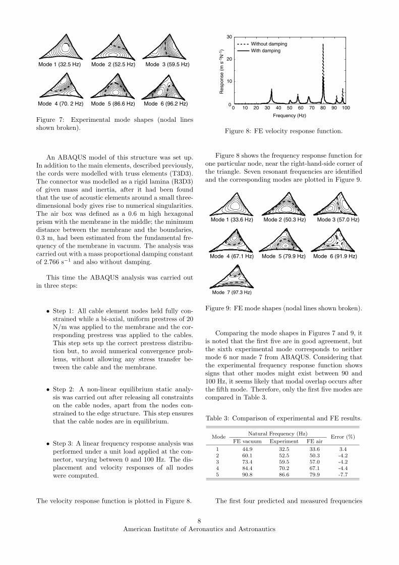
Mode 1 (32.5 Hz) Mode 2 (52.5 Hz) Mode 3 (59.5 Hz)

Mode 4 (70. 2 Hz) Mode 5 (86.6 Hz) Mode 6 (96.2 Hz)

Figure 7: Experimental mode shapes (nodal linesshown broken).

An ABAQUS model of this structure was set up.In addition to the main elements, described previously,the cords were modelled with truss elements (T3D3).The connector was modelled as a rigid lamina (R3D3)of given mass and inertia, after it had been foundthat the use of acoustic elements around a small three-dimensional body gives rise to numerical singularities.The air box was defined as a 0.6 m high hexagonalprism with the membrane in the middle; the minimumdistance between the membrane and the boundaries,0.3 m, had been estimated from the fundamental fre-quency of the membrane in vacuum. The analysis wascarried out with a mass proportional damping constantof 2.766 s−1 and also without damping.

This time the ABAQUS analysis was carried outin three steps:

• Step 1: All cable element nodes held fully con-strained while a bi-axial, uniform prestress of 20N/m was applied to the membrane and the cor-responding prestress was applied to the cables.This step sets up the correct prestress distribu-tion but, to avoid numerical convergence prob-lems, without allowing any stress transfer be-tween the cable and the membrane.

• Step 2: A non-linear equilibrium static analy-sis was carried out after releasing all constraintson the cable nodes, apart from the nodes con-strained to the edge structure. This step ensuresthat the cable nodes are in equilibrium.

• Step 3: A linear frequency response analysis wasperformed under a unit load applied at the con-nector, varying between 0 and 100 Hz. The dis-placement and velocity responses of all nodeswere computed.

The velocity response function is plotted in Figure 8.

0 10 20 30 40 50 60 70 80 90 1000

10

20

30

Frequency (Hz)

Without damping With damping

Res

pons

e (m

s-1

N-1

)

Figure 8: FE velocity response function.

Figure 8 shows the frequency response function forone particular node, near the right-hand-side corner ofthe triangle. Seven resonant frequencies are identifiedand the corresponding modes are plotted in Figure 9.



Mode 7 (97.3 Hz)

Figure 9: FE mode shapes (nodal lines shown broken).

Comparing the mode shapes in Figures 7 and 9, itis noted that the first five are in good agreement, butthe sixth experimental mode corresponds to neithermode 6 nor made 7 from ABAQUS. Considering thatthe experimental frequency response function showssigns that other modes might exist between 90 and100 Hz, it seems likely that modal overlap occurs afterthe fifth mode. Therefore, only the first five modes arecompared in Table 3.

Table 3: Comparison of experimental and FE results.

Mode Natural Frequency (Hz) Error (%)FE vacuum Experiment FE air

1 44.9 32.5 33.6 3.42 60.1 52.5 50.3 -4.23 73.4 59.5 57.0 -4.24 84.4 70.2 67.1 -4.45 90.8 86.6 79.9 -7.7

The first four predicted and measured frequencies


differ by around 4% and the fifth by 7.7 %. Note thatthe difference between frequencies in air and in vac-uum is highest —12.4 Hz, corresponding to a decreaseof 26%— for the fundamental mode and decreases withthe mode number.

Comparison with Sewall’s Experiment

The third test case was based on one of the tests re-ported in Ref. 3. A schematic diagram of the modelstructure is shown in Figure 10, and the experimentalmode shapes are shown in Figure 11.

1.41 m radius

pulley

.0127 mm thick Mylar

1.6 mm diam.steel cable

.9144 m

Figure 10: Membrane tested in Ref. 3.

16.31 Hz 30.95 Hz 32.50 Hz

37.05 Hz

84.08 Hz80.51 Hz

52.77 Hz47.84 Hz

Node

Node

Node

Figure 11: Experimental mode shapes at 93.4 N apextension in air at 0.61 atm (from Ref. 3).

This structure was analysed with ABAQUS. Themembrane and cables were modelled as described pre-viously; the effect of the shaker was modelled as a pointmass. A hexagonal air box, placed at 0.8 m from themembrane, was defined as discussed in the previous

section.

The ABAQUS analysis had three steps, as forthe previous test case, and the measured materialdamping3 was included as a mass proportional damp-ing constant of 1.704 s−1. The frequency responsefunction showed 12 modes between 0 and 100 Hz. Thenodal lines of the corresponding 12 mode shapes areplotted in Figure 12.





Figure 12: FE mode shapes.

Comparing Figure 12 with Figure 11, the secondexperimental mode shape is missing. The reason isthat this mode is anti-symmetric, and hence it is notexcited by symmetric input applied to the ABAQUSmodel. The 2nd, 3rd, 4th and 5th modes from the fi-nite element simulation are in fair agreement with the3rd, 4th, 5th and 6th modes from the experiment, re-spectively. The differences in frequency are very small,from 0.5 to 4%, see Table 4.

Table 4: Comparison of experimental and FE results.

Mode Natural Frequency (Hz) Error (%)Experiment FE air

1 16.3 16.1 1.22 30.9 — —3 32.5 31.5 3.14 37.1 36.9 0.55 47.8 49.7 -4.06 52.8 51.7 2.1

Discussion

The analytical solution for the natural frequenciesof infinite flat membranes vibrating in air has provided


a good insight. When the structural wave number, ks,is greater than the acoustic wave number, ka, whichis the typical case for thin membranes in air, it hasbeen shown that a layer of air moves together withthe vibrating membrane; this air thickness decreaseswith the increase in frequency of vibration. There-fore, the natural frequencies of the membrane in airare lower than its in vacuo frequencies because air actsas a non-structural mass, which is added to the massof the membrane. In the three test cases presented inthis paper the maximum difference was a decrease of29% for one of the fundamental modes, but the highermodes show smaller differences.

Unlike thin plates vibrating in air, thin prestressedmembranes do not show a coincidence frequency, be-cause the ratio between structural and acoustic wavenumbers is not a function of the frequency of vibrationbut only of the prestress and mass per unit area of themembrane.

In the experiment presented as our second test casewe also had ks >> ka and hence air acts mainly (butnot only, due to edge effects) as an added mass. Thisis confirmed by the low damping that has been mea-sured, between 0.4 and 1.2 % of critical.

With this background, we have developed a FEmodelling technique in which the membrane is en-closed in an air box of finite dimensions; these dimen-sions are related to the structural wavelength, λs. Thismodelling technique is reasonably economical of com-puter resources and has been shown to be very accu-rate by comparison with an analytical test case andtwo sets of experimental results. The first test hasshown that the FE model converges to the analyticalsolution for an infinite membrane when the modelledsize of the membrane is increased. The FE solution iswithin 2% of the analytical solution when a membranesize of 1.5 times the structural wavelength or greater ismodelled. The second and third test cases, involvingmembrane structures that are representative of pro-posed applications, have shown that the frequenciesobtained from the FE simulation are typically within4% of the measured frequencies for our own experi-mental results, and within 2% of the published results.Considering that the physical model used for our ex-periments was about one-third the size of that used inRef. 3, it seems reasonable to conclude that the higherlevel of error in the second test case is due to experi-mental error.

Conclusion

The FE simulation technique presented in this paperpredicts the natural frequencies and mode shapes ofmembrane structures vibrating in air with great ac-

curacy. Hence, it is concluded that for model identi-fication purposes it should be possible to reduce theamount of testing that needs to be carried out undervacuum.

Acknowledgments

We thank Dr W.R. Graham for helpful discussions ofair-structure effects and Professor J. Woodhouse forhelp with the experiments.

References

1 Lienard, S., Johnston, J.D., Ross B.P., and Smith,J., “Dynamic testing of a subscale sunshield forthe Next Generation Space Telescope”, Proc. 42ndAIAA/ASME/ASCE/AHS/ASC Structures, Struc-tural Dynamics, and Materials Conference and Ex-hibit, Seattle, WA, 2001, AIAA-2001-1268.2 Pappa, R.S., Lassiter, J.O., and Ross, B.P.,“Structural dynamic experimental activities in ultra-lightweight and inflatable space structures”, Proc.42nd AIAA/ASME/ASCE/AHS/ASC Structures,Structural Dynamics, and Materials Conference andExhibit, Seattle, WA, 2001, AIAA-2001-1263.3 Sewall, J.L., Miserentino, R. and Pappa, R.S., “Vi-bration studies of a lightweight three-sided membranesuitable for space application”, NASA TP 2095, 1983.4 Johnston, J.D., and Lienard, S., “Modellingand analysis of structural dynamics for a one-tenth scale model NGST sunshield”‘ Proc. 42ndAIAA/ASME/ASCE/AHS/ASC Structures, Struc-tural Dynamics, and Materials Conference and Ex-hibit, Seattle, WA, 2001, AIAA-2001-1407.5 Junger, M.C., “Acoustic Fluid-elastic structure in-teractions: basic concepts”, Computers and Struc-tures, Vol. 65, No. 3, 1997, pp. 287-293.6 Junger, M.C., “Normal modes of submerged platesand shells”, Symposium on Fluid-Solid Interaction,ASME, 1967, pp. 79-119.7 Junger, M.C., and Feit, D., Sound, Structures, andTheir Interaction, MIT Press, Massachusetts, 1986.8 Fahy, F.J., Sound and Structural Vibration: Radi-ation, Transmission and Response, Academic PressLtd., 1985.9 Davies, H.G., “Low frequency random excitation ofwater-loaded rectangular plates”, Journal of Soundand Vibration Vol. 15, No. 1, 1971, pp. 107-126.10 Sygulski, R. “Dynamic analysis of open membranestructures interacting with air”, International Journalfor Numerical Methods in Engineering, Vol. 37, 1994,pp. 1807-1823.11 Zienkiewicz, O.C., Kelly, D.W., and Bettess, P.“The coupling of the finite element method and bound-ary solution procedures”, International Journal for


Numerical Methods in Engineering, Vol. 11, 1977, pp.355-375.12 Everstine, G.C., and Henderson, F. M., “Coupledfinite element/boundary element approach for fluid-structure interaction”, Journal of Acoustical Societyof America, Vol. 87, No. 5, 1989, pp. 1938-1947.13 Pinsky, P.M. and Abbound, N. N., “Two mixedvariational principles for exterior fluid-structure inter-action problems”, Computers and Structures, Vol. 33,No. 3, 1989, pp. 621-635.14 Zienkiewicz, O.C., and Newton, R.E., “Coupledvibrations of a structure submerged in a compressiblefluid”, Proc. Sym. Finite Element Techniques, 1969,pp. 359-379.15 Everstine, G.C., “Finite element formulations ofstructural acoustics problems”, Computers and Struc-tures, Vol. 65, No. 3, 1997, pp. 307-321.16 Zienkiewicz, O.C. and Bettess, P., “Fluid-structure

dynamic interaction and wave forces: an introductionto numerical treatment”, International Journal forNumerical Methods in Engineering, Vol. 13, 1978, pp.1-16.17 Kukathasan, S. Vibration of prestressed membranestructures, M.Phil. Dissertation, University of Cam-bridge, 2000.18 Rayleigh, J.W.S. The Theory of Sound, Vol. 2,Dover, New York, 1945.19 Ewins, D.J., Modal Testing: Theory, Practice andApplication, Research Studies Press Ltd., England,2000.20 Hibbitt, Karlsson and Sorensen Inc., ABAQUSStandard User’s Manuals, Version 6.2, Pawtucket, RI,USA, 2001.21 Meirovitch, L., Elements of Vibration Analysis,McGraw-Hill Inc., 1986.


vibration of prestressed membrane structures in air · vibration of prestressed membrane structures...

Documents