vibro-acoustical consideration emfi-actuator

V T T P U B L I C A T I O N S

TECHNICAL RESEARCH CENTRE OF FINLAND ESPOO 1999

Ari Saarinen

EMFi-actuator:vibro-acoustical consideration

4 0 5

VT

T P

UB

LICA

TIO

NS

405E

MF

i-actuator: vibro-acoustical considerationA

ri Saarinen

Tätä julkaisua myy Denna publikation säljs av This publication is available from

VTT TIETOPALVELU VTT INFORMATIONSTJÄNST VTT INFORMATION SERVICEPL 2000 PB 2000 P.O.Box 2000

02044 VTT 02044 VTT FIN–02044 VTT, FinlandPuh. (09) 456 4404 Tel. (09) 456 4404 Phone internat. + 358 9 456 4404Faksi (09) 456 4374 Fax (09) 456 4374 Fax + 358 9 456 4374

ElectroMechanical Film (EMFi) is an acoustic actuator and sensor material.An application area where the EMFi-actuator appears very promising is activenoise control (ANC). In this paper the vibro-acoustical properties of theEMFi-actuator are studied. The examination is carried out by modelling theoperation of the actuator and by comparing the modelling results to thecorresponding measured values. Means to increase the radiated sound powerof the actuator element without increasing concurrently the distortion of theradiator are presented. Also the potentiality to evaluate the A-weightedstandard deviation of the sound power of the equipment to be measured fromthe measurement results without specifying the type of emitted sound radiatedby the equipment is presented.

ISBN 951–38–5554–6 (soft back ed.) ISBN 951–38–5555–4 (URL: http://www.inf.vtt.fi/pdf/)ISSN 1235–0621 (soft back ed.) ISSN 1455–0849 (URL: http://www.inf.vtt.fi/pdf/)

VTT PUBLICATIONS 405

TECHNICAL RESEARCH CENTRE OF FINLANDESPOO 1999

EMFi-actuator:vibro-acoustical consideration

Ari SaarinenVTT Building Technology

ISBN 951–38–5554–6 (soft back ed.)ISSN 1235–0621 (soft back ed.)

ISBN 951–38–5555–4 (URL: http://www.inf.vtt.fi/pdf/)ISSN 1455–0849 (URL: http://www.inf.vtt.fi/pdf/)

Copyright © Valtion teknillinen tutkimuskeskus (VTT) 1999

JULKAISIJA – UTGIVARE – PUBLISHER

Valtion teknillinen tutkimuskeskus (VTT), Vuorimiehentie 5, PL 2000, 02044 VTTpuh. vaihde (09) 4561, faksi (09) 456 4374

Statens tekniska forskningscentral (VTT), Bergsmansvägen 5, PB 2000, 02044 VTTtel. växel (09) 4561, fax (09) 456 4374

Technical Research Centre of Finland (VTT), Vuorimiehentie 5, P.O.Box 2000, FIN–02044 VTT, Finlandphone internat. + 358 9 4561, fax + 358 9 456 4374

VTT Rakennustekniikka, Rakennusfysiikka, talo- ja palotekniikka, Lämpömiehenkuja 3, PL 1804, 02044 VTTpuh. vaihde (09) 4561, faksi (09) 455 2408

VTT Byggnadsteknik, Byggnadsfysik, hus- och brandteknik, Värmemansgränden 3, PB 1804, 02044 VTTtel. växel (09) 4561, fax (09) 455 2408

VTT Building Technology, Building Physics, Building Services and Fire Technology,Lämpömiehenkuja 3, P.O.Box 1804, FIN–02044 VTT, Finlandphone internat. + 358 9 4561, fax + 358 9 455 2408

Technical editing Kerttu Tirronen

Libella Painopalvelu Oy, Espoo 1999

3

Saarinen, Ari. EMFi-actuator: vibro-acoustical consideration. Espoo 1999. Technical ResearchCentre of Finland, VTT Publications 405. 109 p. + app. 30 p.

Keywords EMFi-actuator, actuators, vibration, acoustic properties, modelling, evaluation,vibro-acoustical properties, sound production, measurement

AbstractIn this paper, the vibro-acoustical properties of the EMFi-actuator are studied.The examination is carried out by modelling the operation of the actuator and bycomparing the modelling results to the corresponding measured values in casethey are available. The modelling is based on an analytical approach. Theequations used are derived in the Appendices. Consideration on the properties ofthe vibration is divided into three parts: the basic vibration of the film, vibrationof the film in the time domain and vibration of the functional elements of theactuator. The sound production properties of the actuator have been examined inthe free acoustic field and in cases with boundaries near the source. The effect ofthe different vibration distributions of the actuator film and impedance loadingon the emitted sound has been studied. Also the radiation pattern of the actuatoris modelled and compared to the measured results.

The general vibro-acoustical functioning of the EMFi-actuator is stated in theimpedance-oriented form by evaluating the loading impedance of the vibratingfilm based on its boundary conditions. The basic vibration functioning of theactuator film in the frequency domain is predicted by using a linear second-orderordinary differential equation with constant coefficients. In the time domain thenon-linear effects of the spring force and electric forces acting on the actuatorfilm are considered. The recoil effect of the actuator is studied with a normal-mode method of dynamic analysis. It is found that the response of the supportingstructure may decrease about a decade without influencing the response of theactuator film.

The use of the arithmetic average value of the vibration deflection of the EMFi-actuator in the prediction of sound power or sound pressure in the acoustic farfield at low frequencies is compared to the frequency or spatially dependent

4

vibration of the actuator film. The value of the arithmetic average of vibration isvalid even when the outward impedance of the film is not taken intoconsideration. The large dipole type actuators are more effective sound radiatorsthan monopole sources. The effect of the thickness of the absorbent materialunder the dipole actuator, the radiation pattern and the effect of the boundaryconditions of the vibrating cell on the radiating sound power are considered. Themeasured and predicted values of radiation patterns are very similar in everyangle. The rigidly supported boundary of the actuator cell enables the actuatorpanel to radiate much more sound power with all the different even modes thanit is possible with a simply supported boundary condition. The basic problemsconcerning the operation of an EMFi-actuator are related to its ineffective lowfrequency sound production and the distortion caused by non-linear vibration. Itis possible to increase the sound power radiation properties of the monopole ordipole type functional modes of the actuator by making the deflection of themembrane larger (using smaller tension), by using larger membrane areas or byusing two interacting actuators. The dimensions of the actuator element cellaffect the power the single vibration mode is able to radiate into the acoustic farfield. When the film cells of the actuator panels are simply supported, the largerdimensions compared to those of the present actuator type produce more soundpower at odd and even modes.

The confidence intervals of a normal distribution used in the evaluation of thereliability of the sound power measurements have been obtained by calculatingcombined standard deviation values from standard deviation values of singlefrequency bands given in the standards. It is shown that it is possible to find anupper limit for the confidence interval.

The main results of this work are the means to increase the radiated sound powerof the actuator element without increasing concurrently the distortion of theradiator. These resources are based on the functioning mode of the actuator(monopole, dipole), boundary conditions of the actuator element or cells of theactuator element, the larger actuator areas, interaction of actuators and thedimensions of the actuator element cells. Another result of this study is thepotentiality to evaluate the A-weighted standard deviation of the sound power ofthe equipment to be measured from the measurement results without specifyingthe type of emitted sound radiated by the equipment.

5

PrefaceThis study is mainly related to two research projects at VTT (TechnicalResearch Centre of Finland) concerning active noise control (ANC) based onEMFi-transducer technology: The Finnish enterprise AKTIVA (Active SoundControl) is financed by Tekes (National Technology Agency of Finland) andsome Finnish companies. The European Union project FACTS (Brite-EuRamIII, Film Actuators and Active Noise Control for Comfort in TransportationSystems) is financed by EU and some supranational consolidated corporations.VTT acts as the responsible partner in this project.

The objectives of AKTIVA are to yield basic know-how of active noise controlin Finland. Special concern is given to the active noise attenuation of ventilationequipment, to improve the sound insulation of light-weight walls and to controlthe sound field of three-dimensional rooms in an ANC way. The technicalobjectives of the FACTS project are, correspondingly, to investigate, design anddevelop two prototypes for active noise control systems; a hybrid multiple-inputmultiple-output ANC system to reduce noise in cabins, and a light-weight panelon which actively controlled EMFi-transducers are fixed to increase thetransmission loss of the panel against stochastic noise. The main applicationsites are transportation systems like cars, ships and trains. Both of these projectswere divided into separate part entities, such as sound field modelling, testing,structure modelling, system adjustment etc. This paper considers the sound fieldmodelling. The reaching of the goals of the projects depends largely on theperformance of EMFi-transducers, because they are used in differentapplications as anti-noise sources and sensors. Intermediate results of this studywere reported in the Technical and Board of management meetings at Tampere,Finland, Turin, Italy and Lyon, France.

This report was prepared as a part of my postgraduate studies in applied physicsat the University of Helsinki, Department of Physics, to be submitted as thesisfor the degree of Licentiate in Philosophy. Professor Folke Stenman of theDepartment of Physics has supervised the studies and I wish to express mygratitude for his support during the course of my studies. Dr. Seppo Uosukainenfrom the VTT Building Technology, another supervisor, has given many

6

valuable comments to the content of this work which contribution I appreciatedeeply.

I have had stimulating discussions, besides with the persons mentioned, alsowith Mr. Hannu Nykänen, a project leader of AKTIVA and FACTS and asignificant contributor to the existing ANC enterprises in Finland; Dr. JukkaLinjama, Mr. Marko Antila, Mr. Veli-Jukka Ollikainen who have carried out themeasurements referenced in this study; Dr. Jukka Lekkala, Mr. Kari Kirjavainenand, Mrs. Eetta Saarimäki who are the main contributors of the EMFitechnology, and Mr. Dominique Bondoux who has done modelling work inFACTS project. I want to thank also Miss Ulla Peltonen for her contribution tothe co-ordination of the projects, which also has affected this work favourably. Iwish to thank research director Juho Saarimaa, head of the VTT BuildingTechnology, research director Juho Suokas, head of the VTT Automation, groupmanager Juhani Laine of the air handling technology and acoustics and chiefresearch scientist Juhani Parmanen for the opportunity to carry out my studies atVTT and for affecting the financing of the projects mentioned above.

Finally I express my gratitude to my family for the time given to complete thiswork.

Suomenlinna, December 1999

Ari Saarinen

e-mail: [email protected]

7

ContentsAbstract .................................................................................................................3

Preface...................................................................................................................5

List of symbols ......................................................................................................9

1. Introduction....................................................................................................17

2. The general vibro-acoustical functioning.......................................................21

3. Vibration ........................................................................................................273.1 The basic vibration..................................................................................273.2 Acting forces...........................................................................................343.3 Vibration in time domain ........................................................................363.4 Non-recoiling actuator element...............................................................40

3.4.1 Spatial model ...............................................................................413.4.2 Modal model................................................................................423.4.3 Response model...........................................................................44

4. Sound production ...........................................................................................484.1 Actuator in free acoustic field.................................................................49

4.1.1 Constant velocity distribution......................................................504.1.2 Frequency dependent velocity distribution..................................514.1.3 Sinusoidal spatial velocity distribution........................................524.1.4 Effect of impedance loading........................................................53

4.2 Dipole actuator near the boundary layer .................................................544.3 Radiation pattern of the actuator.............................................................574.4 The effect of boundary condition on the sound radiation .......................604.5 The measurement vs. modelling results..................................................68

4.5.1 The free acoustic field .................................................................694.5.2 The half-free acoustic field..........................................................704.5.3 The directivity of the actuator .....................................................71

4.6 Methods to influence the sound production of the actuator....................744.6.1 Change in the deflection of the film ............................................744.6.2 The change in the area of the radiator element............................764.6.3 The interaction of the sources......................................................784.6.4 The change in the dimensions of the cell strip ............................80

8

5. Sound power measurement of the actuator element.......................................865.1 Confidence interval.................................................................................875.2 Determination of the combined standard deviation ................................88

5.2.1 Uncorrelated vs. totally correlated data in frequency bands........895.2.2 Confidence interval values based on the combined standard

deviation ......................................................................................935.3 Calculation examples ..............................................................................93

6. Conclusions....................................................................................................99

References .........................................................................................................105

AppendicesA. Calculation constantsB. Spring force of the film stripC. Deflection and velocity of the actuator membrane in time domainD. Sound power of the monopole sourceE. Sound power of the dipole sourceF. The interaction of two dipole sourcesG Dipole actuator locating on an absorbent layerH Radiation pattern of the actuator elementI Sound power of natural mode of a simply supported plateJ Sound power of natural mode of a rigidly supported plateK Inequality condition for a combined standard deviation

References for Appendices

9

List of symbolsa radius of the disk [m]

a, b dimensions of the panel [m]

a1 radius of the air channel for the typical wool material [m]

ai A-weighting factors [unitless]

a’, a’’, b’, b’’ regression parameters of the porous material [unitless]

b distance between two closely spaced dipole sources [m]

b/2 thickness of the absorbent layer [m]

c, ci viscous modal damping coefficient [unitless]

c0 velocity of sound [m/s]

d distance between the stator and the surface of the conductor [m]

db distance between the actuator film and the rigid backgroundlayer [m]

dm width of the actuator cell [m]

dw thickness of the porous background material [m]

d0 thickness of the background material [m]

d1, d4 thickness of the stator material [m]

d2, d3 thickness of the cavity of the actuator cell [m]

dy infinitesimal width of the membrane strip [m]

dx infinitesimal length of the membrane strip or the cylinder part [m]

f frequency [Hz]

fi natural frequencies of the vibrator [Hz]

fc cut-off frequency [Hz]

fsigq, fsigV, fsigx, fc electric forces acting on the actuator film [N/m2]

h thickness of the film [m]

hs thickness of the stator [m]

10

i index (1 ,2, 3,…) [unitless]

j complex symbol [unitless]

k wave number [1/m]

k0 wave number in air [1/m]

kx wave number to the direction of the x- co-ordinate [1/m]

kxm structural wave number to the direction of the x- co-ordinate[1/m]

kym, kyn structural wave number to the direction of the y- co-ordinate[1/m]

k spring constant [N/m]

k01, ki dynamic stiffness per unit area [N/m3]

k'm the spring constant influenced by the initial tension of the filmper unit area [ N/m3]

kv dynamic stiffness of rock wool material [N/m3]

l width of the film cell [m]

m, n integers [unitless]

m'f mass of the fluid per unit area [kg/m2]

mm mass of the film [kg]

m'm surface density of the film material [kg/m2]

m''m density of the film material [kg/m3]

mi surface mass [kg/m2]

m'e surface density of the actuator element [kg/m2]

m's surface density of the stator [kg/m2]

m''s density of the stator material [kg/m3]

p sound pressure [Pa]

p0 pressure the fluid adjacent to the film exerts on the film cellfrom the free field side [Pa]

11

pi pressure affecting the vibrator cell from the boundary layerside [Pa]

pin pressure the fluid adjacent to the film exerts on the film cellfrom the boundary layer side because of acoustic excitation[Pa]

pm sound pressure of the monopole source [Pa]

pd sound pressure of the dipole source [Pa]

pdd sound pressure of two closely spaced dipole sources [Pa]

pddhs sound pressure of the dipole source on absorbent layer [Pa]

q surface charge density of the film [C/m2]

r distance between the source and observation point [m]

r'm damping factor per unit area [kg/m2s]

r1 flow resistivity of the porous material per unit length [Nsm–4]

t time [s]

∆t time step [s]�u particle velocity [m/s]

u standard uncertainty [unitless]

uc1 combined standard deviation for uncorrelated data [unitless]

uc2 combined standard deviation for correlated data [unitless]

um velocity amplitude of the vibrating panel [m/s]

urm radial component of the particle velocity of the monopolesource [m/s]

urd radial component of the particle velocity of the dipole source[m/s]

urdd radial component of the particle velocity of two closely spaceddipole sources [m/s]

urddhs radial component of the particle velocity of the dipole sourceon absorbent layer [m/s]

12

uω surface velocity distribution of simply or rigidly supportedplate [m/s]

w, wi transverse displacement of the vibrator cell or element [m]

∆w displacement step [m]

�w velocity of the vibrator cell [m/s]

∆ �w velocity step [m/s]

��w acceleration of the vibrator cell [m/s2]

∆ ��w acceleration step [m/s2]

x, y, z cartesian co-ordinates [m]

A area of the actuator element [m2]

D length of the actuator element [m]

E normalized frequency parameter [unitless]

Ex Young’s constant [N/m2]

F force [N]

∆F1 change in the resultant force [N]

Fel total electric force per unit area [N/m2]

∆Fel change in the total electric force per unit area [N/m2]

Fk spring force [N]

Fω net force exerted by the disk on adjacent fluid [N]

Irm intensity of the monopole source [W/m2]

Ird intensity of the dipole source [W/m2]

Irdd intensity of two closely spaced dipole sources [W/m2]

Irddhs intensity of the dipole source on absorbent layer [W/m2]

K dynamic stiffness of the air cavity [N/m3]

K confidence interval of a normal distribution [unitless]

L width of the actuator element [m]

Ly length of the film strip [m]

13

LWm radiated sound power level of the monopole source [dB]

LWd radiated sound power level of the dipole source [dB]

M mass [kg]

N number of film strips on the actuator element [unitless]

N number of observations [unitless]

P total force per unit area exerting on the vibrator cell [N/m2]

Pax axial pressure amplitude [Pa]

Q0 strength of the constant velocity sound source [m3/s]

Rrad resistance term of the radiation impedance [kg/m2s]

Rrm radiation resistance of the monopole source [kg/m2s]

Rrd radiation resistance of the dipole source [kg/m2s]

S surface area of the film cell [m2]

SPLm sound pressure level of the monopole source [dB]

SPLd sound pressure level of the dipole source [dB]

T force caused by the initial tension of the film strip [N]

TN force caused by the initial tension of the film strip in z-direction [N]

TT force caused by the initial tension of the film strip in x-direction [N]

U0 average vibration velocity amplitude of the actuator film [m/s]

Vsig signal voltage [V]

Xrad reactance term of the radiation impedance [kg/m2s]

Za characteristic acoustic impedance of the porous material[kg/m2s]

Zb boundary layer side acoustic impedance [kg/m2s]

Zf free field side acoustic impedance [kg/m2s]

Zi acoustic impedance [kg/m2s]

14

Zr radiation impedance [kg/m2s]

Zv acoustic impedance of the time harmonic vibrator [kg/m2s]

Z0 characteristic impedance of air [kg/m2s]

C damping matrice [unitless]

F force matrice [N]

K stiffness matrice [N/m3]

M mass matrice [kg]

α angle between the reflected wave and normal to the plane [rad]

α’, α’’, β’, β’’ regression parameters of the porous material [unitless]

β phase of the time harmonic vibrator [rad]

ε dissipation constant of the film material [unitless]

ε0 permittivity of the vacuum [N–1m–2 C2]

εr dielectric constant of the film material [unitless]

ς phase between the incident and reflecting wave [rad]

η viscosity of air in normal conditions [kg/ms]

ξ deflection of the membrane [m]

ξ0 average deflection of the actuator film [m]

θ, φ angles [rad]

ρ0 density of the fluid [kg/m3]

σ initial tension of the film [N/m2]

σM reference standard deviation [unitless]

σp standard deviation of production [unitless]

σr standard deviation of reproducibility of the measurementmethod [unitless]

σT total standard deviation [unitless]

ν Poisson constant [unitless]

ω angular frequency [1/s]

15

Γ reflection coefficient [unitless]

Τa complex wavenumber of plane sound wave in the bulk porousmaterial [1/m]

Τay complex wavenumber of plane sound wave in the bulk porousmaterial (related to the propagation direction of the wave)[1/m]

Ξ flow resistance of stator material [kg/ms]

Φm velocity potential of the monopole source [m2/s]

Φd velocity potential of the dipole source [m2/s]

Φdd velocity potential of two closely spaced dipole sources [m2/s]

Φddhs velocity potential of the dipole source on absorbent layer[m2/s]

Πm radiated sound power of the monopole source [W]

Πd radiated sound power of the dipole source [W]

Πmm radiated sound power of two monopole sources [W]

Πdd radiated sound power of two dipole sources in the same phase[W]

Πdd- radiated sound power of two dipole sources in opposite phase[W]

Πddhs radiated sound power of the dipole source on absorbent layer[W]

Πssp radiated sound power of simply supported panel [W]

Πrsp radiated sound power of rigidly supported panel [W]

* complex conjugate [unitless]

J1 Bessel function of first kind [unitless]

�n normal of the plane [unitless]

17

1. IntroductionThis study deals with the vibro-acoustical operation of the EMFi-actuator [1, 2].An application area where the EMFi-actuator appears very promising is activenoise control (ANC) [3, 4, 5, 6, 7]. In ANC applications the sound radiationproperties of the sound sources are very important; especially the ability toproduce enough undistorted sound at low frequencies which is the mostimportant frequency range in ANC. The functioning of the sound source and itsinteraction with surrounding fluid influence the created acoustical impact.

ElectroMechanical Film (EMFi) is an acoustic actuator and sensor materialmade of polypropylene [1, 8, 9]. It is thin, cellular, biaxially oriented and coatedwith electrically conductive layers, exploiting the capability to store a permanentcharge to form an electret material. It exhibits electro-mechanical propertiesgenerating an electric charge on the electrodes when distorted by mechanical oracoustical energy or converting electrical energy into mechanical or acousticenergy. The film is very thin (typically < 100 µm) and elastic which makes itpossible to manufacture actuators of almost any shape and size.

EMFi-transducers (combined detectors and actuators) are used as anti-noisesources in ANC-applications. Transducers with small thickness are desired, forexample as active wall linings, which will allow the reverberation time of roomsto be adjusted by coherent electroacoustic means [10]. In this application, thewall surface is covered by a planar array of actuators with detectors in front; thedetectors pick up the incident sound and feed the actuators in order to realizeprescribed acoustic impedance. Electret transmitters can be built very flat. Thecommercial types are, however, almost exclusively tweeters (high frequencyradiators) because of their limited vibration amplitudes. Active acoustic systemsmainly apply to low frequency sound. It may be problematic to operate theelectret loudspeakers with sufficient high amplitudes to produce enough sound atlow frequencies. Assuming, for example, the minimum frequency of 50 Hz and asound pressure level of 80 dB at this frequency, the amplitude of vibration in airshould be 2 µm.

The active cancellation of the sound field by appropriately driven secondarysources has been proposed long ago [3]. The practical realization, with areasonable amount of electroacoustic and electronic equipment, is, however,

18

possible only under certain simplifying conditions such as quasiperiodic oralmost stationary noise, one-dimensional wave propagation, noise sourcesconcentrated in a small volume of space, or a small volume to be protectedagainst noise from a known source. The perfect cancellation of real sound fieldsin a room produced by exterior and interior noise sources would require spatiallydistributed secondary sources of at least as equal complexity as the originalsources, a corresponding detector network, and highly sophisticated electroniccontrol units [11]. ANC noise is suppressed by adding a sound wave which hasthe same shape but opposite phase. The phase reversal is not always simple inpractise because the sound field varies both in time and space. A soundreduction of 10 dB requires a phase deviation smaller than 18 degrees or anamplitude deviation smaller than 32%. Correspondingly, a reduction of 40 dBrequires values of 0.6 degrees and 1%, respectively [12]. Typically, ANC worksbetter at low frequencies. Passive noise control shows correspondingly poorperformance at low frequencies. To be effective, the passive devices have to belarge and heavy, and they require dimensions comparable to the wavelength of acontrollable acoustic wave. Commercial applications of ANC are found in theone-dimensional noise problem of ventilation ducts and exhausts, in the three-dimensional noise problems of cabin noise (cars, aircraft) and in small deviceslike headsets.

Sound waves are generated by the vibration of any solid body in contact with thefluid medium (there are also other emergence mechanisms). Energy originallynot acoustic is being changed into acoustic energy at the source, to be radiatedoutward and causing losses at the source. To get a vibrating surface to radiatesound effectively, it must, not only be capable of compressing or changing thedensity of the fluid with which it is in contact, but it must do so in such a mannerthat it produces significant density changes in fluid remote from the surface. Iflocal disturbances of particle position due to surface vibration occur sufficientlyslowly, the adjacent region of the fluid may be able to accommodate to thechanges by virtually incompressible motion. The ability to adjust incom-pressibility depends upon the spatial distribution of the disturbance. Theacceleration normal to the surface, and the spatial distribution of thatacceleration, influence the effectiveness of fluid compression significantly and,hence, sound radiation.

19

To give an exact description of the physical phenomenon concerning soundproduction of the actuator element, it is necessary to solve the complete vibro-acoustical problem: one differential equation for the structure displacement, onefor the acoustic pressure and a condition to ensure the continuity of both thenormal velocities of the structure and the field near it. The characteristics of thesource determine the frequency and directional properties of the generated soundfield. Decreasing the dimensions of the transducer for the reproduction of lowerfrequencies is physically limited. For good sound reproduction at lowfrequencies large diaphragm excursions are needed, resulting often in distortion.The pressure field radiated by a real acoustic source may be rather complicated.

Theoretically, it is quite impossible to evaluate the detailed form of a radiationfield in terms of amplitude and phase, although computer-based numericaltechniques is beginning to expand the possibilities [13, 14, 15, 16, 17, 18, 19, 20,21, 22, 23, 24, 25, 26]. In many cases, it is only required to estimate the totalsound power radiated by the radiator, together with some indication of itsfrequency distribution. Then analytical methods of the evaluation are moreconveniently applied.

The following study is based on the experience achieved by comparing themodelling results to the measurement results of the EMFi-actuator. The studyincludes both vibrational and acoustical aspects. The main objective is toconsider the parameters which afford the most effective radiation properties forthe actuator. This means increased sound power with as low distortion levels aspossible. Both baffled and unbaffled actuator elements are dealed with, and thefunctional modes of the EMFi-actuator are then monopole and dipole operation.Also some aspects related to the measurements of sound power of actuators arediscussed.

The consideration is based on analytical techniques, and thus it is tried to keep assimple as possible describing the physical phenomena yet as accurately aspossible. The equations used are derived in the Appendices. Starting points forthe derivations are well known equations in the literature. The examination ismainly restricted to low frequency sound because this frequency range is themost important one for ANC applications and also the most problematic oneconcerning the EMFi-actuator. In the vibration consideration, the study isrestricted to the main factors which influence the dynamic behaviour of the

20

actuator element or the impact the actuator has on its supporting structure. Thenon-linearities of the actuator are considered only slightly; no proceedings todecrease the distortion are examined. The study of the sound emission isrestricted to the far field so that the comparison with the measurement resultswould be possible. The distortion of the emitted sound is not taken intoconsideration in this context. Basically, it is possible to calculate that quantity byusing the information of the deflection of the film in time domain at certainfrequency, and the relation between the deflection and the delivered soundpressure. The distortion components are achieved from the Fourier-transform ofthe time signal.

21

2. The general vibro-acoustical functioningEMFi film is foil-like flexible plastic material with a permanent electric charge[1]. In an EMFi-actuator the film is tensioned between and completelysurrounded by metallized plastic panels which form both the stator and electricaland mechanical shield. When fed by an electric signal, the membrane vibratesand produces sound. A schematic picture of the EMFi cavity actuator (plasticpanel actuator) is presented in Figure 1.

� � � � � �

� � � � �

� � � � � � � � � � � � � � � � �

� � � � � � � � � � � � � � � � � � � ��

� � � � � � � � � � � � � � � � �

Figure 1. EMFi plastic panel actuator.

A unique cell of the actuator element consists of the filmstrip of mass mm withsuitable boundary conditions, cavities and stators (Figures 2 and 3). Thequantities of interest are assumed to be independent of the x direction and thesystem is symmetrical in the y direction. Because the film material is veryelastic, its bending stiffness is minor and it offers thus no resistance to shear.The supporting forces of the stretched membrane are mainly based on its initialtension. If the transverse displacement w from equilibrium position is small, thistension σ is assumed to be distributed uniformly (constant) throughout themembrane strip when the material on opposite sides of a line segment of lengthdx will tend to be pulled apart with a force σdx. The forces exerting theinfinitesimal fragment of the actuator cell and its geometry are illustrated inFigure 2.

22

� �

� �

�

� � � � �

� �

�

��

�

��

�

�

� � � �

� �

�

�

Figure 2. Infinitesimal fragment of the actuator cell.

The equation of motion of the vibrator cell by utilizing Taylor series is

� = ),( tywmF m ��

( )dyy

hdxPdydx

ydxhdyyhdxdydxppdydxtywm oim

∂

θσ∂

θσθσ

sin

sinsin)(),('

⋅+=

⋅−+⋅+−=⇔ ��

Because the transverse displacement is assumed to be small

),(''

),('),(

),(tansin1),(

2

2tyw

m

h

Ptywh

m

h

P

y

tyw

y

tywtyw

mm��

σσσσ∂

∂

∂

∂θθ

+−=+−=�

=≈�<<

(1)

23

where

p0, pi are the forces per unit area exerting to the vibrator cell from theopposite directions,

��w is the acceleration of the film cell,

h is the thickness,

m''m is the density of the film,

m'm is the surface density of the film, and

θ is the angle between the tangent to the membrane strip and the y-axis.

The total force P per unit area exerted to the membrane strip can be presentedwith the aid of the acoustic (pin) and electric (Fel) contributions of the force pi,the free field and the background layer side acoustic impedances Zf and Zb

respectively, and the vibration velocity �w of the cell

P p p p F p wZ wZ Fi o in el o b f el= − = + − = − +� �

The following presumptions have been made when deriving the equation ofmotion:

• the film is thin and homogeneous• the stiffness of the film is negligible (totally elastic)• the film material is free of losses (internal friction is negligible)• the amplitudes of the vibration are small.

The impedances Zb and Zf are possible to be evaluated by considering theboundary conditions of the system. The impedance boundaries of the actuatorcell when it is located on a porous lossy material and the background boundarylayer is acoustically rigid are illustrated in Figure 3.

24

� �

� � � � � � � � � !� � � � � � � � " # �

"

$ %

&

�

�

$ � � � � �

% # �

& # �

� � � � � �

� � � � � � � � � � � � �

� � � ' � � � � � � � � �

�

� &

� (

� �

� "

�

� � � � � �

� � � � � �

Figure 3. Impedance boundaries.

The impedances Zf and Z5 from the location of the actuator film and from theouter boundary layer of the cavity to the direction of the free acoustic field are

3

5

0003

5

000

3

5

0003

5

000

000

11

11

die

Z

kcdie

Z

kc

die

Z

kcdie

Z

kc

kcZ

ay

ay

ay

ay

ay

ay

ay

ay

ayf

Γ−

Γ−−

Γ

Γ+

Γ−

Γ−+

Γ

Γ+

Γ=

��

�

�

��

�

�

��

�

�

��

�

�

��

�

�

��

�

�

��

�

�

��

�

�

ρρ

ρρ

ρ (2)

Z Z

Z

Zei d Z

Ze

i d

Z

Zei d Z

Ze

i da

a

ay

a a

r ay

ay a a

r ay

ay

a a

r ay

ay a a

r ay

ay5

4 4

4 4

1 1

1 1

=

+ + −−

+ − −−

�

��

�

��

�

��

�

��

�

��

�

��

�

��

�

��

Γ

Γ

Γ

Γ

Γ Γ

Γ

Γ

Γ

Γ

Γ Γ

Γ

Γ(3)

The impedances Zb and Z2 from the location of the actuator film and from theouter boundary layer of the cavity to the direction of the background structureare

25

Z ck

c k

Zei d c k

Ze

i d

c k

Zei d c k

Ze

i db

ay

ay

ay

ay

ay

ay

ay

ay

ay

=

+ + −−

+ − −−

�

��

�

��

�

��

�

��

�

��

�

��

�

��

�

��

ρ

ρ ρ

ρ ρ0 0

0

0 0 0

2

2 0 0 0

2

2

0 0 0

2

2 0 0 0

2

2

1 1

1 1Γ

Γ

Γ

Γ

Γ

Γ

Γ

Γ

Γ(4)

Z Z

Z

Zei d Z

Ze

i d

Z

Zei d Z

Ze

i da

a

ay

a a

ay

ay a a

ay

ay

a a

ay

ay a a

ay

ay2

1

1

1

1

1

1

1

1

1 1

1 1

=

+ + −−

+ − −−

�

��

�

��

�

��

�

��

�

��

�

��

�

��

�

��

Γ

Γ

Γ

Γ

Γ Γ

Γ

Γ

Γ

Γ

Γ Γ

Γ

Γ(5)

( )Z iZ da a1 0= − cot Γ Γ Γay a x xk k k2 2 20= − = and sinφ (6)

The quantities

k0, Γa, Γay are the wavenumbers in air and in the relevant bulk porousmaterial respectively,

ρ0 is the density of the air,

c0 is the velocity of the sound,

Za is the characteristic acoustic impedance of the relevant porousmaterial (stator material or porous material above thebackground layer),

Zr is the radiation impedance, and

d2, d3, d1, d4, d0 are the depths of the cavity, stator material and the backgroundmaterial respectively.

The general equations for the propagation constant and characteristic impedanceare [27, 28, 29]

26

[ ])''1(' '''0

α−α− ++=Γ EaiEaka and

[ ]'''0 '''1 β−β− −+= EibEbZZa (7)

where

a’, a’’, b’, b’’, α’, α’’, β’, β’’ are the regression parameters of the relevantporous material (based on the measurements),

E = (ρ0 f)/ r1 is the normalized frequency parameter (dimen-sionless),

r1 is the flow resistivity of the relevant porous bulkmaterial,

Z0 = ρ0c0 is the characteristic impedance of the air, and

f is frequency.

When the propagsation direction φ = 0, then kx = 0 and Γay = Γa and

( )( )Z Z

iZ k d Z

Z iZ k df =

− +

−0

5 0 3 0

5 0 0 3

cot

cot and

( )( )Z Z

iZ d Z

Z iZ da

r a a

r a a5

4

4

=− +

−

cot

cot

Γ

Γ(8)

( )( )Z Z

iZ k d Z

Z iZ k db =

− +

−0

2 0 2 0

2 0 0 2

cot

cot and

( )( )Z Z

iZ d Z

Z iZ da

a a

a a2

1 1

1 1

=− +

−

cot

cot

Γ

Γ(9)

27

3. Vibration3.1 The basic vibration

The elemental approach to consider the mechanical operation of the actuator cellis based on a lumped model and time harmonic vibration. The vibrator isassumed to be located on a rigid boundary layer (Figure 4) where the dynamicproperties of the actuator affect upon the vibration of the membrane. Thisinfluence is included to the character of the mechanical impedance of theactuator. The dynamic force which exerts to the actuator cell is caused by theelectric interaction between the stator and the actuator film. The spring forceresisting the motion is assumed to be proportional to the deflection, the dampingforce to the velocity (viscous damping), and the mass of the film is taken to betime-wise invariant.

) � �� (

� � ' � � � �

� � � � � � �

�

� � � �

� (

� �

� �

�

� �

�*

� �

Figure 4. A lumped model of the actuator cell.

Consequently, the equation of motion is a linear, second-order ordinarydifferential equation with constant coefficients

28

)()()(')(')(' tptpdttwktwrdt

twdm oimmm −=++ � ��

(10)

where

m'm, k'm, r'm are the mass of the actuator film, the spring constant of the filmcaused by the initial tension and damping factor (flow resistivity),all per unit area, respectively,

pi is the applied force per unit area which causes the vibration of thefilm,

po is the pressure the fluid adjacent to the film exerts on the actuatorcell,

�w is the velocity of the film, and

db is the distance between the film and a rigid boundary layer.

In the region adjacent to the film, the fluid can be considered incompressible andthe compliance term associated with radiation impedance Zr can be assumed toequal zero. Therefore, Zr has only inertance and resistance terms associated withit. The variable po can be expressed

[ ] [ ]dt

twdmtwRmjRtwjXRtwZtwtp fradfradradradro)(')(')()()()(

�� +=+=+== ω

(11)

where

Rrad, Xrad are the real and imaginary parts of the radiation impedance Zr,respectively, and

m'f is the mass of the fluid per unit area.

Inserting this expression in equation (10) and rearranging the terms yield

[ ] [ ] � =++++ )()(')(')('' tpdttwktwRrdt

twdmm imradmfm ��

(12)

29

When the actuator cell is immersed in a fluid, there is an effective mass m'fadded to the mass of the film due to the fluid loading. There is also an addeddamping term Rrad, which represents the energy that is taken out of the vibratorand radiated from the vibrator as sound. Both of these phenomena are wellknown in sound radiation considerations. If the applied force to the actuator cellpi is time harmonic and depends only on the supplied electric force Fel, thevelocity of the film is also time harmonic and the equation gets the form

[ ] [ ] elm

fmradm Fwk

mmjRr =��

��

��

�

� −+++ �

ωω ' ''' or �w

FZ e

el

vj= β (13)

[ ] [ ]2/12

2 ' '''

��

��

��

��

�

��

−+++=ω

ω mfmradmv

kmmRrZ

[ ]

��

�

�

��

�

�

+

−+= −

radm

mfm

Rr

kmm

'

' ''

tan 1 ωω

β (14)

Four types of electric forces act on the EMFi-actuator film [30]. Those are

fqV

dd

d wsigqsig=

−22 2

2 2'( ' )'

fqV

dd h d w

d wfsigV

sig

rsigq=

+−

−2

2 2 2

2 2 2'' ( ' )( ' )ε

(15)

fq w

dd hd wsigx

r=−

��

��

2

02 2

2

2εε

'' /'

fd V wd wc

sig=−

2 02

2 2 2

'( ' )

ε

F f f f fel sigq sigV sigx c= + + + 2 21

d d hr

r'= −

−εε

30

where

d is the static distance between the stator and the surface of the conductorbetween the films (see Figure 1),

q is the surface charge density of the film,

Vsig is the signal voltage,

ε0 is permittivity of vacuum, and

εr is the dielectric constant of the film material.

Some of the single electric forces are non-linear. In small deflections the non-linear effects are, however, minor. The vibration velocity and impedance termsdominating the vibration according to equation (13) and (14) are

( )( ) radmrfmm

mk

radmr

fm

elm

mk

RrZmmZkZ

RrFw

m'm'Fw

kFw

+=ω+=ω

=

+=

ω+=

ω=

' '' '

'

'elel

��

(16)

where the subscripts k, m and r mark stiffness, mass and resistance controlledvariables. Figure 5 illustrates the measured vibration velocities of the stator andfilm of the EMFi-actuator located above the floor on a 20 mm thick mineralwool layer [31, 32]. The excitation of the film is a broad band (20 Hz - 20 kHz)white noise of 23 Volt (rms) signal voltage. The vibration of the film ismeasured through a hole approximately in the middle of the single cell element.Table 1 consists of the deflection and velocity data in tabular form. The averagedeflection and velocity of the film are 0.33 µm and 1.33 mm/s, respectively. Thedeflection of the film is very small in the reference frequency range compared tothe distance 160 µm between the symmetric plane of the film and the stator. Thevibration velocity of the lumped model vibrator, based on the equations (13) -(16), consisting of equal mechanical parameters such as the measured actuator(see Appendix A), is presented in Figure 6.

31

Freq Response 2:1

-70

dBm/s/V

-120

Mag (dB)

kHz12.8100 Hz (Log)

Freq Response 2:1X:1 kHz Y:-81.018 dBm/s/VX:504 Hz Y:-87.088 dBm/s/V

EMF foil vibration

Panel surface vibration

Figure 5. The surface velocity of EMFi film and stator [31].

Table 1. The deflections and velocities of the actuator film.

Frequency/Hz 100 125 160 200 250 315 400 500 630

Deflection/µµµµm 0.41 0.24 0.22 0.80 0.64 0.43 0.32 0.32 0.32

Velocity/mm/s 0.26 0.17 0.26 1.0 1.0 1.2 0.8 1.0 1.26

Frequency/Hz 800 1000 1250 1600 2000 2500 3150 4000

Deflection/µµµµm 0.32 0.32 0.30 0.27 0.24 0.20 0.15 0.08

Velocity/mm/s 1.6 2.0 2.0 2.0 2.0 2.0 2.0 2.0

32

Figure 6. The vibration velocity of a simple lumped vibrator.

The basic behaviours of the measured and modelled vibrations are similar,except in the frequency range where the masses of the actuator film and fluid aswell as radiation resistance influence the vibration (from 2 kHz to higherfrequencies). If these effects are less insignificant than it is supposed in thelumped model, the vibration velocity of the film starts to decrease from higherfrequencies than presented in Figure 6. This situation is presented in Figure 7.

100 1 .103 1 .104120

115

110

105

100

95

90

85

80

75

70

Frequency/Hz

Vel

ocity

/dB

m/s

/V

70

120

v S f Hz.( )

9.98103.100 f

Figure 7. The vibration velocity of a simple lumped vibrator.

100 1 .103 1 .104120

115

110

105

100

95

90

85

80

75

70

Frequency/Hz

Vel

ocity

/dB

m/s

/V70

120

v Sa f Hz.( )

9.98 103.100 f

33

The operations of the measured and modelled vibrators are now very similarexcept at low and high frequencies where the resonances appear in themeasurement results. The stiffness force caused mainly by the initial tension ofthe film restricts the vibration velocity of the film at low frequencies. At middlefrequencies, where the natural frequency of the film exists (the naturalfrequencies for actuator film and stator calculated according to linear model are1750 and 195 Hz, respectively), the response of the film is restricted by theresistance controlled variables (radiation resistance and flow resistivity). At highfrequencies, the masses of the film and fluid restrict the velocity of the actuatorfilm, and the displacement falls towards zero. The terms of equation (16)describe the vibration velocity characteristics of the film quite satisfactorily. Forexample, according to the measurements, the doubled vibration velocity betweenfrequency range 500 Hz to 1 kHz (Table 1) is directly related to radianfrequency according to the term �wk of equation (16) which gives the same resultwhen the electric force and stiffness are constant. The force which is needed togenerate a certain vibration velocity or the mechanical impedance of the film isillustrated in Figure 8.

100 1 .103 1 .1041

10

100

Frequency/Hz

Impe

danc

e/kg

/s

95.493

6.534

Z T f Hz.( )

9.98 103.100 f

Figure 8. The impedance of a simple vibrator.

The deficiencies of the one-degree of freedom lumped element model are:

• the spring (wool layer) is assumed to be massless and operate totally linearly

• the background structure is not necessarily inflexible.

34

3.2 Acting forces

Figure 9 illustrates the electric forces (see equation 15) related to the deflectionof the film at 23 V signal voltage. In small deflections (compare to Table 1) theeffective total force is basically linearly related to the deflection even if some ofthe single electric forces are non-linear. In small deflections the non-lineareffects are minor.

Figure 9. Electric forces.

0 5 .10 7 1 .10 60

0.1

0.2

0.3

0.4

Deviation from symmetrical plane/m

Elec

trica

l for

ce/N

/m2

0.36

0

f x x m.( )

1 10 6.0 x0 5 .10 7 1 .10 6

0

0.001

0.002


Elec

trica

l for

ce/N

/m2

1.64 10 3.

0

f c x m. 23 V.,( )

1 10 6.0 x

0 1 .10 7 2 .10 7 3 .10 7 4 .10 7 5 .10 7 6 .10 7 7 .10 7 8 .10 7 9 .10 7 1 .10 64.2

4.4

4.6

4.8


Elec

trica

l for

ce/N

/m2 4.68

4.32

F x m. 23 V.,( )

1 10 6.0 x

0 5 .10 7 1 .10 641.174

41.175

41.176

41.177


Elec

trica

l for

ce/N

/m2 41.18

41.17

f sigq x m. 23 V.,( )

1 10 6.0 x0 5 .10 7 1 .10 6

36.857

36.8565

36.856

36.8555


Elec

trica

l for

ce/N

/m2 36.86

36.86

f sigV x m. 23 V.,( )

1 10 6.0 x

35

Figure 10 illustrates a linear vertical force (dotted line, see Appendix B) causedby initial tension of the film (30 MPa) and the electric force as function ofdeflection when the signal voltage is 0 Volt. The influence of the spring forcedominates the electric force, and the film is located on its position ofequilibrium. At 23 Volt excitation signal (dashed line), the electric forcedominates until the deflection of the film reaches 1.2 µm according to Figure 11.The dashed curve is the spring force, and the lowest solid curve is the electricforce at excitation signal of 0 Volt. The spring force restricts the deflection ofthe film and the operation range depends on the excitation voltage.

0 2 .10 5 4 .10 5 6 .10 5 8 .10 5 1 .10 4 1.2 .10 4 1.4 .10 4 1.6 .10 40

5

10

15

20

25

Deflection/m

Forc

e/N

21.619

0

F x m. 0 volt.,( ) S.

T N x m.( )

1.6 10 4.0 x

Figure 10. The spring force and electric force as a function of deflection.

0 2 .10 7 4 .10 7 6 .10 7 8 .10 7 1 .10 6 1.2 .10 6 1.4 .10 6 1.6 .10 6 1.8 .10 6 2 .10 60

0.03

0.06

0.09

0.12

Deflection/m

Forc

e/N

0.12

0

F x m. 0 volt.,( ) S.

F x m. 23 volt.,( ) S.

T N x m.( )

2 10 6.0 x

Figure 11. The spring force and electric force as a function of deflection (mindthe scale).

36

3.3 Vibration in time domain

As the deflection amplitude of the vibrating film increases, the elastic propertiesof the film material change so that the strain achieves its limit and the materialbecomes spastic. Spring coefficient cannot remain constant when filmdisplacements approach the original dimensions of the system. In practise, thespring force caused by the initial tension of the film is, after some limit, no morea linear function of deflection, but the spring stiffens approximately according toFigure 12.

0 50 100 150

0.5

1

1.5

Deflection/um

Sprin

g fo

rce/

N

1.6

0

F( )x

1600 x

Figure 12. Non-linear spring force.

The spring force acting on the film is also a function of frequency. When thefrequency is high enough, the force related to the strain of the film material isnot in the same phase, and the spring stiffens. If the vibration amplitudes or thefrequency are relatively high, the spring force caused by initial tension of thefilm has to be modelled non-linear. Because of non-linear electric forces actingon the actuator film, the motion of the membrane is not linear either. Therefore,the actuator does not reproduce, for example, time harmonic signal voltage

37

ideally, but in the frequency domain there are also other frequency components,so called distortion components, with the excitation frequency. When thedeflection amplitude of the film increases, the distortion increases usually aswell. For such a system, the whole behaviour quite crucially depends upon thevarious non-linearities present in the coefficients and in the function of theelectric force Fel (see equation 15). Mathematically, this property is reflected inthe requirement that the differential equation describing the behaviour of thesystem is no more linear but at least one of the coefficients r'm or k'm depends onthe dependent deflection variable w. The system may have more than oneequilibrium point which may be stable or unstable. It is also possible that theforce producing a given strain does not depend only on that strain itself but alsoon the previous strains.

In the direct time integration, the equation of motion is solved by integrationwithout any transformation [33, 34]. The properties of the system can vary, orthey can also be considered non-linear cases. The method is based on thedynamical balance of the acting forces at each time step of integration. Thevalues of displacement and velocity are used as initial values for the next timestep. The basic hypotheses are that the acceleration changes linearly during thetime step and the properties of the system (mass, dynamic stiffness anddamping) are constant through that time. The incremental equation of motion is[33, 34] (compare to equation 12)

)()()(')()(')(' tFtwtktwtrtwm elmmm ∆=∆+∆+∆ �� (17)

The velocity and deflection are obtained from the linearly changing acceleration(during time step) by integration

6)(

2)()()(

2)()()(

22 ttwttwttwtw

ttwttwtw

∆∆+∆+∆=∆

∆∆+∆=∆

��

��

(18)

and by solving from equations above

38

)(2

)(3)(3)(

)(3)(6)(6)( 2

twttwtwt

tw

twtwt

twt

tw

��

��

∆−−∆∆

=∆

−∆

−∆∆

=∆ (19)

By inserting these equations in the equation (17), the basic form of theincremental equation of motion is achieved

��

��

� ∆++��

��

� +∆

+∆=∆

∆+

∆+=

∆=∆

)(2

)(3)(')(3)(6')()( and

)('3'6)(')( where

)()()(

1

21

11

twttwtrtwtwt

mtFtF

trt

mt

tktk

tFtwtk

mmel

mmm

��

(20)

where

r'm is the damping factor,

k'm is dynamic stiffness,

m'm is mass,

∆t is time step,

∆w(t) is displacement step,

∆F(t) is change in resultant force,

� ( )w t is velocity, and

��( )w t is acceleration.

Figure 13 presents the deflection of the actuator film in the time domain at 500Hz and 23 V excitation signal. The response of the actuator film for timeharmonic excitation signal is non-linear. If the dynamic stiffness and dampingfactor are constant, the following depictions, Figures 14 and 15, for themaximum deflection and velocity of the actuator film in the time domain for 23V harmonic excitation at different frequencies are achieved [Appendix C]. Thedotted lines in the figures are the measured quantities for comparison reasons. Ifthe damping factor is assumed to be constant, the dynamic stiffness seems to

39

depend on frequency so that at high frequencies it is constant and at lowerfrequencies it decreases as the frequency decreases.

Figure 13. Deflection of the film in time domain.

0 500 1000 1500 2000 2500 3000 3500 40000

2.5 .10 7

5 .10 7

7.5 .10 7

1 .10 6

1.25 .10 6

1.5 .10 6

Frequency/Hz

Def

lect

ion/

m

1.355 10 6.

8 10 8.

defj

defmesj

4 103.100 fj

Figure 14. Deflection of the film.

0 1 .10 4 2 .10 4 3 .10 4 4 .10 4 5 .10 4 6 .10 4 7 .10 4 8 .10 4 9 .10 4 0.0010.006

0.0046

0.0032

0.0018

4 .10 4

0.001

0.0024

0.0038

0.0052

0.0066

0.008

Time/sec

Def

lect

ion/

m

6.515 10 3.

4.657 10 3.

deflection i( )

9.99 10 4.0 i 1( ) deg.

40

0 500 1000 1500 2000 2500 3000 3500 40000

0.002

0.004

0.006

0.008

Frequency/Hz

Vel

ocity

/m/s

6.713 10 3.

1.7 10 4.

velj

velmesj

4 103.100 fj

Figure 15. Velocity of the film.

3.4 Non-recoiling actuator element

The electric forces cause vibration, not only of the actuator film, but also of thestator structure of the EMFi-actuator (Figure 5). This recoil effect may be largeenough to endanger the supporting structure of the actuator element vibratingwhich may generate sound. The element operates optimally when the linear filmdisplacements are large enough (much sound power) while the statordisplacements still remain small (non-recoil).

The approach applied to this consideration is based on a normal-mode method ofdynamic analysis [34]. The equations of undamped motion of the different masselements become uncoupled if the principal modes of vibration for a system areused as generalized co-ordinates. In these co-ordinates each equation may besolved as if it pertained to a system with only one-degree of freedom. Thedisplacements of the masses are calculated at their characteristic frequencies inthe time domain to get the maximum deflections. The input forces are assumedto be constant compulsion forces, and they stay thus unchangeable when theconstructional parameters change.

41

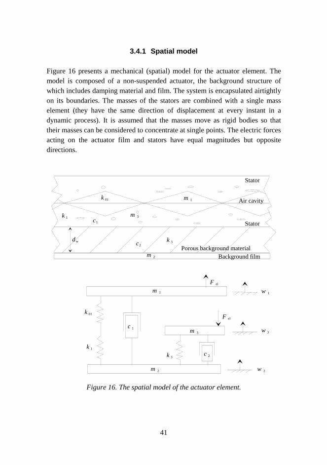
3.4.1 Spatial model

Figure 16 presents a mechanical (spatial) model for the actuator element. Themodel is composed of a non-suspended actuator, the background structure ofwhich includes damping material and film. The system is encapsulated airtightlyon its boundaries. The masses of the stators are combined with a single masselement (they have the same direction of displacement at every instant in adynamic process). It is assumed that the masses move as rigid bodies so thattheir masses can be considered to concentrate at single points. The electric forcesacting on the actuator film and stators have equal magnitudes but oppositedirections.

m 1

m 2 w 2

m 1

m 2

k 3

k 3

m 3 w 3

m 3

k 1

k 1

k 01

c 1

c 2

k 01

c2

c1

w 1

Background filmPorous background material

Stator

Stator

Air cavity

d w

F el

F el

Figure 16. The spatial model of the actuator element.

42

The quantities

m1, m2, m3 are the masses of the actuator film, the combined background filmand background material (including 1/3 part of the mass of theporous spring material) and the stator respectively,

k01, k1, k3 are the spring constants caused by initial tension of the actuatorfilm, the elasticity of the air (air cavity) and the dynamical stiffnessof the porous background material (k2 is the combined effect of k01

and k1),

c1 is the common damping coefficient (related to flow resistance) ofthe stator and background material,

c2 is the damping coefficient, and

dw the thickness of the porous background material.

Because air flows through the stator material, the air spring has no effect. Thestators and background film are supposed to be totally rigid. In reality, bothelements have some elasticity.

3.4.2 Modal model

The operation of the system is described as a set of vibration modes (naturalfrequencies with corresponding vibration mode shapes and modal dampingfactors). The solution describes the various ways in which the actuator elementis capable of vibrating naturally or without external forcing or stimulus. Mass(M) -, stiffness (K) -, damping (C) - and force matrices (F) for the systemillustrated in Figure 16 are the following (the damping coefficients c areassumed to be equal):

M K C F=�

�

��

�

�

��

=− −

− + −−

�

�

��

�

�

��

=−−

− −

�

�

��

�

�

��

= ⋅ −�

�

��

�

�

��

mm

m

k k kk k k k

k k

c cc c

c c c

1

2

3

2 2 1

2 2 3 3

3 3

0 00 00 0 0

00

2

11

0 F '

(21)

The characteristic values of the system, natural frequencies and characteristicvector matrices are calculated by solving the characteristic equation H(f) =

43

K – ω2(f)⋅M [34]. Table 2 includes the calculated values of natural frequenciesof various different modifications compared to the basic situation (case 0) andthe changes performed to the initial values (if no changes are made, the valuesare the same as in case 0). Because the system is non-suspended, the first modeis characterized by transfer and its natural frequency is in every case 0 Hz andthus not included in the table. The natural frequencies are very sensitive to theslightest changes in the parameters of the system which is very usual withmechanical constructions.

Table 2. Natural frequencies and modified mechanical parameters.

Case Naturalfrequencies

(Hz)

Depth(mm)

Masses(kg m-2)

Spring constants(kg m-2 s-2)⋅⋅⋅⋅106

f2 f3 dw m1 m2 m3 k01 k2 k3

0 302 914 50 0.042 1.01 3.96 3.3 1.3 3.01 47 947 - - 0.34 - - - 0.032 896 2110 - - 3,01 - - - 3003 237 716 100 - 2.01 - - 0.83 -4 35 729 100 - 0.68 - - 0.83 0.035 709 1785 100 - 6.01 - - 0.83 3006 210 608 150 - 3,01 - - 0.60 -7 30 616 150 - - - - 0.60 0.038 605 1663 150 - 9,01 - - 0.60 3009 394 1117 25 - 0.51 - - 1.9 -

10 61 1188 25 - 0,18 - - 1.9 0.0311 1070 2642 25 - 1,51 - - 1.9 30012 235 513 100 0.084 2.01 3.92 - 0.83 -13 238 1006 100 0.021 2.01 3.98 - 0.83 -14 237 716 100 - 2.005 - - 0.83 -15 237 715 100 - 2.02 - - 0.83 -16 274 716 100 - 2.01 1.98 - 0.83 -17 216 716 100 - 2.01 7.92 - 0.83 -18 141 3453 12.5 - 0,76 - 0.033 0.033 30019 141 412 25 - 0,51 - 0.033 0.033 -20 59 159 25 - 0,18 - 0.033 0.033 0,0321 141 2637 25 - 1,51 - 0.033 0.033 30022 366 484 25 - 0,51 - 0.33 0.31 -23 140 309 - - - - 0.033 0.033 -24 139 1785 100 - 6.01 - 0.033 0.032 300

44

The directions and amplitudes of the mass elements vary in different cases.Figure 17 illustrates the main modal forms of some cases. The basic case (firstmode, solid line), for example, illustrates the transfer of the structure. At thesecond mode (dotted line), all mass elements move to the same direction withdifferent relative amplitudes. At the third mode, the actuator film and statorsmove upwards and the background film downwards.

1 2 30.5

0

0.5

1

1.51.00000

0.23672

X M1< >

j

X M2< >

j

X M3< >

j

3.000001.00000 j

1 2 32

0

2

43.85754

1.00000

X M1< >

j

X M2< >

j

X M3< >

j

3.000001.00000 j

Figure 17. The main modal forms of the basic case and case 23, respectively.

3.4.3 Response model

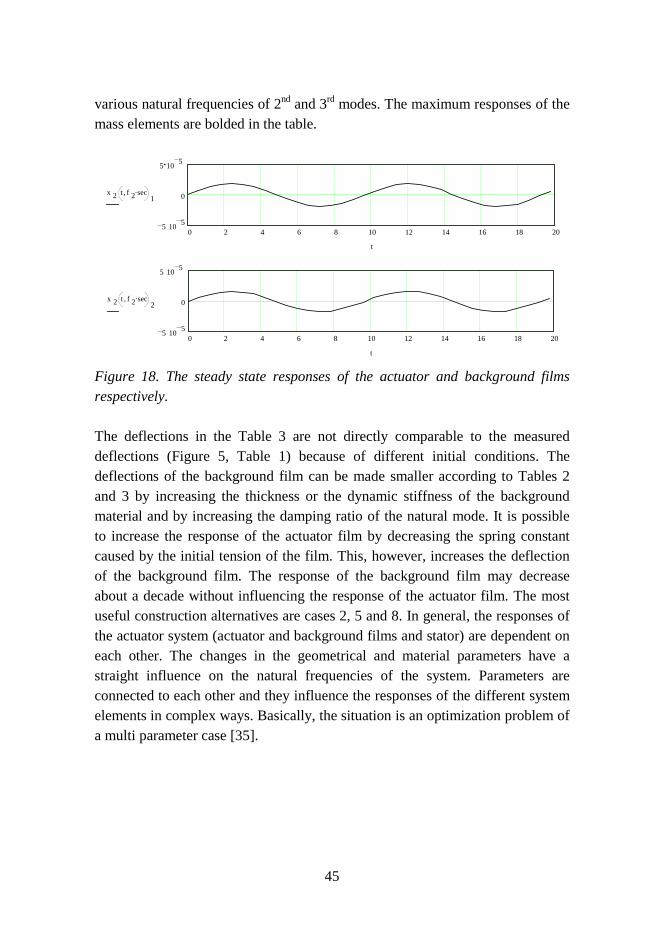
Figure 18 presents the steady state responses (2nd mode, 2nd natural frequency) ofthe actuator and background films in time domain (vibration of the masselements under condition of time harmonic excitation). Table 3 shows themaximum responses of the actuator and background films and the stator for

45

various natural frequencies of 2nd and 3rd modes. The maximum responses of themass elements are bolded in the table.

0 2 4 6 8 10 12 14 16 18 205 10 5

0

5 10 5

x 2 ,t .f 2 sec1

t

0 2 4 6 8 10 12 14 16 18 205 10 5

0

5 10 5

x 2 ,t .f 2 sec2

t

Figure 18. The steady state responses of the actuator and background filmsrespectively.

The deflections in the Table 3 are not directly comparable to the measureddeflections (Figure 5, Table 1) because of different initial conditions. Thedeflections of the background film can be made smaller according to Tables 2and 3 by increasing the thickness or the dynamic stiffness of the backgroundmaterial and by increasing the damping ratio of the natural mode. It is possibleto increase the response of the actuator film by decreasing the spring constantcaused by the initial tension of the film. This, however, increases the deflectionof the background film. The response of the background film may decreaseabout a decade without influencing the response of the actuator film. The mostuseful construction alternatives are cases 2, 5 and 8. In general, the responses ofthe actuator system (actuator and background films and stator) are dependent oneach other. The changes in the geometrical and material parameters have astraight influence on the natural frequencies of the system. Parameters areconnected to each other and they influence the responses of the different systemelements in complex ways. Basically, the situation is an optimization problem ofa multi parameter case [35].

46

Table 3. The maximum responses of the actuator elements.

2nd mode 3rd mode

2nd natural freq. 3rd natural freq. 2nd natural freq. 3rd natural freq.Actuator film

Basic case Background filmStator

1,9⋅10-5

1,7⋅⋅⋅⋅10-5

4,5⋅⋅⋅⋅10-6

3,8⋅10-8

3,4⋅10-8

9,0⋅10-9

1,0⋅10-5

4,7⋅10-7

1,1⋅10-8

3,7⋅⋅⋅⋅10-4

1,7⋅10-6

4,0⋅10-7

Actuator filmCase 1 Background film

Stator

2,5⋅10-6

2,5⋅10-6

2,5⋅⋅⋅⋅10-7

1,8⋅10-9

1,8⋅10-9

1,8⋅10-10

4,5⋅10-7

5,6⋅10-8

1,2⋅10-11

3,3⋅⋅⋅⋅10-4

4,1⋅⋅⋅⋅10-5

8,7⋅10-9


Stator

3,9⋅⋅⋅⋅10-4

1,7⋅⋅⋅⋅10-6

2,9⋅⋅⋅⋅10-6

1,4⋅10-6

5,8⋅10-9

1,0⋅10-8

3,6⋅10-9

1,7⋅10-8

1,3⋅10-8

1,2⋅10-7

5,4⋅10-7

4,1⋅10-7


Stator

1,1⋅10-5

9,4⋅⋅⋅⋅10-6

4,8⋅⋅⋅⋅10-6

1,5⋅10-8

1,3⋅10-8

7,0⋅10-9

1,4⋅10-5

3,2⋅10-7

1,3⋅10-8

3,5⋅⋅⋅⋅10-4

7,9⋅10-6

3,1⋅10-7


Stator

1,2⋅10-5

1,2⋅⋅⋅⋅10-6

2,1⋅⋅⋅⋅10-7

9,1⋅10-10

9,0⋅10-10

1,6⋅10-10

4,4⋅10-7

2,8⋅10-8

1,0⋅10-11

1,6⋅⋅⋅⋅10-5

1,0⋅10-6

3,7⋅10-10


Stator

3,5⋅⋅⋅⋅10-4

1,3⋅⋅⋅⋅10-6

1,7⋅⋅⋅⋅10-6

1,3⋅10-5

4,7⋅10-9

6,4⋅10-9

7,9⋅10-10

4,3⋅10-9

6,5⋅10-9

1,6⋅10-9

8,6⋅10-9

1,3⋅10-8


Stator

7,8⋅10-6

6,9⋅⋅⋅⋅10-6

5,3⋅⋅⋅⋅10-6

9,0⋅10-9

7,9⋅10-9

5,6⋅10-9

1,8⋅10-5

2,6⋅10-7

1,4⋅10-8

3,2⋅⋅⋅⋅10-4

4,9⋅10-6

2,6⋅10-7


Stator

7,5⋅10-7

7,5⋅10-7

2,0⋅⋅⋅⋅10-7

5,1⋅10-10

5,1⋅10-10

1,4⋅10-10

4,6⋅10-7

1,9⋅10-8

9,6⋅10-12

3,2⋅⋅⋅⋅10-4

1,3⋅⋅⋅⋅10-5

6,7⋅10-9


Stator

3,3⋅⋅⋅⋅10-4

1,0⋅⋅⋅⋅10-6

1,2⋅⋅⋅⋅10-6

1,5⋅10-6

4,5⋅10-9

5,6⋅10-9

2,5⋅10-10

1,7⋅10-9

3,8⋅10-9

1,6⋅10-8

1,1⋅10-7

2,4⋅10-7


Stator

2,6⋅⋅⋅⋅10-5

2,3⋅⋅⋅⋅10-5

3,2⋅⋅⋅⋅10-6

3,6⋅10-8

3,1⋅10-8

4,3⋅10-9

6,2⋅10-6

5,8⋅10-7

9,1⋅10-9

8,2⋅10-6

7,7⋅10-7

1,2⋅10-8


Stator

5,3⋅⋅⋅⋅10-6

5,4⋅⋅⋅⋅10-5

3,0⋅⋅⋅⋅10-7

1,2⋅10-9

1,2⋅10-9

6,0⋅10-11

4,8⋅10-7

1,2⋅10-7

1,6⋅10-11

5,0⋅10-5

1,2⋅10-7

1,6⋅10-9


Stator

1,7⋅⋅⋅⋅10-4

6,4⋅10-7

1,6⋅⋅⋅⋅10-6

8,8⋅10-7

3,3⋅10-9

8,1⋅10-9

3,2⋅10-9

1,6⋅10-8

6,2⋅10-9

1,7⋅10-7

8,9⋅⋅⋅⋅10-7

3,4⋅10-7


Stator

2,7⋅10-5

2,1⋅⋅⋅⋅10-5

1,1⋅⋅⋅⋅10-5

8,4⋅10-8

6,5⋅10-8

3,5⋅10-8

1,6⋅10-5

7,6⋅10-7

6,1⋅10-8

3,5⋅⋅⋅⋅10-4

1,8⋅10-5

1,4⋅10-6


Stator

4,8⋅10-6

4,5⋅⋅⋅⋅10-6

2,4⋅⋅⋅⋅10-6

1,6⋅10-8

1,5⋅10-8

7,6⋅10-9

5,3⋅10-5

5,6⋅10-7

1,1⋅10-8

3,9⋅⋅⋅⋅10-5

4,2⋅10-7

8,0⋅10-9


Stator

1,1⋅10-5

9,9⋅⋅⋅⋅10-6

5,1⋅⋅⋅⋅10-6

1,5⋅10-8

1,3⋅10-8

7,0⋅10-9

1,4⋅10-5

3,2⋅10-7

1,3⋅10-8

3,5⋅⋅⋅⋅10-4

7,9⋅10-6

3,1⋅10-7

to be continued

47

continuesActuator film

Case 15 Background filmStator

1,1⋅10-5

9,7⋅⋅⋅⋅10-6

5,1⋅⋅⋅⋅10-6

1,5⋅10-8

1,3⋅10-8

6,9⋅10-9

1,4⋅10-5

3,2⋅10-7

1,3⋅10-8

3,5⋅⋅⋅⋅10-4

7,9⋅10-6

3,1⋅10-7

Actuator filmCase 16 Background film Stator

1,0⋅10-5

8,6⋅10-6

8,9⋅⋅⋅⋅10-6

1,7⋅10-8

1,5⋅10-8

1,5⋅10-8

1,7⋅10-5

3,8⋅10-7

3,1⋅10-8

3,5⋅⋅⋅⋅10-4

7,9⋅⋅⋅⋅10-5

6,4⋅10-7


1,2⋅10-5

1,1⋅⋅⋅⋅10-5

2,7⋅⋅⋅⋅10-6

1,4⋅10-8

1,3⋅10-8

3,3⋅10-9

1,3⋅10-5

2,9⋅10-7

5,5⋅10-9

3,5⋅⋅⋅⋅10-4

7,9⋅10-6

1,5⋅10-7


7,8⋅⋅⋅⋅10-3

6,9⋅⋅⋅⋅10-5

7,0⋅⋅⋅⋅10-5

3,7⋅10-6

3,2⋅10-8

3,3⋅10-8

2,1⋅10-11

1,1⋅10-8

2,4⋅10-9

1,4⋅10-8

8,7⋅10-6

1,7⋅10-6


8,0⋅⋅⋅⋅10-3

6,1⋅⋅⋅⋅10-5

6,2⋅⋅⋅⋅10-5

7,5⋅10-7

6,0⋅10-9

5,8⋅10-9

2,7⋅10-11

9,3⋅10-9

3,6⋅10-9

2,1⋅10-9

7,5⋅10-7

2,9⋅10-7


6,5⋅10-6

5,4⋅10-6

3,5⋅10-7

7,0⋅10-6

5,7⋅10-6

3,3⋅10-7

2,9⋅10-5

6,8⋅10-6

6,2⋅10-8

7,3⋅⋅⋅⋅10-3

6,8⋅⋅⋅⋅10-6

1,6⋅⋅⋅⋅10-5


7,9⋅⋅⋅⋅10-3

2,4⋅10-6

8,5⋅⋅⋅⋅10-5

4,2⋅10-5

1,3⋅10-8

4,5⋅10-7

2,3⋅10-7

1,8⋅10-6

2,2⋅10-7

2,1⋅10-5

1,6⋅⋅⋅⋅10-4

2,0⋅10-5


9,3⋅⋅⋅⋅10-4

2,6⋅⋅⋅⋅10-4

4,3⋅⋅⋅⋅10-5

1,5⋅10-5

4,2⋅10-6

7,0⋅10-7

4,8⋅10-5

1,3⋅10-5

1,1⋅10-6

6,3⋅10-4

1,7⋅10-4

1,5⋅10-5


Stator

8,8⋅⋅⋅⋅10-3

1,8⋅10-6

8,5⋅⋅⋅⋅10-5

1,0⋅10-4

2,3⋅10-8

1,1⋅10-6

4,5⋅10-7

1,8⋅10-6

4,4⋅10-7

4,4⋅10-5

1,7⋅⋅⋅⋅10-4

4,2⋅10-5


Stator

8,1⋅⋅⋅⋅10-3

3,4⋅⋅⋅⋅10-5

3,4⋅⋅⋅⋅10-5

1,1⋅10-6

4,6⋅10-9

4,6⋅10-9

1,7⋅10-11

2,8⋅10-9

4,2⋅10-9

9,2⋅10-10

1,5⋅10-7

2,3⋅10-7

48

4. Sound productionThe sound field radiated by a vibrator embedded in a fluid can be calculated ifthe normal velocity of its external boundary is known. When the ambient fluid isgas, such as air, the source response can be, more or less, approximated by its invacuo one [36]. The loading can be described quite easily, however, by an addedmass or by radiation impedance. Thus, in the presence of fluid loading, theapplied force encounters the sum of the mechanical impedance of the source andthe radiation impedance.

A plane, the linear dimensions of which are very large compared to thewavelength and vibrating with the same amplitude and phase over its entiresurface, produces a plane wave propagating perpendicularly to its surface [37].The distribution of the acoustic field around a vibrating surface with boundeddimensions is more complicated. The radiation properties of this type of anacoustic source will depend on the shape and dimensions of the surface, thedistribution of the vibration velocity over its surface, and the interaction betweenthe two sides of the plane. If the dimensions of a sound source are much smallerthan the wavelength of the sound being radiated, then the details of the surfacemotion are not important, and it will radiate exactly the same sound as any othersimple source with the same source strength [38].

If the vibrating surface is a rigid body (at a given instant vibration, velocity isconstant over the entire surface), the source is called a piston-membrane.Usually, the mode of vibration is more complicated than that of a piston, and itdepends on the manner of fixing the membrane, its elastic properties and thefrequency of vibrations. If the membrane is located in a free acoustic space, thefields on both sides interfere with each other, producing a certain resultant field.If the membrane is located in free space, but the radiation of one of its sides isentirely attenuated by means of an insulating box, then only one side of themembrane radiates, but the radiation may propagate over the entire space.

In the present chapter, the above mentioned consideration is applied to theoperation of the EMFi-actuator. The examination of the sound emission isrestricted to the far field and the medium is supposed to be homogenous,isotropic and at rest. The medium is also assumed to be thermally non-conductive fluid and to obey the linear stress-strain laws (Hooke’s laws). The

49

acoustic pressure generated outside the source is assumed to be small enough sothat the first-order equations of sound are valid in the region outside the source[39]. A Sommerfield condition (or any equivalent condition) is assumed for thesound pressure field. This means that the boundary condition at infinity enablesno reflection so that only the outgoing waves exist.

4.1 Actuator in free acoustic field

The radiation resistances of the plane monopole and dipole sources at lowfrequencies, respectively, are [Appendixes D and E]

Ra

crm =πρ ω0

2 4

02 and R

acrd =

227

04 6

03

πρ ω(22)

whereρ0 is the density of the air,ω is the angular frequency, andc0 is the velocity of the sound.

The rectangular radiator element is accounted as a circular membrane of radiusa. The radius is approximated from the area of the element a = (DL/π)½ where Dand L are the dimensions of the rectangular membrane. Radiation resistances aredependent on the frequency of excitation, the properties of the actuator structureand the medium into which the sound is radiated. The sound power, radiated byan actuator panel vibrating with a spatial mean square value of velocity U0, is bythe definition related to the radiation resistance Rrad [40]. The radiated soundpowers of the monopole and dipole sources at low frequencies, respectively, are

Π m rmU R=12 0

2 Π d rdU R=12 0

2 (23)

The monopole source is assumed to be functioning as an encapsulated disk, andthe dipole source as a free vibrating disk. Sound pressure amplitudes at lowfrequencies and on axis one meter from the source are correspondingly

P c U kaaxm =14 0 0 0

2ρ P c U k aaxd =16 0 0 0

2 3ρ (24)

50

4.1.1 Constant velocity distribution

The velocity amplitude of vibration U0, normal to the radiator surface, is relatedto the deflection of the membrane, U0 = ωξ0e, where ξ0e is an average deflectionof the membrane. At 23 Volt signal voltage the average deflection is calculatedfrom the values in Table 1. The emitted sound power levels of monopole anddipole sources into the far field at low frequencies, when the velocitydistribution of the actuator film is assumed to be constant (piston source) [seeAppendix A], are presented in Figure 19.

0 100 200 300 400 500 600 700 800 900 10000

10

20

30

40

50

60

70

80

90

100

Frequency/Hz

Soun

d po

wer

leve

l/dB

100

0

L Wm f( )

L Wd f( )

1 103.50 f

Figure 19. Sound power levels of monopole and dipole sources at lowfrequencies.

The frequency when the sources radiate sound equally effectively is 680 Hz. Athigher frequencies the dipole source (dotted line) emits more sound power thanthe monopole source. In frequencies less than 300 Hz, the radiated sound powersof both sources diminish intensively. The decrement in the radiated power ismore significant for the dipole source. The sound pressure levels of monopoleand dipole sources at low frequencies at the distance of one meter from thesources on their axis are presented in Figure 20.

51

0 100 200 300 400 500 600 700 800 900 10000

20

40

60

80

100

Frequency/Hz

Soun

d pr

essu

re le

vel/d

B84.081

6.019

SPL m f( )

SPL d f( )

1 103.50 f

Figure 20. Sound pressure levels of monopole and dipole sources.

At high frequencies the dipole source produces more sound pressure into the farfield than the monopole source. This occurs when the frequency exceeds 800Hz. The frequency change is related to the area of the dipole actuator so thatwhen the area increases, the frequency decreases. This is natural because, in thecase of a dipole source, the effect of an acoustical short circuit also decreaseswhen the area increases. The large dipole actuators emit thus more sound power(and produce higher pressure levels) into the far field than the monopole sources.

4.1.2 Frequency dependent velocity distribution

In reality the vibration velocity of the actuator film is dependent on thefrequency according to Figure 5 and Table 1. By using this data and theassumptions made in chapter 4.1.1 concerning the spatial vibration distributionon the membrane, the sound power levels of monopole and dipole sources are aspresented in Figure 21. The solid lines in the figure present the curves of Figure19, respectively, for comparison reasons. It is evident, according to Figure 21,that the arithmetic average of the vibration deflection can replace the frequencydependent vibration of the actuator film satisfactorily in the frequency domainmost of the time when evaluating the radiated sound power of the monopole anddipole actuators.

52

0 100 200 300 400 500 600 700 800 900 10000

10

20

30

40

50

60

70

80

90

100

Frequency/Hz

Soun

d po

wer

leve

l/dB

100

0

L Wm f( )

L Wd f( )

L Wmmitb f( )

L Wdmitb f( )

1 103.50 f

Figure 21. Sound power levels of monopole and dipole sources.

4.1.3 Sinusoidal spatial velocity distribution

The axial sound pressure of actuator membrane at low frequencies at a distance rwith a spatial (sinusoidal) acceleration distribution is [41]

p rU LD e

r n mm n

n m jkr

( )( )

( )( ),=

−+ +

= =+ −2 10 0

3 12

12

ρπ

0,1,... (25)

where

U0 is the average vibration velocity amplitude,

L is the width of the actuator element,

D is the length of the actuator element, and

m, n are integers.

53

The sound pressure levels on the axis of the sound source at one meter from theradiating surface with sinusoidal acceleration distribution are illustrated inFigure 22. The first seven addended terms are taken into the calculation. Thevalues are compared to the sound pressure levels emitted by a constant velocityactuator and an actuator whose vibration velocity depends on the frequency.

0 100 200 300 400 500 600 700 800 900 100030

40

50

60

70

80

90

Frequency/Hz

Soun

d pr

essu

re le

vel/d

B

82.053

30.012

SPL m f( )

SPL mmitb f( )

SPL mJF f( )

1 103.50 f

Figure 22. Sound pressure levels of different actuator sources.

The solid line in the figure presents the curve of Figure 19, and the dotted linethat of Figure 21 for monopole sources, respectively, for comparison reasons.The arithmetic average of the vibration deflection is satisfactorily comparable tothe spatially dependent vibration of the actuator film in the frequency domainwhen evaluating the produced sound pressure levels. This is what it should bebecause when the dimensions of a sound source are much smaller than thewavelength of the sound being radiated, the details of the surface motion are notimportant anymore.

4.1.4 Effect of impedance loading

The vibration velocity of the actuator film is also influenced by its externalimpedance in reality, especially by the flow resistance of the stator materialaccording to equation (8) (see Figure 3). The effect of outward impedance on the

54

produced sound power of monopole source, compared to the situation whenthere is no resistive load caused by the flow resistance of the stator or theradiation resistance of the ambient fluid, is illustrated in Figure 23. Theinfluence of impedances is minor, and they affect mainly at higher frequencies.Similar results are pertinent also to dipole source and produced sound pressurelevels of both sources.

0 100 200 300 400 500 600 700 800 900 10000

10

20

30

40

50

60

70

80

90

100

Frequency/Hz

Soun

d po

wer

leve

l/dB

100

0

L Wm f( )

L Wmimp f( )

1 103.50 f

Figure 23. Sound power levels of monopole sources.

4.2 Dipole actuator near the boundary layer

The radiation of sound by a source can be strongly affected by the impedance ofthe surrounding space. This stands for the acoustic properties of the ambientmedium, the geometry of the space occupied by this medium, and the type ofboundary conditions that are imposed at the boundaries of the surroundingspace. When the dipole actuator is installed on or very close to a plane boundary,its acoustical properties change. If the dimensions of the boundary are far largerthan a wavelength of the radiated sound, then the boundary can be considered aplane of infinite extent [42]. If the boundary is perfectly rigid, the acousticwaves generated by the source will reflect from this plane so that

�u n⋅ =� 0where

�u is the particle velocity and �n is the normal to the plane. The pressure

55

of the reflected wave and that of the incident wave are in phase and identical atthe boundary. Sound power of a dipole source which is installed on an absorbentmaterial (which is sited on an acoustically rigid boundary layer) in the half-spaceoccupied by the source is [Appendixes F and G]

( ) ( )( ) ( )

( )

( )( ) ( )

( )( ) �

�

�

�ςΓ−��

�

�

��

�

��

�

�

��

�

−−ςΓ

+

�

�

��

�

�

��

�

��

�

�

��

�

−+ςΓ−Γ+Π⋅=Π

322

222

sin4cos211sin2sin2

sin211cos2cos2131

23

kbkb

kbkbkbkb

kbkbkbkb

kbdddhs

(26)

where

Γ is the reflection factor of the absorbent material,

ς is the phase between the incident and reflecting wave,

b/2 is the thickness of the absorbent layer,

k is the wave number, and

Πd is the sound power of the single dipole source in the free field.

It is assumed here that the radiator is acoustically transparent for the reflectingwaves from the plane surface. This assumption is justified at low frequencieswhere the wavelength is much longer than the dimensions of the actuator. Whenthe value of Γ is one and ς is zero (acoustically rigid boundary layer), theequation can be reduced to a case of two oppositely phased dipole sourcesseparated at a distance b from each other. The sound power levels of the dipolesource on the boundary layer in function of thickness of the absorbent layer andfrequency as a parameter are illustrated in Figure 24. The lossy material used inthe calculations is rock wool (60 kg/m3). When the thickness of the absorbentmaterial is under 5 cm, the radiated sound power decreases strongly. When theabsorbent layer is thicker than that, the power level increases slowly. Thedifference between the emitted sound power levels of 5 cm and 10 cm absorbentlayers at 250 Hz is 7 dB. The main reason for the decrement in the radiatedsound power when the thickness of the absorbent layer decreases is thedestructive interference of the oppositely phased incident and reflected waves.

56

0 0.05 0.1 0.15 0.2 0.25 0.30

10

20

30

40

50

60

70

80

The thickness of the absorbent/m

Soun

d po

wer

leve

l/dB

63.639

0

L Wdd 250b2

,

L Wdd 300b2

,

L Wdd 350b2

,

0.351.5 10 3. b2

Figure 24. Sound power level of the dipole source.

Figure 25 illustrates the radiated sound power levels of the dipole source whichis installed on a 10 cm thick rock wool layer and that of two oppositely phaseddipole sources (upper curve, Appendix E) the distance between which is 20 cm.The power loss caused by the absorbent material is 5 dB at 50 Hz. Thedifferences in the radiated power levels increase at higher frequencies. Thechange in the increased power loss is 0.3 dB in the frequency range of 50 - 250Hz.

40 60 80 100 120 140 160 180 200 220 240 2600

10

20

30

40

50

60

70

80

Frequency/Hz

Soun

d po

wer

leve

l/dB

69.94

7.097

L Wdd f 0.2 m.,( )

L Wdd1 f 0.2 m.,( )

25050 f

Figure 25. Sound power levels of the dipole sources.

57

The radiated sound power level of the dipole source at 100 Hz when the flowresistance of the lossy material increases (the thickness of the absorbent layer is10 cm) is illustrated in Figure 26. The flow resistances (10 - 200)⋅103 Ns/m2

correspond cotton or rock wool material the thickness of which varies in thedensity range of 20 - 100 kg/m3 and 100 - 200 kg/m3, respectively. The changein the radiated sound power level in the above mentioned flow resistance rangeis 3.5 dB.

0 5 .104 1 .105 1.5.105 2 .10523

24

25

26

27

28

Flow resistance/kgm-3^s^-1

Soun

d po

wer

leve

l/dB

27.576

23.975

L Wdd2 100 0.1 m., Ξ´,( )

2 105.1 103. Ξ´

Figure 26. The increment in the sound power level of a dipole source.

The radiated sound power of the dipole source increases because the waves onthe boundary are not totally in an opposite phase as a consequence of theincreased flow resistance, and thus the influence of the acoustic short circuit issmaller.

4.3 Radiation pattern of the actuator

The EMFi-actuator actually consists of several membrane strips (N sections)which are located next to each other on the same plane (see Figure 1). Theseparate strips operate, in principle, as single line sources combined of severalunit piston sources locating side by side (see Figures H1 and H2 in Appendix H).

58

The produced sound pressure of the actuator located in infinite baffle at a certainfar field point is (Appendix H)

p r t jP H H eax ej t kr( , , ) ( ) ( ) ( )Φ = −θ φ ω (27)

θ=νφφ

φ

νν=θ

πρ

=

sin where)sinsin()sinsin(

=)(

and sin)( ,4

)(

21

212

000

kLkdkd

H

Hr

dkLUcrP

m

mN

em

ax

where

Pax is the axial pressure amplitude,

U0 is the average vibration velocity amplitude,

L is the width of the actuator element,

dm is the width of the actuator cell,

r is the distance to the observation point, and

N is the number of film strips on the actuator element.

The directional properties of the EMFi-actuator at 100 Hz, 1000 Hz and 5000 Hzare presented qualitatively in Figures 27 - 29.

M

Figure 27. Radiation pattern of the actuator at 100 Hz.

59

M


M


The major lobe in the radiation pattern narrows when the frequency increases.The amplitudes of the other lobes are minor compared to the major one. Themajor lobe corresponds to that portion of the radiation pattern with which thesource elements are essentially in phase.

60

4.4 The effect of boundary condition on the soundradiation

The boundary conditions of a vibrating element influence its sound powerradiation. The EMFi film is glued to the stator element so that the actuatorelement is composed of several single sound radiation cells (see Figure 1). Theconnection type of those cell strips to the boundaries of the stator is not purelyrigidly neither simply supported. The consideration of the radiation properties ofnatural modes of simply and rigidly supported panels basically applies to platestructures. The vibration distributions of simply supported plate and membraneare, however, equal [34]. On the other hand, because the EMFi material is nottotally free of bending stiffness (it does not behave like ideal membrane), theradiation properties of rigidly supported plate are studied for reference purposes.The following assumptions are made in the consideration:

• the cell strip is supposed to vibrate time harmonically in one of its eigenmodes

• the cell strip is located in infinite baffle

• the load of ambient fluid is neglected

• the consideration is made in far field.

The radiated sound powers of simply and rigidly supported panels are,respectively (see Appendixes I and J)

φθθ⋅�π�

π

−πβ−

πα

βα

πρ=Π

��

�

�

��

�

�

��

�

��

��

�

�

��

�

��

��

�

�

��

�

��

�

�

��

�

� dd

nmmnkabuc m

ssp sin2

0

2

0 11

2sincos

2sincos

4

2

22

2

300(28)

61

φθθββ

β

ββ

β

β

αα

α

αα

αππ

απρ

ddbk

bk

b

bkk

bk

ak

ak

a

akk

ak

kuc

yn

yn

ynyn

ynxm

xm

xmxm

xm

mrsp

sin2

sin

1

12

sin

2cos

2tanh

12

sin

1

12

sin

2cos

2tanh

2

0

2

0

14

2

22

22

22

22

2

00

��

�

�

��

�

�

��

�

��

��

��

�

�

��

�

��

��

��

��

��

��

��

��

�

�

��

��

��

�

�

��

��

��

��

��

��

��

��

��

��

��

��

��

��

�

�

��

��

��

��

−

++

+

⋅

−

++

� � ⋅

+

=Π

(29)

where

Πssp, Πrsp are the radiated sound powers of simply and rigidly supported cellstrips,

um is the velocity amplitude of the vibrating cell strip,

kxm, kyn are the structural wavenumbers to the x-, y- co-ordinate directions,

a, b are the dimensions of the cell strip, and

m, n are integers.

In the case of simply supported cell strip (equation 28), the odd modes arerelated to the cosine terms, and the even modes, correspondingly, to the sinusterms. The radiated sound power levels of some odd modes (m,n) of simply(dotted lines) and rigidly (solid lines) supported cell strips are illustrated inFigure 30.

62

50 100 150 200 250 300 350 40040

20

0

20

40

Frequency/Hz

Soun

d po

wer

leve

l/dB

50

28.088

L W f 1, 1,( )

L Wyoo f 1, 1,( )

L W f 3, 3,( )

L Wyoo f 3, 3,( )

L W f 7, 7,( )

L Wyoo f 7, 7,( )

L W f 9, 9,( )

L Wyoo f 9, 9,( )

40050 f

Figure 30. The radiated sound power levels of odd modes (m,n).

Both supporting types of the cell strips enable almost equal sound powerradiation so that the vibration modes (1,1) are clearly the most efficient singleradiators. The reason for the similarity of the sound radiation of the separatemodes is the vibration velocity distributions of the cell strip of both boundarytypes. The velocity distributions of simply and rigidly supported cell strips arepresented in equations 30 and 31 and for some modes in Figures 31 - 34,respectively [38, 40].

u um x

an y

bmωπ π

= ��

��

��

��sin sin (30)

( )( )

( )( )

( )( )

( )( )u u

k x

k a

k x

k a

k y

k b

k y

k bm

xm

xm

xm

xm

yn

yn

yn

ynω = −

�

��

�

�� −�

�

��

�

�

��

cosh

cosh ½

cos

cos ½

cosh

cosh ½

cos

cos ½(31)

63

S

Figure 31. Vibration velocity distribution of a rigidly supported cell strip ofmode (1,1).

N

Figure 32. Vibration velocity distribution of a simply supported cell strip ofmode (1,1).

64

S


N


The vibration velocity distributions of simply and rigidly supported cell strips ofodd modes are practically equal, and thus also the radiated sound powers of thecell strips are equal. The radiated sound power levels of some even modes (m,n)of simply and rigidly supported cell strips are illustrated in Figures 35 and 36.

65

50 100 150 200 250 300 350 400100

80

60

40

20

0

20

Frequency/Hz

Soun

d po

wer

leve

l/dB

4.301

95.583

L Wyee f 2, 2,( )

L Wyee f 4, 4,( )

L Wyee f 6, 6,( )

L Wyee f 8, 8,( )

L Wyee f 10, 10,( )

40050 f

Figure 35. The radiated sound power levels of even modes (m,n). Simple support.

50 100 150 200 250 300 350 40040

20

0

20

40

Frequency/Hz

Soun

d po

wer

leve

l/dB

50

29.911

L W f 2, 2,( )

L W f 4, 4,( )

L W f 6, 6,( )

L W f 8, 8,( )

L W f 10, 10,( )

40050 f

Figure 36. The radiated sound power levels of even modes (m,n). Rigid support.

66

The rigidly supported boundaries of the cell strip enable it to radiate moreeffectively sound power with the separate even modes compared to the simplysupported boundary condition. The reason for this distinction is the vibrationvelocity distributions of the differently supported cell strips. The vibrationvelocity distributions of simply and rigidly supported cell strips of even modes(2,2) and (4,4) are presented in Figures 37 - 40.

S


N


67

S


N


68

The odd modes are more effective sound radiators compared to the even modes.Because the adjacent subsections of the cell strip are separated by much less thana wavelength in the surrounding air, the air displaced outward by one subsectionmoves to occupy the space left by the motion of the adjacent subsections,without being compressed, and very little sound power is radiated. For evenmodes the number of the vibrating subsections of the cell strip, which are in theopposite vibration phase, is equal, and thus the radiated net sound powerdecreases. On the contrary, for odd modes there always exist subsections whichare out of opposite vibration phases and thus also radiate sound power. Theradiation resistances and sound radiation of plates with different boundaryconditions are presented in the references [43, 44, 45, 46, 47, 48].

4.5 The measurement vs. modelling results

Acoustical testing for a plastic panel actuator, sized 320 mm ⋅ 420 mm (seeFigure 1), has been carried out in a semianechoic room by using a PC-installedMLSSA 10 measuring system [31]. The measurements cover both free and half-free acoustic fields. In half-free field measurements, the measured actuator wasplaced on the floor of the chamber so that either 20 mm mineral wool or onlyspacers were used between the floor and the panel under measurement. The sidesof the actuator panel were left open and no enclosures or baffles were used in themeasurements on the floor. In the free field measurements, the panel was hungfrom the ceiling and only anechoic part of the impulse response of the timesignal (direct sound) was used in the results. The distance between the actuatorand detector was 1 meter.

The constant average deflection of the film predicts quite satisfactorily the soundproduction properties of the actuator (see chapters 4.1.1 - 4.1.4). Thus frequencyor spatial dependence of the velocity distribution of the actuator film are nottaken into consideration when comparing the modelling and measurementresults. Also the external impedance loading of the actuator is ignored in theexamination.

69

4.5.1 The free acoustic field

Figure 41 presents the delivered sound pressure levels of the actuator element at1 meter from the vibrating plane in the free acoustic field. The solid line with therectangle symbols is based on the measurement results. The dashed (crosssymbols) and dotted (diamond symbols) lines are based on the modelling resultsof the monopole and dipole type of radiation, respectively. The analytical resultsare calculated according to equation (24).

0 100 200 300 400 500 600 700 8000

10

20

30

40

50

60

70

80

Frequency/Hz

Soun

d pr

essu

re le

vel/d

B

80

0

SPLi

SPL di

SPL mi

80080 fi

Figure 41. Sound pressure levels in a free acoustic field.

The calculated sound pressure level values of a monopole source are almostequal to the measured values up to 240 Hz. The shape of the sound pressurelevel curve of the dipole type actuator is similar compared to the measuredvalues up to 600 Hz so that a constant 8 dB amplitude difference exists. Themeasured sound pressure levels are, however, normalized in such a way that thetotal sound pressure level is 94 dB and the amplitude values are thus not directlycomparable. The monopole source type of modelling describes the deliveredsound pressure output of the EMFi-actuator at low frequencies. The dipole type

70

of modelling describes the sound pressure production properties of the actuatorin a larger frequency range when the amplitude difference, based on thenormalization of the measurement results, is taken into consideration.

4.5.2 The half-free acoustic field

Figure 42 presents the sound pressure level values in a half-free sound field,based on the actuator element measurements, and the respective analyticalresults. As earlier, the analytical values are specified for a monopole and dipoletype of radiation. The modelling results are calculated according to equation (24)by taking the results of Appendix G into consideration. The solid line with therectangle symbols is based on the measurement results. The dashed (crosssymbols) and dotted (diamond symbols) lines are based on the calculation resultsof monopole and dipole type of radiation, respectively.

0 80 160 240 320 400 480 560 640 720 8000

10

20

30

40

50

60

70

80

90

100

Frequency/Hz

Soun

d pr

essu

re le

vel/d

B

92.6

0

SPLi

SPL di

SPL mi

80080 fi

Figure 42. Sound pressure level in a half-free acoustic field.

71

The monopole source type of modelling predicts the delivered sound pressurelevels of the measured actuator very accurately up to 600 Hz. The shape of thesound pressure level curve of the dipole type actuator is similar compared to themeasured values up to 240 Hz. The amplitude difference between the values ofthe measured and dipole type modelled curves is 12 dB. The monopole type ofsource modelling is more realistic in half-free acoustic fields because basicallyin dipole type of radiation, the destructive interference of the oppositely phasedincident and reflected waves do not decrease very effectively the radiated soundat low frequencies because of the absorption material under the actuator. At highfrequencies, the discrepancies between the modelling and measurement resultsin free and half-free acoustic fields arise from the fact that the externalimpedance loading of the actuator has been ignored in the examination.

4.5.3 The directivity of the actuator

The directivity of the actuator element has been measured at 15 degree intervalsin a half-free acoustic field. In measurements, a mineral wool the thickness ofwhich is 20 mm has been inserted between the EMFi panel and the floor. Thecalculated (see Appendix H) and measured sound pressure levels of the EMFi-actuator at angles of 0°, 30°, 60° and 90° degrees at low frequencies arepresented in Figures 43 and 44. The calculated results are based on equation (27).

0 100 200 300 400 500 600 70030

40

50

60

70

80

90

Frequency/Hz

Soun

d pr

essu

re le

vel

90

30

LP f 1, π, π,( )

LP f 1, π,π6

,

LP f 1, π,π3

,

LP f 1, π,π2

,

70080 f

Figure 43. Calculated sound pressure levels at different angles in a half-freeacoustic field.

72

0 80 160 240 320 400 480 560 640 720 80030

40

50

60

70

80

90

Frequency/Hz

Soun

d pr

essu

re le

vel/d

B90

30

SPL0i

SPL30i

SPL60i

SPL90i

80080 fi

Figure 44. Measured sound pressure levels at different angles in a half-freeacoustic field.

When the actuator panel is located near the boundary surface, radiation up to400 Hz is very uniform in all directions. The sound pressure level curves of themeasured and predicted values are very similar in every angle. The calculatedand measured polarn patterns of the EMFi-actuator panel at 120 Hz, 240 Hz and500 Hz at different angles are presented in Figures 45 and 46.

73

0

15

30

45

60

7590

105

120

135

150

165

180

195

210

225

240

255270

285

300

315

330

345

706050403020100

70

41.901

b 1 120 Hz. π, Φ,( )

b 1 240 Hz. π, Φ,( )

b 1 500 Hz. π, Φ,( )

Φ

Figure 45. Calculated polarn patterns in acoustic half-free field conditions.

0

15

30

45

60

7590

105

120

135

150

165

180

195

210

225

240

255270

285

300

315

330

345

706050403020100

70

38

SPL120

SPL240

SPL500

f

Figure 46. Measured polarn patterns in acoustic half-free field conditions.

74

The radiation patterns of the actuator element are relatively round and resemblethe radiation patterns of the monopole source. The measured and predictedvalues are very similar in every angle. The radiation patterns produced by apiston-type actuator differ from the idealized patterns to some extent. Onereason for this discrepancy is that the area of the baffle in which the actuator ismounted is necessarily finite. At high frequencies, even a baffle of small lineardimensions corresponds quite closely to an ideal infinite baffle, but at lowfrequencies each element of the piston will not radiate with hemisphericaldivergence. In addition, radiation from the back of the actuator may propagateinto the region in front of the actuator so that the resulting radiation patternapproximates that of a dipole source rather than that of a piston in an infinitebaffle. Another reason for discrepancy is that the material of an EMFi-actuatormembrane is not perfectly rigid. Driving the actuator at its centre establishes ahigher velocity amplitude in the inner parts of the film than near its rim, and athigh frequencies, the film may even vibrate in normal modes. Under thesecircumstances, U0 in equation (H3) may become a complex function of the radialdistance and angle, and hence, must be considered a variable in the integration.

4.6 Methods to influence the sound production of theactuator

4.6.1 Change in the deflection of the film

The emitted sound power to the far field depends on the velocity (or thedeflection) amplitude of the film according to the equations (23 and 26). Thechange in the deflection of the membrane depends on the membrane tension andthe applied signal voltage. The sound power levels of monopole and dipolesources, related to normalized deflection and at parameter frequencies 50 Hz(solid line), 100 Hz (dotted line) and 150 Hz (dot-dashed), are illustrated inFigures 47 and 48.

75

0 1 2 3 4 5 6 7 8 9 1030

40

50

60

70

80

Normalized deflection

Soun

d po

wer

leve

l/dB

76.867

37.782

L Wmζ ζ1 50,( )

L Wmζ ζ1 100,( )

L Wmζ ζ1 150,( )

9.8990.99 ζ1ζ 0e

Figure 47. Sound power levels of a monopole source as a function of filmdeflection.

0 1 2 3 4 5 6 7 8 9 100

10

20

30

40

50

60

70

80

Normalized deflection

Soun

d po

wer

leve

l/dB

63.666

15.039

L Wdζ ζ1 50,( )

L Wdζ ζ1 100,( )

L Wdζ ζ1 150,( )

9.8990.99 ζ1ζ 0e

Figure 48. Sound power levels of a dipole source as a function of film deflection.

The radiated sound power levels of the monopole and dipole type actuatorsincrease 6 dB when the magnitude of the deflection is doubled, and 20 dB whenthe magnitude of the deflection is ten times the original one. The increment doesnot depend on the frequency, and it is equal for both source types.

76

4.6.2 The change in the area of the radiator element

The delivered sound pressure levels of monopole and dipole type actuatorsrelated to the normalized area at frequencies 50 Hz (solid line), 100 Hz (dottedline) and 150 Hz (dot-dashed) are illustrated in Figures 49 and 50. Soundpressure levels of a monopole source increase 6 dB when the area of the actuatorelement is doubled. For the dipole source, the increment in the sound pressurelevels is 9 dB, correspondingly. The increment does not depend on the frequencyand it is not equal for the source types. When the increment of the actuator areais tenfold compared to the original area, the sound pressure levels of a monopoletype source increase 20 dB and a dipole type source 30 dB, correspondingly.

It is possible to increase the delivered sound pressure of the actuator element tothe acoustic far field and to lower the frequency where the source types are equalradiators by increasing the area of the actuator. Figure 51 presents the deliveredsound pressure levels of monopole and dipole sources when the areas of theactuator panels are 4 m2. In this case, the dipole type actuator is a more effectiveradiator almost in the entire examined frequency range.

1 2 3 4 5 6 7 8 9 1020

30

40

50

60

70

80

Normalized area

Soun

d pr

essu

re le

vel/d

B

80

20

SPL m1 A1 50,( )

SPL m1 A1 100,( )

SPL m1 A1 150,( )

101 A1A

Figure 49. Sound pressure levels of a monopole source as a function of actuatorarea.

77

1 2 3 4 5 6 7 8 9 100

10

20

30

40

50

60

70

80

Normalized area

Soun

d pr

essu

re le

vel/d

B80

0

SPL d1 A1 50,( )

SPL d1 A1 100,( )

SPL d1 A1 150,( )

101 A1A

Figure 50. Sound pressure levels of a dipole source as a function of actuatorarea.

0 100 200 300 400 500 600 700 800 900 100050

60

70

80

90

100

110

120

130

Frequency/Hz

Soun

d pr

essu

re le

vel/d

B

130

50.229

SPL d f( )

SPL m f( )

1 103.50 f

Figure 51. Sound pressure levels of large dipole and monopole actuators.

78

Increment in the emitted sound power/pressure, based on the larger actuatorarea, is related to the change in the radiation resistance value of the actuatorelement. The radiated acoustic energy is counted as losses for the vibratingelement itself. Those losses increase when the larger actuator area adds to itsradiation resistance. At low frequencies, the acoustic short circuit decreases theradiation efficiency of the dipole type actuator. When the area of the dipolesource enlarges, the effect of the acoustic short circuit diminishes, and theactuator radiates sound more effectively.

4.6.3 The interaction of the sources

The sound field radiated by an actuator is often affected by neighbouringsurfaces or sound sources considerably. Two sound sources interact with eachother when they are close or when low frequencies are considered [38]. For asource with a characteristic dimension a, vibrating at an angular frequency ω =ck and located at a nominal distance b from another source, the far field pressureand the net acoustic power output depend on kb and a/b. The state of vibration ofthe vibrator element is assumed to be independent of b, and the single monopoleor dipole type actuators to function like the ones discussed before. The radiatedsound powers of two interacting monopole and dipole sources are, respectively([39], Appendix F)

( )Π Πmm m

kbkb

= ⋅ ⋅ +�

��

�

��2 1

sin(32)

( ) ( )Π Πdd d kb k bkb

k bkb= ⋅ ⋅ + −�

��

�� +

�

�

��6

13

11

2 22 2 2 2sin cos (33)

In the limit a/b<<1, that is, when the distance between the sources is largecompared to the dimensions of a single vibrator, the total acoustic field is wellapproximated by the superposition of those fields resulting from separateconsideration of the two sources. The sound power levels of interactingmonopole and dipole sources are illustrated in Figures 52 and 53. Theparameters of the curves are the distance 0.1 m (thin solid line), 0.5 m (dottedline) and 1 m (dot-dashed line). The thick dashed lines present the radiatedsound power levels of single monopole or dipole sources, respectively.

79

40 60 80 100 120 140 160 180 200 220 240 26030

40

50

60

70

80

Frequency/Hz

Soun

d po

wer

leve

l/dB

71.773

37.87

L Wmm f 0.1,( )

L Wmm f 0.5,( )

L Wmm f 1,( )

L Wm f( )

25050 f

Figure 52. Sound power levels of two interacting monopole sources at lowfrequencies.

40 60 80 100 120 140 160 180 200 220 240 26010

20

30

40

50

60

70

Frequency/Hz

Soun

d po

wer

leve

l/dB

62.948

15.126

L Wdd f 0.1,( )

L Wdd f 0.5,( )

L Wdd f 1,( )

L Wd f( )

25050 f

Figure 53. Sound power levels of two interacting dipole sources at lowfrequencies.

At low frequencies, or when the two actuators are located close to each other,the sound power level increases 6 dB compared to that of a single source. Athigh frequencies, the increment is, correspondingly, 3 dB. In the latter case, the

80

increment in the total sound power level equals that of two single sourceswithout any interaction. The interaction effect of the dipole sources disappears atlower frequencies than that of the monopole sources. At low frequencies, theincrement of the sound power levels of two interacting sources equals inmagnitude the situation when the deflection increment of the single actuatormembrane is doubled. Figure 54 illustrates the normalized sound powers ofinteracting monopole (solid line) and dipole (dotted line) sources. The soundpower of the two interacting sources is four times as large as that of the singlesource at low frequencies or when the sources are located close to each other.

0 1 2 3 4 5 6 7 8 9 100

1

2

3

4

k(f)*b

Nor

mal

ized

soun

d po

wer

3.99667

0.508303

Π nmm( )s

Π ndd( )s

100.1 s

Figure 54. The normalized sound powers of interacting monopole and dipoleactuators.

4.6.4 The change in the dimensions of the cell strip

The dimensions of the actuator cell affect the power the single vibration moderadiates to the acoustic far field. The radiated sound power levels of the modes(1,1) and (2,2) of the rigidly supported cell strips are illustrated in Figures 55 -58. The actuator cell width and length are the parameters of the curves. Thelengths or widths of the actuator cell are changed from 1/4 part to a fourfold ofthe original dimensions. The present actuator dimensions (thick dashed lines inthe figures stand for the reference dimensions presented in Appendix A) seem tobe acceptable. When the dimensions of the actuator cell are smaller than in thereference case, the emitted sound power decreases. When the dimensions of the

81

actuator cell are, correspondingly, larger, the radiated sound power does notsignifically increase. The sound power level values, concerning the smallelement lengths in Figure 56, are not pertinent at high frequencies. The samestatement concerns also the radiated sound power levels of the mode (2,2) of arigidly supported cell strip presented in Figure 58.

50 100 150 200 250 3000

10

20

30

40

50

Frequency/Hz

Soun

d po

wer

leve

l/dB

49.497

4.766

L W f 1, 1, a,b4

,

L W f 1, 1, a,b2

,

L W f 1, 1, a, b,( )

L W f 1, 1, a, 2 b.,( )

L W f 1, 1, a, 4 b.,( )

30050 f

Figure 55. The radiated sound power of mode (1,1) of a rigidly supportedactuator cell having the cell width as a parameter.

82

50 100 150 200 250 3000

10

20

30

40

50

60

70

Frequency/Hz

Soun

d po

wer

leve

l/dB

62.122

5.955

L W f 1, 1,a4

, b,

L W f 1, 1,a2

, b,

L W f 1, 1, a, b,( )

L W f 1, 1, 2 a., b,( )

L W f 1, 1, 4 a., b,( )

30050 f

Figure 56. The radiated sound power of mode (1,1) of a rigidly supportedactuator cell having the cell length as a parameter.

50 100 150 200 250 3005

0

5

10

15

20

25

30

35

Frequency/Hz

Soun

d po

wer

leve

l/dB

33.22

1.742

L W f 2, 2, a,b4

,

L W f 2, 2, a,b2

,

L W f 2, 2, a, b,( )

L W f 2, 2, a, 2 b.,( )

L W f 2, 2, a, 4 b.,( )

30050 f

Figure 57. The radiated sound power of mode (2,2) of a rigidly supportedactuator cell having the cell width as a parameter.

83

50 100 150 200 250 30010

0

10

20

30

40

50

60

Frequency/Hz

Soun

d po

wer

leve

l/dB

59.859

1.468

L W f 2, 2,a4

, b,

L W f 2, 2,a2

, b,

L W f 2, 2, a, b,( )

L W f 2, 2, 2 a., b,( )

L W f 2, 2, 4 a., b,( )

30050 f

Figure 58. The radiated sound power of mode (2,2) of a rigidly supportedactuator cell having the cell length as a parameter.

The simply supported actuator cells enable more effective sound power radiationat odd and even modes when the dimensions are larger than the originaldimensions of the actuator cell (see Appendix A). The radiated sound powerlevels of the modes (1,1) and (2,2) of simply supported actuator cells areillustrated in Figures 59 - 62. The actuator cell width and length are the curveparameters. The even modes are very poor sound radiators. In that case, changesin the dimensions of the actuator cell have minor influence on the emitted totalsound power. Doubling the element width or length increases, however, theemitted sound power of odd modes by 6 dB. Correspondingly, the fourfoldincrement of the width or length of the actuator cell increases the radiated soundpower of odd modes by 12 dB.

84

50 100 150 200 250 3000

10

20

30

40

50

60

Frequency/Hz

Soun

d po

wer

leve

l/dB

56.654

1.934

L Wyoo f 1, 1, a,b4

,

L Wyoo f 1, 1, a,b2

,

L Wyoo f 1, 1, a, b,( )

L Wyoo f 1, 1, a, 2 b.,( )

L Wyoo f 1, 1, a, 4 b.,( )

30050 f

Figure 59. The radiated sound power of mode (1,1) of a simply supportedactuator cell having the cell width as a parameter.

50 100 150 200 250 3000

10

20

30

40

50

60

Frequency/Hz

Soun

d po

wer

leve

l/dB

56.654

1.934

L Wyoo f 1, 1,a4

, b,

L Wyoo f 1, 1,a2

, b,

L Wyoo f 1, 1, a, b,( )

L Wyoo f 1, 1, 2 a., b,( )

L Wyoo f 1, 1, 4 a., b,( )

30050 f

Figure 60. The radiated sound power of mode (1,1) of a simply supportedactuator cell having the cell length as a parameter.

85

50 100 150 200 250 30080

60

40

20

0

20

Frequency/Hz

Soun

d po

wer

leve

l/dB

13.979

71.912

L Wyee f 2, 2, a,b4

,

L Wyee f 2, 2, a,b2

,

L Wyee f 2, 2, a, b,( )

L Wyee f 2, 2, a, 2 b.,( )

L Wyee f 2, 2, a, 4 b.,( )

30050 f

Figure 61. The radiated sound power of mode (2,2) of a simply supportedactuator cell having the cell width as a parameter.

50 100 150 200 250 30080

60

40

20

0

20

Frequency/Hz

Soun

d po

wer

leve

l/dB

13.979

71.912

L Wyee f 2, 2,a4

, b,

L Wyee f 2, 2,a2

, b,

L Wyee f 2, 2, a, b,( )

L Wyee f 2, 2, 2 a., b,( )

L Wyee f 2, 2, 4 a., b,( )

30050 f

Figure 62. The radiated sound power of mode (2,2) of a simply supportedactuator cell having the cell length as a parameter.

86

5. Sound power measurement of theactuator element

The measurement standard is applied to describe the installation, operation andenvironmental conditions under which the measured object must operate duringthe measurements. The measured value may be the average of measurements ofseveral equipment, or a calculated value of measurements under severaloperating conditions of equipment, or both. The essential feature is that themeasured value is the most probable sound emission value obtained whenapplying the given measurement standard [49]. If the manufacturer wishes thegiven sound emission value to have some predescribed certainty of acceptance inthe possible verification, he must regard the measurements and measured valuesstatistically. It is possible to calculate the confidence interval of the mean, usingany desired probability, from the mean of the measured values and from thestandard deviation of the reproducibility of the measurement method. The basicsound emission quantity used is the A-weighted sound power level.

One problem in using the basic sound power measurement standards (ISO 3740series) for comparison and evaluation purposes of sound power production ofequipment is the condition for the employment of the A-weighted standarddeviation. This problem concerns also the evaluation of the declaration values ofthe machinery and equipment [50]. For example ISO 3743-2 states in chapter1.3, Measurement uncertainty: “For a source which emits noise with a relatively‘flat’ spectrum in the 100 to 10 000 Hz frequency range, the A-weighted soundpower level is determined with a standard deviation of a mean value ofapproximately 2 dB” [51]. In present sound power measurement standards thereis, however, no definition for the “relatively flat spectrum”. Thus it is impossibleto know exactly in which situations one can consider equipment to emit sound“with a relatively flat spectrum” and in which situations the spectrum of theemitted sound has properties that cannot be considered to be in compliance withthe standard. There are at least three reasons to avoid the use of such a conceptas a “flat” spectrum:

• The uncertainties of the measurement standards in each one-third octave oroctave bands in engineering methods prohibit the estimation of “flatness” ofthe sound spectrum of equipment because of the quite large standard

87

deviations. In practice, the manufacturer should use the ISO precisionmethods to evaluate the flatness of the spectrum before carrying out anyuncertainty measurements.

• International standards already specify the character of sound allowable forthe method (steady, broad band, narrow band, etc.) [52]. There should be noother determinations for the character of sound.

• The character of the sound spectrum of the equipment should not influencethe manner of proceeding in general.

The A-weighted standard deviation of reproducibility for sound powermeasurements is currently given in standards ISO 3741 (0.5 dB), ISO 3743-1(1.5 dB), ISO 3743-2 (2 dB), ISO 3744 (1.5 dB), ISO 3746 (3-5 dB) ), ISO 3747(1.5 dB), ISO 9614-1 (4 dB) and ISO 9614-2 (1.5 or 4 dB) [52]. A method fordetermination of the A-weighted standard deviation of reproducibility for soundpower measurements of equipment in a more unambiguous manner is presentedin the following text.

5.1 Confidence interval

The confidence interval value K is chosen to account for the randommeasurement errors occurring under reproducibility conditions. For theprobability of acceptance of at least 95% in a possible subsequent verificationanother measurer, K is equal to [53]

K R= ⋅1645. σ (34)

where σR is the standard deviation of the reproducibility of the measurementmethod. The factor K is also the confidence interval of a normal distributionhaving the probability of 95% in a one-sided test for checking the upper limit.When considering a batch of equipment, the differences in sound emissionproperties of different equipment have to be taken into account. In this case,instead of using the standard deviation of the reproducibility of the measurementmethod, the total standard deviation is used, which is the combination of thestandard deviation of the reproducibility of the measurement method and the

88

standard deviation of production. The latter indicates the distribution of soundemission values of different equipment in a batch. The total standard deviation is

PRT22 σ+σ=σ (35)

where σR is the standard deviation of reproducibility and σP is the standarddeviation of production. K is now equal to

)(564.0514.1 TMTK σ−σ⋅+σ⋅= (36)

where σM is the reference standard deviation and K is the confidence interval ofa normal distribution with a probability of 93.5% in a one-sided case [53].

5.2 Determination of the combined standard deviation

The A-weighted standard deviation values given in the measurement standardsare based on the “flatness” of the spectrum emitted by the equipment. Because itis inconvenient to estimate whether or not the emitted sound is “flat”, it is betterto evaluate the A-weighted standard deviation of the reproducibility value fromthe single frequency band standard deviations given in the measurementstandards and from the measured sound emission values.

The following examination is based on the assumption that the results ofrepeated measurements with the same equipment are normally distributed. Foran arbitrary function Y = f(X1,X2,...,XN), the combined standard uncertainty of theestimate y (where y is the estimate of the measurand Y and thus the result of themeasurement) may be found from the accumulation law of probabilities.Because it is not possible to know exactly how the sound emission values ofdifferent frequency bands depend on each other, one must examine extremecases in which all frequency band values are independent or totally dependent,and thus determine the upper limit for the confidence interval value K.

89

5.2.1 Uncorrelated vs. totally correlated data in frequency bands

The combined standard uncertainty uc(y), when all input quantities areindependent of each other, is the positive square root of the combined varianceuc

2(y) which is given by [54]

�=

⋅��

��

�

∂∂=

N

ii

ic xu

xfyu

1

22

21 )()( (37)

( ) ( )u xN

x xi ii

N

=−

⋅ −=�

11

2

1(38)

where

f is the given function,

u(xi) is a standard uncertainty determined in equation (38),

xi is the measured value, and

x is the arithmetic mean value of N observations.

For a sum of A-weighted noise emission levels

��

�

�

��

�

�⋅=

+

=�

10

110lg10

ii axN

if (39)

where

ai is the A-weighting factor, and

xi is the sound emission value of the single frequency band.

The partial derivative of f with respect to x1 is

�=

+

+

=∂∂

N

i

ax

ax

iiix

f

1

10

10

10

1011

(40)

90

Corresponding expressions can be found for the partial derivative of f withrespect to x2, etc. When these partial derivatives of function f are inserted intoequation (37) the combined standard deviation is

( ) ( )( )

�

�

=

+

=

+⋅= N

i

ax

N

i

axi

cii

iixuyu

1

10/)(

1

210/

110

10)(

(41)

For the special case in which all the input estimates are completely correlated,the combined standard uncertainty uc(y) is the positive square root of thecombined variance uc

2(y) which is given by [54]

2

1

22 )()( �

�

��

�⋅��

�

�

�

∂∂= �

=

N

ii

ic xu

xfyu (42)

Proceeding as before, the combined standard deviation based on the sum of theA-weighted sound emission levels is

( )( )u y

u xc

x ai

i

N

x a

i

N

i i

i i

2

1 0

1

1 0

1

1 0

1 0( )

( ) /

( ) /=

⋅+

=

+

=

�

�

(43)

It is now possible to consider the characteristics of equations (41) and (43) in thefollowing different situations:

1) The single standard deviations of reproducibility are u(xi) = 0. The combinedstandard deviations are

0)()( 21 == yuyu cc (44)

as they should be.

91

2) The single standard deviations of reproducibility are similar while the soundemission levels for one-third octave or octave bands are not equal. Thecombined standard deviations are

( )u y uc

x a

i

N

x a

i

N

i i

i i

1

10 2

1

10

1

10

10( )

( ) /

( ) /= ⋅

+

=

+

=

�

�(45)

u y uc2 ( ) = (46)

where u = u(xi) is constant (≠ 0).

3) The single standard deviations of reproducibility are similar, as well as thesound emission levels for one-third octave or octave bands. The combinedstandard deviations are

( )u y uc

a

i

N

a

i

N

i

i

1

10 2

1

10

1

10

10( )

/

/= ⋅ =

=

�

�(47)

u y uc2 ( ) = (48)

where u = u(xi) is constant (≠ 0).

4) Sound emission levels for one-third octave or octave bands are similar, andthe single standard deviations of the reproducibility are not equal. Thecombined standard deviations are

( )u y c b u xc i ii

N

12

1( ) = ⋅ ⋅

=� (49)

( ) ( )( )u y c b u xc i ii

N

21

= ⋅ ⋅=� (50)

where ( )c a

i

Ni=

−

=� 10 10 1

1

/ and biai= 10 10/ are constants.

92

Considering the different ISO standards for standard deviations ofreproducibility of one-third octave bands, and supposing that the spectrum isflat, the combined standard deviations calculated from equations (49) and (50)are listed in Table 4. Also interlaboratory measurement results for a sourcewhich emits sound with a relatively “flat” spectrum in the 100 to 10 000 Hzfrequency range are listed in the same table [52].

Table 4. Standard deviations of reproducibility for a “flat” spectrum.

ISOStandard

Combined standarddeviation

A-weightedstandarddeviation

Classification of method

uc1 uc2

3741 0.46 1.76 ≤ 0.5 Precision3742 0.46 1.76 ≤ 0.5 Precision

3743-1 0.75 1.68 ≤ 1.5 Engineering3743-2 0.98 2.20 ≤ 2.0 Engineering3744 0.44 1.73 ≤ 1.5 Engineering3745 0.29 1.14 ≤ 1.0 Precision/Semi-anechoic3745 0.16 0.64 - Precision/Anechoic3746 - - ≤ 3 or ≤ 4 Survey3747 0.80 1.78 1.5 Engineering

9614-1 0.320.44

-

1.231.73

-

--4

PrecisionEngineering

Survey9614-2 0.44

-1.68

-1.54

EngineeringSurvey

In all cases uc1(y) ≤ uc2(y) (see Appendix K). The case where the input estimatesare completely correlated seems to give an upper limit for the combined standarddeviation. The calculated combined standard deviation values for the flatspectrum (50) are also quite congruent with the interlaboratory measurementresults (A-weighted standard deviation) when the single deviation values are

93

large. When the single deviation values are small, the combined standarddeviation value based on completely correlated input estimates seems to be morecongruent with the interlaboratory measurement result. In reality, the soundemission levels of different frequency bands are not totally correlated oruncorrelated. The “true” dependence is evidently between the two.

5.2.2 Confidence interval values based on the combined standarddeviation

The confidence interval value K for single equipment based on uncorrelated orcompletely correlated input estimates is now equal to

( )K u yc= ⋅1645 1. or ( )K u yc= ⋅1645 2. (51)

The confidence interval values for a batch of equipment can be calculated fromequations (36) where

( )σ σT c Pu y= +12 2 or ( )σ σT c Pu y= +2

2 2 (52)

5.3 Calculation examples

In order to compare the values estimated from the different combined standarddeviations stated above, some calculation examples are studied. The examplesare based on the spectrum of real measurements carried out according to the ISOstandards.

The one-third octave band sound power levels Lw of a fan (powered roofventilator) are shown in Figure 63. Laboratory measurements were performed incompliance with ISO 3741. The sound power levels are based on measurementsat 1466, 1454 and 1451 rpm speed of rotation.

94

102 103 1042 3 4 5 6 7 8 2 3 4 5 6 7 8 2

Frequency (Hz)

30

40

50

60

70

80

Soun

d po

wer

leve

l (dB

)

1465.8 1/min1454.3 1/min1451.4 1/min

Figure 63. One-third octave band sound power levels of a fan.

The confidence interval values of a normal distribution K are given in Table 5.The confidence intervals were calculated from equations (51), (41) and (43), andfrom a given A-weighted standard deviation value of reproducibility (ISO 3741)and equation (34).

Table 5. Confidence interval values of the normal distribution.

UncorrelatedEquation (41)

uc1/dB

CorrelatedEquation (43)

uc2/dB

Based on “flat”spectrum

ISO 3741/dB

K (1466 rpm) 0.80 2.92 0.82

K (1454 rpm) 0.79 2.74 0.82

K (1451 rpm) 0.77 2.62 0.82

95

The confidence interval values of a normal distribution K obtained from thecombined standard deviations uc1 (column 2 of Table 5) are quite near themeasured “flat” spectrum values (column 4) obtained from the measurementstandard, even when the examined spectra are not “flat” (see Figure 63).

The one-third octave band sound power levels of ventilation terminal equipmentare shown in Figure 64. Laboratory measurements were performed incompliance with ISO 3741. The sound power levels are based on measurementsat 1.7, 2.4 and 3.4 m/s flow velocities.

102 103 1042 3 4 5 6 7 8 2 3 4 5 6 7 8 2

Frequency (Hz)

0

10

20

30

40

50

Soun

d po

wer

leve

l (dB

)

Flow velocity 1.7 m/sFlow velocity 2.4 m/sFlow velocity 3.4 m/s

Figure 64. One-third octave band sound power levels of ventilation terminalequipment.

As above, the confidence interval values of the normal distribution K are nowgiven in Table 6.

96



uc1/dB


uc2/dB


ISO 3741/dB

K (1.7 m/s) 0.78 2.67 0.82

K (2.4 m/s) 0.88 2.72 0.82

K (3.4 m/s) 0.72 2.64 0.82

As in Table 5, the confidence interval values of a normal distribution K obtainedfrom the combined standard deviations uc1 (column 1) are again quite near themeasured “flat” spectrum values (column 4), even when the examined spectrahave small discrete frequency band components (see Figure 64). The equationsof a combined standard deviation, based on the totally correlated input values,seem to give an upper limit for the confidence interval value K.

The one-third octave band sound power levels of two electric motors are shownin Figures 65 and 66. The power levels are based on intensity measurements.The engineering grade standard deviation values of reproducibility used in thecalculations are from standard ISO 9614-1. The confidence interval values of anormal distribution K are given in Tables 7 and 8, respectively.

97

Figure 65. One-third octave band power levels of an electric motor.



uc1/dB


uc2/dB


ISO 3744/dB

K (unload) 0.79 2.93 3.29

K (load) 1.11 2.92 3.29

The low frequency content of the spectra in Figure 65 is different from that inFigures 63 and 64. The spectra are quite “flat”. The “flat” spectrum values inTable 7 were calculated using an engineering grade A-weighted standarddeviation taken from standard ISO 3744. The correlated values are quitecongruent with values obtained with the A-weighted standard deviation value ofreproducibility (ISO 3744) and equation (34).

98

Figure 66. One-third octave band power levels of an electric motor.



uc1/dB


uc2/dB


ISO 3744/dB

K (load) 0.80 2.74 3.29

K (unload) 1.55 2.94 3.29

The low frequency content of the spectra in Figure 66 now has some discretefrequency band components. The “flat” spectrum values in Table 8 werecalculated using an engineering grade A-weighted standard deviation valuetaken from standard ISO 3744 because, as earlier, the engineering grade value ofthe relevant standard (ISO 9614-1) was missing (the single frequency banddeviation values are, however, almost similar to ISO 3744 and ISO 9614-1). Thecorrelated values are again quite congruent with values obtained from the A-weighted standard deviation value of reproducibility (ISO 3744) and equation(34).

99

6. ConclusionsThe general vibro-acoustical functioning of the EMFi-actuator is possible tostate in the impedance oriented form by evaluating the loading impedances ofthe vibrating actuator film from its boundary conditions. The linear second-orderordinary differential equation with constant coefficients predicts the vibrationfunctioning of the actuator film quite satisfactorily in the frequency domain. Atlow frequencies the initial tension of the film is the main factor, which affectsthe vibration levels. At middle and high frequencies those factors are theresistance and mass of the film, respectively. The influence of the spring forcedominates the electric forces when no excitation signal exists. When theexcitation voltage exists, the electric force dominates the spring force until thedeflection of the film reaches a certain limiting value. The operation range of theactuator depends on the excitation voltage.

The elastic properties of the film material change when the deflection of thevibrating actuator film increases. The spring force is after some limit no more alinear function of deflection. Because of non-linear electric forces acting on theactuator film, the motion of the membrane is neither linear.

The electric forces cause vibration of, not only the actuator film, but also thestator structure of the EMFi-actuator. This recoil effect may be large enough toendanger the supporting structure of the actuator element vibrating, which maygenerate sound. It is possible to make the deflections of the supporting structuresmaller by increasing the thickness or the dynamic stiffness of the backgroundmaterial of the actuator element and by increasing the damping ratios of thenatural modes. It is possible to increase the response of the actuator film bydecreasing the spring constant caused by the initial tension of the film. This,however, increases the deflection of the supporting structure. The response ofthe supporting structure may decrease about a decade without influencing theresponse of the actuator film. In general, the responses of the actuator system(actuator film, supporting structure and stator) are dependent on each other. Thechanges in the geometrical and material parameters influence straight the naturalfrequencies of the system. Parameters are connected to each other, and theyinfluence the responses of the different system elements in complex ways.Basically, the situation is an optimization problem of a multi parameter case.

100

The use of the arithmetic average value of the vibration deflection of an EMFi-actuator in the prediction of sound power or pressure in the acoustic far field atlow frequencies is satisfactorily comparable to the frequency or spatiallydependent vibration of the actuator film in frequency domain most of the time.The value of the arithmetic average of vibration is valid even when the externalimpedance of the film is not taken into consideration.

At low frequencies, the radiated sound power of monopole and dipole typeactuators diminish intensively because of small deflection of the actuator film.The decrement of the radiated power is more significant to the dipole source. Athigh frequencies, the dipole source produces more sound pressure into the farfield than the monopole source. The change in the limiting frequency, when thedipole source is the more effective radiator, is related to the area of the actuatorso that when the area increases, the limiting frequency decreases. This is naturalbecause in the case of a dipole source, the effect of acoustical short circuitdecreases also when the area increases. Large dipole actuators emit thus moresound power as well as deliver more pressure to the acoustic far field than themonopole sources. When the dipole actuator is installed on or very close to aplane boundary, its acoustical properties change. When the thickness of theabsorbent material under the actuator located on a rigid structure is 5 cm, theradiated sound power decreases strongly. When the absorbent layer is thickerthan that, the power level increases slowly. The main reason for the decrementof the radiated sound power when the thickness of the absorbent layer decreasesis the destructive interference of the oppositely phased waves.

Comparison between the modelling and measured results is carried out bydiscarding the frequency or spatial dependence of the velocity distribution of theactuator film in the modelling. Also the impedance loading of the actuator wasignored in the examination. The calculated sound pressure levels of a monopolesource up to 240 Hz in a free acoustic field are almost equal to measured values.The shape of the sound pressure level curve of the dipole source is similar to themeasured values up to 600 Hz so that there is a constant 8 dB amplitudedifference. The monopole source type of modelling describes the sound pressureoutput of the EMFi-actuator at low frequencies. Dipole analysis describes thebehaviour of the actuator in a larger frequency range when the amplitudedifference based on the normalization of the measurement results is taken intoconsideration. In a half-free acoustic field, the monopole source predicts the

101

delivered sound pressure levels very accurately up to 600 Hz. The shape of thesound pressure level curve of the dipole source is similar to the measured valuesup to 240 Hz. The amplitude difference between the measured and modelledcurves of the dipole actuators is 12 dB.

An EMFi-actuator basically consists of several membrane strips which arelocated next to each other on the same plane. The different strips of the actuatorelement operate in principle as single line sources composed of several unitpiston sources located side by side. The major lobe in the radiation pattern of theactuator narrows when the frequency increases. The amplitudes of the otherlobes are minor compared to the major one. The major lobe corresponds to thatportion of the radiation pattern to which the source elements are essentially inphase. The directivity measurements of the actuator element have been carriedout in a half-free acoustic field. When the panel is located near the wall surface,radiation up to 400 Hz is very uniform in all directions. The sound pressure levelcurves of the measured and predicted results are very similar in every angle. Theradiation patterns are relatively round and similar to the radiation patterns of themonopole source. The measured and predicted values of radiation patterns arevery similar in every angle. The radiation patterns produced by a piston-typeactuator differ from the idealized pattern to some extent. One reason for thisdiscrepancy is that the area of the baffle in which the actuator is mounted isnecessarily finite. At high frequencies, even a baffle of small linear dimensionscorresponds to an ideal infinite baffle quite closely, but at low frequencies, eachelement of the piston does not radiate with hemispherical divergence. Inaddition, radiation from the back of the actuator may propagate into the region infront of the actuator so that the resulting radiation pattern approximates that of adipole source rather than that of a piston in an infinite baffle. Another reason fordiscrepancy is that the material of an EMFi-actuator membrane is not perfectlyrigid. Driving the actuator at its centre establishes a higher velocity amplitude inthe inner parts of the film than near its rim, and at high frequencies, the film mayeven vibrate in normal modes. Under these circumstances, average vibrationvelocity amplitude of the actuator film may result in a complex function of theradial distance and angle and, hence, must be considered as a variable in theintegration.

The basic problems concerning an EMFi-actuator are related to its ineffectivelow frequency sound production and the distortion caused by the non-linear

102

operation. It is possible to increase the sound power radiation properties of themonopole or dipole type sources by making the deflection of the membranelarger (using smaller tension), by using a membrane the area of which is larger,or by using two interacting actuators. The radiated sound power levels increase 6dB when the magnitude of the deflection is doubled, and 20 dB when themagnitude of the deflection is tenfold compared to the original one. Theincrement does not depend on the frequency and is equal for monopole anddipole type sources. The delivered sound pressure levels of the monopole sourceincrease 6 dB when the area of the element is doubled. The increment of thedipole source is 9 dB, correspondingly. The increment does not depend on thefrequency and is not equal for source types. When the increment of the area istenfold compared to the original area, the increment of the delivered soundpressure levels is 20 dB for a monopole source and 30 dB for a dipole source. Atlow frequencies or when the two sources are located close to each other, theincrement of the sound power level is 6 dB compared to that of a single source.The reason for the increment is that each source has to work against its ownsound pressure as well as against the sound pressure that is generated by thesource near it. For the two equal sources, the work performed by each against itsown pressure is equal to the work performed against the pressure at its surfacethat is generated by the second source. At high frequencies, the increment is 3dB, respectively. In the latter case, the increment in the total level equals that oftwo single sources without any interaction. The interaction effect of the dipolesources disappears at lower frequencies than that of the monopole sources. Atlow frequencies, the increment in the sound power levels of two interactingsources equals in magnitude the doubled deflection increment of the singleactuator membrane. The sound power of two interacting sources is four times aslarge as that of a single source at low frequencies or when the sources arelocated close to each other.

The EMFi film is glued to the stator element so that the actuator is composed ofseveral single cell elements. The connection type of those elements to the statorboundaries is neither purely rigidly nor simply supported. In the case of oddmodes, both ways to support the edges of the actuator cell produce almost equalsound power levels so that the vibration modes (1,1) are clearly the mostefficient single radiators. Velocity distributions of the odd modes of differentlysupported film strips are practically equal, and thus, also the radiated sounds ofthe elements are equal. In the even mode case, the rigidly supported boundary

103

enables the element to radiate sound power with all the different even modesmuch more effectively than it is possible under a simply supported boundarycondition. Odd modes are more effective sound radiators than even modes. Witheven modes, the number of vibrating partial surfaces of the element cell whichare in the opposite vibration phase is equal, and thus the net radiated soundpower decreases. Contrary to odd modes, partial surfaces which are out ofopposite vibration phases always exist, and thus also sound radiation. Thedimensions of the actuator cell affect the power the single vibration moderadiates to the acoustic far field. The present actuator dimensions seem to beacceptable when the film cell is rigidly supported. When the cells of the actuatorpanels are simply supported, larger dimensions than those of the present actuatortype emit more sound power at odd and even modes. The even modes are verypoor sound radiators so that changes in the dimensions of the actuator cells haveminor influence on the emitted total sound power. Doubling the element widthor length increases the emitted sound power of odd modes 6 dB, however.Correspondingly, the fourfold increment of the width or length of the actuatorcell increases the radiated sound power 12 dB.

The confidence interval values of the normal distribution of equipment based oncombined standard deviation and presented in this study are almost equal to thevalues based on the A-weighted standard deviation of reproducibility of thecommon ISO method. When the standard deviations of the single frequencybands are low, the combined standard deviation uc1(y) is practically identical tothe A-weighted standard deviation value and, correspondingly, so is uc2(y) whenthe deviations are high. For these reasons, the combined standard deviationsuc1(y) and uc2(y) seem to give as exact expressions for the calculation of theconfidence interval as the A-weighted standard deviation of reproducibilitywhen information on the frequency bands is available. It has been shown,however, that the solution for determining sound emission requires neither thedefinition of a “flat” spectrum nor the definition of any other spectrum shape. Acase where input estimates are completely correlated gives an upper limit for thecombined standard deviation value. The true sound emission value when thespectrum of the sound source is not “flat” lies probably between the ones foundby using combined standard deviation values uc1(y) and uc2(y).

The main results of this work are the means to increase the radiated sound powerof the actuator element without increasing concurrently the distortion of the

104

radiator. These resources are based on the functioning mode of the actuator(monopole, dipole), boundary conditions of the actuator element or cells of theactuator element, the larger actuator areas, interaction of actuators, and thedimensions of the actuator element cells. Another result of this study is thepotentiality to evaluate the A-weighted standard deviation of the equipment onthe ground of the measurement results without specifying the type of emittedsound radiated by the equipment.

105

References1. EMFi: Sound of Science. Tampere, VTT Automation and VTT Chemical

Technology, VTT EMFiNFO, EMFi folder. (16.12.1999).http://www.EMFi.net

2. Latour, A. Sheet speakers may be on the wall. Finns try to wrap up newtechnology. The Wall Street Journal Europe, Friday - Saturday, Nov. 13 -14, 1998.

3. Lueg, P. Process of silencing sound oscillations. U.S. Patent No. 2043416.June 9, 1936. 3 p.

4. Warnaka, G. E. Active attenuation of noise – the state of the art. NoiseControl Eng. J. 1982. Vol. 18, no. 3, pp. 100 - 110.

5. Olson, H. F. and May, E. G. Electronic sound absorber. J. Acoust. Soc. Am.1953. Vol. 25, no. 6, pp. 1130 - 1136.

6. Olson, H. F. Electronic control of noise, vibration and reverbation. J.Acoust. Soc. Am. 1956. Vol. 28, no. 5, pp. 966 - 972.

7. Nelson, P. A. and Elliott, S. J. Active control of sound. London, UK:Academic Press, 1993. 436 p. ISBN 0-12-515426-7.

8. Whetton, C. Electro-Mechanical Film. Noise & Vibration Worldwide,December 1997, pp. 13 - 16.

9. Antila, M. and Lekkala J. An exciting new sensor and actuator material.High Technology Finland 1999, pp. 120 - 121.

10. Saarinen, A. Room acoustical review – planning, evaluation and measuring.Helsinki: University of Helsinki, Department of Physics 1992. 104 p. InFinnish.

11. Uosukainen, S. JMC method applied to active control of sound. Theoreticalextensions and new source configurations. Espoo, Finland: VTT, 1999. 69p. + app. 145 p. VTT Publications 386. ISBN 951-38-5377-2

106

12. La Fontaine, R. F. and Shepherd, I. C. An experimental study of abroadband active attenuator for cancellation of random noise in ducts. J.Sound. Vib. 1983. Vol. 91, no. 3, pp. 351 - 362.

13. Chen, L. H. and Schweikert, D. G. Sound radiation from an arbitrary body.J. Acoust. Soc. Amer. 1963. Vol. 35, no. 10, pp. 1626 - 1632.

14. Chertock, G. Sound radiation from vibrating surfaces. J. Acoust. Soc.Amer. 1964. Vol. 36, no. 7, pp. 1305 - 1313.

15. Copley, L. Integral equation method for radiation from vibrating bodies. J.Acoust. Soc. Amer. 1967. Vol. 41, no. 4, pp. 807 - 816.

16. Copley, L. Fundamental results concerning integral representation inacoustic radiation. J. Acoust. Soc. Amer. 1968. Vol. 44, no. 1, pp. 28 - 32.

17. Schenck, H. Improved integral formulation for acoustic radiation problems.J. Acoust. Soc. Amer. 1968. Vol. 44, no. 1, pp. 41 - 58.

18. Seybert, A. F., Soenarko, B., Rizzo, F. J. and Shippy, D. J. An advancedcomputational method for radiation and scattering of acoustic waves inthree dimensions. J. Acoust. Soc. Amer. 1985. Vol. 77, no. 2, pp. 362 - 368.

19. Fahnline, J. B. and Koopmann, G. H. A numerical solution for the generalradiation problem based on the combined methods of superposition andsingular-value decomposition. J. Acoust. Soc. Amer. 1991. Vol. 90, no. 5,pp. 2808 - 2819.

20. Gardner, B. K. and Bolton, J. S. Radiation efficiency calculations forverification of boundary element acoustic codes. Noise Control Eng. J.1996. Vol. 44, no. 5, pp. 215 - 223.

21. Fahnline, J. B. and Koopmann, G. H. A lumped parameter model for theacoustic power output from a vibrating structure. J. Acoust. Soc. Amer.1996. Vol. 100, no. 6, pp. 3539 - 3547.

22. Hwang, W. S. Boundary spectral method for acoustic radiation andscattering problems. J. Acoust. Soc. Amer. 1997. Vol. 102, no. 1, pp. 96 -101.

107

23. Fahnline, J. B. and Koopmann, G. H. Numerical implementation of thelumped parameter model for the acoustic power output of a vibratingstructure. J. Acoust. Soc. Amer. 1997. Vol. 102, no. 1, pp. 179 - 192.

24. Di Francescantonio, P. A new boundary integral formulation for theprediction of sound radiation. J. Sound. Vib. 1997. Vol. 202, no. 4, pp. 491- 509.

25. Wang, W., Atalla, N. and Nicolas, J. A boundary integral approach foracoustic radiation of axisymmetric bodies with arbitrary boundaryconditions for all wave numbers. J. Acoust. Soc. Amer. 1997. Vol. 101, no.3, pp. 1468 - 1478.

26. Wu, S. F. and Hu, Q. An alternative formulation for predicting soundradiation from a vibrating object. J. Acoust. Soc. Amer. 1998. Vol. 103, no.4, pp. 1763 - 1774.

27. Beranek, L. L. and Vér, I. L. Noise and vibration control engineering.Principles and applications. New York – Chichester – Brisbane – Toronto –Singapore: John Wiley & Sons, 1992. 804 p.

28. Allard, J. F. Propagation of sound in porous media – modelling soundabsorption materials. London and New York: Elsevier Applied Science,1993. 282 p.

29. Delany, M. E. and Bazley, E. N. Acoustical properties of fibrous materials.Applied Acoustics 1970, 3, pp. 105 - 116.

30. Uosukainen, S. Electrical forces affecting on EMF-actuators. SubtaskContribution to Report FACTS IR 2.1. Espoo, Finland 1997. 4 p.

31. Antila, M., Linjama, J. and Muurinen T. Measurements of electro-mechanical film (EMFi) actuators. Subtask Contribution to Report FACTSIR 2.1. Tampere, Finland 1997. 20 p.

32. Antila, M., Muurinen T., Linjama, J. and Nykänen H. Measurementmethods of flat panel electromechanical film loudspeakers. Active 97Budapest, Hungary, 1997, pp. 607 - 618.

108

33. Pennala, E. Vibration of machines and structures. Espoo, Finland 1997,Helsinki University of Technology. 254 p. In Finnish.

34. Timoshenko, S., Yong, D. H and Weaver, W. Jr. Vibration problems inengineering, fourth edition. New York - Chichester - Brisbane - Toronto -Singapore: John Wiley & Sons, 1974. 521 p.

35. Saarinen A. The optimization parameters of EMFi-actuator. Contribution toFACTS project. Espoo, Finland 1998. 10 p. In Finnish.

36. Temkin S. Elements of acoustics. New York - Chichester - Brisbane -Toronto - Singapore: John Wiley & Sons, 1981. 515 p.

37. Morse, P. M. and Ingard, K. U. Theoretical Acoustics. New York - St.Louis - San Francisco – Toronto - London - Sydney: McGraw-Hill, 1968.927 p.

38. Skudrzyk, E. The foundations of acoustics. Wien - New York: SpringlerVerlag, 1971. 790 p.

39. Uosukainen, S. Lectures on acoustic field theory. Espoo, Finland: HelsinkiUniversity of Technology, Laboratory of Acoustics and Audio SignalProcessing, 1989. 474 p. In Finnish.

40. Malecki, I. Physical foundations of technical acoustics. Oxford - London -Edinburgh - New York - Toronto - Sidney - Paris - Braunschweig:Pergamon Press, 1969. 743 p.

41. Junger, M. C. and Feit, D. Sound, structures, and their interaction.Cambridge - Massachusetts - London - England: The MIT Press 1986. 448p.

42. Pierce, A. D. Acoustics. An introduction to its physical principles andapplications. New York: McGraw-Hill, 1991. 678 p.

43. Fahy, F. Sound and structural vibration. Radiation, transmission andresponse. London - Orlando - San Diego - New York - Toronto - Montreal -Sidney - Tokyo: Academic Press, 1985. 309 p.

109

44. Wallace, C. E. Radiation resistance of a baffled beam. J. Acoust. Soc.Amer. 1972. Vol. 51, no. 3(II), pp. 936 - 945.

45. Wallace, C., E. Radiation resistance of a rectangular panel. J. Acoust. Soc.Amer. 1972. Vol. 51, no. 3(II), pp. 946 - 952.

46. Comperts, M. C. Sound radiation from baffled, thin, rectangular plates.Acustica 1977. Vol. 37, pp. 93 - 102.

47. Comperts, M. C. Radiation from rigid baffled, rectangular plates withgeneral boundary conditions. Acustica 1974. Vol. 30, pp. 320 - 327.

48. Cunefare, K. A. The minimum multimodal radiation efficiency of a baffledrigid beams. J. Acoust. Soc. Amer. 1991. Vol. 90, no. 5, pp. 2521 - 2529.

49. Nykänen, H. Relationship between measured, declared and guaranteednoise emission values of machinery and equipment. Held at euro-noise '92conference. Imperial College London, 14 - 18 September 1992. (Not in theProceedings.)

50. Saarinen, A. Declared noise emission values of machinery and equipmentbased on determination of the combined standard deviation. AppliedAcoustics 1999. Vol. 57, pp. 1 - 15.

51. ISO 3743-2:1994 Acoustics – Determination of sound power levels of noisesources using sound pressure – Engineering methods for small, movablesources in reverberant fields – Part 2: Methods for special reverberation testrooms. 19 p.

52. ISO/CD 3740:1996 Acoustics – Determination of sound power levels ofnoise sources using sound pressure – Guidelines for the use of basicstandards (Revision of ISO 3740:1980). 25 p.

53. ISO 7574-4:1985 Acoustics – Statistical methods for determining andverifying stated noise emission values of machinery and equipment – Part4: Methods for stated values for batches of machines. 20 p.

54. Guide to the expression of uncertainty in measurement. InternationalOrganization for Standardization, 1993.

Appendix A: Calculation constants

Material constants

The density of the actuator film material m''m = 550 kg/m3

Young´s constant Ex = 4.6⋅109 N/m2

Poisson constant ν = 0.4

Surface density of the actuator element m'e = 4.0 kg/m2

Surface density of the actuator film m'm = 0.042 kg/m2

Dissipation constant of the actuator film ε = 1⋅10-2

Surface density of the stator m's = 3.96 kg/m2

Dynamic stiffness of typical rock wool material (density 60 kg/m3) kv = 0.3⋅107

N/m3

Density of stator material m''s = 700 kg/m3

Mechanical constants

Thickness of the film h = 30⋅10-6 m

Thickness of the stator hs = 6⋅10-3 m

Length of the actuator element D = 420⋅10-3 m or 500⋅10-3 m

Width of the actuator element L = 320⋅10-3 m or 600⋅10-3 m

Area of the actuator element A = 0.134 m2

Average deflection of the actuator film ξ0 = 0.33⋅10-6 m

Width of the film strip dm = 30⋅10-3 m

Number of film strips on the element N = 14

Radius of the air channel for the typical wool material a1 = 0.9⋅10-3 m

A 2

Acoustical constants

Density of the air ρ0 = 1.2 kg/m3

Velocity of sound in normal conditions c0 = 343 m/s

Characteristic impedance of the air Z0 = 412 kg/m2s

Viscosity of the air in normal conditions η = 1.8⋅10-3 kg/ms

Initial tension of the actuator film σ = 25⋅106 N/m2

Flow resistance of the stator material Ξ = 1.8⋅104 kg/ms

The spring constant influenced by the initial tension of the film k'm = 3.3⋅106

N/m3

Electrical constants

Permittivity of the vacuum ε0 = 8.854⋅10-12 N-1m2C2

Dielectric constant of the film material εr = 1.6

Surface charge density of the film q = 1.6⋅10-4 Cm2

Appendix B: Spring force of the film strip

The geometry of the film strip and its deflection along the symmetric line isillustrated in Figure B1. T is the force caused by the initial tension σ of the film,TN and TT are the corresponding forces in z- and x-directions, respectively, ξ isthe deflection of the film, l is the width of the film cell, k is the spring constant,and Fk is the spring force.

�

+

�

�

��

�

� �

� , &

Figure B1. Deflection of the film from its state of equilibrium.

According to Figure B1 the normal force caused by initial tension and the springconstant are, respectively

T T TlN T T= ⋅ = ⋅tan

/Θ

ξ2

(B1)

T F k kTlN k

T= = � =ξ 2

(B2)

The initial tension is evaluated per edge area of the film according to Figure B2where h is the thickness and Ly the length of the film. The spring coefficient is,finally,

B 2

-

� �

�

�

Figure B2. Measured spring force.

lhL

khLT yyT

σσ

2 =�= (B3)

Appendix C: Deflection and velocityof the actuator membrane in time domain

deflection steps( ) f s 0 newton.

f d 0 newton.

x 0 m.

xt 0 m. sec 1.

xtt 0 m. sec 2.

dx 0 m.

t i 1( ) deg.

k k 0

f s f s k dx.

f d c xt.

xttRe F x Vsig, f, t, S. f d f s

m f

k 1 k6 m f.

deg2

3 c.

deg

d f Re F x V sig, f, i deg., S. i 1if

Re F x V sig, f, i deg., S. Re F x Vsig, f, i 1( ) deg., S. otherwise

df1 d f m f 6 xtdeg

. 3 xtt.. c 3 xt. deg xtt2

..

dx df1k 1

dxt 3 dxdeg

. 3 xt. deg xtt2

.

x x dx

xt xt dxt

i 1 steps..∈for

xt

C 2

Accuracy of the solution in the time domain is dependent on the length of thetime step. The calculation is convergent if the length of the time step is shorterthan one tenth of the vibration time period of the system.

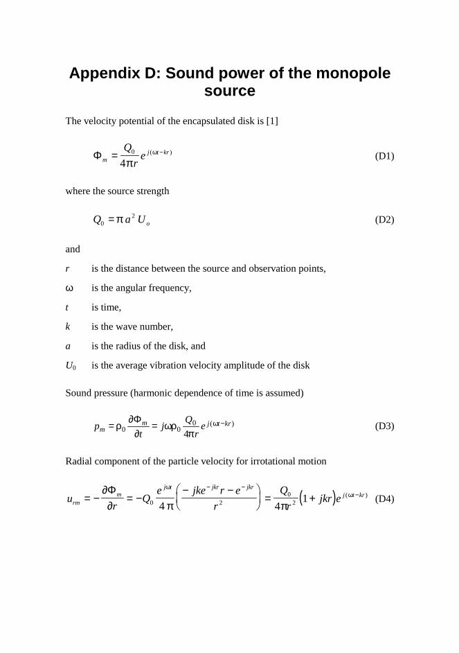
Appendix D: Sound power of the monopolesource

The velocity potential of the encapsulated disk is [1]

Φmj t krQ

re= −0

4πω( ) (D1)

where the source strength

Q a Uo02= π (D2)

and

r is the distance between the source and observation points,

ω is the angular frequency,

t is time,

k is the wave number,

a is the radius of the disk, and

U0 is the average vibration velocity amplitude of the disk

Sound pressure (harmonic dependence of time is assumed)

)(000 4

krtjmm e

rQj

tp −ω

πωρ=

∂Φ∂ρ= (D3)

Radial component of the particle velocity for irrotational motion

( )ur

Qe jke r e

rQ

rjkr erm

mj t jkr jkr

j t kr= − = −− −�

��

�

�� = +

− −−∂Φ

∂ π π

ωω

0 20

24 41 ( ) (D4)

D 2

Normal component of intensity

{ }I p u jQ

re

Qr

jkr e

jQ

rjkr k

Qr

rm m rmj t kr j t kr= = −

��

��

=��

�� −

��

��

=��

��

∗ − − −Re Re ( )

Re ( )

( ) ( )ωρπ π

ωρπ

ωρπ

ω ω0

0 02

00

2

3 00

2

4 41

41

14

(D5)

Sound power (integration of normal component of intensity over a sphere ofradius r)

( )

Π m rm

rm

r I d r kQ

rd k Q

k a Ua U

cU R

= =��

�� =

= = =

� �2 24

14

14 4

12

2

0

20

02

00 0

2

02

0

2 02 4

02

002

π θ θ π ωρπ

θ θπ

ωρ

πωρ π

πρ ω

π π

sin sin (D6)

The radiation resistance of the monopole source is

Ra

cc a karm = =

πρ ωρ π0

2 4

00 0

2 2

212

( ) (D7)

The pressure amplitude is inversely proportional to the distance r from the centreof the disk to the observation point, and the pressure disturbances at a certainpoint in the acoustic field are related to the amount of fluid being added orremoved by the actuator. The particle velocity is entirely radial, being in phasewith the pressure at distances that are large compared to the wavelength. Thetime-averaged intensity is also radial. The radiated sound power is proportionalto the square of the frequency.

Appendix E: Sound power of the dipolesource

The velocity potential of the free vibrating disk is [1] 1

( )Φd

jkrFc

er

J kaka

=�

��

�

��

−ω

ρ πθ

θθ

0 0

1

42 sin

sincos (E1)

where the net force exerted by the disk on adjacent fluid2

F a c U ka

a c j ka k a U ka

ω π ρ

π ρ

= >>

= + <<

2 1

32 1

20 0 0

20 0

4 40

1

( )(E2)

The factor in brackets of equation (E1) is the same as the one entering theexpression for the far field from a piston in a plane. In this case, however, thereis an extra directionality factor cosθ which ensures antisymmetry about thesymmetry plane. In low frequencies (for long wavelengths) the Bessel functionJ1(x) ≈ x/2 and the velocity potential becomes [2]

Φd

jkrFc

er

≈−

ω

ρ πθ

0 0 4cos (E3)

and [see also 3]

F j a Uω π ρ ω≈23

30 0 (E4)

Sound pressure (harmonic dependence of time is assumed)

pt

j Fc

er

jkFe

rdd

jkr jkr

= = =− −

ρ∂∂

ωρρ π

θπ

θωω0

0

0 0 4 4Φ

cos cos (E5)

1 The symbol j is used here instead of i. They are related so that i = -j and (i)2 = (j)2.2 The equation is incorrectly derived in reference [1] from equation 7.1.12.

E 2

Radial component of the particle velocity for irrotational motion

( )ur

Fc

jke r er

Fc

er

jkrrdd

jkr jkr jkr

= − = −− −�

��

�

�� = +

− − −∂∂

θπρ πρ

θω ωΦ coscos

4 41

0 02

0 02

(E6)

Intensity

{ }I p u jF

cjkr

rF

ckrrd d rd= =

�

��

�

��

−�

�

�

�

=

�

��

�

��

∗Re Recos cos

ωρθ

πρωρ

θπρ

ω ω0

0 0

2

3 00 0

2

241

4

(E7)

Sound power (integration of normal component of intensity over a sphere ofradius r)

Π d rr I dk F

cd= =

�

��

�

�� 2

82

0

0

0 0

2

2

0

π θ θωρ

π ρθ θ θ

πω

π

sin cos sin (E8)

By substitution x = cosθ, dx = -sinθdθ, x(0) = 1 and x(π) = -1

Π d

rd

k Fc

x dxk F

ck

ca U

a Uc

U R

=�

��

�

�� =

�

��

�

�� =

= =

−�

ωρπ ρ

ωρπ ρ πρ

π ρ ω

π ρ ω

ω ω0

0 0

2

2

1

10

0 0

22

0 0

2 602 2

02

04 6

02

03 0

2

8 12 1249

2712

(E9)

where the radiation resistance of the dipole source is

( )Ra

cc a kard = =

227

227

04 6

03 0 0

2 4π ρ ωρ π (E10)

E 3

The pressure amplitude is inversely proportional to the distance r from the centreof the disk to the observation point having its maximum along the dipole axis.The particle velocity is entirely radial, being in phase with the pressure atdistances large compared to the wavelength. The time-averaged intensity is alsoradial. The radiated sound power is more strongly dependent on the frequencythan the sound power of the monopole source.

Appendix F: The interaction of two dipolesources

When two dipole sources of the same phase are close to each other, according toFigure F1, the velocity potential is

�

�

� -

��

� � � � �

��

Figure F1. Two closely situated dipole sources.

( ) ( ) [ ]( ) ( )

Φdd

jkr jk r bjk r b j kb j kb

jk r b

Fc

er

er b

Fr c

e e e

Fr c

kb e

= ++

�

��

�

�� = +

=

− − +− + −

− +

ωθ

ω θ θ θ

ω θ

θπρ θ

θπ ρ

θπ ρ

θ

coscos

cos

coscos cos

coscos cos cos

cos

4 4

2

0 0 0 0

0 0

12

12

12

12

12

(F1)

The corresponding sound pressure and the normal component of the particlevelocity are, respectively

F 2

( ) ( )pt

jF k

rkb edd

dd jk r b= = − +ρ∂Φ

∂θ

πθω θ

0122

12

coscos cos cos (F2)

( ) ( )ur

Fr c

kb jkr

erdddd jk r b= − = +�

��

��

− +∂Φ∂

θπ ρ

θω θcoscos cos cos

21

0 0

12

12 (F3)

The intensity is the product of the sound pressure and the complex conjugate ofparticle velocity

[ ] ( ) ( )

( ) ( )

I p u jF k

r ckb jk

r

F k

r ckb

rdd dd rdd= = − +��

��

�

�

�

��

=

∗Re Recos

cos cos

coscos cos

ω

ω

θ

π ρθ

θ

π ρθ

2 2

20 0

2 12

2 2 2

20 0

2 12

21

2

(F4)

Integrating the normal component of the intensity over a sphere of radius rresults in the sound power the two dipole sources emits

( )( ) ( )Π dd rddr I d r

F k

r ckb d= = �� 2 2

22 2

2 2

20 0

2 2 12

00

π θ θ ππ ρ

θ θ θ θω

ππ

sin cos cos cos sin

(F5)

By substitution x = cosθ and dx = -sinθdθ, x(0) = 1 and x(π) = –1 then

( )Π dd

F kc

x kbx dx=−�

ω

πρ

2 2

0 0

2 2 121

1

2cos (F6)

Making use of the integral table [2]

( ) ( ) ( )x ax dx

x xa a

axx ax

a2 2

3 2

3 26 41

82

24� = + −

�

��

�

�� +cos sin

cos(F7)

F 3


k bkb= ⋅ ⋅ + −�

��

�� +

�

�

��6

13

11

2 22 2 2 2sin cos (F8)

If the two dipole sources are in opposite phases, the emitted sound power isaccordingly


k bkb− = ⋅ ⋅ − −�

��

�� −

�

�

��6

13

11

2 22 2 2 2sin cos (F9)

Appendix G: Dipole actuator locating on anabsorbent layer

The situation where the dipole source is located on an absorbent material isillustrated graphically in Figures G1 and G2. The absorbent material is locatedon an acoustically rigid layer. A mirror dipole source the phase of which isopposite compared to the real source is created on the other side of the layer.

� . � � � � � � � �

# ( � � ( � � �

# � � � � � � � � � � � � � � � � � � �

Figure G1. Dipole source on an absorbent layer.

�

�

� -

�

� � � � �

�

�

# � � � � � � � � � � � � � � � � � � �

Figure G2. Dipole source and its mirror dipole source.

G 2

By applying the image source principle, the velocity potential of the two dipolesources is

( )

( )[ ]

ΦΓ

Γ

Γ

Γ

ddhs

jkrjkr j

jkrjk r b j

jkr jk r b j

jkr

Fc

er r

e e

Fc

er r b

e e

Fr c

e e e

Fc

er

e

= −�

��

�

��

= −+

�

��

�

��

= −

= −

−− −

−− + −

− − + −

−

ω ς α ω

ω θ ς α ω

ω θ ς α ω

ω

θπρ

α ω

θπρ

α ωθ

θπ ρ

α ω

ρ πθ

cos ( , )'

cos ( , )cos

cos( , )

cos

' ( , )

cos ( , )

cos ( , )

4

4

4

41

0 0

0 0

0 0

0 0( ) ( )− − − −= −jkb j

djkb je e ecos cosθ ς θ ςΦ Γ1

(G1)

where

Τ(α,ω) is the reflection coefficient related to the absorbent surface

ς(α,ω) describes the phase between the incident and reflecting wave, and

α is the angle between the reflected wave and the normal to the planewhere the sources are located.

The corresponding sound pressure and the normal component of the particlevelocity are, respectively

( )

( )

pt

jF

ce

re e

p e e

ddhsddhs

jkrjkb j

djkb j

= = −

= −

−− −

− −

ρ∂Φ

∂ωρ

ρ πθω θ ς

θ ς

0 00 0 4

1

1

cos cos

cos

Γ

Γ(G2)

( )

( ) ( ) ( )

ur

Fc

e ejke r e

rF

cer

jkr e e u e e

rddhsddhs jkb j

jkr jkr

jkrjkb j

rdjkb j

= − = − −− −�

��

�

��

= + − = −

− −− −

−− − − −

∂Φ∂ πρ

θ

πρθ

ω θ ς

ω θ ς θ ς

41

41 1 1

0 02

0 02

cos

cos

cos

cos cos

Γ

Γ Γ

(G3)

The intensity is the product of sound pressure and complex conjugate of particlevelocity

G 3

[ ]

( ) ( )( )

( )( )[ ]

( )( )

( ))coscos(21

)coscos(214

cos

1Re14

cos

11114

cosRe

Re

2

22

0

220

2coscos3

2

00

coscos3

2

00

ς+θΓ−Γ+=

ς+θΓ−Γ+ρπ

θωρ=

Γ+Γ−Γ−+��

��

�

πρθ

ωρ=

��

�

�

�Γ−−Γ−��

�

��

�

πρθ

ωρ=

=

ω

ς−θ−ςθω

ςθς−θ−−ω

∗

kbI

kbcr

Fk

eeeejkrrc

F

eejkreeeerc

Fj

upI

r

jjkbjjkb

jjkbjkrjjkbjkr

rddhsddhsrddhs

(G4)

Integrating the normal component of the intensity over half sphere of radius rresults in the sound power the dipole sources emits

( )( )( )

( )( )�

�

�

πω

πω

π

θθθς+θΓ−Γ+π

ρω=

θθθς+θΓ−Γ+π

ρωπ=

θθπ=Π

2/

0

222

0

20

2/

0

222

0

202

2/

0

2

sincoscoscos218

sincoscoscos214

2

sin2

dkbZ

Fk

dkbZr

Fkr

dIr rddhsddhs

(G5)

By substitution x = cosθ and dx = -sinθdθ, x(0) = 1 and x(π/2) = 0 then

( )( )

( )( )dxkbxxxxZ

Fk

dxxkbxZ

Fkddhs

�

�

ς+Γ−Γ+π

ρω=

ς+Γ−Γ+π

ρω=Π

ω

ω

10

22222

0

20

10

222

0

20

cos28

cos218

(G6)

Making use of the integral table [2]

( ) ( ) ( )x ax dxx ax

aa x

aax2

2

2 2

3

2 2� = +

−cos

cossin (G7)

G 4

( ) ( ) ( )x ax dxx

aax

a xa

ax22

2 2

3

2 2� = −

−sin sin cos (G8)

( ) ( ) ( ) ( )( )

( ) ( )( )

( )( )

( )

( ) ( )( )

( )( )

( )

( ) ( )( )

( )( )

( )

( ) ( )( )

( )( )

( ) ( )( )

( ) ( )( ) ( )

( )

( ) ( )( ) ( )

( ) ( )( ) �

�

�

�ςΓ−��

�

�

��

�

��

�

�

��

�

−−ςΓ+

�

�

��

�

�

��

�

��

�

�

��

�

−+ςΓ−Γ+⋅Π⋅=

��

�ςΓ−��

�

�

��

�

−−ςΓ+

�

�

��

�

�

��

�

−+ςΓ−Γ+π

ωρ=

��

�

��

�

�

��

�

−−ςΓ+

�

�

��

�

�

��

�

−+ςΓ−Γ+π

ρω=

ςΓ+ςΓ−Γ+π

ρω=Π

ω

ω

ω

�

�

322

222

33

2

2

3

2

22

20

20

3

22

2

1

03

22

2323

20

20

10

222222

0

20

sin4cos211sin2sin2

sin211cos2cos2)1(31

23

sin4cos2sin2sin2

sin2cos2cos231

31

8

cos2sin2sin2

sin2cos2cos231

31

8

sinsin2coscos28

kbkb

kbkbkbkb

kbkbkbkb

kb

kbkb

kbkb

kbkb

kbkb

kbkb

kbZ

Fk

kbxkb

xkbkb

kbxx

kbxkb

xkbkb

kbxxxxZ

Fk

dxkbxxkbxxxxZ

Fk

d

ddhs

(G9)

If the reflecting surface is acoustically hard � Τ = 1 and ς = 0

( )( ) ( )

( )

( )( )

( )( )

Π Π

Π

ddhs d

d

kbkb kb kb

kb

kb kbkb

kbkb

= ⋅ ⋅ − + −�

��

�

��

�

��

�

��

�

��

= ⋅ ⋅ − −�

��

�

�� −

�

�

��

32

23

22 1

12

313

11

2 2

2 2

2 2

cossin

sin cos

(G10)

The result equals half of the sound power of two oppositely phased dipolesources which are located at a distance b from each other (Appendix E). If thedistance b between the sources approaches infinity, the radiated sound power isthe same as the radiated power of a single dipole source.

Appendix H: Radiation pattern of theactuator element

An EMFi actuator element is combined of several membrane strips which arelocated next to each other on the same plane. The different cells of the actuatorelement can be considered to operate as single line sources. The elementarysource is a part of a line source of length dx (see Figure H1)

/ � , &

� , &

�

�� -

� �

� �

�

� 0 � 1 � 1 � 2

Figure H1. Elementary source on the line source.

The source strength of an elementary source segment is

dQ U d dxm= 0 (H1)

H 2

where dm is the width of the line source and U0 is the radial vibration velocity.Each of the elementary source segments generates a pressure increment to thehalf space in the far field point (r, θ) (see Appendix D, equation D3)

dp jc kr

U d e dxmj t kr= −ρ

πω0 0

04 '( ') (H2)

The distance from the source point to the field point is r´ = r - xsinθ, r >> L (seeFigure H1). The resultant sound pressure is

p r t jc U kd

re e dx

jc U kL d

re

kLkL

jP r H e

m j t kr jkx

L

L

m j( t kr)

ax ej( t kr)

( , , )

sin( sin )sin

( ) ( )

( ) sin

/

/

θρ

π

ρπ

θθ

θ

ω θ

ω

ω

=

=�

��

�

��

=

−

−

−

−

�0 0 0

2

2

0 0 012

12

4

4(H3)

where

P rc U kL d

rH kLax

me( ) ( )

sinsin= = =

ρπ

θν

νν θ0 0 0 1

24 and where

(H4)

The function He(θ) is the zeroth order spherical Bessel function of the first kind,jo(ν). An EMFi actuator is built of N adjacent strip elements which are separatedby a distance dm from each other. They have the same source strength and theyradiate with the same phase according to Figure H2.

H 3

�

� �

� 0 � 1 � 1 � 2

� � - � & -

�

� �

Figure H2. The line source elements.

In the acoustic far field all the rays from the array of line sources to the fieldpoint can be considered parallel (see Figure H2). Source i produces soundpressure

p r t jc U kL d

rH ei

m

i

j( t kr')i( , , )'

( )Φ = −ρπ

θ ω0 0 0

4(H5)

The resultant pressure at the field point is the summation

p r t jc U kLd

He

rTOTm

j( t kr')

ii

N i

( , , ) ( )'

Φ =−

=�

ρπ

θω

0 0 0

14(H6)

The distance between the element source and the field point is ri’ = r1 - (i-1)∆rwhere ∆r = dm sinφ. The distance to the centre of the array of line sources is r =r1 - ½ P/dm ∆r where the length of the array is P = (N-1) dm.

H 4

p r t jc U kLd

rH e e eTOT

m jP

dk r

j t kr j i k r

i

Nm( , , ) ( ) ( ) ( )Φ

∆∆=

−− −

=�

ρπ

θ ω0 0 012 1

14(H7)

( ) ( )[ ]( ) ( )

( )( ) ( )

( )( )

( )( )

( )

e e ik r j ik r

k r k rj

k r k r

k re

k re

j i k r

i

Njik r

i

N

i

N

N N

k r

N N

k r

N

k rj k r

N

k r

jP

dk rN

m

( )

( )

cos sin

sin cossin

sin sinsin

sinsin

sinsin

−

= =

−

=

−

− −

� � �= = +

= +

= =−

1

1 0

1

0

1

21

2

2

21

2

2

2

2

2

2

121

2

∆ ∆

∆ ∆

∆∆

∆

∆

∆ ∆

∆ ∆ ∆ ∆

∆ ∆

( )( )( )( )

p r t jc U kLd

rH

k rk r

e

jc U kLd

rH

kdkd

e

jP H H e

TOTm

e

Nj( t kr)

me

Nm

m

j( t kr)

ax ej( t kr)

( , , ) ( )sinsin

( )sin sinsin sin

( ) ( )

Φ∆∆

=

=

=

−

−

−

ρπ

θ

ρπ

θφφ

θ φ

ω

ω

ω

0 0 0 212

0 0 0 2

12

4

4(H8)

where ( )( )φ

φ=Φ

sinsinsinsin

)(212

m

mN

kdkd

H

Appendix I: Sound power of natural modeof a simply supported plate

Surface velocity distribution of a (m,n) mode of a simply supported plate with aninfinite baffle is [4]

u um x

an y

bmωπ π

= ��

��

��

��sin sin (I1)

where 0 0≤ ≤ ≤ ≤x a y b ;

� �

�

�

�

�

�

�

��

� 0 � 1 � �2

Figure I1. Simply supported plate with infinite baffle.

I 2

Sound pressure in the acoustic far field according to Rayleigh integral is [3]

p jk ce

ru x y e e dxdy

jk ce

ru

m xa

n yb

e e dxdy

jkrj x j y

a

a

b

b

jkr

mj x j y

a

a

b

b

a b

a b

ω ωρπ

ρπ

π π

α β

α β

=

= ��

��

−

−−

−

−−

��

��

0 0 2

2

2

2

0 0 2

2

2

2

2

2

( , )

sin( ) sin

/

/

/

/

/

/

/

/(I2)

where α θ φ β θ φ= =ka kbsin cos sin sin and

By integration

( )[ ]sin

m xa

e dx

am

e

m

a ja

x

m j

π παπ

αα

��

�� =

− −

��

�� −

�0 2

1 1

1

( )[ ]sin

n yb

e dy

bn

e

n

b jb

y

n j

π πβπ

ββ

��

�� =

− −

��

�� −

�0 2

1 1

1

Sound pressure in the acoustic far field is

( ) ( )p ju k c

er

abmn

e

m

e

n

m

-jkr m j n j

ω

α β

ρπ π α

πβπ

=− −��

�� −

�

�

�

��

− −��

�� −

�

�

�

��

0 0 2 2 221 1

1

1 1

1 (I3)

The average sound power on the one side of the plate radiates to the acoustic farfield

Π sspmp

cr d d c

u kabmn

m n

d d= =�

��

�

��

��

��

�

��

�

��

��

�� −

�

�

��

��

�

�� −

�

�

��

�

�

�

��

⋅�� ω

π π

ρθ θ φ ρ

π

α β

απ

βπ

θ θ φ

π π2

0 000

22

0 0 3

2

2 200

2

2

2 2

42 2

1 1sin

cossin

cossin

sin

(I4)

The odd modes of the equation (I4) are related to the cosine terms and the evenmodes correspondingly to the sinus terms.

Appendix J: Sound power of natural modeof a rigidly supported plate

Surface velocity distribution of mode (m,n) of a rigidly supported plate with aninfinite baffle is [5]

( )( )

( )( )

( )( )

( )( )u u

k xk a

k xk a

k y

k b

k y

k bm

xm

xm

xm

xm

yn

yn

yn

ynω = −

�

��

�

�� −�

�

��

�

�

��

cosh

cosh ½

cos

cos ½

cosh

cosh ½

cos

cos ½(J1)

where− ≤ ≤ − ≤ ≤ = =a x a b y b k m a k n bxm yn/ / / / / /2 2 2 2 ; ; ; π π

�

�

�

�

�

�

� 0 � 1 � �

��

�

�

Figure J1. Rigidly supported plate with infinite baffle.

J 2

Sound pressure in the acoustic far field according to Rayleigh integral is [3]

( )( )

( )( )

( )( )

( )( )

p jk ce

ru x y e e dxdy

jk c ue

rk xk a

k xk a

k y

k b

k y

k be e dxdy

jkrj x j y

a

a

b

b

m

jkrxm

xm

xm

xma

a

b

b

yn

yn

yn

yn

j x j y

a b

a b

ω ωρπ

ρπ

α β

α β

=

= −�

��

�

��

⋅ −�

�

��

�

�

��

−

−−

−

−−

��

��

0 0 2

2

2

2

0 0 2

2

2

2

2

2

( , )

coshcosh ½

coscos ½

cosh

cosh ½

cos

cos ½

/

/

/

/

/

/

/

/(J2)

where α θ φ β θ φ= =ka kbsin cos sin sin and

By integration

( ) ( )[ ] ( ) ( )[ ]cosh( ) sinh ½ sinh ½/

/k x e dx

k j

kk a j

k j

kk a jxm

j x

a

a xm a

xm axm

xm a

xm axm

aα

α

α

α

αα α

−� =−

++ +

+

+−

2

2

2 2 2 2

where ( )[ ]sinh ½ sinh cos cosh sink a jk a

jk a

xmxm xm+ =

�

��

�

��

��

�� +

�

��

�

��

��

��α

α α2 2 2 2

Thus the integral above is

( ) ( )

( )

( )

cosh sinh cos cosh sin

sinh cos cosh sin

/

/k x e dx

k j

k

k aj

k a

k j

k

k aj

k a

k

xma

a ja

x xm a

xm a

xm xm

xm a

xm a

xm xm

xm a

−� =−

+�

��

�

��

��

�� + �

��

�

��

��

��

�

�

�� +

+

+�

��

�

��

��

�� − �

��

�

��

��

��

�

�

��

=+

2

2

2 2

2 2

2 2

2 2 2 2

2 2 2 2

2

α α

α

α

α

α

α α

α α

kk a

ak a

xmxm xmsinh cos cosh sin2 2 2 2

�

��

�

��

��

�� + �

��

�

��

��

��

�

�

��

α α α

J 3

Correspondingly, the other integrals are

( ) ( )cosh sinh cos cosh sin

/

/k y e dy

kk

k bb

k bynb

b jb

y

yn b

ynyn yn

−� =+

�

��

�

��

��

�� +

�

��

�

��

��

��

�

�

��2

2

2 2

22 2 2 2

β

β

β β β

( )coscos sin

/

/k x e dx

akk a

ak

xma

a ja

y xm

xm

xm

−� =

− �

��

�

��

��

��

−�

��

�

��

2

22

2

22 2

1

α

α α

α

( )coscos sin

/

/k y e dy

bkk b

bk

ynb

b jb

y yn

yn

yn

−� =

− �

��

�

��

��

��

−�

��

�

��

2

22

2

22 2

1

β

β β

β

The sound pressure is

p jk c ue

rk

a

kk a

a

ak

akk

b

kk b

m

jkr

xm

xmxm

xm

xmyn

ynyn

ω ρπ α

α α α

α

α αβ

=+ ��

��

�

��

�

��

��

�� + �

��

��

�

��

�

��

�

�

�

��

��

+

−�

��

�

��

��

��

�

��

�

��

�

�

��

⋅+ ��

��

�

��

�

�

−

0 02

2

2 22

2

22

2 2 2

1

1

22

22

tanh cos sin

sin tanh ��

�� + �

��

��

�

��

�

��

�

�

+

−�

��

�

��

��

��

�

��

�

��

�

�

��

�

�

��

�

��

cos sin

sin

β β β

β

β β

2 2

1

1

222 2

b

bk

bk

yn

yn

(J3)

J 4

The average sound power radiating on one side of the plate to the acoustic farfield is

Π rspm

xm

xmxm

xm

xm

pc

r d d cu k

ka

kk a

a

akak

= = ��

��

+ ��

��

⋅

�

�

��

��

��

��

�

��

+ ��

��

��+

−�

��

�

��

��

��

�

��

�

��

�

��

�� ω

π π

ρθ θ φ ρ

π αα

α α

α

α α

π π2

0 000

22

0 0

2

22

00

2

2 2

2 2

41

2 2

21

12

sin tanh cos

sin sin ⋅+ ��

��

�

�

�

��

�

��

��

��

�

��

+ ��

��

��+

−�

��

�

��

��

��

�

��

�

��

�

��

12 2

21

12

22

2 2

2

kb

kk b

b

bk

bkd d

yn

ynyn

yn

yn

ββ

β β

β

β βθ θ φ

tanh cos

sin sin sin

(J4)

Appendix K: Inequality condition for acombined standard deviation

From equations (45) and (46) the inequality condition uc1(y) ≤ uc2(y) reduces toequation

( )( ) ( )10 1010 2

1

10

1

x a

i

Nx a

i

Ni i i i+

=

+

=� �≤/ / (K1)

Because

( )( ) ( ) ( )10 10 1010 2

1

10

1

210

1

x a

i

Nx a

i

Nx a

i

Ni i i i i i+

=

+

=

+

=� � �≤

�

��

�

�� =/ / / (K2)

the condition is valid. In a similar way it is possible to show for equations (47),(48) and (49), (50) that uc1(y) ≤ uc2(y).

References for Appendices

1. Morse, P. M. and Ingard, K. U. Theoretical Acoustics. New York - St.Louis - San Francisco - Toronto - London - Sydney: McGraw-Hill, 1968.927 p.

2. Abramowitch, M. and Stegun, I. A. Handbook of mathematical functions.New York: Dover publications, 1970. 1046 p.

3. Pierce, A. D. Acoustics. An introduction to its physical principles andapplications. New York: McGraw-Hill, 1991. 678 p.

4. Skudrzyk, E. The foundations of acoustics. Wien - New York: SpringlerVerlag, 1971. 790 p.

5. Malecki, I. Physical foundations of technical acoustics. Oxford - London -Edinburgh - New York - Toronto - Sidney - Paris - Braunschweig:Pergamon Press, 1969. 743 p.

Published by

Vuorimiehentie 5, P.O.Box 2000, FIN-02044 VTT, FinlandPhone internat. +358 9 4561Fax +358 9 456 4374

Series title, number andreport code of publication

VTT Publications 405VTT–PUBS–405

Author(s)Saarinen, Ari

Title

EMFi-actuator: vibro-acoustical considerationAbstract

In this paper the vibro-acoustical properties of the EMFi-actuator are studied. The examination is carried out by modelling the operation ofthe actuator and by comparing the modelling results to the corresponding measured values in case they are available. The modelling isbased on an analytical approach. The equations used are derived in the Appendices. Consideration on the properties of the vibration isdivided into three parts: the basic vibration of the film, vibration of the film in the time domain and vibration of the functional elements ofthe actuator. The sound production properties of the actuator have been examined in the free acoustic field and in cases with boundariesnear the source. The effect of the different vibration distributions of the actuator film and impedance loading for the emitted sound hasbeen studied. Also the radiation pattern of the actuator is modelled and compared to the measured results.The general vibro-acoustical functioning of the EMFi-actuator is stated in the impedance-oriented form by evaluating the loadingimpedance of the vibrating film from its boundary conditions. The basic vibration functioning of the actuator film in the frequency domainis predicted by using a linear second-order ordinary differential equation with constant coefficients. In the time domain the non-lineareffects of the spring force and electric forces acting on the actuator film are considered. The recoil effect of the actuator is studied with anormal-mode method of dynamic analysis. It is found that the response of the supporting structure may decrease with about a decadewithout influencing the response of the actuator film.The use of the arithmetic average value of the vibration deflection of the EMFi-actuator in the prediction of sound power or soundpressure in the acoustic far field at low frequencies is compared to the frequency or spatially dependent vibration of the actuator film. Thevalue of the arithmetic average of vibration is valid even when the outward impedance of the film is not taken into consideration. Thelarge dipole type actuators are more effective sound radiators than monopole sources. The effect of the thickness of the absorbent materialunder the dipole actuator, the radiation pattern and the effect of the boundary conditions of the vibrating cell on the radiating sound powerare considered. The measured and predicted values of radiation patterns are very similar in every angle. The rigidly supported boundary ofthe actuator cell enables the actuator panel to radiate much more sound power with all the different even modes than it is possible with asimply supported boundary condition. The basic problems concerning the operation of an EMFi-actuator are related to its ineffective lowfrequency sound production and the distortion caused by non-linear vibration. It is possible to increase the sound power radiationproperties of the monopole or dipole type functional modes of the actuator by making the deflection of the membrane larger (using smallertension), by using larger membrane areas or by using two interacting actuators. The dimensions of the actuator element cell affect thepower the single vibration mode is able to radiate into the acoustic far field. When the film cells of the actuator panels are simplysupported, the larger dimensions compared to those of the present actuator type, produce more sound power at odd and even modes.The confidence intervals of a normal distribution used in the evaluation of the reliability of the sound power measurements have beenobtained by calculating combined standard deviation values from standard deviation values of single frequency bands given in thestandards. It is shown that it is possible to find an upper limit for the confidence interval.The main results of this work are the means to increase the radiated sound power of the actuator element without increasing concurrentlythe distortion of the radiator. These resources are based on the functioning mode of the actuator (monopole, dipole), boundary conditionsof the actuator element or cells of the actuator element, the larger actuator areas, interaction of actuators and the dimensions of theactuator element cells. Another result of this study is the potentiality to evaluate the A-weighted standard deviation of the sound power ofthe equipment to be measured from the measurement results without specifying the type of emitted sound radiated by the equipment.

KeywordsEMFi-actuator, actuators, vibration, acoustic properties, modelling, evaluation, vibro-acoustical properties,sound production, measurement

Activity unitVTT Building Technology, Building Physics, Building Services and Fire Technology,Lämpömiehenkuja 3, P.O.Box 1804, FIN–02044 VTT, Finland

ISBN Project number951–38–5554–6 (soft back ed.)951–38–5555–4 (URL: http://www.inf.vtt.fi/pdf/)

R9SU00394

Date Language Pages PriceDecember 1999 English 109 p. + app. 30 p. C

Name of project Commissioned byACTIVA, FACTS Tekes, EU

Series title and ISSN Sold byVTT Publications1235–0621 (soft back ed.)1455–0849 (URL: http://www.inf.vtt.fi/pdf/)

VTT Information ServiceP.O.Box 2000, FIN-02044 VTT, FinlandPhone internat. +358 9 456 4404Fax +358 9 456 4374

vibro-acoustical consideration emfi-actuator

Documents