Hole Filling in Images

Siddharth Jain

Video and Image Processing Laboratory

Submitted to the Department of Electrical Engineering and Computer Sciences, University of Cal-

ifornia at Berkeley, in partial satisfaction of the requirements for the degree of Master of Science,

Plan II.

Approval for the Report and Comprehensive Examination:

Committee:

Professor Avideh Zakhor

Research Advisor

Date

* * * * * *

Professor David Forsyth

Second Reader

Date

Abstract

This project relates to automated 3D model generation of Urban Environments. Ground based

modeling involves a setup of two 2D laser scanners, and a digital camera mounted on top of a

truck. As we drive the truck in a city, the laser scans capture depth information using the LIDAR

time-of-flight principle. These laser scans are then subjected to accurate localization and 3D data

processing algorithms to create a 3D mesh of the urban environment. The resulting mesh is then

texture mapped with camera images to produce photo-realistic models.

In doing so, foreground objects such as trees, cars, lamposts etc. occlude parts of the back-

ground buildings from the laser scanners and the digital camera, and thus leave holes both in the

geometry and texture. For a 3D model, ideally the user should be able to view the building facade

that is occluded by a tree or other objects.

In this report, we present a simple and efficient method for filling holes in images obtained

through the above setup. Given an image with regions of unknown RGB values, our goal is to

determine the missing pixel values from the remainder of the image. We use our proposed method

to fill holes in the texture atlases generated during automated 3D modeling of Urban Environ-

ments. Our approach can also be used for other applications such as restoring old and damaged

photographs, removing objects from images, special effects.

Our method first fills low pixel variance regions by a pass of 1D horizontal interpolation in

which for each row it linearly interpolates any missing values, if they lie in a low pixel variance

region. This is followed by a pass of 1D vertical interpolation. A copy-paste method is then

employed to synthesize the missing texture. A window is taken around the hole, and a matching

region in the image is found. The hole is filled by copying the matching region and pasting it over

the hole.

The approach is found to work well on most images and does not suffer from the limitations of

local inpainting in traditional hole filling schemes.

Contents

1 Introduction 2

1.1 Existing approaches and previous work . . . . . . . . . . . . . . . . . . . . . . . 6

1.2 Salient features of our images . . . . . . . . . . . . . . . . . . . . . . . . . . . . . 7

2 Texture Atlas Generation 9

2.1 Foreground and Background Segmentation of Images . . . . . . . . . . . . . . . . 9

2.1.1 Correspondence Error . . . . . . . . . . . . . . . . . . . . . . . . . . . . 14

2.2 Texture Atlas Generation . . . . . . . . . . . . . . . . . . . . . . . . . . . . . . . 18

3 Hole Filling of the Atlases 22

3.1 Horizontal and Vertical Interpolation . . . . . . . . . . . . . . . . . . . . . . . . . 22

3.2 The Copy-Paste Method . . . . . . . . . . . . . . . . . . . . . . . . . . . . . . . 24

4 Results and Remarks 29

1

Chapter 1

Introduction

At the Video and Image Processing Laboratory (VIP Lab), University of California Berkeley we

are engaged in automated 3D model generation of Urban Environments. This has important appli-

cations in virtual reality, gaming and generating special effects for movies.

Camera and laser scanners are by far the most common devices used for 3D model reconstruc-

tion. Far range modeling from an airplane utilizes airborne laser scans and aerial images to create

models appropriate for virtual fly-throughs. For virtual drive-throughs and walk-throughs we need

a more photorealistic and detailed model which can be acquired through ground based modeling.

An innovative image based reconstruction approach to automated model acquisition in urban areas

has been developed at the MIT City Scanning Project [Tel98, AT00] in which a large number of

images are mosaiced into a super high resolution spherical image, enabling accurate extraction of

features, vanishing lines and pose estimation. However, the acquisition speed is limited since the

data has to be collected in a slow stop-and-go fashion resulting in several days acquisition time for

an entire city. Stamos and Allen [SA00] describe a method for acquiring building facades with a

mobile robot equipped with Cyrax 3D laser scanner and a camera. Their approach, though auto-

matic, is time consuming due to the slow 3D scanner. The acquisition time for a single building

is already more than an hour. Although 3D scanners provide more information than 2D scanners,

they are significantly slower than 2D scanners. Thrun et. al. [TBF00] and Hahnel et. al. [HBT01]

use 2D laser scanners for mobile robotic applications to learn 3D models of indoor and outdoor

environments. Zhao and Shibasaki [ZS99] describe a system consisting of 2D scanners and digital

2

camera mounted on a car that can be efficiently used for modeling cities. Their localization unit

consists of a Global Positioning System (GPS) and odometry sensors to determine the vehicle’s

position during data acquisition.

Fruh and Zakhor [FZ01a] recently proposed a novel method for rapid acquisition and construc-

tion of 3D models of cities. The data acquisition system is shown in Fig. 1.1, and involves a setup

of two 2D laser scanners and a digital camera all synchronized with each other and mounted on

top of a truck. As the truck is driven in a city, the vertical laser scans capture depth information

using the LIDAR time-of-flight principle. The pose of the vehicle is accurately determined by

matching the horizontal laser scans, and using information from digital roadmaps and aerial pho-

tographs [FZ01b]. The vertical scans are then stacked together and subjected to 3D data processing

algorithms to create a 3D mesh of the urban environment. The resulting mesh is texture mapped

with camera images to produce photo-realistic models [FZ02].

Fig. 1.2 shows a 3D point cloud containing vertices for all objects in the scanner’s field of view.

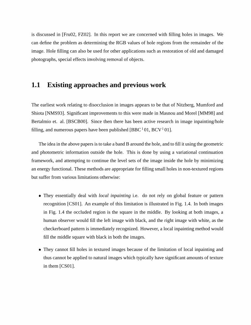
Fig. 1.3(a) shows the raw mesh obtained after triangulation of this 3D point cloud. Objects such as

trees, overhead transmission wires, glass and windows pose special problems with laser scans. The

laser beam is scattered by the trees, and does not have enough resolution to capture the overhead

transmission wires accurately. When the beam encounters glass, most of the energy is transmitted,

and then scattered by objects such as walls. In the raw mesh the overhead wires appear as bits

floating in the sky, and the trees and windows are also not properly reconstructed. These problems

are further discussed in [Fru02, FZ02].

The triangulated raw mesh appears especially problematic when viewed from the side as in

Fig. 1.3(b). To remedy this, the raw mesh is separated into two layers — the background containing

the building facades which have to be accurately reconstructed, and the foreground containing

trees, overhead wires, lamp posts, bins, etc. The foreground objects, however, occlude parts of the

background layer. The laser scans and the camera images cannot capture the part of a building

facade that is hidden behind a foreground object. These regions where the geometry and texture

of the background layer are missing are called holes. In order to provide a complete 3D model

in which the user can view the facade from an arbitrary vantage point, we need to fill the missing

geometry and texture in the holes. This is critical in our current setup in which the foreground layer

is actually removed from the 3D model [FZ02] and the holes are exposed. Hole filling in the mesh

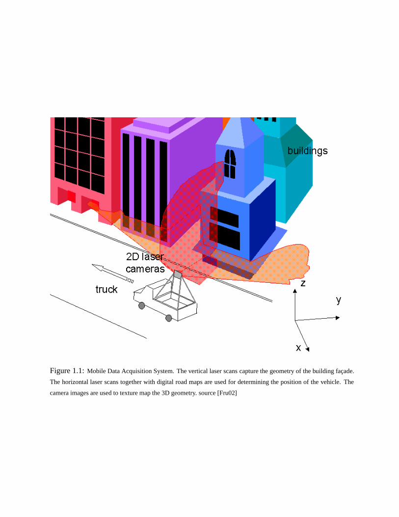
Figure 1.1: Mobile Data Acquisition System. The vertical laser scans capture the geometry of the building facade.

The horizontal laser scans together with digital road maps are used for determining the position of the vehicle. The

camera images are used to texture map the 3D geometry. source [Fru02]

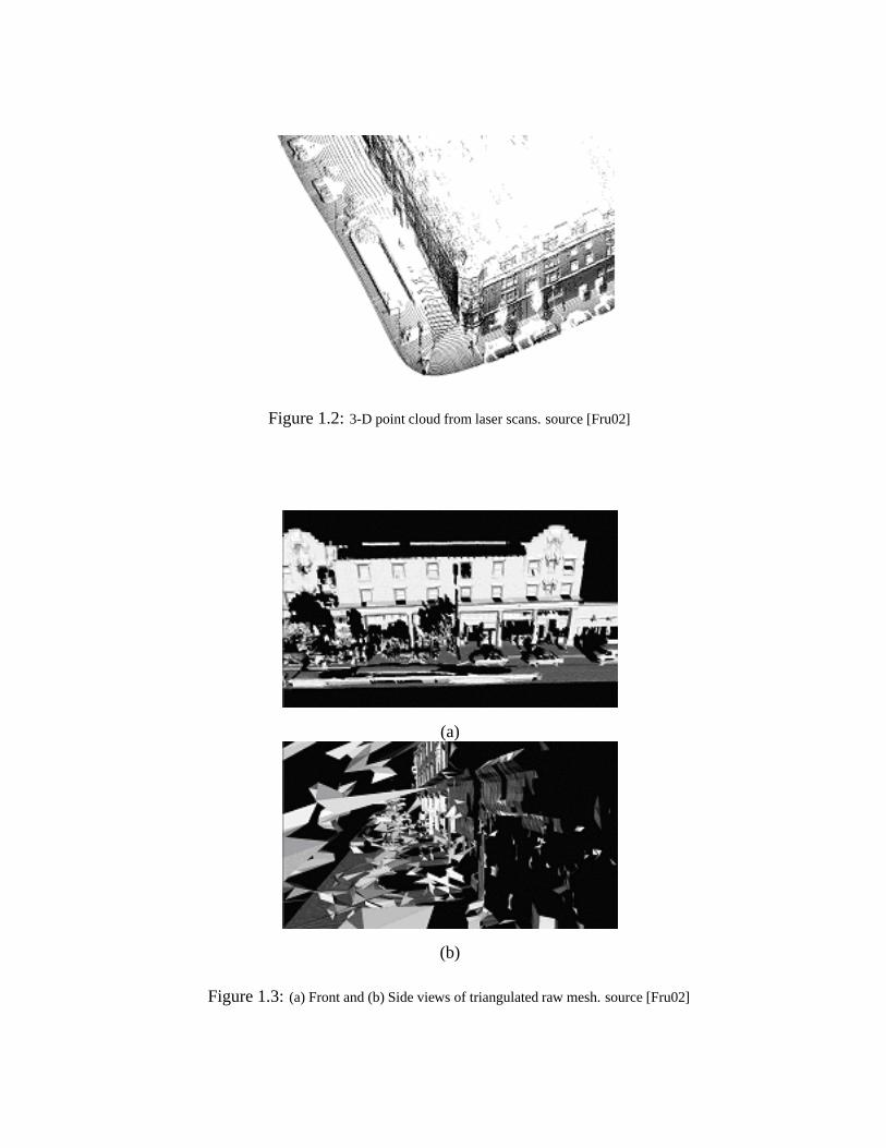
Figure 1.2: 3-D point cloud from laser scans. source [Fru02]

(a)

(b)

Figure 1.3: (a) Front and (b) Side views of triangulated raw mesh. source [Fru02]

is discussed in [Fru02, FZ02]. In this report we are concerned with filling holes in images. We

can define the problem as determining the RGB values of hole regions from the remainder of the

image. Hole filling can also be used for other applications such as restoration of old and damaged

photographs, special effects involving removal of objects.

1.1 Existing approaches and previous work

The earliest work relating to disocclusion in images appears to be that of Nitzberg, Mumford and

Shiota [NMS93]. Significant improvements to this were made in Masnou and Morel [MM98] and

Bertalmio et. al. [BSCB00]. Since then there has been active research in image inpainting/hole

filling, and numerous papers have been published [BBC�01, BCV�01].

The idea in the above papers is to take a band B around the hole, and to fill it using the geometric

and photometric information outside the hole. This is done by using a variational continuation

framework, and attempting to continue the level sets of the image inside the hole by minimizing

an energy functional. These methods are appropriate for filling small holes in non-textured regions

but suffer from various limitations otherwise:

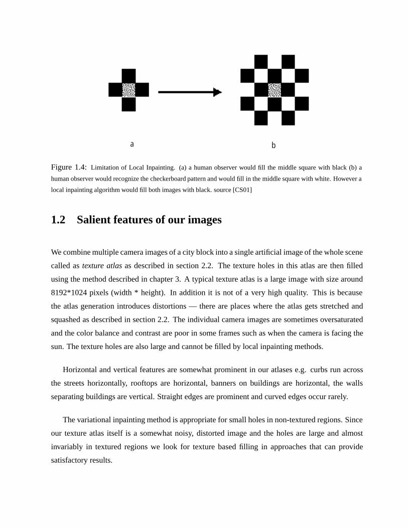
� They essentially deal with local inpainting i.e. do not rely on global feature or pattern

recognition [CS01]. An example of this limitation is illustrated in Fig. 1.4. In both images

in Fig. 1.4 the occluded region is the square in the middle. By looking at both images, a

human observer would fill the left image with black, and the right image with white, as the

checkerboard pattern is immediately recognized. However, a local inpainting method would

fill the middle square with black in both the images.

� They cannot fill holes in textured images because of the limitation of local inpainting and

thus cannot be applied to natural images which typically have significant amounts of texture

in them [CS01].

a� b�

Figure 1.4: Limitation of Local Inpainting. (a) a human observer would fill the middle square with black (b) a

human observer would recognize the checkerboard pattern and would fill in the middle square with white. However a

local inpainting algorithm would fill both images with black. source [CS01]

1.2 Salient features of our images

We combine multiple camera images of a city block into a single artificial image of the whole scene

called as texture atlas as described in section 2.2. The texture holes in this atlas are then filled

using the method described in chapter 3. A typical texture atlas is a large image with size around

8192*1024 pixels (width * height). In addition it is not of a very high quality. This is because

the atlas generation introduces distortions — there are places where the atlas gets stretched and

squashed as described in section 2.2. The individual camera images are sometimes oversaturated

and the color balance and contrast are poor in some frames such as when the camera is facing the

sun. The texture holes are also large and cannot be filled by local inpainting methods.

Horizontal and vertical features are somewhat prominent in our atlases e.g. curbs run across

the streets horizontally, rooftops are horizontal, banners on buildings are horizontal, the walls

separating buildings are vertical. Straight edges are prominent and curved edges occur rarely.

The variational inpainting method is appropriate for small holes in non-textured regions. Since

our texture atlas itself is a somewhat noisy, distorted image and the holes are large and almost

invariably in textured regions we look for texture based filling in approaches that can provide

satisfactory results.

Although we have developed our method taking into consideration these special features, we

have applied it to other images, with results comparable to those published in above cited papers.

Another important consideration in our work is that it is fully automated. We use a single set of

parameters to process all the images.

This report is organized as follows: Chapter 2 discusses the atlas generation process. This

involves segmenting out the foreground in individual camera images followed by combining mul-

tiple images into a single texture atlas. Chapter 3 discusses hole filling in the texture atlas. Finally,

results and remarks are discussed in chapter 4.

Chapter 2

Texture Atlas Generation

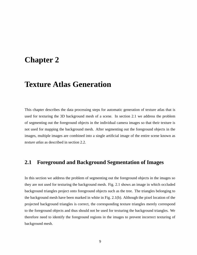
This chapter describes the data processing steps for automatic generation of texture atlas that is

used for texturing the 3D background mesh of a scene. In section 2.1 we address the problem

of segmenting out the foreground objects in the individual camera images so that their texture is

not used for mapping the background mesh. After segmenting out the foreground objects in the

images, multiple images are combined into a single artificial image of the entire scene known as

texture atlas as described in section 2.2.

2.1 Foreground and Background Segmentation of Images

In this section we address the problem of segmenting out the foreground objects in the images so

they are not used for texturing the background mesh. Fig. 2.1 shows an image in which occluded

background triangles project onto foreground objects such as the tree. The triangles belonging to

the background mesh have been marked in white in Fig. 2.1(b). Although the pixel location of the

projected background triangles is correct, the corresponding texture triangles merely correspond

to the foreground objects and thus should not be used for texturing the background triangles. We

therefore need to identify the foreground regions in the images to prevent incorrect texturing of

background mesh.

9

(a)

(b)

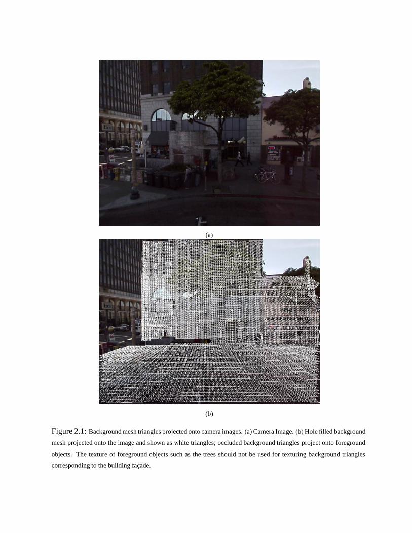
Figure 2.1: Background mesh triangles projected onto camera images. (a) Camera Image. (b) Hole filled background

mesh projected onto the image and shown as white triangles; occluded background triangles project onto foreground

objects. The texture of foreground objects such as the trees should not be used for texturing background triangles

corresponding to the building facade.

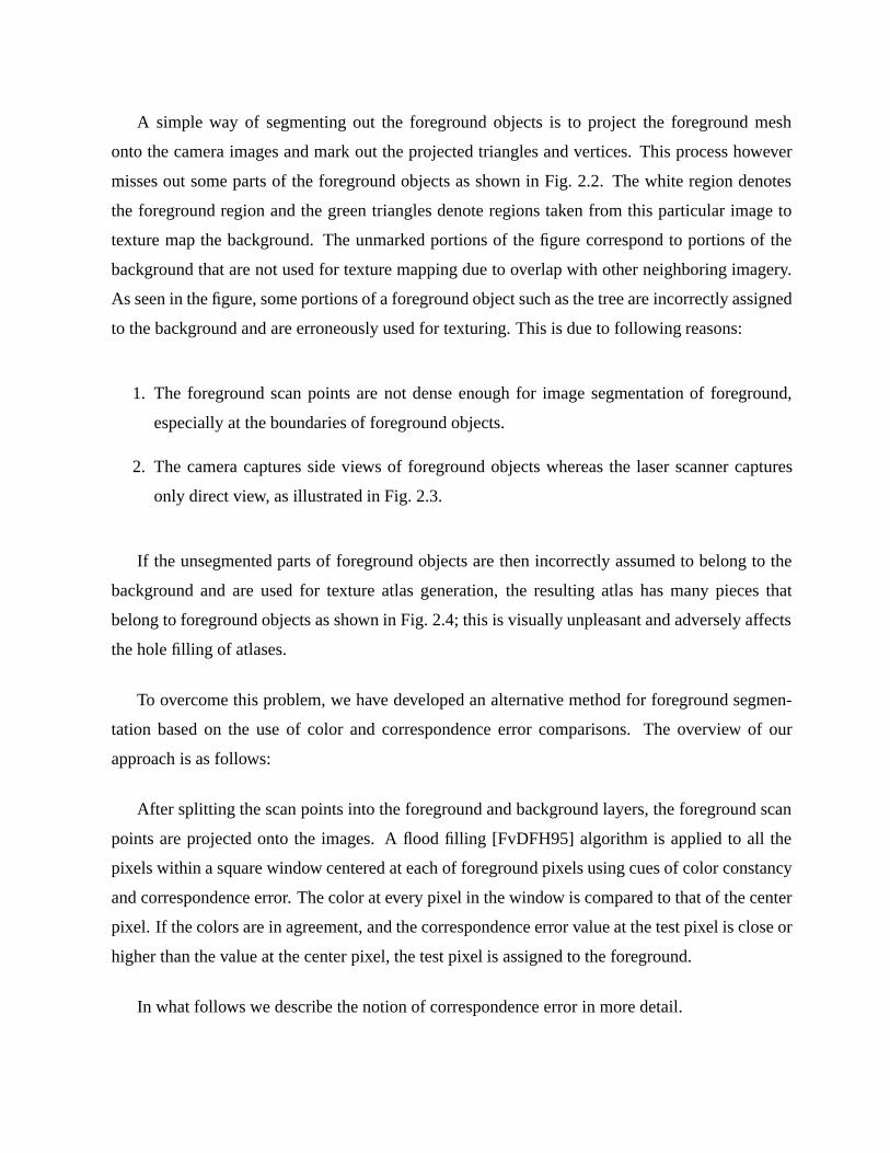
A simple way of segmenting out the foreground objects is to project the foreground mesh

onto the camera images and mark out the projected triangles and vertices. This process however

misses out some parts of the foreground objects as shown in Fig. 2.2. The white region denotes

the foreground region and the green triangles denote regions taken from this particular image to

texture map the background. The unmarked portions of the figure correspond to portions of the

background that are not used for texture mapping due to overlap with other neighboring imagery.

As seen in the figure, some portions of a foreground object such as the tree are incorrectly assigned

to the background and are erroneously used for texturing. This is due to following reasons:

1. The foreground scan points are not dense enough for image segmentation of foreground,

especially at the boundaries of foreground objects.

2. The camera captures side views of foreground objects whereas the laser scanner captures

only direct view, as illustrated in Fig. 2.3.

If the unsegmented parts of foreground objects are then incorrectly assumed to belong to the

background and are used for texture atlas generation, the resulting atlas has many pieces that

belong to foreground objects as shown in Fig. 2.4; this is visually unpleasant and adversely affects

the hole filling of atlases.

To overcome this problem, we have developed an alternative method for foreground segmen-

tation based on the use of color and correspondence error comparisons. The overview of our

approach is as follows:

After splitting the scan points into the foreground and background layers, the foreground scan

points are projected onto the images. A flood filling [FvDFH95] algorithm is applied to all the

pixels within a square window centered at each of foreground pixels using cues of color constancy

and correspondence error. The color at every pixel in the window is compared to that of the center

pixel. If the colors are in agreement, and the correspondence error value at the test pixel is close or

higher than the value at the center pixel, the test pixel is assigned to the foreground.

In what follows we describe the notion of correspondence error in more detail.

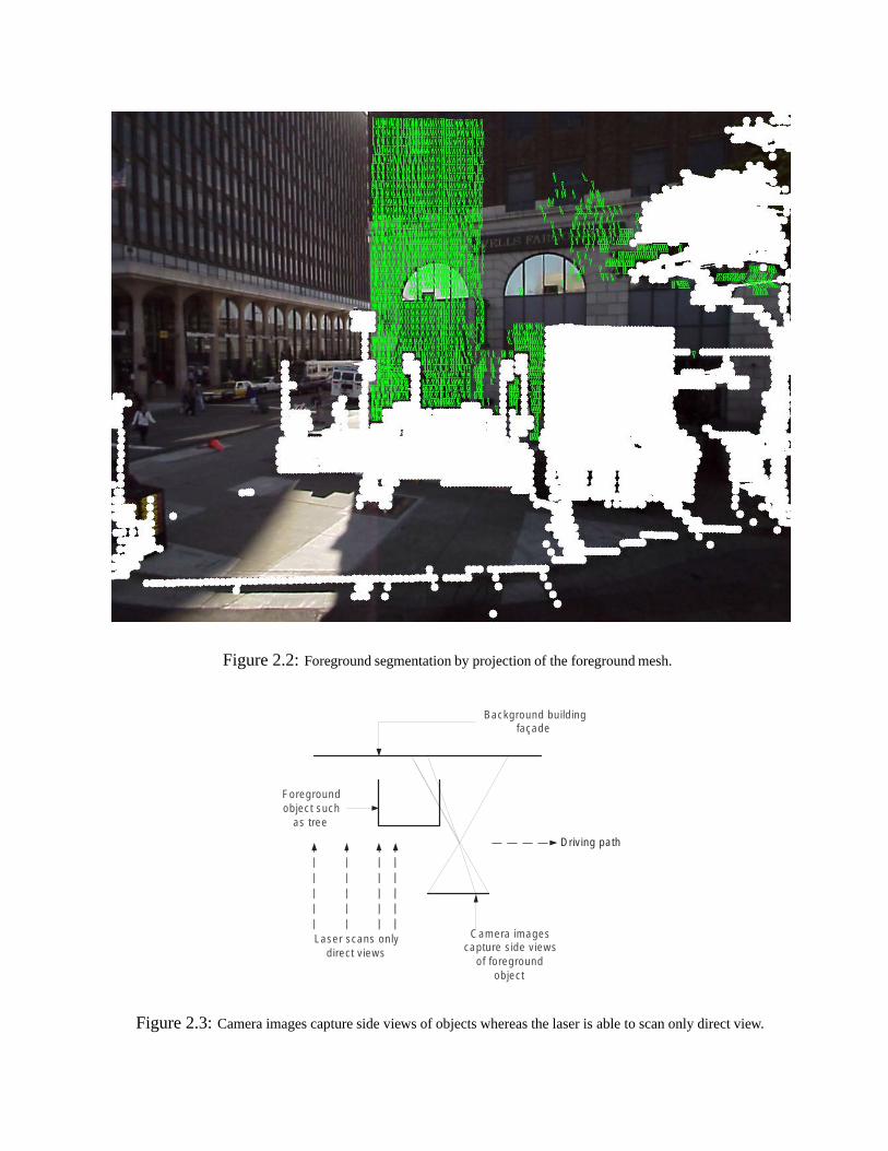
Figure 2.2: Foreground segmentation by projection of the foreground mesh.

Driving path�

Background building�façade�

Foreground�object such�

as tree�

Camera images�capture side views�

of foreground�object�

Laser scans only�direct views�

Figure 2.3: Camera images capture side views of objects whereas the laser is able to scan only direct view.

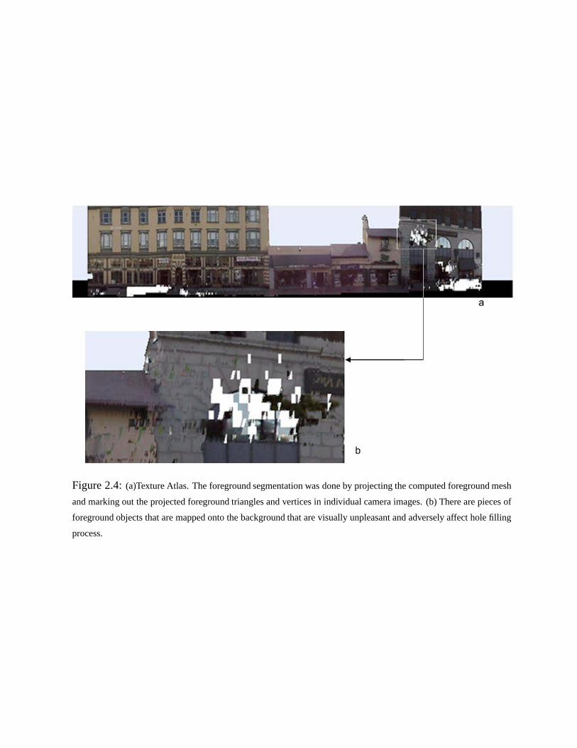
Figure 2.4: (a)Texture Atlas. The foreground segmentation was done by projecting the computed foreground mesh

and marking out the projected foreground triangles and vertices in individual camera images. (b) There are pieces of

foreground objects that are mapped onto the background that are visually unpleasant and adversely affect hole filling

process.

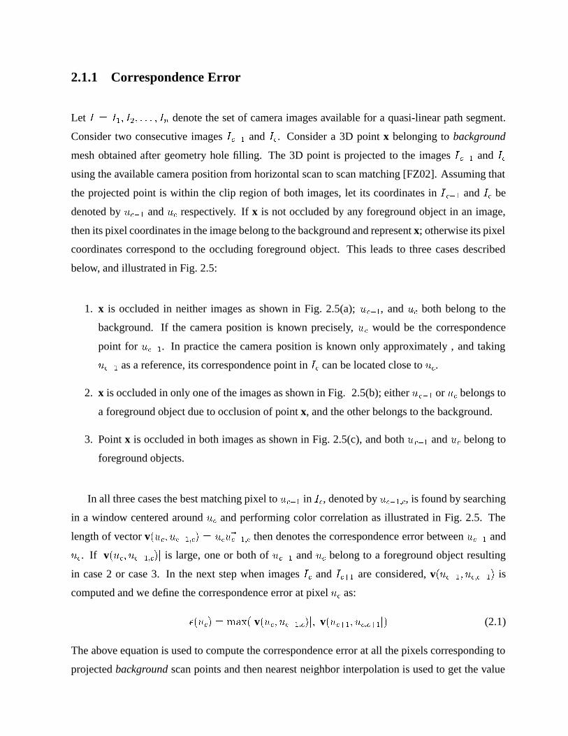
2.1.1 Correspondence Error

Let � � ��� ��� � � � � �� denote the set of camera images available for a quasi-linear path segment.

Consider two consecutive images ���� and ��. Consider a 3D point x belonging to background

mesh obtained after geometry hole filling. The 3D point is projected to the images ���� and ��

using the available camera position from horizontal scan to scan matching [FZ02]. Assuming that

the projected point is within the clip region of both images, let its coordinates in � ��� and �� be

denoted by ���� and �� respectively. If x is not occluded by any foreground object in an image,

then its pixel coordinates in the image belong to the background and represent x; otherwise its pixel

coordinates correspond to the occluding foreground object. This leads to three cases described

below, and illustrated in Fig. 2.5:

1. x is occluded in neither images as shown in Fig. 2.5(a); ����, and �� both belong to the

background. If the camera position is known precisely, �� would be the correspondence

point for ����. In practice the camera position is known only approximately , and taking

���� as a reference, its correspondence point in �� can be located close to ��.

2. x is occluded in only one of the images as shown in Fig. 2.5(b); either ���� or �� belongs to

a foreground object due to occlusion of point x, and the other belongs to the background.

3. Point x is occluded in both images as shown in Fig. 2.5(c), and both ���� and �� belong to

foreground objects.

In all three cases the best matching pixel to ���� in ��, denoted by ������, is found by searching

in a window centered around �� and performing color correlation as illustrated in Fig. 2.5. The

length of vector v���� ������� � ��������� then denotes the correspondence error between ���� and

��. If �v���� �������� is large, one or both of ���� and �� belong to a foreground object resulting

in case 2 or case 3. In the next step when images �� and ���� are considered, v������ ������� is

computed and we define the correspondence error at pixel �� as:

����� � �����v���� ��������� �v������ �������� (2.1)

The above equation is used to compute the correspondence error at all the pixels corresponding to

projected background scan points and then nearest neighbor interpolation is used to get the value

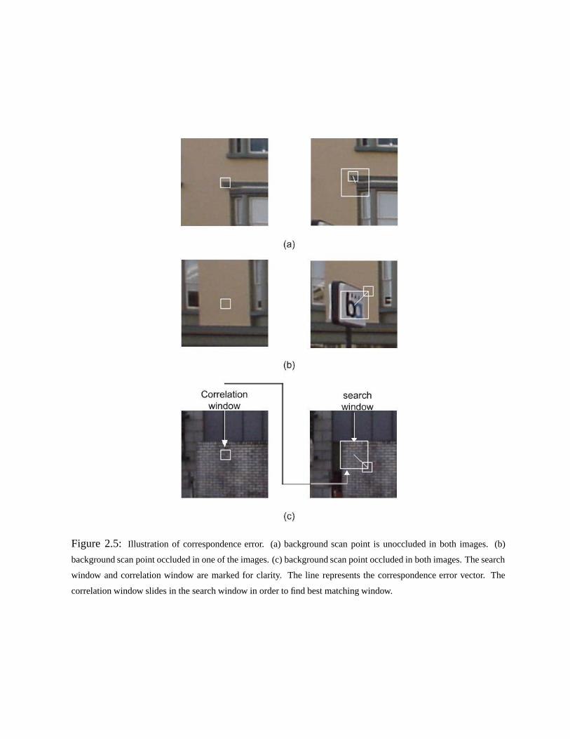
Figure 2.5: Illustration of correspondence error. (a) background scan point is unoccluded in both images. (b)

background scan point occluded in one of the images. (c) background scan point occluded in both images. The search

window and correlation window are marked for clarity. The line represents the correspondence error vector. The

correlation window slides in the search window in order to find best matching window.

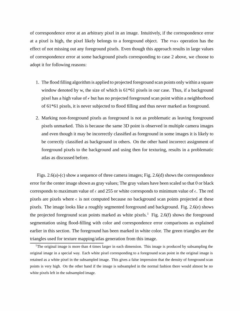
of correspondence error at an arbitrary pixel in an image. Intuitively, if the correspondence error

at a pixel is high, the pixel likely belongs to a foreground object. The ��� operation has the

effect of not missing out any foreground pixels. Even though this approach results in large values

of correspondence error at some background pixels corresponding to case 2 above, we choose to

adopt it for following reasons:

1. The flood filling algorithm is applied to projected foreground scan points only within a square

window denoted by w, the size of which is 61*61 pixels in our case. Thus, if a background

pixel has a high value of � but has no projected foreground scan point within a neighborhood

of 61*61 pixels, it is never subjected to flood filling and thus never marked as foreground.

2. Marking non-foreground pixels as foreground is not as problematic as leaving foreground

pixels unmarked. This is because the same 3D point is observed in multiple camera images

and even though it may be incorrectly classified as foreground in some images it is likely to

be correctly classified as background in others. On the other hand incorrect assignment of

foreground pixels to the background and using then for texturing, results in a problematic

atlas as discussed before.

Figs. 2.6(a)-(c) show a sequence of three camera images; Fig. 2.6(d) shows the correspondence

error for the center image shown as gray values; The gray values have been scaled so that 0 or black

corresponds to maximum value of � and 255 or white corresponds to minimum value of �. The red

pixels are pixels where � is not computed because no background scan points projected at these

pixels. The image looks like a roughly segmented foreground and background. Fig. 2.6(e) shows

the projected foreground scan points marked as white pixels.1 Fig. 2.6(f) shows the foreground

segmentation using flood-filling with color and correspondence error comparisons as explained

earlier in this section. The foreground has been marked in white color. The green triangles are the

triangles used for texture mapping/atlas generation from this image.1The original image is more than 4 times larger in each dimension. This image is produced by subsampling the

original image in a special way. Each white pixel corresponding to a foreground scan point in the original image is

retained as a white pixel in the subsampled image. This gives a false impression that the density of foreground scan

points is very high. On the other hand if the image is subsampled in the normal fashion there would almost be no

white pixels left in the subsampled image.

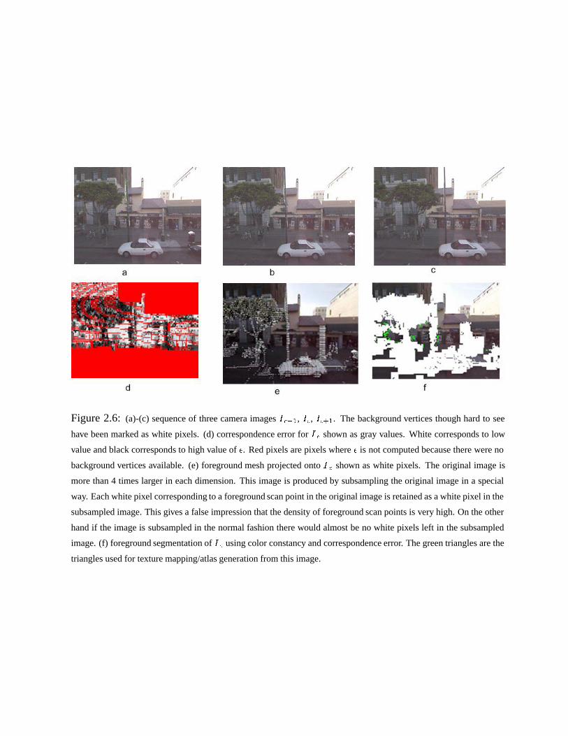
Figure 2.6: (a)-(c) sequence of three camera images ����, ��, ����. The background vertices though hard to see

have been marked as white pixels. (d) correspondence error for � � shown as gray values. White corresponds to low

value and black corresponds to high value of �. Red pixels are pixels where � is not computed because there were no

background vertices available. (e) foreground mesh projected onto � � shown as white pixels. The original image is

more than 4 times larger in each dimension. This image is produced by subsampling the original image in a special

way. Each white pixel corresponding to a foreground scan point in the original image is retained as a white pixel in the

subsampled image. This gives a false impression that the density of foreground scan points is very high. On the other

hand if the image is subsampled in the normal fashion there would almost be no white pixels left in the subsampled

image. (f) foreground segmentation of � � using color constancy and correspondence error. The green triangles are the

triangles used for texture mapping/atlas generation from this image.

As can be seen, there are some background pixels that have been incorrectly assigned to the

foreground. This is due to following reasons:

1. The projected foreground scan points sometimes correspond to background rather than fore-

ground due to errors. The algorithm described here assumes all pixels corresponding to

projected foreground scan points belong to the foreground. If only color comparison is used

for foreground segmentation then in such cases one will end up marking the background

instead of the foreground — the opposite of what is desired.

2. Since in our present application, assigning background pixels to the foreground (Type 1 er-

ror) is not as problematic as assigning foreground pixels to the background (Type 2 error), we

tune our parameters accordingly so that Type 1 errors rarely occur. This however increases

Type 2 errors.

The next section describes how after segmenting the foreground, multiple images are combined

into a single texture atlas that is finally used for texturing the background mesh.

2.2 Texture Atlas Generation

Since most parts of a camera image correspond to either foreground objects or facade areas visible

in other images at a more direct view, we can reduce the amount of texture imagery by extracting

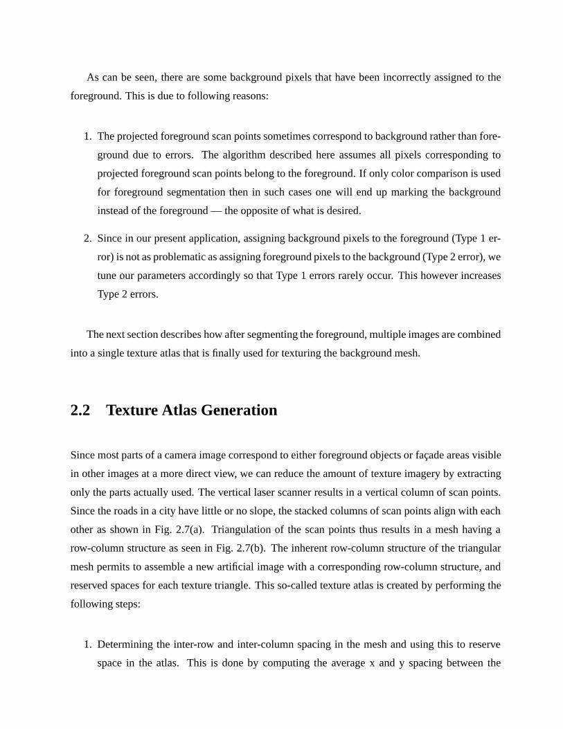
only the parts actually used. The vertical laser scanner results in a vertical column of scan points.

Since the roads in a city have little or no slope, the stacked columns of scan points align with each

other as shown in Fig. 2.7(a). Triangulation of the scan points thus results in a mesh having a

row-column structure as seen in Fig. 2.7(b). The inherent row-column structure of the triangular

mesh permits to assemble a new artificial image with a corresponding row-column structure, and

reserved spaces for each texture triangle. This so-called texture atlas is created by performing the

following steps:

1. Determining the inter-row and inter-column spacing in the mesh and using this to reserve

space in the atlas. This is done by computing the average x and y spacing between the

(a) (b)

Figure 2.7: (a) columns of background scan points (b) background mesh after triangulation of scan points. The scan

points are seen to form a rectangular grid and the triangles fit into the grid forming a row-column structure.

columns and rows of scan points respectively.

2. Warping each texture triangle by applying a linear transformation to the three vertices to fit

to the corresponding reserved space in the atlas and copying it into the atlas.

3. Setting texture coordinates of the mesh triangles to the location in the atlas.

Thus, rather than using numerous original images, we use atlas to represent the texture. Since in

this manner the mesh topology of the triangles is preserved and adjacent triangles align automati-

cally due to the warping process, the resulting texture atlas resembles a mosaic image. While the

atlas is in fact not precisely proportionate due to slightly non-uniform spacing between vertical

scans, these distortions are small and negligible in the context of texture mapping, since they are

inverted by the graphics card hardware during the rendering process.

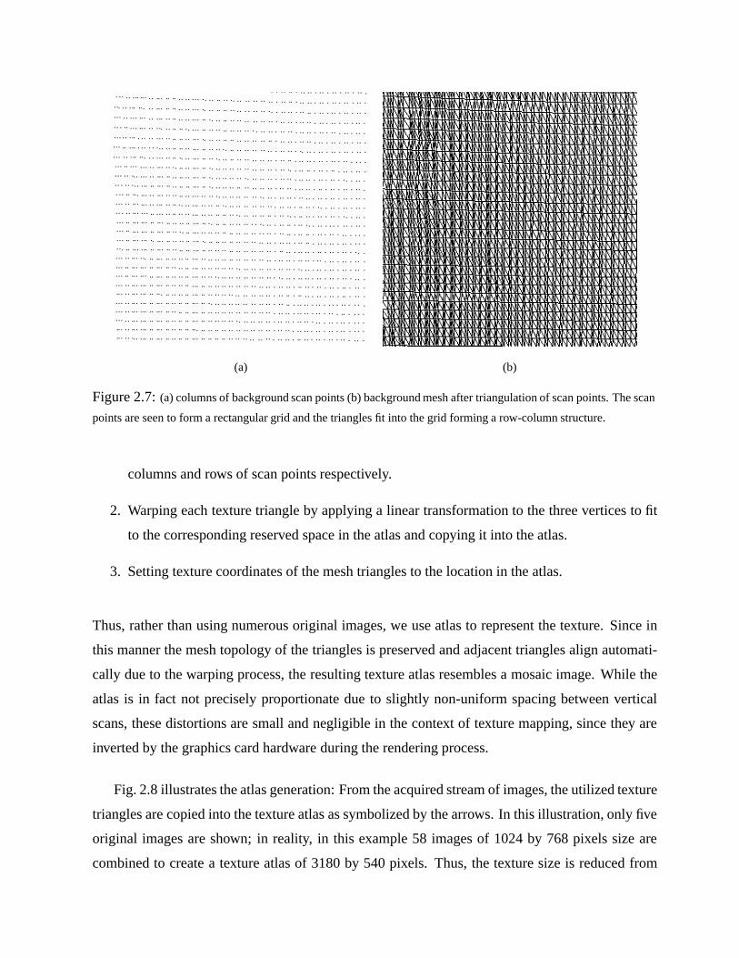
Fig. 2.8 illustrates the atlas generation: From the acquired stream of images, the utilized texture

triangles are copied into the texture atlas as symbolized by the arrows. In this illustration, only five

original images are shown; in reality, in this example 58 images of 1024 by 768 pixels size are

combined to create a texture atlas of 3180 by 540 pixels. Thus, the texture size is reduced from

45.6 million pixels to 1.7 million pixels, while the resolution remains the same.

If occluding foreground objects and building facade are too close, some facade triangles might

not be visible in any of the captured imagery, and hence cannot be texture mapped at all as seen in

Fig. 2.8(b). This leaves visually unpleasant holes in the texture atlas, and hence in final rendering

of the 3D models. In the next chapter we propose ways of synthesizing plausible artificial texture

for these holes that results in a filled in atlas as shown in Fig. 2.8(c).

Figure 2.8: (a) Images obtained after foreground segmentation are combined to create a texture atlas. In this

illustration only five images are shown, whereas in this particular example 58 images were combined to create the

texture atlas. The green triangles in an image represent the parts of the image that are actually inserted in the texture

atlas. (b) Atlas with texture holes due to occlusion from foreground objects. (c) Artificial texture is synthesized in the

texture holes to result in a filled in atlas that is finally used for texturing the background mesh.

Chapter 3

Hole Filling of the Atlases

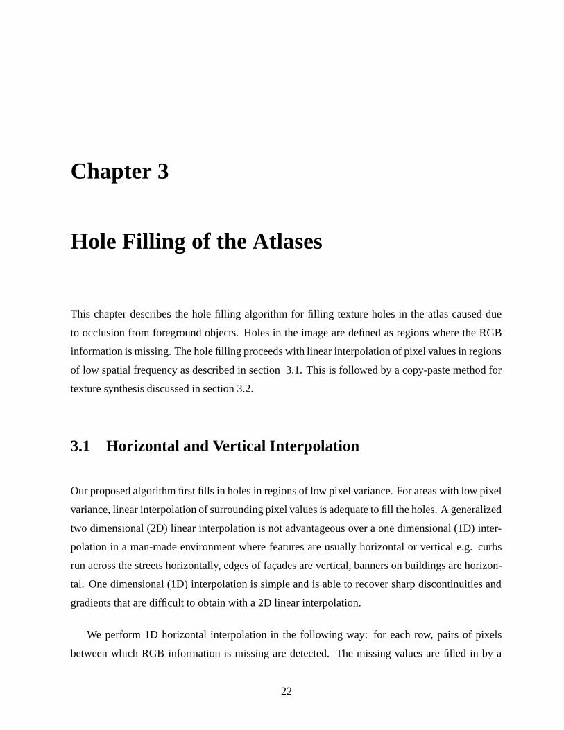
This chapter describes the hole filling algorithm for filling texture holes in the atlas caused due

to occlusion from foreground objects. Holes in the image are defined as regions where the RGB

information is missing. The hole filling proceeds with linear interpolation of pixel values in regions

of low spatial frequency as described in section 3.1. This is followed by a copy-paste method for

texture synthesis discussed in section 3.2.

3.1 Horizontal and Vertical Interpolation

Our proposed algorithm first fills in holes in regions of low pixel variance. For areas with low pixel

variance, linear interpolation of surrounding pixel values is adequate to fill the holes. A generalized

two dimensional (2D) linear interpolation is not advantageous over a one dimensional (1D) inter-

polation in a man-made environment where features are usually horizontal or vertical e.g. curbs

run across the streets horizontally, edges of facades are vertical, banners on buildings are horizon-

tal. One dimensional (1D) interpolation is simple and is able to recover sharp discontinuities and

gradients that are difficult to obtain with a 2D linear interpolation.

We perform 1D horizontal interpolation in the following way: for each row, pairs of pixels

between which RGB information is missing are detected. The missing values are filled in by a

22

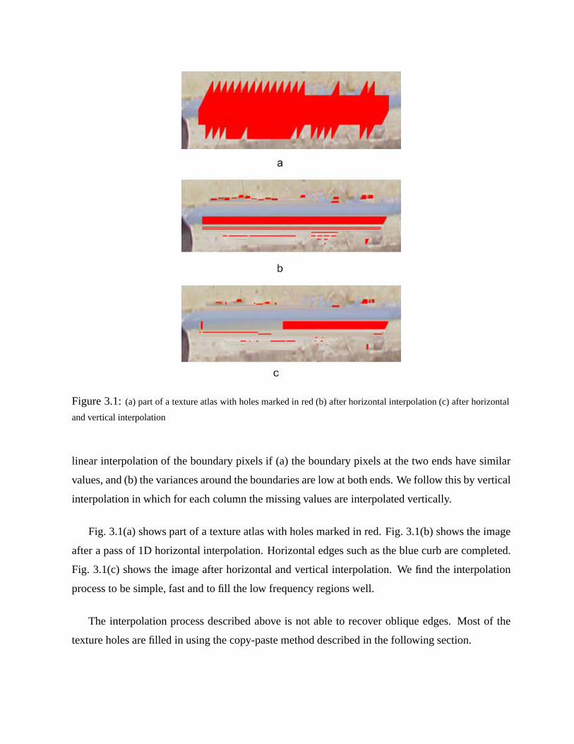
Figure 3.1: (a) part of a texture atlas with holes marked in red (b) after horizontal interpolation (c) after horizontal

and vertical interpolation

linear interpolation of the boundary pixels if (a) the boundary pixels at the two ends have similar

values, and (b) the variances around the boundaries are low at both ends. We follow this by vertical

interpolation in which for each column the missing values are interpolated vertically.

Fig. 3.1(a) shows part of a texture atlas with holes marked in red. Fig. 3.1(b) shows the image

after a pass of 1D horizontal interpolation. Horizontal edges such as the blue curb are completed.

Fig. 3.1(c) shows the image after horizontal and vertical interpolation. We find the interpolation

process to be simple, fast and to fill the low frequency regions well.

The interpolation process described above is not able to recover oblique edges. Most of the

texture holes are filled in using the copy-paste method described in the following section.

3.2 The Copy-Paste Method

After horizontal and vertical interpolation, the rest of the holes are filled by copying and pasting

blocks from other parts of the image. This is essentially the idea of texture synthesis in [EF01] in

which that authors create a large image with texture similar to a given template. In our copy-paste

method the image is scanned pixel by pixel in raster scan order and pixels at the boundary of holes

are stored in an array to be processed. A square window denoted by � of size 129*129 pixels is

taken centered at a hole pixel � and the image is searched for a window bestmatch��� which (a)

has the same size as � (b) lies in a search region �� which typically is a large window having same

center as � (c) does not contain more than 10% hole pixels and (d) matches best with �. If the

difference between � and bestmatch��� is below a threshold the bestmatch is classified as a good

match to � and hole pixels of � are replaced with corresponding pixels in bestmatch���. The

method is illustrated in Fig. 3.2. Fig. 4.2(a) shows a larger portion of the image and Fig. 4.2(b)

shows the result obtained by copying and pasting blocks from remainder of the image.

Following salient features of this method emerge:

� The method works well on holes in any kind of repetitive patterns, textures and smooth

regions.

� The method is able to detect and complete straight edges satisfactorily. Note this for example

in Fig. 4.5.

� The method does not suffer from the limitation of local inpainting.

� The method is capable of filling holes in an iterative fashion that are larger than the matching

window itself.

� There is an inherent assumption that there exists some region in the image which can be

copied and pasted over a hole — this actually turns out to be true in many natural images

such as building facades which are repetitive. Nevertheless there should be some strategy

of dealing with cases when there is no good match that can be copied and pasted. We use a

simple interpolation scheme that amounts to averaging the known neighbors and discussed

later in this section.

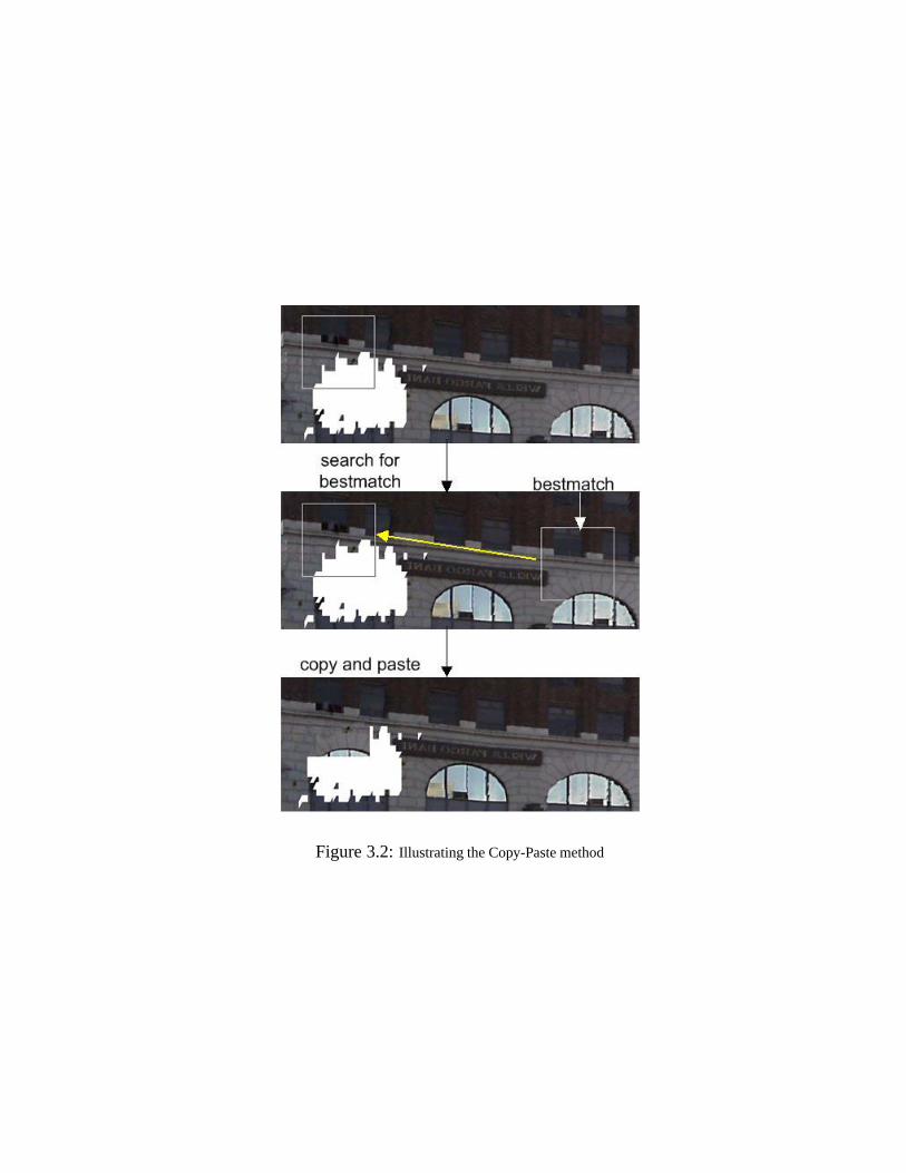
Figure 3.2: Illustrating the Copy-Paste method

G(x,y)� subsample� G(x,y)� subsample� G(x,y)� Subsample�I�o�

I�1�I�2�

I�n�

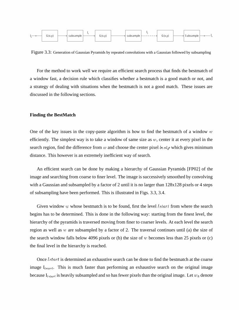
Figure 3.3: Generation of Gaussian Pyramids by repeated convolutions with a Gaussian followed by subsampling

For the method to work well we require an efficient search process that finds the bestmatch of

a window fast, a decision rule which classifies whether a bestmatch is a good match or not, and

a strategy of dealing with situations when the bestmatch is not a good match. These issues are

discussed in the following sections.

Finding the BestMatch

One of the key issues in the copy-paste algorithm is how to find the bestmatch of a window �

efficiently. The simplest way is to take a window of same size as �, center it at every pixel in the

search region, find the difference from � and choose the center pixel ��� which gives minimum

distance. This however is an extremely inefficient way of search.

An efficient search can be done by making a hierarchy of Gaussian Pyramids [FP02] of the

image and searching from coarse to finer level. The image is successively smoothed by convolving

with a Gaussian and subsampled by a factor of 2 until it is no larger than 128x128 pixels or 4 steps

of subsampling have been performed. This is illustrated in Figs. 3.3, 3.4.

Given window � whose bestmatch is to be found, first the level ����� from where the search

begins has to be determined. This is done in the following way: starting from the finest level, the

hierarchy of the pyramids is traversed moving from finer to coarser levels. At each level the search

region as well as � are subsampled by a factor of 2. The traversal continues until (a) the size of

the search window falls below 4096 pixels or (b) the size of � becomes less than 25 pixels or (c)

the final level in the hierarchy is reached.

Once ����� is determined an exhaustive search can be done to find the bestmatch at the coarse

image I������. This is much faster than performing an exhaustive search on the original image

because I������ is heavily subsampled and so has fewer pixels than the original image. Let �� denote

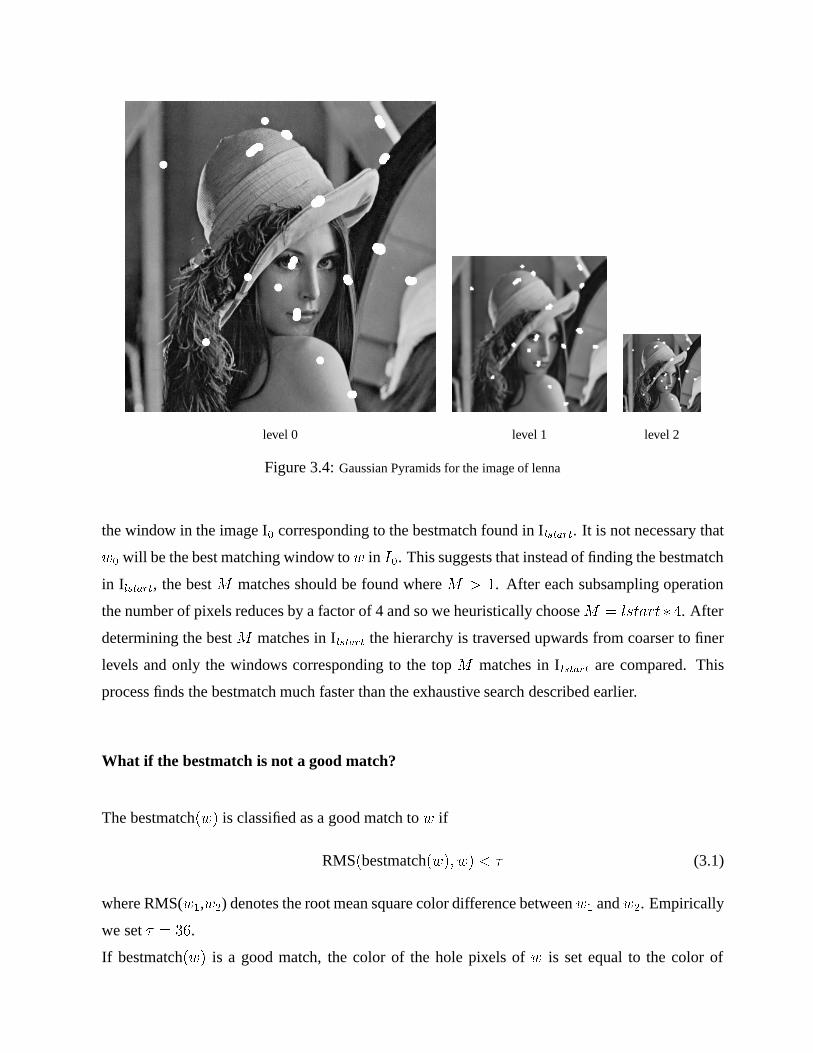
level 0 level 1 level 2

Figure 3.4: Gaussian Pyramids for the image of lenna

the window in the image I� corresponding to the bestmatch found in I������. It is not necessary that

�� will be the best matching window to � in ��. This suggests that instead of finding the bestmatch

in I������, the best � matches should be found where � � �. After each subsampling operation

the number of pixels reduces by a factor of 4 and so we heuristically choose � � ����� � �. After

determining the best � matches in I������ the hierarchy is traversed upwards from coarser to finer

levels and only the windows corresponding to the top � matches in I ������ are compared. This

process finds the bestmatch much faster than the exhaustive search described earlier.

What if the bestmatch is not a good match?

The bestmatch��� is classified as a good match to � if

RMS�bestmatch���� �� � � (3.1)

where RMS(��,��) denotes the root mean square color difference between �� and ��. Empirically

we set � � .

If bestmatch��� is a good match, the color of the hole pixels of � is set equal to the color of

corresponding pixels in bestmatch���. However if bestmatch��� is not a good match the window

size is made adaptive by reducing the size of � by 2 in both x, y directions and a search is performed

for the bestmatch of the new window. This process is continued until (a) a good match is found, or

(b) size of � becomes too small. Specifically for our texture atlases we start with window of size

129x129 pixels and keep finding the bestmatch until the size of window reduces to 9x9 pixels. For

other images we start with window of size 17x17 and continue until size of window reduces to 5x5

pixels. Most of the time the algorithm is able to find a bestmatch that is a goodmatch using this

adaptive scheme. However there are rare cases when no good match is found. In this case a simple

interpolation scheme described below is used.

Consider a hole pixel � � ��� ��. and a 3x3 window � centered at �. A simple interpolation

method would be to average the color of the non-hole pixels in � and assign this value to pixel �.

However if the colors of non-hole pixels in � differ substantially then rather than averaging, the

color of � can be set equal to the color of a randomly chosen non-hole pixel in �.

The next chapter discusses results of hole filling using the algorithm described in this chapter.

Chapter 4

Results and Remarks

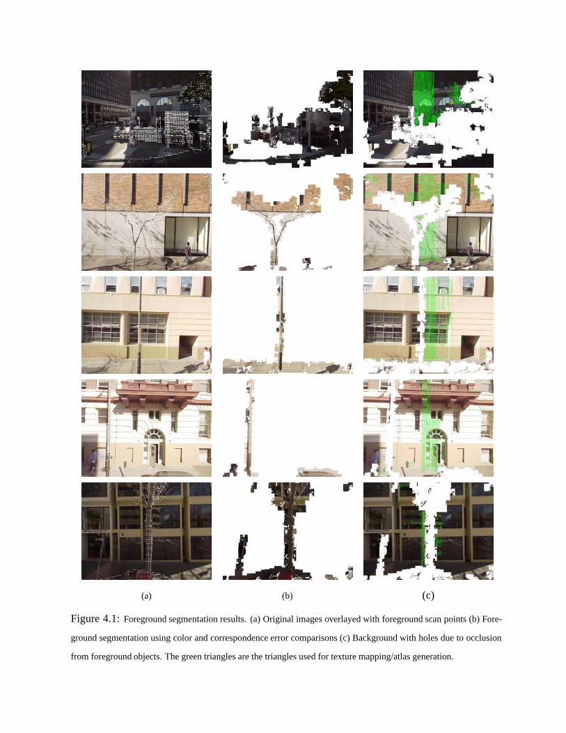
In this chapter we present some results on the foreground segmentation of images and hole filling

of images. Fig. 4.1 shows five examples of foreground segmentation of images. Column (a) of

the figure shows the original image overlayed with foreground scan points. Column (b) shows

the segmented foreground using flood filling and color and correspondence error comparisons as

described in section 2.1 and column (c) shows the background. As can be seen, there are some

background pixels that have been incorrectly assigned to the foreground. The reasons for this were

mentioned at the end of section 2.1.

Figs. 4.2-4.7 show hole filling results on some images. In these figures, the image with holes

marked in either red or white is shown as (a), the hole filled result using the method described in

chapter 3 is shown as (b) and for purposes of comparison the result using inpainting as described

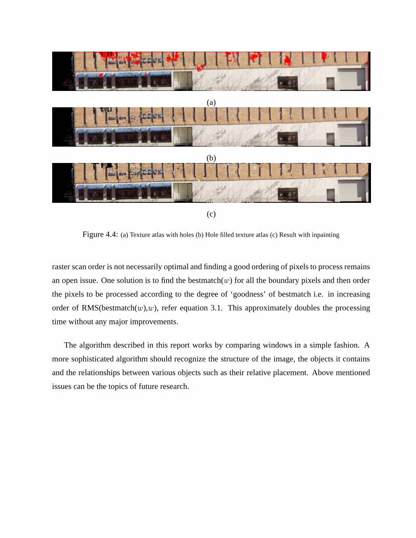
in [Ber01] is shown as (c). Figs. 4.2, 4.3, 4.4 show results of hole filling on texture atlases. Figs. 4.2

and 4.3 show portions of two texture atlases whereas Fig. 4.4 shows a complete texture atlas. As

seen in the hole filled images, the synthesized texture significantly improves the completeness

and visual appearance of the models. Fig. 4.2(a) shows an image with holes marked in white.

Fig. 4.2(b) shows the result obtained using the hole filling algorithm described in chapter 3. For

comparison, Fig. 4.2(c) shows the result obtained using the image inpainting method described in

[Ber01]. The copy-paste method is able to fill the hole in a better manner compared to inpainting,

by copying the arch from other parts of the image. The inpainting method utilizes only the pixel

information available in a thin band around the hole and therefore gives a result which looks like

29

(a) (b) (c)

Figure 4.1: Foreground segmentation results. (a) Original images overlayed with foreground scan points (b) Fore-

ground segmentation using color and correspondence error comparisons (c) Background with holes due to occlusion

from foreground objects. The green triangles are the triangles used for texture mapping/atlas generation.

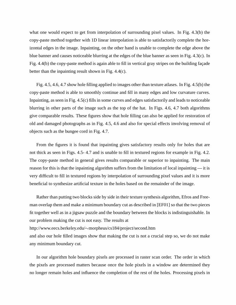
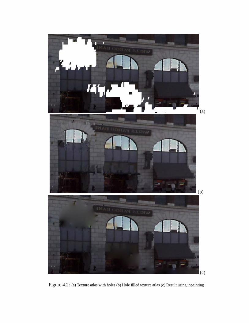
what one would expect to get from interpolation of surrounding pixel values. In Fig. 4.3(b) the

copy-paste method together with 1D linear interpolation is able to satisfactorily complete the hor-

izontal edges in the image. Inpainting, on the other hand is unable to complete the edge above the

blue banner and causes noticeable blurring at the edges of the blue banner as seen in Fig. 4.3(c). In

Fig. 4.4(b) the copy-paste method is again able to fill in vertical gray stripes on the building facade

better than the inpainting result shown in Fig. 4.4(c).

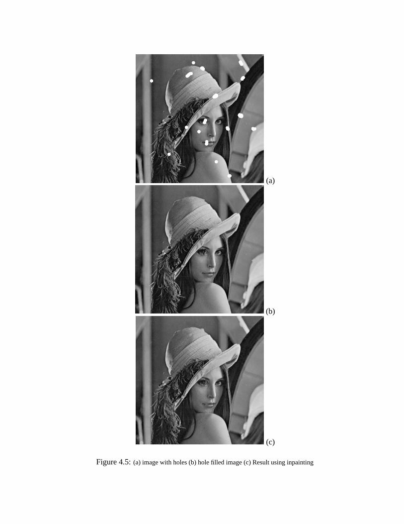
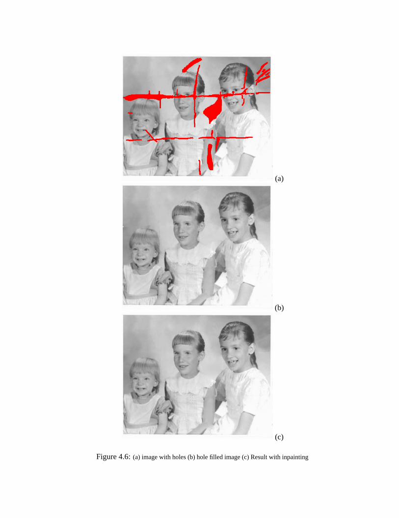
Fig. 4.5, 4.6, 4.7 show hole filling applied to images other than texture atlases. In Fig. 4.5(b) the

copy-paste method is able to smoothly continue and fill in many edges and low curvature curves.

Inpainting, as seen in Fig. 4.5(c) fills in some curves and edges satisfactorily and leads to noticeable

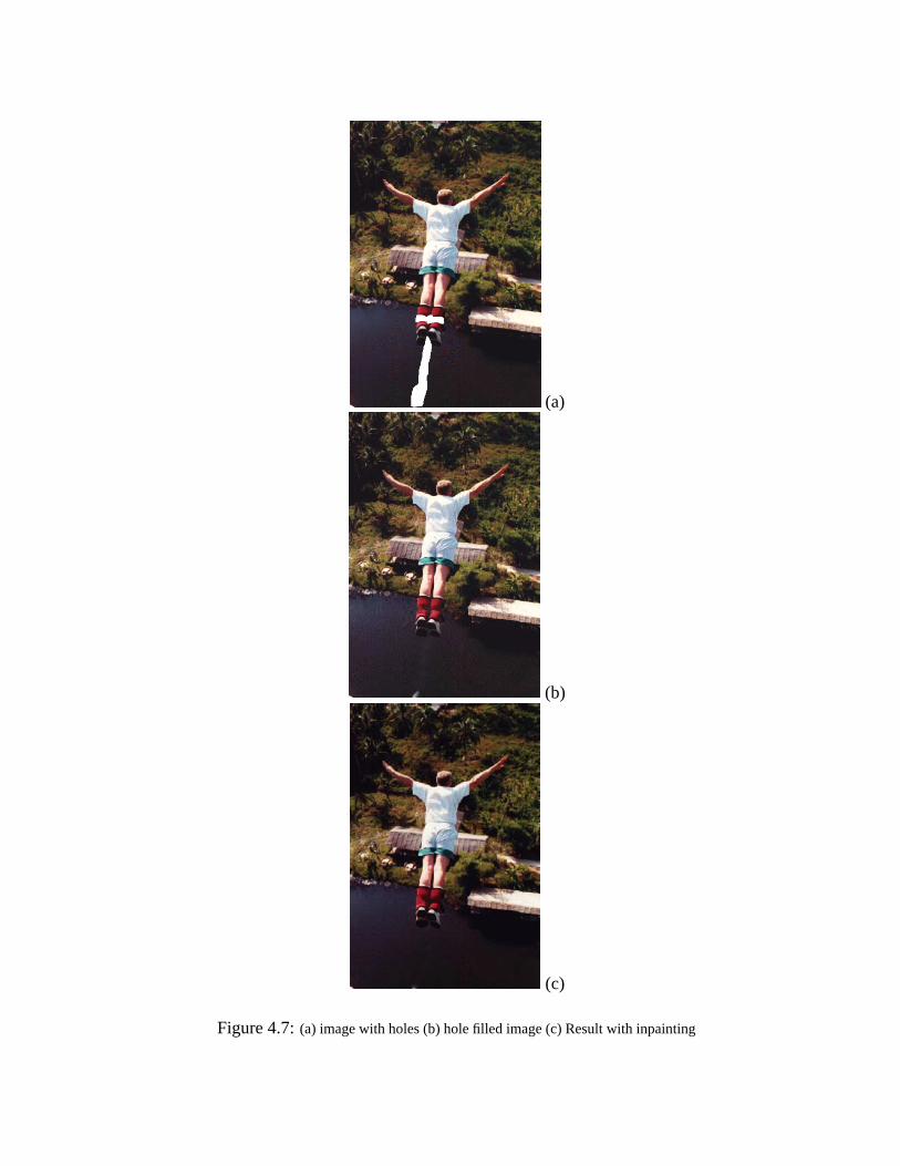
blurring in other parts of the image such as the top of the hat. In Figs. 4.6, 4.7 both algorithms

give comparable results. These figures show that hole filling can also be applied for restoration of

old and damaged photographs as in Fig. 4.5, 4.6 and also for special effects involving removal of

objects such as the bungee cord in Fig. 4.7.

From the figures it is found that inpainting gives satisfactory results only for holes that are

not thick as seen in Figs. 4.5- 4.7 and is unable to fill in textured regions for example in Fig. 4.2.

The copy-paste method in general gives results comparable or superior to inpainting. The main

reason for this is that the inpainting algorithm suffers from the limitation of local inpainting — it is

very difficult to fill in textured regions by interpolation of surrounding pixel values and it is more

beneficial to synthesize artificial texture in the holes based on the remainder of the image.

Rather than putting two blocks side by side in their texture synthesis algorithm, Efros and Free-

man overlap them and make a minimum boundary cut as described in [EF01] so that the two pieces

fit together well as in a jigsaw puzzle and the boundary between the blocks is indistinguishable. In

our problem making the cut is not easy. The results at

http://www.eecs.berkeley.edu/�morpheus/cs184/project/second.htm

and also our hole filled images show that making the cut is not a crucial step so, we do not make

any minimum boundary cut.

In our algorithm hole boundary pixels are processed in raster scan order. The order in which

the pixels are processed matters because once the hole pixels in a window are determined they

no longer remain holes and influence the completion of the rest of the holes. Processing pixels in

(a)

(b)

(c)

Figure 4.2: (a) Texture atlas with holes (b) Hole filled texture atlas (c) Result using inpainting

(a)

(b)

(c)

Figure 4.3: (a) Texture atlas with holes (b) Hole filled texture atlas (c) Result with inpainting

(a)

(b)

(c)

Figure 4.4: (a) Texture atlas with holes (b) Hole filled texture atlas (c) Result with inpainting

raster scan order is not necessarily optimal and finding a good ordering of pixels to process remains

an open issue. One solution is to find the bestmatch(�) for all the boundary pixels and then order

the pixels to be processed according to the degree of ‘goodness’ of bestmatch i.e. in increasing

order of RMS(bestmatch(�),�), refer equation 3.1. This approximately doubles the processing

time without any major improvements.

The algorithm described in this report works by comparing windows in a simple fashion. A

more sophisticated algorithm should recognize the structure of the image, the objects it contains

and the relationships between various objects such as their relative placement. Above mentioned

issues can be the topics of future research.

(a)

(b)

(c)

Figure 4.5: (a) image with holes (b) hole filled image (c) Result using inpainting

(a)

(b)

(c)

Figure 4.6: (a) image with holes (b) hole filled image (c) Result with inpainting

(a)

(b)

(c)

Figure 4.7: (a) image with holes (b) hole filled image (c) Result with inpainting

Bibliography

[AT00] M.E. Antone and S. Teller. Automatic recovery of relative camera rotations for ur-

ban scenes. In Proceedings IEEE International Conference on Computer Vision and

Pattern Recognition, pages 282–289, 2000.

[BBC�01] C. Ballester, M. Bertalmio, V. Caselles, G. Sapiro, and J. Verdera. Filling in by joint

interpolation of vector fields and gray levels. IEEE Trans. Image Processing, pages

1200–1211, August 2001.

[BCV�01] C. Ballester, V. Caselles, J. Verdera, M. Bertalmio, and G. Sapiro. A variational model

for filling-in gray level and color images. In Proc. 8th IEEE International Conference

on Computer Vision, volume 1, pages 10–16, 2001.

[Ber01] Marcelo Bertalmio. Processing of Flat and Non-Flat Image Information on Arbitrary

Manifolds using Partial Differential Equations. PhD thesis, University of Minnesota,

2001.

[BSCB00] Marcelo Bertalmio, Guillermo Sapiro, Vicent Caselles, and Coloma Ballester. Image

inpainting. In Kurt Akeley, editor, SIGGRAPH 2000, Computer Graphics Proceed-

ings, pages 417–424. ACM Press / ACM SIGGRAPH / Addison Wesley Longman,

2000.

[CS01] Tony Chan and Jianhong Shen. Mathematical models for local nontexture inpaintings.

SIAM Journal on Applied Mathematics, 62(3):1019–1043, 2001.

[EF01] Alexei A. Efros and William T. Freeman. Image quilting for texture synthesis and

transfer. In Eugene Fiume, editor, SIGGRAPH 2001, Computer Graphics Proceed-

ings, pages 341–346. ACM Press / ACM SIGGRAPH, 2001.

38

[FP02] D.A. Forsyth and J. Ponce. Computer Vision — A Modern Approach, chapter 7.

Prentice-Hall, 2002.

[Fru02] C. Fruh. Automated 3D Model Generation for Urban Environments. PhD thesis,

University of Freiburg, Germany, 2002.

[FvDFH95] J.D. Foley, A. van Dam, S.K. Fiener, and J.F. Hughes. Computer Graphics: Principles

and Practice, second edition in C, chapter 19. Addison-Wesley, Reading MA, 1995.

[FZ01a] C. Fruh and A. Zakhor. Fast 3D model generation in urban environments. In Inter-

national Conference on Multisensor Fusion and Integration for Intelligent Systems.

Baden-Baden, Germany, pages 165–170, August 2001.

[FZ01b] C. Fruh and A. Zakhor. 3D model generation for cities using aerial photographs and

ground level laser scans. In Computer Vision and Pattern Recognition Conference.

Kauai USA, volume 2, pages 31–38, December 2001.

[FZ02] C. Fruh and A. Zakhor. Data processing algorithms for generating textured 3D build-

ing facade meshes from laser scans and camera images. In Proceedings 3D Data

Processing, Visualization and Transmission. Padua, Italy, pages 834–847, June 2002.

[HBT01] D. Hahnel, W. Burgard, and S. Thrun. Learning compact 3D models of indoor and

outdoor environments with a mobile robot. In Fourth European Workshop on ad-

vanced mobile robots (EUROBOT’01), 2001.

[MM98] S. Masnou and J.M. Morel. Level-lines based disocclusion. In Fifth IEEE Interna-

tional Conference on Image Processing, pages 259–263, 1998.

[NMS93] M. Nitzberg, D. Mumford, and T. Shiota. Filtering, Segmentation and Depth.

Springer-Verlag, Berlin, 1993.

[SA00] I. Stamos and P.E. Allen. 3D model construction using range and image data. In

Proceedings IEEE International Conference on Computer Vision and Pattern Recog-

nition, pages 531–536, 2000.

[TBF00] S. Thrun, W. Burgard, and D. Fox. A real time algorithm for mobile robot mapping

with applications to multi-robot and 3D mappping. In Proceedings of IEEE Interna-

tional Conference on Robotics and Automation, pages 321–328, 2000.

[Tel98] S. Teller. Toward urban model acquisition from geo-located images. In Sixth Pacific

Conference on Computer Graphics and Applications, pages 45–52, 1998.

[ZS99] H. Zhao and R. Shibasaki. A system for reconstructing urban 3D objects using ground

based range and CCD images. In Proceedings of International Workshop on Urban

Multi-Media/3D Mapping, 1999.