video compression using vector quantization · video compression using vector quantization ......
TRANSCRIPT

by Mahesh Venkatraman, Heesung Kwon, and Nasser M. Nasrabadi
Video Compression using VectorQuantization
ARL-TR-1535 May 1998
Approved for public release; distribution unlimited.
The findings in this report are not to be construed as an official Department ofthe Army position unless so designated by other authorized documents.
Citation of manufacturer’s or trade names does not constitute an officialendorsement or approval of the use thereof.
Destroy this report when it is no longer needed. Do not return it to the originator.

Army Research LaboratoryAdelphi, MD 20783-1197
ARL-TR-1535 May 1998
Video Compression using VectorQuantizationMahesh Venkatraman, Heesung Kwon, and Nasser M. NasrabadiSensors and Electron Devices Directorate
Approved for public release; distribution unlimited.

Abstract
This report presents some results and findings of our work on very-low-bit-rate video compression systems using vector quantization (VQ). Wehave identified multiscale segmentation and variable-rate coding as twoimportant concepts whose effective use can lead to superior compressionperformance. Two VQ algorithms that attempt to use these two aspectsare presented: one based on residual vector quantization and the other onquadtree vector quantization. Residual vector quantization is a successiveapproximation quantizer technique and is ideal for variable-rate coding.Quadtree vector quantization is inherently a multiscale coding method.The report presents the general theoretical formulation of these algorithms,as well as quantitative performance of sample implementations.
ii

Contents
1 Introduction: Very-Low-Bit-Rate Video Coding for the DigitalBattlefield 1
2 Background 3
2.1 Quantization . . . . . . . . . . . . . . . . . . . . . . . . . . . . 3
2.2 Video Compression . . . . . . . . . . . . . . . . . . . . . . . . 4
2.3 Motion Compensation . . . . . . . . . . . . . . . . . . . . . . 4
3 Vector Quantization 6
3.1 Quantization Error of Vector Quantizers . . . . . . . . . . . . 7
3.2 Optimality Conditions for Vector Quantizers . . . . . . . . . 8
3.2.1 Nearest-Neighbor Condition . . . . . . . . . . . . . . 8
3.2.2 Centroid Condition . . . . . . . . . . . . . . . . . . . . 8
3.3 Design of Vector Quantizers . . . . . . . . . . . . . . . . . . . 9
3.3.1 Generalized Lloyd’s Algorithm . . . . . . . . . . . . . 9
3.3.2 Kohonen’s Self-Organizing Feature Map . . . . . . . 10
3.4 Entropy-Constrained Vector Quantizer . . . . . . . . . . . . . 10
3.5 Video Compression Using Vector Quantization . . . . . . . . 11
4 Residual Vector Quantization 13
4.1 Residual Quantization . . . . . . . . . . . . . . . . . . . . . . 13
4.2 Residual Vector Quantizer . . . . . . . . . . . . . . . . . . . . 14
4.3 Search Techniques for Residual Vector Quantizers . . . . . . 14
4.3.1 Exhaustive Search . . . . . . . . . . . . . . . . . . . . 15
4.3.2 Sequential Search . . . . . . . . . . . . . . . . . . . . . 15
4.3.3 M -Search . . . . . . . . . . . . . . . . . . . . . . . . . 15
4.4 Structure of Residual VQs . . . . . . . . . . . . . . . . . . . . 15
iii

4.5 Optimality Conditions for Residual Quantizers . . . . . . . . 16
4.5.1 Overall Optimality . . . . . . . . . . . . . . . . . . . . 16
4.5.2 Causal Stages Optimality . . . . . . . . . . . . . . . . 17
4.5.3 Simultaneous Causal and Overall Optimality . . . . . 18
4.6 Design of Residual Vector Quantizers . . . . . . . . . . . . . 19
4.7 Residual Vector Quantization with Variable Block Size . . . . 19
4.8 Pruned Variable-Block-Size Residual Vector Quantizer . . . . 19
4.8.1 Top-Down Pruning Using a Predefined Threshold . . 20
4.8.2 Optimal Pruning in the Rate-Distortion Sense . . . . 20
4.9 Transform-Domain Vector Quantization for Large Blocks . . 20
4.10 Video Compression Using Residual Vector Quantization . . 21
4.10.1 Theory of Residual Vector Quantization . . . . . . . . 21
4.10.2 Performance of an RVQ-Based Video Codec . . . . . 24
5 Quadtree-Based Vector Quantization 30
5.1 Quadtree Decomposition . . . . . . . . . . . . . . . . . . . . . 30
5.2 Optimal Quadtree in the Rate-Distortion Sense . . . . . . . . 31
5.3 Video Compression Using Quadtree-Based Vector Quantiza-tion . . . . . . . . . . . . . . . . . . . . . . . . . . . . . . . . . 32
6 Conclusions 33
References 34
Distribution 37
Report Documentation Page 41
iv

Figures
1 Original and compressed representations of a frame from aFLIR video sequence . . . . . . . . . . . . . . . . . . . . . . . 2
2 Scalar quantizer Q of a random variable Xn . . . . . . . . . . 4
3 Motion compensation for video coding . . . . . . . . . . . . 5
4 Entropy of a sequence after decorrelation in temporal dimen-sion . . . . . . . . . . . . . . . . . . . . . . . . . . . . . . . . . 5
5 Encoder/decoder model of a VQ . . . . . . . . . . . . . . . . 7
6 Entropy coding of VQ indices . . . . . . . . . . . . . . . . . . 10
7 VQ encoder for two-dimensional arrays . . . . . . . . . . . . 11
8 VQ decoder for two-dimensional arrays . . . . . . . . . . . . 12
9 Residual quantizer—cascade of two quantizers . . . . . . . . 14
10 Structure of a residual VQ . . . . . . . . . . . . . . . . . . . . 16
11 Tree structure of variable-block-size residual VQ . . . . . . . 19
12 Optimal pruning of residual VQ in rate-distortion sense . . . 21
13 Video encoder based on residual vector quantization . . . . 22
14 Video decoder based on residual vector quantization . . . . 23
15 Performance of video compression algorithms using vectorquantization . . . . . . . . . . . . . . . . . . . . . . . . . . . . 26
16 Results for bit rate of approximately 12 kb/s . . . . . . . . . 27
17 Results for bit rate of approximately 8.1 kb/s . . . . . . . . . 28
18 Results for bit rate of approximately 5.3 kb/s . . . . . . . . . 29
19 Vector quantization of quadtree leaf nodes . . . . . . . . . . 31
20 Encoding quadtree data structure . . . . . . . . . . . . . . . . 32
v

1. Introduction: Very-Low-Bit-Rate Video Coding for the DigitalBattlefield
Battlefield digitization—the process of representing all components of abattlefield in digital form—allows the battlefield and its components tobe visualized, simulated, and processed on computer systems, making theArmy more deadly and reducing the use of physical resources. For com-plete battlefield digitization, images of various modalities must be gath-ered by different imaging techniques. These images are then processed toprovide important information about the imaged areas.
An important class of visual data is the image sequence or video, andforward-looking infrared (FLIR) video is an important source of informa-tion. These data consist of a series of two-dimensional images capturedat a constant temporal rate. The main drawback to effective use of thisdata source is the huge amount of raw digital data (bits) required to repre-sent them. This volume of data makes real-time gathering and transmissionover tactical internets impractical.
To effectively combat this problem, data compression is used: that is, tech-niques to reduce the number of bits required to represent the data. Thelarge compression ratios needed to ”squeeze” video over low-bandwidthdigital channels require the use of ”lossy” image compression techniques.Lossy compression techniques use a very small number of bits to representthe data at the cost of degraded information. These techniques require atrade-off between video quality and bit-rate constraints.
For intelligent compression of FLIR video images, the bit assignment shouldbe made so that more bits are assigned to active areas, while fewer are as-signed to passive background areas. Vector quantization (a block quantiza-tion technique) has this type of adaptability, so that it is highly suitable forcompressing FLIR video.
In the work reported here, we systematically study the use of vector quan-tization for compressing video sequences. Results are shown for both FLIRvideo and regular gray-scale video. (A single representative frame of theoriginal FLIR video scene and its compressed representation are shown infig. 1.) We specifically study two adaptive vector quantization techniques:the residual vector quantizer (VQ) and the quadtree VQ. These two tech-niques permit the encoding of sources at different levels of precision de-pending on content.
1

Figure 1. Original (top) and compressed (bottom) representations of a frame from a FLIRvideo sequence.
The targeted bit rate is in the very low (5 to 16 kb/s) range; this rate allowsthe compressed video to be transmitted over SINCGARS (Single-ChannelGround to Air Radio System) channels, as well as permitting multiple videostreams to be multiplexed and transmitted over Fractional T1 lines. Suchmultiplex transmission would allow the video to be collected by sourcessuch as unmanned airborne vehicles (UAVs) and transmitted to processingcenters in real time.
2
2. Background
Images are represented in the digital domain by a matrix/array of intensityvalues, and video sequences are represented by a series of matrices. Thesematrices are often large, requiring large amounts of storage space and/ortransmission bandwidth. When resources are limited (storage spaces orbandwidth), it is essential to reduce the amount of data necessary for repre-senting the digital imagery. Data can be reduced (compressed) either withno loss in data (lossless compression) or with some degradation/distortionof the data (lossy compression). In lossless compression, redundancy in thedata is removed, resulting in a smaller representation, but the ratio of com-pression that can be achieved is small. On the other hand, lossy compres-sion techniques trade off the compression ratio against the tolerated dis-tortion. Most current image- and video-compression techniques are lossy,since human visual perception can tolerate a certain amount of distortion inthe presented visual data. Lossy compression can be achieved by quantiza-tion, a lossy compression technique in which data are represented at lowernumerical precision than in the original representation.
2.1 Quantization
A quantization Q of a random variable X ∈ R is a mapping from R to C, afinite subset ofR:
Q : R 7→ C, C ⊂ R. (1)
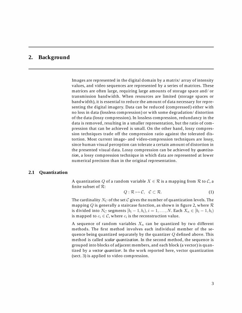
The cardinalityNC of the set C gives the number of quantization levels. Themapping Q is generally a staircase function, as shown in figure 2, whereRis divided into NC segments [bi − 1, bi), i = 1, . . . , N . Each Xn ∈ [bi − 1, bi)is mapped to ci ∈ C, where ci is the reconstruction value.
A sequence of random variables Xn can be quantized by two differentmethods. The first method involves each individual member of the se-quence being quantized separately by the quantizer Q defined above. Thismethod is called scalar quantization. In the second method, the sequence isgrouped into blocks of adjacent members, and each block (a vector) is quan-tized by a vector quantizer. In the work reported here, vector quantization(sect. 3) is applied to video compression.
3
bn–3 bn–2 bn–1
cn–2
cn–1
cn–1
cn–2
bn bn–1 bn–2
Xn
Q(Xn)
Figure 2. Scalar quantizer Q of a random variable Xn.
2.2 Video Compression
A video sequence is a three-dimensional signal of light intensity, with twospatial dimensions and a temporal dimension. A digital video sequence isa three-dimensional signal that is suitably sampled in all three dimensions;it is in the form of a three-dimensional matrix of intensity values. A typicalvideo sequence has a significant amount of correlation between neighborsin all three dimensions. The type of correlation in the temporal dimensionis significantly different from that in the spatial dimensions.
There are many different approaches to video compression, and some in-ternational compression standards have been established. Among the dif-ferent approaches is a class of algorithms that first attempt to remove cor-relations in the temporal domain and then deal with removing correlationsin the spatial dimensions. Among these is motion compensation (MC), apopular technique to remove the correlations in the temporal domain. Mo-tion compensation results in a residue sequence, which is then quantizedby two-dimensional quantization techniques similar to those used for com-pressing still images.
2.3 Motion Compensation
A video scene usually contains some motion of objects, occlusion/exposureof areas due to such motion, and some deformation. The rate of thesechanges is typically much smaller than the frame rate (i.e., the rate of sam-pling in the temporal dimension). Therefore, there is very little change be-tween two adjacent frames. A motion-compensation algorithm exploits thisconsistency to approximate the current frame by using pieces from theprevious frame. The result is a reasonable approximation of the currentframe based on the previous one, with some side information in the formof motion vectors. The difference between the approximation of the cur-rent frame and the actual frame is quantized by a set of scalar or vectorquantizers.
4
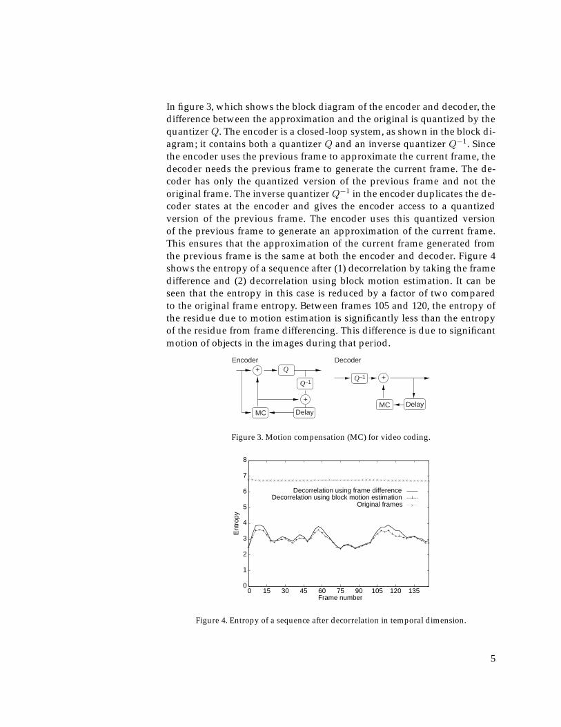
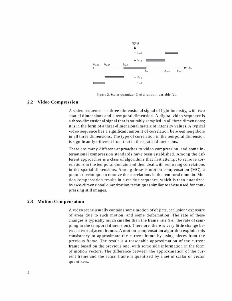
In figure 3, which shows the block diagram of the encoder and decoder, thedifference between the approximation and the original is quantized by thequantizer Q. The encoder is a closed-loop system, as shown in the block di-agram; it contains both a quantizer Q and an inverse quantizer Q−1. Sincethe encoder uses the previous frame to approximate the current frame, thedecoder needs the previous frame to generate the current frame. The de-coder has only the quantized version of the previous frame and not theoriginal frame. The inverse quantizerQ−1 in the encoder duplicates the de-coder states at the encoder and gives the encoder access to a quantizedversion of the previous frame. The encoder uses this quantized versionof the previous frame to generate an approximation of the current frame.This ensures that the approximation of the current frame generated fromthe previous frame is the same at both the encoder and decoder. Figure 4shows the entropy of a sequence after (1) decorrelation by taking the framedifference and (2) decorrelation using block motion estimation. It can beseen that the entropy in this case is reduced by a factor of two comparedto the original frame entropy. Between frames 105 and 120, the entropy ofthe residue due to motion estimation is significantly less than the entropyof the residue from frame differencing. This difference is due to significantmotion of objects in the images during that period.
+
MC
+
DelayDelay
Q
+
MC
Q–1Q–1
Encoder Decoder
Figure 3. Motion compensation (MC) for video coding.
0
1
2
3
4
5
6
7
8
0 15 30 45 60 75 90 105 120 135
Ent
ropy
Frame number
Decorrelation using frame differenceDecorrelation using block motion estimation
Original frames
Figure 4. Entropy of a sequence after decorrelation in temporal dimension.
5

3. Vector Quantization
A vector quantizerQ is a mapping from a point in k-dimensional Euclideanspace Rk into a finite subset C of Rk containing N reproduction points orvectors:
Q : Rk 7→ C.TheN reproduction vectors are called codevectors, and the set C is called thecodebook. C = (c1, c2, . . . , cn), and ci ∈ Rk for each i ∈ T = {1, 2, . . . , N}.The codebook C has N distinct members. The rate of the VQ, r = log2(N),measures the number of bits required to index a member of the codebook.
A VQ partitions the spaceRk into cellsRi:
Ri = {X ∈ Rk : Q(X) = ci}∀i ∈ T.
These cells represent the pre-image of the points ci under the mapping Q,i.e.,Ri = Q−1(ci). These cells have the following properties:
∪iRi = Rk,
Ri ∩Rj = {∅}∀i 6= j.
These properties imply that the cells are disjoint and that they cover theentire spaceRk.
The VQs dealt with here have the following additional properties:
• They are regular. The cells of a regular VQ, Ri, are convex, and ci ∈Ri.• They are polytopal. The cells of a polytopal VQ are polytopal. Poly-
topes are geometric regions bounded by hyperplane surfaces. A poly-topal region is the intersection of a finite number of subspaces.
• They are bounded. A VQ is bounded if it is defined on a boundeddomain B ⊂ Rk; i.e., every input vector X lies in B.
A VQ consists of two operators, an encoder and a decoder. The encoderγ associates every input vector X to i, which is some member of the in-dex set T . The decoder β associates the index i to ci, some member of thereproduction set C:
6

γ : Rk 7→ T,
β : T 7→ Rk,Q(X) = β(γ(X)).
The block diagram of the VQ is shown in figure 5. The encoding operationis completely determined by the partition of the input space. The encoderidentifies the cell to which a given input vector belongs. The decoding op-eration is determined by the codebook. Given the cell to which the inputvector belongs, the decoder determines the reproduction vector that bestrepresents the input vector. The decoder is very often in the form of a sim-ple lookup table. Given the index, the table returns the vector entry corre-sponding to the index.
Encoder DecoderiX Q(X)Inputvector
Channelsymbol
γ β Approximation ofinput vector
Figure 5. Encoder/decoder model of a VQ.
3.1 Quantization Error of Vector Quantizers
The performance of a VQ can be evaluated by the average distortion in-troduced by encoding a set of training input vectors. Ideally, the distortionshould be zero. The output of the decoder should be a close representationof the input vector. The expected value of the distortion measure representsthe performance of the quantizer:
D = E(d(X, Q(X))),
where d(X, Q(X)) represents the distortion introduced by the quantizer forthe input vector X.
One important distortion measure is the squared-error distortion measure(Euclidean distortion/L2 distortion). This distortion measure is especiallyrelevant to image coding problems, where the mean squared error is widelyused as a quantitative measure of the performance of coding:
d(X, Q(X)) = ||X−Q(X)||2,D = E(||X−Q(X)||2).
Other distortion measures include the weighed squared-error distortionmeasure, the Mahalanobis distortion measure, and the Itakura-Saito dis-tortion measure.
7
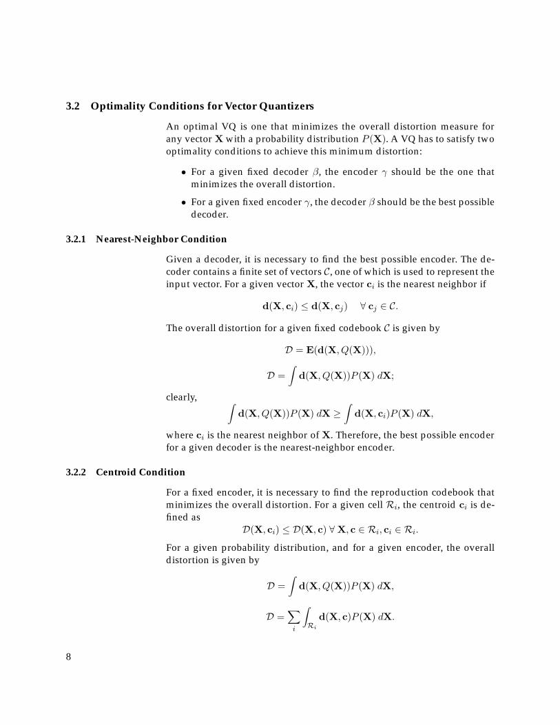
3.2 Optimality Conditions for Vector Quantizers
An optimal VQ is one that minimizes the overall distortion measure forany vector X with a probability distribution P (X). A VQ has to satisfy twooptimality conditions to achieve this minimum distortion:
• For a given fixed decoder β, the encoder γ should be the one thatminimizes the overall distortion.
• For a given fixed encoder γ, the decoder β should be the best possibledecoder.
3.2.1 Nearest-Neighbor Condition
Given a decoder, it is necessary to find the best possible encoder. The de-coder contains a finite set of vectors C, one of which is used to represent theinput vector. For a given vector X, the vector ci is the nearest neighbor if
d(X, ci) ≤ d(X, cj) ∀ cj ∈ C.
The overall distortion for a given fixed codebook C is given by
D = E(d(X, Q(X))),
D =∫
d(X, Q(X))P (X) dX;
clearly, ∫d(X, Q(X))P (X) dX ≥
∫d(X, ci)P (X) dX,
where ci is the nearest neighbor of X. Therefore, the best possible encoderfor a given decoder is the nearest-neighbor encoder.
3.2.2 Centroid Condition
For a fixed encoder, it is necessary to find the reproduction codebook thatminimizes the overall distortion. For a given cell Ri, the centroid ci is de-fined as
D(X, ci) ≤ D(X, c) ∀X, c ∈ Ri, ci ∈ Ri.For a given probability distribution, and for a given encoder, the overalldistortion is given by
D =∫
d(X, Q(X))P (X) dX,
D =∑i
∫Ri
d(X, c)P (X) dX.
8

Clearly,
∑i
∫Ri
d(X, c)P (X) dX ≥∑i
∫Ri
d(X, ci)P (X) dX.
Therefore, for a given encoder, the optimum decoder is the centroid of thenearest-neighbor partitions.
Consider the set A of all possible partitions of the input vectors, and a col-lection Co of all possible reproduction sets. The optimum VQ is the pair
({Ri}, C); {Ri} ∈ A and C ∈ Co,
such that Ri is the nearest neighbor partition of C that contains the cen-troids of the partitions in Ri. These two conditions are generalizations ofthe Lloyd-Max conditions for scalar quantizers.
3.3 Design of Vector Quantizers
Design of VQs is a very difficult problem. For a given probability dis-tribution P (X), it is necessary to find the encoder and decoder that si-multaneously satisfy both the nearest-neighbor condition and the centroidcondition. Unfortunately, no closed-form solutions exist for even simpledistributions.
A number of methods have been proposed for the design of VQs. All theseare iterative methods based on finding the best VQ for a training set.
3.3.1 Generalized Lloyd’s Algorithm
The generalized Lloyd’s algorithm (GLA) (also known as the LBG algo-rithm after Linde, Buzo, and Gray [1]) is an iterative algorithm. This algo-rithm, which is similar to the k-means clustering algorithm, consists of twobasic steps:
• For a given codebook Ct, find the best partition {Ri}t of the trainingset satisfying the nearest-neighbor neighborhood condition.
• For the new partition {Ri}t, find the best reproduction codebook Ct+1
satisfying the centroid condition.
These two steps are repeated until the required codebook is obtained. Thetraining algorithm begins with an initial codebook, which is refined by theLloyd’s iterations until an acceptable codebook is obtained. A codebook isconsidered acceptable if the error difference between the present and theprevious codebooks is less than a threshold.
9
3.3.2 Kohonen’s Self-Organizing Feature Map
Kohonen’s self-organizing feature maps (KSOFMs) can be used to designVQs with optimal codebooks [2,3]. In this method of codebook design, anenergy function for error is formulated and minimized iteratively. This de-sign procedure is sequential, unlike GLA, which uses the batch method oftraining.
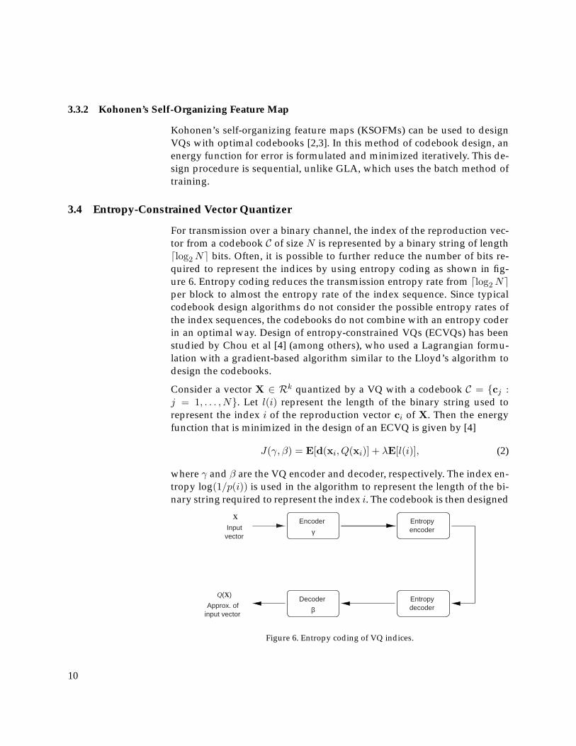
3.4 Entropy-Constrained Vector Quantizer
For transmission over a binary channel, the index of the reproduction vec-tor from a codebook C of size N is represented by a binary string of lengthdlog2Ne bits. Often, it is possible to further reduce the number of bits re-quired to represent the indices by using entropy coding as shown in fig-ure 6. Entropy coding reduces the transmission entropy rate from dlog2Neper block to almost the entropy rate of the index sequence. Since typicalcodebook design algorithms do not consider the possible entropy rates ofthe index sequences, the codebooks do not combine with an entropy coderin an optimal way. Design of entropy-constrained VQs (ECVQs) has beenstudied by Chou et al [4] (among others), who used a Lagrangian formu-lation with a gradient-based algorithm similar to the Lloyd’s algorithm todesign the codebooks.
Consider a vector X ∈ Rk quantized by a VQ with a codebook C = {cj :j = 1, . . . , N}. Let l(i) represent the length of the binary string used torepresent the index i of the reproduction vector ci of X. Then the energyfunction that is minimized in the design of an ECVQ is given by [4]
J(γ, β) = E[d(xi, Q(xi)] + λE[l(i)], (2)
where γ and β are the VQ encoder and decoder, respectively. The index en-tropy log(1/p(i)) is used in the algorithm to represent the length of the bi-nary string required to represent the index i. The codebook is then designed
Encoder
γ
Decoder
β
X
Inputvector
Q(X)
Approx. ofinput vector
Entropyencoder
Entropydecoder
Figure 6. Entropy coding of VQ indices.
10

in an iterative manner, similar to the Lloyd’s algorithm, through choosingan encoder and decoder that decrease the energy function in equation (2)at every iteration. Experimental results have shown that the ECVQ designalgorithm described above gives an encoder-decoder pair that has superiornumerical performance.
3.5 Video Compression Using Vector Quantization
The residual signal obtained after motion compensation can be compressedby vector quantization. The two-dimensional signal is divided into blocksof equal size, as shown in figure 7. The VQ encoder that is used to compressthe residual signal is a nearest-neighbor encoder. It has a reference lookuptable that contains the centroids of the VQ partitions. The encoder com-pares each block (in some predefined scanning order) with each memberof the lookup table to find the closest match in terms of the defined dis-tortion measure (usually the mean-squared error). The index of the closestmatching codevector in the lookup table is then transmitted/stored as thecompressed representation of the corresponding vector (block).
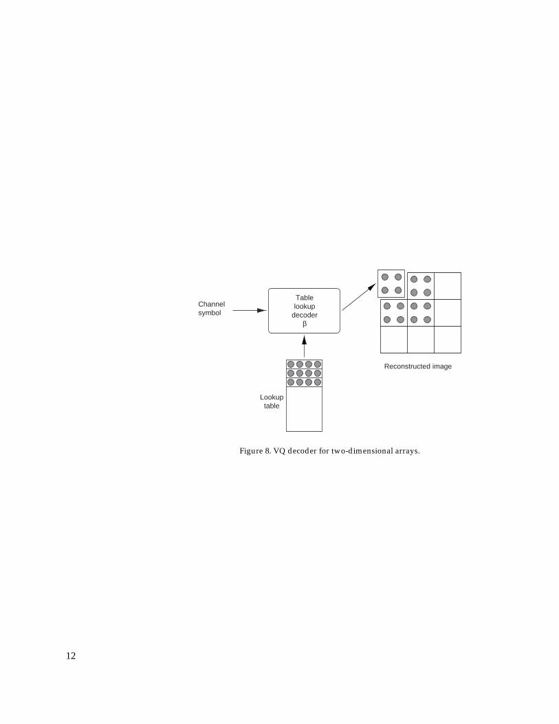
The decoder is a simple lookup table decoder, as shown in figure 8. Thedecoder uses the index symbol generated by the encoder as a reference toan entry in a lookup table in the decoder. The lookup table in the decoderis usually identical to the one in the encoder. This lookup table contains thepossible approximations for the blocks in the reconstructed image. Basedon the index, the approximate representation of the current block is deter-mined. To generate the reconstructed two-dimensional array, the decoderplaces this representation at the position corresponding to the scanning or-der. The reconstructed array is used along with the motion-compensationalgorithm to reproduce the compressed video sequence.
γ
Image divided into blocks
Nearest-neighborencoder
γ
Lookuptable
Channelsymbol
Figure 7. VQ encoder for two-dimensional arrays.
11
Channelsymbol
Reconstructed image
Tablelookup
decoderβ
Lookuptable
Figure 8. VQ decoder for two-dimensional arrays.
12
4. Residual Vector Quantization
Residual vector quantization (RVQ) is a structured vector quantizationscheme proposed mainly to overcome the search and storage complexitiesof regular VQs [5,6]. Residual VQs are also known as multistage VQs. Theyconsist of a number of cascaded VQs. Each stage has a VQ with a smallcodebook that quantizes the error signal from the previous stage. Residualquantizers are successive-refinement quantizers, where the information tobe transmitted/stored is first approximated coarsely and then refined inthe successive stages.
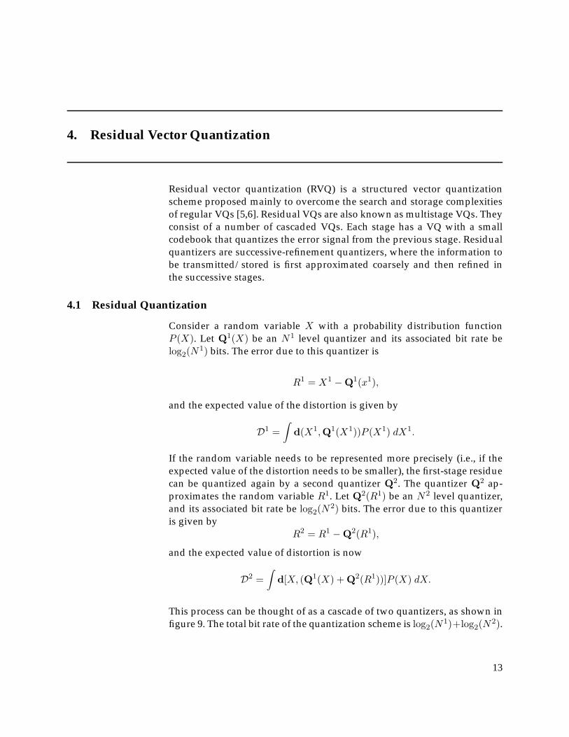
4.1 Residual Quantization
Consider a random variable X with a probability distribution functionP (X). Let Q1(X) be an N1 level quantizer and its associated bit rate belog2(N1) bits. The error due to this quantizer is
R1 = X1 −Q1(x1),
and the expected value of the distortion is given by
D1 =∫
d(X1,Q1(X1))P (X1) dX1.
If the random variable needs to be represented more precisely (i.e., if theexpected value of the distortion needs to be smaller), the first-stage residuecan be quantized again by a second quantizer Q2. The quantizer Q2 ap-proximates the random variable R1. Let Q2(R1) be an N2 level quantizer,and its associated bit rate be log2(N2) bits. The error due to this quantizeris given by
R2 = R1 −Q2(R1),
and the expected value of distortion is now
D2 =∫
d[X, (Q1(X) + Q2(R1))]P (X) dX.
This process can be thought of as a cascade of two quantizers, as shown infigure 9. The total bit rate of the quantization scheme is log2(N1)+log2(N2).
13

ΣX Q1(X) Q2(R1)R1
Q1 Q2
Figure 9. Residual quantizer—cascade of two quantizers.
This scheme can be extended to any number of quantizers. AK-stage resid-ual quantizer consists of K quantizers {Qk : k = 1, . . . ,K}. Each quantizerQk quantizes the residue of the previous stage, R(k−1). The total bit rate ofthe quantization scheme is given by
B =K∑k=0
log2(Nk),
where Nk is the number of quantization levels of the quantizer Qk.
4.2 Residual Vector Quantizer
A residual VQ is a vector generalization of the residual quantizer outlinedabove. A K-stage residual VQ is composed of K VQs {Qk : k = 1, . . . ,K}.Each VQ consists of its own codebook Ck of size Nk. The kth-stage VQoperates on the residue R(k−1) from the previous stage. The residue due tothe first stage is given by
R1 = X−Q1(X).
The final quantized value of the vector X is given by
Q(X) = Q1(X) + Q2(R1) + . . .+ Qk(R(k−1)) + . . .+ QK(R(K−1)).
4.3 Search Techniques for Residual Vector Quantizers
The structure of a residual VQ inherently lends itself to a number of possi-ble encoding schemes. Two of the main characteristics of encoding in resid-ual quantizers are
• overall optimality—the least overall distortion at the end of the laststage of encoding, and
• stage-wise optimality—the least distortion possible at the end of eachstage.
14
4.3.1 Exhaustive Search
Exhaustive search in residual quantizers aims at achieving the least over-all distortion. In exhaustive search schemes, all possible combinations of allthe stage quantizations are searched, and the combination giving rise to theleast distortion is chosen. This search gives the best possible performancein the residual quantization scheme. But this search scheme is computa-tionally very expensive and is the same as that of an unstructured VQ. Thesearch complexity for a K-stage VQ with codebook sizes {N1, N2, . . . NK}is of the order O(N1 × N2 × . . . NK). Exhaustive search schemes are notparticularly appropriate for progressive transmission schemes (successiverefinement).
4.3.2 Sequential Search
Sequential search in residual quantizers makes full use of the structuralconstraint of the quantizer. The search process is stage by stage, whereinthe quantization value that minimizes the distortion up to that stage ischosen. This search scheme is inherently inferior to exhaustive schemes,leading usually to suboptimal overall distortion performance. It is also theleast expensive of all search schemes. The search complexity for a K-stagequantizer with codebook sizes {N1, N2, . . . NK} is of the orderO(N1 +N2 +. . . NK). The search scheme is particularly well-suited for progressive trans-mission schemes.
4.3.3 M -Search
A hybrid search scheme, M -search, has been proposed [7] whose searchcomplexity is less than that of a full search, but greater than that of a se-quential. This scheme produces overall distortion performance that is bet-ter than that of sequential search schemes and close to that of the exhaustivesearch scheme. In this scheme, a subset of the quantization values is chosenat each stage based on the least distortion; these subsets are searched in anexhaustive fashion to get the quantized value.
4.4 Structure of Residual VQs
A quantizer partitions an input space into a finite number of polytopalregions (fig. 10). The centroid of each polytope approximates all the in-put symbols that belong to that particular region. The process of findingthe residue of the signal is equivalent to shifting the coordinate system tothe centroid of the polytope. This process is repeated for all the polytopes.Therefore, we have a finite set of spaces, each corresponding to a polytope.These spaces are bounded by the underlying polytope of the partition; i.e.,
15

Second-stage partitionPolytopes of first-stage VQ
Shifting coordinates(residue)
Joint partition oftwo stages
Tree-structuredvector quantizer
Residual vectorquantizer
Figure 10. Structure of a residual VQ.
each of these spaces contains members around the origin that are limitedin location by the polytope to which they belong.
Now consider the quantization of each of these spaces. If the optimal quan-tizer is found for each of these spaces, their structures (i.e., the partition ofthe input space) may be totally different. Such a quantizer is called a tree-structured quantizer. If a constraint is imposed such that the same partitionstructure is used for all the subspaces, then the method of quantization isthe residual quantization scheme.
4.5 Optimality Conditions for Residual Quantizers
4.5.1 Overall Optimality
Consider a K-stage residual quantizer with a set of quantizers Q,
Q = {Q1, Q2, . . . , Qk, . . . Qn}
and codebooks C,C = {C1, C2, . . . , Ck, . . . Cn},
with stage indices K = {k : k = 1 . . .K}. Each stage codebook Ck containsNk codevectors Ck = {ck1, ck2, . . . , ckNk}. As with VQs, we derive two op-timality conditions. For the first condition, given the encoder, we find thebest possible decoder. For the second condition, we find the best possible
16
encoder for a given decoder. We derive the conditions for a particular stage,assuming that all other stages have fixed encoders and decoders.
Centroid condition:The index vector I belongs to the index space I = {I : I =(i1, i2, . . . , ik, . . . iK), ik = 1, . . . , Nk}. Let the partition of the input spacebe PI = Pc1
i1,c2i2,...,ck
ik,...,cK
iK, based on the different stage quantizers. This
partition is based on a fixed encoder. To find the best decoder for the stageκ, let the decoders of stages {K|κ} be fixed. Overall distortion is given by
D(X,Q(X)) =∑I∈I
∑PI
(X− c1i1 − c2
i2 . . .− cκ−1iκ−1 − cκiκ − cκ+1
iκ+1 . . .− cKiK )2P (X). (3)
For the codevector cκικ of the κth stage to be optimal, the following has tobe true:
δD(X,Q(X))δcκικ
= 0; (4)
that is,∑I∈Iικ
∑PI
(X− c1i1 − c2
i2 . . .−−cκ−1iκ−1 − cκικ − cκ+1
iκ+1 . . .− cKiK )P (X) = 0, (5)
where Iιk = {I ∈ I : ik = ιk}. Solving for cκικ , we get
cκικ =∑
I∈Iικ∑PI
(X− c1i1 − c2
i2 . . .−−cκ−1iκ−1 − cκ+1
iκ+1 . . .− cKiK
)P (X)∑I∈Iικ
∑PIP (X)
. (6)
A similar equation has been derived elsewhere [7]. This result has beendescribed [7] as the centroid of the grafted residue.
Nearest-neighbor condition:For fixed decoders and fixed encoders for stages K|κ, the optimal stage κencoder is one that either minimizes the overall distortion or minimizesthe distortion for that stage. In either case, the mapping that produces theleast distortion is the nearest-neighbor mapping. For exhaustive search de-coders, the best encoder is the nearest-neighbor mapping for the direct-sumcodebook.
4.5.2 Causal Stages Optimality
For the encoder to be optimal in terms of quantizers up to the present stage,the optimality conditions are as follows.
Centroid condition:Let the partition of the input space be P ′I = Pc1
i1,c2i2,...,cκ
iκ, based on the
17

causal stage quantizers. For a fixed encoder, the optimal κth stage codeis given by
cκικ =
∑I∈I′
ικ
∑P ′I(X− c1
i1 − c2i2 . . .−−cκ−1
iκ−1 − cκ+1iκ+1 . . .− cK
iK)P (X)∑
I∈I′ικ
∑P ′I P (X)
, (7)
where I ′ικ = {I : I = (i1, i2, . . . , ik, . . . iκ), ik = 1, . . . , Nk} is the indexvector of the causal stages including the present stage; cκικ is the centroid ofthe direct partition up to the κ stage.
Nearest-neighbor condition:For fixed decoders and fixed encoders for stages K|κ, the optimal κth stageencoder is the nearest-neighbor mapping encoder.
4.5.3 Simultaneous Causal and Overall Optimality
Consider the κth stage encoder of a K-stage residual VQ. Let us assumethat it is optimal in terms of both causal and overall distortion. Then itsatisfies the following two equations simultaneously:
cκικ =∑
I∈Iικ∑PI
(X− c1i1 − c2
i2 . . .−−cκ−1iκ−1 − cκ+1
iκ+1 . . .− cKiK
)P (X)∑I∈Iικ
∑PIP (X)
, (8)
cκικ =
∑I∈I′
ικ
∑P ′I(X− c1
i1 − c2i2 . . .−−cκ−1
iκ−1)P (X)∑I∈I′
ικ
∑P ′I P (X)
. (9)
The two denominators are equal; therefore,∑I∈Iικ
∑PI
(X− c1i1 − c2
i2 . . .−−cκ−1iκ−1 − cκ+1
iκ+1 . . .− cKiK )P (X) =
∑I∈I′
ικ
∑P ′I
(X− c1i1 − c2
i2 . . .−−cκ−1iκ−1)P (X). (10)
Simplification of equation (10) gives∑I∈Iικ
∑PI
(cκ+1iκ+1 . . .− cKiK )P (X) = 0. (11)
Basically, for the encoder to have simultaneous global and stage-wise opti-mality at any given stage κ, the sum of the codevectors of stages κ+ 1 . . .Kmust equal zero. This suggests that a successive-refinement residual VQ isnot optimal. A rigorous treatment of successive approximation is given byEquitz and Cover [8].
18
4.6 Design of Residual Vector Quantizers
The design of residual VQs is based on a number of trade-offs, and differ-ent training methods are used for different coding schemes [9]. Sequentialsearch quantizer codebooks in general are different from exhaustive searchquantizer codebooks. A number of design methods have been proposed.Gupta et al [10] have proposed a joint codebook design in which all but onestage is fixed, and one particular stage codebook is adapted to minimizeoverall distortion. During the next step of the iteration, another codebookis adapted; this step is repeated cyclically until the required convergence isobtained. Barnes and Frost [7] use a similar algorithm for codebook design.Rizvi and Nasrabadi [11] have proposed a design algorithm based on theKohonen network, where an energy is iteratively minimized to reduce theoverall distortion.
4.7 Residual Vector Quantization with Variable Block Size
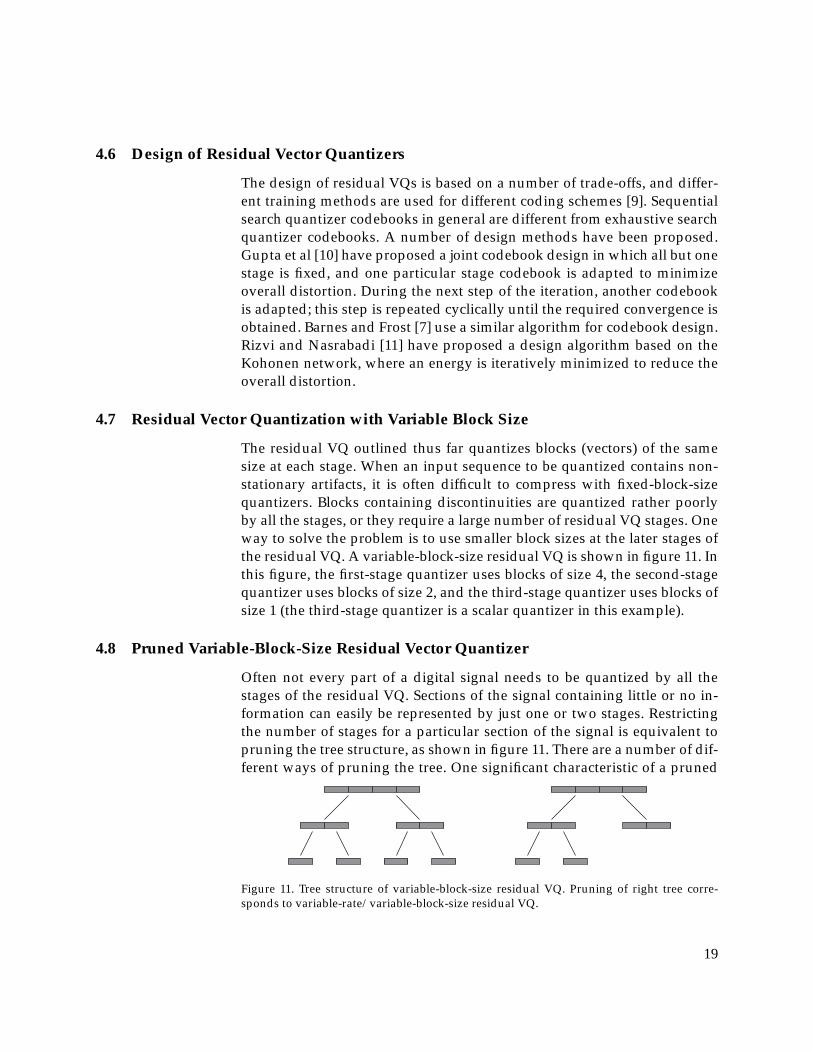
The residual VQ outlined thus far quantizes blocks (vectors) of the samesize at each stage. When an input sequence to be quantized contains non-stationary artifacts, it is often difficult to compress with fixed-block-sizequantizers. Blocks containing discontinuities are quantized rather poorlyby all the stages, or they require a large number of residual VQ stages. Oneway to solve the problem is to use smaller block sizes at the later stages ofthe residual VQ. A variable-block-size residual VQ is shown in figure 11. Inthis figure, the first-stage quantizer uses blocks of size 4, the second-stagequantizer uses blocks of size 2, and the third-stage quantizer uses blocks ofsize 1 (the third-stage quantizer is a scalar quantizer in this example).
4.8 Pruned Variable-Block-Size Residual Vector Quantizer
Often not every part of a digital signal needs to be quantized by all thestages of the residual VQ. Sections of the signal containing little or no in-formation can easily be represented by just one or two stages. Restrictingthe number of stages for a particular section of the signal is equivalent topruning the tree structure, as shown in figure 11. There are a number of dif-ferent ways of pruning the tree. One significant characteristic of a pruned
Figure 11. Tree structure of variable-block-size residual VQ. Pruning of right tree corre-sponds to variable-rate/variable-block-size residual VQ.
19

variable-block-size residual VQ is that very-low-bit-rate side informationneeds to be stored/transmitted. This side information determines the par-ticular tree structure used for every block. The tree structure is required bythe decoder, as it needs to know the number of stages used for every partof the sequence.
4.8.1 Top-Down Pruning Using a Predefined Threshold
This algorithm can decide the number of stages to be used for a particu-lar block by examining the error after every stage. If the error at the endof a particular stage is less than a threshold, then the quantization can bestopped at that stage. The error is measured by a significance measure, suchas the L2 norm (mean squared error). If the L2 distance after stage κ is lessthan a threshold τκ, then quantization is stopped at that stage. Choice ofthe threshold determines the performance of this algorithm. When a singleglobal threshold τ = τ1 = . . . = τk = . . . = τK is used, it directly controlsthe output bit rate of the quantizer.
4.8.2 Optimal Pruning in the Rate-Distortion Sense
Optimal pruning in the rate-distortion sense is a bottom-up pruning tech-nique in which a given block is quantized by all the stages. The quanti-zation error is measured after every stage and stored. For tree pruning,the number of bits required to encode to a particular depth is traded offagainst the distortion. Let T represent a set of all possible tree structuresand QT (X) be the quantized value of X corresponding to the tree structureT . Let L(T ) represent the number of bits required to represent a particulartree structure. For a particular tree structure T , let IT represent the set ofindices after quantization (based on the tree structure) and L(IT ) representthe number of bits required to encode the indices. A Lagrangian formula-tion can be made, and the tree can be pruned according to this objectivefunction. This technique is equivalent to finding a particular tree structurethat minimizes the following cost function:
d(X,Q(X)) + λ · (L(IT ) + L(T )). (12)
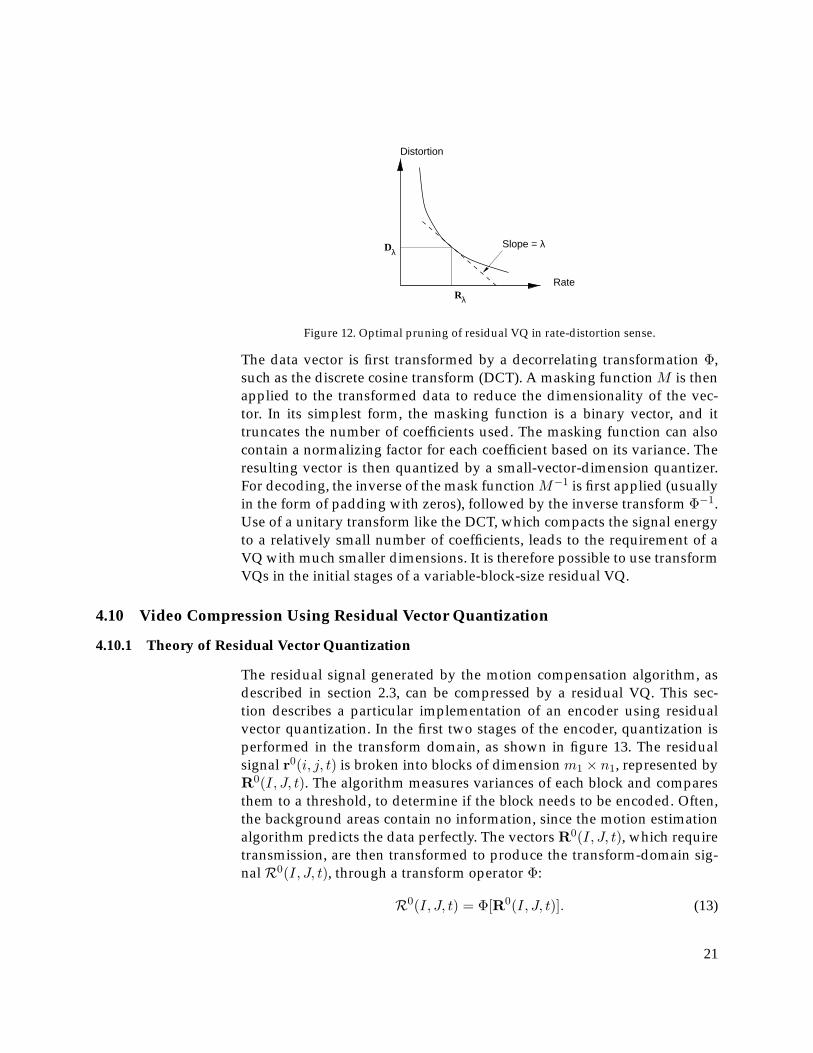
The value of the Lagrangian multiplier λ controls the output bit rate ofthe quantizer. It controls the slope of the tangent to the R-D curve of thequantizer at different operating points, as shown in figure 12.
4.9 Transform-Domain Vector Quantization for Large Blocks
Direct vector quantization of large blocks is computationally expensive,and the design of the codebooks for large-block VQs is difficult. The com-plexity of VQs can be reduced through transform vector quantization [12].
20
Rate
Distortion
Slope = λ
λ
λ
R
D
Figure 12. Optimal pruning of residual VQ in rate-distortion sense.
The data vector is first transformed by a decorrelating transformation Φ,such as the discrete cosine transform (DCT). A masking function M is thenapplied to the transformed data to reduce the dimensionality of the vec-tor. In its simplest form, the masking function is a binary vector, and ittruncates the number of coefficients used. The masking function can alsocontain a normalizing factor for each coefficient based on its variance. Theresulting vector is then quantized by a small-vector-dimension quantizer.For decoding, the inverse of the mask functionM−1 is first applied (usuallyin the form of padding with zeros), followed by the inverse transform Φ−1.Use of a unitary transform like the DCT, which compacts the signal energyto a relatively small number of coefficients, leads to the requirement of aVQ with much smaller dimensions. It is therefore possible to use transformVQs in the initial stages of a variable-block-size residual VQ.
4.10 Video Compression Using Residual Vector Quantization
4.10.1 Theory of Residual Vector Quantization
The residual signal generated by the motion compensation algorithm, asdescribed in section 2.3, can be compressed by a residual VQ. This sec-tion describes a particular implementation of an encoder using residualvector quantization. In the first two stages of the encoder, quantization isperformed in the transform domain, as shown in figure 13. The residualsignal r0(i, j, t) is broken into blocks of dimension m1 × n1, represented byR0(I, J, t). The algorithm measures variances of each block and comparesthem to a threshold, to determine if the block needs to be encoded. Often,the background areas contain no information, since the motion estimationalgorithm predicts the data perfectly. The vectors R0(I, J, t), which requiretransmission, are then transformed to produce the transform-domain sig-nalR0(I, J, t), through a transform operator Φ:
R0(I, J, t) = Φ[R0(I, J, t)]. (13)
21

Motion vectors
Framestore
Σ
DCT IDCT ΣΣ
Variable-length
encoding
Variance andmotion vector based
thresholding
Motion estimation/compensation
Q2
Q3
Q1
Figure 13. Video encoder based on residual vector quantization.
A masking operator M1 is then applied to the transformed vector to pro-duce a truncated vector of reduced dimension, R0
m(I, J, t). This vectorR0m(I, J, t) is quantized by the first-stage VQ. If c1
ι1 is the best matchingcode vector, the approximation of R0(I, J, t) is given by
Q1[R0(I, J, t)] = Φ−1[M−11 (c1
ι1)], (14)
whereM−11 and Φ−1 are the inverses of the masking function and the trans-
form operator. The error after the first-stage quantization is given by
R1(I, J, t) = R0(I, J, t)−Q1[R0(I, J, t)]. (15)
This residual vector is measured for significance, and if it requires furthercompression, a second mask M2 is applied to the transformed vector toproduce vector R1
m(I, J, t). This vector is quantized by the second-stageVQ. If the best match codevector is c2
ι2 , the approximation of R0(I, J, t)after the second stage is given by
Q2[R1(I, J, t)] = Φ−1[M−11 (c1
ι1) +M−12 (c2
ι2)]. (16)
The masking functionsM1 andM2 are binary templates, which together se-lect the first few perceptually significant coefficients. The masking functioneffectively creates a low-pass-filtered version of the signal by discarding thehigher frequency coefficients. The residue after the second stage is given by
R2(I, J, t) = R0(I, J, t)−Q2[R1(I, J, t)]. (17)
22

This residual vector is then split into smaller blocks R′2(I ′, J ′, t) of dimen-sionm2×n2 for quantization by the subsequent stages. The algorithm com-pares the vectors R′2(I ′, J ′, t) with a threshold to determine if they are sig-nificant enough to require transmission. The significant blocks that requiretransmission are quantized by the second-stage VQ, which gives an ap-proximation Q3[R2(I2, J2, t)]. The process of decomposition into smallerblocks and selective quantization is applied recursively in the later stages,so that good representation is obtained of the residual signal r0(i, j, t). Theindices of the quantizers are entropy coded by adaptive arithmetic coding[13].
The block diagram in figure 14 shows that operation of the decoder is notcomplex. The variable-length decoder recovers the bit maps and the code-vector indices from the arithmetically encoded sequence. The decodersare constructed with lookup tables. Based on complexity requirements,the lookup tables of the first two stages can store either the transform-domain coefficients c1
ι1 and c2ι2 or the reconstruction vectors Φ−1[M−1
1 (c1ι1)]
and Φ−1[M−12 (c2
ι2)]. In the first case, two additional operations—a paddingoperation (M−1) and an inverse transform operation (Φ−1)—must be per-formed. In the second case, memory requirements are significantly larger. Ifthe later-stage vectors are required, a direct table lookup is performed, us-ing the indices, and the low-dimension vector is added to the first-stage re-constructed vector in the appropriate position. This process provides the re-constructed residual signal R̂0(I, J, t), which is then passed to the motion-compensation stage to produce the reconstructed frame.
In order to achieve a true variable rate, the encoder makes decisions aboutthe number of quantization stages required by each stage. These decisionshave to be transmitted to the decoder for the encoded data to be decodedcorrectly. The decisions are usually encoded as bit maps for each stage.For a three-stage encoder, three bit maps are required for proper decod-ing. These bit maps could require a significant portion of the bit budget if
Σ
VLC
Motion vectorsMC
IDCT
Σ
Q–1
Q–1
Q–1
Variable-length
decoder
Figure 14. Video decoder based on residual vector quantization.
23
they are not intelligently encoded. The bit map at the first stage is combinedwith the motion vector information so that the number of bits is reduced. Ifthe motion vector of a block is nonzero, it is assumed that the block needsto be encoded by at least the first stage; thus, the overhead first-stage flagbit for blocks with nonzero motion vectors is eliminated. The bit budget forthese bit maps can be further reduced by the use of correlation between thesecond- and third-stage bit maps. Implementation details of an RVQ-basedvideo codec are given by Kwon et al [14].
4.10.2 Performance of an RVQ-Based Video Codec
Simulation results are given for an RVQ-based video encoder with the fol-lowing parameters: the first-stage scalar quantizer (SQ) had 8 quantizationlevels, the codebook size of the second-stage VQ was 16, and the codebooksize of the third-stage VQ was 128. The number of significant DCT coef-ficients used was 9. Simulation results are given for the encoder/decoderoperating at three different very low bit rates. The results are comparedwith those obtained with the H.263 codec [15,16]. For the H.263 codec, allnegotiable options were turned on (except for “PB frames”), so that wecould make a reasonable comparison with the RVQ codec (the PB framemode can be easily incorporated in the RVQ codec). In the H.263 codec,the quantization parameter (QP) for the first frame was set to its maximumvalue, so that the codec would give the best performance for the “intra-frame.” Since we were interested in the steady-state characteristics and notthe first few transient frames, the bits consumed in the first frame were notincluded in the bit-rate calculations. The sequences used were those of thepopular “salesman” test sequence. Each of these sequences has 8-bit pix-els, with frame size 144×176, and the frame rate was 10 frames per second.We evaluated performance by using the peak signal-to-noise ratio (PSNR)measurement to compare the two coding methods. The computation re-quirements for the RVQ codec include real-time DCT; these requirementsare the same as those of H.263. The transform-domain VQ has a codebookof size 16; therefore, its computational complexity is small. Only about 10percent (average over all the sequences tested) of the blocks were encodedby the last VQ stage.
Forty motion-compensated difference frames extracted from four differentsequences (in which the test sequences were not included) were used totrain the codebooks. The codebooks were trained in a three-step process.We first designed the scalar quantizer using the Lloyd’s algorithm. We thengenerated the second- and third-stage initial codebooks using the k-meansalgorithm. Finally, we retrained the three quantizers using the entropy con-straint in a closed-loop manner to improve the rate-distortion performance.
24
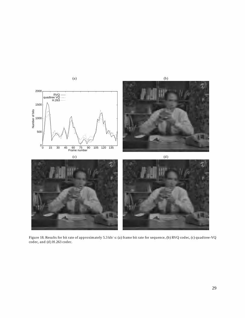
The rate-distortion performance of the two codecs is shown in figure 15(a),which demonstrates that the RVQ codec outperformed H.263 at all threebit rates. At very low bit rates, the PSNR for H.263 decreases drastically,while that of the RVQ codec decreases gradually. The performance on theH.263 codec for the salesman sequence decreases dramatically at very lowbit rates, because of the rather large motion in this sequence. In contrast,the RVQ codec handles such sequences very well at very low bit rates. Fig-ures 15(b), (c), and (d) show the PSNR results of each reconstructed frameat three different bit rates. Since no rate control is used, a variable-bit-rate(VBR) bit stream with constant quality is generated. Figures 16(b), 17(b),and 18(b) show the reconstructed 48th frames for the salesman sequencecompressed at the three different bit rates by the RVQ encoder. Figures16(d), 17(d), and 18(d) show the reconstructed frames compressed by theH.263 encoder at the same bit rates. It can be clearly seen (especially at 5.4kb/s) that H.263 suffers from blocking and smoothing, while the output ofthe RVQ codec is of much better visual quality.
25

(a) (b)
30
30.5
31
31.5
32
32.5
33
33.5
5 6 7 8 9 10 11 12 13
Dis
tort
ion
(dB
)
Bit rate (kb/s)
RVQquadtree VQ
H.263
28
29
30
31
32
33
34
35
36
0 15 30 45 60 75 90 105 120 135 150
PS
NR
(dB
)
Frame number
RVQquadtree VQ
H.263
(c) (d)
28
29
30
31
32
33
34
35
0 15 30 45 60 75 90 105 120 135
PS
NR
(dB
)
Frame number
RVQquadtree VQ
H.263
27
28
29
30
31
32
33
34
0 15 30 45 60 75 90 105 120 135
PS
NR
(dB
)
Frame number
RVQquadtree VQ
H.263
Figure 15. Performance of video compression algorithms using vector quantization: (a) rate-distortion performance,(b) PSNR results at 12 kb/s, (c) PSNR results at 8.1 kb/s, and (d) PSNR results at 5.3 kb/s.
26

(a) (b)
0
500
1000
1500
2000
2500
3000
3500
4000
0 15 30 45 60 75 90 105 120 135
Num
ber
of b
its
Frame number
RVQquadtree VQ
H.263
(c) (d)
Figure 16. Results for bit rate of approximately 12 kb/s: (a) frame bit rate for sequence, (b) RVQ codec, (c) quadtree-VQcodec, and (d) H.263 codec.
27

(a) (b)
0
500
1000
1500
2000
2500
3000
0 15 30 45 60 75 90 105 120 135
Num
ber
of b
its
Frame number
RVQquadtree VQ
H.263
(c) (d)
Figure 17. Results for bit rate of approximately 8.1 kb/s: (a) frame bit rate for sequence, (b) RVQ codec, (c) quadtree-VQcodec, and (d) H.263 codec.
28
(a) (b)
0
500
1000
1500
2000
0 15 30 45 60 75 90 105 120 135
Num
ber
of b
its
Frame number
RVQquadtree VQ
H.263
(c) (d)
Figure 18. Results for bit rate of approximately 5.3 kb/s: (a) frame bit rate for sequence, (b) RVQ codec, (c) quadtree-VQcodec, and (d) H.263 codec.
29

5. Quadtree-Based Vector Quantization
A quadtree is a hierarchical data structure used to represent regions,curves, surfaces, and volumes. Representations of regions by a quadtreeare achieved by the successive subdivision of the image array into fourequal quadrants. This process is known as a regular decomposition of anarray. An image is thus decomposed into homogeneous regions with sidesof lengths that are powers of two. A tree of degree 4 (each nonleaf hasfour children) is generated to represent the image in terms of its homo-geneous regions. The root node corresponds to the entire array, and eachchild of a node represents a quadrant of the region represented by thatnode. Leaf nodes of the tree correspond to those blocks for which no furthersubdivision is necessary. The above segmentation procedure is known as atop-down construction of the quadtree. Another possibility for construct-ing a quadtree is a bottom-up procedure, where small blocks are mergedtogether recursively to form a larger block if they are homogeneous withrespect to the merging criterion.
The regular decomposition method does not necessarily correspond to thesegmentation of the image into maximal homogeneous regions. It is likelythat unions of adjacent blocks form homogeneous regions. To obtain thesemaximal homogeneous regions, we must allow the merging of adjacentblocks. However, the resulting partition will no longer be represented bya quadtree; instead, the final representation is in the form of an adjacencygraph. (An alternative method to obtain maximal homogeneous regions isto use a decomposition technique that is not regular: that is, it segmentsthe image into rectangular blocks of arbitrary size. Such a method wouldrequire a different coding procedure for each block size.) Here, we use aregular decomposition method because the resulting blocks are square; thismethod reduces the complexity of the encoder, the decoder, and the num-ber of bits required to represent the binary quadtree. The homogeneousregions so obtained are thus not necessarily maximal.
5.1 Quadtree Decomposition
A quadtree decomposition results in an unbalanced tree structure with leafnodes of different sizes. In a regular decomposition, the leaf nodes are re-stricted to square blocks. It is further possible to restrict the sides of theleaf nodes to a small range of values. Such a restriction results in a tree
30
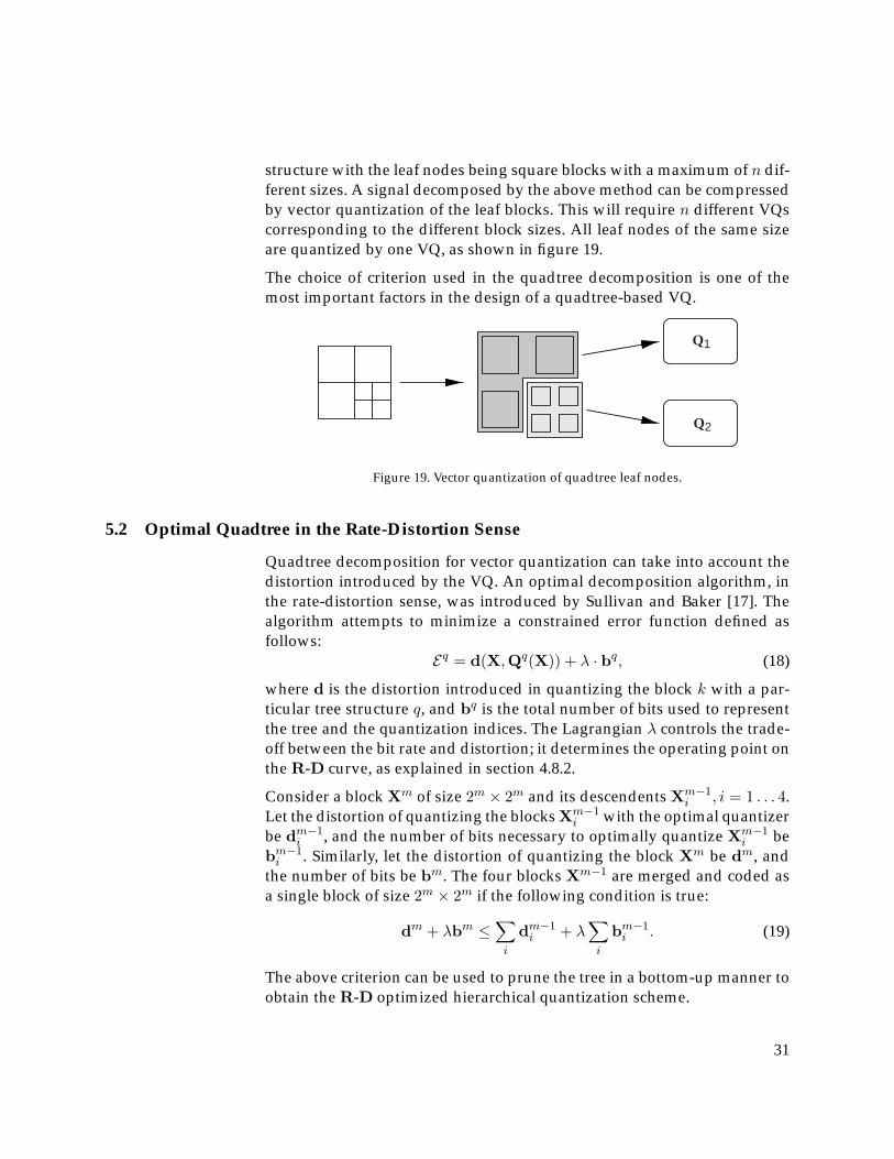
structure with the leaf nodes being square blocks with a maximum of n dif-ferent sizes. A signal decomposed by the above method can be compressedby vector quantization of the leaf blocks. This will require n different VQscorresponding to the different block sizes. All leaf nodes of the same sizeare quantized by one VQ, as shown in figure 19.
The choice of criterion used in the quadtree decomposition is one of themost important factors in the design of a quadtree-based VQ.
Q1
Q2
Figure 19. Vector quantization of quadtree leaf nodes.
5.2 Optimal Quadtree in the Rate-Distortion Sense
Quadtree decomposition for vector quantization can take into account thedistortion introduced by the VQ. An optimal decomposition algorithm, inthe rate-distortion sense, was introduced by Sullivan and Baker [17]. Thealgorithm attempts to minimize a constrained error function defined asfollows:
Eq = d(X,Qq(X)) + λ · bq, (18)
where d is the distortion introduced in quantizing the block k with a par-ticular tree structure q, and bq is the total number of bits used to representthe tree and the quantization indices. The Lagrangian λ controls the trade-off between the bit rate and distortion; it determines the operating point onthe R-D curve, as explained in section 4.8.2.
Consider a block Xm of size 2m × 2m and its descendents Xm−1i , i = 1 . . . 4.
Let the distortion of quantizing the blocks Xm−1i with the optimal quantizer
be dm−1i , and the number of bits necessary to optimally quantize Xm−1
i bebm−1i . Similarly, let the distortion of quantizing the block Xm be dm, and
the number of bits be bm. The four blocks Xm−1 are merged and coded asa single block of size 2m × 2m if the following condition is true:
dm + λbm ≤∑i
dm−1i + λ
∑i
bm−1i . (19)
The above criterion can be used to prune the tree in a bottom-up manner toobtain the R-D optimized hierarchical quantization scheme.
31

5.3 Video Compression Using Quadtree-Based Vector Quantization
The residual signal generated by the motion-compensation algorithm canbe compressed by the quadtree VQ [18]. The residual signal r0(i, j, t) is di-vided into blocks of size 2m×2m. Each of these blocks is encoded by the R-D optimized, quadtree-based VQs. A k-stage hierarchical VQ uses k VQs,which work blocks of size 2n × 2n, n = m, . . . ,m− k. The quadtree bitmapis encoded as shown in figure 20.
We have implemented a video compression system using the quadtree VQthat we describe here. A simulation framework similar to that used in theRVQ video codec was used in evaluating the performance of the quadtree-VQ-based video compression algorithm. The residual signal after motioncompensation was compressed by a three-stage quadtree VQ. The threequantizers used blocks of size 16×16, 8×8, and 4×4, respectively. Resultsare given for an encoder that uses scalar quantizers for blocks of size 16×16and 8×8. Blocks of 4×4 are compressed by a VQ trained by the GLA algo-rithm. The quadtree was segmented with the R-D optimized algorithm. Wetested the performance using the “salesman” sequence at three very low bitrates, as we did for the motion-compensated RVQ video codec. The perfor-mance of the quadtree-VQ compression algorithm was numerically similarto that of the RVQ compression algorithm. Figure 15 shows the PSNR re-sults of each reconstructed frame at three different bit rates. Figures 16c,17c, and 18c show the reconstructed 48th frames for the salesman sequencecompressed at the three different bit rates by the quadtree-VQ encoder. Asthese figures show, the performance of the quadtree-VQ encoder is similarto that of the RVQ encoder at all the bit rates.
43
21
4321
Code: 1( 1(0010) 0 1(1000) 1(1000) )
Figure 20. Encoding quadtree data structure.
32
6. Conclusions
In this report, we have explored two vector-quantization-based video com-pression algorithms. In our work we have identified two important areasthat can be exploited to improve upon existing coding methods:
1. Multiscale segmentation: different areas in the image are coded at dif-ferent scales. In vector quantization, this is equivalent to using differ-ent block sizes for different areas.
2. Multirate coding: different areas in the image are coded at differ-ent precisions, since all areas of the image do not contain the sameamount of information.
We have used two different methods to achieve the above goals. In theRVQ-based encoder, we use the successive-refinement paradigm to achievea variable rate. In the quadtree-VQ encoder, the rate variability is limited,but this technique is superior to a successive-refinement technique becauseit performs direct quantization. Both algorithms use variable block sizes.The resulting performance of these two encoders is similar, and both typesare superior to existing video compression standards.
33
References
1. Y. Linde, A. Buzo, and R. M. Gray. An algorithm for vector quantizerdesign. IEEE Trans. Commun., 28(1):84–95, January 1980.
2. T. Kohonen. Self-Organization and Associative Memory. Springer-Verlag,1984.
3. N. M. Nasrabadi and Y. Feng. Vector quantization of images basedupon the Kohonen self-organization feature maps. International Con-ference on Neural Networks, I:101–105, 1988.
4. P. A. Chou, T. Lookabaugh, and R. M. Gray. Entropy-constrained vec-tor quantization. IEEE Trans. Acoust. Speech Signal Process., 37(1), Jan-uary 1989.
5. S. Roucos, J. Makhoul, and H. Gish. Vector quantization in speech cod-ing. Proc. IEEE, 73(11):1551–1587, November 1985.
6. B. H. Juang and A. H. Gray. Multiple stage vector quantization forspeech coding. Proc. IEEE ICASSP, 1:597–600, April 1982.
7. C. F. Barnes and R. L. Frost. Vector quantizers with direct sum code-books. IEEE Trans. Info. Theory, 39(2):565–580, March 1993.
8. W.H.R. Equitz and T. M. Cover. Successive refinement of information.IEEE Trans. Inf. Theory, 37(2):269–275, March 1991.
9. C. F. Barnes, S. A. Rizvi, and N. M. Nasrabadi. Advances in residualvector quantization: A review. IEEE Trans. Image Process., 5(2), Febru-ary 1996.
10. S. Gupta, W. Y. Chan, and A. Gersho. Enhanced multistage vec-tor quantizer by joint codebook design. IEEE Trans. Commun.,40(11):1693–1697, November 1992.
11. S. A. Rizvi and N. M. Nasrabadi. Residual vector quantization usinga multi-layer competitive neural network. IEEE J. Selected Areas Com-mun., 12(9):1452–1459, December 1994.
34
12. R. A. King and N. M. Nasrabadi. Image coding using vector quan-tization in the transform domain. Pattern Recognition Lett., 1:323–329,1983.
13. I. H. Witten, R. M. Neal, and J. G. Cleary. Arithmetic coding for datacompression. Commun. ACM, 30(6):520–540, June 1987.
14. H. Kwon, M. Venkatraman, and N. M. Nasrabadi. Very low bit-ratevideo coding using variable block-size entropy-constrained residualvector quantizers. IEEE J. Selected Areas Commun., 15(9):1714–1725,December 1997.
15. K. N. Ngan, D. Chai, and A. Millin. Very low bit rate video codingusing H.263 coder. IEEE Trans. Circuits Syst. Video Technol., 6(3):308–312, June 1996.
16. Telenor R&D. TMN (H.263) encoder/decoder, ftp://bonde.nta.no/pub/tmn. TMN codec, May 1996.
17. G. J. Sullivan and R. L. Baker. Efficient quadtree coding of images andvideo. IEEE Trans. Image Process., 3(3):327–331, May 1994.
18. N. M. Nasrabadi, S. Lin, and Y. Feng. Interframe hierarchical vectorquantization. Opt. Engineer., 28(7):717–725, July 1989.
35
37
Distribution
AdmnstrDefns Techl Info CtrAttn DTIC-OCP8725 John J Kingman Rd Ste 0944FT Belvoir VA 22060-6218
Ofc of the Dir Rsrch and EngrgAttn R MenzPentagon Rm 3E1089Washington DC 20301-3080
Ofc of the Secy of DefnsAttn ODDRE (R&AT) G SingleyAttn ODDRE (R&AT) S GontarekThe PentagonWashington DC 20301-3080
OSDAttn OUSD(A&T)/ODDDR&E(R) R TruWashington DC 20301-7100
CECOMAttn PM GPS COL S YoungFT Monmouth NJ 07703
CECOMSp & Terrestrial Commctn DivAttn AMSEL-RD-ST-MC-M H SoicherFT Monmouth NJ 07703-5203
Dept of the Army (OASA) RDAAttn SARD-PT R Saunders103 ArmyWashington DC 20301-0103
Dir for MANPRINTOfc of the Deputy Chief of Staff for PrsnnlAttn J HillerThe Pentagon Rm 2C733Washington DC 20301-0300
Hdqtrs Dept of the ArmyAttn DAMO-FDT D Schmidt400 Army Pentagon Rm 3C514Washington DC 20301-0460
MICOM RDECAttn AMSMI-RD W C McCorkleRedstone Arsenal AL 35898-5240
US Army ATCOMAttn AMSAC-R-TD-CC R WallFT Eustis VA 23604-1104
US Army CECOMAttn AMSEL-RD-C3-AC P SassFT Monmouth NJ 07703
US Army CECOMAttn AVESD GardD IIFT Belvoir VA 22060-5806
US Army CECOM Rsrch, Dev, & Engrg CtrAttn R F GiordanoFT Monmouth NJ 07703-5201
Night Vsn & Elect Sensors DirctrtUS Army Commctn-Elect CmndAttn T Jones10221 Burbeck Rd Ste 430FT Belvoir VA 22060-5806
US Army Edgewood Rsrch, Dev, & Engrg CtrAttn SCBRD-TD J VervierAberdeen Proving Ground MD 21010-5423
US Army Info Sys Engrg CmndAttn ASQB-OTD F JeniaFT Huachuca AZ 85613-5300
US Army Materiel Sys Analysis AgencyAttn AMXSY-D J McCarthyAberdeen Proving Ground MD 21005-5071
US Army Matl CmndDpty CG for RDE HdqtrsAttn AMCRD BG Beauchamp5001 Eisenhower AveAlexandria VA 22333-0001
US Army Matl Cmnd PrinDpty for Acquisition HdqrtsAttn AMCDCG-A D Adams5001 Eisenhower AveAlexandria VA 22333-0001

Distribution (cont’d)
38
US Army Matl CmndPrin Dpty for Techlgy HdqrtsAttn AMCDCG-T M Fisette5001 Eisenhower AveAlexandria VA 22333-0001
US Army Natick Rsrch, Dev, & Engrg CtActing Techl DirAttn SSCNC-T P BrandlerNatick MA 01760-5002
US Army Rsrch OfcAttn AMXRO-EL W SanderPO Box 12211Research Triangle Park NC 22709-2211
US Army Rsrch OfcAttn G Iafrate4300 S Miami BlvdResearch Triangle Park NC 27709
US Army Simulation, Train, & InstrmntnCmnd
Attn J Stahl12350 Research ParkwayOrlando FL 32826-3726
US Army TACOMAttn AMSTA-TA-D P Hanjack MS 201BAttn AMSTA-TR-R K Adams MS 264Warren MI 48397
US Army Tank-Automtv & Armaments CmndAttn AMSTA-AR-TD C SpinelliBldg 1Picatinny Arsenal NJ 07806-5000
US Army Tank-Automtv Cmnd Rsrch, Dev, &Engrg Ctr
Attn AMSTA-TA J ChapinWarren MI 48397-5000
US Army Test & Eval CmndAttn R G Pollard IIIAberdeen Proving Ground MD 21005-5055
US Army Train & Doctrine CmndBattle Lab Integration & Techl DirctrtAttn ATCD-B J A KleveczFT Monroe VA 23651-5850
US Military AcademyDept of Mathematical SciAttn MAJ D EngenWest Point NY 10996
Nav Air Warfare CtrAttn S Gattis1 Admin CircleChina Lake CA 93555-6001
DirNav Rsrch LabWashington DC 20375-5000
Nav Surface Warfare CtrAttn Code B07 J Pennella17320 Dahlgren Rd Bldg 1470 Rm 1101Dahlgren VA 22448-5100
ComdtUS Nav AcademyAnnapolis MD 21404
GPS Joint Prog Ofc DirAttn COL J Clay2435 Vela Way Ste 1613Los Angeles AFB CA 90245-5500
ComdtUS AF AcademyColorado Springs CO 80840
DARPAAttn B KasparAttn L Stotts3701 N Fairfax DrArlington VA 22203-1714
ARL Electromag GroupAttn Campus Mail Code F0250 A TuckerUniversity of TexasAustin TX 78712
Univ of Delaware Dept of Elect EngrgAttn C Boncelet JrNewark DE 19716
Ericsson Inc Adv Dev & Rsrch GrpAttn A KhayrallahResearch Triangle Park NC 27709

39
Distribution (cont’d)
ERIMAttn J Ackenhusen1975 Green RdAnn Arbor MI 48105
Natl Inst Standards/TechAttn J PhillipsBldg 225 Rm A216Gaithersburg MD 20899
Sanders Lockheed Martin CoAttn PTP2-A001 K DamourPO Box 868Nashua NH 03061-0868
US Army Rsrch LabAttn AMSRL-IS-C R KasteAberdeen Proving Ground MD 21005
US Army Rsrch LabAttn AMSRL-IS-CS A MarkAttn AMSRL-CI-AC AngelniAberdeen Proving Ground MD 21005-5055
US Army Rsrch LabAttn AMSRL-CI-LL Techl Lib (3 copies)Attn AMSRL-CS-AL-TA Mail & Records
MgmtAttn AMSRL-CS-AL-TP Techl Pub (3 copies)Attn AMSRL-IS P EmmermanAttn AMSRL-IS R SlifeAttn AMSRL-IS-CI B BroomeAttn AMSRL-IS-CI T MillsAttn AMSRL-IS-TA J GowensAttn AMSRL-IS-TP A BrodeenAttn AMSRL-IS-TP A Downs
US Army Rsrch Lab (cont’d)Attn AMSRL-IS-TP B CooperAttn AMSRL-IS-TP C SarafidisAttn AMSRL-IS-TP D GwynAttn AMSRL-IS-TP D TorrieriAttn AMSRL-IS-TP F BrundickAttn AMSRL-IS-TP G CirincioneAttn AMSRL-IS-TP G HartwigAttn AMSRL-IS-TP H CatonAttn AMSRL-IS-TP L WrencherAttn AMSRL-IS-TP M LopezAttn AMSRL-IS-TP M MarkowskiAttn AMSRL-IS-TP M RetterAttn AMSRL-IS-TP S ChamberlainAttn AMSRL-SC-I A RaglinAttn AMSRL-SC-I T HanrattyAttn AMSRL-SC-SA WallAttn AMSRL-SE J M MillerAttn AMSRL-SE J PellegrinoAttn AMSRL-SE-EE Z G SztankayAttn AMSRL-SE-SE D NguyenAttn AMSRL-SE-SE H KwonAttn AMSRL-SE-SE L BennettAttn AMSRL-SE-SE M Venkatraman
(5 copies)Attn AMSRL-SE-SE M VrabelAttn AMSRL-SE-SE N NasrabadiAttn AMSRL-SE-SE P RaussAttn AMSRL-SE-SE S DerAttn AMSRL-SE-SE T KippAttn AMSRL-SE-SR A M P MarinelliAttn AMSRL-SE-SS V MarinelliAdelphi MD 20783-1197

1. AGENCY USE ONLY
8. PERFORMING ORGANIZATION REPORT NUMBER
7. PERFORMING ORGANIZATION NAME(S) AND ADDRESS(ES)
12a. DISTRIBUTION/AVAILABILITY STATEMENT
10. SPONSORING/MONITORING AGENCY REPORT NUMBER
5. FUNDING NUMBERS4. TITLE AND SUBTITLE
6. AUTHOR(S)
REPORT DOCUMENTATION PAGE
3. REPORT TYPE AND DATES COVERED2. REPORT DATE
11. SUPPLEMENTARY NOTES
14. SUBJECT TERMS
13. ABSTRACT (Maximum 200 words)
Form ApprovedOMB No. 0704-0188
(Leave blank)
9. SPONSORING/MONITORING AGENCY NAME(S) AND ADDRESS(ES)
Public reporting burden for this collection of information is estimated to average 1 hour per response, including the time for reviewing instructions, searching existing data sources,gathering and maintaining the data needed, and completing and reviewing the collection of information. Send comments regarding this burden estimate or any other aspect of thiscollection of information, including suggestions for reducing this burden, to Washington Headquarters Services, Directorate for Information Operations and Reports, 1215 JeffersonDavis Highway, Suite 1204, Arlington, VA 22202-4302, and to the Office of Management and Budget, Paperwork Reduction Project (0704-0188), Washington, DC 20503.
12b. DISTRIBUTION CODE
15. NUMBER OF PAGES
16. PRICE CODE
17. SECURITY CLASSIFICATION OF REPORT
18. SECURITY CLASSIFICATION OF THIS PAGE
19. SECURITY CLASSIFICATION OF ABSTRACT
20. LIMITATION OF ABSTRACT
NSN 7540-01-280-5500 Standard Form 298 (Rev. 2-89)Prescribed by ANSI Std. Z39-18298-102
Unclassified
ARL-TR-1535
Interim, May 1997 to July 1997May 1998
PE: 61102A
47
Video Compression using Vector Quantization
Mahesh Venkatraman, Heesung Kwon, and Nasser M. Nasrabadi
U.S. Army Research LaboratoryAttn: AMSRL-SE-SE (e-mail: [email protected])2800 Powder Mill RoadAdelphi, MD 20783-1197
U.S. Army Research Laboratory2800 Powder Mill RoadAdelphi, MD 20783-1197
Approved for public release; distribution unlimited.
AMS code: 611102.305ARL PR: 7NE0M1
This report presents some results and findings of our work on very-low-bit-rate video compressionsystems using vector quantization (VQ). We have identified multiscale segmentation and variable-ratecoding as two important concepts whose effective use can lead to superior compression performance.Two VQ algorithms that attempt to use these two aspects are presented: one based on residual vectorquantization and the other on quadtree vector quantization. Residual vector quantization is a succes-sive approximation quantizer technique and is ideal for variable-rate coding. Quadtree vectorquantization is inherently a multiscale coding method. The report presents the general theoreticalformulation of these algorithms, as well as quantitative performance of sample implementations.
Motion estimation, residual VQ, quadtree VQ
Unclassified Unclassified UL
41
DEP
AR
TMEN
T O
F TH
E A
RM
YA
n E
qual
Opp
ortu
nity
Em
ploy
erU
.S. A
rmy
Res
earc
h La
bora
tory
2800
Pow
der
Mill
Roa
dA
delp
hi, M
D 2
0783
-119
7