How Do Indian Voters Respond to Candidates with Criminal Charges : Evidence from the 2009 Lok Sabha Elections

Bhaskar Dutta and Poonam Gupta1

July 2012

Abstract

This paper examines the response of voters to candidates who have reported that they have criminal charges against them, within the framework of a simple analytical model which assumes that criminal charges give rise to some stigma amongst the electorate, and result in a negative effect on vote shares. Campaigning, the cost of which is borne from candidates’ wealth, helps a candidate to increase his or her expected vote share by winning over the “marginal” voter. A criminal candidate gets an additional benefit since he can use the campaigning to convince voters of his innocence, and so reduce the negative effects of the stigma associated with criminal charges. We test the implications of the model using data for the 2009 Lok Sabha elections in India, and find support for all the implications of the model. Our empirical results show that voters do penalise candidates with criminal charges; however, this negative effect is reduced if there are other candidates in the constituency with criminal charges; besides, the vote shares are positively related to candidate wealth, with the marginal effect being higher for the candidates with criminal charges.

1 University of Warwick and National Institute of Public Finance and Policy, Delhi, respectively. We thank Honey Karun for excellent research assistance. Comments are welcome at B.Dutta@warwick.ac.uk and pgupta.nipfp@gmail.com. We are very grateful to Wiji Arulampalam, Rajeev Dehejia, Sugato Dasgupta, Lakshmi Iyer and K.L. Krishna for comments and helpful suggestions.

1

1. Introduction

It is now well-known that the nexus between Indian politicians and criminals has assumed

alarming proportions. Roughly a fourth of the members of the current Lok Sabha (the lower

house of the national parliament) face pending criminal charges.2 A similar situation prevails in

the various state assemblies. Many of the members of the national parliament or states

assemblies have been indicted with serious charges including murder. Not surprisingly, this has

attracted increasing attention in both the media as well as in academic research. It has also

attracted official attention with the appointment of an independent commission to analyse the

phenomenon and suggest remedial measures.3

It would be misleading to suggest that there is a complete absence of legal measures to

prevent the influx of criminals into parliament and the state assemblies. In fact, the

Representation of People’s Act, 1951 specifies that candidates will be barred from contesting an

election on conviction by a court of Law. The period of disqualification is for six years from the

date of conviction, or from the date of release from prison, depending on the severity of the

charge. Unfortunately, this law hardly has any bite because of the well-known infirmities in the

Indian judicial system. In particular, governments typically drag their feet when it comes to

prosecuting “local elites”. Even when cases are registered, inordinate judicial delay implies that

these cases drag on, seemingly indefinitely.

This is why the Election Commission had proposed in 2004 that the Representation of the

People Act, 1951 should be amended to disqualify candidates accused of offences which carry

sentences of five years or more as soon as a court deems that charges can be framed against the

person. However, the Lok Sabha itself would be required to pass appropriate legislation to

implement the Election Commission’s suggestion. Obviously, such legislation is against the

interests of a large number of politicians, and so it is not surprising that the Election

Commission’s proposal has not been implemented.

A landmark judgement of the Supreme Court in 2002 required every candidate contesting

state and national elections to submit a legal affidavit disclosing his or her personal educational

qualifications, as well as information about personal wealth and importantly their criminal

2 That is, courts have decided that these charges have sufficient credibility for judicial proceedings to be initiated. However, this does not mean that these charges have culminated in convictions.3 See the Vohra Commission Report, 1995.

2

record. The court also stipulated that wide publicity should be given to the contents of the

affidavits so that the electorate can take an informed decision about who to elect to the

assemblies and parliaments. Unfortunately, the Supreme Court’s order does not seem to have had

much impact in so far as the influx of legislators with criminal indictment is concerned.4

The continuing entry of large numbers of candidates with criminal records into Indian

legislatures raises several questions. First, why do parties nominate such candidates? Given the

huge demand for party tickets, the nomination of candidates with criminal records suggests that

such candidates must possess some electoral advantage. We discuss some hypotheses which

have been suggested to explain this electoral advantage. Second, what is the economic effect of

electing candidates with a criminal record? Third, what is the response of voters to candidates

who have reported that they have criminal charges against them?

While the first two issues have been discussed in the literature, the third issue has not

been scrutinised rigorously. A somewhat cursory look at the data by simply looking at the ratio

of winning candidates to number of contesting candidates amongst the criminal and non-criminal

groups suggests that criminal candidates have a higher probability of winning. Perhaps, this has

given rise to the feeling that criminals have an electoral advantage. The following from Aidt et al

(2011) is representative of the prevailing view: “Criminals, we show, boast an extraordinary

electoral advantage in India.”

We examine this issue within the framework of an analytical model which assumes that

criminal charges do give rise to some stigma amongst the electorate. This stigma has a negative

effect on vote shares since voters are less likely to vote for candidates who have criminal charges

levied against them. Campaigning, the cost of which is borne from candidates’ wealth, helps a

candidate to increase his or her expected vote share by winning over the “marginal” voter. A

criminal candidate gets an additional benefit since he can use the campaigning to convince voters

of his innocence, and so reduce the negative effects of the stigma associated with criminal

charges. This is plausible since the candidates have not been convicted, but only charged with

some criminal offence. We look at a Nash equilibrium of a game in which the only strategic

variable is the amount of campaign expenditure.

4 However, the judgement has been of immense help to several researchers who have exploited the information contained in the affidavits. Apart from the present paper, see, for instance, Aidt et al (2011), Chemin (2008), Paul and Vivekananda (2004), Vaishnav (2011).

3

We test the implications of this simple model using data for the 2009 Lok Sabha

elections. We find that the data supports all the implications of the model. We briefly describe

the principal results.

First, voters do penalise candidates with criminal charges. That is, all else being equal,

the vote share of a candidate with criminal charges is lower than that of the one who does not

have any such blemish. However, this negative effect is reduced if there are other candidates in

the constituency with criminal charges. Notice that the negative effect of criminal charges on

vote shares seems to contradict the prevalent view that candidates with criminal charges have an

electoral advantage.

We do not have data on campaign expenditure of candidates. However, our model

predicts that (i) the higher the wealth of a candidate, the greater will be his campaign

expenditure, (ii) campaign expenditure has a positive effect on expected vote share, the marginal

effect possibly differing across the two categories of candidates - those with criminal charges,

and those with an unblemished record. Putting these together, the model prediction is that

expected vote shares should be positively related to candidate wealth, with the marginal effect

perhaps being different across the two categories of candidates. The regression results

corroborate both conclusions.

Since voters penalise candidates with criminal charges, why do political parties still

nominate them when so many candidates without criminal charges fight to get their party’s

nomination? A plausible explanation starts from the premise that candidates facing the threat of

criminal convictions are more keen to contest the elections. Their enthusiasm is easily explained.

Apart from the usual benefits which accrue to all successful candidates, candidates with criminal

indictments look forward to an additional benefit. In particular, successful candidates

(particularly those belonging to parties in the government) can with high probability either use

coercion or influence to ensure that the local administration does not pursue the case(s) against

them with any vigour.

Moreover, the data suggest that criminal candidates are wealthier than those without

criminal charges.5 Also, they are probably willing to contribute a higher fraction of their wealth

to the party, or perhaps they ask for less resources from the party. This simply reflects the higher

price or value that they place on a party ticket. So, criminal candidates generate positive

5 Vaishnav (2011) also finds that potentially criminal candidates have higher wealth.

4

externalities to candidates of their own party since their additional contributions release party

funds which can be used in other constituencies. This explains why parties may nominate

candidates with criminal backgrounds even if they are (partially) penalised at the polls.

Several recent papers offer explanations of why parties choose candidates with a dubious

background. Banerjee and Pande (2009) start with the observation that voters may have a

preference for candidates belonging to their own ethnic group. This implies that a politician

belonging to the ethnically dominant group in a constituency may win even if he is of lower

quality. Banerjee and Pande (2009) assume that parties do want to select candidates of the best

quality. However, the quality of candidates available to a party in any constituency is a random

variable. They show that an increase in the relative size of the ethnically dominant group or an

increase in voters’ preferences for candidates belonging to their own group can worsen the

quality of the winning candidate. Banerjee and Pande test the predictions of their model by using

panel data on politician quality in 102 jurisdictions in the state of Uttar Pradesh.6

Of course, the Banerjee-Pande hypothesis does not explain why so many candidates with

a criminal background contest elections. But, it does provide at least a partial explanation of why

there is an increasing number of successful legislators in state assemblies as well as the Lok

Sabha with criminal background.

Vaishnav (2011) studies elections to 28 state assemblies between 2003 and 2009. He

finds that personal wealth of candidates is positively associated with criminal status where a

candidate is defined to be a criminal if he has been charged with a “serious” crime. The basic

result is subjected to a variety of robustness checks. This leads him to offer the same explanation

that we have mentioned earlier - parties nominate criminal candidates simply because they

contribute larger sums to the party coffers.

Aidt. el al (2011) develop an interesting theoretical model where they assume that

criminal candidates have some electoral advantage, although parties also incur some reputational

cost in nominating them. They “are agnostic about the sources of this advantage”, but speculate

that the electoral advantage of criminals could arise because they can intimidate prospective

voters of rival parties into staying away from the polls. Notice that this would imply voting

turnout should be negatively correlated with number of criminals in a constituency. We show

that this is not true in the 2009 Lok Sabha elections.

6 They measure a politician’s quality by his record of illegal and corrupt behaviour as identified in a field survey.

5

So, parties face a trade-off between the reputational cost of nominating candidates with

criminal charges and their electoral advantage. This trade-off implies that parties would be more

willing to incur the reputational cost in constituencies which are likely to witness close contests

since the electoral advantage is more attractive in these constituencies. Conversely, a party

would be unlikely to field a tainted candidate in a constituency where the party is very likely to

win. Similarly, candidates with criminal indictments are more likely to be fielded in

constituencies where the cost is lower – for instance, in constituencies where voters are poorly

informed about the characteristics of the contesting candidates.

These theoretical predictions are plausible enough given the specified model.

Unfortunately, there are some questionable issues in their empirical exercise. Perhaps, the most

problematic is that they use literacy as the proxy for the cost of fielding a tainted candidate. Their

rationale for doing so is that illiterate voters are less likely to be aware of the criminal

background of the contesting candidates. Even if this is accepted at face value, there are at least

two problems with using literacy as an explanatory variable. First, the only available data on

literacy is from the 2001 Census, although their electoral data are for the 2004 and 2009 Lok

Sabha elections. Second, census data are available only for administrative districts which do not

coincide with political constituencies. Clearly, literacy data at the constituency level for 2004

and 2009 simply do not exist!

Aidt et al measure competitiveness by the percentage difference between the vote shares

of the winning candidate and her closest rival in the same election. This raises serious

endogeneity problems since the individual candidate characteristics (whether of criminal

background or not) presumably has some influence on vote shares and hence on the measure of

competitiveness used by the authors!

Chemin (2008) studies state elections and observes that bureaucratic corruption is lower

in constituencies which elect criminal representatives. He also finds that poverty is higher in

these constituencies. However, the mechanisms through which these effects operate is not spelt

out in any detail.

The rest of the paper is organized as follows. In section 2 the theoretical framework is

laid out and the testable hypotheses are spelt out. The econometric specification and the details

6

on the data and the different data sources used in the paper are described in section 3. Results

from the empirical exercise are discussed in section 4, and the last section concludes.

2. The Theoretical Framework

In this section, we outline a simple model of electoral competition which provides a

rationalization for the regression equation(s) that we use in the paper. Before setting out the

formal model, we briefly outline its basic features. Fix any constituency. Since we want to focus

on how criminal charges affect the electoral fortunes of different candidates in the constituency,

we do not consider how candidates choose their policy platforms. Instead, we assume that every

candidate i in the constituency has a fixed policy or electoral platform. An alternative

interpretation is that policy platforms are chosen in the first stage. Given the vector of policy

platforms, candidates decide how much to spend on campaigning in the second stage. The main

focus of the theoretical model is on how candidates decide on the amount of campaign

expenditure, and how this affects expected vote shares.

Voters take into account the vector of policy platforms as well as candidate

characteristics such as education, their past record in public service and party characteristics in

deciding which candidate to support. A particular candidate characteristic that we will emphasize

in the paper is criminal record. That is, some candidates may have a certain number of criminal

charges levied against them. Such criminal charges result in some stigma associated to the

candidates.7

Campaign expenditures benefit candidates in two ways. First, campaigning helps each

candidate to influence voters that his or her electoral platform and individual characteristics are

superior to that of the rivals. Second, candidates with criminal charges can campaign to

convince voters that the charges leveled against them are baseless.8 Voters base their voting

decisions on the policy platforms, and candidate characteristics including the stigma attached to

the different candidates. Finally, candidates choose the amount of campaign expenditure taking

into account their expected vote share and its cost.

7 We use the term “stigma” to refer to the negative feeling experienced by voters about the candidate. All other things being equal, voters will prefer to vote for the candidate with a lower level of stigma.8 There is anecdotal evidence that in several states, candidates do institute false criminal charges against their opponents. Any such charge results in criminal proceedings being started. Given the inordinate delays in completing judicial proceedings in India, there is ample scope for a particular candidate to convince voters that the charges are false.

7

We now describe the model in greater detail.

Suppose there are n candidates in the constituency. For each candidate i, the exog enous

characteristics are given by ( pi , ci ,wi) where pi represents i 's electoral platform as well as all

relevant individual characteristics other than criminal record, c i is a dummy variable which takes

value 1 if i is a “criminal” and 0 otherwise, while w i refer to the wealth of i. Each candidate i

has to decide on the amount of campaign expenditure, which is financed out of the candidate’s

wealth. Let e i denote the amount of expenditure of candidate i spent in order to convince the

“marginal voter" to vote for him. Since all candidates participate in this activity, this resembles a

contest. Let hi(ei , e−i) describe the extent to which candidate i is succesful in winning over

marginal voters when he spendse i, while the campaign expenditure of others (for this purpose) is

e−i=( e1 , …, e−i , e i+1 , ….en ) . Then, hi(ei , e−i) is a Tullock contest function. We assume that hi(e)

is a strictly increasing, strictly concave function in e i for all e−i, and strictly decreasing in e j . So,

the higher the campaign expenditure of candidate i, the larger is the expected number of votes

that i can hope to win over. However, the marginal benefit of additional expenditure is

decreasing in e i. On the other hand, campaigning by other candidates eats into the vote share of i.

Also, we assume that

(1) lime i→ 0

∂ hi ( ei , e−i )∂ e i

=∞

and that ∑i=1

n

hi ( e )=0, where e=( e1 , …,en ). An example of such a function is

hi (e )=e i

∑j=1

n

e j

−1/n

The criminal cases attract some stigma toi. Tainted candidates can campaign in order to convince

voters that the charges against him are politically motivated and baseless. Let vi denote the level

of expenditure incurred for this purpose. Then, letting Si(c i , v i) denote the stigma attached to

candidatei, we assume that Si is decreasing and strictly concave in vi. Also, we assume that

(2) limv i →0

∂ Si (1 , v i )∂v i

=−∞

8

and

(3) Si (1 , v i )>0 for all vi

So, all tainted candidates have an incentive to spend some strictly positive amount in reducing

stigma, but they cannot wipe away the stigma completely. Of course, Si (0 , v i )=0 - no stigma is

attached to candidates without any stigma. Such candidates will set vi=0.

We assume that for all i, total campaign expenditure cannot exceed the candidate wealth, so that

e i+v i ≤ wi. Let pdenote the vector of candidate platforms (p1 , …, pn). Similarly, e , v , c , w denote

the corresponding vectors. Hence, the profile of candidate characteristics in the constituency is

denoted (p , c , e , v , w).

Fix the profile of candidate characteristics (p, c, e, v, w). Candidatei's expected vote share E V i is

(4)E V i ( p , c , e , w )= K i ( p )+hi(e ) - Si (c i , v i )+∑j ≠i

gij (S¿¿ j(c j , v j))¿.

Equation 4 has the following interpretation. Suppose no candidate has any criminal charges

against them so that there is no stigma attached to any candidate. Also, assume first that no

candidate does any campaigning. Then, K i( p) specifies i 's expected vote share corresponding to

the vector of policy platforms p chosen by the competing candidates. Although we have not

specified voters' behavior in detail, notice that K i is very general. For instance, suppose P is the

policy space, with voters' ideal points being distributed over P according to some distribution.

Then, as in Downsian models of electoral competition, a voter will vote for the candidate whose

policy platform is closest to his ideal point. Notice that we have made no assumption either about

the structure of P or the distribution of voters' ideal points. We assume that

∑i=1

n

K i ( p )=1

As we have remarked earlier, hi(e) represents the expected increase in vote share due to

campaigning.

Suppose now that candidate i has criminal charge(s) levied against him. Then, the function Si

comes into play. We assume that candidate i's stigma reduces his own expected vote share.

What is the effect on candidate i's expected vote share if some other candidate j has criminal

charges instituted against him? Suppose first that candidate i is tainted. The fact that there are

9

other candidate(s) with criminal charges lowers the stigma attached to i, and this increases i's

expected vote share. Also, the stigma attached to j makes every other candidate seem “better" in

the eyes of each voter, and so increases their vote share. Assume that

(5) gij (S¿¿ j(c j , v j))=1

n−1S j(c j , v j)¿

Notice that for all j, S j ( c j , v j )=∑i ≠ j

gij S j(c j , e j). Since ∑i=1

n

hi(e)=0 and ∑i=1

n

K i ( p )=1 , we have

(6) ∑i=1

n

E V i=1

Each candidate's objective is to maximize expected vote share, net of the disutility associated

with campaign expenditure. Let the disutility be represented by d (ei , wi). We assume that

(7) ∂ d (e i+v i ,wi)

∂ ei>0,

∂2(e i+v i , wi)∂ ei

2 >0, ∂2(e i+v i , wi)∂ ei ∂ w i

<0

The latter assumption means that marginal disutility is decreasing in wealth. This is a reasonable

assumption and mirrors the usual assumption of decreasing marginal utility of wealth.

The only strategic variable for the candidates is the level of campaign expenditure. A Nash

equilibrium is a vector (e¿ , v¿), such that for each i,

(8) (e¿ , v¿), maximizes E V i ¿ d (e¿¿ i , wi)¿

Consider any tainted candidate i. His choice of (e¿¿ i¿ , v i¿)¿ must satisfy the first order

conditions.

(9) ∂ hi(e i , e−i

¿ )∂e i

= ∂ d (e i

¿+vi¿ , wi)

∂ ei¿

(10)∂ S i(1, v i

¿)∂ v i

=∂ d (e i

¿+vi¿ , wi)

∂ v i¿

The term on the left hand side of equation 9 is the increase in expected vote share from

additional campaign expenditure arising because candidate i is better able to convince voters that

her policy platform is superior to that of others. So, the left hand side represents the marginal

benefit arising from additional campaign expenditure. The right hand side is the marginal

10

disutility arising from additional campaign expenditure. So, the equation represents the familiar

condition that marginal benefit should be equate to marginal disutility in equilibrium. Equation

10 is the requirement that expected marginal benefit from expenditure to reduce stigma must

equal marginal disutility arising from additional campaign expenditure.

These conditions follow because our assumptions on hi(e) and Si (1 , v i )ensure an interior

equilibrium; that is, e i¿>0 and vi

¿>0for each tainted candidate.

Candidates who have no criminal charges against them set vi¿=0 and so the only relevant first-

order condition for them is equation 9.

Given the assumptions we have made so far, a Nash equilibrium must exist. Moreover, for

each (e−i , v−i) , there is a unique pair (e i , v i) solving i’s first order condition. Since each i’s best

response is unique, there can only be pure strategy Nash equilibria.

Lemma 1 : Consider any two candidates i and j such that c i=c j and w i>w j. Then, at any Nash

equilibrium (e¿ , v¿ ) , e i¿>e j

¿. Moreover, if c i=c j=1, then vi¿>v j

¿.

Proof : Choose i , j such that c i=c j and w i>w j. Suppose the lemma is wrong and that there is

some Nash equilibrium where e i¿≤ e j

¿. From equations 9 and 10, and the fact that hi andSi (1 , v i )

are strictly concave, this implies that vi¿≤ v j

¿. Then,

∂ hi(e i¿ , e−i

¿ )∂ e i

≥∂ h j(e j

¿ , e− j¿ )

∂ e j

and

∂ d (e i¿+vi

¿ , wi)∂ e i

<∂ d (e i

¿+v i¿ , w j)

∂e j

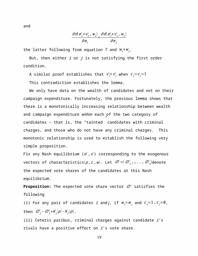
the latter following from equation 7 and w i>w j.

But, then either i or j is not satisfying the first order condition.

A similar proof establishes that vi¿>v j

¿ when c i=c j=1

This contradiction establishes the lemma.

We only have data on the wealth of candidates and not on their campaign expenditure.

Fortunately, the previous lemma shows that there is a monotonically increasing relationship

between wealth and campaign expenditure within each of the two category of candidates – that

11

is, the “tainted” candidates with criminal charges, and those who do not have any criminal

charges. This monotonic relationship is used to establish the following very simple proposition.

Fix any Nash equilibrium (e¿ , v¿) corresponding to the exogenous vectors of characteristics

( p , c , w). Let ∅ ¿=(∅ 1¿ ,… .. ,∅ n

¿ )denote the expected vote shares of the candidates at this Nash

equilibrium.

Proposition: The expected vote share vector ∅ ¿ satisfies the following

(i) For any pair of candidates i and j, if w i=w j and c i=1 , c j=0, then ∅ j¿−∅i

¿>K j ( p )−K i( p).

(ii) Ceteris paribus, criminal charges against candidate i’s rivals have a positive effect on i’s vote

share.

(iii) For any two candidates i and j , if c i=c j and w i>w j, then ∅ i¿−∅ j

¿>[ K ( p )−K ( p)].

Proof : (i) Consider two candidates i and j such that c i=1and c j=0. Also, assume thatw i=w j

. We first show that

h j(e¿)>hi(e

¿)

To see this, we need to show that e j¿>ei

¿. Given the assumptions we have made, vi¿>0 since c i=1.

Supposee i¿≥ e j

¿. Then, given w i=w j ,

∂ d i(e i¿+v i

¿ ,wi)∂ e i

¿ >∂ d j(e j

¿ , w i)∂ e j

¿

But,

∂ hi(e¿)

∂ ei¿ ≤

∂ h j(e¿)

∂ e j¿

The latter two inequalities show that either i or j is not satisfying equation 9.

Hence, e j¿>ei

¿ and so h j(e¿)>hi(e

¿). Moreover, Si (1 , v i¿)>0, and so this too reduces i's

expected vote share. From equation 4, it follows that

∅ j¿−∅i

¿>K j ( p )−K i( p)

(ii) This follows straightaway from the specification of the model. If c j=1, then S j (1 , v j¿ )>0

and hence gij¿¿.

(iii) Suppose w i>w j and c i=c j , K i ( p )=K j ( p ). Then, we know from lemma 1 that

e i¿>e j

¿

12

Moreover, if c i=c j=1, then

vi¿>v j

¿

It follows straightaway from equation 4 that

∅ i¿−∅ j

¿>K i ( p )−K i( p)

This concludes the proof of the proposition.

We discuss briefly the implications of the proposition for our regression exercise. Consider part

(i) of the proposition. Essentially, this says that once we have controlled for wealth and policy

platforms, then expected vote share will be lower for a tainted candidate. We will attempt to

verify this in the regression exercise by checking whether the criminal dummy has a negative

coefficient9. The implication of part (ii) of the proposition is straightforward - the coefficient on

the variable representing rival candidates with criminal charges should be positive. Finally, part

(iii) requires that the coefficient on the wealth variable should be positive. Notice that the

proposition leaves open the possibility that wealth has a differential impact on vote shares of

tainted and non-tainted candidates.

3. Econometric Specification and Data

We derive our regression equation from the model in the previous section. We are interested

in explaining the vote share of each candidate i. Our model specifies that the vote share should

depend negatively upon the dummy for criminal charges. Since the stigma attached to a tainted

candidate is decreasing in the number of other tainted rivals, we also include the number of other

candidates with charges within the constituency interacted with criminal charge dummy as an

explanatory variable. The nature of the dependence of vote share on wealth is more nuanced. The

wealth of candidate i himself should have a positive impact, while the wealth of other candidates

should have a non-positive effect since vote shares add up to one. It therefore makes sense to use

the relative wealth of candidate i as an explanatory variable. Morever, the wealth effect could

differ across the two categories of candidates with criminal charges and those who do not. We

accommodate this possibility by including wealth of the candidate interacted with the dummy for

criminal charges as an explanatory variable. Finally, we include other candidate characteristics

such as the level of education of the candidate, dummy for the incumbent candidates seeking

9 In the theoretical model, the only determinants are ( p , c , e , v). In the regression exercise, we will have additional controls.

13

reelection to Lok Sabha, and a dummy for the candidates contesting as members of the state

incumbent party(ies) in the regression equation. In robustness tests we also include age and

gender of the candidates.

So, our benchmark regression equation is:

Yi=α + βc Criminal dummyi + βw Relative Wealthi+ βcwCriminal dummyi * Wealthi + γs

Number of Candidates with Chargesi *Criminal dummyi+ βn Incumbencyi + βns State

Incumbenti + βe Dummies for high Education Statusi + γ Constituency Fixed Effects + λ

Party Fixed Effects + εi (11)

The vote share that we want to explain takes value between 0 and 1 and is bounded between

these limits. We transform the variable by calculating the log odds ratio for vote share of each

candidate and estimate the model by ordinary least squares, with heteroskedasticity corrected

standard errors. The dependent variable Y i is thus calculated as log( Vote sharei

1−vote share i) . In all our

regressions we include constituency fixed effects and party fixed effects to control for omitted

variables, such as the varying policy platforms of the candidates belonging to different political

parties. In robustness tests, we include fixed effects varying over state-party combinations

instead of the other fixed effects.

Another constraint is that the vote shares of all candidates add up to one within each

constituency. Therefore in our benchmark regressions we estimate the regressions either by

dropping all the candidates of a large party10, or all the candidates belonging to a large coalition

such as the UPA or NDA, one at a time. Since the vote shares of these large parties and

coalitions are significant (see Table ), the adding-up constraint does not apply any longer.

We describe the data used in the paper and also discuss the broad patterns observed in the

data. Our empirical results are presented in the next section.

In 2003, the Supreme Court in India decreed that all candidates contesting an election for

the Lok Sabha, Rajya Sabha, or state assemblies in India had to file an affidavit with the Election

Commission of India containing information on their assets (and liabilities), criminal charges and

education. We derive the data on these variables directly from the affidavits of the candidates-

10 We report results by dropping the candidates of the INC, BJP or BSP.

14

these are available on the election commission’s website as well as from a website maintained by

the Association for Democratic Reforms (ADR), http://myneta.info.

The data on percent of votes obtained, age, and gender of the candidates are obtained

from the election commission’s website. Information on candidate incumbency has been

gathered using various sources including searching through reports in the newspapers or on

various internet sites. We define a party as an incumbent in a state if it was in power in the state

(or was a major coalition partner), from 2008 up to the elections in 2009. The state level

incumbency information has been put together using the information contained in various articles

in the Economic and Political Weekly and elsewhere (see Appendix A1 and A2 for details). The

state level data on crime has been obtained from the National Crime Bureau Reports. Appendix

A1 provides the data sources from where the data on various variables have been obtained, while

Appendix A2 provides the summary statistics of the variables.

India has 28 states and 7 Union Territories (UTs) in all. Among the UTs, only Delhi has

its proper local administration with its own Chief Minister, while the remaining UTs are

administered by the center. Therefore, we include Delhi as a “state” in our sample while

excluding the remaining six UTs from the analysis. We follow Gupta and Panagariya (2012) and

exclude the eight northeastern states since they have a special status with deep involvement of

the center in their development process, as well as the state of Jammu and Kashmir. This leaves

us with a total of 20 states including Delhi. These states account for 506 out of the total of 543

parliamentary seats across the country.

Using the data from the affidavits, we define three categories for the education status of

the candidates, education up to high school, an undergraduate, and a post graduate or a technical

degree, and define different dummies for each one of them. Relative wealth is calculated as the

ratio of the wealth of the candidate to the average wealth of the rest of the candidates. In the

regressions, when we exclude all Independent candidates we calculate relative wealth as the ratio

of the candidate’s wealth to the average wealth of the other non-Independent candidates in the

constituency.

Each candidate’s affidavit has to contain information on whether the candidate faced

any criminal charges, as well as the sections of the Indian Penal Code (IPC) under which the

15

charges if any have been framed. In addition, the candidate has to declare whether he or she has

ever been convicted. Thus, in principle, the data is available on the number of criminal cases that

a candidate faces, the specific sections of the IPC under which the candidate faces these charges

and whether the candidate has ever been convicted. The ADR further divides the charges into

the charges for serious and non serious offences, by examining the sections of the IPC under

which the candidates face the charges. The conviction rate of candidates facing charges is very

low—out of the 1,155 candidates in the 2009 Lok Sabha elections who faced at least one

criminal charge, only 15 candidates were convicted.

It is sometimes claimed that the data on criminal charges is misleading since the charges

are sometimes initiated by political rivals. Moreover, some of the charges are associated with

involvement in political activities. In order to clean the data of such “spurious” charges, we

specify a value of one to the criminal dummy only when a candidate faces more than one charge.

This adjustment takes care of some obvious cases of frivolous charges or charges arising out of

political activities.11 Henceforth, we will use the term tainted candidate to denote a candidate

who has two or more criminal charges against them.

Consider now the patterns of criminal charges across candidates, states, and parties, and

at their correlates with other candidate specific factors for the 20 states that are included in our

regression analysis. Table 1 shows that it is the national and recognized state parties which field

a substantially higher proportion of tainted candidates. In fact, roughly one in seven candidates

fielded by state parties have at least two criminal charges levied against them. The

corresponding number for national parties is over one in ten candidates. This, together with the

fact that a substantially higher number of winning candidates come from the national and state

parties, explains why the win-ratio (the ratio of the number of successful candidates to the

number of contesting candidates) is substantially higher for tainted candidates. This is

documented in Table 2.

Table 3 shows the distribution of constituencies by the number of candidates who faced

at least two charges. On average, about 15 candidates contested the election in each constituency

in the 2009 Lok Sabha elections. Despite the large number of candidates, an overwhelming 11 As robustness checks, we choose alternative specifications where (i) the criminal dummy takes value one if a candidate has three or more criminal charges; or (ii) the number of criminal charges instead of a criminal dummy is used as an explanatory variable.

16

number of constituencies - over 75 per cent – had no tainted candidates. In other words, there

was a concentration of tainted candidates in some constituencies. In fact, states like Bihar,

Jharkand, Kerala had a concentration of tainted candidates.

Table 4 shows that on average, tainted candidates were wealthier, more likely to be

incumbents and obtained a much larger percent of the votes. Somewhat surprisingly, the average

age and education level of tainted candidates is also higher. Indeed, the difference in averages of

these variables are statistically significant at the 1 percent level.

4. Regression Results

We have pointed out in the last section that tainted candidates have a higher win ratio. At

first sight, this might suggest that voters do not care at all about the criminal records of their

elected representatives. This is misleading because of several reasons – tainted candidates are

more likely to be nominated by established political parties, and they have higher wealth. These

are obvious factors which influence vote shares and hence the win ratio. So, a more detailed

analysis is required because any conclusions can be drawn about the response of voters to tainted

candidates. This provides a strong motivation for our regression exercise.

We have two parallel sets of basic regressions. In the first, we estimate our regressions

using the data for all candidates in the twenty states that we have included in our analysis. We

then run the same regression on a smaller sample which includes only the candidates affiliated

with some political party, thus dropping the observations for “Independent” candidates. We drop

the Independent candidates since the majority of these candidates obtained only negligible vote

shares.12 Almost all the results are invariant with respect to the two samples.

Table 5 reports the basic regression results. Column I contains the results for our

benchmark specification. In subsequent columns we drop the candidates affiliated with the INC,

BJP, BSP, UPA and NDA respectively from the sample, in order to avoid the adding up

constraint. In Table 6 we carry out a similar exercise but after dropping the Independent

candidates from the data.

12 There were 3825 independent candidates with an average vote share of about 0.80 percent. Only 10 Independent candidates won in the 2009 election.

17

The variables we are particularly interested in are the criminal dummy variable, relative

wealth, as well as the interaction of the criminal dummy with wealth and with the number of

other candidates with criminal charges in the constituency. Table 5 shows that our results are

remarkably consistent with the theoretical model of Section 2. Importantly, the qualitative

results hold irrespective of which party or coalition is dropped from the sample in order to take

care of the adding-up constraint. Thus, the negative coefficient on the criminal dummy shows

that tainted candidates lose vote share relative to the others. Relative wealth has a positive effect

on vote shares. The coefficient of relative wealth interacted with the criminal charge dummy is

positive, implying that the loss in vote share is smaller for a wealthier candidate. Similarly, the

coefficient of the interaction between the number of other tainted candidates with criminal

charges and the criminal dummy is positive and significant in the regressions for all the

candidates. This implies that the stigma attached to being a tainted candidate declines if there are

other tainted candidates in the constituency.

Among other results, the high education status of the candidates has a positive effect on

vote share. We also find that incumbency at the candidate level as well as at the party level in the

state increases the vote share of the candidates.13 Most of these results are robust to the exclusion

of Independent candidates from the sample.

We now report on some robustness checks. Since the primary purpose of the paper is to

throw light on voter response to tainted candidates, we conduct a key robustness test by

constructing the dummy for criminal charges in an alternative way. This dummy takes value 1 if

the candidate faces at least three criminal charges (instead of two in the earlier specification), and

zero otherwise. Construction of the dummy in this way reduces the possibility of labeling a

candidate as tainted if the charges against him are politically motivated or perhaps arising from

violations of the law while undertaking political activities. The results are qualitatively similar to

the ones obtained earlier for most of the variables. The coefficients of the criminal dummy and

the interaction between wealth and criminal dummy are somewhat larger than before, thus

indicating that the loss of vote share is larger for a candidate who faces three or more charges

13 Gupta and Panagariya (2011) also come to the same conclusion. Of course, the positive effect of incumbency may be due to the fact that the coalition of parties constituting the UPA retained power in 2009. There are other instances where the ruling party or coalition has been defeated in the election- in such cases, we would not expect to observe a positive effect of incumbency on vote shares.

18

than for the candidates with at least two charges. For such candidates, additional wealth helps in

reducing the stigma by a larger amount as well.

Table 7 reports some additional robustness checks. Column III in Table 7 includes the

interaction of state incumbent and criminal dummy, while column IV includes age and gender of

the candidate in the regressions. Finally, in the last column we include the number of all

candidates with criminal charges in a constituency rather than only against the top four

candidates by vote share, interacted with the dummy for criminal candidates.

The results show that the coefficients of the main variables of interest—wealth or

relative wealth, criminal dummy and the interaction of wealth and criminal dummy, retain their

significance. The only variable which loses significance in some of the specifications is the

interaction of the number of charges against other candidates with criminal dummy.

Some other robustness tests are reported in Table 8. In column I, relative wealth is

calculated as the ratio of the candidate’s own wealth to the sum of the wealth of candidates who

received at least 3 percent of the total votes. Similarly, the number of candidates with charges

also includes the data for only these candidates. In column II we estimate the regressions using

the data only for the constituencies reserved for candidates from the scheduled castes and

schedule tribes. In the last column we estimate the regressions only for the constituencies which

are not reserved for the candidates of the schedules or scheduled tribes. Again all our main

results hold— the criminal dummy has a negative coefficient, wealth or relative wealth has a

positive coefficient, and the interaction of wealth and criminal dummy has a positive coefficient.

The coefficient of other candidates with charges is mostly positive, but insignificant in some of

the specifications.

We have conducted two more robustness tests, but do not report the results. In one, we

drop one state at a time and estimate our benchmark specification with the rest of the data. All of

our results hold with minor variations in the coefficients or the significance levels. This

robustness test confirms that our results are not driven by any outlier state. Second we estimate

regressions similar to those in Table 7 by eliminating the Independent candidates from the

sample. The qualitative results remain unchanged.

19

These results seem to leave very little doubt that voters do punish tainted candidates –

this conclusion remains true irrespective of the specification chosen by us, and also remains true

when we leave Independents out of the regression exercise. However, this raises the obvious

question. Why do political parties nominate so many tainted candidates when they have so many

other aspiring candidates fighting for a party ticket? As we have mentioned earlier, Aidt et al

(2010) construct a theoretical model which assumes that tainted candidates have some electoral

advantage which induces political parties to nominate them despite some reputational cost. They

do not specify the nature of the electoral advantage, but mention in passing that it could be the

power of criminal candidates to intimidate voters who are likely to vote for their rivals. If this

were the case, then one would expect voter turnout to be lower the greater is the number of

tainted candidates. Table 9 negates this hypothesis – the data seem to show no negative

relationship between voter turnout and the number of tainted candidates in a constituency.

An alternative hypothesis advanced by Vaishnav (2010) is that tainted candidates are

wealthier. In fact, he finds empirical support for this hypothesis in his data set which consists of

elections in various state assemblies. As Table 10 shows, this seems to be true even in our

sample. So, it seems plausible to argue that tainted candidates use their greater wealth to “buy”

their tickets. They can use their wealth to campaign more intensively, and perhaps also

contribute to party funds. Unfortunately, we have no data (other than the self-reported wealth of

the candidates) to empirically verify any other hypothesis.

5. Conclusion

Our main empirical results suggest that voters do punish candidates who have criminal

charges against them. However, these tainted candidates are able to overcome this electoral

disadvantage because they have greater wealth, and wealth plays a significant role in increasing

vote shares. The most plausible channel through which wealth affects vote shares is of course

through campaign expenditures, which are likely to be positively related to wealth.

There is now a fair body of evidence suggesting that voters who have information about

the corrupt ion of incumbent politicians do punish the latter. For instance, Ferraz and Finan

(2008) use detailed Brazilian electoral and audit data to show that new information about

20

political corruption reduces the probability of reelection for corrupt incumbents. Bobonis et al

(2011) find that publicly available pre-election municipal audits significantly reduce the level of

corruption in Puerto Rican municipalities.14 Closer home, Banerjee et al (2011) conclude, on

the basis of a field experiment conducted before the Delhi state legislative elections , that

voters who had access to information about incumbent performance punished worse

performing incumbents and those facing better quailed challengers – these incumbents then

received significantly fewer votes.

Our empirical results, along with this body of evidence suggests that it is important for

voters to be better informed about candidate characteristics. The mere requirement that

candidates file affidavits with the Election Commission about their characteristics is of limited

use if voters do not have access to this information. Perhaps, the Election Commission needs to

play a more active role in disseminating this information. The Commission must also think

seriously about enhancing the existing ceilings on campaign expenditure since practically no

candidate or party adheres to the current limits on expenditure. However, the Commission must

ensure that all candidates adhere to the enhanced (but realistic) ceiling. This will then at least

reduce the “wealth advantage” enjoyed by tainted politicians.

14 See also Brollo(2011),

21

References

Aidt, Toke, Miriam Golden and Devesh Tiwari, 2011, “Incumbents and Criminals in the IndianNational Legislature.” , Department of Political Science, University of California-Los Angeles.

Banerjee, Abhijit V. and Rohini Pande, 2009, “Parochial Politics: Ethnic Preferences and Political Corruption.”

Banerjee, Abhijit V. and Rohini Pande, Selvan Kumar and Felix Su, 2011, “Do informed voters make better choices? Experimental Evidence from Urban India.”

Bobonis Gustavo J., Luis R. Cámara Fuertes, and Rainer Schwabe, 2009, “Does Exposing Corrupt Politicians Reduce Corruption?”.

Brollo, Fernanda, 2011, “Why do Voters Punish Corrupt Politicians? Evidence from the Brazilian Anti-Corruption Program”.

Chemin, Matthieu, 2008, “Do Criminal Politicians Reduce Corruption? Evidence from India.” Working Paper 08-25, Department of Economics, University of Quebec at Montreal.

Ferraz, C. and F. Finan (2008), “Exposing Corrupt Politicians: The Effects of Brazil’s Publicly Released Audits on Electoral Outcomes”, Quarterly Journal of Economics 123 (2), 703–745.

Gupta, Poonam and Arvind Panagariya, 2012, Growth and Election Outcomes in a Developing Country.

Paul, Samuel and M. Vivekananda, 2004, “Holding a Mirror to the New Lok Sabha.”Economic and Political Weekly (November 6).

Vaishnav, Milan, 2010, “The Market for Criminality: Money, Muscle and Elections in India.” Typescript, Columbia University.

22

Appendix A1: Description and Data Sources of Variables

Variable Source Description

Dependent Variable Election Commission and own calculation

The dependent variable for candidate i is calculated as

log( Vote sharei

1−vote share i)

Criminal Dummy Election Commission and Association for Democratic Reforms (ADR)

The dummy takes a value 1 if the candidate has two or more criminal cases against him, and zero otherwise. In robustness tests the dummy takes a value 1 if the candidate has three or more cases against him.

Wealth*Criminal Dummy

Election Commission Interaction variable calculated as Log wealth x dummy for criminal charges

Relative wealth Election Commission and own calculation

Wealth of the candidate/average wealth of all other candidates in the constituency

Candidates with charges Election Commission and ADR

Number of candidates within the constituency who face criminal cases. In most specifications, as mentioned in the tables, we look at the number of such candidates within top four candidates by vote share, and in robustness tests we include the number of all candidates with charges within the constituency.

Candidates with charges*criminal dummy

Election Commission and ADR and own construction

Interaction between number of candidates with charges and criminal charges dummy.

Education: Dummy for Undergraduate Degree

Dummy for Masters Degree

Election Commission Dummy for Undergraduate Degree takes a value 1 if a candidate has education up to undergraduate, and zero otherwise; and Dummy for Masters Degree takes a value 1 for education level higher than undergraduate (or for a technical or professional degree) and zero otherwise.

Age Election Commission In yearsGender dummy Election Commission Dummy takes a value 1 if the candidate is a female, and 0

otherwiseIncumbent Member of Parliament

Various sources on the web

The dummy takes a value 1 if the candidate was a member of the previous Lok Sabha, and zero otherwise.

State Incumbent party Various sources on the web and different issues of Economic and Political Weekly

The dummy takes a value 1 if the candidate belongs to a party which was in power in state government in 2008-09 before the Lok Sabha Elections. The state incumbent parties are: Andhra Pradesh, Indian National Congress (INC), TRS; Bihar: JDU, Bhartiya Janata Party (BJP); Chhattisgarh: BJP; Delhi: INC; Goa: INC, NCP; Gujarat: BJP; Himachal Pradesh: BJP; Haryana: INC; Kerala: CPI ( Marxist), CPI; Maharashtra: INC, NCP; Madhya Pradesh: BJP; Orissa: Biju Janata Dal; Punjab: Siromani Akali Dal, BJP; Rajasthan: BJP; Tamil Nadu: Dravida Munnetra Kazhagam, INC; Uttarakhand: BJP; Uttar Pradesh: Bajuhan Samaj Party; West Bengal: CPI (Marxist), RSP; Karnataka: BJP; Jharkhand: JMM, BJP

23

Appendix A2: Summary Statistics of Variables

Variable Observations Average Minimum MaximumPercent of Votes Obtained 7192 6.82 0.02 78.80

log( Vote sharei

1−vote share i) 7192 -4.61 -8.52 1.31

Criminal dummy (at least two cases) 7173 0.07 0 1Number of candidates with charges (in top four candidates) 7192 1.22 0 4Relative wealth 7192 2.26 0.00 452.22Wealth (1000s) log 7192 13.81 0.69 22.57Education dummy for undergrad degree 6749 0.22 0 1Education dummy for masters degree 6749 0.27 0 1Incumbent Member of Parliament 7192 0.05 0 1State incumbency party 7192 0.07 0 1Age 7191 45.98 25 88Gender Dummy 7192 0.07 0 1*we drop three outliers from the regressions when the relative wealth exceeded 500. Statistics ate given for the data for twenty states that we have used in the paper.

24

Table 1: Candidates with Criminal Cases across Party Types

Party Type Number of Candidates

Number of Candidates with least 2 Criminal Cases

% of CandidatesWith at least 2 Criminal Cases

I II III: (II/1)*100National Parties 1353 176 11.5State Parties 585 108 15.6Unrecognized Parties 1790 110 6.2Independent Candidates 3659 124 3.4

Source: Authors’ own calculations using the data mentioned in Appendix A1; data refer to the observations on twenty states included in the regressions.

Table 2: Distribution of Contesting and Winning Candidates by the number of Criminal Cases

Number of Criminal

Cases

Number of Candidates

Number of Winning

CandidatesI II III0 6,551 349

1 607 73

2-4 382 57

5-9 92 16

>10 44 10

Total 7676 506

Source: Authors’ own calculations using the data mentioned in Appendix A1; data refer to the observations on twenty states included in the regressions.

25

Table 3: Distribution of Candidates with Charges across Constituencies

Number of candidates with at least two charges

Number of constituencies

0 2061 1692 833 254 145 9

Source: Authors’ own calculations using the data mentioned in Appendix A1, data refers to the observations on twenty states included in the regressions.

Table 4: A Comparison of Variables for Candidates with and without Criminal Charges(at least two Criminal Charges)

Criminal Dummy

% votes Age Log Assets(in 1000s)

Education Index

Incumbent(percent)

0 5.9 45.7 13.7 2.57 4

1 15.4*** 47.2*** 15.1*** 2.71*** 10***

Total 6.59 45.8 13.81 2.58 5

Source: Authors’ own calculations using the data mentioned in Appendix A1; data refer to the observations on twenty states included in the regressions. *** indicates that the values are significantly different from those for candidates with one or no charges at 1 percent level of significance.

26

Table 5: Explaining the Vote Share of Candidates—Benchmark Specification (All Candidates)

I II III IV V VIAll Drop

INCDrop BJP

Drop BSP

Drop UPA

Drop NDA

Criminal Dummy -1.06*** -1.05*** -1.04*** -1.27*** -1.05*** -0.88**(2.83) (2.83) (2.70) (3.30) (2.74) (2.30)

Candidates with Charges (among top 4) 0.25*** 0.25*** 0.29*** 0.26*** 0.24*** 0.29****criminal dummy (4.48) (4.37) (4.71) (4.38) (4.03) (5.10)Relative Wealth 0.007*** 0.012**

*0.007*** 0.007*** 0.013*** 0.007***

(3.02) (4.51) (2.81) (2.65) (4.11) (2.90)Wealth log*Criminal Dummy 0.082*** 0.084**

*0.081*** 0.096*** 0.084*** 0.066**

(3.19) (3.27) (3.01) (3.64) (3.16) (2.46)Education dummy for undergrad degree 0.14*** 0.13*** 0.13*** 0.16*** 0.12*** 0.119***

(4.03) (3.63) (3.55) (4.33) (3.35) (3.23)Education dummy for masters degree 0.26*** 0.25*** 0.257*** 0.25*** 0.24*** 0.244***

(7.16) (6.79) (6.95) (6.74) (6.42) (6.61)State Incumbent 1.76*** 2.054**

*1.910*** 1.599*** 1.961*** 1.798***

(24.10) (24.18) (19.89) (18.75) (21.89) (18.28)Incumbent Member of Parliament 1.77*** 2.06*** 1.91*** 1.60*** 1.97*** 1.80***

(24.15) (24.29) (19.99) (18.69) (21.99) (18.38)Fixed Effects for Constituencies Yes Yes Yes Yes Yes YesFixed Effects for Parties Yes Yes Yes Yes Yes YesObservations 6,729 6,338 6,341 6,281 6,145 6,213Adj. R-squared 0.78 0.76 0.764 0.79 0.75 0.76*,**, *** indicate that the coefficient is significantly different from zero at 10, 5 and 1 percent levels of significance respectively. Robust t statistics are reported in parentheses. The regression equation is in equation 8 and the variables are defined in Appendix A1 and in the text. The dependent variable is

calculated as log( Vote sharei

1−vote share i) . In column I we estimate the regression for all the candidates.

In column II -VI we drop candidates belonging to specific parties or coalition groups form the sample of non independent candidates. so in column II we drop the candidates belonging to the Indian national congress from the sample, in Column III we drop all candidates belonging to BJP, in Column IV we drop the candidates of BSP, in Column V we drop candidates who belong to any of the parties who were a part of the coalition of parties which contested the election as a part of the United progressive alliance, and in column VI we drop all parties which contested the election as a part of the national democratic alliance.

27

Table 6: Explaining the Vote Share of Candidates (Candidates who are affiliated with a Political Party)

I II III IV V VIParty

affiliated

Drop INC

Drop BJP

Drop BSP

Drop UPA

Drop NDA

Criminal Dummy -0.97* -1.04** -0.85* -1.20** -1.18** -0.59(1.93) (2.17) (1.65) (2.21) (2.21) (1.15)

Candidates with charges (among top 4)

0.198***

0.17** 0.23*** 0.21** 0.160* 0.26***

*criminal dummy (2.60) (2.18) (2.76) (2.48) (1.88) (3.06)Relative Wealth 0.009* 0.009** 0.012**

*0.009* 0.009**

(1.79) (2.41) (3.52) (1.65) (2.48)Wealth log*Criminal Dummy 0.079** 0.089**

*0.07** 0.095**

*0.096**

*0.05

(2.37) (2.79) (2.13) (2.64) (2.71) (1.48)Education dummy for undergrad degree

0.23*** 0.19*** 0.18*** 0.25*** 0.16** 0.15**

(2.76) (2.94) (2.70) (3.83) (2.49) (2.30)Education dummy for masters degree 0.35*** 0.32*** 0.36*** 0.36*** 0.29*** 0.33***

(4.37) (5.33) (5.70) (5.70) (4.69) (5.25)State Incumbent 1.74*** 2.0*** 1.87*** 1.64*** 1.91*** 1.76***

(23.95) (23.05) (17.95) (18.53) (20.44) (16.60)Incumbent Member of Parliament 0.78*** 0.99*** 0.89*** 0.86*** 1.02*** 0.89***

(8.88) (9.21) (8.08) (9.29) (8.87) (7.80)Fixed Effects for Constituencies Yes Yes Yes Yes Yes YesFixed Effects for Parties Yes Yes Yes Yes Yes YesObservations 3,629 3,227 3,231 3,172 3,037 3,103Adj. R-squared 0.774 0.766 0.76 0.787 0.768 0.763*,**, *** indicate that the coefficient is significantly different from zero at 10, 5 and 1 percent levels of significance respectively. Robust t statistics are reported in parentheses. The regression equation is in equation 11 and the variables are defined in Appendix A1 and in the text. The dependent variable is

calculated as log( Vote sharei

1−vote share i) . In column I we estimate the regression for the candidates who

are affiliated with a political party, so we drop all independent candidates from the sample. In column II -VI we drop candidates belonging to specific parties or coalition groups from the sample of non independent candidates. so in column II we drop the candidates belonging to the Indian national congress from the sample, in Column III we drop all candidates belonging to

28

BJP, in Column IV we drop the candidates affiliated with BSP, in Column V we drop candidates who belong to any of the parties who were a part of the coalition of parties which contested the election as a part of the United progressive alliance, and in column VI we drop candidates of all parties which contested the election as a part of the national democratic alliance.

29

Table 7: Explaining the Vote Share of Candidates: Robustness TestsI II III IV V

Criminal Dummy -1.27*** -0.98*** -1.02**(3.30) (2.65) (2.53)

Criminal Dummy (more than 2 cases) -1.15* -1.45**(1.87) (2.15)

Candidates with charges (among top 4)* 0.28*** 0.195**criminal dummy (>2cases) (3.76) (2.03)Candidates with charges (among top 4) 0.27*** 0.25****criminal dummy (4.84) (4.43)Candidates with charges*criminal dummy 0.037

(1.22)Relative Wealth 0.008*** 0.007*** 0.007*** 0.007***

(3.22) (2.88) (3.00) (2.98)Relative Wealth (no independents) 0.008***

(2.69)Wealth log*criminal dummy 0.099*** 0.078*** 0.10***

(3.71) (3.03) (3.95)Wealth log*criminal dummy (>2 cases) 0.089** 0.113***

(2.21) (2.63)Education dummy for undergrad degree 0.15*** 0.22*** 0.14*** 0.14*** 0.14***

(4.17) (3.60) (4.02) (4.04) (4.01)Education dummy for masters degree 0.26*** 0.35*** 0.25*** 0.25*** 0.25***

(7.25) (6.09) (7.10) (6.92) (7.10)State Incumbent 1.79*** 1.76*** 1.85*** 1.77*** 1.78***

(24.37) (24.12) (24.06) (24.18) (24.31)Incumbent Member of Parliament 0.84*** 0.78*** 0.83*** 0.82*** 0.84***

(9.59) (8.82) (9.57) (9.43) (9.56)State Incumbent*Criminal Dummy -0.52***

(3.26)Age 0.005***

(3.78)Gender 0.036

(0.69)Fixed Effects for Constituencies Yes Yes Yes Yes YesFixed Effects for Parties Yes Yes Yes Yes YesObservations 6,729 3,618 6,729 6,728 6,729Adj. R-squared 0.781 0.772 0.783 0.783 0.781

*,**, *** indicate that the coefficient is significantly different from zero at 10, 5 and 1 percent levels of significance respectively. Robust t statistics are reported in parentheses. The regression equation is in equation 11 and the variables are defined in Appendix A1 and in the text. The dependent variable is

30

calculated as log( Vote sharei

1−vote share i) . In column I and II we include a new criminal charge dummy,

which takes a value 1 only if the candidates face at least three charges. In column I we estimate the regression for all the candidates and in column II we estimate the regression after dropping independent candidates from the regression. In Column III we include the interaction of state incumbent and criminal dummy. In column IV we include age and gender of the candidates in the regressions, and in Column V, we include the interaction variable of all candidates with charges in the constituency and criminal dummy (rather than the candidates with charges among top four candidates interacted with criminal dummy).

31

Table 8: Explaining the Vote Share of Candidates: More Robustness Tests

I II IIIDifferent Reference group for relative wealth

Only Reserved Constituencies

Only General Constituencies

Criminal Dummy -1.08*** -1.79* -0.85**(2.86) (1.87) (2.01)

Candidates with charges (at least 3 pc vote share) 0.08*criminal dummy (1.42)Candidates with charges (among top 4) 0.30* 0.25****criminal dummy (1.91) (4.00)Relative Wealth (candidates with at least 3 pc votes)

0.013***

(4.10)Relative Wealth 0 0.009***

(0.15) (4.56)Wealth log*criminal dummy 0.109*** 0.140** 0.064**

(4.49) (1.97) (2.26)Education dummy for undergrad degree 0.14*** 0.19** 0.11**

(3.98) (2.53) (2.54)Education dummy for masters degree 0.26*** 0.39*** 0.21***

(7.14) (4.83) (4.95)State Incumbent 1.79*** 1.71*** 1.76***

(24.52) (11.30) (20.41)Incumbent Member of Parliament 0.82*** 0.66*** 0.88***

(9.37) (3.24) (8.62)Fixed Effects for Constituencies Yes Yes YesFixed Effects for Parties Yes Yes YesObservations 6,715 2,021 4,708Adj. R-squared 0.781 0.764 0.787

*,**, *** indicate that the coefficient is significantly different from zero at 10, 5 and 1 percent levels of significance respectively. Robust t statistics are reported in parentheses. The regression equation is in equation 11 and the variables are defined in Appendix A1 and in the text. The

dependent variable is calculated as log( Vote sharei

1−vote share i) . In column I, relative wealth is

calculated with respect to the wealth of the candidates who obtained at least 3 percent of the vote share. In column II we estimate the regression for only the candidates who contested elections from a constituency reserved for the candidates of scheduled castes or scheduled tribes; in Column III we estimate the regression for the unreserved constituencies.

32

Table 9: Voter Turnout and the Number of Candidates with Criminal Charges(Dependent Variable: Percent of Eligible Voters who voted)

I II III IV V VINumber of Candidates with at least two Charges

0.079 0.34 0.23 0.20

(0.28) (1.21) (0.79) (0.72)Total Candidates -0.23*** -0.24*** -0.23***

(4.14) (4.30) (4.18)Number of Candidates with at least 0.861** 1.0**Two Charges from a Large Party (2.08) (2.38)Total Candidates from a Large Party -0.579*

(1.86)Dummy for a Constituency Reserved -2.25*** -1.25 -1.397* -2.23***for the Scheduled Caste Candidates (2.91) (1.65) (1.83) (2.85)Dummy for a Constituency Reserved 1.14 2.61** 2.74** 0.51for the Scheduled Tribe Candidates (0.94) (2.24) (2.31) (0.41)Literacy -0.093**

(2.09)State Fixed Effects Yes Yes Yes Yes Yes YesObservations 506 506 506 506 506 506Adj. R-squared 0.78 0.788 0.792 0.784 0.785 0.794

*,**, *** indicate that the coefficient is significantly different from zero at 10, 5 and 1 percent levels of significance respectively. Robust t statistics are reported in parentheses. Dependent variable is percent of eligible voters who voted. Regressions are estimated using linear regressions. A large party refers to a national or a state party. Literacy rate refers to the rate of literacy for each constituency in 2008, the data for which is obtained from Indicus Analytics.

33

Table 10: Candidate Wealth and Criminal Dummy(Dependent Variable: Candidate wealth)

I II III IV VCriminal Dummy 0.779**

*0.781*** 0.646*** 0.762*** 0.714***

(7.57) (7.58) (6.27) (5.79) (6.06)Dummy for National Party 2.577**

*2.072*** 1.924***

(42.74) (31.15) (22.36)Dummy for State Party 1.882**

*1.625*** 1.426***

(19.82) (17.55) (13.21)Education dummy for undergrad degree

0.744*** 0.648*** 0.656*** 0.701***

(11.11) (9.79) (5.29) (7.37)Education dummy for masters degree 1.041*** 0.820*** 1.020*** 1.021***

(16.07) (12.51) (8.63) (11.88)Incumbent Member of Parliament 1.135*** 0.872*** 1.097*** 1.041***

(11.64) (8.41) (10.54) (10.71)Fixed Effects for Constituencies Yes Yes Yes Yes YesFixed Effects for Parties No No Yes No NoObservations 7,173 6,733 6,729 2,075 3,629Adj. R-squared 0.253 0.305 0.372 0.208 0.29*,**, *** indicate that the coefficient is significantly different from zero at 10, 5 and 1 percent levels of significance respectively. Robust t statistics are reported in parentheses. Dependent variable is log wealth of the candidates. Dummy for national party takes a value 1 if the candidate belongs to a national party, and zero otherwise; dummy for a state party takes a value 1 if the candidate belongs to a state party, and zero otherwise. In column IV we estimate regressions only for the candidates of national parties; and in Column V regressions are estimated only for candidates who are affiliated with one of the political party, thus dropping the independent candidates.

34