· web viewlogistic regression shares the same objective as linear regression. logistic and linear...

Regression with a Dichotomous Dependent Variable:An Introduction to Logistic Regression

to accompany

Prepared by

Steven Prus

Carleton University

Copyright © 2013 by Nelson Education Ltd.

Regression with a Dichotomous Dependent Variable: An Introduction to Logistic Regression to accompanyStatistics: A Tool for Social Research, Second Canadian EditionBy Joseph F. Healey and Steven G. Prus

COPYRIGHT © 2013 by Nelson Education Ltd. Nelson is a registered trademark used herein under licence. All rights reserved.

For more information, contact Nelson, 1120 Birchmount Road, Toronto, ON M1K 5G4. Or you can visit our Internet site at www.nelson.com.

ALL RIGHTS RESERVED. No part of this work covered by the copyright hereon may be reproduced or used in any form or by any means—graphic, electronic, or mechanical, including photocopying, recording, taping, web distribution or information storage and retrieval systems—without the written permission of the publisher.

Copyright © 2013 by Nelson Education Ltd.

Regression with a Dichotomous Dependent Variable: An Introduction to Logistic RegressionIntroductionIn the on-line chapter titled “Linear Regression with Dummy Variables,” we looked at how to use a dichotomous (dummy) independent variable in linear regression. It is also possible that the dependent variable be a dichotomous variable. In this situation we commonly use a statistical technique similar to linear regression called logistic regression.

Logistic regression shares the same objective as linear regression. Logistic and linear regression are statistical methods used to predict the dependent variable based on one or more independent variables. They both produce a regression model to summarize the relationship between these variables, as well as other statistics to describe how well the model fits the data. Accordingly, you may wish to review the material on linear regression in Chapters 13 and 14 before reading any further.

While linear and logistic regression are forms of regression analysis, the former is used for the modeling of an interval-ratio dependent variable and the latter for a dichotomous (dummy) variable. Both procedures require the independent variable to be measured at the interval-ratio level, though nominal and ordinal independent variables can be converted to a set of dummy variables. Here, we will consider the simplest (bivariate) form of logistic regression, though like linear regression, it can be extended to include more than one independent variable.

Probabilities, Odds, and Logits

To understand logistic regression, we must first understand the concepts of probabilities, odds, and logits. Each concept is considered in turn.

Probabilities In logistic regression, the dependent variable is a dichotomous variable, coded as 1 for the category of “interest” or “success” and 0 for the “reference” or “failure” category. Specifically, we are interested in the probability that the dependent variable, Y, equals 1. 1

As defined in Chapter 4 of your textbook, a probability, p, is the likelihood that a particular event will occur. The probability of an event, which ranges from 0 to 1, is expressed by the ratio of the number of actual occurrences of the event to the total number of possible occurrences of the event:

FORMULA 1 Probability ( p )= number of occurrences of eventnumber of possibleoccurrences of event

1 The category of interest/success is arbitrarily selected by the researcher, so the researcher chooses which category to code as 1.

1 Copyright © 2013 by Nelson Education Ltd.

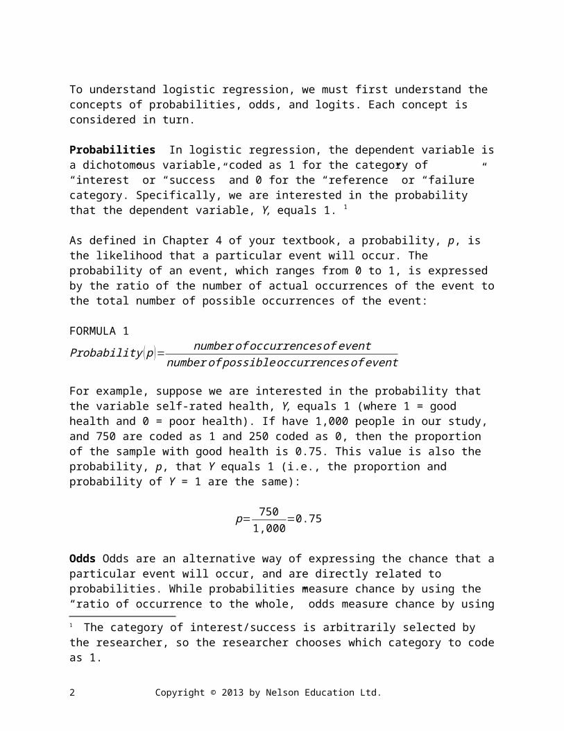
For example, suppose we are interested in the probability that the variable self-rated health, Y, equals 1 (where 1 = good health and 0 = poor health). If have 1,000 people in our study, and 750 are coded as 1 and 250 coded as 0, then the proportion of the sample with good health is 0.75. This value is also the probability, p, that Y equals 1 (i.e., the proportion and probability of Y = 1 are the same):

p= 7501,000

=0.75

Odds Odds are an alternative way of expressing the chance that a particular event will occur, and are directly related to probabilities. While probabilities measure chance by using the “ratio of occurrence to the whole,” odds measure chance by using the “ratio of occurrence to non-occurrence.” That is, odds are the ratio of the probability that an event will occur to the probability that it will not occur:

FORMULA 2 odds= p1−p

where p = probability of Y = 1.

Continuing with our previous example, if the probability of good health (Y = 1) is 0.75, then the odds of good health occurring are:

odds= 0.75(1−0.75 )

=0.750.25

=3

So, the odds of good health are 3 to 1, often written as 3:1.

As another example, if the probability of rain tomorrow (Y = 1) is 0.80 (i.e., if there’s an 80% chance of rain tomorrow), then the odds of rain occurring tomorrow are 4 to 1:

odds= 0.80(1−0.80 )

=0.800.20

=4

Odds Ratio Extending our discussion of odds, we call the ratio of two odds an “odds ratio,” symbolized as OR. That is, the odds ratio is the ratio of the odds of an event occurring (odds that Y =1) in one group to the odds of the event occurring (odds that Y =1) in another group. The groups might be men and women, lower educated persons and higher educated persons, and so on. We write the formula for the odds ratio as:

FORMULA 3 odds ratio(¿)=( p1

1−p1)

( p2

1−p2 )=

odds1

odds2


where p1 = probability of Y = 1 in Group 1p2 = probability of Y = 1 in Group 2

For example, let's say that 90% of persons with a post-secondary education (Group 1) and 75% of persons with a high-school education or less (Group 2) have good health. Thus, the odds of good health for persons with a post-secondary education are 0.90/0.10 = 9 and the odds of good health for persons with a high-school education or less are 0.75/0.25 = 3. Hence, the odds ratio is 9/3 = 3; that is, the odds of person with a post-secondary education having good health are 3 times higher than the odds of a person with a high-school education or less:

odds ratio(¿)=( 0.9

1−0.90 )( 0.75

1−0.75 )=9

3=3

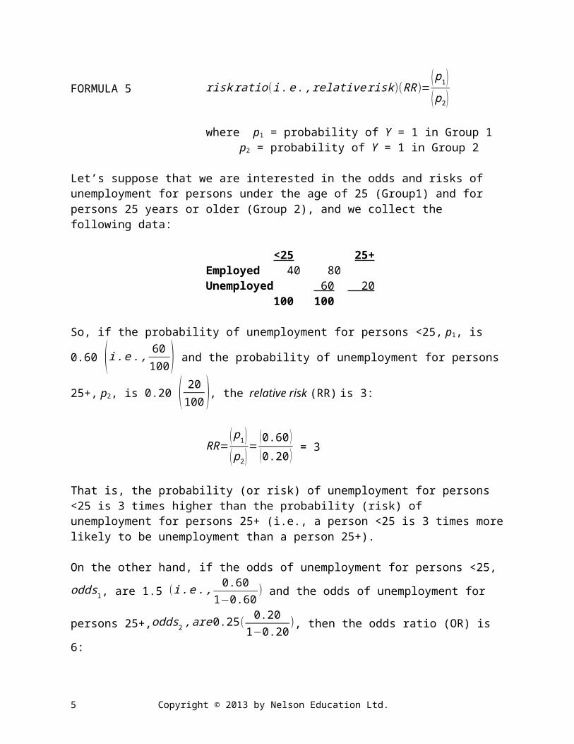
Odds Ratio vs. Relative Risk As a caveat to this discussion, it is sometimes the case that people mistake the odds ratio (OR) for the risk ratio, sometimes called the relative risk, (RR), though they are different statistical concepts.

The risk ratio is the ratio of the probability of the event occurring in one group relative to another group while the odds ratio is a ratio of the odds of the event occurring in one group relative to another group. Hence, the RR is the ratio of probabilities and the OR the ratio of odds:

FORMULA 4 odds ratio(¿)=( p1

1−p1)

( p2

1−p2 )=

odds1

odds2

FORMULA 5 risk ratio(i . e . , relativerisk )(RR)=( p1 )( p2 )

where p1 = probability of Y = 1 in Group 1 p2 = probability of Y = 1 in Group 2

Let’s suppose that we are interested in the odds and risks of unemployment for persons under the age of 25 (Group1) and for persons 25 years or older (Group 2), and we collect the following data:

<25 25+Employed 40 80Unemployed 60 20

100 100


So, if the probability of unemployment for persons <25, p1, is 0.60 (i . e . , 60100 ) and the

probability of unemployment for persons 25+, p2, is 0.20 ( 20100 ), the relative risk (RR) is 3:

RR=( p1 )( p2 )

=(0.60 )(0.20 ) = 3

That is, the probability (or risk) of unemployment for persons <25 is 3 times higher than the probability (risk) of unemployment for persons 25+ (i.e., a person <25 is 3 times more likely to be unemployment than a person 25+).

On the other hand, if the odds of unemployment for persons <25,odds1, are 1.5 (i . e . , 0.601−0.60

)

and the odds of unemployment for persons 25+,odds2 ,are 0.25 ( 0.201−0.20

), then the odds ratio

(OR) is 6:

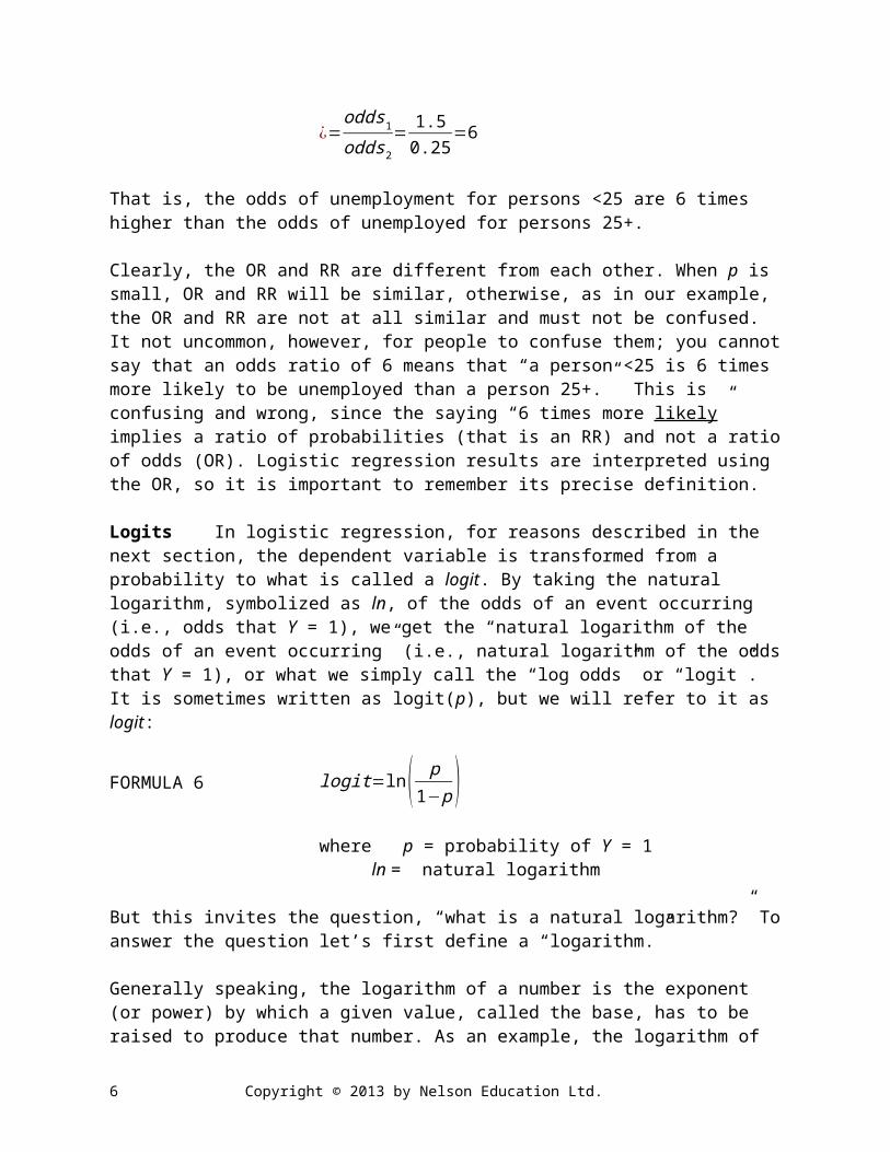
¿=odds1

odds2= 1.5

0.25=6

That is, the odds of unemployment for persons <25 are 6 times higher than the odds of unemployed for persons 25+.

Clearly, the OR and RR are different from each other. When p is small, OR and RR will be similar, otherwise, as in our example, the OR and RR are not at all similar and must not be confused. It not uncommon, however, for people to confuse them; you cannot say that an odds ratio of 6 means that “a person <25 is 6 times more likely to be unemployed than a person 25+.” This is confusing and wrong, since the saying “6 times more likely” implies a ratio of probabilities (that is an RR) and not a ratio of odds (OR). Logistic regression results are interpreted using the OR, so it is important to remember its precise definition.

Logits In logistic regression, for reasons described in the next section, the dependent variable is transformed from a probability to what is called a logit. By taking the natural logarithm, symbolized as ln, of the odds of an event occurring (i.e., odds that Y = 1), we get the “natural logarithm of the odds of an event occurring” (i.e., natural logarithm of the odds that Y = 1), or what we simply call the “log odds” or “logit”. It is sometimes written as logit(p), but we will refer to it as logit:

FORMULA 6 logit=ln( p1−p )

where p = probability of Y = 1ln = natural logarithm


But this invites the question, “what is a natural logarithm?” To answer the question let’s first define a “logarithm.”

Generally speaking, the logarithm of a number is the exponent (or power) by which a given value, called the base, has to be raised to produce that number. As an example, the logarithm of the number 100 to base 10 is 2 (i.e., 100 is 10 to the power 2 or 10 × 10), which is written aslog10 (100 )=2. In this example the number is 100, the base is 10, and the logarithm is 2. Continuing with this example, the logarithm of the number 1,000 to base 10 is 3, or 10 × 10 × 10 [ log¿¿10 (1,000 )=3]¿; the logarithm of the number 10,000 to base 10 is 4, or 10 × 10 × 10 × 10 ¿]; and so on. This logarithm, with a base 10, is often called the "common” logarithm.

Another frequently used base is 2. For example, the logarithm of the number 8 with base 2 is 3, or 2 × 2 × 2 = 8. That is, we need to multiply 2 three times to get 8. This is written as log2 (8 )=3.

Finally, besides 2 and 10, another commonly used base is e, which is approximately 2.718. (e, often considered the most important number in all of mathematics, is a mathematical constant like Pi, π. A mathematical constant is a number that occurs in many areas of mathematics, is significantly important in some way, and is completely fixed—as opposed to a mathematical variable whose symbols stand for a value that may vary (e.g., in the algebraic expression “x2 + y2”, x and y are variables since the numbers they represent can vary). A logarithm, with base e, is called a “natural” logarithm. It is written as log e or simply ln. As we will see in the next section, the natural logarithm plays a central role in logistic regression.

Continuing with our earlier examples, if the odds of good health occurring (odds that Y = 1) are 3, then the natural logarithm of the odds (logit) is about 1.10, or simply written as “ln(3) = 1.10”:

logit=ln( 0.751−0.75 )=ln( 0.75

0.25 )=ln (3 )=1.10

In other words, we need to use e about 1.10 times in a multiplication to get the number 3, or2.7181.10=3.

And, if the odds of rain tomorrow are 4, then the natural logarithm of the odds is about 1.39:

l ogit=ln( 0.801−0.80 )=ln( 0.80

0.20 )=ln ( 4 )=1.39

That is,2.7181.39=4.

Summary Let’s review what we have learned so far:

1. A probability is the number of times an event actually occurs divided by the number of times an event might occur.


2. An odds is the probability that an event will occur divided by the probability that an event will not occur. An odds ratio is the ratio of the odds for one group divided by the odds for the other group.3. A log odds ( logit) is the natural logarithm of the odds of an event occurring.

Also take note of the following relationships between the log odds, odds, and probability:

1. (logit =0) = (odds =1) = (probability =0.50) 2. (logit <0) = (odds <1) = (probability <0.50) 3. (logit >0) = (odds >1) = (probability >0.50)

What this means is, for example, that when the logit is equal to 0, the odds will be equal to 1 and the probability will be equal to 0.50.

Overview of Logistic Regression

Why Use Logistic Regression? Now that you understand logits, odds, and probabilities, let’s begin our examination of logistic regression with an illustration. Suppose we want to analyze the relationship between how much students prepare for a final exam and the final exam results. Table 1 presents the hypothetical scores of 65 students in a course on each of the two variables: actual number of hours spent studying for the final exam, X, and the result of the final exam, Y, where 1 = pass and 0 = fail. Given the pass/fail dichotomy of the dependent variable (it’s a dummy variable), logistic regression can be used to analyze this relationship.

Table 1 Number of Hours Studied for Final Exam, X, and Final Exam Result, Y. (Raw data)

X Y X Y X Y X Y X Y X Y X Y1. 0 0 11. 5 0 21. 10 1 31. 20 0 41. 30 0 51. 38 1 61. 45 12. 0 0 12. 6 0 22. 11 0 32. 20 0 42. 32 0 52. 39 1 62. 48 13. 0 0 13. 6 0 23. 12 0 33. 21 0 43. 32 1 53. 39 1 63. 48 14. 1 0 14. 7 0 24. 14 0 34. 24 1 44. 33 1 54. 40 1 64. 49 15. 1 0 15. 7 0 25. 14 0 35. 25 0 45. 34 1 55. 40 1 65. 49 16. 2 0 16. 7 0 26. 15 0 36. 26 0 46. 35 0 56. 40 17. 2 0 17. 8 0 27. 15 0 37. 28 1 47. 35 1 57. 40 18. 3 0 18. 10 0 28. 18 0 38. 28 1 48. 35 1 58. 42 19. 5 0 19. 10 0 29. 18 1 39. 29 1 49. 36 1 59. 42 110. 5 0 20. 10 0 30. 19 0 40. 30 0 50. 37 1 60. 45 1

A quick glance at Table 1 suggests that the two variables are related—students who spend more time studying for the exam are more likely to pass the exam. While it is completely appropriate to use logistic regression to analyze the relationship using the raw scores of the students in Table 1, it is easier to explain and visualize logistic regression if the independent variable is collapsed into categories, and, as such, we calculate the proportion of students who pass the exam at different categories of hours of study.


Table 2 shows the data from Table 1 grouped into ten equal categories of 5-hour intervals, and provides the following information:

1. the independent variable X—number of hours spent studying for the final exam; 2

2. the dependent variable Y—result of the final exam, where 0=fail and 1=pass; 3

3. the total number of cases (students) of Y in each category of X, n;4. the proportion or probability of Y = 1 or “pass” for each category of X, p (p is calculated as the ratio of the number of cases of Y = 1 to the total number of cases of Y for that category. For example, the proportion of students with the score 1 on the dependent variable in the 25-29 hour category is 0.60 or 3 ÷ 5).

Table 2 Number of Hours Studied, X, Final Exam Result, Y, and Probability of Y = 1, p, for each Category of X. (Grouped data based Table 1).

X(Hours Studied)

Y(exam)

np

(Y=1)0 1

(fail) (pass)0-4 8 0 8 0.0005-9 9 0 9 0.000

10-14 7 1 8 0.12515-19 4 1 5 0.20020-24 3 1 4 0.25025-29 2 3 5 0.60030-34 3 3 6 0.50035-39 1 7 8 0.87540-44 0 6 6 1.00045-49 0 6 6 1.000

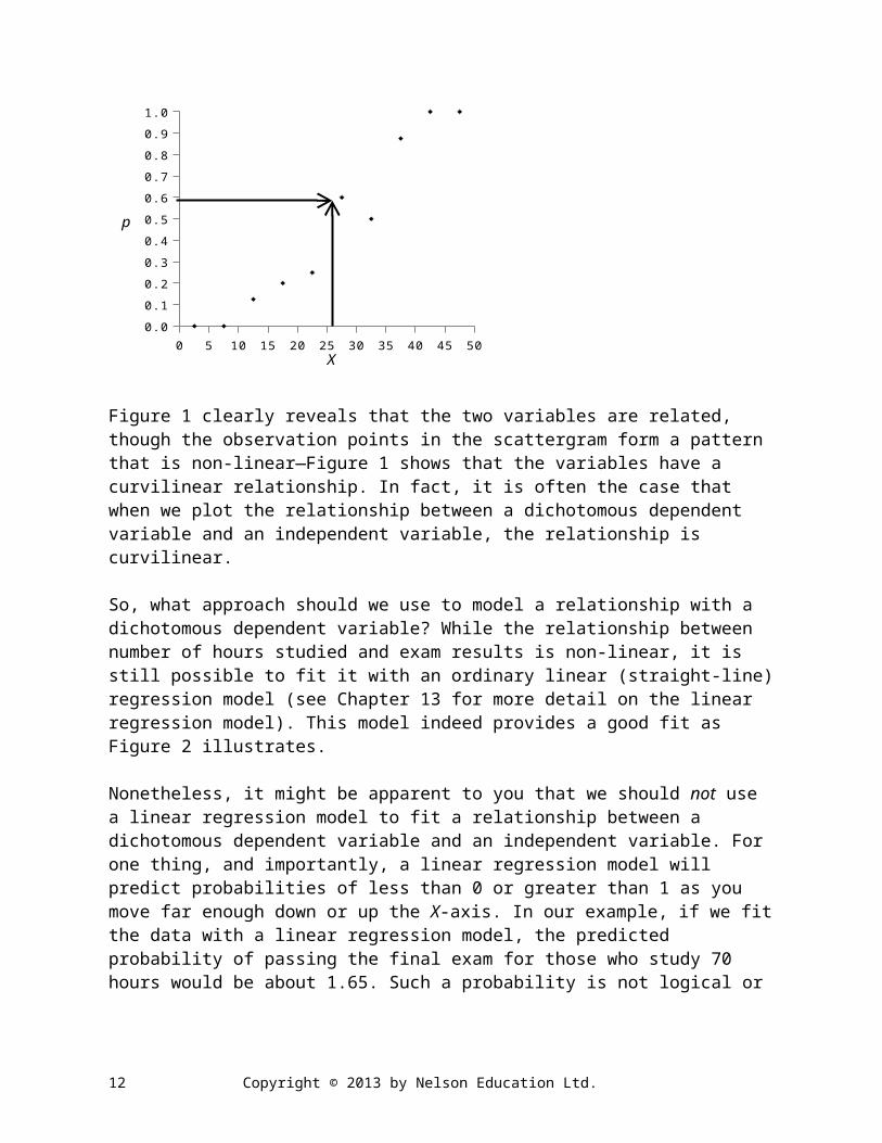
To get a visual sense of the relationship between the two variables in Table 2, Figure 1 plots the data in the form of a scattergram. The figure plots the probability or proportion, p, of observations with the value 1 (pass) on the dependent variable (Y = 1), arrayed along the vertical axis, for each category of the independent variable (hours of study) X, arrayed along the horizontal axis. 4 So, for example, the scattergram points out that the proportion of students that spent between 25 and 29 hours studying for the exam that passed the exam is 0.60. In other words, the probability of passing the exam for those who study between 25 and 29 hours is 0.60. (Remember, proportion and probability of Y = 1 are the same).

2 The interval-width of 5-hours was arbitrarily selected. An interval of another size, such as a 2- or 3-hour interval, could have been just as easily used for this example.3 We also arbitrarily selected the category of interest (Y=1) as “pass.” We could have alternatively coded the dependent variable as 1 for “fail” and 0 for “pass.” As a general rule of thumb, the value coded 1 on the dependent variable should represent the desired outcome or category of “interest” to the researcher.4 It is important to emphasize that we are plotting the proportion of students with the score 1 on the dependent variable from Table 2 and not the actual raw scores of students from Table 1.


Figure 1 Probability of Passing Exam, p, on Hours of Study, X. (Based on data from Table 2).

0 5 10 15 20 25 30 35 40 45 500.0

0.1

0.2

0.3

0.4

0.5

0.6

0.7

0.8

0.9

1.0

X

p

Figure 1 clearly reveals that the two variables are related, though the observation points in the scattergram form a pattern that is non-linear—Figure 1 shows that the variables have a curvilinear relationship. In fact, it is often the case that when we plot the relationship between a dichotomous dependent variable and an independent variable, the relationship is curvilinear.

So, what approach should we use to model a relationship with a dichotomous dependent variable? While the relationship between number of hours studied and exam results is non-linear, it is still possible to fit it with an ordinary linear (straight-line) regression model (see Chapter 13 for more detail on the linear regression model). This model indeed provides a good fit as Figure 2 illustrates.

Nonetheless, it might be apparent to you that we should not use a linear regression model to fit a relationship between a dichotomous dependent variable and an independent variable. For one thing, and importantly, a linear regression model will predict probabilities of less than 0 or greater than 1 as you move far enough down or up the X-axis. In our example, if we fit the data with a linear regression model, the predicted probability of passing the final exam for those who study 70 hours would be about 1.65. Such a probability is not logical or meaningful. Remember, a probability of an event ranges from 0 to 1.


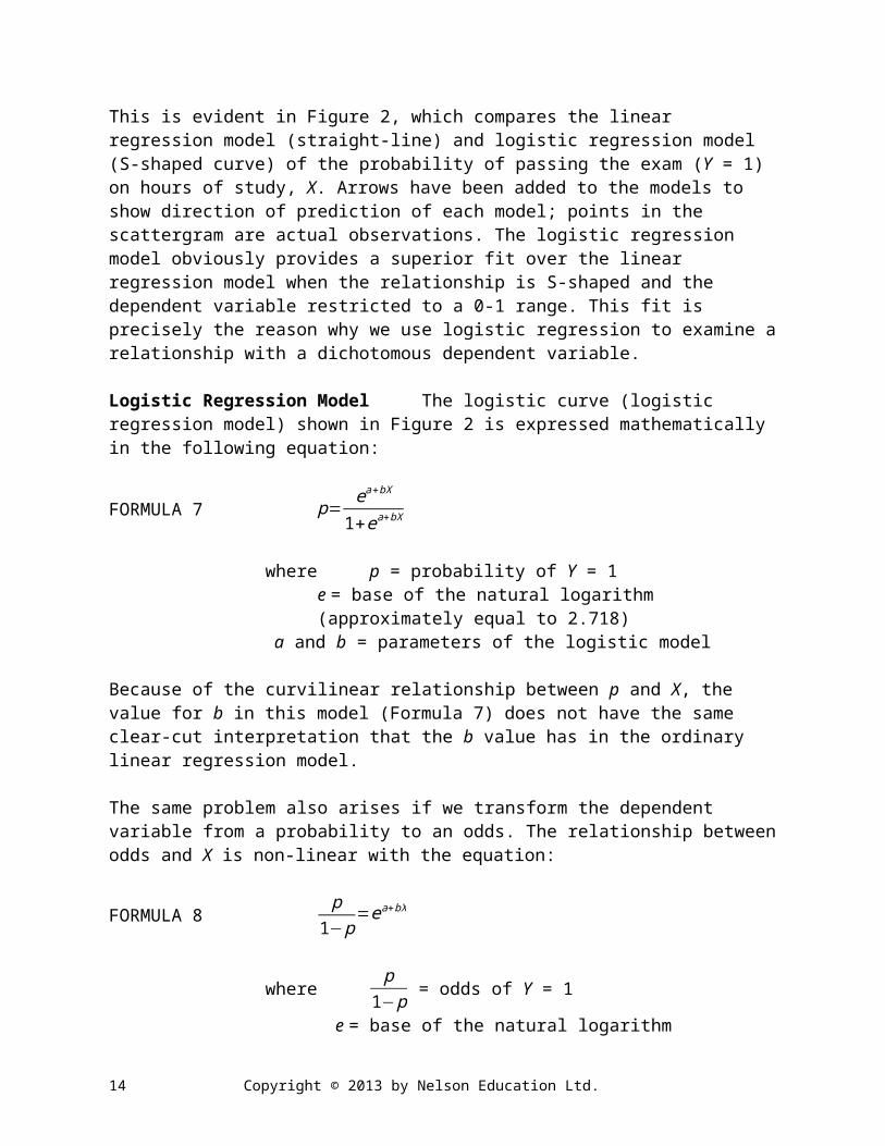
Figure 2 Probability of Passing Exam, p, on Hours of Study, X, with Fitted Linear and Logistic Regression Models. (Based on data from Table 2).

0 5 10 15 20 25 30 35 40 45 50-0.2-0.10.00.10.20.30.40.50.60.70.80.91.01.11.2

X

p

A model called the logistic regression model, on the other hand, uses an S-shaped curve (sometimes referred to as a sigmoid or logistic curve) to fit the relationship between a dichotomous dependent variable and an independent variable. This curve tapers off at 0 on one side and at 1 on the other and thus constrains predicted probabilities to the 0 to 1 range—predicted probabilities are between 0 and 1.

This is evident in Figure 2, which compares the linear regression model (straight-line) and logistic regression model (S-shaped curve) of the probability of passing the exam (Y = 1) on hours of study, X. Arrows have been added to the models to show direction of prediction of each model; points in the scattergram are actual observations. The logistic regression model obviously provides a superior fit over the linear regression model when the relationship is S-shaped and the dependent variable restricted to a 0-1 range. This fit is precisely the reason why we use logistic regression to examine a relationship with a dichotomous dependent variable.

Logistic Regression Model The logistic curve (logistic regression model) shown in Figure 2 is expressed mathematically in the following equation:

FORMULA 7 p= ea+bX

1+ea+bX

where p = probability of Y = 1 e = base of the natural logarithm (approximately equal to 2.718)

a and b = parameters of the logistic model


Linear Regression Model

Logistic Regression Model

Because of the curvilinear relationship between p and X, the value for b in this model (Formula 7) does not have the same clear-cut interpretation that the b value has in the ordinary linear regression model.

The same problem also arises if we transform the dependent variable from a probability to an odds. The relationship between odds and X is non-linear with the equation:

FORMULA 8 p

1−p=ea+bX

wherep

1−p = odds of Y = 1

e = base of the natural logarithm a and b = parameters of the logistic model

There is a way, however, to “linearize” the logistic regression model (i.e., to covert it from an S-shaped model to a straight-line model) so that the b coefficient in this model has the same straightforward interpretation as it does in ordinary linear regression. We linearize the logistic regression model by transforming the dependent variable from a probability to a logit (log odds). This transformed logistic regression model is represented with the following equation:

FORMULA 9 ln ( p1−p )=a+bX

where ln ( p1−p ) = log odds (logit) of Y = 1

a and b = parameters of the logistic model

The logit,ln ( p1−p ), is therefore called a link function since it provides a linear transformation

of the logistic regression model. More specifically, the log transformation of the probability values allows us to create a link with the ordinary linear regression model. Logistic regression is thus considered a “generalized” linear model.

Continuing with our example data from Table 2, Figure 3 summarizes this transformation. Each graph illustrates the shape of the relationship between the independent variable and dependent variable, along with the equations that produce each graph. As we convert probabilities to logits, the relationship transforms from an S-shaped curve to a straight line and the range of values changes from 0 to 1 for probabilities to -∞ to +∞, negative infinity to positive infinity, for logits.


Figure 3 Logistic Regression of Predicted Probability (Graph A), Predicted Odds (Graph B), and Predicted Logit (Graph C) of Passing Exam on Hours of Study, X. (Models fitted from data in Table 2).

Graph A Graph B Graph C

p= ea+bX

1+ea+bX p

1−p=ea+bX ln ( p

1−p )=a+bX

0 10 20 30 40 500.00.10.20.30.40.50.60.70.80.91.0

X

prob

abili

ty

0 10 20 30 40 500

5

10

15

20

25

30

35

40

XO

dds

0 5 10 15 20 25 30 35 40 45 50-5

-4

-3

-2

-1

0

1

2

3

4

5

X

Logit


Given that the relationship between X (independent variable) and the log odds or logit

(dependent variable) is now linear (i . e . ,l n( p1−p )=a+bX), the a and b coefficients in the

logistic regression model are interpreted following the same logic used when interpreting ordinary linear regression coefficients, but taking into account that the quantity represented on the left-hand side of the equation is the log odds (logit) of dependent variable and not the dependent variable itself as it is in ordinary linear regression.

More specifically, as discussed in Chapter 13 of your textbook, the b, or slope coefficient, in ordinary linear regression is interpreted as the amount of change predicted in the dependent variable for a one-unit change in the independent variable—the slope is expressed in the units of the dependent variable. In logistic regression, the slope coefficient, b, is interpreted in the same way, except the dependent variable is measured in log odds, so b tells us the amount of change in the predicted log odds for a one unit change in the independent variable. Likewise, just as the intercept (or constant), a, in the ordinary linear regression model tells us the value of Y when X is zero, the a coefficient in the logistic regression model tells us the value of the log odds when X is zero.

Estimating the Logistic Regression Model Since the logistic regression model has been linearized, it may be tempting to use the least-squares method used in ordinary linear regression (again, see Chapter 13) to obtain estimates of the a and b parameters in the logistic regression model (Formula 9). Instead, for reasons we will not consider here, the parameters a and b are commonly estimated (by many statistical software packages including SPSS) by a method called “maximum likelihood estimation.”

Maximum likelihood estimation is a way of finding the smallest possible difference between the observed and predicted values. It uses a complex iteration, or some other similar numerical, process to find different solutions until it finds the one with the smallest possible difference. It should be pointed out that in many situations there is little difference between the results of the two estimation methods, and in certain cases, ordinary least-squares estimation and maximum likelihood estimation produce the same estimates.

Assumptions of Logistic Regression Logistic regression fortunately does not make many of the assumptions of ordinary linear regression such as normality and homoscedasticity. Nonetheless, a few key assumptions of logistic regression need to be met:

1. the dependent variable must be a dichotomous (dummy) variable with just two values. (Note that a closely related method, called multinomial logistic regression, allows for more than two categories on the dependent variable. Multinomial logistic regression can be thought of as running a series of logistic regression models, where the number of models is equal to the number of categories minus 1. We will not consider this method here).

2. the logit is linearly related to the independent variable. (Note, the independent and dependent variables do not have to be linearly related; the independent variable must be related linearly to only the log odds).


3. the observations must be independent from each other.

4. there should little multicollinearity—the independent variables should be independent from each other.

A Second Look at Logistic Regression

Let’s take another look at logistic regression by considering a hypothetical example of a university that received 900 applications for admission to its school. Table 3 below provides information about the applicants on their overall high school average (HS average), X, and whether or not they were offered admission to the university (admission), Y, coded as 1 for “yes” and 0 for “no.” 5 As we did in our previous example, we again group the independent variable into categories. 6 As a result, we calculate the proportion of applicants with a 1 or “yes” (p of Y = 1) for each level of the independent variable, X, as shown in Table 3, as well as the associated odds and log odds (logits) of Y = 1.

Table 3 High School Average, X, University Admission, Y, and Probability, Odds, and Log Odds of Y = 1 for each Category of X.

X(HS average)

Y(admission

)n

(number of observations)

p(Y = 1)

Odds(Y = 1)

Logit(Y = 1)0 1

(no) (yes)1. <60 60 40 100 0.40 0.67 -0.412. 60-64 59 41 100 0.41 0.69 -0.363. 65-69 50 50 100 0.50 1.00 0.004. 70-74 37 63 100 0.63 1.70 0.535. 75-79 33 67 100 0.67 2.03 0.716. 80-84 21 79 100 0.79 3.76 1.327. 85-89 20 80 100 0.80 4.00 1.398. 90-94 10 90 100 0.90 9.00 2.209. 95+ 8 92 100 0.92 11.50 2.44

5 The way the categories of a dependent variable are coded affects the direction and sign of the logistic regression coefficients. The results will differ depending on whether admission is coded as 1 for “yes” and 0 for “no” vs. coded as 1 for “no” and 0 for “yes.” As previously mentioned, the value coded 1 on the dependent variable should represent the desired outcome or category of “interest” to the researcher.6 We again emphasize that it is just as appropriate to use logistic regression to analyze a relationship using the actual raw ungrouped scores of the independent variable. In our hypothetical example, the raw scores (not shown here) would be the applicants’ actual HS grade-point average. The independent variable is grouped into categories in this example simply for ease of demonstration.


Since the dependent variable is a dichotomous dummy variable, we will use logistic regression to examine the relationship between HS average and admission. Of course the most practical way to conduct a logistic regression is to use specialized software such as SPSS. Thus, Table 4 provides an excerpt of the output for a logistic regression on the data in Table 3. The SPSS output contains more information than shown here, though for our purposes the most important statistics are provided in this table. 7

Table 4 SPSS Logistic Regression Output of Admission on HS Average, X.

B S.E. Wald df Sig. Exp(B)X (HS average) .367 .033 123.284 1 .000 1.443

Constant -.986 .160 37.958 1 .000 .373

Log Odds Ratio Recall that the transformed logistic regression model is expressed in the

equation: ln ( p1−p )=a+bX . Using the results in Table 4, we can write the equation for our

example data as ln ( p1−p )=−.986+.367 X . (SPSS puts the a and b logistic regression

coefficients in the column labeled “B”).

Just like ordinary linear regression, we can use the logistic regression model to make predictions of the dependent variable—to predict log odds of the dependent variable having a value of 1. Furthermore, these logistic regression coefficients are interpreted in the same way as the regression coefficients in ordinary linear regression, except that they are measured in units of log-odds (on the logit scale).

So, the constant or intercept a is the point on the Y-axis crossed by the regression line when X is 0. In the present example, the coefficient for the constant, -0.986, is the predicted log odds of being offered admission to the university when an applicant has a HS average of zero. Since the a coefficient often has very little practical interpretation, we will not consider it further.

Much more useful is the slope coefficient b. We interpret the slope b as the amount change in the predicted log odds that Y = 1 for each one-unit change in X. Thus, b is the log of the odds ratio since it compares the log odds for one unit to the next unit of the independent variable.

7 In the SPSS logistic regression command, the dichotomous dependent variable is regressed on an independent variable, which is treated the same way as it is in ordinary linear regression —an interval-ratio independent variable is entered directly into the logistic regression analysis while nominal and ordinal independent variables are treated as dummy variables and entered together as a group into the analysis. A notable difference is that the SPSS logistic regression command will create dummy variables for you while—as we saw in the “Linear Regression with Dummy Variables” chapter—you must first manually create dummy variables using the SPSS recode command before you run the SPSS ordinary linear regression command.


In our example, we interpret the slope coefficient, 0.367, as the amount of change in the predicted log odds of admission to the university when HS average is increased by one unit. So, as we move-up one category to the next on the HS average scale—for example from category 4 (i.e., HS average of 70 to 74; see Table 3) to category 5 (75 to 79)—the predicted log odds of admission increase by 0.367. 8 Again, since we are comparing the log odds for one unit to the next of the independent variable the slope coefficient b is the log odds ratio.

Next, we will want to know if the coefficient is statistically significant. The “Wald” statistic is used to test the significance of the coefficients in the logistic regression model, and is calculated as follows:

FORMULA 10 Wald statistic=( coefficientSE of coeficient )

2

where SE = Standard Error

So, for the b coefficient in our example:

Wald statistic=( 0 .3670 .033 )

2

=123

Each Wald statistic is compared with a chi-square distribution with 1 degree of freedom, df, though it is more convenient to assess the Wald statistic by looking at the significance value in the column labelled “Sig.” as shown in Table 4. If the value is less than 0.05, we reject the null hypothesis that the variable does not make a statistically significant contribution. The sig. value of .000 for HS average in Table 4 tells us the probability that the observed relationship between HS average and admission occurred by chance alone is very low.

Odds Ratios (OR) Of course, the b coefficient is not very intuitive as it is in units of log odds. The usual method of interpreting b in logistic regression analysis is to take its antilog, the odds ratio, since it is easier to understand effects on the “odds” scale than the “log odds” scale. (See the discussion at the beginning of this chapter for more information on the odds ratio). By getting rid of the log, the logit becomes an odds. What is more, as we will see later, while the log odds ratio, b, gives the additive (i.e., linear) effect on the logit, the odds ratio gives the multiplicative effect on the odds.

We get the odds ratio by exponentiating b—the odds ratio is the exponent of the slope, or e raised to the exponent (power) of b. It is often written as exp(b) or eb. Recall that e, the base of the natural logarithm, is equal to approximately 2.718.

So, in our example where b = 0.367, eb is:

eb¿2.7180.367 = 1.443

8 Hypothetically speaking, had the slope coefficient b been a negative value, -0.367, we would say that the predicted log odds of admission decrease by 0.367. Thus, when b>0 the log odds increase and decrease when b<0.


That is, the odds ratio (OR) is 1.443.

You can find the value of e raised to an exponent using most standard calculators. The e function key typically looks like e* or ex on scientific calculators. To find this value, first enter your exponent in the calculator, then press the e* or ex key. However, SPSS conveniently reports this value, the odds ratio, in the column in labelled "Exp(B).” (See Table 4).

By converting the b coefficient to an odds ratio (OR) we find out how much the predicted odds of Y =1 (the dependent variable having a value of 1) change multiplicatively with a one-unit change in the independent variable, X. In other words, the odds ratio is simply the ratio of the odds at any two consecutive values of the independent variable. We can write this statement as:

OR = ratio the odds of Y = 1 at X +1 and odds of Y = 1 at X, for all values of X

In our example, the odds ratio is 1.443, which we will round off to 1.4 for convenience. Therefore, the predicted odds of admission to the university for applicants with a HS average of 60 to 64 are 1.4 times as large as the predicted odds for applicants with a HS average of <60; the predicted odds for applicants with a HS average of 65 to 69 are 1.4 times as large as the predicted odds for applicants with a HS average of 60 to 64; the predicted odds for applicants with a HS average of 70 to 74 are 1.4 times as large as the predicted odds for applicants with a HS average of 65 to 69; and so on. Hence, the predicted odds increase in a multiplicative fashion—they are 1.4 times as large—with each unit increase in the independent variable. 9 10

To further illustrate how a change in a unit of X multiplies the predicted odds by 1.4, consider the respective predicted odds of admission for an applicant with a HS average of <60 (category 1 in Table 3), 60-64 (category 2), 65-69 (category 3), and 70-74 (category 4) (note that to calculate predicted odds we use Formula 8, odds=ea+bX):

Predicted Odds for Category 1=e−0.986+0 .367(1)=2.718−0.619=0.538Predicted Odds for Category 2=e−0.986+0 .367(2)=2.718−0.252=0.777Predicted Odds for Category 3=e−0.986+0 .367 (3)=2.7180.115=1.122

9 If you prefer, you can subtract 1 from the odds ratio and multiply by 100 to get the percent change in odds (i.e., for a one-unit increase in X, we expect to see a % increase in the odds of the dependent variable). So, in our example, we can say either “the predicted odds of admission are about 1.4 times higher with each unit increase in HS average” or “the predicted odds of admission are about 40%— (1.4-1.0)*100 = 40% —higher with each unit increase in HS average.” These descriptions are equal, so is it your choice which style you use to report the results. 10 The odds ratio, eb, has a simpler interpretation in the case of a nominal or ordinal (i.e., dummy) independent variable. In this case the odds ratio represents the odds of having the characteristic of interest (Y = 1) for one category compared with the other. Let’s say, for instance, that we are interested in the relationship between sex, X, and admission, Y, where sex is coded as 1 for “female” and 0 for “male.” If eb = 1.09, we would interpret this value as: the odds of admission are 1.09 times (or 9%) greater for a female applicant than for an applicant who is male.


Predicted Odds for Category 4=e−0.986+0 .367(4 )=2.7180.482=1.619

So, the predicted odds of admission for those in category 2 (HS average of 60 to 64) and category 1 (HS average of <60) are 0.777 and 0.538 respectively, giving an odds ratio of1.4. Recall, from Formula 3, the odds ratio (OR) is:

¿=odds2

odds1=0.777

0.538=1.4

Next, the predicted odds of admission for those in category 3 (HS average of 65 to 69) and category 2 (HS average of 60 to 64) are 1.122 and 0.777 respectively, giving an odds ratio of 1.4 :

¿=odds3

odds2=1.122

0.777=1.4

Next, the predicted odds of admission for those in category 4 (HS average of 70 to 74) and category 3 (HS average of 65 to 69) are 1.619 and 1.122 respectively, giving an odds ratio of1.4:

¿=odds4

odds3=1.619

1.122=1.4

and so on. Therefore, an odds ratio of 1.4 means that the odds increase by 1.4 no matter the values of the independent variable—going from any value of the independent to the subsequent value of the independent will always increase the odds by a factor of 1.4.

This multiplicative effect, such that the ratio of any odds to the odds in the next category is constant, is graphically illustrated in Figure 4. The figure shows the logistic regression of predicted odds of admission on HS average. The model (odds=e−0.986+0 .367 X ¿ is fitted from data in Table 3—the predicted odds are marked with the symbol *, with the logistic regression model superimposed through them. For comparative purposes, the observed odds (□) taken from Table 3 are also plotted. Importantly, note that the general shape of the relationships between the independent variable and dependent variable is the same in both Figure 4 and Graph B in Figure 3. Both graphs show the change in odds on a multiplicative scale.


Figure 4 Logistic Regression of Predicted Odds of Admission on HS Average, X. (Model fitted from data in Table 3). odds=e−0.986 +0 .367X

0 1 2 3 4 5 6 7 8 9 100

3

6

9

12

15

Observed Odds Predicted Odds

X

odds

As a final comment, note the following relationships between b, eb (odds ratio), odds, and probability:

1. (b =0) = (eb =1) = odds and probability are the same at all X levels2. (b <0) = (eb <1) = odds and probability decrease as X increases 3. (b >0) = (eb >1) = odds and probability increase as X increases

Back to Probabilities In logistic regression, we can interpret the results not only in terms of predicted log odds or odds of Y = 1, but also in terms of predicted probabilities of Y = 1. In the previous section we saw how to transform the logit back to an odds using Formula 8 (odds=ea+bX ¿ . Once we have converted from log odds to odds, we can easily convert the odds

back to probabilities using Formula 7 (p= ea+bX

1+ea+ bX ).

Let’s consider the following example for X = 1 in the present example (i.e., category 1 in Table 3 or an applicant with a HS average of <60):

the predicted log odds would be: ln ( p1−p )=−.986+.367(1)=−.986+.367 = -0.619;

the corresponding predicted odds would be: odds=ea+bX=2.718−0.986+ 0.367 (1)=0.538;

and finally, the corresponding predicted probability would be: p= ea+bX

1+ea+ bX = 0.5381+0.538

=0.350


If you perform this conversion to probabilities throughout the range of X values, you go from the straight line of the logit to the S-shaped curve of p as revealed in Figure 5. Again notice the general shape of the relationships between the independent variable and logit is the same in both the top graph of Figure 5 and Graph C in Figure 3—both graphs are linear—and that the general shape of the relationships between the independent variable and probability is the same in both the bottom graph of Figure 5 and Graph A in Figure 3—both graphs are S-shaped.

We should finally point out that the model provides a “good fit.” For example, the predicted probability for X = 1 of 0.35 is fairly close in value to the observed probability of 0.40. Comparison of the observed to predicted values from the fitted models in Figure 5 suggests that the models provide an overall good fit.

Figure 5 Logistic Regression of Predicted Logit and Predicted Probability of Admission on HS Average, X. (Models fitted from data in Table 3)

ln ( p1−p )=a+bX

0 1 2 3 4 5 6 7 8 9 10-1.5

-1.0

-0.5

0.0

0.5

1.0

1.5

2.0

2.5

Observed Logits Predicted LogitsX

logi

t

p= ea+bX

1+ea+bX


0 1 2 3 4 5 6 7 8 9 100.2

0.3

0.4

0.5

0.6

0.7

0.8

0.9

1.0

Observed Probabilities Predicted ProbabilitiesX

prob

abili

ty


· web viewlogistic regression shares the same objective as linear regression. logistic and linear...

Documents