AAE 451SPRING 2006

PRELIMINARY DESIGN REVIEW

TEAM 03THE HYDROGEN BUSINESS JET

DEREK DALTONMEGAN DARRAUGH

SARA DAVIABEAU GLIMSETH HAHN

LAUREN NORDSTROMMARK WEAVER

Executive Summary

As businesses expand to new markets overseas, the need for business executives to have an aircraft capable of transoceanic flight at a moments notice becomes even more important. The Hydrogen Business Jet (HBJ), a hydrogen fueled, ultra-long-range aircraft, adequately fulfills this growing need even after kerosene-fuelled aircraft are no longer a viable option.

The properties of hydrogen vary significantly from any other kerosene-based fuel and as such, designing a hydrogen-fuelled aircraft presents a few new challenges to overcome before a preliminary design is complete. The cryogenic storage systems required to store hydrogen as a liquid as well as hydrogen’s low density change the HBJ’s fuel storage systems significantly.

Changes in the fuel system make it difficult to incorporate an off-the-shelf engine into the design of the HBJ. Thermodynamic analysis of a twin-spool turbofan engine creates an engine specifically tailored to meet the design requirements of the HBJ. The designed engine produces 33,000 lbs of thrust at sea level static conditions and is capable of providing the required thrust at the cruise altitude of 40,000 ft.

Estimates of the cost of the HBJ use a regression of published business jet data that related empty weight, range, and cruise Mach number to acquisition cost. The empirically derived equations for predicting the cost of an aircraft require modification to include the new systems that a hydrogen fuel necessitates. A scaling factor accounts for the additional costs of the new hydrogen systems and the HBJ a preliminary estimate of the acquisition cost is $62 million.

FLOPS, a NASA-developed aircraft sizing program, was modified to preliminarily size the HBJ by using the many override parameters built into the program. FLOPS uses initial estimates of thrust-to-weight, aspect ratio, and wing loading to calculate the gross takeoff weight but further revision of the input parameters is necessary.

A method of constrained carpet plots use the maximum fuel capacity and landing field length constraints to further refine the input values of FLOPS. The external dimensions of the Boeing Business Jet set the external size of the HBJ. These dimensions allow the HBJ to remain flexible enough to service the business executive needs while still holding enough hydrogen to make a nonstop flight from Los Angeles to Tokyo. The new values are used to calculate the final preliminary design values for the HBJ. Current estimates of the main aircraft characteristics are as follows:

GTOW 58,700 lb Acquisition Cost $62 million Range 5,700 nmi Cruise Speed 0.80 Mach Wing Span 83.5 ft Overall Length 123 ft

Table of Contents

Table of Contents............................................................................................................................iTable of Equations.........................................................................................................................iiTable of Figures............................................................................................................................iiiTable of Tables..............................................................................................................................ivMarket Overview and Design Requirements..............................................................................1Present Concept.............................................................................................................................2

Design Schematic.......................................................................................................................2Volumetric Analysis...................................................................................................................3FLOPS Sizing Analysis..............................................................................................................5

Constraint Analyses.......................................................................................................................6Mission Analysis.........................................................................................................................9Takeoff and Landing Distances..............................................................................................10

Aerodynamics...............................................................................................................................11Performance.................................................................................................................................13

Flight Performance Envelope.................................................................................................13Placard Diagram......................................................................................................................14V-n Diagram.............................................................................................................................15

Structures.....................................................................................................................................16Materials...................................................................................................................................16Landing Gear...........................................................................................................................18Wing Spar.................................................................................................................................18

Balance and Stability...................................................................................................................19Center of Gravity.....................................................................................................................20Static Margin............................................................................................................................21Vertical Tail Sizing..................................................................................................................22

Engine Design and Performance................................................................................................23Modifications............................................................................................................................23Engine Design...........................................................................................................................23

Cost................................................................................................................................................28Summary......................................................................................................................................31

Outstanding Issues...................................................................................................................33Structures.............................................................................................................................33Aerodynamics.......................................................................................................................33Balance and Stability...........................................................................................................33

References.....................................................................................................................................34

Appendix 1: Wing Spar Calculations........................................................................................A1Appendix 2: Cost.........................................................................................................................A2Appendix 3: FLOPS Input.........................................................................................................A4Appendix 4: Balance and Stability............................................................................................A5

Neutral Point...........................................................................................................................A7Appendix 5: Carpet Plot Code.................................................................................................A10Appendix 6: Engine Design......................................................................................................A15

Density and Temperature Functions...................................................................................A15Flight Envelope Matlab code...............................................................................................A16Engine Cycle Equations........................................................................................................A18

Station ∞ 1 (inlet):.........................................................................................................A18Station 1 2 (fan compression):.......................................................................................A18Station 2 8 (fan nozzle):.................................................................................................A18Station 1 3 (compressor):...............................................................................................A18Station 3 4 (combustor):................................................................................................A18Station 4 5 (high pressure turbine):................................................................................A19Station 5 6 (low pressure turbine):.................................................................................A19Station 6 7 (core flow nozzle):.......................................................................................A19Thrust and SFC:..................................................................................................................A19

Engine Cycle code.................................................................................................................A20Appendix 7: Configuration Trade Studies..................................................................................A22

Table of Equations

Equation 1: Calculated Engine Thrust...........................................................................................13Equation 2: Trend-Based Cost Estimate........................................................................................28Equation 3: Tail Area as a Function of Force...............................................................................A5Equation 4: Static Margin.............................................................................................................A7Equation 5: Neutral Point.............................................................................................................A7Equation 6: Horizontal Tail Volume Coefficient.........................................................................A7Equation 7: Yaw Coefficient........................................................................................................A8

Table of Figures

Figure 1: The Hydrogen Business Jet..............................................................................................2Figure 2: Fuel Tank Layout.............................................................................................................3Figure 3: Landing Constraint Diagram............................................................................................7Figure 4: Overall Constraint Diagram.............................................................................................7Figure 5: Aspect Ratio Constraint Diagram....................................................................................8Figure 6: Design Mission.................................................................................................................9Figure 7: Required Field Length....................................................................................................10Figure 8: Drag Polar for Various Mach Numbers.........................................................................11Figure 9: Conventional and Supercritical Airfoil Pressure Distributions......................................12Figure 10: Aerodynamic Flight Envelope.....................................................................................13Figure 11: Placard Diagram...........................................................................................................14Figure 12: V-n diagram at 28,000 ft..............................................................................................15Figure 13: Structural Layout..........................................................................................................16Figure 14: Hydrogen Tank Structure.............................................................................................17Figure 15: Center of Gravity Location Travel...............................................................................20Figure 16: Moment Diagram (One Engine Out)............................................................................22Figure 17: Sketch of Engine Cycle with Station Numbers............................................................23Figure 18: Fan Study for Sea Level Static.....................................................................................25Figure 19: Fan Study for Cruise Conditions..................................................................................25Figure 20: Total Pressure Ratio Study for Varying Bypass Ratios...............................................26Figure 21: Thrust vs. Mach Number for Varying Altitudes..........................................................27Figure 22: RDT&E Cost Breakdown............................................................................................30Figure 23: Center of Gravity Location for Aircraft Major Components......................................A5Figure 24: Stability Locations.......................................................................................................A8Figure 25: Passenger Cabin Layout..............................................................................................A9Figure 26: Density as a Function of Altitude..............................................................................A15Figure 27: Temperature as a Function of Altitude......................................................................A15Figure 28: Modified Hydrogen Engines.....................................................................................A17Figure 29: Trade Study Fuel Locations......................................................................................A22

Table of Tables

Table 1: Current Design Requirements...........................................................................................1Table 2: Fuel Tank Properties..........................................................................................................3Table 3: FLOPS Input Parameters...................................................................................................5Table 4: Design Constraints on HBJ...............................................................................................6Table 5: Landing Field Length for Various T/W and W/S..............................................................6Table 6: Mission Performance.........................................................................................................9Table 7: Takeoff and Landing Distances.......................................................................................10Table 8: V-n Diagram Output........................................................................................................15Table 9: Material Selection for Critical Sections..........................................................................16Table 10: Landing Gear Tire Sizes................................................................................................18Table 11: Spar Dimensions............................................................................................................18Table 12: Weight Breakdown........................................................................................................19Table 13: Tank Weight Distribution..............................................................................................19Table 14: Static Margin.................................................................................................................21Table 15: Vertical Tail Sizing........................................................................................................22Table 16: Typical Process Efficiencies..........................................................................................24Table 17: HBJ Turbofan Predictions Comparison to Cryoplane Data..........................................24Table 18: Final Parameters for HBJ Twin Spool Turbofan...........................................................27Table 19: HBJ Acquisition Cost Trade Study...............................................................................28Table 20: RDT&E Cost Trade Study.............................................................................................29Table 21: Acquisition Cost and DOC for HBJ and Competitors...................................................29Table 22: Comparison of HBJ and Competing Aircraft................................................................31Table 23: Weight Fraction Comparison........................................................................................32Table 24: Wing Spar Calculations................................................................................................A1Table 24: DOC Outputs................................................................................................................A2Table 25: DOC Inputs...................................................................................................................A2Table 26: RDT&E Cost Inputs.....................................................................................................A3Table 27: RDT&E Cost Breakdown.............................................................................................A3Table 28: HBJ Parameters............................................................................................................A6Table 29: Individual Component Weight & Center of Gravity Location.....................................A6Table 30: Federal Aviation Regulations.......................................................................................A9Table 31: Assumed Process Efficiencies for Engine Cycle........................................................A17Table 32: Combustion Calculuation Values...............................................................................A18Table 33: C.G. Location Trade Study.........................................................................................A23Table 34: Static Margin Trade Study Values..............................................................................A23

1

Market Overview and Design Requirements

The Hydrogen Business Jet (HBJ) is a non-petroleum-fuel-based, medium-capacity, ultra-long-range business jet. Liquid hydrogen fuel best satisfies the design requirements presented in Table1 due to its low specific fuel consumption (SFC) and high specific energy. Catering to the needs of the business elite, the aircraft provides lavish accommodations for eight passengers during flights up to thirteen hours in duration; a flight between Los Angeles and Tokyo is the representative design mission. Worldwide increases in demand within the ultra-long-range business aircraft market, and the global nature of business, require that companies absorb cost increases arising from depleted fossil fuel reserves, making high-valued corporations a captive market for this product. With 10-year revenues in the entire ultra-long-range market projected to exceed $50 billion (2006 dollars), capturing a 25% market share would provide $1.25 billion in annual sales, or 4% of the total business aviation market1. Capturing this market share corresponds to selling approximately 20 $62 million aircraft per year. Assuming 10% profit from each aircraft sold and a total of $12 billion in development costs, it is possible to break even in 2050, 10 years after the planned market entry

Table 1: Current Design Requirements

In addition to the range, passenger capacity, and cruise speed requirements, adding a cruise altitude constraint of 40,000 ft allows the HBJ to remain competitive. The range and cruise speed requirements enable a maximum flight endurance of approximately 13 hours. Federal Aviation Requirements (FARs) mandate that no flight crew operate an aircraft for longer than 12 hours, and the HBJ accordingly accommodates two separate flight crews for its design range mission. Having discussed the mission requirements, a detailed discussion of the aircraft is next on the agenda.

Hydrogen is the best non-petroleum-based fuel to fulfill the HBJ’s design requirements because it lacks the harmful emissions present in conventional fuels (its only emission is water) and has a high specific energy. These attributes provide the lowest possible gross takeoff weight among the alternative fuels considered (biodiesel, liquid hydrogen, and liquid methane) by significantly lowering the weight of fuel required to meet the design range.

2

Present Concept

Design Schematic

Figure 1: The Hydrogen Business Jet

The Hydrogen Business Jet functions as a mid-capacity, ultra-long-range executive transport. However, because of a significant increase in fuel storage volume required to contain all of the liquid hydrogen, the external size of the aircraft is equivalent to a Boeing 737-500. The aircraft is 123 ft in length and has a wingspan of 84 ft. An elliptical fuselage with a major axis diameter of 12 ft and a minor axis diameter of 8 ft best contains both fuel and passengers; however, to reduce complexity, a pressurized circular section comprises the passenger cabin (Figure 2 presents a more detailed representation of the fuselage). The upper-right isometric figure in Figure 1 displays the fuel tank layout in relation to the passenger cabin2.

The long duration of the HBJ’s design mission and customer expectations require a lavish interior suited to productivity and privacy. Though capable of carrying up to twelve passengers, the design mission accommodates eight passengers to maximize comfort. The current configuration includes an extended crew section to accommodate the off duty, resting crewmembers (5.5 ft), also, the lavatory is located in the rear of the cabin because passengers value privacy in the location of the lavatory more than preventing the intrusion of crew into the passenger cabin during flight.

3

Volumetric Analysis

The greatest hurdle in determining the size of a hydrogen-fueled aircraft lies in determining where to place the fuel. Fixing the maximum fuselage length threshold to the length of the Boeing Business Jet (BBJ), one of the largest ultra-long-range business jets in the market, establishes the maximum amount of fuel at 11,700 lbs. With the nose, tail, and passenger cabin already sized, all remaining interior space was filled with fuel (see Interior Design in Appendix 4). Limiting external dimensions allows the HBJ to maintain a consistent size with the BBJ. Several considerations limit the HBJ’s dimensions: the desire to maintain consistency within the market’s size distribution; customer requirements for aircraft flexibility (e.g. hangar size and runway length); and, primarily, minimizing the surface area surrounding the fuel tanks and passenger cabin (presented below). These considerations combine to produce an aircraft slightly smaller than the BBJ, which will easily fit in standard hangars and provide the customer with the necessary airport flexibility.

Figure 2: Fuel Tank Layout

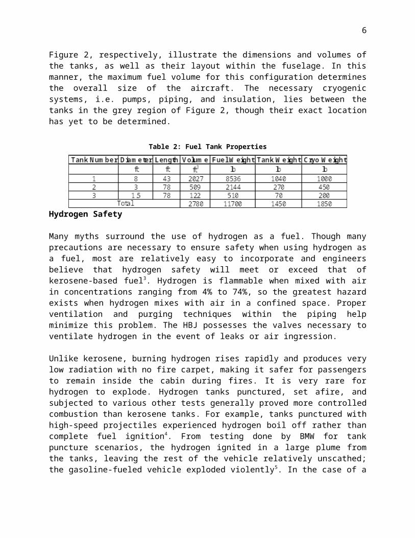
A ten-tank layout maximizes the space available for fuel while minimizing the problems associated with regulating temperature and pressure throughout overly large pressure vessels. This layout consists of three large, 3 ft diameter tanks and six smaller, 1.5 ft diameter tanks running above the passenger cabin along the length of the fuselage, with the largest, eight-foot diameter tank located behind the passenger cabin. Table 2 and Figure 2, respectively, illustrate the dimensions and volumes of the tanks, as well as their layout within the fuselage. In this manner, the maximum fuel volume for this configuration determines the overall size of the aircraft. The necessary cryogenic systems, i.e. pumps, piping, and insulation, lies between the tanks in the grey region of Figure 2, though their exact location has yet to be determined.

Table 2: Fuel Tank Properties

4

Hydrogen Safety

Many myths surround the use of hydrogen as a fuel. Though many precautions are necessary to ensure safety when using hydrogen as a fuel, most are relatively easy to incorporate and engineers believe that hydrogen safety will meet or exceed that of kerosene-based fuel3. Hydrogen is flammable when mixed with air in concentrations ranging from 4% to 74%, so the greatest hazard exists when hydrogen mixes with air in a confined space. Proper ventilation and purging techniques within the piping help minimize this problem. The HBJ possesses the valves necessary to ventilate hydrogen in the event of leaks or air ingression.

Unlike kerosene, burning hydrogen rises rapidly and produces very low radiation with no fire carpet, making it safer for passengers to remain inside the cabin during fires. It is very rare for hydrogen to explode. Hydrogen tanks punctured, set afire, and subjected to various other tests generally proved more controlled combustion than kerosene tanks. For example, tanks punctured with high-speed projectiles experienced hydrogen boil off rather than complete fuel ignition4. From testing done by BMW for tank puncture scenarios, the hydrogen ignited in a large plume from the tanks, leaving the rest of the vehicle relatively unscathed; the gasoline-fueled vehicle exploded violently5. In the case of a hydrogen-fueled aircraft, fuel safety is not an obstacle that prevents further design advances.

5

FLOPS Sizing Analysis

The Flight Optimization System (FLOPS) developed by NASA sized the HBJ, and provided drag estimates, performance values, cost estimations, and various other necessary parameters. FLOPS is a combination of several scripts utilizing empirical formulas originally designed to estimate flight parameters for military aircraft, and the HBJ’s internal fuel storage system necessitated a number of modifications to the typical input file. Inputting the design mission (Figure 6, below) and requirements (Table 1) allows the program to generate a number of ancillary parameters and flight performance tables that a simple sizing code cannot produce.

Some representative FLOPS inputs are enumerated in Table 3, and varying the wing loading, thrust to weight, and aspect ratio generated the values used to determine the minimum thrust-to-weight, takeoff weight, and aspect ratio within the carpet plot studies (see Constraint Analyses).

Historical values from competing aircraft determine the aircraft’s wing sweep and taper ratio. The sweep range for many ultra-long-range aircraft varies from 27° (Gulfstream G550) to 34° (BBJ), so the HBJ has a mid-range sweep of 30°. Existent but limited supercritical airfoil data left little room for modification to the thickness-to-chord ratio, though a more in-depth sizing analysis would likely evidence small changes to both of these values, as expected in any type of aircraft analysis. In order for FLOPS to perform the proper analysis, it was important to input specific engine parameters for detailed drag analysis and weight breakdown. Conducting a separate engine study, discussed in Engine Design and Performance, defined the turbine inlet temperature, pressure ratio, and bypass ratio to allow FLOPS to size the engine.

Table 3: FLOPS Input Parameters

Sizing the HBJ required additional FLOPS modifications, since this aircraft deviates significantly from traditional designs. General modifications include increasing the fuel heating value to account for the use of hydrogen fuel rather than jet fuel and moving the fuel storage location from the wings into ten storage tanks within the fuselage (see Volumetric Analysis). Additional modifications include using composite materials for the wing and scaling some default factors within FLOPS to account for the increase in weight of the fuel systems and airframe structure resulting from the use of cryogenics. Typical increases in cryogenic fuel system weight range from two to eight times the weight of the kerosene fuel system for an equivalent aircraft, and the HBJ uses a scaling factor of five.

6

Constraint Analyses

Using constrained carpet plots produces reasonable values for a number of defining HBJ characteristics, namely gross takeoff weight, landing field length, engine thrust, and the mission’s required fuel weight. The values from Table 1 represent fixed requirements that no design may violate, and are held constant within the FLOPS input file (see Appendix 3).

In order to meet these fixed values, an analysis varies the performance constraints of landing field length, gross takeoff weight, thrust per engine, and fuel weight to allow a trade-off that maximizes the aircraft’s performance. Each constraint serves a specific purpose: reducing landing field length expands the available number of airfields, which increases destination flexibility; gross takeoff limits cost and size; reducing thrust also limits the engine size; and fuel weight limits the external dimensions of the aircraft as discussed in Volumetric Analysis. Notably, the constraints listed in Table 4 do not optimize the HBJ; rather, varying each constraint allows for a marginal analysis (i.e. balancing the cost-benefit relationship).

Table 4: Design Constraints on HBJ

For any given wing loading and thrust-to-weight input, FLOPS generates a value for each of the four design constraints. By incrementing wing loading and thrust to weight in the FLOPS input file and recording the subsequent outputs, a trend emerges within the generated series of points. A constraining trend line emerges from the intersection between the constraint in Table 4 and the corresponding data in Table 5. For example, a wing loading of 105 lb/ft2 results in an acceptable landing field length, but a wing loading of 110 lb/ft2 and above results in unacceptable distances; thus, the constraining trend line for landing field length is within this range.

Table 5: Landing Field Length for Various T/W and W/S

Constraint diagrams for each requirement are generated by plotting a trend line through the set of wing loading values for each of the three thrust-to-weight ratios. The landing field length requirement shown in Figure 3 (as a function of gross takeoff weight) illustrates the HBJ’s maximum allowable wing loading that does not exceed the distance requirement of 5,600 ft.

7

Figure 3: Landing Constraint Diagram

Plotting each of the four constraint conditions (gross takeoff weight, landing field length, engine thrust, and fuel weight) on the same axes generates a single diagram defining the complete allowable design space for the aircraft. In Figure 4, this allowable design space lies within the landing field length and fuel weight limits. The two remaining constraints ultimately proved redundant and hence do not appear in the figure. In the final case shown below, the minimum gross takeoff weight is 58,700 lbs, which occurs at a thrust-to-weight ratio of 0.43.

Figure 4: Overall Constraint Diagram

8

The above method for generating a carpet plot applies to a fixed aspect ratio, but can generate an aspect ratio trade with slight modification. Conducting the above method for a number of different aspect ratios provides a corresponding minimum gross takeoff weight. Plotting these aspect ratios and gross takeoff weights produces a gross takeoff weight versus aspect ratio polynomial regression trend that defines the trade-off balanced aspect ratio. The HBJ’s aspect ratio is 11.9, as indicated by the design point in Figure 5. Completing the trade studies for basic sizing parameters allows for more in depth analyses of the mission and aircraft performance.

Figure 5: Aspect Ratio Constraint Diagram

9

Mission Analysis

For an ultra-long-range mission, the cruise segment consumes the majority of time (92% for the HBJ) and fuel (75%). However, the mission’s climb segment requires the most thrust, 18,800 lbs, and this segment effectively sizes the engine. The climb segment also generates the mission’s maximum lift-to-drag ratio of 17.0, which is similar to predictions made by the European Union’s Cryoplane project for hydrogen-fueled passenger aircraft6. Figure 6 and Table6 show the design mission run in FLOPS for the HBJ along with corresponding values for each segment. The HBJ’s design mission requires approximately 13.5 hours to complete and consumes 11,780 lbs of fuel (including reserves).

Figure 6: Design Mission

Table 6: Mission Performance

10

Takeoff and Landing Distances

The HBJ must be able to meet or best the airport flexibility of similarly ranged aircraft to remain competitive. If the aircraft cannot takeoff or land at a sufficiently large number of airports, its functionality to business executives suffers. The typical takeoff length for the BBJ is approximately 5,700 ft, and this value sets the maximum runway length for the HBJ. Since the HBJ’s gross takeoff weight is significantly less than conventionally fueled counterparts, its takeoff distance is proportionally shorter.

In traditional aircraft, empty weight accounts for approximately 55% of the gross takeoff weight. Due to the low weight of hydrogen, the empty weight fraction of the HBJ is significantly higher (75%). When approaching for landing, the HBJ is proportionally heavier than traditional aircraft because the weight of the consumed fuel is relatively light. A conventional business jet can land in approximately 50% of its takeoff distance, but since a larger proportion of its takeoff weight remains with the HBJ, its landing distance increases to more than 70% of the takeoff field length. Table 7 presents the takeoff and landing distance of the HBJ, as well as the equations used to calculate these values.

Table 7: Takeoff and Landing Distances7

The distinction between field length roll and required field length distance is that ‘roll’ describes the actual field length required by the aircraft in order to stop, whereas ‘distance’ includes a regulatory Factor of Safety (1.67·Sroll). The Result column of Table 7 includes this regulatory factor and represents the maximum dry landing field length required by either the JAA or FAA. For wet landings, additional regulations necessitate a further Factor of Safety (1.92·Sroll). Figure7 illustrates both wet and dry landing scenarios.

Figure 7: Required Field Length

11

Aerodynamics

Design requirements for the HBJ necessitate a detailed aerodynamic analysis to maximize efficiency. The long cruise segment makes drag a particularly important factor; reducing drag by even a few drag points saves a significant amount of fuel and decreases the direct operating costs of the aircraft (see Costs).

A drag polar is one of the best ways to represent the overall drag of an aircraft. The FLOPS output included a section detailing the drag coefficient (CD) at various lift coefficients (CL), and generates a drag polar for the entire aircraft. FLOPS does not allow for an input of the airfoil coordinates, but the overall drag polar provides a good initial estimate of the aircraft’s drag. Figure 8 displays the calculated drag polars for various Mach numbers. FLOPS also calculates the CL required to provide sufficient lift throughout the entire mission, which varies between 0.45 and 0.50. These two values represent flight condition boundaries, illustrated by the two horizontal lines in Figure 8; each curved trend line represents the relationship between the drag and lift coefficients. The drag remains relatively constant as long as the cruise Mach number remains below 0.825 Mach. Once the cruise Mach number crosses this threshold, the wave drag on the aircraft increases and reduces the cruise fuel efficiency. While the aircraft can cruise at 0.90 Mach if necessary, fuel efficiency dictates a design speed of 0.80 Mach.

Figure 8: Drag Polar for Various Mach Numbers

12

The airfoil is one of the most critical aspects in minimizing the drag on the aircraft. Conventional airfoils (NACA 5- and 6-series) do not have the necessary characteristics to keep drag to a minimum for the required transonic cruise speeds. When transonic flow passes over a conventional airfoil, the flow rapidly accelerates near the leading edge. Since the flow already travels at nearly supersonic speeds, it becomes locally supersonic. Shocks form as the flow passes over the airfoil and increase drag. A supercritical (transonic) airfoil keeps drag to a minimum and prevents shocks from occurring by slowly accelerating the flow along the entire chord. Figure 9 shows a comparison between the pressure distribution (which is proportional to a velocity distribution) of a conventional airfoil and a supercritical airfoil. There is no readily available database of supercritical airfoils since most transonic aircraft have airfoils specifically designed to meet their precise mission requirements. To keep the drag on the wing as low as possible, a supercritical airfoil must be designed to meet the requirements of the HBJ. These requirements include the capability to produce CLcruise of 0.5 or higher, CLmax of 1.8, and a lift-to-drag ratio between 14 and 17.

Figure 9: Conventional and Supercritical Airfoil Pressure Distributions

13

Performance

Having defined the dimensions of the aircraft, three separate performance envelopes determine the flight safety limits: a flight envelope, a Placard diagram, and a V-n diagram. The diagrams aid in the analysis of the HBJ performance parameters. The flight performance envelope is a closed area that specifies the operating conditions of an aircraft, whereas the Placard diagram is shows the structural design airspeeds as a function of altitude. Lastly, the V-n diagram displays the envelope where the aircraft is structurally capable of flying under various loading conditions.

Flight Performance Envelope

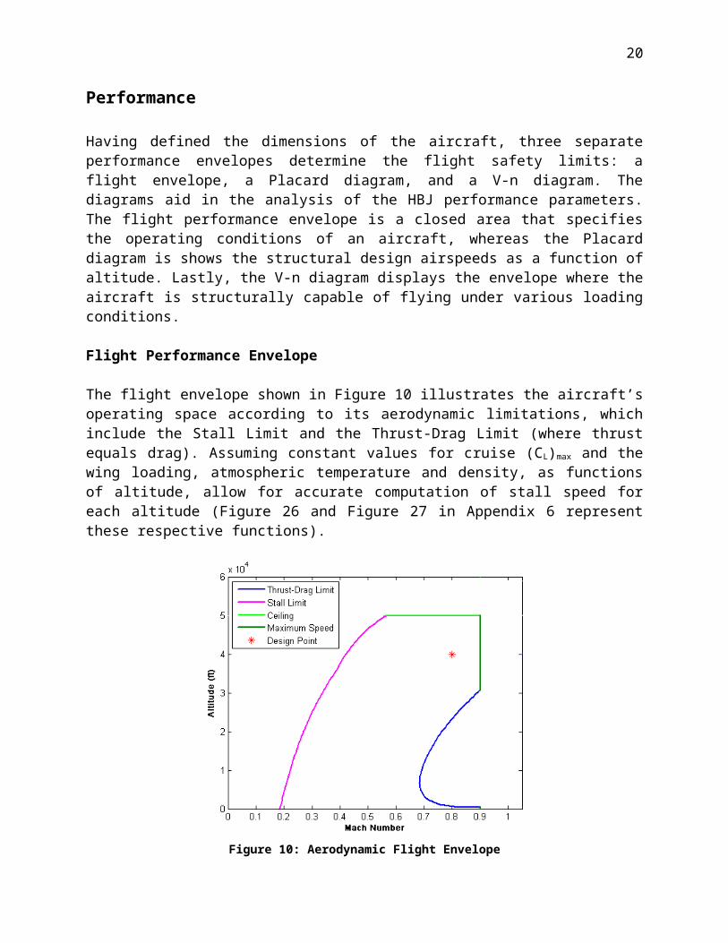
The flight envelope shown in Figure 10 illustrates the aircraft’s operating space according to its aerodynamic limitations, which include the Stall Limit and the Thrust-Drag Limit (where thrust equals drag). Assuming constant values for cruise (CL)max and the wing loading, atmospheric temperature and density, as functions of altitude, allow for accurate computation of stall speed for each altitude (Figure 26 and Figure 27 in Appendix 6 represent these respective functions).

Figure 10: Aerodynamic Flight Envelope

The turbofan engine code (see Engine Design and Performance) computes the thrust for varying Mach numbers; this data helps to derive an equation for thrust as a function of Mach number and altitude, shown below as Equation 1, and found using a regression curve fit.

Equation 1: Calculated Engine Thrust

14

Verifying Equation 1 for various Mach numbers and altitudes shows errors around 15-35% for altitudes below 40,000 ft. These numbers are not extraordinarily accurate, particularly above the designed cruise altitude, but they are satisfactory as preliminary approximations. Plots of thrust vs. Mach number and thrust vs. altitude show discontinuities in the relationships, and later analyses will include more accurate thrust prediction models using different relationships for range, altitude, and Mach number.

FLOPS determines the average drag coefficient for cruise from the wetted area of the aircraft. The density and temperature functions originally used to compute stall speed also come into play when calculating drag. However, this drag calculation does not accurately account for supersonic wave drag and does not model values above 0.90 Mach (the HBJ’s maximum velocity) correctly. By ignoring transonic aerodynamics, the HBJ’s flight ceiling cannot be predicted accurately, but a ceiling of 50,000 ft allows for any unexpected climb requirements.

Placard Diagram

The Placard diagram illustrates the maximum structural design speeds the aircraft can fly at for various altitudes. The red and blue lines in Figure 11 represent the structural cruising speed and structural dive speed, respectively. The FAR do not set specific limits on these speeds, but common practice defines the structural cruise Mach number as 1.06·Mcruise and the dive Mach number as 1.13·Mcruise. The altitude at the blue line elbow bend represents the minimum altitude where the aircraft can fly its design mission (28,000 ft). This is a common minimum altitude for similarly sized aircraft. Above this altitude, the vertical lines represent the corresponding true airspeeds to stay at the designed structural cruise and dive mach numbers. Below this line, constant dynamic pressure at 28,000 ft determines the structural cruise speed, (Vcruise)EAS, as an equivalent airspeed. Common practice defines the structural dive speed as 1.15·(Vcruise)EAS. The HBJ must operate to the left of both lines. The diagram illustrates the maximum dive speed, (Vdive)max, as a red dot; generating the V-n diagram, below, requires this value.

15

Figure 11: Placard Diagram

V-n Diagram

A V-n diagram, Figure 12, displays the envelope where the aircraft is structurally capable of flying under various loading conditions. The blue line represents maneuvering load limits, while the red line represents FAR gust load limits. The parabolic lines represent the minimum speed the aircraft can fly at in order to avoid stalling for various loads. The horizontal line, set by FAR at 2.5g, represents the maximum loading for aircraft similar to the HBJ in size. The vertical line represents the aircraft’s dive speed, which corresponds to the value calculated in the Placard diagram. Changes in CLmax during negative loading are different from those experienced during positive loading, which explains why the maneuver curve asymmetrically mirrors about the 0g load factor line. The gust load lines calculated at an altitude of 28,000 ft illustrate that, in some cases, gusting loads exceed the maneuver load limit. Since gust strength lessens above this altitude, the gust limits represent the worst-case gusting scenario.

16

Figure 12: V-n diagram at 28,000 ft

Vstall occurs at 1g on the maneuver line, and Table 8 presents this value as well as key loading values. The gust load sets the maximum load limit, nmax, which is approximately 2.81. Taking into consideration a safety factor of 1.5, the ultimate load limit, nult, is 4.22, which helps determine the structural material used on the wings and fuselage.

Table 8: V-n Diagram Output

17

Structures

Storing hydrogen above the passengers presents structural challenges. The weight of the tanks demands a secondary structure within the passenger section of the fuselage; this structure frames the pressurized cabin and supports the tanks. Larger elliptical frames, linked by equally spaced stringers, support the entire length of the fuselage. A low-wing configuration allows the wing spars to pass through the fuselage beneath the passenger cabin, connecting both wings and providing a suitable attachment location for the engines. This configuration does not subject the fuselage to the bending moments of the wing and minimizes fuselage weight.

Figure 13: Structural Layout

Materials

Proper materials selection reduces weight and maintains a high level of safety. Critical sections of the aircraft include the skin, pylons, landing gear, ribs and stringers, wing spars, and cryogenic tanks. A carbon epoxy laminate comprises the wing and fuselage skin, adding stiffness in critical areas while minimizing weight. The pylons are constructed using titanium (Ti-6Al-4V), which despite its poor shear properties, performs well under high load conditions. Titanium also has superior corrosion properties, but is difficult to machine and increases costs. The landing gear must support the entire weight of the aircraft in addition to stresses from landing, and high-strength 300M steel handles the cyclic loading these components experience. The ribs and stringers are comprised of either aluminum 2024 or 7075, depending on the specific component loadings. Al-2024 has excellent fracture toughness, a good fatigue life, and slow crack growth. In comparison, Al-7075 has a higher strength but lower fracture toughness. Table 9 summarizes the materials used to construct each section of the aircraft.

Table 9: Material Selection for Critical Sections

18

Cryogenic Tanks

Liquid hydrogen’s critical temperature is -400°F at 188 psia, but it is most often stored at -423°F at roughly 30 psia to minimize tank weight. The fuel tanks utilize a conventional cylindrical pressure vessel shape to minimize the tank weight while maximizing storage space within the fuselage. Storing hydrogen at such a low temperature requires 30% of hydrogen’s heating value, or roughly 15,000 BTU/lbm, which exerts a considerable drain on the aircraft’s auxiliary power unit, but the proper turbine can overcome this obstacle. Another critical aspect of the cryogenic storage system is boil-off, and estimating the exact amount of hydrogen lost from this phenomenon requires further analysis. Current numbers show less than 0.5% volume loss per 24-hour period, a rate not significant enough to include in preliminary design calculations8.

Figure 14: Hydrogen Tank Structure9

Current cryogenic tanks consist of three layers: an inner layer, a middle insulating layer, and an outer shell. Aluminum-Nickel alloys typically comprise the inner layer because of its high strength even at low temperatures. The material in the insulating layer is usually Perlite, an effective, lightweight insulator that minimizes heat exchange between the liquid hydrogen and its surroundings. The outer shell of the tank consists of carbon steel alloy that is high strength and lightweight. The present trend in cryogenic storage is a move toward composite tanks, but the new technology requires long-term research and testing before adoption in an aerospace application. Acknowledging that the HBJ is not due for delivery until 2040, advanced cryogenic tank technology may reduce weight and increase efficiency.

19

Landing Gear

The HBJ utilizes a tricycle landing gear configuration to maximize pilot visibility while maintaining adequate maneuverability. This configuration requires proper weight balancing on the front and rear landing gear for braking and steering: typically, the main tires carry 90% of the weight and the front tires carry 10% of the weight (but experience higher loads during landing)Error: Reference source not found. Historical trends size the tire diameters and widths, presented in Table 10. The landing gear use oleo-pneumatic shocks, the most common type of shock absorber in use today, which combine a piston damping effect with a compressed air spring.

Table 10: Landing Gear Tire Sizes

Wing Spar

Uncertainty about specific airfoil characteristics (the moments, specific lift distribution, and twist angle required) restricts the spar sizing analysis to one generation. The spar sizing approximates the weights of the wing and engine, as well as the lift, as point loads acting at the center of gravity or aerodynamic center, as appropriate. The lift load includes the limit load factor of 2.8 in order to ensure that the wing will withstand the required maneuver loads. A simple beam bending analysis determined the maximum bending moment at the fuselage connection point and the required yield strength was determined to be 352 MPa. The wing spar material, aluminum 7175-T66, has a yield strength of 525 MPa and this will support the bending load with a safety factor of 1.5. Table 11 shows the specific dimensions of the wing spars and Appendix 1 details the calculation method.

Table 11: Spar Dimensions

20

Balance and Stability

Determining the location of the center of gravity, static margin, and neutral point allows for a complete static stability analysis. Calculating these parameters requires the weight of each of the aircraft’s primary components; Table 12 shows the weight breakdown produced by FLOPS, and in Appendix 4 presents a more complete breakdown of component weights. The Fuel component weight includes trapped fuel, which accounts for 1% of the total volume of each tank. Based on volume, tank 1 contains 72% of the total fuel weight, three sub tanks that comprise tank 2 contain 18.5% of the total fuel weight, and the six sub tanks that comprise tank 3 contain 9.2% of the total fuel weight.

Table 12: Weight Breakdown

FLOPS uses the maximum allowable scaling factor, five, to account for the weight of cryogenic systems when calculating the tank weight, but historical data suggests this scaling factor is even higher, eight. This necessitates adding further weight to the cryogenic systems. In Table 13, the Tank Weight column represents the FLOPS output, and the Cryogenics column represents the additional weight added to increase the tank weight to the proper scaling factor. After adding this weight, the static margin changes by no more than 1.63%, which does not affect the HBJ’s stability. Historical data show the average weight per volume for cryogenic tanks ranges from 0.80 to 4 lb/ft3, and the HBJ’s overall and component tank weight per volume fall within the acceptable range10.

Table 13: Tank Weight Distribution

21

Center of Gravity

The center of gravity (CG) is the mass-weighted average of the HBJ’s components’ locations, and moves throughout flight (additional details in Appendix 4). Burning fuel changes the overall weight distribution of the aircraft, shifting the CG forward during flight. Using the values calculated in the design mission (see Mission Analysis), a CG location travel plot is generated; this plot is shown in Figure 15.

Figure 15: Center of Gravity Location Travel

All stable flight conditions require a CG located forward of the neutral point, which is also known as the aerodynamic center. Notably, the W0 + Fuel condition in Figure 15 does not meet this stability criterion. Under ideal circumstances, each flight condition should lie forward of the neutral point. However, since the aircraft is not in flight at this point (it contains neither passengers nor crew), the CG must only lie between the landing gear. The rear landing gear are located at 82 ft, and the CG at the W0 + Fuel condition lies at 64 ft, so the aircraft will not tip over on the runway. The HBJ’s neutral point is 62.5 ft from its nose (see Appendix 4 for the appropriate calculation).

22

Static Margin

Static margin is another measure of longitudinal stability, which compares the location of the center of gravity to the location of the neutral point. The FAA requires a positive static margin for certification and this parameter typically ranges between 20% and 30% for transport aircraft. The HBJ has a static margin ranging from 10% during takeoff to 32% during landing and Table14 details the static margin throughout flight. A low static margin results in a more maneuverable, less stable aircraft; a high static margin results in a more stable, less maneuverable aircraft. The static margin at the end of descent is slightly above typical values, but is acceptable. Though stability is necessary, too much stability is a hindrance; the HBJ’s static margin falls within acceptable margins.

Table 14: Static Margin

23

Vertical Tail Sizing

Two conditions size the vertical tail for stability: takeoff with one engine out and landing in a crosswind of twenty percent the takeoff velocity. As the HBJ produces a high amount of thrust from each of its two engines, these conditions have a major impact on the aircraft.

Table 15: Vertical Tail Sizing

A preliminary force-moment balance for the aircraft using only thrust and rudder deflections, shown in Figure 16, sizes the vertical tail. Solving for the vertical tail area yields a value of 255 ft2 for the HBJ (see Appendix 4 for details of this calculation). The HBJ’s required vertical tail area is the same for takeoff with one engine out and landing in a 120 knot crosswind. The vertical tail volume coefficient, shown in Table 15, is 0.376, and allows for a comparison between the HBJ’s and other aircraft’s vertical tail areas. A typical jet transport’s vertical tail volume coefficient is approximately 0.09Error: Reference source not found. The vertical tail coefficient of the HBJ is almost four times the normal value, and the large thrust-to-weight ratio helps to explain this discrepancy: engines that are more powerful produce greater moments and necessitate larger control surfaces. Additionally, the large wetted area of the fuselage affects the vertical tail size for crosswind dynamics.

Figure 16: Moment Diagram (One Engine Out)

Equation 7 solves for the yaw coefficient, Cnβ, by summing the yaw coefficients of the aircraft components. Setting the total yaw coefficient to zero the vertical tail yaw coefficient can be solved for to find the required vertical tail area of the HBJ for landing in a 120-knot crosswind. A comparable tail size satisfies each of the conditions looked at for the vertical tail. The HBJ requires a vertical tail with an area of 255 ft2 to insure proper yaw stability.

24

Engine Design and Performance

Modifications

In order for a turbofan engine to run properly on hydrogen fuel, slight modifications are necessary to provide proper combustion with air and include the use of centrifugal pumps and heat exchangers. The pumps force the liquid hydrogen from the cryogenic tank to the piping leading to the combustor. Before reaching the combustor, the hydrogen must return to a gaseous state for use in the combustion process. The liquid passes through a heat exchanger that adds heat to the liquid, increasing its temperature to between 270 °R to 540 °R, and converting the liquid into a gas. The dangers of mixing hydrogen with air (see Hydrogen Safety) necessitate an additional purging system. Between departures, air may leak into the piping system and explosions may occur if hydrogen enters these pipes before flushing the system, and sensors will measure the hydrogen-air concentration within the engine. Purging the piping with an inert gas such as nitrogen would dispose of this air and prepare the system for pure hydrogen. The purging process will take place shortly before takeoff, and should not cause departure delays. Lastly, the engine and surrounding components must withstand extremely low temperatures to avoid material embrittlement wherever contact with liquid hydrogen occurs. Figure 28 in Appendix 6 illustrate sample modified hydrogen engines

Engine Design

The unique characteristics of the HBJ as well as the modifications necessary for an engine to use hydrogen fuel lead to the design of an engine specifically tailored to meet the HBJ’s needs. A twin-spool turbofan engine best meets these needs. Turbofans are highly efficient, capable of producing large amounts of thrust, and operate effectively at a wide range of altitudes. Thermodynamic analysis for each step in the cycle determined the performance of the engine. Figure 17 below shows an illustration of the cycle including station numbers.

Figure 17: Sketch of Engine Cycle with Station Numbers

25

Assuming isentropic flow through the inlet and nozzle, typical process efficiencies (e.g. compression, combustion, and expansion) produce the values seen in Table 16. The engine calculations neglect the change in the specific heat ratio for the fuel-air mixture (mix = 1.4 throughout the engine cycle) and assume an average specific heat ratio during the combustion analysis (combustion = ½·[540°R + 2700°R]) for simplicity. The combustion analysis also assumes a stoichiometric combustion of hydrogen with air (assuming 21% O2 and 79% N2) by balancing the heat of reaction energy between products and reactants. It is important to note that stoichiometric combustion provides maximum thrust; decreasing fuel flow (throttling back) produces the HBJ’s desired amount of thrust. Assuming the complete combustion of fuel and a fuel injection temperature of 536 °R further simplifies the design. Appendix 6 details the equations and methods used to compute conditions at each station of the engine.

Table 16: Typical Process Efficiencies

A Matlab script (see Appendix 6) executes all engine cycle, thrust, and SFC calculations. This script and its derivatives design engine parameters such as the compression ratios and bypass ratio. Comparing the HBJ turbofan engine performance with published data for the modified V2527A5 hydrogen turbofan reveals a performance discrepancy ranging from 7% to 25%, with an average difference of 8%Error: Reference source not found. Table 17 presents the complete results of this comparison. Significant sources of error within the analysis include the fact that it does not take into account energy transfers in the heat exchanger and that the percent throttle (or fuel flow) at altitude was not reported in the comparison research. Consequently, this value could be different from that used for the HBJ computations. While differences exist between the computational methods of each data set, both show the same trends and predict performance of similar magnitude.

Table 17: HBJ Turbofan Predictions Comparison to Cryoplane Data

26

Figure 18: Fan Study for Sea Level Static

A study varying the fan and total compression ratios for different bypass ratios helps choose the parameters for the HBJ’s turbofan engine. The results show that the fan compression ratio and bypass ratio are the key characteristics of the HBJ’s engine, while the total compression ratio did not affect the design performance as significantly. Two fan studies were conducted, one for sea level static (SLS) and one for the cruise Mach number and altitude of 0.80 Mach and 40,000 ft respectively. Figure 18 and Figure 19 present the results for the respective cases.

Figure 19: Fan Study for Cruise Conditions

27

The cruise fan study sets the minimum values necessary to achieve the required thrust and SFC at the cruise altitude (the solid black lines on the plots). The minimum bypass ratio and fan compression ratio needed to fulfill the constraints are 4.37 and 1.35 respectively. The SLS case (Figure 18) determines the fan pressure ratio, and demonstrates that engine cannot operate at a bypass ratio above 4.57. Therefore, the range of possible bypass ratios is 4.37 to 4.57, with a fan pressure ratio of 1.35. A bypass ratio of 4.5 ensures a feasible operational envelope with respect to the design conditions. The total pressure ratio study results, illustrated in Figure 20, show that the effects of varying total pressure ratio are minimal. Higher-pressure ratios often involve a higher degree of complexity and inefficiency, while lower pressure ratios provide better performance, so the HBJ uses a midrange total pressure ratio of 25.

Figure 20: Total Pressure Ratio Study for Varying Bypass Ratios

28

0

5000

10000

15000

20000

25000

30000

35000

0 0.2 0.4 0.6 0.8 1

Mach Number

Thru

st (l

bf)

50,000 ft40,000 ft30,000 ft20,000 ft10,000 ft0 ft

Figure 21: Thrust vs. Mach Number for Varying Altitudes

The engine produces more than the required amount of thrust at takeoff to satisfy cruise conditions. Figure 21 shows the thrust predicted by the HBJ turbofan code for various Mach numbers and altitudes, and shows the dramatic decrease in thrust as altitude increases. This plot also illustrates the discontinuity mentioned (see Flight Performance Envelope) for Mach numbers around 0.80 Mach. Table 18 summarizes the parameters of the finalized turbofan. Other sized parameters include the fan and core flow nozzles (dimensioned according to typical fuselage-to-engine diameter ratios), and the total engine weight (excluding the nacelle) determined by a bypass ratio-to-engine weight comparison of various engines with total pressure ratios similar to the HBJ.

Table 18: Final Parameters for HBJ Twin Spool Turbofan

29

Cost

A curve fit to historical aircraft of similar size and performance allows for an estimation of acquisition cost. The curve fit is an exponential regression based on the designed range, cruise speed, and empty weight (gross takeoff weight wildly misestimates cost since hydrogen reduces the HBJ’s gross takeoff weight relative to its overall size). A scaling factor accounts for the HBJ’s significant deviation from conventional designs (primarily in its fuel choice) and covers the costs associated with the cryogenic systems and assumed use of high-technology components such as epoxy fuel tanks. The lowest factor of 1.0 represents a 0% cost increase over traditional designs, whereas the highest factor of 2.0 represents a 100% cost increase over traditional designs; the HBJ’s cost presumably lies between these margins.

Equation 2: Trend-Based Cost Estimate

Multiplying the result of Equation 2 by these scaling factors produces the values in Table 19, which also shows the revenue generated for varying production runs over a ten-year period. The average acquisition cost for the HBJ is approximately $60 million.

Table 19: HBJ Acquisition Cost Trade Study

10-Year Revenue ($2006)

Cost FactorAcquisition Cost

($2006) 100 Aircraft 150 Aircraft 200 Aircraft1.0 $39,114,930 $3,911,493,030 $5,867,239,545 $7,822,986,0601.1 $43,026,423 $4,302,642,333 $6,453,963,500 $8,605,284,6661.2 $46,937,916 $4,693,791,636 $7,040,687,454 $9,387,583,2721.3 $50,849,409 $5,084,940,939 $7,627,411,409 $10,169,881,8781.4 $54,760,902 $5,476,090,242 $8,214,135,363 $10,952,180,4841.5 $58,672,395 $5,867,239,545 $8,800,859,318 $11,734,479,0901.6 $62,583,888 $6,258,388,848 $9,387,583,272 $12,516,777,6961.7 $66,495,382 $6,649,538,151 $9,974,307,227 $13,299,076,3021.8 $70,406,875 $7,040,687,454 $10,561,031,181 $14,081,374,9081.9 $74,318,368 $7,431,836,757 $11,147,755,136 $14,863,673,5142.0 $78,229,861 $7,822,986,060 $11,734,479,090 $15,645,972,120

The research, development, test, and evaluation cost (RDT&E) is estimated using empirical equations based on the DAPCA Aircraft Cost ModelError: Reference source not found. Estimates of the HBJ’s RDT&E use a regression of published business jet data relating empty weight, cruise Mach number, and production quantity. Using large amounts of composite materials increases the production time by a factor of 1.7, which also accounts for additional complexities introduced by the use of hydrogen fuelError: Reference source not found. Adding $1 million in avionics costs per aircraft to the regression estimate completes the RDT&E estimate. Varying the size of the production run over a ten-year period, as shown in Table 20, provides a range RDT&E costs.

30

This trade study determines the acquisition cost required to break even within ten years for each of the production runs. Comparing Table 19 with Table 20 reveals two profitable scenarios: selling 150 aircraft for $70 million each, or selling 200 aircraft for $62 million each. It is not possible to break even within the required timeframe for a 100-aircraft production run, and demand likely prohibits the sale of more than 200 aircraft in ten years. Acquisition cost is one of the most important attributes when purchasing an aircraft and the 200 aircraft production run provides the customer with a lower acquisition cost.

Table 20: RDT&E Cost Trade Study

Research done on historical trends of Direct Operating Cost (DOC) allow for an estimation of DOC based on the crew pay, engine/airframe maintenance and labor, fuel cost, landing fees, depreciation, interest, and insurance11. Noteworthy input values include an estimated 200 departures per year and an average fuel cost of five dollars per gallon ($2006). This fuel cost assumes the cost of hydrogen will decrease significantly with increased production rates and an expanded infrastructure. The increased complexity introduced by the HBJ’s modified engines and cryogenic systems requires additional scaling factors for parameters; for example, the engine/airframe maintenance and labor costs increase by forty percent.

Error: Reference source not found shows the estimated DOC per flight hour of the design mission as well as competing aircraft’s DOC’s and acquisition costs. Both acquisition and direct operating cost are highest for the Hydrogen Business Jet, which is as expected. The HBJ concept is economically viable under the stated break-even conditions only if the aircraft’s acquisition cost is less than 160% of

Table 21: Acquisition Cost and DOC for HBJ and Competitors

31

Figure 22 displays the breakdown of the RDT&E cost, and Manufacturing and Engineering costs make up the majority of the total (see Appendix 2 for calculation details). The estimated RDT&E cost is high relative to kerosene-fueled business jet costs over the years. A new hydrogen-fueled turbofan engine design, integration of cryogenic systems, and new testing methods necessary for HBJ certification all contribute to the high costs. Estimates of the RDT&E cost for the Boeing 787, which is similar in size to the HBJ and uses similar materials, range between $8 and $10 billion12.

23.7%

14.0%

35.7%

1.8%

6.6%

4.8%

11.2%1.9%

0.2%

EngineeringToolingManufacturingQuality ControlDevelopment Support CostFlight Test CostManufacturing Materials CostEngine Production CostAvionics Cost

Figure 22: RDT&E Cost Breakdown

32

Summary

With the results of the constraint analysis in hand, inputting the final design values into FLOPS generates an extensive set of parameters, and these numbers allow for a comparison between the HBJ and current aircraft with similar missions. Since the HBJ will be significantly lighter than any current aircraft with a similar mission, the selection of two reference aircraft allows – one aircraft with similar exterior dimensions (the BBJ) and one with similar passenger capacity (the G550) – for a more complete comparison. Presented in Table 22, the full results of this comparison reveal that HBJ performance characteristics tend to lie between the two reference aircraft.

Table 22: Comparison of HBJ and Competing Aircraft

33

The span and wing area are smaller than either the G550 or BBJ because of the HBJ’s lighter gross takeoff weight, which affects the takeoff field length in a similar fashion (see Takeoff and Landing Distances for a more detailed discussion of these values). Owing largely to the increased level of technology required to develop, manufacture, and test a hydrogen-fueled aircraft, both the HBJ’s acquisition and direct operating costs are higher than those witnessed in the comparison aircraft.

The aspect, thrust-to-weight, and maximum lift-to-drag ratios – as determined by the constraint analyses – present an interesting picture of performance: for its weight, the HBJ requires a disproportionately large thrust, and the aspect ratio exceeds most present aircraft while simultaneously maintaining a small maximum lift-to-drag ratio. The HBJ weighs significantly less than a similarly sized, conventional aircraft, but requires the same amount of thrust because its’ large size; drag is the driving characteristic in determining engine thrust. Were the HBJ’s gross weight increased arbitrarily to match the typical gross weight of a similarly sized aircraft, the thrust-to-weight ratio would fall by approximately forty percent to currently observed levels.

Table 23: Weight Fraction Comparison

From the customer’s perspective, however, these design characteristics do not matter; what matters is the aircraft’s flight performance. In this measure, the HBJ succeeds capably. The HBJ provides executives and other passengers with a flight experience equivalent to that of current business aircraft: the cruise speed, altitude, and range are all competitively designed.

34

Outstanding Issues

Structures

Additional structural issues include a more detailed sizing of the ribs, spars, and stringers that considers component material properties (including the loads the structures must withstand) and the spacing of these components.  Once the loads are known for the individual structure and are sized to include a factor of safety, the material selection choices can be reevaluated if necessary.

Aerodynamics

The design of a supercritical airfoil for the HBJ is an important remaining issue. Lift-to-drag ratio drives the design of the HBJ’s supercritical airfoil, which must meet the lift requirements set out in the aerodynamics section. If the drag produced by the airfoil is too large, it will not be incorporated into the design. Completing the supercritical airfoil design will allow for a more robust aerodynamic analysis.

Balance and Stability

Stability is a key factor for flight, and the present stability analysis has significant room for improvement. The main goal of this improvement is to reduce the magnitude of the CG location’s travel along the fuselage during cruise. A large quantity of fuel burns during this segment of flight, causing a substantial shift in the CG location. The implementation of a computerized fuel drainage system could alleviate this problem, and allow fuel to be emptied evenly and distributed throughout all tanks during flight. Though trade studies have been preformed regarding fuel tank placement, further analysis can optimize additional configurations for a more positive result. Also, further analyses regarding a lower static margin during cruise and descent would benefit the aircraft’s overall stability. Including analyses for additional control surfaces (e.g. stabilizers, ailerons, etc.) would improve the overall stability study and could further reduce the HBJ’s large vertical tail.

35

References

A1

Appendix 1: Wing Spar Calculations

Table 24: Wing Spar Calculations

A2

Appendix 2: Cost

Acquisition Cost from Simple Sizing Code

where A = 725.14, a = 0.1894, b = -0.0519, & c = 1.0777

Direct Operating Cost

Table 25: DOC Outputs

  Cost Per Trip ($2006) Flight Crew 18798.83607Airframe Labor 599.8911269Airframe Material Cost 471.4591651Maintenance Burden 2399.564508Total Airframe Maintenance Cost 3470.9148Engine Labor Cost 909.7189471Engine Material Cost 669.0401125Engine Maintenance Burden 1819.437894Total Engine Maintenance Cost 3398.196954Landing Fee 64.64535Depreciation 19044.23241Insurance 1.39E+03Fuel 7770Total 53936.32558Total Per Hour 4037.150118

Table 26: DOC Inputs

Period 13Residual 0.01

Airframe Spares 0.06Engine Spares 0.413Airframe Cost 3.97E+07

# of Trips 200Fuel Weight 11,600Block Period 13

Weight of Airframe 23,000

A3

RDT&E Cost

Table 27: RDT&E Cost Inputs

We (lbs) 58,700V (kts) 460

Q (# A/C) 100FTA (# A/C) 2

Neng 400Tmax (lbf) 20,000Mmax (mach) 1.1TIT (°R) 2500

Cavionics ($) 200000000RE ($) 86RT ($) 88RQ ($) 81RM ($) 73

Engr. Hours 29192863.91Tooling Hours 16929705.1

Mfg Hours 51924557.19QC Hours 6314026.154

Table 28: RDT&E Cost Breakdown

RDT&E Breakdown 2006Engineering $2,863,380,396.50

Tooling $1,699,166,584.68 Manufacturing $4,323,142,540.72 Quality Control $583,304,448.89

Development Support Cost $220,026,511.93 Flight Test Cost $26,117,204.80

Manufacturing Materials Cost $802,993,779.22 Engineering Production Cost $1,357,673,911.04

Avionics Cost $228,104,518.95 RDT&E ($2006) $12,103,909,896.73

A4

Appendix 3: FLOPS Input

HYDROGEN BUSINESS JET - GROUP 3, AAE 451, Spring 2006Run a full analysis including costs $OPTION IOPT=1, IANAL=3, ICOST=1, $ENDEnter fuselage dimensions assume all pax are first class, use two fuselage-mounted enginesTails are specified with volume coefficients and default parameters $WTIN IALTWT=0, ISPOWE=0, IFUFU=0, FCOMP=0.5, HHT=0, WF=8., DF=12, XL=123., XLP=35., FULFMX=12500., MLDWT=1, NEW=2, NTANK=4, NPF=8, NPT=0, NFLCR=4, WFSYS=4., FRFU=1.5, $END Maintain constant wing loading, thrust/weight ratio, andmodified tail volume coefficients. $CONFIN DESRNG=5700., WSR=100, TWR=0.43, VCMN=0.8, CH=40000., GW=80000., AR=11.88, TR=0.27, SWEEP=30., TCA=0.11, HTVC=1.6, VTVC=.2, $END Advanced technology wing $AERIN AITEK=2., $END Calculate cost information, starting development year 2006, fuel price Feb 2006use 100 percent first class seating, production run 300 a/c $COSTIN FAFRD=5, FENRD=5, FMAPU=2, EPR=28., IACOUS=1, IBODY=1, IDOM=2, IRANGE=2, IWIND=1, IACOUS=1, DEVST=2006., DYEAR=2006,

FUELPR=5.00, NPOD=2, PLMQT=2040., Q=75., SFC=0.2, PCTFC=100., FOFUSY=1.7, FMBODY=1.5, FOPROP=1.6, FOWING=1.6, $END Generate engine deck in cycle analysis module andextrapolate to get consistent flight idle data $ENGDIN IDLE=1, IGENEN=1, MAXCR=1, NGPRT=0, $END Generate a separate flow turbofan with two compressorcomponents and let the optimum bypass ratio be computed $ENGINE IENG=2, FHV=51628., IPRINT=0, OPRDES=29.5, FPRDES=1.67, TETDES=2500.0, $ENDSize aircraft for specified range, fly minimum fuel-to-climb,optimum altitude for cruise Mach, and max L/D descent $MISSIN IFLAG=2, IRW=1, IFAACL=0, TAXOTM=10., TAKOTM=0.4, TAXITM=10., TIMMAP=5., ITTFF=1, FWF(1)=-1., RESRFU=0.05, THOLD=0.05, ALTRAN=200. $ENDSTARTCLIMBCRUISE DESCENTEND

Appendix 4: Balance and Stability

Figure 23: Center of Gravity Location for Aircraft Major Components

Equation 3 solves for the vertical tail area, which in the case of the HBJ is 255 ft2.

Equation 3: Tail Area as a Function of Force

[ft2]

The values shown in Table 29 are used in Equation 5 and Equation 6 to determine the neutral point. Again, the CG is the point where the weight of the aircraft is balanced compared to the neutral point, which is the point where the aerodynamic forces generated by the wing and tail are balanced. The main contributors to the neutral point are the main wing, stabilizer surfaces as well as the fuselage. Figure 24 shows an approximation of the CG and neutral point relative to each other.

Table 29: HBJ Parameters

h_n 0.77taper ratio 0.27

Croot 10.97span 82.77Y_bar 16.73x_ac 58.54V_HT 1.60(at / a) 0.72eta_s 0.90de/da 0.50

Wing Loading 100.00Wing Area 587

AR 11.88sweep 0.52c_bar 7.73

Table 30: Individual Component Weight & Center of Gravity Location

Type Weight (lbs) X location (ft)W_fuselage 18260 61.5W_crew 900 16W_frontLandingGear 848.3333 15W_mainLandingGear 1696.667 80W_passengers (8) 1320 40W_baggage 352 25.56wing attachment 49.25W_wing 5202 58.8962W_vertTail 1375 120W_horTail 197 121W_fuel_1 10156.39 74.5W_fuel_2 890.33 29.5W_fuel_2 890.33 56.5W_fuel_2 890.33 83.5W_fuel_3 239.14 29.5W_fuel_3 239.14 56.5W_fuel_3 239.14 83.5W_fuel_4 239.14 29.5W_fuel_4 239.14 56.5W_fuel_4 239.14 83.5W_misc 2908 50W_furnishings 1042 33.5W_engine 8768 58.8962W_nacelle 530 58.8962

Equation 4: Static Margin

whereXn= location of neutral pointX bar = location of center of gravity

c bar = wing mean aerodynamic chord

Neutral Point

Revisiting the above mentioned value for the HBJ’s neutral point of 61.5 ft from the nose of the aircraft the method of calculation can now be explained. The neutral point is calculated using Equation 5 below.

Equation 5: Neutral Point

where:Xn = neutral pointXac = location of wing aerodynamic centerVHT = horizontal tail volume coefficientat/a = lift curve slopec bar = wing mean aerodynamic chord

where VHT is calculated using Equation 6: Horizontal Tail Volume Coefficient.

Equation 6: Horizontal Tail Volume Coefficient

where:lHT: CG to horizontal tailSHT: area of horizontal tailc bar = wing mean aerodynamic chordS: wing area

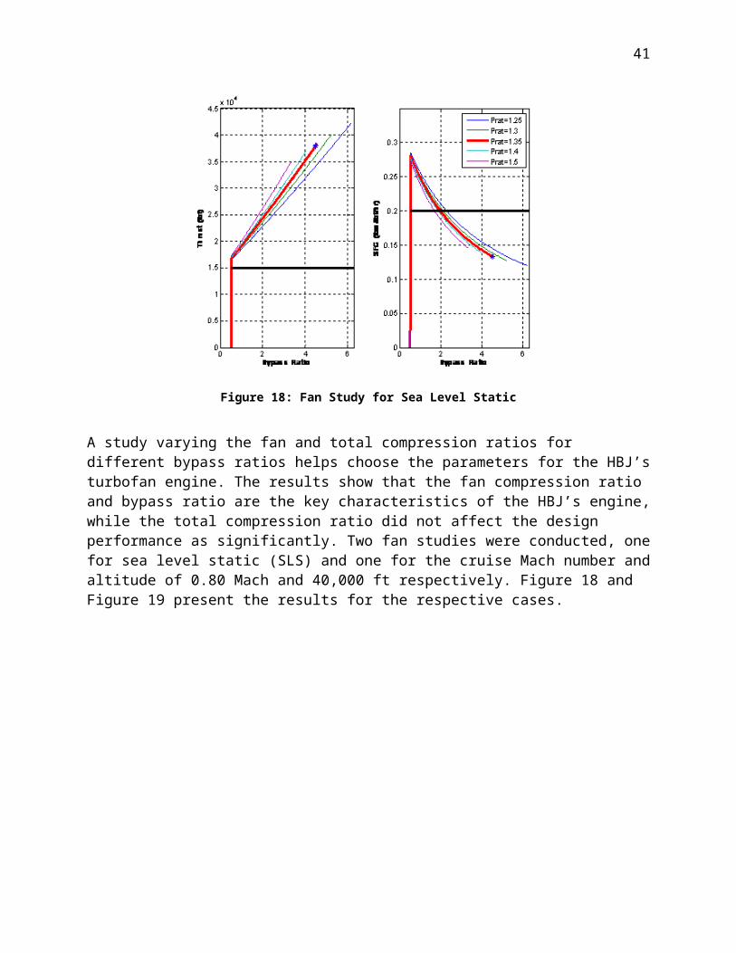
Figure 24: Stability Locations

Equation 7: Yaw Coefficient

Table 31: Federal Aviation Regulations

FAR

Rel

ated

to

Sta

bilit

y

Sec. 25.171 GeneralSec. 25.173 Static longitudinal stabilitySec. 25.175 Demonstration of static

longitudinal stability.Sec. 25.177 Static lateral-directional stabilitySec. 25.181 Dynamic stability

FAR

R

elat

ed to

C

ontro

lSec. 25.143 GeneralSec. 25.145 Longitudinal controlSec. 25.147 Directional and lateral controlSec. 25.149 Minimum control speedSec. 25.161 Trim

FAR

R

elat

ed to

Ta

ke-o

ff

Sec. 25.105 TakeoffSec. 25.107 Takeoff speedsSec. 25.109 Accelerate-stop distanceSec. 25.111 Takeoff pathSec. 25.113 Takeoff distance and takeoff run

FAR

Rel

ated

to

Clim

b

Sec. 25.115 Takeoff flight pathSec. 25.117 Climb: generalSec. 25.119 Landing climb: All-engine-

operatingSec. 25.121 Climb: One-engine-inoperativeSec. 25.123 En route flight paths

Landing Sec. 25.125 Landing

Figure 25: Passenger Cabin Layout

Appendix 5: Carpet Plot Code

% AAE451 PDR Carpet Plotting% AAE451 Spring 2006 Team III:%% Derek Dalton% Megan Darraugh% Sara DaVia% Beau Glim% Seth Hahn% Lauren Nordstrom% Mark Weaver%% This script requires an Excel spreadsheet (here titled carpet_AR_v3.xls)% and reads the data stored within this file in order to generate% individual plots of GTOW, Thrust, Fuel Weight, and L/D against varying% wing loadings. After generating these initial plots from second-order% polynomial curve fits, the intersection points for each individual graph% versus its particular constraint (i.e the three points found from each% GTOW v TW intersecting with the 70,000lb limit on GTOW). After obtaining% these three points, they are plotted and curve-fit to find the% constraining behavior of the given parameter. %% Revised: 15 April 2006

%%%%%%%%%%%%%%%%%%%%%%%%%%%%%%%%%%%%%%%%%%%%%%%%%%%%%%%%%%%%%%%%%%%%%%%%%%%%%% PREPARE WORKSPACE FOR CALCULATION %%%%%%%%%%%%%%%%%%%%%%%%%%%%%%%%%%%%%%%%%%%%%%%%%%%%%%%%%%%%%%%%%%%%%%%%%%%%%%

clc;clear all;close all;

range = 'c3:g15'; % Location in XLS for lowest AR%range = 'c19:g31'; % Location in XLS for middle AR%range = 'c35:g47'; % Location in XLS for highest AR

%%%%%%%%%%%%%%%%%%%%%%%%%%%%%%%%%%%%%%%%%%%%%%%%%%%%%%%%%%%%%%%%%%%%%%%%%%%%%% DEFINE INITIAL VARIABLES %%%%%%%%%%%%%%%%%%%%%%%%%%%%%%%%%%%%%%%%%%%%%%%%%%%%%%%%%%%%%%%%%%%%%%%%%%%%%%

[numbers, text] = xlsread('carpet_AR.xls','v9',range);

w_ss = linspace(20,120,2^11);w_s = [numbers(1,3) numbers(1,4) numbers(1,5)]; % Wing Loading Values

gtow_limit = 70000*ones(size(w_ss));thrust_limit = 15000*ones(size(w_ss));fuel_limit = 11700*ones(size(w_ss));landing_limit = 5600*ones(size(w_ss));

limit = [gtow_limit;thrust_limit;fuel_limit;landing_limit];

%%%%%%%%%%%%%%%%%%%%%%%%%%%%%%%%%%%%%%%%%%%%%%%%%%%%%%%%%%%%%%%%%%%%%%%%%%%%%% FIT INITIAL DATA %%%%%%%%%%%%%%%%%%%%%%%%%%%%%%%%%%%%%%%%%%%%%%%%%%%%%%%%%%%%%%%%%%%%%%%%%%%%%%

k = 1;for n = 2:5 figure(k); hold on; P_35(n-1,:) = POLYFIT(w_s,numbers(n,3:5),2); Y_35(n-1,:) = POLYVAL(P_35(n-1,:),w_ss); plot(w_ss,Y_35(n-1,:),'r-') plot(w_s,numbers(n,3:5),'k*') k = k + 1;

figure(k); hold on; P_45(n-1,:) = POLYFIT(w_s,numbers(n+4,3:5),2); Y_45(n-1,:) = POLYVAL(P_45(n-1,:),w_ss); plot(w_ss,Y_45(n-1,:),'g-') plot(w_s,numbers(n+4,3:5),'k*') k = k + 1; figure(k); hold on; P_55(n-1,:) = POLYFIT(w_s,numbers(n+8,3:5),2); Y_55(n-1,:) = POLYVAL(P_55(n-1,:),w_ss); plot(w_ss,Y_55(n-1,:),'b-') plot(w_s,numbers(n+8,3:5),'k*') k = k + 1;end

%%%%%%%%%%%%%%%%%%%%%%%%%%%%%%%%%%%%%%%%%%%%%%%%%%%%%%%%%%%%%%%%%%%%%%%%%%%%%% DETERMINE CONSTRAINING POINTS %%%%%%%%%%%%%%%%%%%%%%%%%%%%%%%%%%%%%%%%%%%%%%%%%%%%%%%%%%%%%%%%%%%%%%%%%%%%%%

for n = 1:4 q = 1; r = 1; s = 1; for p = 2:length(w_ss) % Start at p=2 because we test p-1 if (Y_35(n,p) < limit(n,1) && Y_35(n,p-1) > limit(n,1)) || ... (Y_35(n,p) > limit(n,1) && Y_35(n,p-1) < limit(n,1)) crit_point_35(n,q) = p; q = q + 1; elseif (Y_45(n,p) < limit(n,1) && Y_45(n,p-1) > limit(n,1)) || ... (Y_45(n,p) > limit(n,1) && Y_45(n,p-1) < limit(n,1)) crit_point_45(n,r) = p; r = r + 1; elseif (Y_55(n,p) < limit(n,1) && Y_55(n,p-1) > limit(n,1)) || ... (Y_55(n,p) > limit(n,1) && Y_55(n,p-1) < limit(n,1)) crit_point_55(n,s) = p; s = s + 1; end endend

%%%%%%%%%%%%%%%%%%%%%%%%%%%%%%%%%%%%%%%%%%%%%%%%%%%%%%%%%%%%%%%%%%%%%%%%%%%%%% PLOT CONSTRAINING POINTS %%%%%%%%%%%%%%%%%%%%%%%%%%%%%%%%%%%%%%%%%%%%%%%%%%%%%%%%%%%%%%%%%%%%%%%%%%%%%%

for n = 1:4 figure(k+n-1); hold on; grid on; plot(w_ss,Y_35(1,:),'r-',w_ss,Y_45(1,:),'g-',w_ss,Y_55(1,:),'b-') legend(strcat(['T/W = ',num2str(numbers(2,1))]), ...

strcat(['T/W = ',num2str(numbers(6,1))]), ... strcat(['T/W = ',num2str(numbers(10,1))]))

% Set the order of the trendline polynomial. if n == 3 order = 2; else order = 1; end

% Plot the trend for varying thrust to weight by selecting the point % where each T/W trendline intersects its corresponding limit % (gtow_limit, thrust_limit, etc) and then plot these points on a % carpet plot of all three T/W vs GTOW curves. Finally, generate and % plot the trendline that best fits these intersection points. cp35 = 1; cp45 = 1; cp55 = 1; if (size(crit_point_35,2) == 2) && (crit_point_35(n,2) ~= 0) cp35 = 2; end if (size(crit_point_45,2) == 2) && (crit_point_45(n,2) ~= 0) cp45 = 2; end if (size(crit_point_55,2) == 2) && (crit_point_55(n,2) ~= 0) cp55 = 2; end plot(w_ss(crit_point_35(n,cp35)),Y_35(1,crit_point_35(n,cp35)),'r*') plot(w_ss(crit_point_45(n,cp45)),Y_45(1,crit_point_45(n,cp45)),'gd') plot(w_ss(crit_point_55(n,cp55)),Y_55(1,crit_point_55(n,cp55)),'bo')

P_C = POLYFIT([w_ss(crit_point_35(n,cp35)), ... w_ss(crit_point_45(n,cp45)), ... w_ss(crit_point_55(n,cp55))], ... [Y_35(1,crit_point_35(n,cp35)), ... Y_45(1,crit_point_45(n,cp45)), ... Y_55(1,crit_point_55(n,cp55))], order);

%set(gca,'xcolor', [0.55 0.55 0.55], 'ycolor', [0.55 0.55 0.55]) set(gca, 'fontsize', 16) xlabel('W/S (lb/ft^2)','color','k', 'fontsize', 16) ylabel('GTOW (lbs)','color','k','fontsize', 16)

Y_C(n,:) = POLYVAL(P_C,w_ss); plot(w_ss,Y_C(n,:),':');end

figure(k+n); hold on; grid on;%set(gca,'xcolor', [0.55 0.55 0.55], 'ycolor', [0.55 0.55 0.55])set(gca,'fontsize',16)plot(w_ss,Y_35(1,:),'r-',w_ss,Y_45(1,:),'g-',w_ss,Y_55(1,:),'b-')plot(w_ss,Y_C(:,:),':');legend(strcat(['T/W = ',num2str(numbers(2,1))]), ...

strcat(['T/W = ',num2str(numbers(6,1))]), ... strcat(['T/W = ',num2str(numbers(10,1))]), ... 'GTOW Limit','Thrust Limit', 'Fuel Limit', 'Landing Limit')xlabel('W/S (lb/ft^2)','color','k','fontsize', 16)ylabel('GTOW (lbs)','color','k','fontsize', 16)

%%%%%%%%%%%%%%%%%%%%%%%%%%%%%%%%%%%%%%%%%%%%%%%%%%%%%%%%%%%%%%%%%%%%%%%%%%%%%% FORMAT FIGURES %%%%%%%%%%%%%%%%%%%%%%%%%%%%%%%%%%%%%%%%%%%%%%%%%%%%%%%%%%%%%%%%%%%%%%%%%%%%%%

for m = 1:k-1 figure(m); grid on %set(gca,'xcolor', [0.55 0.55 0.55], 'ycolor', [0.55 0.55 0.55]) set(gca,'fontsize', 16) if mod(m,3) == 1 tw_text = strcat(['T/W = ',num2str(numbers(2,1))]); elseif mod(m,3) == 2 tw_text = strcat(['T/W = ',num2str(numbers(6,1))]); elseif mod(m,3) == 0 tw_text = strcat(['T/W = ',num2str(numbers(10,1))]); end

if (m >= 1) && (m <= 3) plot(w_ss,gtow_limit,'k:') hash('l',w_ss,gtow_limit,90.25); axis([w_ss(1) w_ss(end) .65*gtow_limit(1) 1.05*gtow_limit(1)])

title(strcat(['W_{TO} vs. Wing Loading for ',tw_text]),'fontsize', 16) xlabel('W/S (lb/ft^2)','color','k','fontsize', 16) ylabel('W_{TO} (lbs)','color','k','fontsize', 16) set(figure(m),'name',strcat([text{1,1},' GTOW/WS for ',tw_text])) elseif (m >= 4) && (m <= 6) plot(w_ss,thrust_limit,'k:') hash('l',w_ss,thrust_limit,91) axis([w_ss(1) w_ss(end) .75*thrust_limit(1) 1.25*thrust_limit(1)])

title(strcat(['Thrust vs. Wing Loading for ',tw_text]),'fontsize', 16) xlabel('W/S (lb/ft^2)','color','k','fontsize', 16) ylabel('Thrust (lbs)','color','k','fontsize', 16) set(figure(m),'name',strcat([text{1,1},' Thrust/WS for ',tw_text])) elseif (m >= 7) && (m <= 9) plot(w_ss,fuel_limit,'k:') hash('l',w_ss,fuel_limit,91) axis([w_ss(1) w_ss(end) .9*fuel_limit(1) 1.4*fuel_limit(1)])

title(strcat(['Fuel Weight vs. Wing Loading for ',tw_text]),'fontsize', 16) xlabel('W/S (lb/ft^2)','color','k','fontsize', 16) ylabel('Fuel Weight (lbs)','color','k','fontsize', 16) set(figure(m),'name',strcat([text{1,1},' Fuel/WS for ',tw_text])) elseif (m >= 10) && (m <= 12) plot(w_ss,landing_limit,'k:') hash('l',w_ss,landing_limit,3) axis([w_ss(1) w_ss(end) .9*landing_limit(1) 1.2*landing_limit(1)])

title(strcat(['Landing Length vs. Wing Loading for ',tw_text]),'fontsize', 16) xlabel('W/S (lb/ft^2)','color','k','fontsize', 16) ylabel('Landing Length (ft)','color','k','fontsize', 16) set(figure(m),'name',strcat([text{1,1},' Landing/WS for ',tw_text])) endend

figure(k) axis([w_ss(1) 60 65000 75000]) title('Constraint Diagram: GTOW','fontsize', 16) set(gcf,'name','Constraint Diagram: GTOW')figure(k+1) axis([w_ss(1) 70 60000 75000]) title('Constraint Diagram: Thrust','fontsize', 16) set(gcf,'name','Constraint Diagram: Thrust')figure(k+2) axis([70 110 55000 65000]) title('Constraint Diagram: Fuel Weight','fontsize', 16) set(gcf,'name','Constraint Diagram: Fuel Weight')figure(k+3) axis([100 110 57500 60000]) title('Constraint Diagram: Landing','fontsize', 16) set(gcf,'name','Constraint Diagram: Landing')figure(k+4) axis([95 w_ss(end) 57500 60000]) title('Overall Constraint Diagram','fontsize', 16) set(gcf,'name','Overall Constraint Diagram') set([1:k+4],'numbertitle','off')

Appendix 6: Engine Design

Density and Temperature Functions

Density as a function of Altitude

y = 0.0006x2 - 0.0669x + 2.3694

y = -0.0276x + 1.69470

0.5

1

1.5

2

2.5

0 10 20 30 40 50

Altitude [kft]

rho

[sl/f

t3*1

0^3]

Figure 26: Density as a Function of Altitude

Temperature as a function of Altitude

y = -3.5602x + 518.66

250

300

350

400

450

500

550

0 10 20 30 40 50

Altitude (kft)

Tem

pera

ture

(R)

Figure 27: Temperature as a Function of Altitude

Flight Envelope Matlab code

% Megan Darraugh% AAE 451% Flight Envelope Code

clcclear all

gam=1.4;R=1716; %[ft-lbf/slug-R]CD=0.025;CLmax=1.8; % !!!!!!!!!!!!!!S=587; %[ft] % !!!!!!!!!!!!!!W_Savg=91.2; % !!!!!!!!!!!!!!n=100;i=0;

for h=linspace(10,59000,n); i=i+1; if h<36000 Temp=-.00356*h + 518.66; rho(i)=(6*10^(-10)*h^2 - 6.69*10^(-5)*h + 2.3694)/1000; else rho(i)=(-.0276/1000*h + 1.6947)/1000; Temp=390; end Mstall(i)=sqrt(2*W_Savg/(rho(i)*CLmax*gam*R*Temp)); M=0.01; error=100000; while error>100 M=M+.001; D=.5*CD*S.*rho(i).*(M*sqrt(gam*R*Temp)).^2; T=62149.6*h^(-.2425)*M^(-.2443); error=abs(T-D); end Drag(i)=D; Thrust(i)=T; Mach(i)=M;endceiling=50000*ones(1,n);Vmax=0.9*ones(1,n);array1=linspace(0,3,n);array2=linspace(0,70000,n);h=linspace(10,60000,n);Vcruise=0.8;hcruise=40000;plot(Mach,h,Mstall,h,'m',array1,ceiling,'g',Vmax,array2,Vcruise,hcruise,'*')legend('Thrust-Drag Limit','Stall Limit','Ceiling','Maximum Speed','Design Point')xlabel('Mach Number')ylabel('Altitude (ft)')axis([0 1.05 0 60000]);

Figure 28: Modified Hydrogen Engines1

Inlet Fan Compression

Total Compression

Combustion Turbine Expansion

Fan Nozzle

Core Flow Nozzle

0.97 0.87 0.85 0.98 0.91 0.93 0.96

Table 32: Assumed Process Efficiencies for Engine Cycle

1 Brand, J. et. Al., Potential Use of Hydrogen in Air Propulsion, AIAA International Air and Space Symposium and Exposition: The Next 100 Years, Ohio, 2003.

3 Miller, Jay, “Air Safety Week,” Project Cryoplane. URL: http://www.findarticles.com/p/articles/mi_m0UBT/is_27_18/ai_n6280702 [cited 21 July 2004].

4 Powers, Laurie, “Flexibly Fueled Storage Tank Brings Hydrogen-Powered Cars Closer To Reality,” Lawrence Livermore National Laboratory, URL: http://www.llnl.gov/str/June03/Aceves.html [cited 25 June 2003].

5 Faab, Reinhard, “Cryoplane,” Airud Deutschland GmbH, URL: http://www.hawhamburg.de/pers/Scholz/dglr/hh/text_2001_12_06_Cryoplane.pdf [cited 6 December 2001].

8 “Future Orbital Transfer Vehicle Technology Study”. NASA Contractor Report 3536. Vol. 2. NASA. 1982

11 Liebeck, R.H., et. Al., “Advanced Subsonic Airplane design and Economic Studies,” NASA CR-195443, 1995.

Engine Cycle Equations

Station ∞ 1 (inlet):

Station 1 2 (fan compression):

Station 2 8 (fan nozzle):

Station 1 3 (compressor):

Station 3 4 (combustor):

**input Tamb, find T04

Table 33: Combustion Calculuation Values

QR hfi H20(g) Cp N2 Cp O2 Cp H2O T0 Air (N2, O2) T0 H2

-240MJ/kmol

-241,827 kJ/kmol

31.98kJ/kmol-K

33.00kJ/kmol-K

40.27kJ/kmol-K Tamb K 298 K

Station 4 5 (high pressure turbine):

**balance of compressor and HP turbine work

Station 5 6 (low pressure turbine):

**balance of fan compressor and LP turbine work

Station 6 7 (core flow nozzle):

Thrust and SFC:

Engine Cycle code

% Megan Darraugh% AAE 451 Spring 2006% Engine code - Hydrogen fueled Turbofan % ----------------------------------------------------------------------% Numbers that were optimized/based off existing engines (and are% therefore subject to change):% 1. all component efficiencies (ni,nf,nc,nt,...)% 2. p02_p01 (fan pressure ratio)% 3. p03_p01 (combined compressor and fan pressure ratio)% 4. beta (bypass ratio- 4 to 8 is high)% 5. A7 & A8 (nozzle exit areas for core flow and bypass flow respectively)% ---------------------------------------------------------------------- % at design point (cruise)Minf=0.8;h=40000; % [ft]pinf=18835; % [kPa] depends on hTinf=216.66; % [K] depends on hgam=1.4; % for pure air (doesn't acct for fuel-air mixt post combustion)R=8314; % inlet (inf-1) --------------------------------------------------------ni=0.97; % typical valueT01=Tinf*(1+(gam-1)/2*Minf^2);T01i=ni*(T01-Tinf)+Tinf;p01=pinf*(T01i/Tinf)^(gam/(gam-1)); % fan (1-2) ------------------------------------------------------------nf=0.87; % typical valuep02_p01=1.35; % (2) optimal value from fan studyT02i=T01*p02_p01^((gam-1)/gam);T02=(T02i-T01)/nf+T01;p02=p02_p01*p01; % fan nozzle (2-8) -----------------------------------------------------njf=0.93; % typical valuep8=pinf; % ----------------------------------T08=T02; % assume Pexit=Pamb then calculateT8i=T02*(p8/p02)^((gam-1)/gam); %T8=T08-njf*(T08-T8i); % Mexit; if Mexit>1 then this assumptionM8=sqrt((T08/T8-1)*2/(gam-1)); %if M8>1 % was wrong, so Mexit=1 then calculate M8=1; % T8=T08*(1+(gam-1)/2*M8^2); % Pexit (same procedure for core nozzle) T8i=T08-(T08-T8)/njf; % P8=p02*(T8i/T02)^(gam/(gam-1)); % ----------------------------------end % compressor (1-3) -----------------------------------------------------nc=0.85; % typical valuep03_p01=25; % (3) optimal value from compressor studyT03i=T01*p03_p01^((gam-1)/gam);

T03=(T03i-T01)/nc+T01;p03=p03_p01*p01; % combustor (3-4) ------------------------------------------------------nb=.98; % typical valuedp=.96; % typical valuep04=dp*p03;T04=(229487+153.22*Tinf)... % adiabatic flame temperature for H2 and air /200.76; % combustion --> T04 DEPENDS ON ALTITUDE because % the entering air temp changesf=0.033; % assumes stoichiometric ratios % high pressure turbine (4-5) ------------------------------------------nt=0.91;T05=(T02-T03)/(1+f)+T04;T05i=T04-(T04-T05)/nt;p05=p04*(T05i/T04)^(gam/(gam-1)); % low pressure turbine (5-6) -------------------------------------------beta=4.5; % (4) optimal value from fan study and compressor studyT06=(T01-T02)*(1+beta)/(1+f)+T05;T06i=T05-(T05-T06)/nt;p06=p05*(T06i/T05)^(gam/(gam-1)); % core nozzle (6-7)-----------------------------------------------------nj=0.96; % typical valuep7=pinf;T07=T06;T7i=T06*(p7/p06)^((gam-1)/gam);T7=T07-nj*(T07-T7i);M7=sqrt((T07/T7-1)*2/(gam-1));if M7>1 M7=1; T7=T07*(1+(gam-1)/2*M7^2); T7i=T07-(T07-T7)/nj; P7=p06*(T7i/T06)^(gam/(gam-1));end % thrust and SFC -------------------------------------------------------A7=0.4; % A=0.4 --> d=0.714mA8=0.7-A7; % A=0.3 --> d=0.944mp07=p7*(1+(gam-1)/2*M7^2)^(gam/(gam-1));T07=T7*(p07/p7)^((gam-1)/gam);D7=DGNonly(M7,gam);mdota=sqrt(gam/R/T07)*p07*A7*D7/(1+f);mdotf=mdota*f;mdotb=mdota*beta;uinf=Minf*sqrt(gam*R*Tinf);u7=M7*sqrt(gam*R*T7);u8=M8*sqrt(gam*R*T8); Thrust_si=mdotb*u8 + (p8-pinf)*A8 + (mdota+mdotf)*u7 + (p7-pinf)*A7 -... (mdota+mdotb)*uinf; % (fan thrust)+(core thrust)-(initial momentum)SFC_si=mdotf/Thrust_si; % [kg/(N*sec)]Thrust=Thrust_si/4.448 % [lbf]SFC=SFC_si*3600*2.205*4.448 % [lbm/(lbf*hr)]

Appendix 7: Configuration Trade Studies

Additional trade studies are done to see if there was a different, optimal, tank configuration for the HBJ. Two trade studies are preformed. Each trade study comprised of redistributing a certain percentage of the fuel volume as well as the tank weight from Tank 1. Trade study 1 redistributed 25% of the fuel to a new location that was aft of the cockpit and forward of the cabin. The remaining 75% of the fuel remanded in Tank 1’s original configuration. Trade study 2 has the same concept but with 33% of the fuel from Tank 1 redistributed to the forward location. Figure 29 shows a graphic visualization of the location for the new CG for each trade study. The blue boxes show trade study 1, the red boxes show trade study 2. The HBJ drawing in Figure 29 is used merely for comparison purposes. In the new configurations for the trade studies the layout of would need to be changed, for example the location of the door and cabin, which can be seen by the location of the windows.

Figure 29: Trade Study Fuel Locations

In trade study 1 there is no significant change in CG from the original configuration. Table 34 shows the CG values for the original configuration as well as for both trade studies. There was, on average, a 1.41ft movement of the CG towards the nose of the aircraft. Trade study 2 showed a larger movement of the CG, moving on average 2.29 ft toward the nose. Granted the average movement was not extremely significant, the individual movement shows a CG movement of 10.79 ft towards the nose in the fully loaded configuration. Again this trade study overall did not show any major advantages over the overall configuration as far as CG is concerned.

Table 34: C.G. Location Trade Study

In trade study 1 and 2 the static margin is significantly better for fueling. So if the HBJ was to be flown with less then full fuel and no passengers or baggage, it would be feasible. Table 35 shows the static margin values for the original configuration as well as for both trade studies. During flight (take-off to decent) the static margin produced in both trade study 1 and 2 are similar in nature in that they are both higher then the original configuration. During take-off and climb the static margins are 20-24% higher then the original configuration. During cruise and decent the static margin is a small percentage higher then the original configuration. Trade study 1 gives the most viable overall static margin of all three configurations in Table 35. Trade study 1 gives positive values for pre flight conditions. Trade study 1 also gives flight values that do not vary as much as the original configuration’s values vary. Also the values are more comparable to comparable aircrafts of the size of the HBJ.

Table 35: Static Margin Trade Study Values

Though numerically trade study 1 seems to be the most optimal configuration, it comes with some negative aspects. Overall when trade study 1 is compared against the hidden cost its downfalls are obvious. Some of the downfalls are the additional production cost of building an additional tank, 5 tanks opposed to 4. Also the forward tank will have to have a small galley way to allow access through the cabin. One of the major, underlying, downfalls of this configuration is the public safety perception that passengers will be sitting between two large hydrogen tanks. Lastly a new structural layout will have to be designed. Once all the variables are taken into consideration, the original configuration was the optimal design.

1 Honeywell, “Honeywell Forecast 2005,” World Aircraft Sales Magazine, URL: http://www.avbuyer.com/PDFs/HoneywellDEC05.pdf [cited 06 February 2006].

2 Westenberger, Andreas, “Cryoplane – Hydrogen Aircraft,” H2 Expo at Hamburg, URL: www.h2hh.de/downloads/Westenberger.pdf [cited 20 April 2006].

6 Airbus Deutschland GmbH, “Liquid Hydrogen Fuelled Aircraft – System Analysis: Final Technical Report,” Competitive and Sustainable Growth’ Programme, URL: http://www.aero-net.org/pdf-docs/20040202-final-technical-report-4-pv.pdf [cited 22 March 2006].

7 Raymer, Dan, Aircraft Design: A Conceptual Approach. AIAA Education Series, New York, New York. 1999.

9 Marchman, Dr. J., “Liberty,” The Virginia Tech Electric General Aviation Team, URL: http://www.aoe.vt.edu/design/vtelectric/Presentation.ppt#293,10,Hydrogen Storage.[cited 15 April 2006]

10 Zydeco, Bill, “All-Composite Cryogenic Tanks,” Microcosm, Inc. Microcosm Space Mission Engineering, URL: http://www.smad.com/scorpius/lowcost/tanks.html [cited 24 April 2006].

12 Guizzo, Erico., “Winner: Carbon takeoff,” IEEE Spectrum, URL: http://www.spectrum.ieee.org/print/2606 [cited 15 April 2006].