viola jones analysis

8/12/2019 Viola Jones Analysis

http://slidepdf.com/reader/full/viola-jones-analysis 1/20

Published in Image Processing On Line on YYYY–MM–DD.

ISSN 2105–1232 c YYYY IPOL & the authors CC–BY–NC–SA

This article is available online with supplementary materials,

software, datasets and online demo at

http://dx.doi.org/10.5201/ipol.YYYY.XXXXXXXX

PREPRINT August 31, 2013

An Analysis of Viola-Jones Face Detection Algorithm

Yi-Qing Wang

CMLA, ENS Cachan, France ([email protected])

Abstract

In this article, we decipher the Viola-Jones algorithm, the first ever real-time face detectionsystem. There are three ingredients working in concert to enable a fast and accurate detection:the integral image for feature computation, Adaboost for feature selection and an attentionalcascade for efficient computational resource allocation. Here we propose a complete algorithmicdescription, a learning code and a learned face detector that can be applied to any color image.Since the Viola-Jones algorithm typically gives multiple detections, a post-processing step isalso proposed to reduce detection redundancy using a robustness argument.

1 Introduction

A face detector has to tell whether an image of arbitrary size contains a human face and if so, whereit is. One natural framework for considering this problem is that of binary classification, in whicha classifier is constructed to minimize the misclassification risk. Since no objective distribution candescribe the actual prior probability for a given image to have a face, the algorithm must minimizeboth the false negative and false positive rates in order to achieve an acceptable performance.

This task requires an accurate numerical description of what sets human faces apart from otherobjects. It turns out that these characteristics can be extracted with a remarkable committee learn-ing algorithm called Adaboost, which relies on a committee of weak classifiers to form a strong onethrough a voting mechanism. A classifier is weak if, in general, it cannot meet a predefined classifi-cation target in error terms.

An operational algorithm must also work with a reasonable computational budget. Techniques suchas integral image and attentional cascade make the Viola-Jones algorithm [10] highly efficient: fedwith a real time image sequence generated from a standard webcam, it performs well on a standardPC.

2 Algorithm

To study the algorithm in detail, we start with the image features for the classification task.

1

http://dx.doi.org/10.5201/ipol

http://creativecommons.org/licenses/by-nc-sa/3.0/



http://creativecommons.org/licenses/by-nc-sa/3.0/

http://dx.doi.org/10.5201/ipol



2.1 Features and integral image

The Viola-Jones algorithm uses Haar-like features, that is, a scalar product between the image andsome Haar-like templates. More precisely, let I and P denote an image and a pattern, both of thesame size N × N (see Figure 1). The feature associated with pattern P of image I is defined by

1≤i≤N

1≤ j≤N

I (i, j)1P (i,j) is white −

1≤i≤N

1≤ j≤N

I (i, j)1P (i,j) is black.

To compensate the effect of different lighting conditions, all the images should be mean and variancenormalized beforehand. Those images with variance lower than one, having little information of interest in the first place, are left out of consideration.

(a) (b) (c)

Figure 1: Haar-like features. Here as well as below, the background of a template like (b) is paintedgray to highlight the pattern’s support. Only those pixels marked in black or white are used whenthe corresponding feature is calculated.

(a) (b) (c) (d) (e)

Figure 2: Five Haar-like patterns. The size and position of a pattern’s support can vary providedits black and white rectangles have the same dimension, border each other and keep their relativepositions. Thanks to this constraint, the number of features one can draw from an image is somewhatmanageable: a 24 × 24 image, for instance, has 43200, 27600, 43200, 27600 and 20736 features of category (a), (b), (c), (d) and (e) respectively, hence 162336 features in all.

In practice, five patterns are considered (see Figure 2 and Algorithm 1). The derived features are

assumed to hold all the information needed to characterize a face. Since faces are by and large regularby nature, the use of Haar-like patterns seems justified. There is, however, another crucial elementwhich lets this set of features take precedence: the integral image which allows to calculate them ata very low computational cost. Instead of summing up all the pixels inside a rectangular window,this technique mirrors the use of cumulative distribution functions. The integral image II of I

II(i, j) :=

1≤s≤i

1≤t≤ j I (s, t), 1 ≤ i ≤ N and 1 ≤ j ≤ N

0, otherwise

is so defined that

N 1≤i≤N 2

N 3≤ j≤N 4

I (i, j) = II(N 2, N 4) − II(N 2, N 3 − 1) − II(N 1 − 1, N 4) + II(N 1 − 1, N 3 − 1) (1)

2



Algorithm 1 Computing a 24 × 24 image’s Haar-like feature vector1: Input: a 24 × 24 image with zero mean and unit variance2: Output: a d × 1 scalar vector with its feature index f ranging from 1 to d3: Set the feature index f ← 04: Compute feature type (a)5: for all (i, j) such that 1 ≤ i ≤ 24 and 1 ≤ j ≤ 24 do

6: for all (w, h) such that i + h − 1 ≤ 24 and j + 2w − 1 ≤ 24 do7: compute the sum S 1 of the pixels in [i, i + h − 1] × [ j, j + w − 1]8: compute the sum S 2 of the pixels in [i, i + h − 1] × [ j + w, j + 2w − 1]9: record this feature parametrized by (1, i , j , w , h): S 1 − S 2

10: f ← f + 111: end for

12: end for

13: Compute feature type (b)14: for all (i, j) such that 1 ≤ i ≤ 24 and 1 ≤ j ≤ 24 do

15: for all (w, h) such that i + h − 1 ≤ 24 and j + 3w − 1 ≤ 24 do

16: compute the sum S 1 of the pixels in [i, i + h − 1] × [ j, j + w − 1]

17: compute the sum S 2 of the pixels in [i, i + h − 1] × [ j + w, j + 2w − 1]18: compute the sum S 3 of the pixels in [i, i + h − 1] × [ j + 2w, j + 3w − 1]19: record this feature parametrized by (2, i , j , w , h): S 1 − S 2 + S 320: f ← f + 121: end for

22: end for

23: Compute feature type (c)24: for all (i, j) such that 1 ≤ i ≤ 24 and 1 ≤ j ≤ 24 do

25: for all (w, h) such that i + 2h − 1 ≤ 24 and j + w − 1 ≤ 24 do

26: compute the sum S 1 of the pixels in [i, i + h − 1] × [ j, j + w − 1]27: compute the sum S 2 of the pixels in [i + h, i + 2h − 1] × [ j, j + w − 1]28: record this feature parametrized by (3, i , j , w , h): S 1 − S 2

29: f ← f + 130: end for

31: end for

32: Compute feature type (d)33: for all (i, j) such that 1 ≤ i ≤ 24 and 1 ≤ j ≤ 24 do

34: for all (w, h) such that i + 3h − 1 ≤ 24 and j + w − 1 ≤ 24 do

35: compute the sum S 1 of the pixels in [i, i + h − 1] × [ j, j + w − 1]36: compute the sum S 2 of the pixels in [i + h, i + 2h − 1] × [ j, j + w − 1]37: compute the sum S 3 of the pixels in [i + 2h, i + 3h − 1] × [ j, j + w − 1]38: record this feature parametrized by (4, i , j , w , h): S 1 − S 2 + S 339: f ← f + 140: end for

41: end for42: Compute feature type (e)43: for all (i, j) such that 1 ≤ i ≤ 24 and 1 ≤ j ≤ 24 do

44: for all (w, h) such that i + 2h − 1 ≤ 24 and j + 2w − 1 ≤ 24 do

45: compute the sum S 1 of the pixels in [i, i + h − 1] × [ j, j + w − 1]46: compute the sum S 2 of the pixels in [i + h, i + 2h − 1] × [ j, j + w − 1]47: compute the sum S 3 of the pixels in [i, i + h − 1] × [ j + w, j + 2w − 1]48: compute the sum S 4 of the pixels in [i + h, i + 2h − 1] × [ j + w, j + 2w − 1]49: record this feature parametrized by (5, i , j , w , h): S 1 − S 2 − S 3 + S 450: f ← f + 151: end for

52: end for

3



holds for all N 1 ≤ N 2 and N 3 ≤ N 4. As a result, computing an image’s rectangular local sum requiresat most four elementary operations given its integral image. Moreover, obtaining the integral imageitself can be done in linear time: setting N 1 = N 2 and N 3 = N 4 in (1), we find

I (N 1, N 3) = II(N 1, N 3) − II(N 1, N 3 − 1) − II(N 1 − 1, N 3) + II(N 1 − 1, N 3 − 1).

Hence a recursive relation which leads to Algorithm 3.

As a side note, let us mention that once the useful features have been selected by the boostingalgorithm, one needs to scale them up accordingly when dealing with a bigger window (see Algorithm2). Smaller windows, however, will not be looked at.

2.2 Feature selection with Adaboost

How to make sense of these features is the focus of Adaboost [1].

Some terminology. A classifier maps an observation to a label valued in a finite set. For face detection,it assumes the form of f : Rd → {−1, 1}, where 1 means that there is a face and −1 the contrary

and d is the number of Haar-like features extracted from an image. Given the probabilistic weightsw· ∈ R+ assigned to a training set made up of n observation-label pairs (xi, yi), Adaboost aims toiteratively drive down an upper bound of the empirical loss

ni=1

wi1yi=f (xi)

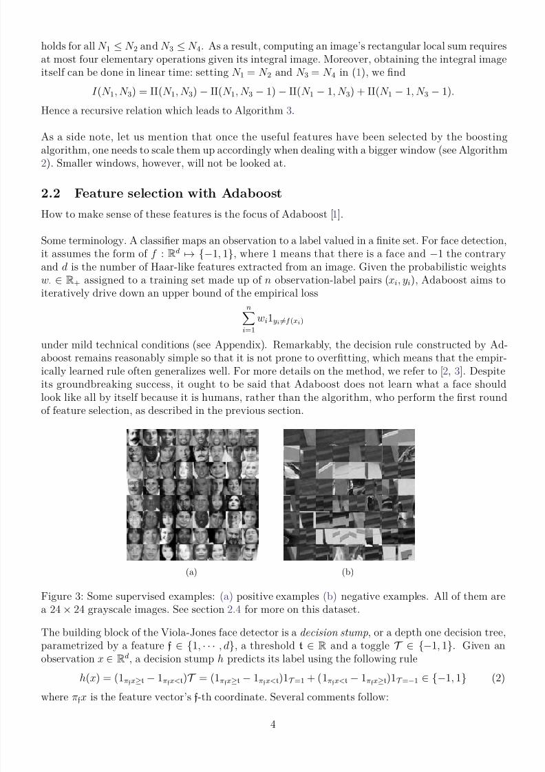
under mild technical conditions (see Appendix). Remarkably, the decision rule constructed by Ad-aboost remains reasonably simple so that it is not prone to overfitting, which means that the empir-ically learned rule often generalizes well. For more details on the method, we refer to [ 2, 3]. Despiteits groundbreaking success, it ought to be said that Adaboost does not learn what a face shouldlook like all by itself because it is humans, rather than the algorithm, who perform the first roundof feature selection, as described in the previous section.

(a) (b)

Figure 3: Some supervised examples: (a) positive examples (b) negative examples. All of them area 24 × 24 grayscale images. See section 2.4 for more on this dataset.

The building block of the Viola-Jones face detector is a decision stump, or a depth one decision tree,parametrized by a feature f ∈ {1, · · · , d}, a threshold t ∈ R and a toggle T ∈ {−1, 1}. Given anobservation x ∈ Rd, a decision stump h predicts its label using the following rule

h(x) = (1πfx≥t − 1πfx<t )T = (1πfx≥t − 1πfx<t )1T =1 + (1πfx<t − 1πfx≥t )1T =−1 ∈ {−1, 1} (2)

where πfx is the feature vector’s f-th coordinate. Several comments follow:

4



Algorithm 3 Integral Image1: Input: an image I of size N × M .2: Output: its integral image II of the same size.3: Set II(1, 1) = I (1, 1).4: for i = 1 to N do

5: for j = 1 to M do

6: II(i, j) = I (i, j) + II(i, j − 1) + II(i − 1, j) − II(i − 1, j − 1) and II is defined to be zero whenever itsargument (i, j) ventures out of I ’s domain.

7: end for

8: end for

1. any additional pattern produced by permuting black and white rectangles in an existing pattern(see Figure 2) is superfluous. Because such a feature is merely the opposite of an existingfeature, only a sign change for t and T is needed to have the same classification rule.

2. if the training examples are in ascending order of a given feature f, a linear time exhaustivesearch on the threshold and toggle can find a decision stump using this feature that attains thelowest empirical loss

ni=1

wi1yi=h(xi) (3)

on the training set (see Algorithm 4). Imagine a threshold placed somewhere on the real line,if the toggle is set to 1, the resulting rule will declare an example x positive if πfx is greaterthan the threshold and negative otherwise. This allows us to evaluate the rule’s empirical error,thereby selecting the toggle that fits the dataset better (lines 8–16 of Algorithm 4).

Since margin

mini: yi=−1

|πfxi − t | + mini: yi=1

|πfxi − t |

and risk, or the expectation of the empirical loss (3), are closely related [3, 6, 7], of two decisionstumps having the same empirical risk, the one with a larger margin is preferred (line 14 of Algorithm 4). Thus in absence of duplicates, there are n+1 possible thresholds and the one withthe smallest empirical loss should be chosen. However it is possible to have the same featurevalues from different examples and extra care must be taken to handle this case properly (lines27–32 of Algorithm 4).

By adjusting individual example weights (Algorithm 6 line 10), Adaboost makes more effort to learn

harder examples and adds more decision stumps in the process. Intuitively, in the final voting, astump ht with lower empirical loss is rewarded with a bigger say (a higher αt, see Algorithm 6 line9) when a T -member committee (vote-based classifier) assigns an example according to

f T (·) = sign T

t=1

αtht(·).

How the training examples should be weighed is explained in detail in Appendix. Figure 4 shows aninstance where Adaboost reduces false positive and false negative rates simultaneously as more andmore stumps are added to the committee. For notational simplicity, we denote the empirical loss by

ni=1

wi(1)1yiT

t=1 αtht(xi)≤0

:= P(f T (X ) = Y )

6



Algorithm 4 Decision Stump by Exhaustive Search1: Input: n training examples arranged in ascending order of feature πfxi: πfxi1 ≤ πfxi2 ≤ · · · ≤ πfxin ,

probabilistic example weights (wk)1≤k≤n.2: Output: the decision stump’s threshold τ , toggle T , error E and margin M.3: Initialization: τ ← min1≤i≤n πfxi − 1, M ← 0 and E ← 2 (an arbitrary upper bound of the empirical

loss).4: Sum up the weights of the positive (resp. negative) examples whose f-th feature is bigger than the present

threshold: W +

1 ←

n

i=1wi1y

i=1 (resp. W +

−1 ←

n

i=1wi1y

i=−1).

5: Sum up the weights of the positive (resp. negative) examples whose f-th feature is smaller than thepresent threshold: W −1 ← 0 (resp. W −−1 ← 0).

6: Set iterator j ← 0, τ ← τ and M ← M.7: while true do

8: Select the toggle to minimize the weighted error : error+ ← W −1 + W +−1 and error− ← W +1 + W −−1.9: if error+ < error− then

10: E ← error+ and T ← 1.11: else

12: E ← error− and T ← −1.13: end if

14: if

E < E or

E = E &

M > M then

15: E ← E , τ ← τ , M ← M and T ← T .16: end if

17: if j = n then

18: Break.19: end if

20: j ← j + 1.21: while true do

22: if yij = −1 then

23: W −−1 ← W −−1 + wij and W +−1 ← W +−1 − wij .24: else

25: W −1 ← W −1 + wij and W +1 ← W +1 − wij .26: end if

27: To find a new valid threshold, we need to handle duplicate features.

28: if j = n or πfxij = πfxij+1 then

29: Break.30: else

31: j ← j + 1.32: end if

33: end while

34: if j = n then

35: τ ← max1≤i≤n πfxi + 1 and M ← 0.36: else

37:

τ ← (πfxij + πfxij+1)/2 and

M ← πfxij+1 − πfxij .

38: end if 39: end while

Algorithm 5 Best Stump1: Input: n training examples, their probabilistic weights (wi)1≤i≤n, number of features d.2: Output: the best decision stump’s threshold, toggle, error and margin.3: Set the best decision stump’s error to 2.4: for f = 1 to d do

5: Compute the decision stump associated with feature f using Algorithm 4.6: if this decision stump has a lower weighted error (3) than the best stump or a wider margin if the

weighted error are the same then

7: set this decision stump to be the best.8: end if

9: end for

7



(a) (b)

Figure 4: Algorithm 6 ran with equally weighted 2500 positive and 2500 negative examples. Figure(a) shows that the empirical risk and its upper bound, interpreted as the exponential loss (seeAppendix), decrease steadily over iterations. This implies that false positive and false negative ratesmust also decrease, as observed in (b).

zero. However, our own experience tells us that in an image, a rather limited number of sub-windowsdeserve more attention than others. This is true even for face-intensive group photos. Hence theidea of a multi-layer attentional cascade which embodies a principle akin to that of Shannon coding:the algorithm should deploy more resources to work on those windows more likely to contain a facewhile spending as little effort as possible on the rest.

Each layer in the attentional cascade is expected to meet a training target expressed in false positiveand false negative rates: among n negative examples declared positive by all of its preceding layers,layer l ought to recognize at least (1 − αl)n as negative and meanwhile try not to sacrifice its perfor-mance on the positives: the detection rate should be maintained above 1 − β l.

At the end of the day, only the generalization error counts which unfortunately can only be estimatedwith some validation examples that Adaboost is not allowed to see at the training phase. Hence inAlgorithm 10 at line 10, a conservative choice is made as to how one assesses the error rates: thehigher false positive rate obtained from training and validation is used to evaluate how well thealgorithm has learned to distinguish faces from non-faces. The false negative rate is assessed in thesame way.

It should be kept in mind that Adaboost by itself does not favor either error rate: it aims to reduceboth simultaneously rather than one at the expense of the other. To allow flexibility, one additionalcontrol s ∈ [−1, 1] is introduced to shift the classifier

f T s (·) = sign

T t=1

αt

ht(·) + s

(4)

so that a strictly positive s makes the classifier more inclined to predict a face and vice versa.

To enforce an efficient resource allocation, the committee size should be small in the first few layersand then grow gradually so that a large number of easy negative patterns can be eliminated with

9



little computational effort (see Figure 5).

Algorithm 7 Detecting faces with an Adaboost trained cascade classifier1: Input: an M × N grayscale image I and an L-layer cascade of shifted classifiers trained using Algorithm

102: Parameter: a window scale multiplier c

3: Output: P , the set of windows declared positive by the cascade4: Set P = {[i, i + e − 1] × [ j, j + e − 1] ⊂ I : e = 24cκ, κ ∈ N}

5: for l = 1 to L do

6: for every window in P do

7: Remove the windowed image’s mean and compute its standard deviation.8: if the standard deviation is bigger than 1 then

9: divide the image by this standard deviation and compute its features required by the shiftedclassifier at layer l with Algorithm 2

10: if the cascade’s l-th layer predicts negative then

11: discard this window from P 12: end if

13: else

14: discard this window from P 15: end if

16: end for

17: end for

18: Return P

Appending a layer to the cascade means that the algorithm has learned to reject a few new negativepatterns previously viewed as difficult, all the while keeping more or less the same positive trainingpool. To build the next layer, more negative examples are thus required to make the training processmeaningful. To replace the detected negatives, we run the cascade on a large set of gray images withno human face and collect their false positive windows. The same procedure is used for constructingand replenishing the validation set (see Algorithm 7). Since only 24 × 24 sized examples can be usedin the training phase, those bigger false positives are recycled using Algorithm 9.

Algorithm 8 Downsampling a square image1: Input: an e × e image I (e > 24)2: Output: a downsampled image O of dimension 24 × 24

3: Blur I using a Gaussian kernel with standard deviation σ = 0.6

( e24 )2 − 1

4: Allocate a matrix O of dimension 24 × 245: for i = 0 to 23 do

6: for j = 0 to 23 do

7: Compute the scaled coordinates ˜i ←

e−1

25 (i + 1), ˜ j ←

e−1

25 ( j + 1)8: Set imax ← min(i + 1, e − 1), imin ← max(0, i), jmax ← min(˜ j + 1, e − 1), jmin ← max(0, ˜ j)9: Set O(i, j) = 1

4

I (imax, ˜ jmax) + I (imin, ˜ jmax) + I (imin, ˜ jmin) + I (imax, ˜ jmin)

10: end for

11: end for

12: Return O

Assume that at layer l, a committee of T l weak classifiers is formed along with a shift s so that theclassifier’s performance on training and validation set can be measured. Let us denote the achievedfalse positive and false negative rate by αl and β l. Depending on their relation with the targets αl

and β l, four cases are presented:

1. if the layer training target is fulfilled (Algorithm 10 line 11: αl ≤ αl and β l ≤ β l), the algorithmmoves on to training the next layer if necessary.

10



Algorithm 10 Attentional Cascade1: Input: n training positives, m validation positives, two sets of gray images with no human faces to draw

training and validation negatives, desired overall false positive rate αo, and targeted layer false positiveand detection rate αl and 1 − β l.

2: Parameter: maximum committee size at layer l: N l = min(10l + 10, 200).3: Output: a cascade of committees.4: Set the attained overall false positive rate

αo ← 1 and layer count l ← 0.

5: Randomly draw 10n negative training examples and m negative validation examples.6: while αo > αo do

7: u ← 10−2, l ← l + 1, sl ← 0, and T l ← 1.8: Run Algorithm 6 on the training set to produce a classifier f T l

l = signT l

t=1 αtht

.

9: Run the sl-shifted classifier

f T ll,sl

= sign T l

t=1

αt

ht + sl

on both the training and validation set to obtain the empirical and generalized false positive (resp.false negative) rate αe and αg (resp. β e and β g).

10:

αl ← max(αe, αg) and

β l ← max(β e, β g).

11: if αl ≤ αl and 1 − β l ≥ 1 − β l then

12: αo ← αo × αl.13: else if αl ≤ αl, 1 − β l < 1 − β l and u > 10−5 (there is room to improve the detection rate) then

14: sl ← sl + u.15: if the trajectory of sl is not monotone then

16: u ← u/2.17: sl ← sl − u.18: end if

19: Go to line 9.20: else if αl > αl, 1 − β l ≥ 1 − β l and u > 10−5 (there is room to improve the false positive rate) then

21: sl ← sl − u.

22: if the trajectory of sl is not monotone then23: u ← u/2.24: sl ← sl + u.25: end if

26: Go to line 9.27: else

28: if T l > N l then

29: sl ← −130: while 1 − β l < 0.99 do

31: Run line 9 and 10.32: end while

33:

αo ←

αo ×

αl.

34: else35: T l ← T l + 1 (Train one more member to add to the committee.)36: Go to line 8.37: end if

38: end if

39: Remove the false negatives and true negatives detected by the current cascade

f cascade(X ) = 2 l p=1

1f T pp,sp

(X )=1 −

1

2

.

Use this cascade with Algorithm 9 to draw some false negatives so that there are n training negatives

and m validation negatives for the next round.40: end while

41: Return the cascade.

12



A window is thus declared positive if and only if all its component layers hold the same opinion

P(f cascade(X ) = 1|Y = −1)

=P(L

l=1

{f T ll, sl

(X ) = 1}|Y = −1)

=P(f T LL, sL

(X ) = 1|L−1

l=1

{f T ll, sl

(X ) = 1} and Y = −1)P(L−1

l=1

{f T ll, sl

(X ) = 1}|Y = −1)

≤αlP(L−1l=1

{f T ll, sl

(X ) = 1}|Y = −1)

≤αLl .

Likewise, the overall detection rate can be estimated as follows

P(f cascade(X ) = 1|Y = 1)

=P(L

l=1

{f T ll, sl

(X ) = 1}|Y = 1)

=P(f T LL, sL

(X ) = 1|L−1l=1

{f T ll, sl

(X ) = 1} and Y = 1)P(L−1l=1

{f T ll, sl

(X ) = 1}|Y = 1)

≥(1 − β l)P(L−1l=1

{f T ll, sl

(X ) = 1}|Y = 1)

≥(1 − β l)L.

In other words, if the empirically obtained rates are any indication, a faceless window will have aprobability higher than 1−αl to be labeled as such at each layer, which effectively directs the cascadeclassifier’s attention on those more likely to have a face (see Figure 6).

2.4 Dataset and Experiments

A few words on the actual cascade training carried out on a 8-core Linux machine with 48G memory.We first downloaded 2897 different images without human faces from [4, 9, 5], National Oceanic andAtmospheric Administration (NOAA) Photo Library1 and European Southern Observatory2. Theywere divided into two sets containing 2451 and 446 images respectively for training and validation.1000 training and 1000 validation positive examples from an online source3 were used. The trainingprocess lasted for around 24 hours before producing a 31-layer cascade. It took this long because itbecame harder to get 2000 false positives (1000 for training and 1000 for validation) using Algorithm9 with a more discriminative cascade: the algorithm needed to examine more images before it could

come across enough good examples. The targeted false positive and false negative rate for each layerwere set to 0.5 and 0.995 respectively and Figure 7 shows how the accumulated false positive rate asdefined at line 12 and 33 of Algorithm 10 evolves together with the committee size. The fact thatthe later layers required more intensive training also contributed to a long training phase.

3 Post-Processing

Figure 6(d) and Figure 8(a) show that the same face can be detected multiple times by a correctlytrained cascade. This should come as no surprise as the positive examples (see Figure 3(a)) do allow

1

http://www.photolib.noaa.gov/2http://www.eso.org/public/images/3http://www.cs.wustl.edu/ pless/559/Projects/faceProject.html

13

http://www.photolib.noaa.gov/


http://www.eso.org/public/images/

http://www.cs.wustl.edu/~pless/559/Projects/faceProject.html















(a) (b) (c) (d) (e) (f)

(g) (h) (i) (j) (k) (l)

(m) (n) (o) (p) (q) (r)

(s) (t) (u) (v) (w) (x)

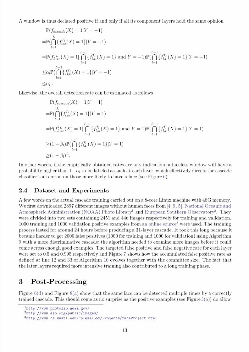
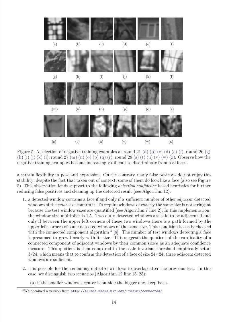
Figure 5: A selection of negative training examples at round 21 (a) (b) (c) (d) (e) (f), round 26 (g)(h) (i) (j) (k) (l), round 27 (m) (n) (o) (p) (q) (r), round 28 (s) (t) (u) (v) (w) (x). Observe how thenegative training examples become increasingly difficult to discriminate from real faces.

a certain flexibility in pose and expression. On the contrary, many false positives do not enjoy thisstability, despite the fact that taken out of context, some of them do look like a face (also see Figure5). This observation lends support to the following detection confidence based heuristics for furtherreducing false positives and cleaning up the detected result (see Algorithm 12):

1. a detected window contains a face if and only if a sufficient number of other adjacent detectedwindows of the same size confirm it. To require windows of exactly the same size is not stringentbecause the test window sizes are quantified (see Algorithm 7 line 2). In this implementation,the window size multiplier is 1.5. Two e × e detected windows are said to be adjacent if andonly if between the upper left corners of these two windows there is a path formed by the

upper left corners of some detected windows of the same size. This condition is easily checkedwith the connected component algorithm 4 [8]. The number of test windows detecting a faceis presumed to grow linearly with its size. This suggests the quotient of the cardinality of aconnected component of adjacent windows by their common size e as an adequate confidencemeasure. This quotient is then compared to the scale invariant threshold empirically set at3/24, which means that to confirm the detection of a face of size 24 ×24, three adjacent detectedwindows are sufficient.

2. it is possible for the remaining detected windows to overlap after the previous test. In thiscase, we distinguish two scenarios (Algorithm 12 line 15–25):

(a) if the smaller window’s center is outside the bigger one, keep both.4We obtained a version from http://alumni.media.mit.edu/˜rahimi/connected/.

14

http://alumni.media.mit.edu/~rahimi/connected/






(a) (b)

(c) (d)

Figure 6: How the trained cascade performs with (a) 16 layers, (b) 21 layers, (c) 26 layers and (d)31 layers: the more layers, the less false positives.

(b) keep the one with higher detection confidence otherwise.

Finally, to make the detector slightly more rotation-invariant, in this implementation, we decided torun Algorithm 7 three times, once on the input image, once on a clockwise rotated image and onceon an anti-clockwise rotated image before post-processing all the detected windows (see Algorithm

13). In addition, when available, color also conveys valuable information to help further eliminatefalse positives as explained in [11]. Hence in the current implementation, after the robustness test,an option is offered as to whether color images should be post-processed with this additional step(see Algorithm 11). If so, a detected window is declared positive only if it passes both tests.

15



Algorithm 11 Skin Test1: Input: an N × N color image I 2: Output: return whether I has enough skin like pixels3: Set a counter c ← 0

4: for each pixel in I do5: if the intensities of its green and blue channel are lower than that of its red channel then

6: c ← c + 17: end if

8: end for

9: if c/N 2 > 0.4 then

10: Return true11: else

12: Return false13: end if

Algorithm 12 Post-Processing1: Input: a set G windows declared positive on an M × N grayscale image2: Parameter: minimum detection confidence threshold r

3: Output: a reduced set of positive windows P 4: Create an M × N matrix E filled with zeros.

5: for each window w ∈ G do6: Take w ’s upper left corner coordinates (i, j) and its size e and set E (i, j) ← e7: end for

8: Run a connected component algorithm on E .9: for each component C formed by |C | detected windows of dimension eC × eC do

10: if its detection confidence |C |e−1C > r then

11: send one representing window to P 12: end if

13: end for

14: Sort the elements in P in ascending order of window size.15: for window i = 1 to |P | do

16: for window j = i + 1 to |P | do

17: if window j remains in P and the center of window i is inside of window j then

18: if window i has a higher detection confidence than window j then

19: remove window j from P 20: else

21: remove window i from P and break from the inner loop22: end if

23: end if

24: end for

25: end for

26: Return P .

16



(a) (b)

Figure 7: (a) Though occasionally stagnant, the accumulated false positive rate declines pretty fastwith the number of layers. (b) As the learning task becomes more difficult as the cascade has morelayers, more weak learners per layer are called upon. (In our experiments, the number of weaklearners cannot exceed 201 per layer.)

Algorithm 13 Face detection with image rotation1: Input: an M × N grayscale image I 2: Parameter: rotation θ3: Output: a set of detected windows P 4: Rotate the image about its center by θ and −θ to have I θ and I −θ

5: Run Algorithm 7 on I , I θ and I −θ to obtain three detected window sets P , P θ and P −θ respectively6: for each detected window w in P θ do

7: Get w ’s upper left corner’s coordinates (iw, jw) and its size ew

8: Rotate (iw, jw) about I θ’s center by −θ to get (iw, ˜ jw)9: Quantify the new coordinates iw ← min(max(0, iw), M − 1) and jw ← min(max(0, ˜ jw), N − 1)

10: if there is no ew × ew window located at (˜iw,

˜ jw) in P then11: Add it to P

12: end if

13: end for

14: Replace θ by −θ and go through lines 6–13 again15: Return P

4 Appendix

This section explains, from a mathematical perspective, how and why Adaboost (Algorithm 6) works.We define the exponential loss

∀(x, y) ∈ Rd × {−1, 1}, L(y, f (x)) = exp(−yf (x))

where the classifier f : Rd → R takes the form of a linear combination of weak classifiers

f (·) =T

t=1

αtht(·)

with T ∈ N, min1≤t≤T αt > 0 and ∀t, ht(·) ∈ {−1, 1}. Naturally, the overall objective is

minht,αt≥0

ni=1

wi(1)L(yi,T

t=1

αtht(xi)) (5)

with some initial probabilistic weight wi(1). A greedy approach is deployed to deduce the optimalclassifiers ht and weights αt one after another, although there is no guarantee that the objective (5)

17



(a)

(b)

Figure 8: The suggested post-processing procedure further eliminates a number of false positives andbeautifies the detected result using a 31 layer cascade. Image credit: Google

is minimized. Given (αs, hs)1≤s<t, let Z t+1 be the weighted exponential loss attained by a t-member

18



committee and we seek to minimize it through (ht, αt)

Z t+1 := minht,αt≥0

ni=1

wi(1)e−yit

s=1 αshs(xi)

= minht,αt≥0

ni=1

Di(t)e−αtyiht(xi)

= minht,αt≥0

n

i=1

Di(t)e−αt1yiht(xi)=1 +n

i=1

Di(t)eαt1yiht(xi)=−1

= minht,αt≥0

e−αt

ni=1

Di(t) + (eαt − e−αt)n

i=1

Di(t)1yiht(xi)=−1

=Z t minht,αt≥0

e−αt + (eαt − e−αt)n

i=1

Di(t)

Z t1yiht(xi)=−1

with for all t > 1

Di(t) := wi(1)e−yit−1

s=1 αshs(xi), ∀i ∈ {1, · · · , n} with Z t =

n

i=1

Di(t).

Therefore the optimisation of Z t+1 can be carried out in two stages: first, because of αt’s assumedpositivity, we minimize the weighted error using a base learning algorithm, a decision stump forinstance

ǫt := minh

Z −1t

ni=1

Di(t)1yih(xi)=−1

ht := argminh

Z −1t

ni=1

Di(t)1yih(xi)=−1.

In case of multiple minimizers, take ht to be any of them. Next choose

αt = 1

2 ln

1 − ǫt

ǫt

= argminα>0

e−α + (eα − e−α)ǫt.

Hence ǫt < 0.5 is necessary, which imposes a minimal condition on the training set and the baselearning algorithm. Also obtained is

Z t+1 = 2Z t

ǫt(1 − ǫt) ≤ Z t

a recursive relation asserting the decreasing behavior of the exponential risk. Weight change thus

depends on whether an observation is misclassified

wi(t + 1) = Di(t + 1)

Z t+1=

Di(t)e−yiαtht(xi)

2Z t

ǫt(1 − ǫt)=

wi(t)

2

1ht(xi)=yi

1

1 − ǫt

+ 1ht(xi)=yi

1

ǫt

.

The final boosted classifier is thus a weighted committee

f (·) := sign T

t=1

αtht(·).

19



References

[1] Y. Freund and R. Schapire. A decision-theoretic generalization of on-line learning and anapplication to boosting. Journal of Computer and System Sciences , 55(1):119–139, 1997.http://dx.doi.org/10.1006/jcss.1997.1504.

[2] Y. Freund, R. Schapire, and N. Abe. A short introduction to boosting. Journal of Japanese

Society For Artificial Intelligence , 14(771-780):1612, 1999.

[3] J. Friedman, T. Hastie, and R. Tibshirani. The Elements of Statistical Learning , volume 1.Springer Series in Statistics, 2001.

[4] H. Jegou, M. Douze, and C. Schmid. Hamming embedding and weak geometric consistencyfor large scale image search. In European Conference on Computer Vision , volume I of Lecture

Notes in Computer Science , pages 304–317. Springer, 2008.

[5] A. Olmos. A biologically inspired algorithm for the recovery of shading and reflectance images.Perception , 33(12):1463, 2004. http://dx.doi.org/10.1068/p5321.

[6] F. Rosenblatt. The perceptron: a probabilistic model for information storage and organizationin the brain. Psychological review , 65(6):386, 1958. http://dx.doi.org/10.1037/h0042519.

[7] R. E. Schapire, Y. Freund, P. Bartlett, and W. S. Lee. Boosting the margin: A new explanationfor the effectiveness of voting methods. The Annals of Statistics , 26(5):1651–1686, 1998. http://dx.doi.org/10.1214/aos/1024691352.

[8] L. Shapiro and G.C. Stockman. Computer vision, 2001.

[9] G. Tkacik, P. Garrigan, C. Ratliff, G. Milcinski, J. M. Klein, L. H. Seyfarth, P. Sterling, D. H.Brainard, and V. Balasubramanian. Natural images from the birthplace of the human eye.

Public Library of Science One , 6(6):e20409, 2011.

[10] P. Viola and M. J. Jones. Robust real-time face detection. International Journal of Computer

Vision , 57(2):137–154, 2004. http://dx.doi.org/10.1023/B:VISI.0000013087.49260.fb.

[11] S. Wang and A. Abdel-Dayem. Improved viola-jones face detector. In Taibah University Inter-

national Conference on Computing and Information Technology , pages 123–128, 2012.

20

http://dx.doi.org/10.1006/jcss.1997.1504

http://dx.doi.org/10.1068/p5321

http://dx.doi.org/10.1037/h0042519

http://dx.doi.org/10.1037/h0042519

http://dx.doi.org/10.1214/aos/1024691352


http://dx.doi.org/10.1023/B:VISI.0000013087.49260.fb





http://dx.doi.org/10.1037/h0042519

http://dx.doi.org/10.1068/p5321

http://dx.doi.org/10.1006/jcss.1997.1504

viola jones analysis

Documents