virginia c. vera and don c. lawton - crewes.org · virginia c. vera and don c. lawton abstract...

Fluid substitution sandstone aquifer

CREWES Research Report — Volume 22 (2010) 1

Fluid substitution and seismic modelling in a sandstone aquifer

Virginia C. Vera and Don C. Lawton

ABSTRACT

Fluid substitution and seismic modelling were applied in order to evaluate the Paskapoo Formation as a potential CO2 geological storage unit. The first stage of this project deals with the application of the Gassmann substitution model using well data and evaluation of property variations due to CO2 saturation changes. Seismic modelling was undertaken in the area of interest simulating pre, during and post CO2 injection scenarios. From Gassmann calculations it was found that the P-wave velocity drops between 0 to 20% CO2 saturation and starts a subtle rise at 30% whereas the S-wave velocity increases directly proportional to CO2 saturation. The P-wave velocity decreases approximately 7%, the S-wave velocity increases 0.8 %, Vp/Vs decreases an average value of 8% and the basal reflector presents a time delay of 1.6 msec. From seismic modelling it was found that the injection zone can be delineated in the CDP stack section through an amplitude change the top reflector and a time delay for the basal reflector. The reflectivity coefficient was evaluated using the Shuey approximation and qualitative observations of the sections, showing a decrease in the reflectivity with increasing CO2 saturation, with a major drop in the first 10% and a further amplitude decrease with offset (higher angles). These parameters allow us to estimate the conditions that would help to interpret the real data in further phases of this study.

INTRODUCTION

The inevitable and fast increase of the greenhouse gases concentrations and hypnotized global warming, constitute one of society’s major concerns presently. The excess of CO2 in the atmosphere is considered by many to be the principal cause of the problem, affecting the natural equilibrium. CO2 sequestration in geological sites represents a viable solution or at least a way of mitigation. The idea of this method is to capture CO2 produced by anthropogenic or natural point sources and inject it into a porous layer surrounded by non porous layers to trap the gas (Hovorka, 2008).

The main objective of this project is to evaluate Paskapoo Formation as a potential test CO2 geological storage site. A fluid substitution model was performed using well information to estimate the effects and changes due to CO2 injection. Synthetic seismograms were generated for each CO2 saturation value. Gassmann equations were applied in order to evaluate changes in the P-wave and the S-wave velocity. Finally a 2D seismic model of the area was created with the respective density and velocity parameters obtained from well information. The zone of injection is defined inside the model. Six (6) CDP stack sections were created: 0%, 20%, 40%, 60%, 80% and 100% CO2 saturation, changing parameters for each saturation stage. This model provides some ideas about the seismic respond depending on the CO2 saturation and the evolution of the injection process.

Vera and Lawton

2 CREWES Research Report — Volume 22 (2010)

AREA OF STUDY

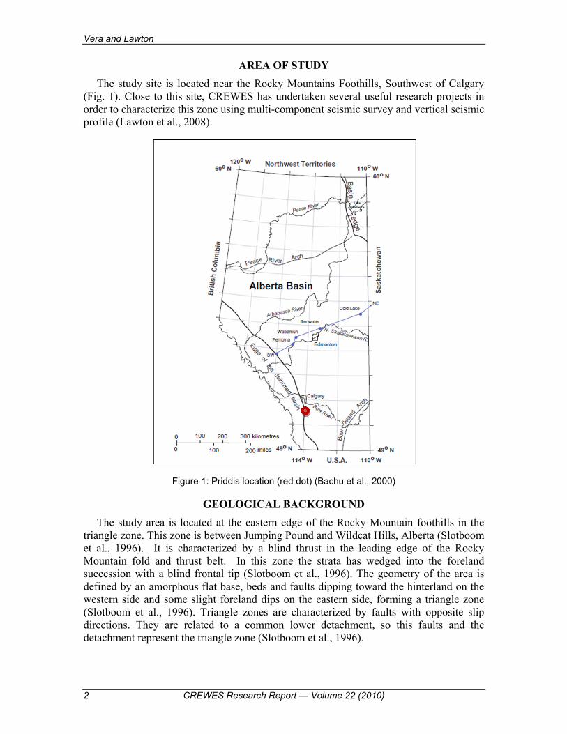
The study site is located near the Rocky Mountains Foothills, Southwest of Calgary (Fig. 1). Close to this site, CREWES has undertaken several useful research projects in order to characterize this zone using multi-component seismic survey and vertical seismic profile (Lawton et al., 2008).

Figure 1: Priddis location (red dot) (Bachu et al., 2000)

GEOLOGICAL BACKGROUND

The study area is located at the eastern edge of the Rocky Mountain foothills in the triangle zone. This zone is between Jumping Pound and Wildcat Hills, Alberta (Slotboom et al., 1996). It is characterized by a blind thrust in the leading edge of the Rocky Mountain fold and thrust belt. In this zone the strata has wedged into the foreland succession with a blind frontal tip (Slotboom et al., 1996). The geometry of the area is defined by an amorphous flat base, beds and faults dipping toward the hinterland on the western side and some slight foreland dips on the eastern side, forming a triangle zone (Slotboom et al., 1996). Triangle zones are characterized by faults with opposite slip directions. They are related to a common lower detachment, so this faults and the detachment represent the triangle zone (Slotboom et al., 1996).



Stratigraphic units

Three tectonostratigraphic units form the triangle zone in this area: Precambrian crystalline basement, Palaeozoic carbonate group and Mesozoic and Early Tertiary age clastic group (Slotboom et al., 1996). Figure 2 displays the stratigraphic column. Mesozoic stratigraphic sequences present the main deformations associated with the triangle zone formation. This section is composed by inter-bedded sandstone, siltstone, shales and coals from the foreland molasse strata. These sediments were uplifted due to a series of compressional episodes that shortened and thickened the sediments in the western margin of the craton during formation of the Canadian Cordillera (Stockmal et al., 1996).

Turonian (Cardium Formation) through Paleocene (Porcupine Hills Formation) exposed strata correspond with foreland siliciclastic basin that goes from marine to nonmarine and some fresh water limestone (Stockmal et al., 1996). The sequence of sediments is formed by: marine to nonmarine Milk River Formation and marine Pakowki Formation, nonmarine Belly River Group. St. Mary River Formation and Willow Creek Formation present a thickening due to its considerable deformation related to the upper detachment of the triangle zone.

Paskapoo Formation

The Paskapoo Formation represents the sequence of interest in this study. It is a Tertiary Formation (Fig.2) composed of mudstone, siltstone and sandstone, with subordinate limestone and coal. The sandstone grades to conglomerate in places, and bentonite beds are also present. The strata represent a foreland deposit of a siltstone- and mudstone-dominated fluvial system (Grasby et al., 2008)

This Formation constitutes an important ground water reservoir target having some qualities that make that possible as high-porosity coarse-grained sandstone channels (Grasby et al., 2008). The basal Haynes Member and western portion of the Paskpaoo Formation have higher sandstone volumes than other portions of the system (Grasby et al., 2008)

The Paskapoo Formation represents the youngest bed rock deposits in the Western Canada Sedimentary Basin having from 0 to 800m of thickness with a thinner section in the eastern part (see Figure 2) (Grasby et al., 2008). The deposits are distributed in an asymmetric foreland basin developed between the deforming mountain front and the adjacent craton due to the western thrusting of the Rocky Mountains (Grasby et al., 2008). The main source of sediments was the Palaeozoic-Mesozoic emerging mountains; compose by greenish sandy siltstone and mudstone, with light grey, thick-bedded sandstone deposited in nonmarine environments (Grasby et al., 2008). A plain zone where the strata are dipping westward, forming a homoclinal wedge into Alberta syncline, is called Paskapoo Sandstone, which has the most representative sandstone channels. Outside this sandy zone, the formation is composed for more than 50% of siltstone and mudstone (Grasby et al., 2008).

Vera and Lawton


Figure2: Stratigraphic sequence Rocky Mountains Foothills (Lawton, 1996)

FLUID SUBSTITUTION AND GASSMANN EQUATION

Fluid substitution modeling is an important tool in reservoir characterization. In this case, fluid substitution equations were used to predict and to evaluate CO2 injection in a specific area having well log information such as density and sonic.

Gassmann’s equation is one of the theories in fluid substitution modelling (Smith et al., 2003). Gassmann presents three major assumptions: the rock is homogeneous and isotropic, the pore space is completely connected and the fluids must be moveable. While many of the proposed models requires several and complicated inputs, Gassmann relations reflects the changes in P-wave and S-wave velocity due to saturation changes with simple inputs. Density and P-wave velocity logs are initial inputs and the constant parameters during substitution are matrix bulk modulus (Ko), frame or dry rock bulk modulus (K*), porosity (φ) and rock shear modulus (G) (Smith et al., 2003). The changes in fluid saturation will modify the fluid content and therefore, the bulk density (ρb) and fluid bulk modulus (Kfl) (Smith et al., 2003). Gassmann establishes empirical formulations that relate the saturated rock bulk modulus (Ksat) with porosity, dry rock bulk modulus, mineral matrix bulk modulus and pore filling fluid bulk modulus (Smith et al., 2003). The rock bulk modulus is calculated using the following expression:

𝐾 = K ∗ ( K∗ ) K∗ (1)

In order to resolve this formula it has to be accomplished a series of steps. Prior to apply Gassmann equation it is necessary define rock parameters such as bulk modulus, shear modulus and bulk density. Bulk modulus (K) is the ratio between stress increment (δε) and volume strain (δσ=∆V/V):

𝐾 = (2)

while shear modulus (G) is the ratio between shear strain and stress (Smith et al., 2003).



Bulk modulus (K) and shear modulus (G) can be related to compression velocity or P-wave velocity (Vp), shear velocity or S-wave velocity (Vs), and bulk density (ρb) all of them in saturated state, using these two equations:

𝐾 = 𝜌 𝑉 − 43 𝑉 (3) 𝐺 = 𝜌 𝑉 (4)

Since the shear modulus is insensitive to fluid changes, it will remain constant during the substitution (Smith et al., 2003). To calculate the bulk density (ρb) is used the following expression: 𝜌 = 𝜌 (1 − 𝜑) + 𝜌 𝜑 (5)

where ρ0 is matrix density, ρfl is fluid density and φ is porosity. Bulk density is going to change depending on the fluid saturation during the substitution.

The first step in Gassmann’s substitution is to define porosity values from well log data or to calculate them from density log values or any other log that could give this information (Smith et al., 2003). Rearranging equation 5 is possible to get porosity having density: 𝜑 = 𝜌 − 𝜌𝜌 − 𝜌 (6)

In order to substitute fluids it is necessary to establish their properties. In this case, the two fluids in discussion are water (or brine) and CO2. Density and bulk modulus values could be obtained from laboratory measurements but in most of the cases some empirical relations are use such as Batzle and Wang (1992) equations. They obtain the density and bulk modulus knowing temperature, pressure, gravity of the fluid (ºAPI in oil) and concentration (ppm in brine). With this input values a good approximation of fluid properties can be made at certain conditions. Some suggest that Batzle and Wang equations as well Gassmann relations, are created thinking in a gas-oil-water scenario, and they might not represent the reality of a CO2 fluid substitution (e.g. Xu, 2006). The resulting fluid bulk modulus (Kfl) after mixing two or more fluids, it is given by the expression:

𝐾 = (7)

where Si is the saturation and Ki is the bulk modulus of each fluid. This expression can be simplified in the following equation in the case of water and CO2 mix:

𝐾 = 𝑆𝐾 + (1 − 𝑆 )𝐾 (8)

where Sw is water saturation, Sc is CO2 saturation, Kw is water bulk modulus an Kc is CO2 bulk modulus.

Applying the same reasoning explained before, the fluid density (ρfl) is given by:

Vera and Lawton


𝜌 = ∑ 𝑆 𝜌 (9)

𝜌 = 𝑆 𝜌 + (1 − 𝑆 )𝜌 (10)

where ρi represent the density of each fluid, ρc is CO2 density and ρw water density.

Fluid bulk modulus and fluid density are going to reflect the fluid substitution changes and therefore, they are going to affect the model and define the variations.

To establish matrix characteristics, one needs to determine the matrix bulk modulus (Ko). These values are tabulated for main mineral components such as quartz and calcite among others. Most of the time, matrix is composed by different kind of minerals, and in case that fractional content information is available, the bulk modulus can be calculated using Voigt- Reuss-Hill (VRH) equation. This equation represents the average of the average, where is possible to obtain the bulk modulus (Kvrh) using Voigt and Reuss bulk modulus respectively (Kvoigt and Kreuss) (Smith et al., 2003):

𝐾 = 𝐾( ) + 𝐾( ) (11)

Reuss equation is the average of the harmonic mean (it represents the low band), and for the mixture of two components can be expressed as:

𝐾( ) = + (12)

On the other hand Voigt equation is the average of the arithmetic mean (it represents the upper band):

𝐾( ) = [𝐹 𝐾 + 𝐹 𝐾 ] (13)

K1, K2 is the bulk modulus of each mineral and F1, F2 is the fraction of mineral in the rock (Smith et al., 2003).

Another method used to calculate the matrix bulk modulus is Hashin and Shtrikman (1963) which assume a homogeneous mix of minerals and has narrower upper bound than Voigt but keep the lower bound of Reuss. Hashin-Shtrikman bounds can be obtained with the following equation:

𝑀 ± = 𝐾 ± + ± (14)

where MHS is the P-wave modulus and:

𝐾 ± = 𝐾 + (K K ) ( )(K G ) (15)

𝐺 ± = 𝐺 + (G G ) ( )(K G )G (K G ) (16)

K1 ,G1 and K2, G2 are the bulk modulus and shear modulus of each mineral. The relation between Vogit, Reuss and Hashin-Shtirikman curves can be seen in Figure 3.



To define frame properties or dry rock bulk modulus (K*), equation 1 is rearranged:

𝐾 ∗= (17)

Bulk modulus (Ksat) for the saturated rock obtained from equation 3, and the rest of the elements were obtained in previous steps (Smith et al., 2003). This property is calculated for a saturated rock and remains constant in fluid substitution. Shear modulus, matrix bulk modulus and porosity remain constant as well. Once that we have K* is possible calculate the rock bulk modulus (Ksat), using equation 3, for any water/ CO2 saturation values recalculating each time Kfl, ρfl, and ρb (Smith et al., 2003).

Figure3: Curves of Reuss, Voigt and Hashin-Shtrickman, showing bulk modulus variation with the porosity.

The final step consists of P-wave (Vp) and S-wave velocity (Vs) calculation using rock bulk modulus values (Ksat) for different CO2 saturation, using the following equations:

𝑉 = (18)

𝑉 = (19)

The shear modulus (G) calculated from equation 4 and the bulk density (ρb) recalculated from each saturation value using equation 5 (Smith et al., 2003).

The effects of fluid substitution in a certain formation or stratigraphic section could be evaluated by the changes suffered in P-wave velocity and S-wave velocity during the injection

Vera and Lawton


METHODOLOGY

Synthetic Seismogram Generation and Fluid Substitution Evaluation

Fluid substitution modelling was applied using the MILLAR 12-33-21-2W5 well log data. This is a well from Husky Oil and the data was recorded the presented data on June 19, 1980 (see figure 4). Hampson-Rusell PRO4D software was used to evaluate the data.

Figure 4: MILLAR 12-33-21-2W5 well location (GeoScout)

Figure 5 shows the logs provided by the borehole measurements. Track 1 is the gamma ray, track 2 is the density and track 3 is the P-wave velocity. Other logs were available but they don’t play an important role in fluid substitution.

From the Gamma Ray log it is possible to identify or at least estimate our objective. In this case, will be a “clean” sandstone portion of Paskapoo Formation. From previous geological information, it is known that this stratigraphical section corresponds with Tertiary sediments overlaying the Edmonton Formation. Identifying the Edmonton Fm Top, is inferred that the zone is located above it. In the GR log is possible to appreciate a low GR portion with shaly beds on top and base delimiting it. This zone goes from 380m to 425 m depth (see figure 5).

Once the objective was defined, the log data available was verified. Density log is recorded from 400 m, so the upper part was estimated using average values. That will be the only manipulation over real data. In further studies, lack of information could be solved with more complete log data.

Another aspect that can be appreciated is the increase of the GR in the lower zone of the section (425-440m), related with the decrease in the density log and in the P-wave velocity, that could be inferred as a coal layer.

MILLAR 12-33-2-2W5



Figure 5: Well logs: gamma ray (track 1), density (track 2) and P-wave (track 3)

From the density log, a porosity log was created using equation 4. Matrix density will be given by theoretical sandstone density value ρ=2650 Kg/m3 and as fluid density fresh water value ρ=1000 Kg/m3. From the P-wave velocity log it is possible to calculate the S-wave velocity using the empirical relation:

𝑉 = . (20)

where 1.9 is taken as a average value of Vp/Vs ratio in clastic sediments.

With all the elements, CO2 substitution was performed. First, complete water saturation condition is set. The first synthetic trace represents the 100% water saturation or 0% CO2 saturation. The subsequent traces are going to increase from 10 to 10 percent CO2 saturations till 100% stage. It is now possible to evaluate property changes due to CO2 substitution, specifically: velocity, time delay and amplitude of the wavelet.

Gassmann Fluid Substitution

Gassmann equations were used in order to estimate the changes in the P-wave velocity and the S-wave velocity after fluid substitution. Having density and sonic log values in the section identified as Paskapoo, an average value for both were obtained, which will represent the input in fluid substitution. The S-wave velocity at 100% water saturation is calculated using equation 20.

Vera and Lawton


In order to solve the Gassmann equation (see equation 1), was necessary to follow the steps described previously.

1) Calculate porosity value from equation 4 using the bulk density for 100% water saturation.

2) Define fluid properties: bulk modulus and density. As it was mentioned, these values depend on pressure and temperature and can be calculated with Batzle-Wang equations (Smith et al., 2003). Due to the lack of precise information the temperature (T) was estimated using geothermal gradient (Gt)

𝑇(410𝑚) = 𝐺 (410𝑚) + 𝑇(𝑠𝑢𝑟𝑓𝑎𝑐𝑒) (21)

and the pressure (P) was calculated using hydrostatic pressure gradient (Hp):

𝑃 = 𝐻 ℎ (22)

where Hp=9.792kPa/m and the chosen depth (h) is 410m.

The Geothermal Gradient considered is 27 degrees C/km in Alberta (Hitchon, 1984) and estimating a surface temperature of 15 degrees C, the approximated temperature in the middle of the sand is 25.8 degrees C. For the pressure, the column above the objective (h) will be 410m having a pressure of 4.015MPa.

With these values and Batzle-Wang calculations it is possible to obtain the CO2 bulk modulus Kc=0.02 GPa and density ρc =146.4 kg/m3. The expected phase of CO2 in a shallow formation would be gas, as we can see in the graph of Piri et al., 2005 (Fig. 6). The estimated water bulk modulus will be Kw=2.33 GPa, and fresh water density ρw= 1000 kg/m3 due to the lack of information about specific salinity of the area, nevertheless, studies such as the one presented by Grasby (2008) analyse the chemical composition of aquifers in Paskapoo formation, and in the south west Alberta it can be appreciated a higher concentration of calcium (~20mg/L).

Figure 6: Temperature and pressure phase diagram for pure carbon dioxide (Piri et al, 2005).



Having the individual characteristics of each fluid, Kfl and ρfl can be calculated using formulas 8 and 10 respectively, at different CO2 saturation states.

3) Define matrix properties: K0 matrix and ρ0 matrix. In this case we consider that the matrix is composed by perfect sandstone (quartz), so the K and ρ values are theoretical values of this mineral and they are not affected by pressure or temperature conditions. Since K0=37 GPa and ρ0=2650 kg/m3. According to lithological and stratigraphical characteristics, Paskapoo Formation contains clay and limestone.

4) Calculate bulk density by equation 5 with each new fluid density.

5) Calculate frame bulk modulus using equation 17 and introducing some of the previously mentioned values for 100% water saturation. Ksat is calculated with equation 3. K* value remain constant and is not affected by the substitution.

6) Calculate the rock bulk modulus (Ksat) with equation 1. This element and bulk density (ρb) is going to define the P-wave velocity further values. Ksat will vary according to the resultant Kfl.

7) Determine P-wave velocity and S-wave velocity values with equations 18 and 19, calculating previously the shear modulus G by equation 4. The bulk density and the rock bulk modulus were recalculated with each CO2 saturation values giving us eleven situations and eleven P-wave velocity and S-wave velocity values in each of them.

Seismic Modelling

Geological model

A 2D simple geological model of flat layers was created after estimating the P-wave velocity, the S-wave velocity and density parameters from the previous steps. The software utilized with this propose is NORSAR 2D. The interfaces between layers were estimated using the information provided by the well log dataset. The initial model parameters represent conditions prior to any CO2 injection scenario with 100% water saturation inside Paskapoo Formation. The model has an extension of 5 km and an injection zone of 1km located in the center of the model. This model attempts to characterize the changes in seismic data during various stages of CO2 injection (20%, 40%, 60%, 80% and 100% saturation). At the edges of the injection area, a 200 m transition zone was established; the parameters gradually range from the given specific CO2 saturation percentage to 0 % CO2.

Ray Tracing and Synthetic Seismogram Generation

Subsequent to generate the different models (before, during and after CO2 injection), it was necessary to obtain the seismic section (shot gather). The seismic survey parameters were: 120 channels, 10 meters between receivers (shot centered) and 40 meter spacing between shots. This geometry extended across the 5 km region. To perform ray-tracing was used the common shot ray-tracer with P-P reflections. After that it was possible to generate synthetic seismogram using a zero-phase Ricker wavelet with a frequency of 70 Hz. This frequency provided the resolution requirements in the area of interest:

Vera and Lawton


𝜆 = (23)

where V is the P-wave velocity in the layer of interest, f is the frequency and λ is the wave length. Calculating with the corresponding values:

𝜆 = . = 60.24 𝑚 (24)

𝑅𝑒𝑠𝑜𝑙𝑢𝑡𝑖𝑜𝑛 ~ = 15.06 𝑚 (25)

it was found that the resolution is approximately 15 m and the thickness of the layer is 45 m.

A total of six seismic files were generated and stored as SEG-Y files: 0%, 20%, 40%, 60% and 80% and 100% CO2. These sections represent the shot-gathers.

Processing of the Seismic Sections

In order to evaluate the model scenarios, it was necessary to generate the CDP gather and the CDP stack of the obtained shot gather sections. This process was performed using PROMAX software. The first step was the creation of the velocity model which is derived from the geological model with the correspondent P-wave velocity for each layer. For every case (before, during and after CO2 injection), a model was generated with corresponding velocity changes in the area of interest. After that, Normal Move Out (NMO) was applied to the reflectors in order to get the CDP gather. The final section or CDP stack was obtained by stacking the traces.

Comparison of the Different Sections

Once that the final stacked sections for the different saturation stages were obtained, it was possible to compare them and to evaluate the modelling results. The main alterations in the seismic reflectors are time shift and amplitude changes compared with the initial model stage.

The time delay was measured in the basal reflector. First it was necessary to calculate the theoretical time delay using the following equation:

ΔT = T – T = 2 H V – V (26)

where H is the thickness of the layer (45 m), V2 is the P-wave velocity of the injection zone for the given saturation stage and V1 is P-wave velocity for 0% CO2. Second, the time delay should be obtain from the CDP stack section. The 0% CO2 section is considered as the reference, and the time of the bottom reflector (at 425 m) was measured taking the reflector average time. The same procedure was applied for the rest of the sections. After getting all the values we should find the differences of each reflection times with the 0% CO2 case. These results should be compared with the theoretical calculations of time delay.



Another important evidence of different CO2 saturation values in the seismic sections is the amplitude variation. The difference between section with CO2 and the initial no CO2 condition, should be, qualitatively and quantitatively, appreciated performing the subtraction of the no CO2 section minus: 20%, 40%, 60% and 80% and 100% CO2, respectively. The interpolated amplitude value will be measured in the top reflector of the area of interest. This reflector is not affected by the low density coal layer below Paskapoo. The measured values should be compared with theoretical calculations of reflectivity.

In order to evaluate, theoretically, this amplitude changes, the Amplitude Vs Offset (AVO) analysis was applied. The method used was Shuey approximation which is less complex approximation to the Zoeppritz equation (Shuey, 1985). It calculates the reflection coefficient for diverse geological models and different angles of incidence (Shuey, 1985). This approximation is defined for two layers and before being expressed some variables have to be defined:

Vp1 is the P-wave velocity of layer 1 (layer above the injection zone)

Vp2 is the P-wave velocity of layer 2 (injection zone)

Vs1 is the S-wave velocity of layer 1 (layer above the injection zone),

Vs2 is the S-wave velocity of layer 2 (injection zone),

ρ1 is the density of the layer 1, ρ2 is the density of the layer 2, 𝑉 = is the P-wave velocity, ∆𝑉 = 𝑉 −𝑉 is the P-wave variation, 𝑉 = is the S-wave velocity, ∆𝑉 = 𝑉 −𝑉 is the S-wave variation, 𝜌 = is the density, ∆𝜌 = 𝜌 −𝜌 is the density variation,

σ1= ( ) is the Poisson ratio in layer 1 σ2= ( ) is the Poisson ratio in layer 2

𝜎 = is the Poisson ratio, ∆𝜎 = 𝜎 −𝜎 is the Poisson ratio variation, 𝐴 = 𝐵 −2(1 + 𝐵) , with 𝐵 = ∆ /∆ ∆

Finally Shuey’s approximation can be expressed as:

𝑅 = 𝑅 + 𝐴 R + ∆( ) sin θ + ∆V (tan θ − sin θ ) (27)

where:

Vera and Lawton


Ri is the reflection coefficient for the incident angle θi andcan be expressed as Rpp (only includes P-P reflection),

Ro is the reflection coefficient at zero offset

Shuey’s equation can be expressed as:

𝑅 = 𝐴 + 𝐵sin θ + C(tan θ − sin θ ) (28)

where A is the reflection coefficient at zero offset, B, called gradient and describes the small angle behaviour (<30 degrees) and C describe large angles (Brown et al., 2007). If the geometry of the model doesn’t cover more than 30 degrees the equation can be simplify:

𝑅 = 𝐴 + 𝐵sin θ (29) Beside the Shuey calculation, Zoeppritz 2.0 CREWES calculator was used in order to

estimate the AVO effect and compare with the Shuey’s results.

RESULT

Gassmann Fluid Substitution

After applying fluid substitution over 380-425m in MILLAR 12-33-21-2W5 well and after generating synthetic seismic traces for each CO2 saturation states, some alteration can be evaluated. Figure 7 shows GR (track1), porosity (track 2), density, P-wave velocity (track 3), S-wave velocity (track 4) and synthetic logs with 100% water saturation. In addition is displayed the synthetic seismogram at different CO2 saturation values, form 0 to 100 percent.

Figure 8 shows the synthetic seismogram with different saturation values. The variation between synthetic traces can be appreciated in the zone of fluid substitution (380-425m). Looking at the bsal reflector (425 m) a subtle time shift affects it from 0 to 100% CO2 saturation. The amplitude values changes across the substitution in the top reflector (380m) with CO2 increment (See Fig.9). Changes in the P-wave velocity correspond with the variations in traces (See Fig.10), there is an evident P-wave velocity reduction, highlighted at 390-400m. The main drop occurs from 0 to 20% CO2 saturation, but it can’t be recognized any major variation for higher saturation values.

Gassmann equations were developed using Microsoft Excel calculus sheet. Important results are the P-wave velocity, the S-wave velocity, the P-wave velocity change, the S-wave velocity change and Vp/Vs change, all of them for CO2 substitution from 0 to 100 percent saturation (See Table 1). The P-wave velocity values drop abruptly between 0 to 0.2 CO2 saturation, and starts to increase at 0.3 saturation, as shown in Figure 11. From equation 18, this is evident from the relation of P-wave velocity with Ksat and ρ bulk. With CO2 saturation increasing the rock bulk modulus (Ksat) decreases and therefore the P-wave velocity decreases too, but at the same time the bulk density (ρb) diminishes and due to its inverse relation with P-wave velocity will increase. From 0 to 0.2, the decrease in Ksat values is more representative than the decrease in ρb resulting in an overall decrease in the P-wave velocity, but from 0.3 CO2 saturation, the lower density values



cause a subtle increment in the P-wave velocity. The maximum P-wave velocity decrease is 7 %.

Figure 7: MILLAR 12-33-21-2W5 Logs: gamma ray (track 1), porosity (track 2), P-wave (track 3), density (track 3), S-wave (track 4), synthetic traces at different CO2 saturation values, and synthetic trace at 100 % water saturation.

Vera and Lawton


Figure 8: Synthetic seismogram at different saturation values. Zone of fluid substitution with blue parenthesis (380-425m). Time shift at 425 m with red line (basal reflector).

Figure 9: Synthetic traces, amplitude variation with increasing CO2 saturation



Figure 10: Synthetic traces, velocity variation with increasing CO2 saturation

a)

b)

Table 1: a) Gassmann fluid substitution results (380-425m). b) Input values.

Vera and Lawton


On the other hand, the S-wave velocity increase is directly proportional to CO2 saturation (see table 1) as shown in Figure 12. From equation 19, is possible to see that the S-wave velocity change depends only on bulk density variations since the shear modulus remains constant and it is not reflected by fluid substitution. However, the average increase of the S-wave velocity with respect to 100% water saturation is only 0.8%.

Figure 11: P-wave velocity change versus CO2 saturation

Figure 12: S-wave velocity change versus CO2 saturation

Vp/Vs values decrease with CO2 saturation due to the increase of Vs and a decrease in Vp (see Table 1) having a maximum decrease of 8%. Figure 13 shows a sharp drop from 0 to 0.1 CO2 saturation, becoming more linear for higher values. An extra element included in this table is the time delay calculated using equation 26. As CO2 saturation increases a time delay trough the reservoir is produced; it takes more time to the P-wave travel the through the zone of interest. In this case the thickness of the interval (h) is 45 m. The average two-way delay time is 1.6 ms.

-8.000

-7.000

-6.000

-5.000

-4.000

-3.000

-2.000

-1.000

0.000

0 0.1 0.2 0.3 0.4 0.5 0.6 0.7 0.8 0.9 1

Vp

cha

nge

(%)

CO2 Saturation

0.000

0.200

0.400

0.600

0.800

1.000

1.200

1.400

1.600

0 0.1 0.2 0.3 0.4 0.5 0.6 0.7 0.8 0.9 1

Vs

cha

nge

(%)

CO2 Saturation



Figure 13: P-wave velocity/S-wave velocity change versus CO2 saturation

Seismic Modelling

A 2D geological model generated for the area is shown in Figure 14. It is made up a total of 8 layers form 0 to 1 km depth. Paskapoo Formation is the fourth (4th) layer, represented with dark blue and is from 380-425 m. The parameters estimated from well information for each of the layers are listed in Table 2. The first layer parameters are approximate for shallow conditions. Figure 15 represents the same geological model but after CO2 injection. All the initial conditions remain constant changing the parameters in the zone of injection which is reflected as the green block in Figure 15. The two regions at each side are the transition zones. The parameters used in the injection area for the different saturation stages are summarized in Table 3.

Figure 14: 2D Geological model of the area. Layer 4 (in blue) represents Paskapoo Formation.

-9

-8

-7

-6

-5

-4

-3

-2

-1

0

0 0.1 0.2 0.3 0.4 0.5 0.6 0.7 0.8 0.9 1

Vp/

Vs

chan

ge (%

)

CO 2 Saturation

Vera and Lawton


Layer Vp (m/s) ρ(kg/m3)1 1900 23002 2546 22503 3498 23904 4212 25095 3326 18756 3710 24297 4019 23988 3739 3738

Table2: P-wave and density values for each layer in the geological model. Paskapoo Formation is the 4th layer (green label)

Figure 15: 2D Geological Model with the area of saturation in green. Transition zones are at both sides (pink and purple blocks respectively)

CO2 Saturation (%)

ρ (kg/m3)

Vp (m/s)

0 2509 421220 2495 390140 2480 390760 2466 391780 2451 3928

100 2436 3939

Table3: Density and P-wave velocity values in the injection zone for each saturation value

Six CDP stack seismic sections were generated for the conditions: 0%, 20%, 40%, 60%, 80% and 100% CO2 saturation. Figure 16 shows the 0% CO2 saturation prior to



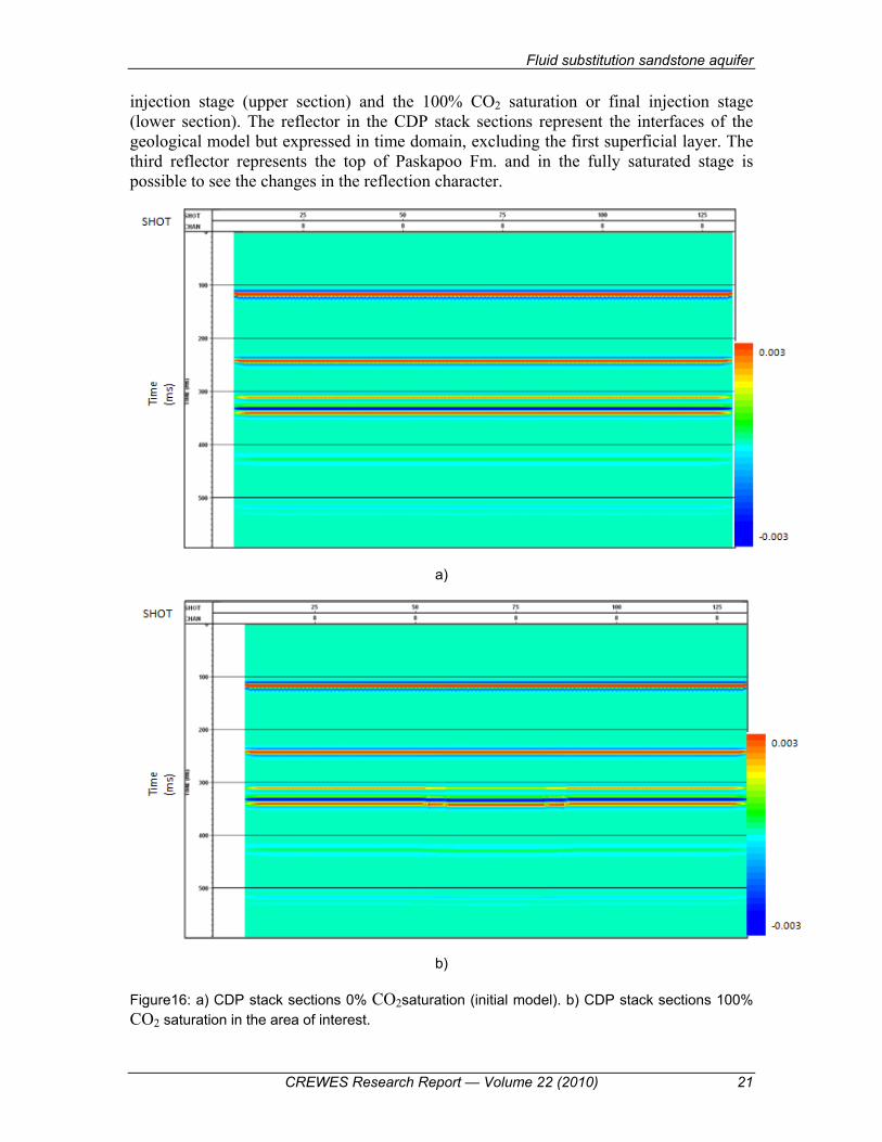
injection stage (upper section) and the 100% CO2 saturation or final injection stage (lower section). The reflector in the CDP stack sections represent the interfaces of the geological model but expressed in time domain, excluding the first superficial layer. The third reflector represents the top of Paskapoo Fm. and in the fully saturated stage is possible to see the changes in the reflection character.

a)

b)

Figure16: a) CDP stack sections 0% CO2saturation (initial model). b) CDP stack sections 100% CO2 saturation in the area of interest.

Vera and Lawton


Evaluating the time shift in the zone of injection, different time delay values were

found depending on the saturation. The theoretical values for time delay calculated with equation 26 are reflected in Table 4 with its respective tendency graph (Figure 17). On the other hand, in Table 5 we have the values for the time delay estimated from the CDP stack section and its graph as (Figure 18). The tendency of both curves is the same, it can be seen a sharp increase in the time delay for the 20% CO2 saturation stage, but the delay start a subtle decrease from 40%. There is an approximated difference of 0.07 ms between the theoretical and the observed values (higher values for the theoretical case). This difference might be attributed to the effect of the coal layer below Paskapoo. Between these two layers there is a high amplitude contrast that make difficult to obtain an accurate position in time of the basal reflector. Time delay vs. CO2 saturation curve has the opposite tendency than the P-wave velocity change vs. CO2 saturation curve. When the P-wave drops the time delay rises and when the P-wave velocity starts its subtle rising, time delay diminishes.

CO2 Saturation (%) dt(ms)0 0.00

10 1.6820 1.7030 1.6940 1.6750 1.6460 1.6170 1.5880 1.5590 1.51

100 1.48

Table 4: CO2 saturation values and theoretical calculated time delay (dt).

Figure 17: Theoretical time delay vs. CO2 saturation

0.00

0.50

1.00

1.50

2.00

0 10 20 30 40 50 60 70 80 90 100Tim

e D

elay

dt (

ms)

CO2 Saturation (%)



CO2 Saturation (%) dt(ms)0 0

20 1.0440 1.0260 0.9480 0.89

100 0.82

Table 5: CO2 saturation values and observed time delay (dt)

Figure 18: Observed time delay vs. CO2 saturation

The effect of the CO2 injection can be appreciated by subtracting each of the CDP stack sections from the 0% CO2 section. Figure 19 shows the difference between the 0% CO2 section and the 100% CO2 section. As is expected, the rest of the traces outside the area of interest were cancelled while the top and bottom reflectors of this region are highlighted due to the difference in amplitudes and travel times of the event from the base of the injection horizon.

0

0.2

0.4

0.6

0.8

1

1.2

0 10 20 30 40 50 60 70 80 90 100

Tim

e D

elay

dt (

ms)

CO2 Saturation (%)

Vera and Lawton


Figure 19: Difference between 0% CO2 and 100% CO2 saturation CDP stack sections.

Amplitude versus offset analysis

In order to evaluate the changes in amplitude versus offset (AVO) depending on the saturation percentage, Shuey’s approximation was applied. Taking equation 29; A, B and Rpp coefficients for the different CO2 saturation stages, were calculated (see table 6).The gradient B and the Rpp coefficient for the different stages is calculated with15 degrees of P-wave incidence as model case.

CO2 Saturation A (R0)

B (θ=15 degrees)

Rpp (θ=15 degrees)

0 0.117 -0.0121 0.1050.1 0.078 -0.0142 0.0640.2 0.076 -0.0142 0.0620.3 0.075 -0.0141 0.0610.4 0.074 -0.0141 0.0600.5 0.073 -0.0141 0.0590.6 0.072 -0.0140 0.0580.7 0.071 -0.0140 0.0570.8 0.071 -0.0139 0.0570.9 0.070 -0.0139 0.0561 0.069 -0.0138 0.055

Table 6: CO2 saturation stages with its correspondent A, B and Rpp values.

The values for the overlaying bed are: P-wave velocity of 3497 m/s (Vp1), S-wave velocity of 1665 m/s (Vs1) and a density of 2390 kg/m3 (ρ1).



Figure 20: Shuey’s approximation elements: A, B and Rpp vs. CO2 saturation (P-wave incidence angle was fixed at 15 degrees).

In Figure 20 are represented the values of Table 6. The first graphs, A (zero offset reflectivity coefficient) vs. CO2 saturation, shows that for higher concentrations of CO2 the amplitude will decrease. Zero offset reflectivity has a quick drop from 0% to 10% CO2 saturation having a subtle decrease in the subsequent stages. CO2 will reduce the bulk density and therefore the reflectivity contrast. In this sense the amplitude is going to be reduced with the increment of CO2 saturation.

The second graph, B (gradient) vs. CO2 saturation, shown a different tendency, having the same significant decrease from 0% to 10%, but starts subtle rise after 20% CO2 saturation similar Vp vs. CO2 saturation. Finally, the P-wave reflectivity coefficient (Rpp) vs CO2 saturation graph is similar to A vs. CO2 saturation, where the reflectivity values and therefore, the resulting amplitude values, will decrease with the increment of CO2 saturation, having the greater drop in the first 10 %.

Beside the theoretical calculation, the amplitude was estimated form the CDP stack section. Table 7 shows the relative values for amplitude decrease with the increment of CO2 saturation. In Figure 21 we have amplitude vs. CO2 saturation, presenting the same tendency than the theoretical curve.

Vera and Lawton


CO2 Saturation (%)

Amplitude (%)

0 10020 6440 6260 6180 60

100 57

Table7: Relative amplitude values measured from CDP stack sections with different CO2 saturation conditions

Figure 21: Amplitude vs. CO2 saturation (measured from CDP stack section).

After evaluating the changes in reflectivity due to CO2 saturation, the final Rpp was calculated with different angles of incidence to evaluate the changes of reflectivity with offset. Shuey’s approximation (equation 29) was applied for three CO2 saturation stages: 0%, 20% and 60%, taking a maximum angle of 25 degrees which is close to the incident angle for the maximum offset in this geometry.

Angle (Degrees) Rpp(0% CO2) Rpp(20% CO2) Rpp(60% CO2)

0 0.117 0.076 0.072 5 0.115 0.074 0.071

15 0.105 0.062 0.058 25 0.085 0.038 0.035

Table 8: Rpp coefficient values at different CO2 saturation stages (0%, 20% and 60%) and its changes with the angle of incidence.

0

20

40

60

80

100

0 10 20 30 40 50 60 70 80 90 100

Am

plit

ude

(%)

CO2 Saturation (%)



Figure 22: Rpp Vs Angle of incidence with different CO2 saturation stages (0%, 20% and 60%).

In Table 8 shows the Rpp values at the different stages (0%, 20% and 60%) and with different incidence angles. The graph presented in Figure 22 shows the curves at each saturation stage. The reflectivity diminishes with the increment in the incident angle. All the curves have the same tendency, but with the CO2 increment the reflectivity values decrease. The major drop occurs for 0% to 20%.

CONCLUSIONS

• Paskapoo Formation has suitable qualities for a test CO2 geological storage site; it has considerable section of clean sandstone and being a shallow objective will reduce monitoring complexities and cost.

• Gassmann theory is a practical and useful tool in fluid substitution models. Direct evaluation and synthetic seismogram variation reflects the effects of CO2 saturation. Applying this principle over a 380-425 m section it is possible to evaluate some changes. In the synthetic traces a time shift and amplitude variation is detectable in the area of interest. P-wave velocity drops quickly from 0 to 0.2 CO2 saturation, becoming more uniform at higher saturations.

• Applying Gassmann fluid substitution, the following was observed: average P-wave velocity decrease is 7%, average S-wave velocity increase is 0.8 %, average Vp/Vs decrease 8% and two-way time delay trough the reservoir is 1.6 ms. The Vs increase is directly proportional to the CO2 saturation. The decrease of Vp and density will represent a decrease in the impedance and therefore in the reflectivity contrast.

• Seismic modelling helped to simulate the conditions in the region of interest and the seismic changes during the different stages of CO2 injection (0%, 20%, 40%, 60%, 80% and 100% CO2 saturation). These variations can be seen in the injection zone inside the Paskapoo Formation. After performing the difference between traces the residual CDP stack section obtained highlights the injection zone.

0.000

0.050

0.100

0.150

0 5 10 15 20 25

R pp

Incident Angle (degrees)

Rpp Vs AngleRpp 0% CO2Rpp 20% CO2Rpp 60% CO2

Vera and Lawton


• Evaluating the time shift from the CDP stack sections, a delay was found in the basal reflector for 20% CO2 saturation condition (1.04 ms), but it started to diminish with the saturation increment. The observed values are coherent with the theoretical calculations. The time delay vs. CO2 Saturation has the opposite tendency than the Vp change vs. CO2 Saturation curve. The observed value for time delay is approximated 0.07 ms less than the expected value. This range of error could be a product of the reflection effect of the coal layer below the Paskapoo Formation.

• The amplitude will decrease with increasing CO2 saturation, having a major drop at 20 % CO2 saturation, according what it can be observe from CDP stack sections. The overlaying layer present lower velocity and density than Paskapoo Formation, so the increase in CO2 saturation will diminish the bulk density in the Formation, reducing the reflectivity contrast. Theoretical and observed data confirm this result.

• From Shuey’s approximation, it was found that the P-wave reflectivity coefficient decreases with the CO2 saturation increment. The major drop will occur at the first 20 % saturation, and it will have a slight decrease for the next stages. Evaluating the changes in reflectivity due to incident angle, it was found that for larger angles, the reflectivity decreases.

ACKNOWLEDGMENT

The authors would like to thank the Consortium for Research in Elastic Wave Exploration Seismology (CREWES), sponsors, staff and students. Software for the fluid replacement, modelling, synthetic generating and processing was provided to the University of Calgary by Hampson-Russell, Norsar2D, Promax and Vista.

REFERENCES

Bachu S., Michel Brulotte, Matthias Grobe and Sheila Stewart, 2000, Suitability of the Alberta Subsurface for Carbon-Dioxide Sequestration in Geological Media, Earth Sciences Report 2000-11

Batzle, M., and Wang, Z., 1992, Seismic properties of pore fluids: Geophysics, 57, 1396–1408. Brown, S. and Gilles Bussod, 2007, AVO monitoring of CO2 sequestration: A benchtop-modeling study,

The Leading Edge, 1576-1583. Castagna, J. P., and Smith, S. W., 1994, Comparison of AVO indicators: A modeling study: Geophysics,

59, no. 12, 1849–1855. Gassmann, F., 1951, Uber die Elastizitat Poroser Medien: Vier. Der Natur. Gesellschaft in Zurich, 96, 1–

23. Grasby S., Zhuoheng Chen, Anthony P. Hamblin, Paul R.J. Wozniak and Arthur R. Sweet, 2008,Regional

characterization of the Paskapoo bedrock aquifer system, southern Alberta, Can. J. Earth Science, 45, 1501-1516

Hashin, Z., and Shtrikman, S., 1963, A variational approach to the elastic behaviour of multiphase materials: J. Mech. Phys. Solids, 11, 127-140.

Hovorka, S. Surveillance of a Geologic Sequestration Project: Monitoring, Validation, Accounting. GCCC (Gulf Coast Carbon Center) Digital Publication Series #08-01, 2008.

Hitchom B., 1984, Geothermal gradients, hydrodynamics, and hydrocarbon occurrences, Alberta, Canada: AAPG Bulletin,1984, vol 68; no. 6, p. 713-743.

Lawton D., Malcolm B. Bertram, Robert R. Stewart, Han-xing Lu and Kevin W. Hall, 2008, Priddis 3D seismic Surrey and development of a training center, Crewes Research Report, vol 20.



Piri, M., Prevost, J. H., and Fuller, R., 2005, Carbon Dioxide Sequestration in Saline Aquifers: Evaporation, Precipitation and Compressibility Effects: Fourth Annual Conference on Carbon Capture and Sequestration DOE/NETL.

Shuey, R. T., 1985, A simplification of the Zoeppritz equations, Geophysics, 50, 509-614. Slotboom R., Donald C. Lawton and Deborah A. Spratt , 1996, Seismic interpretation of the triangle zone

at Jumping Pound, Alberta: Bulletin of Canadian Petroleum Geology, vol 44. no. 2, p. 233- 243. Smith T., Carl H. Sondergeld, and Chandra S. Rai, 2003, Gassmann fluid substitutions: A tutorial,

Geophysics, vol. 68, no. 2, p. 430-440. Sodagar T. and Dr. Don C. Lawton, 2009, Seismic modelling of fluid substitution in Redwater Reef:

Crewes Research Report, vol 21. Stockmal G., Paul A. MacKay, Don C. Lawton and Deborah A. Spratt, 1996, The Oldman Rirver triangle

zone: a complicated tectonic wedge delineated by new structural mapping and seismic interpretation: Bolletin Canadian Petroleum Geology, vol 44, no. 2, p. 202-214.

Xu H., 2006, Short Note Calculation of CO2 acoustic properties using Batzle-Wang equations: Geophysics, vol. 71, no. 2, p. F21-F23.

http://en.wikipedia.org/wiki/Priddis,_Alberta http://www.netl.doe.gov/technologies/carbon_seq/core_rd/CO2capture.html

virginia c. vera and don c. lawton - crewes.org · virginia c. vera and don c. lawton abstract...

Documents