virginia mazzini specific-ion effects in non-aqueous … virginia phd...here i investigate...
TRANSCRIPT

virginia mazziniS P E C I F I C - I O N E F F E C T S I NN O N - A Q U E O U S S O L U T I O N S


virginia mazziniS P E C I F I C - I O N E F F E C T S I NN O N - A Q U E O U S S O L U T I O N S
December 2017
A thesis submitted for the degree of Doctor of Philosophyof The Australian National University© Copyright by Virginia Mazzini 2017

Virginia Mazzini: Specific-ion effects in non-aqueous solutions, A thesis sub-mitted for the degree of Doctor of Philosophy of The Australian NationalUniversity © December 2017.
e-mail: [email protected]
This document was typeset using LATEX and Lorenzo Pantieri’s ArsClassica package,a reworking of the ClassicThesis style designed by André Miede, inspired to themasterpiece The Elements of Typographic Style by Robert Bringhurst.Graphics were typeset using the tikz package, to achieve continuity of the typo-graphic style in text and graphics. Calculations were performed, and plots made,in R (R Core Team, 2017), using mainly the packages plyr and ggplot2; the pack-age tikzDevice was employed to translate the R graphics into LATEX tikz-pgf com-mands.
The front cover displays the Coat of Arms of The Australian National University,stating the University motto ‘Naturam Primum Cognoscere Rerum’—‘First to learn thenature of things’ (Lucretius, De Rerum Natura, l. VI).

This thesis is an account of my own original research work, undertakenbetween May 2013 and December 2017 at the Department of Applied Math-ematics in the Research School of Physics and Engineering at the AustralianNational University (Canberra, Australia).Parts of the contents presented have been produced in collaboration withcolleagues, and published or submitted for publication in peer-reviewedjournals. These are listed in the section ‘List of Publications’ and are clearlymarked in the body of the document.None of this material has been submitted in whole or part to any other insti-tution for the award of a degree or diploma. To the best of my knowledge,this thesis contains no work previously published by another person, exceptwhere due reference is made in the text.This research is supported by an Australian Government Research TrainingProgram (rtp) Scholarship.This manuscript contains approximately 40000 words.
I acknowledge and celebrate the First Australians on whose traditional landsI have been living during the production of this thesis, and I pay my respectto the elders of the Ngunnawal people past and present.
Canberra, December 2017
Virginia Mazzini

A C K N O W L E D G E M E N T S
I am grateful to all that have supported me, professionally and/or personally,during this demanding journey.
I thank my supervisor Prof. Vince Craig for providing positive incentives,creative and honest scientific discussions, genuine advice, and for strivingto adapt his supervision methods to the different needs of his students. I amparticularly grateful for the opportunities of development and networkingProf. Craig has enabled me to attend, and for his commitment to promotingan inclusive and diverse research environment.
My advisor Prof. Pierandrea Lo Nostro has introduced me to the topic ofspecific-ion effects, and has been a participating mentor since my Masters’studies. I am thankful for the scientific guidance, the lifting conversations inmoments of discouragement, and for the light-hearted humour.
Dr. Drew Parsons, also in the role of advisor, has willingly given assistancein some more abstract aspects of my research. In addition, I am appreciativeof the fruitful discussions that I have shared with Dr. Andrea Salis duringhis time as a visiting fellow in the Department of Applied Mathematics; andof the caring advisory support and frank opinions provided by Prof. BarryNinham.
I also have received invaluable technical support for the completion ofmy work. I am indebted to Mr. Tim Sawkins and Mr. Ron Cruikshank atthe Department of Applied Mathematics for general technical support; toMr. David Anderson, Mr. Dennis Gibson and Mr. Luke Materne of the Re-search School of Physics and Engineering Electronics Unit at the anu — es-pecially for assembling the ‘button-bot’; to Ms. Bozena Belzowski, Mrs. AvisPaterson and Mr. Vance Lawrence at the anu Research School of Chemistryfor providing Blue Dextran; to Dr. Fouad Karouta from the Department ofElectronics Materials Engineering for granting access to experimental equip-ment.
On a personal note, I am blessed with the friendship and affection of many.I thank my parents Katia and Gino, for being devoted to us daughters, andfor educating us in the values of laicism, freedom, progress and solidarity.My sister Elisa, endless love and priceless wit. I look forward to reading yourthesis. Manuela and Massimo, for welcoming me as your own daughter andhosting me and chauffeuring me around Florence and Prato when I visited.
vii

Among my friends far and near, Daria, Jane, Viv, Anna, Lorena — offeringbanter, shenanigans and sisterhood. Namsoon, Martin, Muidh, Rohini, Al-ison, E-Jen, Rick, Matt, Ben and all the other fellow students and researchersin the Applied Mathematics Department.
Finally, Andrea, you had the wild idea of coming all the way down here toAustralia, and, in hindsight, you might have been right. Thanks for choosingto stand beside me every day. May all our dreams come true.
A B S T R A C T
Electrolyte solutions play a central role in life and technological processesbecause of their complexity. This complexity is yet to be described by a pre-dictive theory of the specific effects that different ions induce in solution. Thevast majority of investigations of specific-ion effects have been conducted inaqueous solutions. These studies have revealed that amongst the complexity,the effectiveness of the ions often follow trends that are apparent across anumber of very different experiments, revealing an underlying order, (e.g.the Hofmeister series). It is often assumed that water itself is intricatelyinvolved in these trends.
Here I investigate specific-ion effects in non-aqueous solvents rather thanwater. By extending the investigation to a number of non-aqueous solvents,the role of the solvent in specific-ion effect trends can be elucidated and abetter understanding of the general phenomenon gained.
Firstly, a more definite terminology is developed for describing the speci-fic-ion effects trends in order to address the current confusion in the liter-ature and provide a basis for the following investigations. An extensiveinvestigation of the scarce literature demonstrates that water is by no meansa special solvent with regards to ion-specificity, and that within the com-plexity there is universality. An investigation of electrostriction under theconditions of infinite dilution shows that the same fundamental specific iontrends are observed across all solvents, demonstrating that ion-specificityarises from the ions themselves. In this regard the influence of solvents, sur-faces and real concentrations of electrolytes can be seen as perturbations tothis fundamental series. Further work shows that for systems that are per-turbed, the trends in non-aqueous protic solvents can be expected to followthe same trend in water; and in aprotic solvents the cations are more likelyto adhere to the trend in water than the anions.
My experimental work focuses on specific-anion effects of seven Hofmeis-ter sodium salts in the solvents: water, methanol, formamide, dimethylsulfoxide and propylene carbonate. Two very different experiments wereperformed; the elution of electrolytes from a size-exclusion chromatographycolumn and an investigation of the electrolyte moderated swelling of a cat-ionic brush (pmetac) using a Quartz Crystal Microbalance (qcm). Thetrends observed are consistent across these experiments. A forward or re-verse Hofmeister series is observed in practically all salt-solvent combina-tions, and the reversal is attributed to the polarisability of the solvent.
ix

Finally, a qualitative model of ion specific trends is formulated, where thespecific-ion effects are fundamentally a property of the ion, and the associ-ated trends correspond to the Hofmeister series for anions and the lyotropicseries for cations. When the concentration is increased, or surfaces intro-duced, the effects of ion-ion interactions and ion-surface interactions canperturb the fundamental series. The perturbation of the series is related tothe proticity of the solvent for ion-ion interactions, whereas the polarisabilityof the solvent and ion are important when a surface is present. This work forthe first time individuates the principal properties of the solvent that affecttheir ordering: proticity and polarisability.

If you think education is expensive, try ignorance.
— Robert Orben


C O N T E N T S
list of figures xvii
list of tables xxi
list of acronyms & abbreviations xxiii
list of symbols xxv
list of publications xxxi
1 introduction 11.1 The importance of specific-ion effects 11.2 A brief historical account of sie 21.3 Theories of ion-specificity 31.4 An experimentalist’s point of view 51.5 Motivations for this work 61.6 Non-aqueous electrolytes 71.7 Outline of the thesis 7
2 literature review 92.1 Introduction 92.2 Manifestations of sie 102.3 Terminology 112.4 Characteristics of non-aqueous solvents 152.5 Methodology 172.6 Methanol 192.7 Formamide 212.8 N-methylformamide 222.9 N,N-dimethylformamide 232.10 Dimethyl sulfoxide 242.11 Additional solvents 252.12 Other investigations 282.13 An overall view 302.14 Summary 32
3 electrostriction 353.1 Motivation 353.2 Partial molar volumes and electrostriction 363.3 Methods 383.4 Results and discussion 413.5 Conclusions 54
4 volcano plots 574.1 Introduction 574.2 Energies related to the solvation process 58
xiii
xiv contents
4.3 The origin of volcano plots 594.4 The law of matching water affinities 614.5 Brief review of recent volcano plot studies 624.6 Results and discussion 684.7 Interpretation of volcano plots in solvents 734.8 Volcano plots in the ‘real world’ 814.9 Conclusions 84
5 experimental procedures 875.1 Experimental materials 875.2 Preparation of the salt solutions 905.3 The influence of trace quantities of water 935.4 Material incompatibilities with the solvents 97
6 chromatography of salts 996.1 Rationale 996.2 Size-exclusion chromatography in water 996.3 Description of the technique 1016.4 Experiment details 1036.5 Results and detailed discussion 1136.6 Summary 120
7 anion-specific polymer conformation 1237.1 Introduction 1237.2 Qcm for investigating polymer conformation 1247.3 Experiment details 1267.4 results and discussion 1317.5 Summary 134
8 an overall view 1358.1 A global depiction of sie in non-aqueous solvents 1358.2 The global experiment picture of anion trends 139
9 conclusions 1439.1 Further work 145
a electrostriction data 147a.1 Tabulation of the volumes 147
Bibliography for the current appendix 151a.2 Standard molar volumes of electrolytes 152a.3 Electrostrictive volume of electrolytes 154a.4 Normalised electrostrictive volumes 156
b volcano plots 159b.1 Aqueous ionic radii versus ab initio radii 159b.2 Lines highlighting cation trends 160b.3 Lines highlighting anion trends 164b.4 Solubilities of electrolytes in solvents 169
c osmotic and activity coefficients 171c.1 Fitting models and coefficients 171
contents xv
c.2 Plots 180Bibliography for the current appendix 186
d solubility data collection 191Bibliography for the current appendix 200
e custom conductivity cell 203
f effect of water impurities on sec and qcm experiments 205f.1 Size-exclusion chromatography 205f.2 Polymer conformation by qcm 208f.3 Conclusions 208
g a summary of unsuccessful approaches 209g.1 Standard molar volume measurements 209g.2 Turbidimetry 212g.3 Nmr T2 relaxation times of salt solutions 212g.4 Swelling of commercial hydrogels 212
bibliography 213


L I S T O F F I G U R E S
Figure 1 Hofmeister and lyotropic series of ions 13Figure 2 concentration dependence of electrostriction 38Figure 3 electrostrictive volumes scheme 39Figure 4 intrinsic volumes of electrolytes 41Figure 5 standard molar volumes of electrolytes in water 42Figure 6 electrostrictive volumes of electrolytes in water 48Figure 7 normalised electrostriction in water 49Figure 8 Born-Haber cycle of the solvation-related enthalpies 59Figure 9 volcano plots, free energies, cation trends 71Figure 10 radii volcano plots, enthalpies, cation trends 74Figure 11 radii volcano plots, free energies, cation trends 75Figure 12 protic volc. p. polyatomic anions, enthalp., cat. trends 77Figure 13 aprotic volc. p. poly. anions, enthalp., cat. trends 78Figure 14 radii protic volc. p., poly. anions, enthalp., cat. trends 79Figure 15 radii poly. anions aprot. volc. p., enthalp., cat. trends 80Figure 16 volcano plots, activity coefficients, cation trends 83Figure 17 molecular models of the experiments chemicals 89Figure 18 scheme of the chromatography experiment setup 104Figure 19 custom-made conductivity detector calibration curves 106Figure 20 chromatogram of sodium electrolytes in water 114Figure 21 chromatogram of sodium electrolytes in meoh 116Figure 22 chromatogram of sodium electrolytes in fa 117Figure 23 chromatogram of sodium electrolytes in dmso 119Figure 24 chromatogram of sodium electrolytes in pc 120Figure 25 summary of sec retention factors 121Figure 26 pmetac skeletal structural formula 123Figure 27 qcm shifts, dependence on salt concentration 129Figure 28 qcm shifts, brush-coated sensor versus bare sensor 130Figure 29 qcm, pmetac brush net response to concentration 130Figure 30 qcm, solvent-dependent effect of NaClO4 on pmetac 131Figure 31 summary of qcm shifts in all solvents 133Figure 32 qcm, ∆D3 versus −∆F3 plot 134Figure 33 standard molar volumes of electrolytes in meoh 152Figure 34 standard molar volumes of electrolytes in etoh 152Figure 35 standard molar volumes of electrolytes in fa 152Figure 36 standard molar volumes of electrolytes in nmf 152Figure 37 standard molar volumes of electrolytes in eg 152Figure 38 standard molar volumes of electrolytes in pc 153Figure 39 standard molar volumes of electrolytes in ec 153Figure 40 standard molar volumes of electrolytes in dmso 153Figure 41 standard molar volumes of electrolytes in ace 153Figure 42 standard molar volumes of electrolytes in mecn 153Figure 43 standard molar volumes of electrolytes in dmf 153
xvii
xviii list of figures
Figure 44 electrostrictive volumes of electrolytes in meoh 154Figure 45 electrostrictive volumes of electrolytes in etoh 154Figure 46 electrostrictive volumes of electrolytes in fa 154Figure 47 electrostrictive volumes of electrolytes in nmf 154Figure 48 electrostrictive volumes of electrolytes in eg 154Figure 49 electrostrictive volumes of electrolytes in pc 155Figure 50 electrostrictive volumes of electrolytes in ec 155Figure 51 electrostrictive volumes of electrolytes in dmso 155Figure 52 electrostrictive volumes of electrolytes in ace 155Figure 53 electrostrictive volumes of electrolytes in mecn 155Figure 54 electrostrictive volumes of electrolytes in dmf 155Figure 55 normalised electrostriction in meoh 156Figure 56 normalised electrostriction in etoh 156Figure 57 normalised electrostriction in fa 156Figure 58 normalised electrostriction in nmf 156Figure 59 normalised electrostriction in eg 156Figure 60 normalised electrostriction in pc 157Figure 61 normalised electrostriction in ec 157Figure 62 normalised electrostriction in dmso 157Figure 63 normalised electrostriction in ace 157Figure 64 normalised electrostriction in mecn 157Figure 65 normalised electrostriction in dmf 157Figure 66 hydrated versus ab-initio radii of ions 159Figure 67 volcano plots, protic, enthalpies, cation trends 160Figure 68 volcano plots, aprotic , enthalpies, cation trends 160Figure 69 exploded volcano plots, protic, enthalpies, cation trends 161Figure 70 exploded volcano plots, aprotic , enthalpies, cat. trends 161Figure 71 volcano plots, osmotic coefficients, cation trends 162Figure 72 poly. anions volcano plots, osmotic coeff., cation trends 163Figure 73 poly. anions volcano plots, activity coeff., cation trends 163Figure 74 volcano plots, protic, enthalpies, anion trends 164Figure 75 volcano plots, aprotic , enthalpies, anion trends 164Figure 76 volcano plots, protic, free energies, anion trends 165Figure 77 volcano plots, aprotic , free energies, anion trends 165Figure 78 radii volcano plots, protic, enthalpies, anion trends 166Figure 79 radii volcano plots, aprotic , enthalpies, anion trends 166Figure 80 radii volcano plots, protic, free energies, anion trends 167Figure 81 radii volcano plots, aprotic , free energies, anion trends 167Figure 82 volcano plots, osmotic coeff., anion trends 168Figure 83 volcano plots, activity coeff., anion trends 168Figure 84 electrolyte solubility in protic solvents 169Figure 85 electrolyte solubility in aprotic solvents 170Figure 86 osmotic coeff. of alkali metal halides 180Figure 87 activity coeff. of alkali metal halides 181Figure 88 osmotic coeff. of salts with polyatomic anions 182Figure 89 activity coeff. of salts with polyatomic anions 183Figure 90 osmotic coeff. of salts with polyatomic cations 184Figure 91 activity coeff. of salts with polyatomic cations 185Figure 92 schematics of the custom conductivity cell 203

list of figures xix
Figure 93 effect of water content on sec peaks in meoh 206Figure 94 effect of eluent water content on sec peaks in pc 206Figure 95 effect of sample water content on sec in pc 207Figure 96 effect of water content on sec peaks in dmso 207Figure 97 effect of water content on qcm shifts in meoh 208Figure 98 density of salt solutions versus salt concentration 210Figure 99 density change of solutions for 0.01mol dm−3 salts 211


L I S T O F TA B L E S
Table 1 Hofmeister original experiment series 3Table 2 physical properties of the solvents investigated 16Table 3 specific-ion effects series in water 18Table 4 sie series in meoh 19Table 5 additional sie series in meoh 20Table 6 sie series in fa 21Table 7 sie series in nmf 23Table 8 sie series in dmf 24Table 9 sie series in dmso 25Table 10 sie series in etoh 26Table 11 sie series in pc and ec 27Table 12 additional sie series in pc and ec 28Table 13 summary of sie series in different solvents 31Table 14 anion sie trends in standard molar volumes 43Table 15 cation sie trends in standard molar volumes 44Table 16 anion sie trends in electrostrictive volumes 46Table 17 cation sie trends in electrostrictive volumes 47Table 18 anion sie trends in the normalised electrostriction 51Table 19 cation sie trends in normalised electrostriction 52Table 20 summary of volcano plots reported in the literature 65Table 21 specifications of the electrolytes used in experiments 88Table 22 oven drying protocol for the electrolytes 88Table 23 technical specifications of the solvents investigated 90Table 24 solubility of electrolytes in non-aqueous solvents 92Table 25 summary of the electrolytes investigated per solvent 93Table 26 contaminant water to ion ratio 94Table 27 size of investigated ions and solvent molecules 100Table 28 sec column size in different solvents 110Table 29 summary of the anion-specific trends from experiment 139Table 30 ab initio static ionic polarisabilities 141Table 31 intrinsic, standard, electrostrictive and normalised volumes 147Table 32 Pitzer model fitting coeffs. in non-aqueous solvents 173Table 33 Pitzer-Archer model coeffs. in non-aqueous solvents 177Table 34 Polynomial fitting coefficients non-aqueous solvents 177Table 35 Pitzer coefficients for electrolytes in water 178Table 36 literature salt solubility in non-aqueous solvents 191
xxi


A C R O N Y M S & A B B R E V I AT I O N S
1pentoh 1-pentanol (pentan-1-ol). 1982buoh 2-butanol (butan-2-ol). 1922proh 2-propanol (propan-2-ol). 16, 173, 177, 199
ace acetone (propan-2-one). 16, 25, 30–32, 38, 42–47, 50–52, 150, 153, 155, 157, 173, 191
acs American Chemical Society. 88, 90
buoh butanol (butan-1-ol). 70, 191, 192
dlvo Derjaguin, Landau, Verwey, Overbeek. 4dma N,N-dimethylacetamide. 16, 173, 192dmc dimethyl carbonate. 173dme dimethoxyethane (1,2-dimethoxyethane). 173dmf N,N-dimethylformamide. 16, 23, 24, 26, 30–32,
38, 43, 44, 46, 47, 51, 52, 95, 150, 151, 153, 155,157, 173, 192, 193
dmso dimethyl sulfoxide. 7, 16, 24–26, 29–32, 38, 43,44, 46, 47, 51, 52, 83, 90, 91, 93–95, 97, 99, 100,103, 106, 109, 110, 112, 113, 116, 119–121, 127,128, 132, 134, 139–142, 144, 149, 150, 153, 155,157, 162, 163, 168, 173, 174, 177, 193, 205, 207
ec ethylene carbonate (1,3-dioxolan-2-one). 16,25–28, 30–32, 38, 42–44, 46, 47, 51, 52, 66, 68,83, 149, 153, 155, 157, 162, 168, 174, 177, 193
eg ethylene glycol (ethane-1,2-diol). 16, 25, 28, 30,31, 38, 42–44, 46, 47, 51, 52, 70, 148, 149, 152,154, 156, 193
etoh ethanol. 7, 16, 25–27, 29–31, 38, 43–47, 51, 52,148, 152, 154, 156, 174, 177, 193, 194
fa formamide. 7, 16, 21, 22, 24, 28, 30–32, 38, 43–47, 51, 52, 70, 90, 93, 94, 97, 99, 100, 103, 106,109, 110, 112, 113, 116–119, 121, 122, 127, 128,132, 134, 139–142, 144, 148, 152, 154, 156, 194,212
xxiii
xxiv acronyms & abbreviations
fep fluorinated ethylene propylene. 98, 105ft-ir Fourier-transform infrared spectroscopy. 28,
102
i-buoh iso-butanol (2-methylpropan-1-ol). 192i-pentoh iso-pentanol (3-methylbutan-1-ol). 198
kf Karl Fischer. 90, 91, 94–97, 205
lmc limiting molar ionic conductivity. 15, 18, 19,21–27, 30–32, 48, 53, 118, 122
lmwa law of matching water affinities. 8, 29, 37, 57,60–64, 66–68, 81, 82, 84, 89, 101, 118, 124, 143,172
md molecular dynamics simulations. 4, 64mecn acetonitrile. 7, 16, 25, 29–31, 38, 43, 44, 46, 47,
51, 52, 85, 95, 141, 150, 153, 155, 157, 174, 194,195
meno2 nitromethane. 25, 30–32, 141, 195meoh methanol. 7, 16, 19–21, 29–32, 38, 43–47, 51, 52,
67, 70, 82, 83, 85, 90, 93–97, 99, 100, 103, 105–107, 109–113, 115–117, 119–122, 127, 130–134,139–141, 144, 147, 148, 152, 154, 156, 162, 168,174, 175, 177, 195–197, 205, 206, 208, 209, 211,212
mhc constant pressure standard partial molar heatcapacity of the ion. 18–21, 23–27, 31, 32, 48
mrt nmr molecular reorientation time. 18–25, 31msa- methanesulfonate. 28
nma N-methylacetamide. 83, 141, 162, 163, 168,175–177, 197
nmf N-methylformamide. 16, 22–26, 30–32, 38, 43–47, 51, 52, 83, 84, 150, 152, 154, 156, 162, 168,176, 197
nmr nuclear magnetic resonance. 17, 20, 29, 61, 102,111, 125, 145, 212
pc propylene carbonate (4-methyl-1,3-dioxolan-2-one). 7, 16, 25–28, 30, 31, 38, 43, 44, 46, 47, 51,52, 66, 68, 72, 82, 83, 90, 93–95, 97, 99, 100, 103,109–113, 120, 121, 127, 129, 131, 132, 134, 139–141, 144, 149, 153, 155, 157, 162, 168, 176, 197,198, 205–207, 212
list of acronyms & abbreviations xxv
peek polyether ether ketone. 105pmetac poly(2-methacryloyloxyethyl-trimethyl-
ammonium chloride. 123, 124, 127, 129–134,140
proh 1-propanol (propan-1-ol). 16, 25, 30, 31, 72, 198,199
ptfe polytetrafluoroethylene. 98, 105, 106, 108, 128
qcm quartz crystal microbalance. 8, 91, 95, 97, 98,122, 124, 126–129, 131, 132, 134, 139, 140, 205,208
qcm-d quartz crystal microbalance with dissipationmonitoring. 125–127
rdd relative limiting static dielectric decrement. 18,19, 21–23, 31, 32
sec size-exclusion chromatography. 8, 95, 98, 99,101, 102, 114, 115, 120–122, 134, 138–140, 144,203, 205, 206
sie specific-ion effects. 1–12, 14, 15, 17, 19–28, 30–33, 35, 37, 43–47, 51–55, 57, 62, 64, 84, 85, 87,89, 90, 93–95, 99, 113, 122, 131, 132, 134–145,205
sulf sulfolane (tetrahydrothiophene 1,1-dioxide).163, 176, 177
t-buoh tert-butanol (2-methylpropan-2-ol). 141, 192
vbc viscosity B-coefficients (see Bη). 15, 18, 19, 21–27, 30–32, 48, 53, 83


L I S T O F S Y M B O L S
α static polarisability. 16, 141αp isobaric expansivity. 211AN Gutmann-Mayer acceptor number. 16, 17, 19,
70
Bη B-coefficients from the empirical Jones-Doleviscosity equation. 37, 48, 53, 61, 65–67, 83,85
ci amount-of-substance concentration of solute i,units moldm−3. 90, 210–212
CN coordination number. 65
Dn QCM dissipation factor of the overtone n2Γn/fn. 125, 126
∆Dn shift of — . 126, 128, 129, 132, 134DN Gutmann donor number. 15, 16, 19, 70
η viscosity. 16ε0 electric constant or vacuum permittivity,
8.854× 10⁻¹² Fm−1. 171εR relative permittivity. 16, 38, 60, 171e elementary charge, 1.602 176 634× 10−19C. 60,
171
fn QCM resonance frequency of the overtone n.125, 126
∆fn shift of the — . 126, 128–131, 133, 134, 208∆Fn normalised — — . 129–134, 208
γ activity coefficient. 82, 83, 163, 168, 171–176,181, 183, 185
Γn QCM half-height half-bandwidth of the over-tone n. 125
∆abs. hydr.G−◦ absolute standard molar Gibbs free energy of
hydration (solvation in water). 65∆abs. soln.G molar Gibbs free energy of solvation. 58∆abs. soln.G
−◦ absolute standard — . 58, 70, 71, 78, 165∆fG
−◦ standard molar Gibbs free energy of formation.58
xxvii
xxviii list of symbols
∆hydr.G−◦ standard molar Gibbs free energy of dissolu-
tion in water. 65∆soln.G
−◦ standard molar Gibbs free energy of dissolu-tion. 58, 69, 71, 75, 78, 80, 165, 167
∆abs. hydr.H−◦ absolute standard molar enthalpy of hydration
(solvation in water). 65∆abs. soln.H molar enthalpy of solvation. 58∆abs. soln.H
−◦ absolute standard — . 58, 59, 70, 77, 160, 164∆fH
−◦ standard molar enthalpy of formation. 58, 59,69
∆hydr.H molar enthalpy of dissolution in water. 60∆hydr.H
−◦ standard molar — . 65, 69∆soln.H
−◦ standard molar enthalpy of dissolution. 58, 59,69, 74, 77, 79, 160, 164, 166
k Boltzmann constant, 1.381× 10⁻²³ J K−1. 171Ka association constant. 65Kav size exclusion chromatography available reten-
tion factor. 102, 111, 115Kd dissociation constant. 65Ksec size exclusion chromatography retention
factor. 101, 102, 111, 113, 120, 121kT isothermal compressibility. 16, 38
µ dipole moment. 16Mi molar mass of species i in gmol−1. 3, 16, 40,
100, 111, 115, 209–211mi molality of solute i, units molkg−1. 90, 171–
185, 210
νi stoichiometric coefficient of species i. 3Na Avogadro constant 6.022× 10²³mol−1. 171N% electrostrictive volume normalised by the in-
trinsic volume. 49–53, 147–151, 156, 157ni number of moles of species i in mol. 36, 94,
209, 210
π 3.1415926536. 100, 125, 171φ osmotic coefficient. 65, 66, 162, 163, 168, 171,
172, 180, 182, 184P pressure. 36, 209
ρ∗i density of a pure substance i. 171, 210, 211
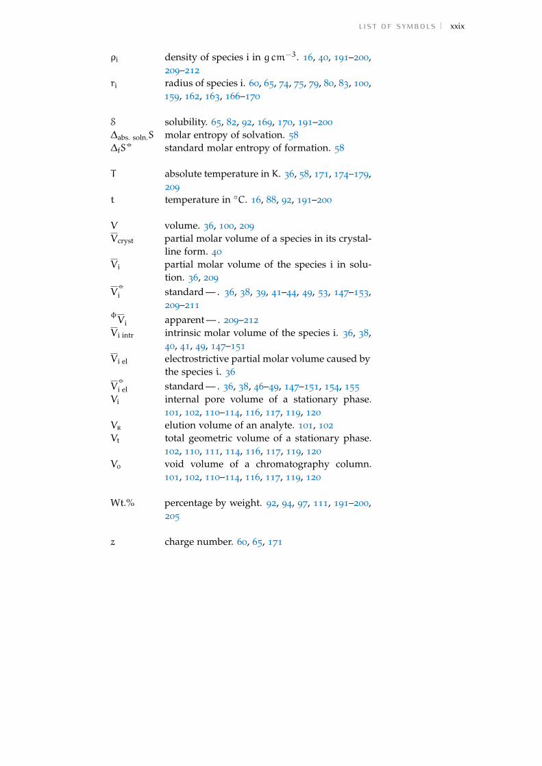
list of symbols xxix
ρi density of species i in g cm−3. 16, 40, 191–200,209–212
ri radius of species i. 60, 65, 74, 75, 79, 80, 83, 100,159, 162, 163, 166–170
S solubility. 65, 82, 92, 169, 170, 191–200∆abs. soln.S molar entropy of solvation. 58∆fS
−◦ standard molar entropy of formation. 58
T absolute temperature in K. 36, 58, 171, 174–179,209
t temperature in ◦C. 16, 88, 92, 191–200
V volume. 36, 100, 209Vcryst partial molar volume of a species in its crystal-
line form. 40V i partial molar volume of the species i in solu-
tion. 36, 209V−◦i standard — . 36, 38, 39, 41–44, 49, 53, 147–153,
209–211φV i apparent — . 209–212V i intr intrinsic molar volume of the species i. 36, 38,
40, 41, 49, 147–151V i el electrostrictive partial molar volume caused by
the species i. 36V−◦i el standard — . 36, 38, 46–49, 147–151, 154, 155Vi internal pore volume of a stationary phase.
101, 102, 110–114, 116, 117, 119, 120Vr elution volume of an analyte. 101, 102Vt total geometric volume of a stationary phase.
102, 110, 111, 114, 116, 117, 119, 120V0 void volume of a chromatography column.
101, 102, 110–114, 116, 117, 119, 120
Wt.% percentage by weight. 92, 94, 97, 111, 191–200,205
z charge number. 60, 65, 171


L I S T O F P U B L I C AT I O N S
Part of the work presented in this thesis has been published in the followingpapers:
Mazzini, V. and V. S. J. Craig2016 ‘Specific-ion effects in non-aqueous systems’, Curr. Opin. Colloid In-
terface Sci. 23, pp. 82–93, doi: 10.1016/j.cocis.2016.06.009.2017 ‘What is the fundamental ion-specific series for anions and cations?
Ion specificity in standard partial molar volumes of electrolytes andelectrostriction in water and non-aqueous solvents’, Chem. Sci. 8 (102017), pp. 7052–7065, doi: 10.1039/C7SC02691A.
2018 ‘Volcano plots emerge from a sea of non-aqueous solvents: The lawof matching water affinities extends to all solvents’, Submitted.
Mazzini, V., G. Liu and V. S. J. Craig2018 ‘Probing the Hofmeister series beyond water: Specific-ion effects in
non-aqueous solvents’, J. Chem. Phys. 148, 22, p. 222805, doi: 10.
1063/1.5017278.
xxxi


1 I N T R O D U C T I O N
The phrase ‘specific-ion effects (sie)’ encompasses all those cases where aproperty of an electrolyte solution, or the behaviour of a substance dissolvedtherein, depends on the particular cations and anions present beyond theirelectrostatic charge.
1.1 the importance of specific-ion effectsBetween the years 2000 and 2017, Web of Science™ indexes more than 1700publications investigating sie, that span across (bio)chemistry, (bio)physics,materials science, biotechnology, pharmacology, engineering, medicine, wa-ter resources and plant science. This interdisciplinary interest in sie stemsfrom the fact that electrolyte solutions are omnipresent: pure, neat watercontaining no dissolved salts is extremely rare in nature.
Salts are what enables the specificity and complexity of interactions in lifeprocesses. Everyone is aware of the essential role water has for life, but itis often overlooked that this water must be salty to be of any use: drink-ing demineralised water for long periods of time has deleterious effects onhealth due to osmotic shock and disruption of the body homeostasis mechan-isms (Kozisek, 2005). The details of ‘life’ is one of the most pressing researchtopics. Untangling its mechanisms and one day explaining its mystery is amajor ambition of scientific progress. This cannot be achieved without ac-knowledging the importance of salts for life: ions interact with proteins andaffect their solvated structure (Baldwin, 1996; Y. Zhang and Cremer, 2006);the activity of enzymes is salt-dependent (Bilanicová et al., 2008). Strikingexamples are provided by the fields of medicine and biology (Lo Nostroand Ninham, 2012). The fine-tuned equilibrium that allows the human bodyto function largely relies on the specificity allowed by electrolytes. For in-stance, intravenous injections of NaCl and KCl solutions, that differ only bythe cations they contain, both of charge +1, have dramatically distinct effectson a subject. The first one is known as saline solution, and can be injectedto treat dehydration. The latter instead alters the resting potential of thecardiac muscle and can quickly induce death by cardiac arrest (Weidmann,1956). Strict protocols are constantly discussed to avoid accidental adminis-tration of the latter to a patient (Reeve et al., 2005). An extensive account of
1
2 introduction
sie in biology can be found in: Kunz (2010), Lo Nostro and Ninham (2012)and Ninham and Lo Nostro (2010).
Ions have a fundamental role in climate and natural equilibria as well. Sea-water is quite rich in a variety of ions, and as a consequence foams more thanfreshwater. One of the causes of the foaming of sea water (pollution and al-gae aside) is the presence of salts that inhibit bubble coalescence (Craig, Nin-ham et al., 1993a). Salts also reduce the solubility of gases in water (Millero,Huang et al., 2002a,b) and therefore affect aquatic life.
Important sie are also observed in a vast variety of other settings, suchas the processing of colloids, where the stability (Lyklema, 2009) and rhe-ological behaviour of the system can be controlled (Franks, 2002; Frankset al., 1999). Also, the supramolecular self-assembly of surfactants is salt-dependent (Lo Nostro, Ninham, Ambrosi et al., 2003; Lo Nostro, Ninham,Milani et al., 2006). The above have consequences in applications such asmineral processing and wastewater treatment, and also in drug deliveryand in food processing (cheesemaking for instance). In addition, polymerconformations show rich ion-specificity (Y. Zhang and Cremer, 2006), withconsequences for instance in the development of responsive surface coat-ings (Azzaroni et al., 2005; G. Liu and G. Zhang, 2013; Willott et al., 2015;Y. Zhang, Furyk et al., 2005). Finally, sie are also relevant in corrosion kinet-ics (Trompette, 2015).
1.2 a brief historical account of sieThe realisation that the electrostatic charge of an ion is not sufficient to de-scribe the properties of its solutions occurred early on, but the theoreticalconnection of solution behaviour to the fundamental properties of the elec-trolytes remains a work in progress.
Although Poiseuille already had worked on the electrolyte-dependent vis-cosity of salt solutions (Kunz, 2009), the work of Franz Hofmeister and col-laborators at the end of the 19th century (Hofmeister, 1888a,b) is consideredthe starting point of the topic of sie in contemporary scientific literature.An English translation of this landmark work is available (Kunz, Henle etal., 2004).
Hofmeister and co-workers observed that different salts had a differentpower to precipitate egg white proteins (globulins and albumins, the firstprecipitate at lower salt concentration) out of solution. The ordering thatemerges is reported in Table 1. The precipitating power of the salts in thetable diminishes in going from left to right and top to bottom. This regu-larity was highlighted by Hofmeister who noted that the ability of the saltto precipitate proteins depends both on the anion and cation (Kunz, Henle

1.3 theories of ion-specificity 3
Table 1: Values from Hofmeister’s original study on the precipitation of eggglobulin (Hofmeister, 1888a; Kunz, Henle et al., 2004). Each cell showsthe lowest concentration of the salt composed by the corresponding ionsthat is able to precipitate the protein. The concentration is expressedin Eq l−1, where the equivalent molar mass of each ion corresponds toits molar mass (Mi/gmol
−1) divided by its stoichiometric coefficient (ν):Eq = msalt/(Mcation/νcation +Manion/νanion), where msalt/g is the salt massper litre. The cell background shading highlights the groups individuatedby Hofmeister based on the salt effectiveness in precipitating proteins. Thedarker the shade, the lower the salt precipitating power. The cells withthe darkest shade and no value indicate salts for which no protein pre-cipitation could be achieved within their solubility interval. The grey cellindicates a salt with very poor solubility. Where the cell background iswhite, the salt has not been tested.
Li+ Na+ K+ NH4+ Mg2+
SO42 – 1.57 1.60 2.03 2.65
HPO42 – 1.65 1.61 2.51
CH3COO– 1.69 1.67citrate3 – 1.68 1.67 2.71tartrate2 – 1.56 1.51 2.72HCO3
– 2.53CrO4
2 – 2.62 2.64Cl– 3.63 3.52NO3
– 5.42ClO3
– 5.53
et al., 2004). The explanation that he provided for this phenomenon was thatsalts withdraw water from the solubilised protein, causing it to precipitate.Different salts have different potency in ‘absorbing’ water. Hofmeister wenton to test the generality of his hypothesis by salt-precipitating a range ofvery chemically distinct colloids: isinglass (collagen derived from the swimbladders of fish), colloidal ferric oxide and sodium oleate. Very similar re-sponses to the blood serum and egg globulin were found, consolidating thehypothesis and calling for further studies.
Research into sie has had surges in the following 150 years, and exhaust-ive reviews of the literature and the evolution of scientific thought on sieare available (Cacace et al., 1997; Collins and Washabaugh, 1985; Jungwirthand Cremer, 2014; Kunz, Lo Nostro et al., 2004; Kunz and Neueder, 2009;Lo Nostro and Ninham, 2012; Ninham and Lo Nostro, 2010).
1.3 theories of ion-specificityA definition of sie that effectively conveys the weight of history on ourunderstanding of the matter is that of Lo Nostro and Ninham (2012): ‘byspecific ion effects we mean effects not accommodated by classical theoriesof electrolytes’.
4 introduction
In fact, the classical theories that have been developed and employed dur-ing the 19th and 20th century, such as the Debye-Hückel theory of the activityof strong electrolytes and the Derjaguin, Landau, Verwey, Overbeek (dlvo)theory for the stability of colloid suspensions, fail to predict the system be-haviour except for very dilute electrolyte solutions (close to ideality). Asa consequence, the quantitative description of systems containing higherconcentrations or more complex combinations of charged solutes, such asbiological fluids, electrochemical solutions, the precipitation of colloids, theself-assembly of surfactants and the foaming of seawater have been inaccess-ible.
The restriction of the Debye-Hückel theory to dilute systems was clearlystated by its authors, but others nonetheless applied the theory as if it were ageneral one. Efforts focused on adding parameters and extensions in orderto make this oversimplified model fit, rather than on the development ofnew approaches.
The classical theories are mainly based on electrostatic intuition. Thesemodels account for the non-ideality of electrolyte behaviour only at verydilute concentration, and the introduction of fitting parameters such as theionic radii is needed to square with experimental values at higher concen-trations. That is, ion-specificity is not built into these models, and this isbecause they are not accounting for the Van der Waals forces, or they arenot treating them adequately (Ninham and Yaminsky, 1997). Van der Waalsforces include all of the ‘electrodynamic’ forces: the collective and coordin-ated interactions of moving electrons (Parsegian, 2006), and are further sub-divided into interactions between permanent dipoles (‘Keesom’ forces); in-teractions between a permanent dipole and the transient dipole induced ina nonpolar molecule by the permanent dipole itself (‘Debye’ forces); andinteractions between transient dipoles of nonpolar but polarisable bodies(‘London’ dispersion forces) (Parsegian, 2006). Dispersion forces depend onthe particular ion: they are ion-specific and they are coupled to the electro-static forces, therefore a separate mathematical treatment of the two (thatimplies they are additive) is not satisfactory. In addition the potential needsto be calculated for many-body interactions, which are not pairwise additive:the many-body problem must be tackled. Although the inclusion of many-body quantum electrodynamics in the classical theories is widely agreedupon, this is not an easy task, and several groups are employing differentapproaches, mainly continuum treatments and molecular dynamics simula-tions (md).
Concerted efforts to understand the fundamental origins of the Hofmeis-ter series and sie in general have emerged (Arslanargin et al., 2016; T. L.Beck, 2011; Duignan, Baer and Mundy, 2016; Duignan, Baer, Schenter et al.,2017a,b; Duignan, Parsons et al., 2013a,b, 2014a,b,c; Jungwirth and B. Winter,

1.4 an experimentalist’s point of view 5
2008; Ninham, Duignan et al., 2011; Ninham and Yaminsky, 1997; Pollardand T. L. Beck, 2016, 2017; Shi and T. Beck, 2017).
This brief summary does not capture just how dynamic the theoreticalwork in the field currently is. In fact, there exists a plurality of positions onwhat details are most relevant in the theory, and even on where we are inour progress (that is, what remains to be understood). These are reflected ina number of publications and the following list is a brief selection: Boströmet al. (2005), dos Santos et al. (2010), Gurau et al. (2004), Jungwirth andCremer (2014), Kunz, Lo Nostro et al. (2004), Leontidis (2002, 2016), Lo Nos-tro and Ninham (2012), Parsons, Boström, Lo Nostro et al. (2011), Pegramand Record (2008), Schwierz, Horinek and Netz (2010), Schwierz, Horinek,Sivan et al. (2016), Y. Zhang and Cremer (2006, 2010) and Y. Zhang, Furyket al. (2005). Each approach offers benefits and time will reveal the realm inwhich these different treatments are best applied. Nevertheless, the outlooklooks promising (Lo Nostro and Ninham, 2016; Okur et al., 2017).
1.4 an experimentalist’s point of viewDeveloping an understanding of sie is a fundamental affair that has beenactively investigated for a long time. It is compelling because of the wide-spread importance of electrolyte solutions across science and technology.
I would like to reflect here on my experience with sie as a university stu-dent. During my early studies, I acquired an understanding of electrolytesolutions that drew mainly on electrostatic intuitions, and on quantities diffi-cult to define such as hydration, hydrophobic forces or water structure. Onlyat an advanced stage I was exposed to the relevance of sie: despite beingacquainted with the high level of specificity that chemistry implicates, theencounter was a wondrous one. Somehow I had assumed that sie were notthat relevant and that our understanding of sie was crystalline. I thereforecame to the conclusion that, across the uncountable experimental applica-tions and uses of electrolyte solutions, a number of other scientists could bein my same situation. That is, that their deep knowledge of the specificitiesof the particular system at hand might not necessarily be accompanied byan appreciation of the generality of the phenomenon of sie.
The lack of coverage of sie in introductory courses translates into cohortsof natural scientists graduating with little awareness of the matter, and thisis so potentially disadvantageous that there are publications advocating foran introduction of the concept across the disciplines where electrolyte solu-tions are important (Friedman, 2013). If even the meaning of measurementsof quantities like pH has to be revisited, as the measurement outcome isextremely ion-specific (Salis, Pinna et al., 2006), it is advisable to inform the

6 introduction
students at the start of their curricula, rather than to request a change intheir forma mentis later. There are indeed cases where the effect of ions ona system are small with regards to the overall result, and in these cases thespecific nature of the ions can be ignored, but this should be determined aposteriori.
1.5 motivations for this workAs the phenomenology of sie is very complex, and the theorisation dif-
ficult, it is very hard to identify how the various interactions in solutionbalance, and what the overarching rules are. Everything seems to be equallyrelevant. This makes the work of theorists and experimentalists very diffi-cult. The present work aims at improving this condition, in the first placeby attempting an identification of the dominant variables that affect sie indifferent experimental situations, and secondly by providing data that canoffer a broader testing ground than those available so far in the literature.
The trigger for the research encompassed by this thesis was activated afew years ago by debate on the origin of sie. The main point of discussionwas on the fundamental origin of sie. Do they originate from the ions alone,from the interactions of the ions with the solvent, from the interaction of theions with a surface, or a mix of all of the above?
A way to address the above questions is by investigating the solvent-dependency of sie, in order to ascertain the importance of the solvent.Whereas different types of ions and surfaces have been thoroughly analysedin relation to sie, the same detailed investigation has not yet been appliedto solvents.
Some knowledge that the sie are evident in non-aqueous solvents wasavailable prior to this work, but a comprehensive investigation into sie innon-aqueous solvents had not been conducted (Bilanicová et al., 2008; Henryand Craig, 2008; Peruzzi, Ninham et al., 2012; Z. Yang, 2009). This workcommenced seeking answers to the following questions: is water a specialsolvent in regards to manifestation of sie? If not, how do sie manifest innon-aqueous solvents — are the same trends as in water evident? Are thereproperties of the solvents or the ions directly or simply correlated to the sietrends? Are the sie trends experiment-dependent?
A deliberate choice was made to carry out these investigations in a qual-itative manner, by focussing on the trends in sie. This is because, this beingamong the first systematic exploratory studies of sie in non-aqueous sol-vents, we deemed that it would be more useful to acquire a broad generalpicture rather than detailed quantitative information on a circumscribed sys-tem.
1.6 non-aqueous electrolytes 7
Ultimately, the expectation was that an improved knowledge of sie in non-aqueous systems would advance our understanding of sie in aqueous sys-tems. As such, a theory that makes quantitative prediction of sie in aqueoussystems would also undergo the additional challenge of being tested againstobservations in non-aqueous solvents.
1.6 non-aqueous electrolytesAlthough aqueous electrolytes have received the largest interest, non-aque-ous electrolyte solutions are relevant in a number of applications, particu-larly those encompassing electrochemical and electroanalytical aspects. Thisis because non-aqueous solvents offer a variety of advantages over aqueoussolutions, that include different solvating properties, larger electrochemicalwindows and the prevention of hydration and hydrolysis (Zuman and Waw-zonek, 1978). Drawbacks are the toxicity of many non-aqueous solvents, andin some cases the high volatility and flammability.
Examples include battery technology (Aurbach et al., 2004; Li et al., 2013;M. Winter and Brodd, 2004); supercapacitors, where acetonitrile (mecn) andpropylene carbonate (4-methyl-1,3-dioxolan-2-one) (pc) are the solvents ofchoice (Béguin et al., 2014; M. Winter and Brodd, 2004); electrodeposition ofmetals (Jorné and Tobias, 1975; Simka et al., 2009); semiconductors (Fulopand Taylor, 1985; Lincot, 2005; Nicholson, 2005) including nanowires, as in R.Chen et al. (2003); conductive polymers (Ko et al., 1990) and fuel cells (M.Winter and Brodd, 2004). Non-aqueous solvents are also employed in analyt-ical techniques such as non-aqueous capillary electrophoresis (Bjørnsdottiret al., 1998; Riekkola, 2002) and liquid chromatography (Jane et al., 1985)and are relevant in the rates of chemical reactions involving ionic transitionstates, such as Sn2 reactions (Parker, 1962). Non-aqueous solvents such asdimethyl sulfoxide (dmso) and formamide (fa) are also important in lifesciences, the first in polymerase chain reaction (pcr) and as a cryoprotectingagent for the preservation of cells, tissues and organs; the latter as a dnadenaturant. Methanol (meoh) and ethanol (etoh) are relevant in energyproduction. The systematic effect of different ions in the aforementioned ap-plications has been studied only in some cases, such as in Lo Nostro, Mazziniet al. (2016).
1.7 outline of the thesisIn the following chapters, I articulate the studies I performed on sie in non-aqueous solvents.

8 introduction
These open with a review of the available literature in Chapter 2: in thischapter I identify the trends of sie in a coherent way.
Chapter 3 is concerned with the fundamental trends of sie in differentnon-aqueous solvents by investigating the electrostrictive volume, a standardbulk property of solutions.
I consequently review the use of the ‘volcano plots’ and the law of match-ing water affinities (lmwa) concept in Chapter 4, and extend these to non-aqueous solvents, for standard thermodynamic properties such as the ener-gies of solution, but also for real-concentration ones: the activity coefficientsand the solubility of electrolytes.
The exposition of my experimental work begins in Chapter 5, with the gen-eral procedures and the materials employed, and the issues encountered; theresults obtained in the size-exclusion chromatography (sec) of electrolytesexperiments follow in Chapter 6; finally, the quartz crystal microbalance(qcm) investigations of the anion-specific conformation of polymer brushesare presented in Chapter 7.
I discuss all the results obtained in this work collectively in Chapter 8 togive a general picture of this exploratory qualitative work on sie in non-aqueous solvents, and to outline its general implications.
In Chapter 9, I summarise the conclusions and delineate possible furtherwork.
The appendices contains supplementary material in support of the discus-sion.

2 L I T E R AT U R E R E V I E W
This chapter is reproduced with revisions and changes from:V. Mazzini and V. S. J. Craig (2016), ‘Specific-ion Effects in Non-aqueous
Systems’, Curr. Opin. Colloid Interface Sci. 23, pp. 82–93, doi: 10.1016/j.
cocis.2016.06.009.
2.1 introductionA reasonable starting point for this work is to review and analyse the avail-able knowledge on sie in non-aqueous solvents. This chapter therefore con-tains a review of the published literature on the matter, with the specificgoal of looking for trends in the sie in non-aqueous systems. The analysis isperformed with the following questions in mind:
1. Is a consistent trend in the strength of sie seen in different experimentsfor the same non-aqueous solvent?
2. Do the trends in the strength of sie in the non-aqueous solvents matchthose observed in water?
3. Are the trends observed in non-aqueous solvents consistent with theHofmeister or lyotropic series?
4. Can the sie observed be related to the properties of the solvent?
The present review is limited to works that explicitly investigate sie innon-aqueous solvents, as tracing publications that have only tangentiallytouched on the topic complicates the search due to the sprawled body ofwork on non-aqueous electrolytes.
In addition, only phenomena in neat solvents are covered. There is a con-siderable number of publications regarding electrolytes in mixed solvents,but this goes beyond the scope of this thesis, which addresses neat solventsonly, as it is investigating the role of the solvent in sie. I regard mixed sol-vents as adding an additional level of complexity on the matter of sie innon-aqueous solvents, that is beyond the scope of this work.
The terminology that is going to be used is presented in Section 2.3. Theproperties of the solvents investigated are listed in Table 2.
A review summarising the general trends on the topic of sie in non-aqueous solvents has not previously been compiled, as pointed out recently
9

10 literature review
by Kunz (2014), though Marcus has made a substantial contribution, in addi-tion to his large personal scientific production, in reviewing and tabulatingthe existing works regarding electrolytes in non-aqueous solvents (Jenkinsand Marcus, 1995; Marcus, 2015; Marcus and Hefter, 2004; Marcus, Hefterand Pang, 1994). The gap is addressed here, with the aim to obtain insightinto the general manifestation of sie in non-aqueous solvents. This is madechallenging by the scarcity and patchiness of the data on the behaviour ofsalts in non-aqueous solvents, which is partly due to the low solubility ofelectrolytes in many of them.
The majority of the data that are discussed in this chapter are containedin a recent book from Marcus (2015). This is a carefully compiled work thatincludes critically tabulated data. It is a recent and updated collection ofthe state-of-the-art knowledge about aqueous and non-aqueous electrolytesolutions, and that makes it an invaluable reference for anyone interested inthe topic.
2.2 manifestations of sieThe outcome of most measurements and experiments involving electrolytesolutions is dependent on the particular ions present (Kunz, 2010; Lo Nostroand Ninham, 2012). The effect is most often observed as a modulation inthe magnitude of a property (i.e. surface tension, conductivity, activity ofenzymes) or as a difference in the concentration of electrolyte required toinduce a particular change (such as in the precipitation of colloids and pro-teins). However and notably, in some cases, different ions of the same chargeinduce the opposite effect. Often the strength of the effect varies regularlyacross the anions and cations, even in systems that are dissimilar.
A large number of experimental works limit themselves to reporting thepresence of sie in a small set of electrolytes, without then attempting a moresystematic study. Often, the recognition of sie is used as a self-standingexplanation for the observed trend, as if the underlying mechanisms werefully understood. In a number of cases, the presence of a series is improp-erly claimed, as the electrolytes compared differ both in cations and anions,or only two salts have been considered. In order to produce work that isactually helpful in understanding sie, the electrolytes studied must share acommon ion, otherwise it is not possible to separate the contribution of theanions and cations. Then, the minimum number of electrolytes required toidentify a series is three ions, but a larger range is highly desirable.
Assuming that the series produced by the anions and cations are inde-pendent is naive: sie trends often change depending on the counterionpresent, and even reverse (see Section 2.3). Therefore, the anion series ob-

2.3 terminology 11
served when the common cation is Li+ can be very different from the anionseries when Cs+ is the common counterion. Thus it is desirable to investigatethe full matrix of combinations of cations and anions. Cations and anionsalways come at least as a pair and it is not possible to work on a real worldexperimental system that has a single isolated charge: electrical neutralityhas to be maintained in the system. Therefore, resorting to the above meth-ods is the only way to decipher the variations imparted by one of the twoions.
To the exculpation of us experimentalists, it has to be acknowledged thatoften limits are imposed by the experiment, or the solubility of the saltsthemselves, and therefore it is often quite difficult to achieve a characterisa-tion of a broad variety of electrolytes.
2.3 terminologyThe ordering of the salts that emerged from Hofmeister’s work (1888) has
since been referred to as the ‘Hofmeister series’, and the phenomenon as‘Hofmeister effects’ or ‘specific-ion effects’. Also the term ‘lyotropic series’has been used (Calligaris and Nicoli, 2006; Fridovich, 1963; Larsen and Ma-gid, 1974; Leontidis, 2016; Schott, 1984), although the phrase was originallyintroduced by Voet (1937) only for the behaviour of hydrophilic colloids inthe presence of salts.
The series observed and reported are not always the same as the onefound by Hofmeister for the precipitation of egg albumins, but often varyand even invert depending on the experiment and experimental conditions.That is the series can reverse due to changes in pH, concentration, temperat-ure, counterion and surface charge (Heyda et al., 2010; Lyklema, 2009; Par-sons, Boström, Maceina et al., 2010; Parsons and Ninham, 2011; Robertson,1911; Schwierz, Horinek, Sivan et al., 2016; Senske et al., 2016). Therefore,nowadays the Hofmeister series is not precisely defined and the appellativeis sometimes even used when the series is not followed. The ordering is seento vary slightly from one publication to the next (Leontidis, 2002; Salis andNinham, 2014; Vlachy, Jagoda-Cwiklik et al., 2009; Wiggins, 1997; Y. Zhangand Cremer, 2006), but despite this the overall trends of the series are agreedupon. There are also examples where the sie on a system are categorisedby authors as a Hofmeister series when in fact the magnitude of the effectshows a V-shaped ordering (with the minimum or the maximum usually oc-cupied by chloride for the anions) rather than a monotonic trend (Schwierz,Horinek and Netz, 2010; Tóth et al., 2008; Varhac et al., 2009; Žoldák et al.,2004), which of course is inconsistent with the very definition of a monotonicseries.
12 literature review
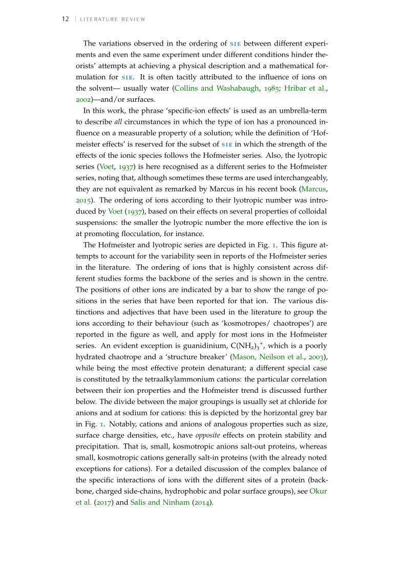
The variations observed in the ordering of sie between different experi-ments and even the same experiment under different conditions hinder the-orists’ attempts at achieving a physical description and a mathematical for-mulation for sie. It is often tacitly attributed to the influence of ions onthe solvent— usually water (Collins and Washabaugh, 1985; Hribar et al.,2002)—and/or surfaces.
In this work, the phrase ‘specific-ion effects’ is used as an umbrella-termto describe all circumstances in which the type of ion has a pronounced in-fluence on a measurable property of a solution; while the definition of ‘Hof-meister effects’ is reserved for the subset of sie in which the strength of theeffects of the ionic species follows the Hofmeister series. Also, the lyotropicseries (Voet, 1937) is here recognised as a different series to the Hofmeisterseries, noting that, although sometimes these terms are used interchangeably,they are not equivalent as remarked by Marcus in his recent book (Marcus,2015). The ordering of ions according to their lyotropic number was intro-duced by Voet (1937), based on their effects on several properties of colloidalsuspensions: the smaller the lyotropic number the more effective the ion isat promoting flocculation, for instance.
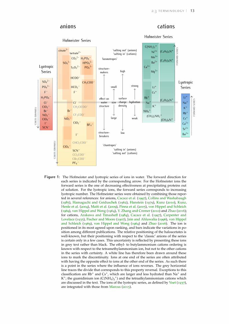
The Hofmeister and lyotropic series are depicted in Fig. 1. This figure at-tempts to account for the variability seen in reports of the Hofmeister seriesin the literature. The ordering of ions that is highly consistent across dif-ferent studies forms the backbone of the series and is shown in the centre.The positions of other ions are indicated by a bar to show the range of po-sitions in the series that have been reported for that ion. The various dis-tinctions and adjectives that have been used in the literature to group theions according to their behaviour (such as ‘kosmotropes/ chaotropes’) arereported in the figure as well, and apply for most ions in the Hofmeisterseries. An evident exception is guanidinium, C(NH2)3
+, which is a poorlyhydrated chaotrope and a ‘structure breaker’ (Mason, Neilson et al., 2003),while being the most effective protein denaturant; a different special caseis constituted by the tetraalkylammonium cations: the particular correlationbetween their ion properties and the Hofmeister trend is discussed furtherbelow. The divide between the major groupings is usually set at chloride foranions and at sodium for cations: this is depicted by the horizontal grey barin Fig. 1. Notably, cations and anions of analogous properties such as size,surface charge densities, etc., have opposite effects on protein stability andprecipitation. That is, small, kosmotropic anions salt-out proteins, whereassmall, kosmotropic cations generally salt-in proteins (with the already notedexceptions for cations). For a detailed discussion of the complex balance ofthe specific interactions of ions with the different sites of a protein (back-bone, charged side-chains, hydrophobic and polar surface groups), see Okuret al. (2017) and Salis and Ninham (2014).
2.3 terminology 13
Hofmeister Series Hofmeister Series
LyotropicSeries
LyotropicSeries
Cl–
F–HCO3 –
HCOO–CH3COO–
S2O32–
CO32–tartrate2–
PO43–
H2PO4 –HPO42–SO42–
citrate3–
CH2ClCOO–
CF3COO–Br–
ClO3 –NO3 –
BF4 –
I–
CHCl2COO–
SCN–ClO4 –
CCl3COO–CBr3COO–PF6 –
effect onwater
structuresize
surfacechargedensity
hydration
structure-makers
structure-breakers
small
large
high
low
strong
weak
‘kosmotropes’
‘salting out’ (anions)‘salting in’ (cations)
‘chaotropes’‘salting in’ (anions)
‘salting out’ (cations)
Na+Rb+
Cs+Li+
Mg2+
Ba2+Ca2+
Mn2+Ni2+
C(NH2)3+
K+
(CH3)2NH2+NH4+
(CH3)4N+
(C2H5)4N+
(C3H7)4N+
(C4H9)4N+
Cl–H2PO4 –
F–PO43–SO42–
ClO3 –Br–
NO3 –ClO4 –
I–SCN–
Na+
K+
Rb+
Cs+
Ca2+
Sr2+
Ba2+
Li+
anions cations
FORWARDSERIES
FORWARDSERIES
FORW
ARDS
ERIES
FORW
ARDS
ERIES
Figure 1: The Hofmeister and lyotropic series of ions in water. The forward direction foreach series is indicated by the corresponding arrow. For the Hofmeister ions theforward series is the one of decreasing effectiveness at precipitating proteins outof solution. For the lyotropic ions, the forward series corresponds to increasinglyotropic number. The Hofmeister series were obtained by combining those repor-ted in several references: for anions, Cacace et al. (1997), Collins and Washabaugh(1985), Hamaguchi and Geiduschek (1962), Hanstein (1979), Kunz (2010), Kunz,Henle et al. (2004), Maiti et al. (2009), Pinna et al. (2005), von Hippel and Schleich(1969), von Hippel and Wong (1964), Y. Zhang and Cremer (2010) and Zhao (2016);for cations, Arakawa and Timasheff (1984), Cacace et al. (1997), Carpenter andLovelace (1935), Fischer and Moore (1907), Jain and Ahluwalia (1996), von Hippeland Schleich (1969), von Hippel and Wong (1964) and Zhao (2016). The ion ispositioned in its most agreed upon ranking, and bars indicate the variations in po-sition among different publications. The relative positioning of the haloacetates iswell-known, but their positioning with respect to the ‘classic’ anions of the seriesis certain only in a few cases. This uncertainty is reflected by presenting these ionsin grey text rather than black. The ethyl- to butylammonium cations ordering isknown with respect to the tetramethylammonium ion, but not to the other cationsin the series with certainty. A white line has therefore been drawn around theseions to mark the discontinuity. Ions at one end of the series are often attributedwith having the opposite effect to ions at the other end of the series. As such thereis a point in the series where the influence of ions reverses. The grey horizontalline traces the divide that corresponds to this property reversal. Exceptions to thisclassification are Rb+ and Cs+, which are larger and less hydrated than Na+ andK+; the guanidinium ion (C(NH2)3
+) and the tetraalkylammonium cations whichare discussed in the text. The ions of the lyotropic series, as defined by Voet (1937),are integrated with those from Marcus (2015).
14 literature review
The salting-out ability of the tetraalkylammonium series decreases from(CH3)4N+, generally a salting-out cation (although this can change depend-ing on conditions, see Jain and Ahluwalia (1996) and von Hippel and Wong,1964), to (C4H9)4N+, which is a very effective salting-in agent (Jain andAhluwalia, 1996; Mason, Dempsey et al., 2009). This behaviour is analogousto the anions series, where smaller ions are more effective salting-out agents.But the water structure-making ability of the tetraalkylammonium cationsalso progressively increases with the length of the alkyl chains (and thereforethe cation size), due to ‘hydrophobic hydration’ (Marcus, 1994; Zhao, 2016),in contrast to what happens for the inorganic anions and cations. Therefore,the relationship between the size (and surface charge density) of the tetraal-kylammonium cations and their effect on water structure (and on proteinstability) is the opposite of the one observed for inorganic cations. Few ac-counts of the relative positioning of the tetraethyl- to tetrabutylammoniumions with respect to the main cations of the series are available: these ionsare therefore separated by a white line in Fig. 1, but their positioning followstheir general behaviour (Marcus, 1994; Zhao, 2016): (C2H5)4N+ is consideredas neutral to salting-in, and (C4H9)4N+ is extremely salting-in; (CH3)4N+ hasgenerally a salting-out effect, and can be more or less potent than NH4
+ de-pending on the experiment (Hyde et al., 2017).
The ordering of ions in the Hofmeister and lyotropic series is similar, butit is not identical. They are most similar for anions. Notable are the in-versions of fluoride with dihydrogenphosphate, chlorate with bromide, andnitrate and iodide with perchlorate between the series. For cations, the twoseries run in opposite directions, and whereas the divalent cations orderingis mirrored from the Hofmeister to the lyotropic series, the ordering of thealkali metal cations is not: the lyotropic series follows the cation size fromcaesium to lithium, whereas the Hofmeister series (in its most commonlyproposed order) runs as: potassium > sodium > rubidium > caesium > lith-ium. Notably, the lyotropic numbers are not available for the tetraalkylam-monium cations, and therefore these ions cannot be positioned within thelyotropic series. These distinctions between the Hofmeister and the lyotropicseries will be used later in the identification of sie trends in non-aqueoussolvents.
The lyotropic numbers are mostly determined by considering the stabil-ity of colloidal systems, whereas the Hofmeister series describes a muchbroader range of complex phenomena seen across biological systems, col-loidal dispersions, surface properties and solution structure. As noted byVoet, the lyotropic series correlates quite well with a single property of theions, their enthalpy of hydration, at least for the cations. The Hofmeisterseries does not correlate directly with a single property of the ions, and thisis because of the complex interplay of the properties of the ion, the inter-action of ion and solvent and, in the case of an interfacial interaction, thecharacteristics of the interface. Such complexity is one of the reasons why a

2.4 characteristics of non-aqueous solvents 15
theory of Hofmeister effects has not been achieved after more than a centuryfrom its first report.
In the ensuing chapters, we are going to also encounter cases where theordering is ion-dependent, but neither the Hofmeister nor lyotropic series isevident, as for anions, the viscosity B-coefficients (see Bη) (vbc) (Bilanicováet al., 2008; Collins and Washabaugh, 1985), the limiting molar ionic conduct-ivity (lmc) (Marcus, 2015), and for the ion pairing of tetraalkylammoniumsalts in ethanol (Giesecke, Mériguet et al., 2015).
In the cases where the series runs opposite to the conventional order, thathave been known as either the reverse, inverse or indirect Hofmeister series,the term ‘reverse’ is employed here.
The great success of the Hofmeister series is that it is so regularly observedin systems that are very different: a great many systems adhere to the Hof-meister paradigm (Kabalnov et al., 1995; Lagi et al., 2007; Lonetti et al., 2005;Oncsik et al., 2015; Piculell and Nilsson, 1989; Roberts et al., 2002; Ru et al.,2000; Salomäki et al., 2004; Schott, 1995; Vrbka et al., 2004; Washabaugh andCollins, 1986; Wiggins, 1997). The negative consequence of this is that, onoccasion, observations of sie are described as Hofmeister effects when thestrength of the influence of the ions does not follow the Hofmeister series,this somewhat clouds the field.
2.4 characteristics of non-aqueous solventsNon-aqueous solvents are liquids other than water. This work is concernedwith the subset of non-aqueous solvents that are capable of dissolving salts.These solvents usually have high dielectric constant in order to be able to sep-arate the charges of the electrolyte. But many other subtle and interwovencharacteristics come into play to define what is a good solvent for electro-lytes: the capability of donating/accepting hydrogen bonding, the physicalsize of the solvent molecules, the specific chemical groups in the solvent mo-lecule that interact with the anion and the cation. Extensive descriptions areavailable in Izutsu (2009) and Marcus (2015).
Table 2 lists the properties of the solvents included in this thesis. Amongthose, the empirical parameters expressing solvent acidity and basicity (do-nor and acceptors numbers) need illustration.
The Gutmann Donor Number DN is a measure of the basicity of a solvent.It represents the ability of solvent molecules to donate a free electron pairfrom their donor atoms (O, N or S). It is quantified as the negative of thestandard molar enthalpy of reaction −∆H−◦ of the solvent with the Lewisacid antimony pentachloride SbCl5, in dilute solution in the inert solvent1,2-dichloroethane at 25 ◦C (Marcus, 2015). These values are expressed inkcalmol−1 units, as a difference from the reference solvent 1,2-dichloroetha-ne, for which DN is set to 0.
16literaturereview
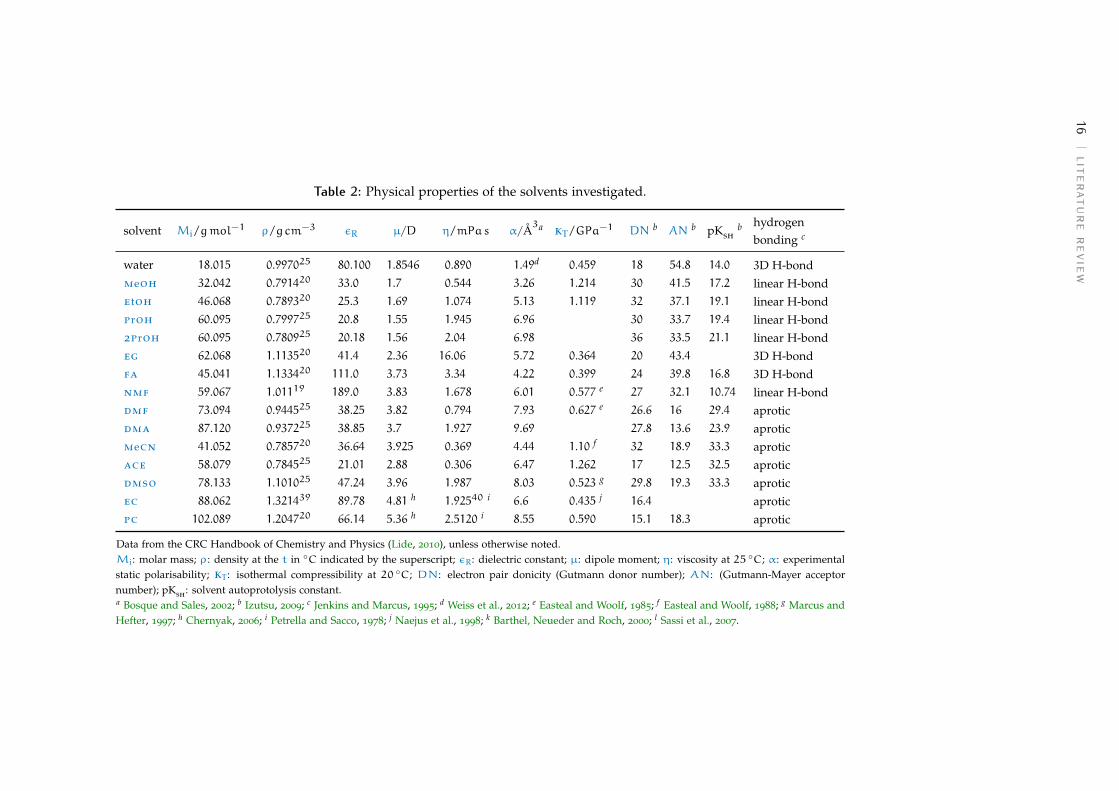
Table 2: Physical properties of the solvents investigated.
solvent Mi/gmol−1 ρ/g cm−3 εR µ/D η/mPas α/Å3a kT/GPa−1 DN b AN b pKsh
b hydrogenbonding c
water 18.015 0.997025 80.100 1.8546 0.890 1.49d 0.459 18 54.8 14.0 3D H-bondmeoh 32.042 0.791420 33.0 1.7 0.544 3.26 1.214 30 41.5 17.2 linear H-bondetoh 46.068 0.789320 25.3 1.69 1.074 5.13 1.119 32 37.1 19.1 linear H-bondproh 60.095 0.799725 20.8 1.55 1.945 6.96 30 33.7 19.4 linear H-bond2proh 60.095 0.780925 20.18 1.56 2.04 6.98 36 33.5 21.1 linear H-bondeg 62.068 1.113520 41.4 2.36 16.06 5.72 0.364 20 43.4 3D H-bondfa 45.041 1.133420 111.0 3.73 3.34 4.22 0.399 24 39.8 16.8 3D H-bondnmf 59.067 1.01119 189.0 3.83 1.678 6.01 0.577 e 27 32.1 10.74 linear H-bonddmf 73.094 0.944525 38.25 3.82 0.794 7.93 0.627 e 26.6 16 29.4 aproticdma 87.120 0.937225 38.85 3.7 1.927 9.69 27.8 13.6 23.9 aproticmecn 41.052 0.785720 36.64 3.925 0.369 4.44 1.10 f 32 18.9 33.3 aproticace 58.079 0.784525 21.01 2.88 0.306 6.47 1.262 17 12.5 32.5 aproticdmso 78.133 1.101025 47.24 3.96 1.987 8.03 0.523 g 29.8 19.3 33.3 aproticec 88.062 1.321439 89.78 4.81 h 1.92540 i 6.6 0.435 j 16.4 aproticpc 102.089 1.204720 66.14 5.36 h 2.5120 i 8.55 0.590 15.1 18.3 aprotic
Data from the CRC Handbook of Chemistry and Physics (Lide, 2010), unless otherwise noted.Mi: molar mass; ρ: density at the t in ◦C indicated by the superscript; εR: dielectric constant; µ: dipole moment; η: viscosity at 25 ◦C; α: experimentalstatic polarisability; kT: isothermal compressibility at 20 ◦C; DN: electron pair donicity (Gutmann donor number); AN: (Gutmann-Mayer acceptornumber); pKsh: solvent autoprotolysis constant.a Bosque and Sales, 2002; b Izutsu, 2009; c Jenkins and Marcus, 1995; d Weiss et al., 2012; e Easteal and Woolf, 1985; f Easteal and Woolf, 1988; g Marcus andHefter, 1997; h Chernyak, 2006; i Petrella and Sacco, 1978; j Naejus et al., 1998; k Barthel, Neueder and Roch, 2000; l Sassi et al., 2007.

2.5 methodology 17
The hydrogen bond donicity and electron pair acceptance of a solvent iscorrelated to its capability to contribute protons for hydrogen bonding. It istherefore limited to protic and protogenic solvents (solvents with a methylgroup adjacent to a C –– O, C ––– N, or NO2 group). The Gutmann–Mayer ac-ceptor numbers AN of a solvent (Lewis acid) are evaluated from the nuclearmagnetic resonance (nmr) chemical shift of the 31P atom of triethylphos-phine oxide Et3P –– O in dilute solution in the solvent of interest. The ANvalues are dimensionless numbers, the higher the number, the higher thesolvent acidity (Marcus, 2015).
Other scales have been defined, such as the solvent acidity scales areKosower’s Z values, Dimroth and Reichardt’s ET scale, Kamlet and Taft’sαKT parameter. conversely, solvent basicity scales include Kamlet and Taft’sβKT parameter (Izutsu, 2009).
The combination of properties of these solvents is very diverse. Based onthe combinations of some of the properties general classifications have beenintroduced (Izutsu, 2009), which are not adopted here.
2.5 methodologyIn the ensuing sections, a range of studies into sie in non-aqueous solventsare presented, grouped by solvent, and the sie trends that emerge are dis-cussed. It is immediately apparent that sie are as ubiquitous in non-aqueoussolvents as they are in water.
For each study the observed trend of sie for the cations and anions hasbeen extracted and displayed in a colour-coded table to assist in the inter-pretation of the data. The order of each table column runs from largestvalue at the top to smallest at the bottom. The series are compared to thosedefined in Fig. 1. A pale yellow cell background indicates a forward Hof-meister series, orange a reverse Hofmeister series, lilac a lyotropic series andpurple a reverse lyotropic series. No colour is used where a series does notfollow either the Hofmeister or lyotropic series. Where an individual ionis not included in the colour scheme for a particular series, this indicatesthat this ion is not in its correct location in the series. In some columns, theammonium cation and the tetraalkylammonium cations (NH4
+, (CH3)4N+,(C2H5)4N+, (C3H7)4N+, (C4H9)4N+), which I will collectively refer to as the‘ammonium class’ in the discussion, are offset to the right, so that they maybe easily considered separately from the alkali metal cations. This has beendone as these two classes of cations show consistent behaviour when con-sidered separately but not an overall trend when considered together.
The trends in sie observed for a range of properties of aqueous electrolytesolutions are shown in Table 3. These include (Marcus, 2015):

18 literature review
Table 3: Trends in sie observed in water. Data from Marcus (2015).
watermrt rdd* mhc lmc vbc
cations
Li+ Li+ (C4H9)4N+ Rb+ (C4H9)4N+
Na+ Na+ (C3H7)4N+ Cs+ (C3H7)4N+
K+ (C4H9)4N+ (C2H5)4N+ NH4+ (C2H5)4N+
NH4+ (CH3)4N+ K+ Li+
Li+ Na+ (CH3)4N+
Na+ (CH3)4N+ Na+
K+ Li+ NH4+
Rb+ (C2H5)4N+ K+
Cs+ (C3H7)4N+ Rb+
(C4H9)4N+ Cs+
anions
F– ClO4– SCN– = ClO4
– SO42 – HPO4
2 –
SO42 – I– F– CO3
2 – H2PO4–
Cl– Br– I– Br– CO32 –
Br– Cl– Cl– Cl– CH3COO–
NO3– Br– I– SO4
2 –
I– NO3– F–
ClO4– Cl–
SCN– SCN–
HPO42 – Br–
F– NO3–
HCOO– HCOO–
CH3COO– ClO4–
H2PO4– I–
* from electrolytes, ionic values not available.
• The nmr molecular reorientation time (mrt) of the solvent in the pres-ence of ions, calculated as the ratio τs(i) or/τs or, of the molecular reori-entation time constant in the presence of ions to the time constant ofthe neat solvent.
• The relative limiting static dielectric decrement (rdd) of an ion solu-tion as its concentration approaches zero, calculated as the ratio of thelimiting static dielectric decrement caused by the ion to the relative per-mittivity of the pure solvent −δ(i)/εs (ce → 0), with units dm3mol−1.
• The constant pressure standard partial molar heat capacity of the ion(mhc), C∞
pi in J K−1mol−1 which is the difference between the specificheat of the solution of the ion and that of the pure solvent, in the limitof infinite dilution.
• The limiting molar ionic conductivity (lmc) λ∞i (S cm2mol−1).
• The viscosity B-coefficients (see Bη) (vbc) of the Jones-Dole viscosityequation (Jones and Dole, 1929).
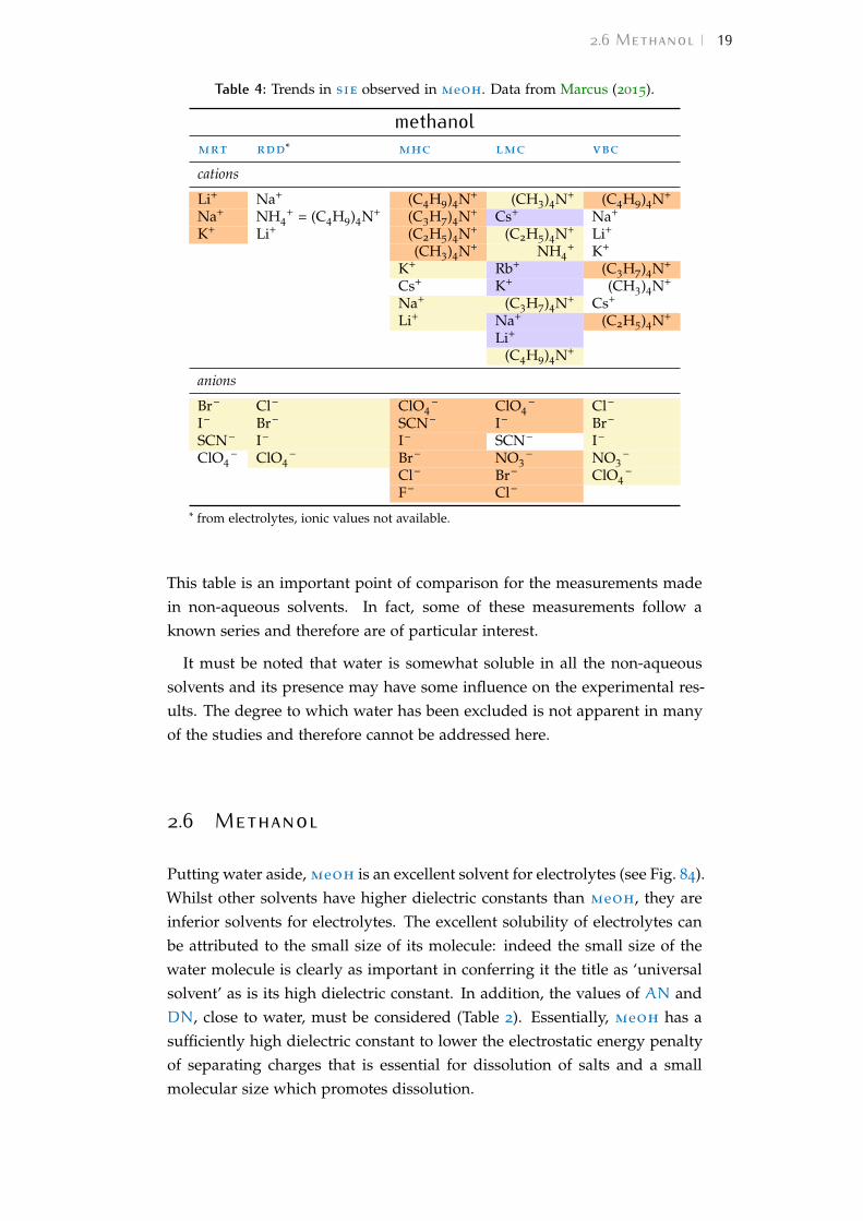
2.6 Methanol 19
Table 4: Trends in sie observed in meoh. Data from Marcus (2015).
methanolmrt rdd* mhc lmc vbc
cations
Li+ Na+ (C4H9)4N+ (CH3)4N+ (C4H9)4N+
Na+ NH4+ = (C4H9)4N+ (C3H7)4N+ Cs+ Na+
K+ Li+ (C2H5)4N+ (C2H5)4N+ Li+
(CH3)4N+ NH4+ K+
K+ Rb+ (C3H7)4N+
Cs+ K+ (CH3)4N+
Na+ (C3H7)4N+ Cs+
Li+ Na+ (C2H5)4N+
Li+
(C4H9)4N+
anions
Br– Cl– ClO4– ClO4
– Cl–
I– Br– SCN– I– Br–
SCN– I– I– SCN– I–
ClO4– ClO4
– Br– NO3– NO3
–
Cl– Br– ClO4–
F– Cl–
* from electrolytes, ionic values not available.
This table is an important point of comparison for the measurements madein non-aqueous solvents. In fact, some of these measurements follow aknown series and therefore are of particular interest.
It must be noted that water is somewhat soluble in all the non-aqueoussolvents and its presence may have some influence on the experimental res-ults. The degree to which water has been excluded is not apparent in manyof the studies and therefore cannot be addressed here.
2.6 MethanolPutting water aside, meoh is an excellent solvent for electrolytes (see Fig. 84).Whilst other solvents have higher dielectric constants than meoh, they areinferior solvents for electrolytes. The excellent solubility of electrolytes canbe attributed to the small size of its molecule: indeed the small size of thewater molecule is clearly as important in conferring it the title as ‘universalsolvent’ as is its high dielectric constant. In addition, the values of AN andDN, close to water, must be considered (Table 2). Essentially, meoh has asufficiently high dielectric constant to lower the electrostatic energy penaltyof separating charges that is essential for dissolution of salts and a smallmolecular size which promotes dissolution.
20 literature review
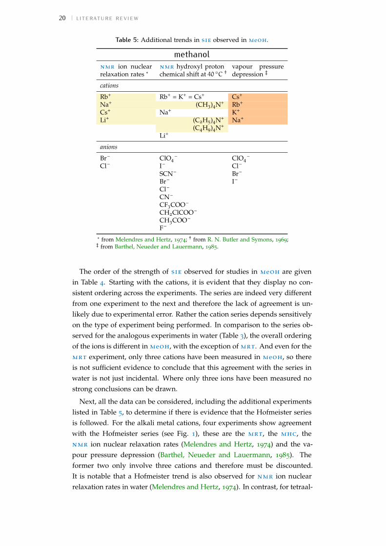
Table 5: Additional trends in sie observed in meoh.
methanolnmr ion nuclearrelaxation rates *
nmr hydroxyl protonchemical shift at 40 ◦C †
vapour pressuredepression ‡
cations
Rb+ Rb+ = K+ = Cs+ Cs+
Na+ (CH3)4N+ Rb+
Cs+ Na+ K+
Li+ (C2H5)4N+ Na+
(C4H9)4N+
Li+
anions
Br– ClO4– ClO4
–
Cl– I– Cl–
SCN– Br–
Br– I–
Cl–
CN–
CF3COO–
CH2ClCOO–
CH3COO–
F–
* from Melendres and Hertz, 1974; † from R. N. Butler and Symons, 1969;‡ from Barthel, Neueder and Lauermann, 1985.
The order of the strength of sie observed for studies in meoh are givenin Table 4. Starting with the cations, it is evident that they display no con-sistent ordering across the experiments. The series are indeed very differentfrom one experiment to the next and therefore the lack of agreement is un-likely due to experimental error. Rather the cation series depends sensitivelyon the type of experiment being performed. In comparison to the series ob-served for the analogous experiments in water (Table 3), the overall orderingof the ions is different in meoh, with the exception of mrt. And even for themrt experiment, only three cations have been measured in meoh, so thereis not sufficient evidence to conclude that this agreement with the series inwater is not just incidental. Where only three ions have been measured nostrong conclusions can be drawn.
Next, all the data can be considered, including the additional experimentslisted in Table 5, to determine if there is evidence that the Hofmeister seriesis followed. For the alkali metal cations, four experiments show agreementwith the Hofmeister series (see Fig. 1), these are the mrt, the mhc, thenmr ion nuclear relaxation rates (Melendres and Hertz, 1974) and the va-pour pressure depression (Barthel, Neueder and Lauermann, 1985). Theformer two only involve three cations and therefore must be discounted.It is notable that a Hofmeister trend is also observed for nmr ion nuclearrelaxation rates in water (Melendres and Hertz, 1974). In contrast, for tetraal-

2.7 Formamide 21
Table 6: Trends in sie observed in fa. Data from Marcus (2015).
formamidemrt rdd* lmc vbc
cations
Na+ (C4H9)4N+ NH4+ (C4H9)4N+
K+ Na+ Cs+ Na+
Rb+ Li+ (CH3)4N+ Li+
Cs+ Rb+ Rb+
K+ K+
(C2H5)4N+ (C2H5)4N+
Na+ Cs+
Li+ NH4+
(C3H7)4N+ (CH3)4N+
(C4H9)4N+
anions
Cl– NO3– NO3
–
Br– SCN– = Cl– = Br– Cl–
I– I– Br–
ClO4– I–
CH3COO– SCN–
* from electrolytes, ionic values not available.
kylammonium cations, the mhc shows a reversed Hofmeister series, whichis also observed in water. Lmc follows a lyotropic series for the alkali metalions both in water and meoh, and a forward Hofmeister series for the am-monium cations. The ordering of the latter group of cations is consistentalso between the vbc experiments in water and meoh, corresponding to areverse Hofmeister series.
Examining the anions, an altogether different situation emerges. Firstly, itis clear that there is a more consistent general order of the anions across theexperiments. Moreover, the anions are often ordered in accordance with theHofmeister series (or present only slight deviations from it), noting that insome cases it is in the reverse order. Significantly for mhc the Hofmeisterseries is followed in meoh but not in water. Clearly sie in meoh are oftenassociated with the Hofmeister series, perhaps moreso than for water.
2.7 FormamideFa, like water, is protic and forms a three-dimensional hydrogen bondednetwork, and therefore makes a particularly interesting comparison whenconsidering sie, where the hydrogen bonding network is often counted asplaying a determining role. The order of the strength of sie observed forstudies in fa are given in Table 6.
22 literature review
In considering the cations it is apparent that no consistent ordering of thecation series across the experiments is observed. For alkali metal cations,the lmc, vbc and mrt measurements yield results that are inconsistentwith the Hofmeister series. The alkali metal cations show a lyotropic serieswith regards to lmc (and mrt). The rdd follows a sie ordering whichis neither Hofmeister nor lyotropic, but it must be noted that the orderingof cations is the inverse of the ordering seen in water. In comparing thelmc measurements between water and fa, the overall cation trend is not inagreement. But if the ammonium class of cations (shown offset to the rightin the table) is considered separately to the alkali metal ions, both of thetrends considered separately are in good agreement.
When considering the anions, it is apparent that the ordering of the ionsobtained from conductivity studies is not consistent with the Hofmeisterseries. However the ordering obtained from vbc and mrt measurementsfollows the Hofmeister series, although the nitrate ion is not appropriatelyplaced in the vbc data and the mrt data only includes three ions. Manyexperiments do find a single ion misplaced in the series yet the overall effectis still generally considered as a Hofmeister series, so that precedent is fol-lowed here as well. It must be noted that vbc does not follow the Hofmeisterseries in water.
Overall it can be concluded that both the cations and the anions showsome evidence of sie consistent with those seen in aqueous systems.
2.8 N -methylformamideN-methylformamide (nmf) is a highly polar, water miscible organic solventwith applications in chemistry and biology. The experimental data showingthe trends in the strength of the sie for nmf is presented in Table 7.
No consistent trend in the cation series is observed across a range of ex-periments. For some experiments there is a suggestion that the Hofmeisterseries for cations is followed, but there is an insufficient number of ions meas-ured to make a strong case for this. Interestingly, the forward Hofmeisterordering of cations in rdd coincides with the one observed in fa (Table 6),and is the reverse of the trend seen in water. More often occurring is thelyotropic series for alkali metal cations. The lmc of alkali metals cationsfollows a lyotropic series, whereas the ammonium class of cations followsa forward Hofmeister series: both trends taken separately agree with thoseof the same property in water. Notably for the vbc experiments the oddsituation occurs, in which the ammonium cations have the same order asthey do in water, whereas the alkali metal ions show a trend that is the exactreverse (lyotropic) of that seen in water (reverse lyotropic).

2.9 N ,N -dimethylformamide 23
Table 7: Trends in sie observed in nmf. Data from Marcus (2015).
N-methylformamidemrt rdd* mhc lmc vbc
cations
Li+ (C4H9)4N+ K+ (CH3)4N+ (C3H7)4N+
Na+ Na+ Cs+ (C2H5)4N+ (C2H5)4N+
K+ Li+ Na+ NH4+ Cs+
Rb+ Li+ Cs+ K+
Cs+ Rb+ Na+
K+ Li+
Na+ (CH3)4N+
(C3H7)4N+ NH4+
(C4H9)4N+
Li+
anions
Cl– = Br– I– SCN– Cl–
I– Br– I– Br–
Cl– Br– I–
ClO4–
Cl–
* from electrolytes, ionic values not available.
There is scarce data to consider for the anions in nmf. In this case the lmcshows a different trend to that seen in water and neither are Hofmeister like.The remaining experimental data suggests a correlation with the Hofmeisterseries for mrt and vbc and a reverse Hofmeister trend for mhc, albeit onan insufficient number of ions to draw the conclusion confidently.
2.9 N ,N -dimethylformamideN,N-dimethylformamide (dmf) is miscible with water and the majority oforganic solvents, as such it is used extensively as a solvent for chemicalreactions. A summary of the trends in the strength of the sie in dmf for arange of experiments is presented in Table 8.
No persistent trend is seen in the strength of sie for the cations or the an-ions in dmf. The ion-specific trends for alkali metal cations for mhc and thereduction of SO2, follow forward and reverse Hofmeister series respectively.When comparing the lmc trends in water and dmf we find that in bothsolvents the ammonium class of cations follows the Hofmeister series andthe other ions separately follow the lyotropic series, but the overall trend ex-hibited in the two solvents is different. The tetraalkylammonium cations inmhc (only two ions, therefore the identification is not strongly supported)and vbc follow a reverse Hofmeister series as in water, but the alkali metalstrend in mhc differs and corresponds to a forward Hofmeister rather than
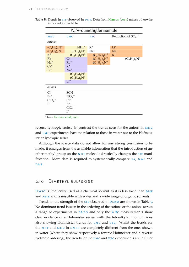
24 literature review
Table 8: Trends in sie observed in dmf. Data from Marcus (2015) unless otherwiseindicated in the table.
N,N-dimethylformamidemhc lmc vbc Reduction of SO2 *
cations
(C3H7)4N+ NH4+ K+ Li+
(C2H5)4N+ (CH3)4N+ Na+ Na+
K+ (C2H5)4N+ (C4H9)4N+ K+
Rb+ Cs+ (C3H7)4N+ (C2H5)4N+
Na+ Rb+ (C2H5)4N+
Cs+ K+
Li+ Na+
(C3H7)4N+
(C4H9)4N+
Li+
anions
Cl– SCN–
Br– NO3–
ClO4– Cl–
I– Br–
ClO4–
I–
* from Gardner et al., 1981.
reverse lyotropic series. In contrast the trends seen for the anions in mhcand lmc experiments have no relation to those in water nor to the Hofmeis-ter or lyotropic series.
Although the scarce data do not allow for any strong conclusion to bemade, it emerges from the available information that the introduction of an-other methyl group on the nmf molecule drastically changes the sie mani-festation. More data is required to systematically compare fa, nmf anddmf.
2.10 Dimethyl sulfoxideDmso is frequently used as a chemical solvent as it is less toxic than dmfand nmf and is miscible with water and a wide range of organic solvents.
Trends in the strength of the sie observed in dmso are shown in Table 9.No dominant trend is seen in the ordering of the cations or the anions acrossa range of experiments in dmso and only the mhc measurements showclear evidence of a Hofmeister series, with the tetraalkylammonium ionsalso showing Hofmeister trends for lmc and vbc. Whilst the trends forthe mrt and mhc in dmso are completely different from the ones shownin water (where they show respectively a reverse Hofmeister and a reverselyotropic ordering), the trends for the lmc and vbc experiments are in fuller

2.11 additional solvents 25
Table 9: Trends in sie observed in dmso. Data from Marcus (2015).
dimethyl sulfoxidemrt mhc lmc vbc
cations
Na+ Na+ (CH3)4N+ (C4H9)4N+
K+ K+ (C2H5)4N+ Li+
Rb+ Cs+ Cs+ (C3H7)4N+
Cs+ Li+ Rb+ K+
K+ Na+
Na+ Rb+
Li+ Cs+
(C4H9)4N+ (C2H5)4N+
(CH3)4N+
anions
Br– I– ClO4– Br–
I– ClO4– SCN– I–
Br– NO3– NO3
–
F– Br– Cl–
Cl– I– SCN–
Cl– ClO4–
agreement with water when the tetraalkylammonium ions and alkali metalsare considered independently. Note that this differs from the correlationseen for vbc measurements in nmf, in which the alkali metal cations werein the reverse order.
The little data available for the anions show no consistent ordering, norecognisable series, or analogy with the trends in water.
2.11 additional solvents
In this section, the data for the solvents etoh, pc and ethylene carbonate(1,3-dioxolan-2-one) (ec) are presented and discussed. As these solventsdo not dissolve a wide range of electrolytes, the information is necessarilylimited.
Other solvents, for which even less information is available, are not dis-cussed in detail, but the series observed in these solvents are included inthe summarising Table 13 to give a picture as comprehensive as possible.These solvents consist of the protic 1-propanol (propan-1-ol) (proh), ethyl-ene glycol (ethane-1,2-diol) (eg), nitromethane (meno2) and the aprotic acet-one (propan-2-one) (ace) and mecn.

26 literature review
Table 10: Trends in sie observed in etoh. Data from Marcus (2015).
ethanolmhc lmc vbc
cations
(C4H9)4N+ (CH3)4N+ Na+
(C3H7)4N+ (C2H5)4N+ (C4H9)4N+
(C2H5)4N+ Cs+ (C3H7)4N+
K+ Rb+ Li+
Cs+ K+ K+
Na+ (C3H7)4N+ Rb+
Li+ NH4+ (C2H5)4N+
Na+ Cs+
(C4H9)4N+ (CH3)4N+
Li+
anions
I– ClO4– Br–
Br– SCN– ClO4–
Cl– I–
F– NO3–
Br–
CH3COO–
Cl–
2.11.1 Ethanol
The sie observed in experiments using etoh as a solvent are summarisedin Table 10. Considering the cations first, there is no consistent trend in thestrength of sie exhibited across the experiments, although there is a majorityof cases where the Hofmeister series appears.
Mhc data for the alkali metal cations display the same ordering as indmso, nmf and dmf, and they differ from water in the alkali metals seriesordering. In etoh the lmc data for the alkali metal cations follows alyotropic series which is consistent with the ordering obtained in water,whereas a reverse lyotropic series is seen for alkali metal ions in the vbcdata, which is in agreement with water as well. Consistency is also observedfor the tetraalkylammonium cations between water and etoh in lmc (notethat NH4
+ does not follow the series in etoh) and vbc. The lmc and vbctrends therefore agree in water for the ammonium ions and the alkali metalions considered separately, as already observed for other solvents.
For the anions, the conductivity and mhc data is consistent with the Hof-meister series but inconsistent with the trend obtained in water. That is, thelmc and mhc data in etoh shows a reverse Hofmeister series for the anionsthat is not observed in those measurements in water.
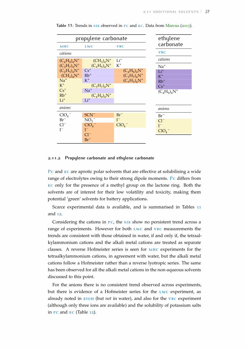
2.11 additional solvents 27
Table 11: Trends in sie observed in pc and ec. Data from Marcus (2015).
propylene carbonatemhc lmc vbc
cations
(C4H9)4N+ (CH3)4N+ Li+
(C3H7)4N+ (C2H5)4N+ K+
(C2H5)4N+ Cs+ (C4H9)4N+
(CH3)4N+ Rb+ (C3H7)4N+
Na+ K+ (C2H5)4N+
K+ (C3H7)4N+
Cs+ Na+
Rb+ (C4H9)4N+
Li+ Li+
anions
ClO4– SCN– Br–
Br– NO3– I–
Cl– ClO4– ClO4
–
I– I–
Cl–
Br–
ethylenecarbonatevbc
cations
Na+
Li+
K+
Rb+
Cs+
(C4H9)4N+
anions
Br–
Cl–
I–
ClO4–
2.11.2 Propylene carbonate and ethylene carbonate
Pc and ec are aprotic polar solvents that are effective at solubilising a widerange of electrolytes owing to their strong dipole moments. Pc differs fromec only for the presence of a methyl group on the lactone ring. Both thesolvents are of interest for their low volatility and toxicity, making thempotential ‘green’ solvents for battery applications.
Scarce experimental data is available, and is summarised in Tables 11and 12.
Considering the cations in pc, the sie show no persistent trend across arange of experiments. However for both lmc and vbc measurements thetrends are consistent with those obtained in water, if and only if, the tetraal-kylammonium cations and the alkali metal cations are treated as separateclasses. A reverse Hofmeister series is seen for mhc experiments for thetetraalkylammonium cations, in agreement with water, but the alkali metalcations follow a Hofmeister rather than a reverse lyotropic series. The samehas been observed for all the alkali metal cations in the non-aqueous solventsdiscussed to this point.
For the anions there is no consistent trend observed across experiments,but there is evidence of a Hofmeister series for the lmc experiment, asalready noted in etoh (but not in water), and also for the vbc experiment(although only three ions are available) and the solubility of potassium saltsin pc and ec (Table 12).

28 literature review
Table 12: Additional trends in sie observed for pc and ec.
propylene carbonatesolubility of K+
salts *ft-ir intensity ofC –– O stretchingband *
anions
SCN– Cl–
I– SCN–
ClO4– Br–
Br– I–
CNO– ClO4–
Cl– CNO–
F–
ethylenecarbonatesolubility of K+
salts †
anions
I–
ClO4–
NO3–
Br–
Cl–
F–
* from Peruzzi, Lo Nostro et al., 2015; † from Peruzzi, Ninham et al., 2012.
The cation data in ec are only available for one experiment, vbc, whichshows a reverse lyotropic ordering of alkali metal ion, in accordance to theobserved series in water and other solvents. Anion effects in ec show in-stead Hofmeister ordering, that agrees with the pc ordering for both theexperiments available.
Ec solvates mainly through ion-dipole interactions, which are stronger forsmall anions, therefore dispersion forces must contribute to the solubility ofelectrolytes in a significant way.
2.12 other investigationsExperiments in eg and fa show that sie do not follow the Hofmeister series.The Diels-Alder reaction performed in these solvents in the presence of urea,guanidinium, perchlorate, chloride and quaternary ammonium salts showsa very different salt-dependence than when performed in water (Breslowand Guo, 1988).
Despite these results it is clear that both the Hofmeister series and thelyotropic series are evident in a wide range of solvents and that neither canbe considered to be unique to water. Consistent with this are the experimentsof Bilanicová et al. (2008), who studied the effects of different anions on theactivity of the Pseudomonas cepacia lipase in 2-methyl-2-butanol. The enzymewas obtained by lyophilising a concentrated salt solution in water, at pH 7,and it was then dissolved in 2-methyl-2-butanol. The activity of the enzymewas the highest in a completely dry medium (reaction carried in the presenceof molecular sieves), and the activity follows a Hofmeister series: SO4
2 – >H2PO4
– /HPO42 – > Cl– > Br– = I– = SCN– .
2.12 other investigations 29
Investigations of sie were performed also in liquid chromatography ex-periments. Smuts et al. (2014) used a cyclofructan-6-based chiral stationaryphase doped with barium to resolve chiral phosphoric and sulfonic acids.The effect of the counterion of the barium salt added to the mobile phaseon retention and enantioselectivity was investigated. It was found that theyincrease in the order CH3COO– < methanesulfonate (msa-) < CF3COO–
< ClO4– , which is in agreement with the Hofmeister series. They also com-
pared the selectivity and retention by changing the mobile phase from meohto etoh. They found that the latter offers higher retention and improves en-antioselectivity. They explain the phenomenon with the fact that the lowerdielectric constant of etoh forces closer ion pairs with the barium cation ad-sorbed on the stationary phase, which causes a longer retention and closerinteraction with the chiral stationary phase. Sanganyado et al. (2014) in-vestigated the effect of Hofmeister anions on the enantioresolution, enan-tioselectivity and retention factor of basic chiral pharmaceuticals in polarionic mode liquid chromatography. Retention follows the ion-specific series:CH3COO– > HCOO– > NO3
– .An ion specific non-Hofmeister series is observed for the kinetics of the
reaction of iodination of acetone (Lo Nostro, Mazzini et al., 2016), followingthe trend HBr < HCl < HClO4 < HF < H2SO4 < H3PO4.
A technique that has been recently introduced for studying ion associationin solution is electrophoretic nmr. The study of the association of mono-valent Hofmeister anions paired with the (CH3)4N+ cation in the deuteratedsolvents D2O, dmso, mecn, meoh, etoh, shows complex ion-specificitythat does not follow the Hofmeister or lyotropic series. These series and arestrongly solvent-dependent (Giesecke, Mériguet et al., 2015). Complex non-Hofmeister series are also encountered for the cation association with dis-perse polyethylene oxide in meoh solution (Giesecke, Hallberg et al., 2016).The authors identify that ion-polymer binding only happens for cations witha surface charge density below 0.10Å
−2to 0.15Å
−2. Interestingly, no relev-
ant changes in the series are observed for different cation-counterion pair-ings (the counterions investigated are AcO– , I– and ClO4
– ) have been in-vestigated as counterions. This is in disagreement to the lmwa principle,which is extensively reviewed later in Section 4.4.

30 literature review
2.13 an overall view
The sie trends across a range of experiments for a range of solvents aresummarised in Table 13. This table also includes the data for solvents thathave not been discussed in the previous sections because of the little amountof data available: proh, eg, meno2, ace and mecn.
Whilst in some cases the data is limited, the survey reveals some inter-esting information. The sie observed are different for different solvents. Itwould be desirable to relate the sie to the properties of the solvent, how-ever at this stage the complexity and extensive variation seen in sie across arange of solvents and a range of experiments does not allow for simple gen-eralisations. Additionally, in many experiments the confidence with whichthe sie can be labelled as a Hofmeister series or a lyotropic series is dimin-ished due to the limited availability of data.
The lmc and vbc experiments are particularly interesting as the datais the most extensive across the range of solvents for these experiments. Incomparing the trends observed in the non-aqueous solvents to those in water,it is apparent that the ammonium cations should be treated separately tothe alkali metal cations, as in no case did the overall ordering of the ionscoincide between water and a non-aqueous solvent, but in many cases theordering did coincide when the classes were treated separately. Consideringthe lmc of cations, in general the ammonium class of cations follows theHofmeister series and the alkali metal cations follow the lyotropic series.It should be highlighted here that the lyotropic numbers are not availablefor the ammonium class of cations, therefore the ordering of these ions canonly be identified as either ‘Hofmeister series’ or ‘other’. For the anions,a reverse Hofmeister series is observed when a series is evident, but notin all cases. It is expected that the lmc will be strongly influenced by thesize and solvation of an ion and for this reason the tetraalkylammoniumcations might be expected to behave differently to other ions because oftheir size (i.e. the increase in size due to the addition of methyl groups inthe four lateral chains is not compensated by the change in solvation orother properties of the ion, as discussed in Section 2.3). As with the lmcexperiments, the vbc experiments show agreements with both the sub-seriesof cations. The vbc experiments reveal that the cations follow the sametrends as in water for both of the series considered separately for etoh, dmf(two ions only), dmso, pc (two ions) and ec. However, for three solvent, thevbc ordering of the ammonium cations agrees with that in water, whereasthe ordering of the alkali metal cations does not: in meoh and fa, the alkalimetal cations follow a different trend (other than a lyotropic or Hofmeisterseries), and for nmf, the alkali metal cations series is reversed compared

2.13 an overall view 31
Table 13: Summary of the sie series seen for a range of experiments in water andnon-aqueous solvents. Protic solvents are in bold, aprotic solvents are it-alicised. Series with three or less ions have been indicated in parentheses.
cationssolvent mrt rdd mhc lmc vbc
R4N+† M+‡ R4N+ M+ R4N+ M+
water R-HS other R-HS R-lyo HS lyo R-HS R-lyomeoh R-HS (3) other R-HS HS HS lyo R-HS (3) otheretoh / / R-HS HS HS lyo R-HS R-lyofa R-lyo other§ / / HS lyo R-HS (3) othernmf R-lyo other§ / HS (3) HS lyo R-HS lyodmf / / ? (2) R-HS HS HS lyo R-HS / (2)dmso R-lyo / / HS HS (3) lyo R-HS R-lyopc / / R-HS HS HS lyo R-HS / (2)ec / / / / / / / R-lyo
proh / / R-HS / (2) HS lyo / /eg R-lyo / / / HS lyo / /meno2 / / / R-lyo HS lyo / /ace / / / / HS lyo R-HS / (2)mecn / / ? (2) R-HS other HS lyo R-HS other
anionssolvent mrt rdd mhc lmc vbc
water HS R-HS other other othermeoh HS (3) HS R-HS R-HS HSetoh / / R-HS R-HS / (2)fa HS (3) / / other HSnmf HS (3) / R-HS (3) other HS (3)dmf / / other other /dmso / (2) / other other otherpc / / other R-HS HS (3)ec / / / / HS (3)
proh / / R-HS R-HS /eg HS (3) / / HS /meno2 / / other R-HS /ace / / / other othermecn / / HS R-HS HS
† ammonium cations, where R=H, (CH3), (C2H5), (C3H7) or (C4H9).‡ alkali metals.§ reverse series of the one in water for rdd.

32 literature review
to that in water. That is, in nmf the forward lyotropic series is observed,whereas the reverse lyotropic series is observed in water. Nmf and fa alsoshow reversed sie series with respect to water in the rdd experiment. Thecause of series reversal in water has attracted some interest and has beenrelated to salt concentration and surface charge (Parsons, Boström, Maceinaet al., 2010). This investigation reveals that the solvent itself can also causeseries reversal. It remains an interesting and important challenge to explainthese phenomena.
A similar situation exists for the mhc data: the ammonium cations con-sistently follow a reverse Hofmeister ordering across solvents, but the al-kali metal cations show a lyotropic trend only in water and meno2, and bycontrast the rest of the non-aqueous solvents follows a forward Hofmeisterseries.
For anions, the ordering observed in water is seldom reflected by the non-aqueous solvents. It is very interesting that both in the lmc and vbc case,a wider agreement of series is seen for cations rather than anions. Thishighlights that, with respect to those properties, the solvents behave simil-arly with cations and less so with anions. One might expect the opposite asstronger sie are usually observed for anions.
2.14 summaryThere is evidence of the Hofmeister series (forward or reverse) for the anionsin all solvents except dmf, dmso, meno2 and ace and for the cations inall solvents apart from ec. Though it is notable that the Hofmeister seriesis not uniformly observed for a particular experiment across the solventsand no particular effect of the solvent being protic is evident. Notably, inmeoh the anions follow the Hofmeister series in the mhc, lmc and vbcexperiments even though this is not the case for these experiments in water.Also the other non-aqueous solvents can show a Hofmeister series in one ofthese experiments, where it has not been observed in water. Whereas forthe cations, Hofmeister or lyotropic series are evident in a number of exper-iments with good consistency across solvents. Clearly the situation is verycomplex, and explanations for this situation are difficult to find. However,recognition that these series exist in non-aqueous solvents brings into focusthe depth of complexity of sie evident when a wider range of solvents areobserved and highlights that there is a substantial degree of similarity in siepresent across a range of solvents, albeit with some outstanding differences.
The available evidence indicates that all solvents on occasion will exhibitthe Hofmeister series and the lyotropic series and no particular property ofa solvent can be correlated to the Hofmeister effect or the lyotropic series.

2.14 summary 33
Therefore, we can conclude that neither series can be attributed to the prop-erties of a solvent. The significant challenge is then to determine why par-ticular experiments reveal the Hofmeister series or lyotropic series in onesolvent and not another solvent. Resolution of this may well require a deepunderstanding of the full range of sie. This question is addressed in thefollowing chapters.
It also emerges that, in order to achieve a comprehensive picture of thisphenomenon in non-aqueous solvents, many more experiments must be per-formed and theoretical investigations pursued. This is no small task andrequires a renewed interest in the fundamental and systematic investigationof the properties of non-aqueous electrolyte solutions. It is desirable that the-orists engaged in tackling the complexity of sie extend their considerationsto include non-aqueous solvents. I argue that explanations for sie in aque-ous systems can be rigorously tested by assessing their utility in explainingsie observed in other solvents.

3 E L E C T R O S T R I C T I O N
This chapter is reproduced with minor changes from:
V. Mazzini and V. S. J. Craig (2017), ‘What Is the Fundamental Ion-specificSeries for Anions and Cations? Ion Specificity in Standard Partial MolarVolumes of Electrolytes and Electrostriction in Water and Non-aqueous Sol-vents’, Chem. Sci. 8 (10 2017), pp. 7052–7065, doi: 10.1039/C7SC02691A.
3.1 motivationA major point of debate is the fundamental origin of sie, as highlightedin Section 1.5. The questions framing the debate are: What are the funda-mental interactions for the manifestation of sie? Do they originate fromthe ion alone, or the ion-solvent interaction, or the ion-ion interaction (i.e.at higher ion concentrations), or the ion-surface interaction, or a mix of theabove?
Here I attend to the above questions by investigating properties of a verysimple system, in the conviction that the ion-specificity (if present) manifes-ted in this setting is a close expression of the fundamental mechanisms. Thesimplest electrolyte solution setting can be individuated in an infinitely di-lute solution. Therein, only ion-solvent interactions can be assumed to takeplace, and ion- ion interactions are excluded. In addition, we can look at aproperty of the solution for which no interacting surfaces intervene: a bulkproperty. Therefore the interference of interacting surfaces is removed, andwe are left with a system where only ion-solvent interactions are in place.This is the best possible setting for studying the role of the solvent on sie,and also to gather information on whether sie are manifest in the limit ofinfinite dilution, and in the absence of surface or ion-ion interactions.
Finally, in order for this general investigation of solvent effects on sietrends to be meaningful, data must be available for a large number of sol-vents: the standard partial molar volume of electrolytes in solution and thederived electrostriction are properties that respond to all of the above re-quirements. They are available in the critically compiled collections by Mil-lero (1971, 1972a) for aqueous electrolytes and by Marcus and Hefter (2004)for electrolytes in non-aqueous solvents.
35

36 electrostriction
3.2 partial molar volumes and electrostrictionThe partial molar volume of a species ‘i’ in solution represents the changein volume of the solution upon addition of one mole of solute at constanttemperature, pressure, and other components of the solution (Lewis andRandall, 1961; Millero, 1972b):
V i =
(∂V
∂ni
)
T, P, nj 6= i
[1]
where V i is the partial molar volume of the solute in solution; V the totalvolume of the solution and ni the number of moles of solute present in solu-tion. The partial molar volume is an important quantity because it can bedemonstrated that the partial molar volumes of the components of a solutionare additive:
V =∑
i
niV i [2]
The partial molar electrostrictive volume of the species ‘i’ in solution (V i el),can be calculated in the following way (Marcus, 2011):
V i el = V i − V i intr [3]
Where V i is the experimentally derived partial molar volume of the species‘i’ in solution and V i intr is the intrinsic molar volume of the species ‘i’, whichis not directly measurable by experiment. If the standard partial molar volumeV−◦i is used in the calculation, the electrostrictive volume at infinite dilutionV−◦i el (also known as V∞
i el, standard partial molar electrostrictive volume) isobtained, which reflects only the interactions between the solute and thesolvent (and not solute-solute effects). These standard quantities are thesubject of the present chapter.
The dependence of the standard partial molar volume V−◦i on solvent prop-
erties has been investigated by Hamann and Lim (1954) in water and threeother solvents: there exists an inverse linear relationship between the stand-ard partial volume of the electrolytes and the compressibility of the solvent.Later, Marcus, Hefter and Pang (1994) applied a stepwise multivariable lin-ear least-squares regression to the standard partial molar volumes of ions insolution in order to relate them to solvent and ion properties. They foundthat the cube of the ion radius is the major contributor to the standard par-tial molar volume in solution. Secondly, the electron pair-sharing capabilityof the ion plays a role. The solvent compressibility and self-association arealso found to play a role, but no correlation is observed with solvent di-pole moment and relative permittivity. Marcus has also investigated the

3.2 partial molar volumes and electrostriction 37
ion specificity of electrostriction (Marcus, 2013): he analysed the correlationbetween the standard molar ionic electrostriction and the surface tension in-crement generated by ions. He found a reasonable correlation for cationsbut not for anions.
The connection between sie and partial standard molar volumes of ions insolution can be made in two ways. Jenkins and Marcus (1995) demonstratethat a relationship between the viscosity B-coefficient of the Jones-Dole equa-tion and the molar volume of the ion in solution exists. On the other hand,the ion specificity of the viscosity B-coefficient has been known for a longtime, starting with the work of Cox and Wolfenden (1934). Additionally Col-lins (1997) accommodated it intrinsically in the formulation of his ‘lmwa’.This suggests that the link between electrostriction, which derives from thestandard molar volumes of electrolytes, and sie is straightforward. If sucha connection can be elaborated in non-aqueous solvents, additional insightinto the nature of sie will be gained, as partial molar volumes are useful forthe understanding of the interactions occurring in aqueous and non-aqueoussolutions (Millero, 1972b). The standard molar quantities are therefore per-fectly suited for the purpose of studying sie in non-aqueous solvents.
Much careful work has been done in the experimental determination ofpartial molal volumes of electrolytes in solution, therefore abundant inform-ation is already available in the literature, and has been extensively reviewed(Marcus and Hefter, 2004; Millero, 1971). As the experimental observableused for the calculation of the electrostrictive volume is the density of thesolution, this type of experiment can be quite simple to perform in orderto acquire data where missing (given the right experimental apparatus isavailable — see Appendix G.1.1). Attempts to calculate electrostriction theor-etically have also been made (Desnoyers et al., 1965; Kasprowicz and Kielich,1967; Marcus and Hefter, 1999; Padova, 1963).
The electrolyte exerts a constricting pressure on the order of hundreds ofMPa on the surrounding solvent molecules (Marcus, 2011), thus reducingthe volume the solvent occupies. Figure 2 shows the dependence of the elec-trostrictive volume on molal concentration in water (calculated using thedensity data of electrolyte solutions from Söhnel and Novotný, 1985): itsmagnitude is different for each electrolyte. The electrostriction is larger atsmall concentrations as the effect saturates when all of the solvent is elec-trostricted.
As electrostriction happens when a salt is dissolved in a solvent, thevolume of the resulting solution is usually different from the sum of thevolumes of the individual components, and generally smaller. This phe-nomenon is attributed to the fact that, under the huge electric field exertedby an ion, the solvent contracts (or more rarely expands). This results inthe partial molar volume of the electrolyte being different from the ‘intrinsic’
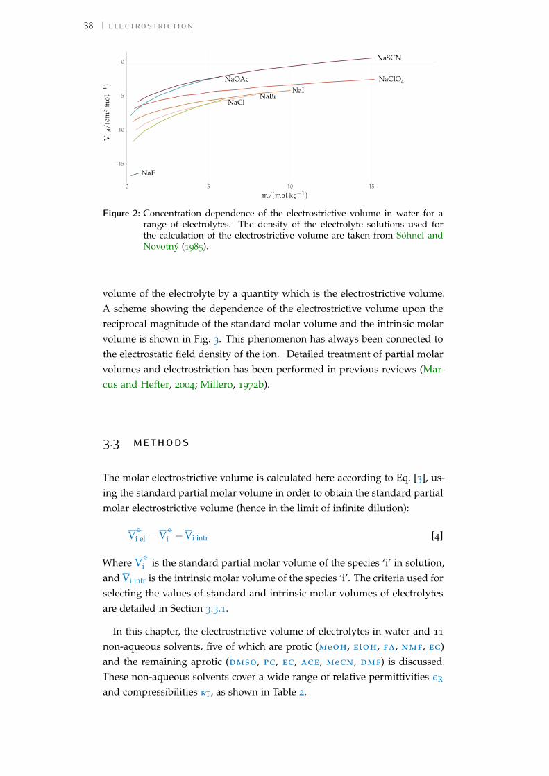
38 electrostriction
NaBrNaCl
NaClO4
NaF
NaI
NaOAc
NaSCN
−15
−10
−5
0
0 5 10 15
m/(molkg−1)
Vie
l/(cm
3mol−
1)
Figure 2: Concentration dependence of the electrostrictive volume in water for arange of electrolytes. The density of the electrolyte solutions used forthe calculation of the electrostrictive volume are taken from Söhnel andNovotný (1985).
volume of the electrolyte by a quantity which is the electrostrictive volume.A scheme showing the dependence of the electrostrictive volume upon thereciprocal magnitude of the standard molar volume and the intrinsic molarvolume is shown in Fig. 3. This phenomenon has always been connected tothe electrostatic field density of the ion. Detailed treatment of partial molarvolumes and electrostriction has been performed in previous reviews (Mar-cus and Hefter, 2004; Millero, 1972b).
3.3 methodsThe molar electrostrictive volume is calculated here according to Eq. [3], us-ing the standard partial molar volume in order to obtain the standard partialmolar electrostrictive volume (hence in the limit of infinite dilution):
V−◦i el = V
−◦i − V i intr [4]
Where V−◦i is the standard partial molar volume of the species ‘i’ in solution,
and V i intr is the intrinsic molar volume of the species ‘i’. The criteria used forselecting the values of standard and intrinsic molar volumes of electrolytesare detailed in Section 3.3.1.
In this chapter, the electrostrictive volume of electrolytes in water and 11non-aqueous solvents, five of which are protic (meoh, etoh, fa, nmf, eg)and the remaining aprotic (dmso, pc, ec, ace, mecn, dmf) is discussed.These non-aqueous solvents cover a wide range of relative permittivities εR
and compressibilities kT, as shown in Table 2.

3.3 methods 39
solvent
saltV i intr
solution
V i
solution
V i
solution
V i
solution
V i
beforemixing
idealI.
V i el = 0
V i ≡ V i intr
strictionV i el < 0
V i < V i intr
V i > 0 V i < 0
II. III.expansion
IV.
V i el > 0
V i > V i intr
Figure 3: Schematic of the range of possible outcomes for the final solution volumewhen a salt is dissolved in a solvent, depending on the effect of elec-trostriction. In this picture, the depicted volume of salt corresponds toone mole (therefore it represents the intrinsic molar volume). This pictureparticularly helps in visualising the case where the molar volume of thesalt in solution is negative.
Electrolytes containing the following monovalent anions and cations areconsidered in this chapter (here listed according to the Hofmeister series):
AcO− > F− > Cl− > Br− > I− > ClO4− > SCN−
K+ > Na+ > Rb+ > Cs+ > Li+
Where AcO– stands for the acetate anion, CH3COO– . It must be noted thatfor this set of anions, the difference between Hofmeister and lyotropic seriesis only reflected in the position of I– and ClO4
– . Conversely, the ordering ofthe cations is very different in the two series (see Fig. 1).
3.3.1 Data sources and selection criteria
This section details the criteria used for selecting the values to analyse andto employ in Eq. [4].
The values of the standard molar volumes, V−◦i , are taken from Millero’s
review (Millero, 1971) in the case of water (with the exception of SCN– , forwhich the conventional volume indicated by Marcus (Table 2, 2011) has beenused), and from Marcus and Hefter’s review (Marcus and Hefter, 2004) inthe case of non-aqueous solvents. Not all the V
−◦i values of electrolytes in
non-aqueous solvents have been experimentally determined (and reviewed),but, using an extra-thermodynamic assumption, Marcus and Hefter (2004)calculated the V
−◦i values of the single ions in solution, which are additive.
The missing values (where possible) have therefore been calculated by usingthe ionic standard partial molar volumes. These values are affected by a sig-
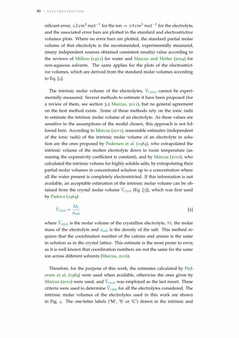
40 electrostriction
nificant error, ±2 cm3mol−1 for the ion⇒±4 cm3mol−1 for the electrolyte,and the associated error bars are plotted in the standard and electrostrictivevolumes plots. Where no error bars are plotted, the standard partial molarvolume of that electrolyte is the recommended, experimentally measured,(many independent sources obtained consistent results) value according tothe reviews of Millero (1971) for water and Marcus and Hefter (2004) fornon-aqueous solvents. The same applies for the plots of the electrostrict-ive volumes, which are derived from the standard molar volumes accordingto Eq. [4].
The intrinsic molar volume of the electrolytes, V i intr, cannot be experi-mentally measured. Several methods to estimate it have been proposed (fora review of them, see section 3.2 Marcus, 2011), but no general agreementon the best method exists. Some of these methods rely on the ionic radiito estimate the intrinsic molar volume of an electrolyte. As these values aresensitive to the assumptions of the model chosen, this approach is not fol-lowed here. According to Marcus (2011), reasonable estimates (independentof the ionic radii) of the intrinsic molar volume of an electrolyte in solu-tion are the ones proposed by Pedersen et al. (1984), who extrapolated theintrinsic volume of the molten electrolyte down to room temperature (as-suming the expansivity coefficient is constant), and by Marcus (2010), whocalculated the intrinsic volume for highly soluble salts, by extrapolating theirpartial molar volumes in concentrated solution up to a concentration whereall the water present is completely electrostricted. If this information is notavailable, an acceptable estimation of the intrinsic molar volume can be ob-tained from the crystal molar volume Vcryst (Eq. [5]), which was first usedby Padova (1964):
Vcryst =Mi
ρsalt[5]
where Vcryst is the molar volume of the crystalline electrolyte, Mi the molarmass of the electrolyte and ρsalt is the density of the salt. This method re-quires that the coordination number of the cations and anions is the samein solution as in the crystal lattice. This estimate is the most prone to error,as it is well known that coordination numbers are not the same for the sameion across different solvents (Marcus, 2016).
Therefore, for the purpose of this work, the estimates calculated by Ped-ersen et al. (1984) were used when available, otherwise the ones given byMarcus (2010) were used, and Vcryst was employed as the last resort. Thesecriteria were used to determine V i intr for all the electrolytes considered. Theintrinsic molar volumes of the electrolytes used in this work are shownin Fig. 4. The one-letter labels (‘M’, ‘S’ or ‘C’) drawn in the intrinsic and
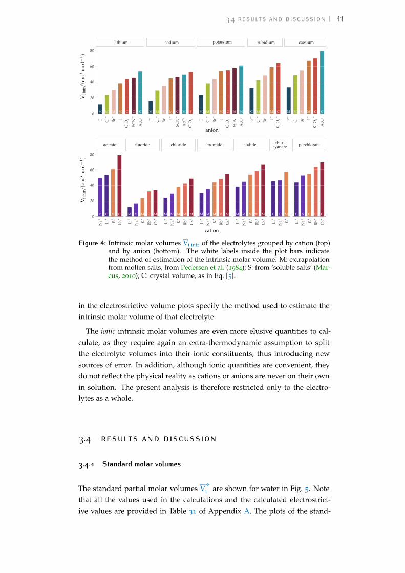
3.4 results and discussion 41
MM CM M CC MM SM M MC MM CM M MM MM CC M MM CM M C
lithium sodium potassium rubidium caesium
Br–
Cl–
ClO
4–
F– I–
AcO
–
SCN
–
Br–
Cl–
ClO
4–
F– I–
AcO
–
SCN
–
Br–
Cl–
ClO
4–
F– I–
AcO
–
SCN
–
Br–
Cl–
ClO
4–
F– I–
Br–
Cl–
ClO
4–
F– I–
AcO
–
0
20
40
60
80
anion
Vii
ntr/(cm
3mol−
1)
CMCM MMM M C MMM M M MMM M M MMM M M MC C CCC S C
acetate fluoride chloride bromide iodide thio-cyanate perchlorate
Cs+
K+
Li+
Na+
Cs+
K+
Li+
Na+
Rb+
Cs+
K+
Li+
Na+
Rb+
Cs+
K+
Li+
Na+
Rb+
Cs+
K+
Li+
Na+
Rb+
K+
Li+
Na+
Cs+
K+
Li+
Na+
Rb+
0
20
40
60
80
cation
Vii
ntr/(cm
3mol−
1)
Figure 4: Intrinsic molar volumes V i intr of the electrolytes grouped by cation (top)and by anion (bottom). The white labels inside the plot bars indicatethe method of estimation of the intrinsic molar volume. M: extrapolationfrom molten salts, from Pedersen et al. (1984); S: from ‘soluble salts’ (Mar-cus, 2010); C: crystal volume, as in Eq. [5].
in the electrostrictive volume plots specify the method used to estimate theintrinsic molar volume of that electrolyte.
The ionic intrinsic molar volumes are even more elusive quantities to cal-culate, as they require again an extra-thermodynamic assumption to splitthe electrolyte volumes into their ionic constituents, thus introducing newsources of error. In addition, although ionic quantities are convenient, theydo not reflect the physical reality as cations or anions are never on their ownin solution. The present analysis is therefore restricted only to the electro-lytes as a whole.
3.4 results and discussion3.4.1 Standard molar volumes
The standard partial molar volumes V−◦i are shown for water in Fig. 5. Note
that all the values used in the calculations and the calculated electrostrict-ive values are provided in Table 31 of Appendix A. The plots of the stand-
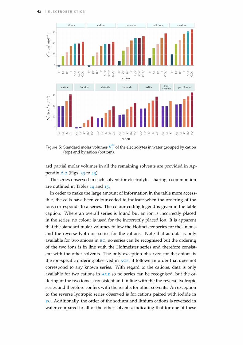
42 electrostriction
lithium sodium potassium rubidium caesium
Br–
Cl–
ClO
4–
F– I–
AcO
–
SCN
–
Br–
Cl–
ClO
4–
F– I–
AcO
–
SCN
–
Br–
Cl–
ClO
4–
F– I–
AcO
–
SCN
–
Br–
Cl–
ClO
4–
F– I–
Br–
Cl–
ClO
4–
F– I–
AcO
–
0
20
40
60
anion
V−◦ i/(cm
3mol−
1)
acetate fluoride chloride bromide iodide thio-cyanate perchlorate
Cs+
K+
Li+
Na+
Cs+
K+
Li+
Na+
Rb+
Cs+
K+
Li+
Na+
Rb+
Cs+
K+
Li+
Na+
Rb+
Cs+
K+
Li+
Na+
Rb+
K+
Li+
Na+
Cs+
K+
Li+
Na+
Rb+
0
20
40
60
cation
V−◦ i/(cm
3mol−
1)
Figure 5: Standard molar volumes V−◦i of the electrolytes in water grouped by cation
(top) and by anion (bottom).
ard partial molar volumes in all the remaining solvents are provided in Ap-pendix A.2 (Figs. 33 to 43).
The series observed in each solvent for electrolytes sharing a common ionare outlined in Tables 14 and 15.
In order to make the large amount of information in the table more access-ible, the cells have been colour-coded to indicate when the ordering of theions corresponds to a series. The colour coding legend is given in the tablecaption. Where an overall series is found but an ion is incorrectly placedin the series, no colour is used for the incorrectly placed ion. It is apparentthat the standard molar volumes follow the Hofmeister series for the anions,and the reverse lyotropic series for the cations. Note that as data is onlyavailable for two anions in ec, no series can be recognised but the orderingof the two ions is in line with the Hofmeister series and therefore consist-ent with the other solvents. The only exception observed for the anions isthe ion-specific ordering observed in ace: it follows an order that does notcorrespond to any known series. With regard to the cations, data is onlyavailable for two cations in ace so no series can be recognised, but the or-dering of the two ions is consistent and in line with the the reverse lyotropicseries and therefore confers with the results for other solvents. An exceptionto the reverse lyotropic series observed is for cations paired with iodide ineg. Additionally, the order of the sodium and lithium cations is reversed inwater compared to all of the other solvents, indicating that for one of these
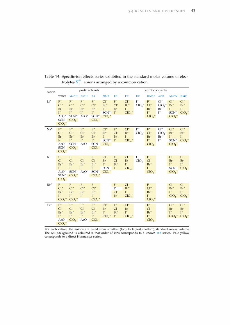
3.4 results and discussion 43
Table 14: Specific-ion effects series exhibited in the standard molar volume of elec-trolytes V
−◦i : anions arranged by a common cation.
cation protic solvents aprotic solvents
water meoh etoh fa nmf eg pc ec dmso ace mecn dmf
Li+ F– F– F– F– Cl– F– Cl– I– F– Cl– Cl– Cl–
Cl– Cl– Cl– Cl– Br– Cl– Br– ClO4– Cl– ClO4
– Br– Br–
Br– Br– Br– Br– I– Br– I– Br– Br– I– I–
I– I– I– I– SCN– I– ClO4– I– I– SCN– ClO4
–
AcO– SCN– AcO– SCN– ClO4– ClO4
– ClO4–
SCN– ClO4– ClO4
–
ClO4–
Na+ F– F– F– F– Cl– F– Cl– I– F– Cl– Cl– Cl–
Cl– Cl– Cl– Cl– Br– Cl– Br– ClO4– Cl– ClO4
– Br– Br–
Br– Br– Br– Br– I– Br– I– Br– Br– I– I–
I- I– I– I– SCN– I– ClO4– I– I– SCN– ClO4
–
AcO– SCN– AcO– SCN– ClO4– ClO4
– ClO4–
SCN– ClO4– ClO4
–
ClO4–
K+ F– F– F– F– Cl– F– Cl– I– F– Cl– Cl–
Cl– Cl– Cl– Cl– Br– Cl– Br– ClO4– Cl– Br– Br–
Br– Br– Br– Br– I– Br– I– Br– I– I–
I– I– I– I– SCN– I– ClO4– I– SCN– ClO4
–
AcO– SCN– AcO– SCN– ClO4– ClO4
– ClO4–
SCN– ClO4– ClO4
–
ClO4–
Rb+ F– F– F– F– F– Cl– F– Cl– Cl–
Cl– Cl– Cl– Cl– I– Br– Cl– Br– Br–
Br– Br– Br– Br– Cl– I– Br– I– I–
I– I– I– I– Br– ClO4– I– ClO4
– ClO4–
ClO4– ClO4
– ClO4– ClO4
–
Cs+ F– F– F– F– Cl– F– Cl– F– Cl– Cl–
Cl– Cl– Cl– Cl– Br– Cl– Br– Cl– Br– Br–
Br– Br– Br– Br– I– Br– I– Br– I– I–
I– I– I– I– ClO4– I– ClO4
– I– ClO4– ClO4
–
AcO– ClO4– AcO– ClO4
– ClO4–
ClO4–
For each cation, the anions are listed from smallest (top) to largest (bottom) standard molar volume.The cell background is coloured if that order of ions corresponds to a known sie series. Pale yellowcorresponds to a direct Hofmeister series.
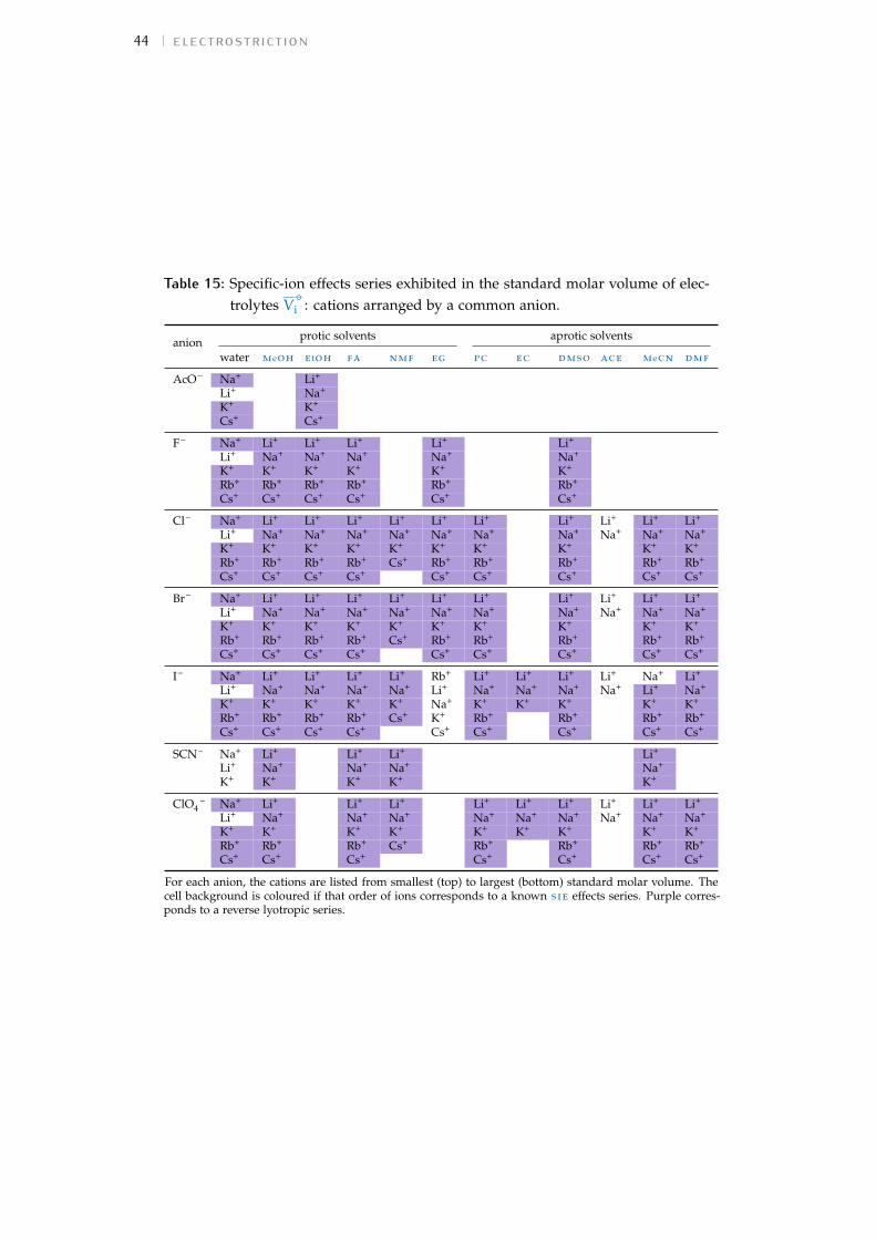
44 electrostriction
Table 15: Specific-ion effects series exhibited in the standard molar volume of elec-trolytes V
−◦i : cations arranged by a common anion.
anion protic solvents aprotic solvents
water meoh etoh fa nmf eg pc ec dmso ace mecn dmf
AcO– Na+ Li+
Li+ Na+
K+ K+
Cs+ Cs+
F– Na+ Li+ Li+ Li+ Li+ Li+
Li+ Na+ Na+ Na+ Na+ Na+
K+ K+ K+ K+ K+ K+
Rb+ Rb+ Rb+ Rb+ Rb+ Rb+
Cs+ Cs+ Cs+ Cs+ Cs+ Cs+
Cl– Na+ Li+ Li+ Li+ Li+ Li+ Li+ Li+ Li+ Li+ Li+
Li+ Na+ Na+ Na+ Na+ Na+ Na+ Na+ Na+ Na+ Na+
K+ K+ K+ K+ K+ K+ K+ K+ K+ K+
Rb+ Rb+ Rb+ Rb+ Cs+ Rb+ Rb+ Rb+ Rb+ Rb+
Cs+ Cs+ Cs+ Cs+ Cs+ Cs+ Cs+ Cs+ Cs+
Br– Na+ Li+ Li+ Li+ Li+ Li+ Li+ Li+ Li+ Li+ Li+
Li+ Na+ Na+ Na+ Na+ Na+ Na+ Na+ Na+ Na+ Na+
K+ K+ K+ K+ K+ K+ K+ K+ K+ K+
Rb+ Rb+ Rb+ Rb+ Cs+ Rb+ Rb+ Rb+ Rb+ Rb+
Cs+ Cs+ Cs+ Cs+ Cs+ Cs+ Cs+ Cs+ Cs+
I– Na+ Li+ Li+ Li+ Li+ Rb+ Li+ Li+ Li+ Li+ Na+ Li+
Li+ Na+ Na+ Na+ Na+ Li+ Na+ Na+ Na+ Na+ Li+ Na+
K+ K+ K+ K+ K+ Na+ K+ K+ K+ K+ K+
Rb+ Rb+ Rb+ Rb+ Cs+ K+ Rb+ Rb+ Rb+ Rb+
Cs+ Cs+ Cs+ Cs+ Cs+ Cs+ Cs+ Cs+ Cs+
SCN– Na+ Li+ Li+ Li+ Li+
Li+ Na+ Na+ Na+ Na+
K+ K+ K+ K+ K+
ClO4– Na+ Li+ Li+ Li+ Li+ Li+ Li+ Li+ Li+ Li+
Li+ Na+ Na+ Na+ Na+ Na+ Na+ Na+ Na+ Na+
K+ K+ K+ K+ K+ K+ K+ K+ K+
Rb+ Rb+ Rb+ Cs+ Rb+ Rb+ Rb+ Rb+
Cs+ Cs+ Cs+ Cs+ Cs+ Cs+ Cs+
For each anion, the cations are listed from smallest (top) to largest (bottom) standard molar volume. Thecell background is coloured if that order of ions corresponds to a known sie effects series. Purple corres-ponds to a reverse lyotropic series.
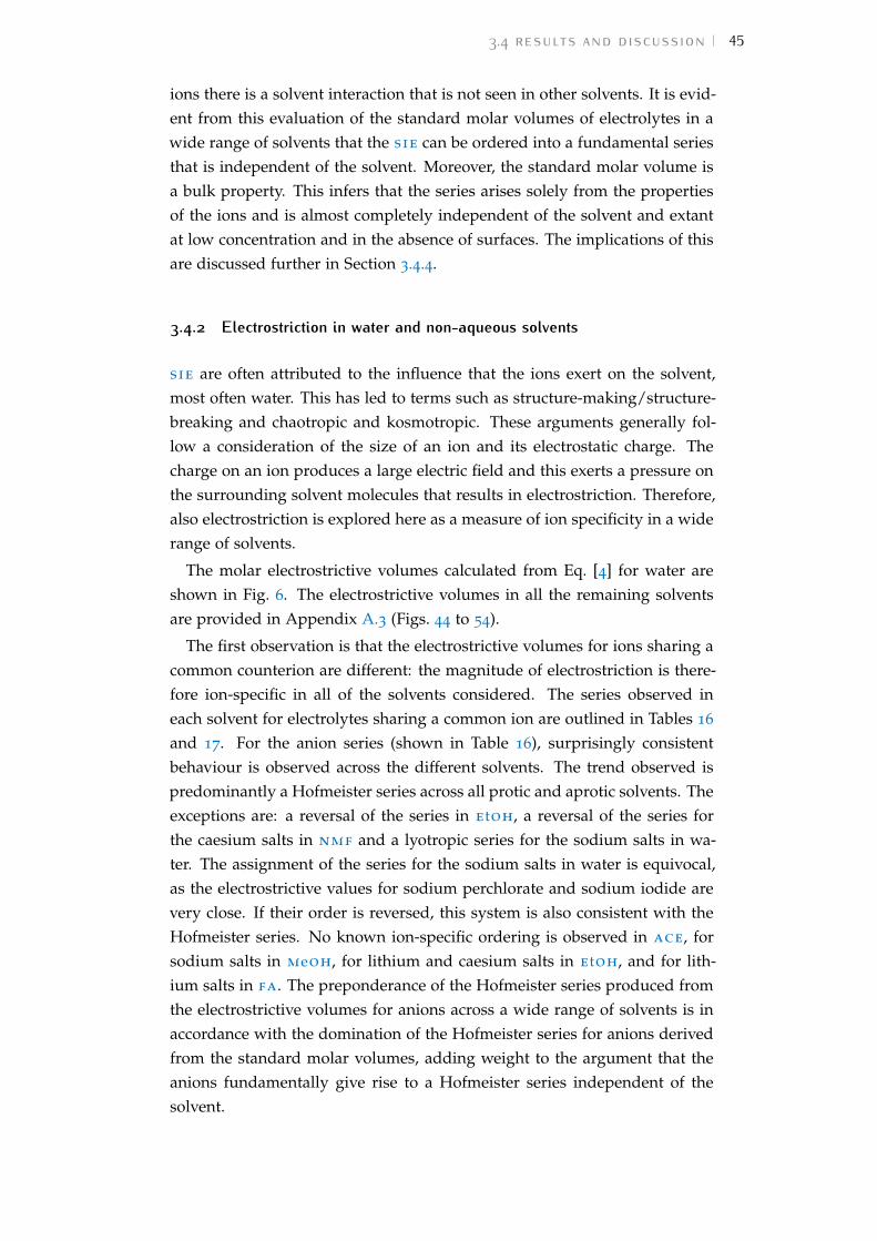
3.4 results and discussion 45
ions there is a solvent interaction that is not seen in other solvents. It is evid-ent from this evaluation of the standard molar volumes of electrolytes in awide range of solvents that the sie can be ordered into a fundamental seriesthat is independent of the solvent. Moreover, the standard molar volume isa bulk property. This infers that the series arises solely from the propertiesof the ions and is almost completely independent of the solvent and extantat low concentration and in the absence of surfaces. The implications of thisare discussed further in Section 3.4.4.
3.4.2 Electrostriction in water and non-aqueous solvents
sie are often attributed to the influence that the ions exert on the solvent,most often water. This has led to terms such as structure-making/structure-breaking and chaotropic and kosmotropic. These arguments generally fol-low a consideration of the size of an ion and its electrostatic charge. Thecharge on an ion produces a large electric field and this exerts a pressure onthe surrounding solvent molecules that results in electrostriction. Therefore,also electrostriction is explored here as a measure of ion specificity in a widerange of solvents.
The molar electrostrictive volumes calculated from Eq. [4] for water areshown in Fig. 6. The electrostrictive volumes in all the remaining solventsare provided in Appendix A.3 (Figs. 44 to 54).
The first observation is that the electrostrictive volumes for ions sharing acommon counterion are different: the magnitude of electrostriction is there-fore ion-specific in all of the solvents considered. The series observed ineach solvent for electrolytes sharing a common ion are outlined in Tables 16and 17. For the anion series (shown in Table 16), surprisingly consistentbehaviour is observed across the different solvents. The trend observed ispredominantly a Hofmeister series across all protic and aprotic solvents. Theexceptions are: a reversal of the series in etoh, a reversal of the series forthe caesium salts in nmf and a lyotropic series for the sodium salts in wa-ter. The assignment of the series for the sodium salts in water is equivocal,as the electrostrictive values for sodium perchlorate and sodium iodide arevery close. If their order is reversed, this system is also consistent with theHofmeister series. No known ion-specific ordering is observed in ace, forsodium salts in meoh, for lithium and caesium salts in etoh, and for lith-ium salts in fa. The preponderance of the Hofmeister series produced fromthe electrostrictive volumes for anions across a wide range of solvents is inaccordance with the domination of the Hofmeister series for anions derivedfrom the standard molar volumes, adding weight to the argument that theanions fundamentally give rise to a Hofmeister series independent of thesolvent.
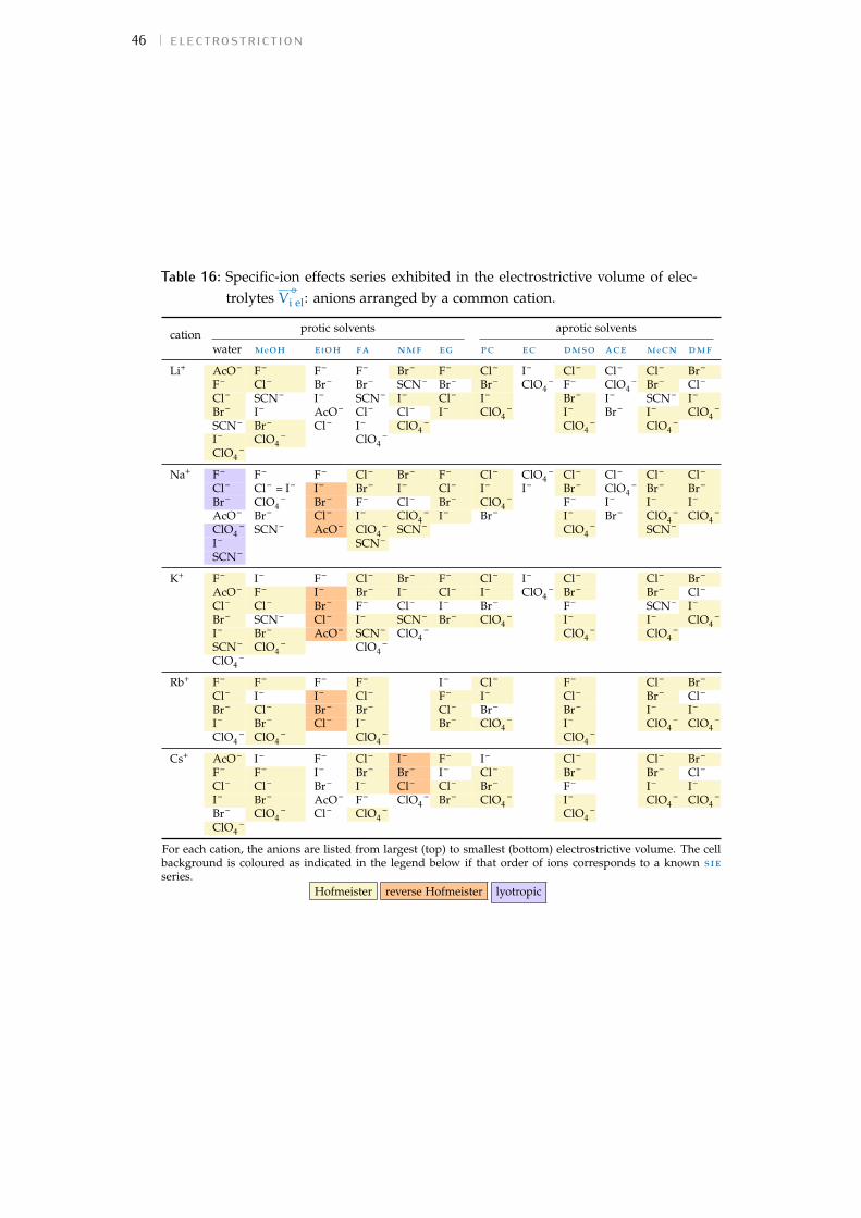
46 electrostriction
Table 16: Specific-ion effects series exhibited in the electrostrictive volume of elec-trolytes V
−◦i el: anions arranged by a common cation.
cation protic solvents aprotic solvents
water meoh etoh fa nmf eg pc ec dmso ace mecn dmf
Li+ AcO– F– F– F– Br– F– Cl– I– Cl– Cl– Cl– Br–
F– Cl– Br– Br– SCN– Br– Br– ClO4– F– ClO4
– Br– Cl–
Cl– SCN– I– SCN– I– Cl– I– Br– I– SCN– I–
Br– I– AcO– Cl– Cl– I– ClO4– I– Br– I– ClO4
–
SCN– Br– Cl– I– ClO4– ClO4
– ClO4–
I– ClO4– ClO4
–
ClO4–
Na+ F– F– F– Cl– Br– F– Cl– ClO4– Cl– Cl– Cl– Cl–
Cl– Cl– = I– I– Br– I– Cl– I– I– Br– ClO4– Br– Br–
Br– ClO4– Br– F– Cl– Br– ClO4
– F– I– I– I–
AcO– Br– Cl– I– ClO4– I– Br– I– Br– ClO4
– ClO4–
ClO4– SCN– AcO– ClO4
– SCN– ClO4– SCN–
I– SCN–
SCN–
K+ F– I– F– Cl– Br– F– Cl– I– Cl– Cl– Br–
AcO– F– I– Br– I– Cl– I– ClO4– Br– Br– Cl–
Cl– Cl– Br– F– Cl– I– Br– F– SCN– I–
Br– SCN– Cl– I– SCN– Br– ClO4– I– I– ClO4
–
I– Br– AcO– SCN– ClO4– ClO4
– ClO4–
SCN– ClO4– ClO4
–
ClO4–
Rb+ F– F– F– F– I– Cl– F– Cl– Br–
Cl– I– I– Cl– F– I– Cl– Br– Cl–
Br– Cl– Br– Br– Cl– Br– Br– I– I–
I– Br– Cl– I– Br– ClO4– I– ClO4
– ClO4–
ClO4– ClO4
– ClO4– ClO4
–
Cs+ AcO– I– F– Cl– I– F– I– Cl– Cl– Br–
F– F– I– Br– Br– I– Cl– Br– Br– Cl–
Cl– Cl– Br– I– Cl– Cl– Br– F– I– I–
I– Br– AcO– F– ClO4– Br– ClO4
– I– ClO4– ClO4
–
Br– ClO4– Cl– ClO4
– ClO4–
ClO4–
For each cation, the anions are listed from largest (top) to smallest (bottom) electrostrictive volume. The cellbackground is coloured as indicated in the legend below if that order of ions corresponds to a known sieseries.
Hofmeister reverse Hofmeister lyotropic

3.4 results and discussion 47
Table 17: Specific-ion effects series exhibited in the electrostrictive volume of elec-trolytes V
−◦i el: cations arranged by a common anion.
anion protic solvents aprotic solvents
water meoh etoh fa nmf eg pc ec dmso ace mecn dmf
AcO– Cs+ Li+
Li+ Cs+
K+ K+
Na+ Na+
F– Rb+ Rb+ Li+ Rb+ Rb+ Rb+
Na+ Na+ Rb+ Na+ Li+ Li+
K+ Cs+ Na+ Li+ Na+ Na+
Li+ Li+ K+ K+ K+ K+
Cs+ K+ Cs+ Cs+ Cs+ Cs+
Cl– Na+ Na+ Li+ Na+ Cs+ Na+ Li+ Li+ Li+ Rb+ Rb+
K+ Rb+ Na+ Cs+ K+ K+ Cs+ K+ Na+ Cs+ K+
Rb+ K+ K+ K+ Na+ Li+ Na+ Na+ K+ Cs+
Cs+ Cs+ Rb+ Rb+ Li+ Rb+ Rb+ Cs+ Na+ Na+
Li+ Li+ Cs+ Li+ Cs+ K+ Rb+ Li+ Li+
Br– Na+ Na+ Li+ Na+ Li+ Li+ Li+ Li+ Li+ Rb+ Li+
K+ Rb+ Na+ Cs+ Cs+ Na+ Cs+ Na+ Na+ Cs+ Rb+
Rb+ K+ K+ Rb+ K+ K+ Rb+ K+ K+ K+
Cs+ Cs+ Rb+ Li+ Na+ Rb+ Na+ Rb+ Na+ Cs+
Li+ Li+ Cs+ K+ Cs+ K+ Cs+ Li+ Na+
I– Na+ Cs+ Li+ Cs+ Cs+ Rb+ Cs+ K+ Cs+ Li+ Rb+ Cs+
Cs+ Na+ Na+ Na+ K+ K+ Rb+ Li+ K+ Na+ Na+ Rb+
K+ Rb+ K+ Rb+ Na+ Na+ K+ Na+ Li+ Cs+ K+
Rb+ K+ Rb+ K+ Li+ Li+ Li+ Na+ K+ Na+
Li+ Li+ Cs+ Li+ Cs+ Na+ Rb+ Li+ Li+
SCN– K+ K+ Li+ Li+ K+
Na+ Na+ K+ K+ Li+
Li+ Li+ Na+ Na+ Na+
ClO4– Na+ Na+ Na+ Na+ Na+ Na+ Na+ Li+ Na+ Na+
Rb+ Rb+ Cs+ Cs+ Cs+ Li+ Cs+ Na+ Rb+ Rb+
Cs+ Cs+ Rb+ Li+ Rb+ K+ Li+ Cs+ Cs+
K+ K+ Li+ K+ Li+ Rb+ K+ Li+
Li+ Li+ K+ K+ K+ Li+ K+
For each anion, the cations are listed from largest (top) to smallest (bottom) electrostrictive volume. Thecell background is coloured as indicated in the legend below if that order of ions corresponds to a knownsie series.
Hofmeister reverse Hofmeister lyotropic reverse lyotropic
new series 1 reverse new series 1 new series 2
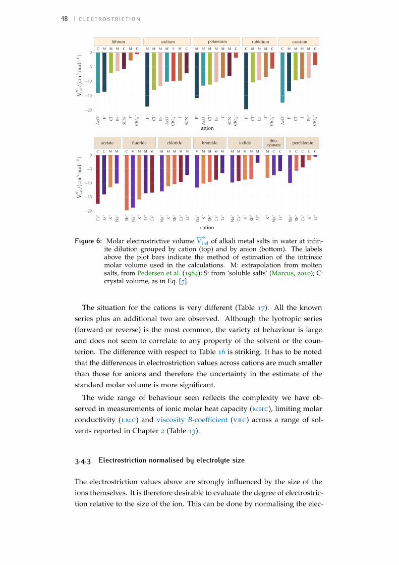
48 electrostriction
MM CM MC C MM SM MM C MM CM MM M MM CC M MM CM MC
lithium sodium potassium rubidium caesium
Br–
Cl–
ClO
4–
F– I–
AcO
–
SCN
–
Br–
Cl–
ClO
4–
F– I–
AcO
–
SCN
–
Br–
Cl–
ClO
4–
F– I–
AcO
–
SCN
–
Br–
Cl–
ClO
4–
F– I–
Br–
Cl–
ClO
4–
F– I–
AcO
–
−20
−15
−10
−5
0
anion
V−◦ ie
l/(cm
3mol−
1)
C MC M MM MMC MM MM M MM MM M M M MM M M CC C C CS C
acetate fluoride chloride bromide iodide thio-cyanate perchlorate
Cs+
K+
Li+
Na+
Cs+
K+
Li+
Na+
Rb+
Cs+
K+
Li+
Na+
Rb+
Cs+
K+
Li+
Na+
Rb+
Cs+
K+
Li+
Na+
Rb+
K+
Li+
Na+
Cs+
K+
Li+
Na+
Rb+
−20
−15
−10
−5
0
cation
V−◦ ie
l/(cm
3mol−
1)
Figure 6: Molar electrostrictive volume V−◦i el of alkali metal salts in water at infin-
ite dilution grouped by cation (top) and by anion (bottom). The labelsabove the plot bars indicate the method of estimation of the intrinsicmolar volume used in the calculations. M: extrapolation from moltensalts, from Pedersen et al. (1984); S: from ‘soluble salts’ (Marcus, 2010); C:crystal volume, as in Eq. [5].
The situation for the cations is very different (Table 17). All the knownseries plus an additional two are observed. Although the lyotropic series(forward or reverse) is the most common, the variety of behaviour is largeand does not seem to correlate to any property of the solvent or the coun-terion. The difference with respect to Table 16 is striking. It has to be notedthat the differences in electrostriction values across cations are much smallerthan those for anions and therefore the uncertainty in the estimate of thestandard molar volume is more significant.
The wide range of behaviour seen reflects the complexity we have ob-served in measurements of ionic molar heat capacity (mhc), limiting molarconductivity (lmc) and viscosity B-coefficient (vbc) across a range of sol-vents reported in Chapter 2 (Table 13).
3.4.3 Electrostriction normalised by electrolyte size
The electrostriction values above are strongly influenced by the size of theions themselves. It is therefore desirable to evaluate the degree of electrostric-tion relative to the size of the ion. This can be done by normalising the elec-
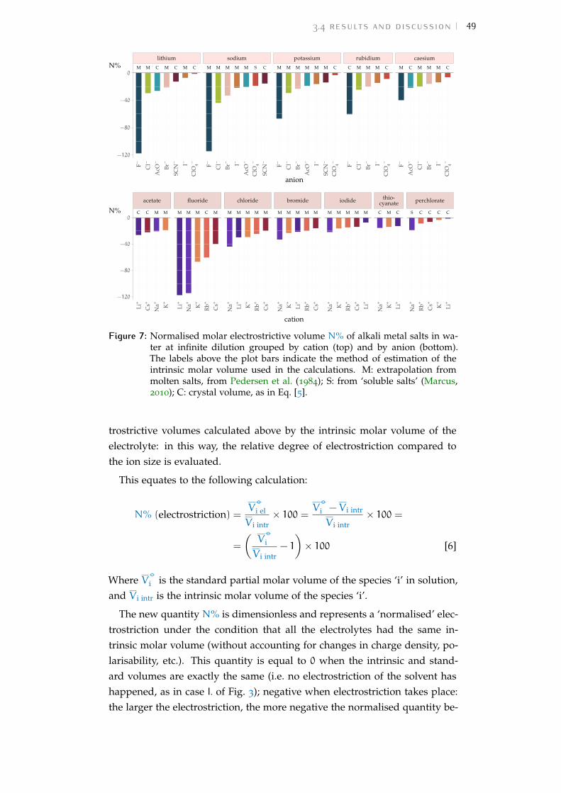
3.4 results and discussion 49
MM CM MC C MM SM M M C MM CM MM M MM CC M MM CM MC
lithium sodium potassium rubidium caesium
Br–
Cl–
ClO
–4F
– I–
AcO
–
SCN
–
Br–
Cl–
ClO
–4F
– I–
AcO
–
SCN
–
Br–
Cl–
ClO
–4F
– I–
AcO
–
SCN
–
Br–
Cl–
ClO
–4F
– I–
Br–
Cl–
ClO
–4F
– I–
AcO
–
−120
−80
−40
0
anion
N%
C MC M MMM M C MMMM M MM MM M MM MM M M CC C C CS C
acetate fluoride chloride bromide iodide thio-cyanate perchlorate
Cs+
K+
Li+
Na+
Cs+
K+
Li+
Na+
Rb+
Cs+
K+
Li+
Na+
Rb+
Cs+
K+
Li+
Na+
Rb+
Cs+
K+
Li+
Na+
Rb+
K+
Li+
Na+
Cs+
K+
Li+
Na+
Rb+
−120
−80
−40
0
cation
N%
Figure 7: Normalised molar electrostrictive volume N% of alkali metal salts in wa-ter at infinite dilution grouped by cation (top) and by anion (bottom).The labels above the plot bars indicate the method of estimation of theintrinsic molar volume used in the calculations. M: extrapolation frommolten salts, from Pedersen et al. (1984); S: from ‘soluble salts’ (Marcus,2010); C: crystal volume, as in Eq. [5].
trostrictive volumes calculated above by the intrinsic molar volume of theelectrolyte: in this way, the relative degree of electrostriction compared tothe ion size is evaluated.
This equates to the following calculation:
N% (electrostriction) =V−◦i el
V i intr× 100 = V
−◦i − V i intr
V i intr× 100 =
=
(V−◦i
V i intr− 1
)× 100 [6]
Where V−◦i is the standard partial molar volume of the species ‘i’ in solution,
and V i intr is the intrinsic molar volume of the species ‘i’.
The new quantity N% is dimensionless and represents a ‘normalised’ elec-trostriction under the condition that all the electrolytes had the same in-trinsic molar volume (without accounting for changes in charge density, po-larisability, etc.). This quantity is equal to 0 when the intrinsic and stand-ard volumes are exactly the same (i.e. no electrostriction of the solvent hashappened, as in case I. of Fig. 3); negative when electrostriction takes place:the larger the electrostriction, the more negative the normalised quantity be-

50 electrostriction
comes. Two sub-cases can be identified when N% is negative: −100% <
N% < 0 when the molar volume of the electrolyte is positive (case II.of Fig. 3), whereas N% < −100% for case III. of Fig. 3, when the molarvolume of the electrolyte is smaller than 0 and therefore the final solutionvolume is even smaller than the original pure solvent volume. Finally, N%is positive when expansion of the solvent happens as in case IV. of Fig. 3.
The resulting plots for electrolytes in water are in Fig. 7. The plots for allthe remaining solvents are in the Appendix A.4 (Figs. 55 to 65). Tables 18and 19 summarise the series observed in the different solvents, groupingelectrolytes by cation and anion, respectively.
The effect of the normalisation is an even more homogeneous picture forthe anion behaviour (Table 18 versus Table 16), where the Hofmeister seriesis nearly universal, with the only exception being lithium salts in ace.
Significantly for the cations shown in Table 19: the reverse lyotropic seriesis preponderant, as it was for the standard partial molar volumes (Table 14).The most variability in behaviour across solvents is observed for polyatomicions, for which the Hofmeister series and reverse Hofmeister series are ob-served and an altogether new series occurs as well. Polyatomic ions have per-manent multipole moments due to the asymmetrical distribution of charge,therefore it is unsurprising that electrostriction does not follow the sameseries evident for the monoatomic anions. If the polyatomic anions areset aside, the reverse lyotropic series is nearly universal. This is a dra-matic change from the pre-normalised electrostrictive volumes summarisedin Table 17. The preponderance of the reverse lyotropic series producedfrom the normalised electrostrictive volumes for cations across a wide rangeof solvents is in accordance with the domination of the reversed lyotropicseries for cations derived from the standard molar volumes, adding weightto the argument that the cations fundamentally give rise to a reversed lyo-tropic series independent of the solvent.

3.4 results and discussion 51
Table 18: Specific-ion effects series exhibited in the normalised electrostrictivevolume of electrolytes, N%: anions arranged by a common cation.
cation protic solvents aprotic solvents
water meoh etoh fa nmf eg pc ec dmso ace mecn dmf
Li+ F– F– F– F– Br– F– Cl– I– F– Cl– Cl– Cl–
Cl– Cl– Cl– Br– Cl– Cl– Br– ClO4– Cl– Br– Br– Br–
AcO– Br– Br– Cl– SCN– Br– I– Br– ClO4– I– I–
Br– I– I– SCN– I– I– ClO4– I– I– SCN– ClO4
–
SCN– SCN– AcO– I– ClO4– ClO4
– ClO4–
I– ClO4– ClO4
–
ClO4–
Na+ F– F– F– F– Cl– F– Cl– I– F– Cl– Cl– Cl–
Cl– Cl– Cl– Cl– Br– Cl– Br– ClO4– Cl– ClO4
– Br– Br–
Br– Br– Br– Br– I– Br– I– Br– Br– I– I–
I- I– I– I– ClO4– I– ClO4
– I– I– SCN– ClO4–
AcO– SCN– AcO– ClO4– SCN– ClO4
– ClO4–
ClO4– ClO4
– SCN–
SCN–
K+ F– F– F– Cl– Br– F– Cl– I– F– Cl– Cl–
Cl– Cl– Cl– F– Cl– Cl– I– ClO4– Cl– Br– Br–
Br– Br– Br– Br– I– Br– Br– Br– I– I–
AcO– I– I– I– SCN– I– ClO4– I– SCN– ClO4
–
I– SCN– AcO– SCN– ClO4– ClO4
– ClO4–
SCN– ClO4– ClO4
–
ClO4–
Rb+ F– F– F– F– I– Cl– F– Cl– Cl–
Cl– Cl– Cl– Cl– F– I– Cl– Br– Br–
Br– Br– Br– Br– Cl– Br– Br– I– I–
I– I– I– I– Br– ClO4– I– ClO4
– ClO4–
ClO4– ClO4
– ClO4– ClO4
–
Cs+ F– F– F– Cl– Br– F– Cl– F– Cl– Cl–
AcO– Cl– Cl– Br– Cl– Cl– I– Cl– Br– Br–
Cl– Br– Br– F– I– I– Br– Br– I– I–
Br– I– I– I– ClO4– Br– ClO4
– I– ClO4– ClO4
–
I– ClO4– AcO– ClO4
– ClO4–
ClO4–
For each cation, the anions are listed from largest (top) to smallest (bottom) normalised electrostrictivevolume. The cell background is coloured as indicated in the legend above if that order of ions correspondsto a known sie series.
Hofmeister lyotropic
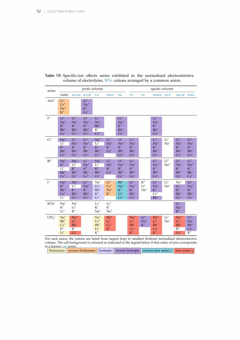
52 electrostriction
Table 19: Specific-ion effects series exhibited in the normalised electrostrictivevolume of electrolytes, N%: cations arranged by a common anion.
anion protic solvents aprotic solvents
water meoh etoh fa nmf eg pc ec dmso ace mecn dmf
AcO– Li+ Li+
Cs+ Na+
Na+ K+
K+ Cs+
F– Li+ Li+ Li+ Li+ Li+ Li+
Na+ Na+ Na+ Na+ Na+ Na+
K+ K+ K+ Rb+ K+ K+
Rb+ Rb+ Rb+ K+ Rb+ Rb+
Cs+ Cs+ Cs+ Cs+ Cs+ Cs+
Cl– Na+ Li+ Li+ Na+ Li+ Li+ Li+ Li+ Li+ Li+ Li+
Li+ Na+ Na+ Li+ Na+ Na+ Na+ Na+ Na+ Na+ Na+
K+ K+ K+ K+ K+ K+ K+ K+ K+ K+
Rb+ Rb+ Rb+ Rb+ Cs+ Rb+ Rb+ Rb+ Rb+ Rb+
Cs+ Cs+ Cs+ Cs+ Cs+ Cs+ Cs+ Cs+ Cs+
Br– Na+ Na+ Li+ Na+ Li+ Li+ Li+ Li+ Li+ Li+ Li+
K+ Li+ Na+ Li+ Na+ Na+ Na+ Na+ Na+ Na+ Na+
Li+ K+ K+ K+ K+ K+ K+ K+ K+ K+
Rb+ Rb+ Rb+ Rb+ Cs+ Rb+ Rb+ Rb+ Rb+ Rb+
Cs+ Cs+ Cs+ Cs+ Cs+ Cs+ Cs+ Cs+ Cs+
I– Na+ Na+ Li+ Na+ Li+ Rb+ Li+ K+ Li+ Li+ Na+ Li+
K+ Li+ Na+ Cs+ Cs+ Na+ Na+ Li+ Na+ Na+ Li+ Na+
Rb+ K+ K+ Rb+ Na+ K+ K+ Na+ K+ K+ K+
Cs+ Rb+ Rb+ K+ K+ Li+ Rb+ Cs+ Rb+ Rb+
Li+ Cs+ Cs+ Li+ Cs+ Cs+ Rb+ Cs+ Cs+
SCN– Na+ Na+ Li+ Li+ Li+
K+ Li+ K+ K+ Na+
Li+ K+ Na+ Na+ K+
ClO4– Na+ Na+ Na+ Na+ Na+ Li+ Na+ Li+ Na+ Li+
Rb+ Li+ Cs+ Li+ Li+ Na+ Li+ Na+ Li+ Na+
Cs+ Rb+ Rb+ Cs+ Rb+ K+ Rb+ Rb+ Rb+
K+ K+ Li+ K+ Cs+ Cs+ K+ Cs+
Li+ Cs+ K+ K+ K+ Cs+ K+
For each anion, the cations are listed from largest (top) to smallest (bottom) normalised electrostrictivevolume. The cell background is coloured as indicated in the legend below if that order of ions correspondsto a known sie series.
Hofmeister reverse Hofmeister lyotropic reverse lyotropic reverse new series 1 new series 3
3.4 results and discussion 53
3.4.4 General implications
From this work a number of conclusions regarding sie can be drawn.
It is apparent that the ordering of sie for the standard molar volumes andthe normalised electrostriction of electrolytes at infinite dilution is independ-ent of the solvent. This ordering follows a Hofmeister series for anions anda reversed lyotropic series for cations, which corresponds to smaller ‘harder’cations and anions having a smaller intrinsic volume V
−◦i and causing a lar-
ger normalised electrostriction N% than large, ‘soft’ cations and anions. Asa consequence, the grouping usually associated with the Hofmeister series isrespected for anions. That is the ‘structure makers’ or ‘kosmotropes’ whichare ions small in size and with high surface charge density and small polar-isability give rise to the largest electrostriction. This does not hold for thecations, where the Hofmeister series ordering is lost and an ordering thatfollows the reverse lyotropic series which is determined by the cation size isinstead in place.
This solvent-independence of electrostriction in the limit of infinite dilu-tion demonstrates that, at a fundamental level, such as for bulk propertiesof very diluted solutions, the ordering of sie are solely a property of theions and the only essential ingredient for sie to happen is the presence ofelectrolytes. As most experimental observations of sie are made at moder-ately high to high electrolyte concentrations, this may lead to the erroneousconclusion that these effects are only manifest at high concentrations. In factneither surfaces nor higher concentrations are needed. Of course the sol-vents do matter in that they mediate the strength of the effects. This findingis corroborated by the trends found in Chapter 2 for bulk properties such asthe limiting molar conductivity (lmc) and the viscosity B-coefficient (vbc),where a lyotropic series is predominant for the alkali metals cations anda Hofmeister series for the anions. Whereas other experiments involvingions at high concentration and surfaces result in a perturbation to the fun-damental series observed here, as illustrated in Table 13 of Chapter 2. Theseperturbations likely arise due to a complex interaction of ion pairing, disper-sion forces, and solvation both in the bulk and at interfaces. Furthermore,the balance of these effects will depend on temperature as well as the specif-ics of the solvent and surfaces (Leontidis, 2017). An improved understandingof the suite of sie observed may therefore be gained by considering themas perturbations to the fundamental series observed here in the simplestsystems.
The homogeneity in behaviour of electrostrictive phenomena must notshadow the fact that ion solvation mechanisms differ greatly across solvents.Electrostriction is only one consequence of ion solvation and does not cap-ture the local ion-solvent interactions or the structure of the solvent around
54 electrostriction
solvated ions. The chemical properties, molecular size and polarisability ofthe solvents vary widely. The interactions between ions and solvent are re-flected in selective ion- solvent interactions. These have been shown to varygreatly for solvents of different polarisability, leading to different trends insolvation (Arslanargin et al., 2016; Pollard and T. L. Beck, 2017). The ther-modynamics of solvation across solvents and the effect of ions on solventstructure and on solvent dynamics needs to be considered to obtain a com-prehensive physical picture. Some of these matters are addressed in thefollowing chapters.
How might this information be useful in furthering our understandingof sie? This analysis tells us that calculations and simulations of sie indilute solutions should be able to reproduce the Hofmeister series for anionsand the lyotropic series for cations without specifically accounting for thesolvent, supporting an approach already being employed (Duignan, Baerand Mundy, 2016). The details of the solvent will matter in determiningthe magnitude of the effect. The interpretation I propose for this evidence isthat, when the system becomes more complex, for instance because a surfacecomes into play, or because the electrolyte concentration is increased, thosefundamental sie are perturbed and both surfaces and the solvent come intoplay and determine their final ordering.
3.5 conclusionsIn this chapter, the trends of sie for standard molar volumes and standardelectrostrictive volumes have been analysed. In order to compare acrossions and solvents, a normalisation of the electrostrictive volumes has beenperformed. This work evidences the presence of sie at low concentration, anotion that has often been disregarded in the literature, where many authorsassociate sie only with higher salt concentrations (Parsons and Salis, 2016).This is perhaps due to the magnitude of these effects being small for manymeasurements at low concentration, and in some systems sie may only berevealed once electrostatic effects have been quenched by screening.
Electrostriction is an ion-specific effect in all of the electrolyte solutionsconsidered. This confirms that, with respect to sie, water is not a ‘special’solvent. This also rejects the idea of an exclusive association between theexistence of sie and the presence of a hydrogen-bonding network: aproticsolvents show ion specificity as well, indeed ions in all solvents show ionspecificity. Further, the complexity conferred by ion specificity is necessaryfor life, but ion specificity is not restricted to aqueous solutions.
These findings support the hypothesis that the ordering of sie is funda-mentally due to properties of the ions themselves and that this fundamental

3.5 conclusions 55
ordering is exhibited experimentally under appropriate circumstances. Thisis exemplified by the partial molar volume and normalised electrostrictionof anions following a Hofmeister series whilst the cations follow a reverselyotropic series. The quantitative connection between these series and theindividual properties of the ions is not trivial and remains the realm of act-ive efforts in this field. This outcome is important for the understanding ofsie. In models of bulk properties of solvents in the limit of infinite dilution,the specific nature or the granularity of the solvent should not determine theorder of the sie.


4 V O LC A N O P LOT S
This chapter is reproduced with minor changes from:
V. Mazzini and V. S. J. Craig (2018), ‘Volcano Plots Emerge from a Sea ofNon-aqueous Solvents: The Law of Matching Water Affinities Applies acrossAll Solvents.’ Submitted.
4.1 introductionUnderstanding of sie, and especially phenomena such as the reversal of theHofmeister series, has benefited greatly from the empirical ‘law of match-ing water affinities (lmwa)’, enunciated by Collins (1997). This law predictsthat, in aqueous solutions, ion pairs are formed by cations and anions withmatching size (charge density). Collins explains that ‘the small ions of op-posite charge form contact ion pairs because of electrostatic attraction; thelarge ions of opposite charge form contact ion pairs because this releasesweakly hydrated water, which becomes strongly interacting water in bulksolution’ (Collins, 2012). This is an extension of the ‘like seeks like’ rule. Col-lins used ‘volcano plots’ as one of the theoretical foundations for the lmwa.The term ‘volcano plot’ arises from the shape of the plot which resembles acinder cone in profile. Such plots were first published by Morris in responseto a suggestion from Fajans, who first enunciated a ‘competition principle’regarding the dissolution of crystalline electrolytes and their interaction insolution.
In this chapter the relationship between volcano plots and the lmwa is ex-amined, and the volcano plots are extended to non-aqueous solvents, firstlyto test the existence of such volcano relationships in non-aqueous solvents,and secondly to test the hypothesis that trends in ion specificity only dependon the ions and not on the solvent.
Although sie are often interpreted as arising from the interaction of ionswith water, the evidence presented in the previous chapter shows that uni-versal ion-specific trends are observed across a wide range of solvents, im-plying that trends in ion-specificity arises from the ions independently of thesolvent (although, the solvent mediates the magnitude of the effect).
57
58 volcano plots
4.2 energies related to the solvation processAs the present chapter deals with the thermodynamics of solvation, I intro-duce here the definitions of the quantities that are going to be discussed: theenergies and the entropy related to the solvation of ions and the dissolutionof electrolytes.
The enthalpy of solvation ∆abs. soln.H is the heat exchanged when a sub-stance is transferred from a vacuum (or the gas phase) to the solvent atconstant pressure (McNaught and Wilkinson, 1997). This quantity includescontributions from the formation of a cavity in the solvent, the reorientationof the solvent molecules and the formation of both electrostatic and disper-sion interactions between the solute and the solvent. The Gibbs free en-ergy of solvation is calculated using its fundamental thermodynamic defin-ition: ∆abs. soln.G = ∆abs. soln.H− T∆abs. soln.S, where ∆abs. soln.S is the entropyof solvation of the species and ∆abs. soln.H is the enthalpy of solvation. Ineach case the relevant change is the change between the species in solutionand the species in the ideal gas phase; T is the absolute temperature in K.T = 298.15K for all the quantities discussed here.
The standard enthalpy ∆fH−◦ , entropy ∆fS
−◦ , and Gibbs free energy ∆fG−◦
of formation refer instead to the formation of the species of interest (in ourcase either aqueous electrolyte, gaseous ions or crystalline salt) from theconstituent elements in their respective standard states.
The absolute standard molar enthalpy of solvation of a salt ∆abs. soln.H−◦ is the
change in enthalpy when one mole of gaseous ions are dissolved in an infin-itely large quantity of solvent. It is calculated as the sum of the ∆abs. soln.H
−◦
of the constituent ions and is referred to as ‘absolute enthalpy of solvation’in the following sections for brevity.
The standard molar enthalpy of dissolution of the crystalline salt ∆soln.H−◦ is
calculated as the difference between the standard molar enthalpy of forma-tion of the infinitely dilute aqueous electrolyte ∆fH
−◦ (MX, aq) and the stand-ard molar enthalpy of formation of the pure electrolyte ∆fH
−◦ (MX, cr) (whichin this case refers to crystalline salts, as none of the alkali metal halides aregaseous or liquid in standard conditions). It will be referred to as ‘enthalpyof dissolution’ in the following sections.
Analogous definitions stand for the absolute standard molar Gibbs freeenergy of solvation of a salt ∆abs. soln.G
−◦ and the standard molar Gibbs freeenergy of dissolution of the crystalline salt ∆soln.G
−◦ .
These two quantities are represented on the axes of the ‘classic’ volcanoplots. Figure 8 illustrates the relationship between the different states andrelative solvation energies.
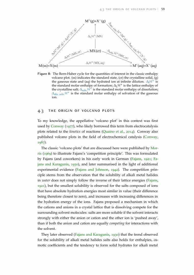
4.3 the origin of volcano plots 59
M(ss)+X(ss) M+(aq)+X– (aq)
MX(cr)
M+(g)+X– (g)
∆fH−◦ (MX, aq)
∆LH−◦ (MX)
∆ fH−◦ (M
+ , g) +∆ fH
−◦ (X– , g)
∆ fH−◦ (MX, cr)
∆abs. soln. H −◦
(M +, g) +∆
abs. soln. H −◦(X –, g)
∆soln.H−◦(MX, cr)
Figure 8: The Born-Haber cycle for the quantities of interest in the classic enthalpyvolcano plot. (ss) indicates the standard state, (cr) the crystalline solid, (g)the gaseous state and (aq) the hydrated ion at infinite dilution. ∆fH
−◦ isthe standard molar enthalpy of formation; ∆LH
−◦ is the lattice enthalpy ofthe crystalline salt; ∆soln.H
−◦ is the standard molar enthalpy of dissolution;∆abs. soln.H
−◦ is the standard molar enthalpy of solvation of the gaseousion.
4.3 the origin of volcano plotsTo my knowledge, the appellative ‘volcano plot’ in this context was firstused by Conway (1977), who likely borrowed this term from electrocatalysisplots related to the kinetics of reactions (Quaino et al., 2014). Conway alsopublished volcano plots in the field of electrochemical catalysis (Conway,1987).
The classic ‘volcano plots’ that are discussed here were published by Mor-ris (1969) to illustrate Fajans’s ‘competition principle’. This was formulatedby Fajans (and coworkers) in his early work in German (Fajans, 1921; Fa-jans and Karagunis, 1930), and later summarised in the light of additionalexperimental evidence (Fajans and Johnson, 1942). The competition prin-ciple stems from the observation that the solubility of alkali metal halidesin water does not simply follow the inverse of their lattice energies (Fajans,1921), but the smallest solubility is observed for the salts composed of ionsthat have absolute hydration energies most similar in value (their differencebeing therefore closest to zero), and increases with increasing differences inthe hydration energy of the ions. Fajans proposed a mechanism in whichthe cations and anions in a crystal lattice that is dissolving compete for thesurrounding solvent molecules: salts are more soluble if the solvent interactsstrongly with either the anion or cation and the other ion is ‘pushed away’,than if both the anion and cation are equally competing for interactions withthe solvent.
They later observed (Fajans and Karagunis, 1930) that the trend observedfor the solubility of alkali metal halides salts also holds for enthalpies, os-motic coefficients and the tendency to form solid hydrates for alkali metal
60 volcano plots
halides. Their measurements of the refractive index of electrolyte solutionsshowed that the same competition principle can be extended to electrolytesin solution, and they infer the formation of association ion pairs for ions ofsimilar absolute free energy of hydration (Fajans and Johnson, 1942). Thefact that anions and cations of the same size do not have the same absolutehydration enthalpy (anions have a larger hydration enthalpy than cations ofthe same size), demonstrates, according to Fajans and Johnson, that whatgenerates the volcano trends is the difference in hydration enthalpy ratherthan the difference in ionic radii of the ions constituent the salt. Therefore,according to the authors, the two quantities cannot be used interchangeablyand it is the hydration energy that causes the volcano trend. They attribute thedifference in hydration enthalpy of the anions and cations to an asymmetryin the properties of the water molecule. However, when analysing trends inthe osmotic coefficients with concentration, they observe that the differencein the hydration enthalpies is not valid over the whole concentration rangeand also that a simple property cannot explain the behaviour of electrolytes.
Later, when Morris published the volcano plots, he supported the explan-ation proposed by Fajans and made no additional remarks regarding theorigin of the volcano trend (Morris, 1969).
4.3.1 Early literature citing volcano plots
Before the ‘revival’ of volcano plots initiated by Collins (1997), who includedthem as evidence of the ‘law of matching water affinities (lmwa)’ (discussedlater in Section 4.4), the significance of the ‘striking’ volcano relationshiphad been discussed explicitly by Conway (1977). He showed that, on a semi-quantitative level, the enthalpy of dissolution of a salt crystal in water canbe expressed as a function of the reciprocal sums of the anionic and cationicradii, r− and r+:
∆hydr.H(salt) =−A
r+ + r−−
(ze)2
2
(1−
1
εR
)(1
r++1
r−
)= [7]
=−A
r+ + r−−
(ze)2
2
(1−
1
εR
)(r+ + r−)
1
r+r−[8]
Where A is the is the Madelung constant for the crystal lattice and ze is theformal charge (z = 1 for the alkali metal halides). Equation [8] has a max-imum for cationic and anionic radii that are closest in value, that is, whentheir difference is closest to zero. Conway therefore dismisses the ‘mechan-istic’ interpretation given by Fajans and Johnson (1942) and supported byMorris (1969), labelling the argument of the preferential competition of theion for the solvent as unnecessary, as the volcano shape arises naturally as the
4.4 the law of matching water affinities 61
result of the mathematical form of the dissolution enthalpy (or Gibbs free energy)function (Conway, 1977).
Later, Jenkins and Pritchett (1984) use a fitting of the volcano plot todetermine absolute single ion values of several thermodynamic properties.They also assume a volcano-like relationship between the dissolution enthal-pies/Gibbs free energies (y-axis) and the difference of the ionic viscosityB-coefficient Bη (x-axis).
The volcano plots of Morris (1969) have been invoked on a number ofoccasions to explain the solubility of compounds in water (Crawford andKlapötke, 1999; Vishnu and Mishra, 1981; J.-H. Yang et al., 2007).
4.4 the law of matching water affinitiesThe volcano plots of Morris (1969) were cited by Collins (1997) as a ther-modynamic foundation of his empirical ‘law of matching water affinities(lmwa)’. The lmwa states that, in solution, oppositely charged ions (aswell as charged groups) that have similar affinity for water spontaneouslylose part of their hydration shells to associate and form a contact ion-pair(two ions interacting directly with no water molecules in-between).
Collins built his argument on the volcano plots, on thermodynamic obser-vations such as the entropy of water molecules near an ion, and on experi-mental evidence (viscosity B-coefficient, nmr, gel sieving chromatography,neutron and x-ray diffraction, etc.). Collins states that oppositely chargedions in solution tend to form contact (or ‘inner-sphere’) ion pairs when theyhave ‘matching water affinity’. Here water affinity refers to the strength of in-teraction of the ion or charged moiety with water, and can be expressed viaa range of properties of ions in solution. For volcano plots, Collins uses theabsolute Gibbs free energy of hydration of the gaseous ion as a measure ofits affinity for water. The water affinity is directly related to the charge dens-ity on the ion (which is proportional to size for spherical monoatomic ions).The smaller the ion, the greater the charge density. Collins argued that ionstend to associate when their interactions are stronger than their interactionwith water (they are both small) or when their interaction with water is lessfavourable than the water-water interaction (when both ions are large). Ionswith comparable (‘matched’) hydration enthalpies or free energies form saltsthat are the least soluble. It is argued that this is because ions with matchedcharge densities have comparable interactions with water and tend to forminner-sphere ion pairs in solution. Therefore, according to Collins, chargedand also noncharged moieties in solution will prefer to associate with moi-eties of matching absolute free energies of hydration. This is an extension ofthe ‘like dissolves like’ principle. This framework has proved successful for

62 volcano plots
rationalising a variety of observations, such as ion pumps, the interactionsof ions with proteins, and ion selectivity in ion exchange chromatography.
The lmwa was re-stated and expanded in four subsequent papers (Col-lins, 2004, 2006, 2012; Collins, Neilson et al., 2007). After the publicationof the lmwa, the terms and concepts ‘volcano plots’ and lmwa are citedindistinguishably. A similar ‘like seeks like’ principle has been formulatedby Lyklema (2003) when reviewing sie on the stability of colloids: smallcations are more effective at destabilising colloids that have small negativelycharged surface sites (i.e. Li+ is more effective than Rb+ in precipitating TiO2,with surface sites of deprotonated hydroxyl groups) and vice versa (AgI col-loids are precipitated at lower concentrations of RbI than LiI). An older andanalogous concept is the hard-soft principle of acids and bases (hsab) (Pear-son, 1963). This states that ‘hard’ (nonpolarisable) acids prefer to bind to‘hard’ bases, and ‘soft’ (polarisable) acids prefer to bind to ‘soft’ bases. Thisinfluences a large number of phenomena in solution, such as the rates ofnucleophilic substitution reactions and the formation and stabilisation ofmetal-ligand complexes (Pearson, 1963).
4.5 brief review of recent volcano plot studiesThe lmwa concept has been embraced by the scientific community. Thepapers introducing the lmwa concept (Collins, 1997, 2004, 2006, 2012; Col-lins, Neilson et al., 2007) have had a large impact, in fields spanning from(bio)chemistry and (bio)physics to pharmacology, physiology, food science,materials science, polymer science and microbiology. There is no doubt thatthe lmwa has been a very helpful framework across disciplines, advancingthe understanding of sie both experimentally and theoretically, as recog-nised by many authors (Kunz and Neueder, 2009; Pollard and T. L. Beck,2016; Schmidtchen, 2010).
An important further step is the extension of the lmwa to charged surfact-ant headgroups relevant in biology and colloid science (carboxylate, phos-phate, sulfate, sulfonate) by Vlachy, Jagoda-Cwiklik et al. (2009). A Hofmeis-ter ordering of these headgroups based on computational and experimentaldata was proposed, and the lmwa was used to rationalise the interactionof such groups with aqueous ions. Using this generalised approach, thebehaviour of polyelectrolytes, surfactants and lipids were predicted withsuccess. Subsequent experiments from the same group supported this ap-proach (Vlachy, Drechsler et al., 2009).
The general predictions of the lmwa have been confirmed by various ex-periments. In water, x-ray absorption spectroscopy indicates that sodiumbinds more strongly than potassium to the acetate anion (Uejio et al., 2008).

4.5 brief review of recent volcano plot studies 63
Also, investigations with nir (near infra-red) spectroscopy find that the de-pletion of water from hydration shells of alkali metal ions varies among ionsin accordance with the lmwa (Kojic et al., 2014). Moreover, picoseconddynamics of water at a proteins’ surface (and hence the protein stability)is altered by anions following the opposite trend to the dynamics of bulkwater, which is in agreement with the lmwa (Aoki et al., 2016). However,2DIR spectroscopy (Sun et al., 2013) reveals the existence of contact ion pairsin solution between SCN– and Ca2+ or Mg2+. This is in opposition to thelmwa.
The lmwa has been employed to rationalise a number of behaviours inelectrolyte solution. These include the retention of proteins on cation-ex-change absorbents (DePhillips and Lenhoff, 2001), the interaction of poly-electrolytes with halide ions (Lukšic, Boncina et al., 2012), the rheologicalbehaviour of copolymers (Obiweluozor et al., 2014) and the salt-dependenceof the interaction potential between a colloidal polystyrene particle and a flatglass surface (Ao et al., 2011). The reactivity in aqueous solution (Trompette,2015) and ionic liquids (Lin et al., 2016) also belongs to the list. In addition,the lmwa framework supports the observed solubility of anionic surfact-ants (Klein et al., 2009), the influence of counterions and coions on the cmcof mixed anionic-cationic surfactant systems (Hao, Deng et al., 2012; Hao, N.Yang et al., 2016; Nan, He et al., 2013; Nan, Xu et al., 2015), the phase beha-viour of cationic lipids (Tarafdar et al., 2013), and the phase behaviour, sta-bility and morphology of naturally occurring marine surfactants (T. Zhanget al., 2016). The aggregation behaviour of dyes in aqueous solution (Mooiand Heyne, 2012; Mooi, Keller et al., 2014) and their interaction with surfact-ants (Srivastava and Ismail, 2014) can be qualitatively accommodated by thelmwa as well.
Regarding peptides and proteins, contrasting experimental evidence hasbeen reported. Anion interactions with charged sites of proteins (Fox et al.,2015), and also the interaction of divalent and trivalent cations with a negat-ively charged protein in the native membrane environment (Batoulis et al.,2016), confirm the lmwa. On the other hand, the empirical rule falls short ofexplaining the effects of monovalent cations on enzymatic activity (Medda,Salis et al., 2012), or the concentration dependence of the cation effectivenessin promoting hemoglobin aggregation (Medda, Carucci et al., 2013). In addi-tion, while the association strength of monovalent cations with carboxylatemoieties of a polypeptide follows the lmwa (with the exception of NH4
+
and Li+), the divalent ions do not follow it at all (Kherb et al., 2012).
Theorists have been looking to provide foundations for the lmwa (Astha-giri et al., 2000; Gao, 2011; Merchant and Asthagiri, 2009; Shi and T. Beck,2017). They all agree that continuum models and classical models are in-sufficient to quantitatively describe electrolyte solutions, although they can
64 volcano plots
partially capture their behaviour. For instance, the weak pairing of differ-ently sized ions is attributed to a ‘shadowing’ effect of the larger ion, whichprevents the smaller ion from favourably interacting with the solvent (Lundet al., 2010). Other groups (Duignan, Parsons et al., 2014c; Parsons, Boström,Lo Nostro et al., 2011) propose the inclusion of dispersion interactions toreach a quantitatively descriptive and physically meaningful picture, thataccounts for the lmwa.
A number of md are in agreement with the predictions of the lmwa (Fen-nell et al., 2009; C.-W. Liu et al., 2014; Soniat et al., 2016; Xie et al., 2016).The predictions of the lmwa have also been used as benchmarking for mdsimulations (Lukšic, Fennell et al., 2014), and to make reasonable guessesof values for which experimental data are absent (Moreira and Firoozabadi,2010). Some results are in disagreement with the lmwa, as in the case ofmd simulations that only find solvent-shared ion pairs and no contact ionpairs (Hess and van der Vegt, 2009), and the substantial deviation foundwhen ions are of a similar size to the water molecule (Q. Zhang et al., 2014).
4.5.1 Other reports of volcano trends
Other authors have reported volcano or volcano-like trends. They are listedbelow and summarised in Table 20.
Dzubiella et al. (2009) in Kunz’s book about sie (Kunz, 2009), follow thesame reasoning as Conway (1977), and argue that the ion-dependence ofmany collective properties of electrolytes that are obtained as the differenceof an ion-pair property and a single-ion property will show a peak or valleywith respect to the difference of the radii of the single ions. For instance,the enthalpy of dissolution of an electrolyte is obtained as the differencebetween the sum of the absolute enthalpies of hydration of the gaseous ions(properties of the single ions) and the lattice enthalpy (a property of the ionpair) and the enthalpy of dissolution does indeed show a maximum whenplotted against the difference of the radii of the constituent ions. The po-sition of the peak will change for different properties. In their simplifiedmodel, they increase the radius of the cation by a quantity of the order ofthe lengthscale of the O – H bond in the water molecule (0.08nm), to accountfor the fact that the cations are solvated by the oxygen of water, which hasa non-vanishing radius. The plot of the enthalpy of dissolution of electro-lytes against the difference of the radii of the constituent ions (anion minuscation) has a maximum in correspondence to such difference amounting to0.08nm (Dzubiella et al., 2009). Despite the model being basic and thereforenot being capable of quantitative agreement with experimental values, theauthors reach the same conclusions as Conway (1977): due to its functionalform, the enthalpy of hydration of an electrolyte is bound to have a max-

4.5briefreviewofrecentvolcanoplotstudies65
Table 20: Volcano plots reported in the literature. The symbols are defined in the text.
reference x-axis y-axis additional information
Morris, 1969 ∆abs. hydr.H−◦ (X–, g) −∆abs. hydr.H
−◦ (M+, g) ∆hydr.H−◦ (MX, cr) to illustrate Fajans’s competition principle
∆abs. hydr.G−◦ (X–, g) −∆abs. hydr.G
−◦ (M+, g) ∆hydr.G−◦ (MX, cr)
Dzubiella et al., 2009 rM+ − rX– ∆hydr.H−◦ (MX, cr) fitted by parabolas
Kherb et al., 2012 ∆abs. hydr.H−◦ (CH3COO−) −∆abs. hydr.H
−◦ (Mz+) Kd(RCOO−Mz+) inverted volcano for monovalent cations, ex-cept NH4 and Li+; no volcano trend fordivalent cations
Gujt et al., 2014 ∆abs. hydr.G−◦ (M+) −∆abs. hydr.G
−◦ (X−) S
Ka
Batoulis et al., 2016 z/refficacy in clustering amembrane protein
no volcano trend obtained when z, crystalradius, volume, polarizability or softness areplotted on the x-axis
Bη
∆abs. hydr.G−◦ /CN
Soniat et al., 2016 ∆abs. hydr.G−◦ (X−) −∆abs. hydr.G
−◦ (M+) φ inverted volcano
Arslanargin et al., 2016 ∆abs. hydr.H−◦ (X−) −∆abs. hydr.H
−◦ (K+) ∆hydr.H−◦ (KX, cr) opposite trend than KX in water

66 volcano plots
imum when the difference in radii between anion and cation has a certainvalue. This value corresponds to zero in Conway’s model, and to 0.08nm inthe analysis of Dzubiella et al., as they account for the different sizes of thesolvating groups of the water molecule.
Kherb et al. (2012) show an inverted volcano for the association strengthof monovalent cations with the carboxylate moieties of a polypeptide (al-though NH4
+ and Li+ are exceptions), but the divalent ions do not follow avolcano trend. Gujt et al. (2014) find a volcano relationship between the asso-ciation constants of eight alkali halides calculated from their conductivity atlow concentration and the difference of the Gibbs free energies of hydrationof the cation and anion. Soniat et al. (2016) show the volcano relationshipbetween the osmotic coefficients φ of the alkali halides and the differencein hydration free energies of the constituent ions (this had been noted earlyon by Fajans as well). Batoulis et al. (2016) study the oligomerisation bydifferent cations (mostly divalent and trivalent) of a protein in a native mem-brane environment. They find that plots of the protein clustering efficacy ofcations versus the ion charge-to-radius ratio, or hydration energy, or waterviscosity B-coefficient show a volcano trend in which Sr2+ marks the max-imum. They conclude that the most effective ions at clustering are the onesthat have hydration energy closer to the acetate groups hydration energy inthe protein. Arslanargin et al. (2016), study the solvation of potassium hal-ides in ec and pc, by means of statistical mechanics and simulations. Theyplot the enthalpy of dissolution of the crystal against the difference of theionic hydration enthalpies they have computed, and the trend they obtainis ion-specific and in line with a volcano trend (see Section 4.5.3 for furtherdiscussion on those trends).
4.5.2 Limitations of the lmwa
The intuition built into the lmwa is formidable, but it is a simplistic modelwith intrinsic limitations (Kunz, 2010; Parsons, Boström, Lo Nostro et al.,2011; Shi and T. Beck, 2017). As such, it is important that the shortcomingsand inconsistencies are acknowledged if a predictive understanding of thebehaviour of ions and charged sites in solution is to be achieved.
A number of authors have pointed out weaknesses in the foundations ofthe lmwa. The first criticism is the usage of volcano plots to explain ion-ion interactions in solution. The quantities plotted on the volcano plots arestandard thermodynamic quantities. As such they refer to ions at infinitedilution and hence the application to ion-ion interactions is tenuous. Theconnection between the two physical situations of infinite dilution and finiteconcentrations has not been justified. An additional incongruence is the ex-planation for the interaction among large ions in solution. The justification
4.5 brief review of recent volcano plot studies 67
for the lmwa assumes that the interactions among large ions and water areless favourable than water-water interactions, however the hydration energyof large ions is large and favourable (negative), therefore this argument can-not be sustained. Large ions must be preferentially interacting for anotherreason, most likely due to attractive dispersion forces.
These observations were first brought forward by Lo Nostro and Ninham(2012), and reiterated and expanded by Duignan, Parsons et al. (2014c), whoproposed a different volcano plot based on the B coefficients from Bromley’stheory (Bromley, 1973) (not to be confused with the Jones-Dole viscosityB-coefficient Bη. They obtained a ‘reversed volcano’ with a clearer phys-ical meaning than the explanations behind the lmwa. Salis and Ninham(2014) attempted a reconciliation of the quantitative and qualitative views,as the theoretical basis for the lmwa is questionable but its predictions arecorrect, however, as yet, the quantitative theoretical approach proposed byNinham and collaborators has not been as broadly received. They argue thata theory that correctly treats electrostatics and quantum mechanical disper-sion forces can quantitatively predict the behaviour and association of bothcharged and non-charged ions and sites in solution. This theory develops awider framework which includes interactions between ions and unchargedsurfaces, in which the lmwa is contained as a sub-case. They propose thatsmall ions prefer to lose water molecules and interact directly as the smallsize gives rise to large interaction energies (in agreement with the lmwa);whereas large ions interact strongly by dispersion forces (in contrast to thelmwa which has these ions interacting weakly). When ions of different sizesinteract, neither dispersion forces nor electrostatic interactions are highly fa-vourable. The latter argument also explains the adsorption of large ions ontouncharged surfaces and uncharged protein moieties by means of dispersioninteractions.
4.5.3 The lmwa and nonaqueous solvents
The lmwa was proposed for water, and only three cases in the literaturewhere its concepts are discussed for non-aqueous solvents could be identi-fied.
Long et al. (2013) suggest the extension of the lmwa to a non-aqueoussolvent (meoh), which requires a name change to the lmsa (law of match-ing solvent affinities). They use lmsa to rationalise the ion-specific growthof a polyelectrolyte in water-meoh mixtures. However, in this work thesalt concentration is low, the system behaviour is complex and water-meohinteractions have not been considered.
Lin et al. (2016) have investigated aqueous tetraalkylammonium ionic li-quids as both solvents and catalysts for non-enzymatic regioselective acyla-

68 volcano plots
tions of glucose. In the reaction mechanism they propose, they also makeuse of the lmwa to explain the better performance of tetrabutylammoniumacetate with respect to tetramethylammonium acetate.
With regards to aprotic solvents, Arslanargin et al. (2016) show that thetrend of the dissolution enthalpy of crystals versus the computed hydrationenthalpies of potassium halides in pc and ec is ion-specific, and the trendin these solvents has a maximum for KF, whereas in water KI shows themaximum dissolution enthalpy.
4.6 results and discussionNoting that volcano plots have been used to explain the lmwa, which im-plies water as the solvent, I wish to verify their existence in non-aqueoussolvents. If verified, I wish to determine whether the trends in non-aqueoussolvents are the same as in water. A number of electrolyte solution proper-ties (y-axis) are therefore plotted against the difference of a property of theconstituent ions (x-axis) in this section, starting from the ‘classic’ volcanoplots.
Alternative interpretations of volcano plots exist. One approach placesinteractions of the ions with the solvent at the centre, attributing the vol-cano plot trends to the ion-solvent interaction, represented by the solvationenergy (Collins, 1997, 2004, 2006, 2012; Collins, Neilson et al., 2007; Mor-ris, 1969; Schmidtchen, 2010). Alternatively, volcano plots are attributed tothe characteristics of the ions: size, and the associated polarisability, surfacecharge density, etc. (Conway, 1977; Dzubiella et al., 2009). In the first case,solvent dependent trends that alter the volcano plots substantially betweensolvents are to be expected. In addition, the volcano plots should be ob-served also for electrolytes containing polyatomic anions with geometriesthat are neither spherical nor tetrahedral, such as thiocyanate and acetate.
4.6.1 Definition of a volcano plot
It is important to clarify the definition of a volcano plot that is going to beapplied in the ensuing sections. The term volcano plot refers to a scatter plotwhere the data trend follows an overturned ‘V’: it monotonically increasesin a linear (the adjective is loosely applied) fashion up to a maximum, andthen decreases, monotonically and linearly, with a slope of similar absolutevalue to the ascending section. A volcano trend is recognised here whentwo conditions are met. Firstly, a scatter plot of a particular property of anelectrolyte shows a maximum with respect to the difference in a particularproperty of the anions and cations making up the electrolyte. This may for

4.6 results and discussion 69
example be the difference in size. Secondly, the peak of the volcano (i.e. themaximum) occurs in a quite narrow interval of values of the difference in aparticular property of the ions. The plot is therefore quite symmetrical withrespect to a vertical axis that goes through the maximum, thus resemblingthe shape of a volcanic cinder cone in profile. When evaluating volcano plotsformed from electrolytes, the trend can be observed with a common cationfor a number of anions (anion trend) or with a common anion for a numberof cations (cation trend).
4.6.2 Methods and data sources
The dissolution energies of electrolytes in non-aqueous solvents were ob-tained via two stages. Firstly, the energies of dissolution of the crystallineelectrolytes in water were obtained as the difference of the hydration ener-gies of the ions composing the electrolyte minus the formation energy of thecrystalline electrolyte. The relationship of these thermodynamic quantitiesis illustrated in Fig. 8.
∆hydr.H−◦ (MX, cr) = ∆fH
−◦ (MX, aq) −∆fH−◦ (MX, cr)
These thermodynamic data are tabulated in the NBS tables (Wagman et al.,1982).
Secondly, the dissolution energies of the salts in non-aqueous solventswere calculated by adding to ∆hydr.H
−◦ (MX, cr) the energy of transfer to thenon-aqueous solvent of interest :
∆soln.H−◦ (MX, cr) = ∆hydr.H
−◦ (MX, cr) +∆transferH−◦ (MX, aq→ slv)
The energies of transfer to non-aqueous solvents were taken from Marcus(2015), where the ionic energies of transfer are tabulated. The ionic radii ofions (for ions in water) are from Marcus (2015). The ab-initio radii have beencalculated by Parsons and Ninham (2009). The osmotic and activity coeffi-cients of electrolytes have been calculated by the author using a collectionof the available data in the literature. The collected data is available in Ap-pendix C. The solubility of electrolytes in water and non-aqueous solventsare collected from the current literature and are tabulated in Appendix D.
4.6.3 Classic volcano plots
The ‘classic’ treatment of volcano plots performed by Morris (1969), is hereextended to non-aqueous solvents. This consists of plotting the standardenthalpy ∆soln.H
−◦ (or Gibbs free energy ∆soln.G−◦ ) of dissolution of a crystal-
70 volcano plots
line salt versus the difference in absolute solvation enthalpies ∆abs. soln.H−◦ (or
Gibbs free energies ∆abs. soln.G−◦ ) of the gaseous ions composing the salt. The
relationship among these quantities is shown as a Born-Haber cycle in Fig. 8.Starting with the trends for alkali metals halides, here I analyse and presentthe Gibbs free energies in detail and supply the same analysis for enthalpiesin Figs. 67 and 68 of Appendix B. Figures 9a and 9b show, for alkali metalhalides, the Gibbs free energy of dissolution of the salt versus the differencein the absolute Gibbs free energies of solvation of the constituent ions for arange of solvents, where the lines follow the cation trends (constant anion).
It is immediately apparent that the volcano trend is maintained acrossprotic non-aqueous solvents, the only apparent influence of the solvent beinga shift in the y-axis. Notably the shift shows a definite trend across thealcohols from meoh to buoh, whereas the data for eg and fa are similar towater.
This demonstrates that, for bulk standard thermodynamic properties, thesame trends arise in protic solvents as in water, showing that the phenome-non is not exclusive to water. This is all the more surprising as the propertiesof these solvents differ substantially, in particular their relative ability tosolvate anions (see Table 2). The interaction strength of cations with thesolvent is quantified by the Gutmann donor number,DN, and the interactionstrength of anions with the solvent is quantified by the Gutmann-Mayeracceptor number, AN (see Table 2). In both cases larger numbers indicatestronger solvation.
It is apparent that the ∆transferG−◦ is small between the solvents eg, fa and
water (all three solvents have a 3D hydrogen bonding network), whereas the∆transferG
−◦ becomes greater for the alcohols as the hydrophobicity and sizeof the solvent molecules increase.
In aprotic solvents, for cation trends, the volcano trend is maintained, butthe peak position is shifted towards positive x-values and the ‘arms’ corres-ponding to the different cation series are vertically displaced. This indicatesa substantial difference in solvation between iodide, bromide and chloride.That is, the protic solvents seem to be equally good solvents for monovalentanions, with the exception of fluoride which is poorly solvated, but aproticsolvents differentiate between the anions such that the solvation is ordered:iodide > bromide > chloride > fluoride. Small anions (Cl– , F– ) or anionscontaining a localised negative charge on the oxygen atom (CH3COO– ) aregood hydrogen-bond acceptors and therefore are strongly solvated in proticsolvents (high AN, see Table 2), but are weakly solvated in aprotic solvents.In contrast, large anions such as I– and ClO4
– , that are weak hydrogen-bondacceptors, can also be solvated through dispersion interactions in aproticsolvents, and therefore the difference in solvation energies between proticand aprotic solvents is not as large (Izutsu, 2009). The enhanced reactiv-
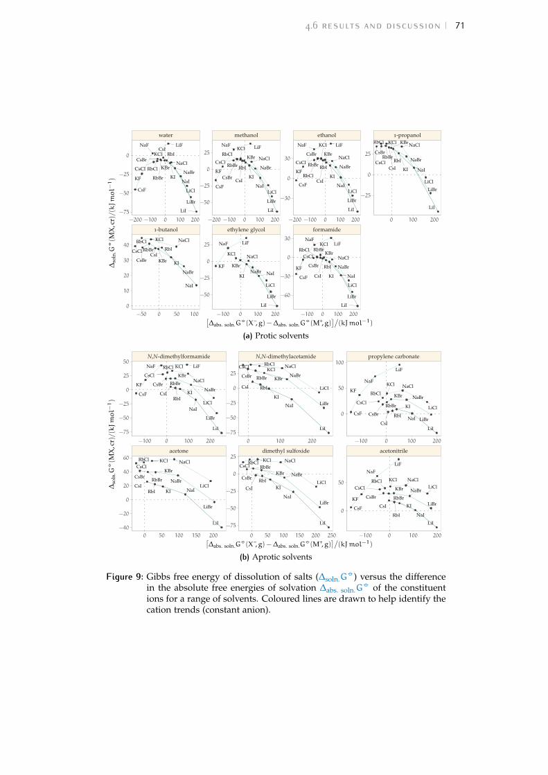
4.6 results and discussion 71
NaBr
NaCl
NaI
CsF
RbBr
LiBr
LiF
KI
KCl
KF
CsCl KBr
NaF
LiI
CsIRbI
CsBr
LiCl
RbCl
KCl
KIKBr
NaI
NaBr
RbI
CsBr
CsClCsI
RbBr
NaClRbCl
CsBr
RbCl
CsIKI
KBr NaCl
LiClNaI
KCl
LiI
LiF
NaBr
LiBr
RbBrKF
CsF
RbI
NaF
CsCl
NaCl
LiI
KBr
LiCl
KCl
KF
LiF
KI NaINaBr
NaF
LiBr
KFRbIRbBr
CsI
KBr
NaF
NaBr
KCl
CsBr
LiBr
KI
CsF
LiI
NaI
CsClNaCl
RbCl
LiF
LiCl
LiCl
RbBr
NaBr
NaI
NaF
CsF
LiBr
RbI
LiFRbCl
KI
LiI
CsI
CsBrKF
NaClKBr
CsCl
KCl
KCl
RbBr
CsICsCl
NaI
NaClKBr
LiCl
CsBr
NaBr
KI
LiI
RbCl
LiBr
RbI
1-butanol ethylene glycol formamide
water methanol ethanol 1-propanol
−50 0 50 100 −100 0 100 200 −100 0 100 200
−200 −100 0 100 200 −200 −100 0 100 200 −200 −100 0 100 200 0 100 200
−25
0
25
−30
0
30
−60
−30
0
30
−50
−25
0
25
−50
−25
0
25
−75
−50
−25
0
0
10
20
30
40
[∆abs. soln.G
−◦ (X–, g) −∆abs. soln.G−◦ (M+, g)
]/(kJmol−1)
∆so
ln.G
−◦(M
X,c
r)/(kJmol−
1)
(a) Protic solvents
KF
CsCl
CsF KI
NaILiCl
RbI
LiF
CsI
KBr
NaF RbCl KCl
CsBrNaCl
LiBr
RbBr
LiI
NaBr
RbCl
CsBr
LiI
LiBr
NaCl
LiClNaI
RbBr
CsClKBr
RbI
KCl
KI
NaBrCsI
NaCl
NaI
LiI
LiCl
RbCl
CsBr
CsI RbI
KILiBr
CsCl
KBr
KClNaBrRbBr
RbI
CsCl
LiI
LiBr
CsILiCl
NaClKCl
KBrRbBr
NaI
RbCl
CsBrNaBr
KI
RbI
NaCl
LiBr
NaF
KF
CsBr
KICsF
CsCl
LiF
NaI
NaBr
LiI
KBr
RbBr
KCl
CsI
LiCl
RbCl
KCl
NaF
KBrCsCl
CsI
NaBr
KI
LiCl
LiBr
NaCl
RbICsF
LiF
KF
NaI
LiI
RbBr
RbCl
CsBr
acetone dimethyl sulfoxide acetonitrile
N,N-dimethylformamide N,N-dimethylacetamide propylene carbonate
0 50 100 150 200 0 50 100 150 200 250 −100 0 100 200
−100 0 100 200 0 100 200 −100 0 100 200
0
50
100
0
50
−75
−50
−25
0
25
−75
−50
−25
0
25
−75
−50
−25
0
25
50
−40
−20
0
20
40
60
[∆abs. soln.G
−◦ (X–, g) −∆abs. soln.G−◦ (M+, g)
]/(kJmol−1)
∆so
ln.G
−◦(M
X,c
r)/(kJmol−
1)
(b) Aprotic solvents
Figure 9: Gibbs free energy of dissolution of salts (∆soln.G−◦ ) versus the difference
in the absolute free energies of solvation ∆abs. soln.G−◦ of the constituent
ions for a range of solvents. Coloured lines are drawn to help identify thecation trends (constant anion).

72 volcano plots
ity of anions in non-aqueous solvents, derived from their poor degree ofsolvation, (‘naked’ anions), is advantageous in several organic synthesis re-actions (Parker, 1962).
In contrast, whereas the anion trends for protic solvents also follow thevolcano trend (Appendix B, Figs. 74 and 76), the volcano shape is lost inaprotic solvents (see Appendix B, Figs. 75 and 77). As the data regardingfluoride salts are not available in aprotic solvents, it is not possible to observethe complete trend.
From these observations some general rules of thumb can be proposed.Firstly, the ion-specific trends observed in water are observed in protic sol-vents. Secondly, in aprotic solvents the ion-specific trends observed in waterare likely to hold for the cation trends (constant anion) but not for the anions(constant cation).
For anion trends in particular, it often happens that the electrolyte oc-cupying the peak position of the volcano changes, when changing from onesolvent to another. This has been reported by Arslanargin et al. (2016) inthe case of the dissolution enthalpies of the potassium fluoride–chloride–bromide series in water and pc: it increases from fluoride to bromide inwater, whereas it decreases from fluoride to bromide in pc. The larger dataset used here shows that the situation is complex across all solvents and suchbehaviour also happens in protic solvents (e.g. in proh).
The observed volcano shape for the enthalpies of dissolution of anionscan be justified as follows: in aprotic solvents, the enthalpy of dissolution ofanions gets less favourable (more endothermic, and therefore more positive)as the anion size decreases with respect to the cation size, because the dis-persion contributions to the ion-solvent interactions become smaller. An ‘ex-ploded’ volcano plot of enthalpies is shown in Figs. 69 and 70 of Appendix Bto facilitate the analysis of the single anion trends for different cations. Asanions are quite polarisable, the dispersion interactions play an importantrole in their solvation. This increasing dissolution enthalpy with decreasinganion size gives rise to the ‘right arm’ of the volcano. The solvation of the an-ion becomes more favourable only when specific bonding interactions withthe solvent, such as hydrogen bonds, intervene. These interactions are whatgives rise to the left slope of the volcano, which is not observed if the sol-vent is not capable of these interactions. Therefore, a true volcano shape isonly going to be observed for protic solvents, which have hydrogen bondingabilities and are therefore good anion solvators (Böes et al., 2006), or in caseswhere the solvent can form specific interactions with the anion.

4.7 interpretation of volcano plots in solvents 73
4.7 interpretation of volcano plots in solvents4.7.1 The origin of volcano plots
Some authors (Collins, 1997, 2004, 2006, 2012; Collins, Neilson et al., 2007;Morris, 1969; Schmidtchen, 2010) attribute the origin of the volcano trendto the interactions of the ions with the solvent, following the original ideaof Fajans’s competition principle (Fajans and Johnson, 1942). Other authorsinstead see it as a consequence of the properties of the ions alone, suchas size (Conway, 1977; Dzubiella et al., 2009). In an attempt to clarify thesituation, two tests are performed here.
Firstly, we can use the difference of the radii of the ions composing theelectrolyte in place of the difference of their absolute solvation energies. Ascan be seen in Figs. 10 and 11 (cation trends) and in Appendix B in Figs. 78to 81 (anion trends), the same volcano trend is obtained.
It must be highlighted here that the ionic radii used in the plots are thosefor the ions in water, as this is the only solvent for which estimates of thesolvated ion sizes are available. In a different solvent, these are likely to bedifferent, as they depend on the ion coordination number, which changesacross solvents (Marcus, 2016). But these aqueous radii correlate well withthe ab-initio radii calculated by Parsons and Ninham (2009) and they areavailable for a larger number of ions than the ab-initio radii. The aqueousradii values used provide an estimate that is sufficient for non-aqueous solv-ated ions, especially as the cation-anion difference has been used and itstrend can be expected to vary even less than the absolute values of the radiiitself. As the volcano shapes are retained when using the differences in theionic radii in place of the ionic solvation energies difference, the hypothesisthat it is the properties of the ions alone that give rise to the volcano trendappears equally valid. Moreover as the radii are a more fundamental charac-teristic, it can be argued that the radii are ultimately the origin of the volcanotrend. An argument that was proposed by Fajans and Johnson (1942) in fa-vour of solvation enthalpies rather than radii, is the fact that the maximumof the volcano occurs when the former is closer to zero. This was also usedto justify the ‘matching solvent affinity’ idea and the competition principleitself.
But the maximum is not at zero in all solvents represented in Fig. 9.In addition, the fact that the maxima occur at non-zero radii differences(Figs. 10 and 11) can be interpreted as a solvent-specific characteristic, as theregion of the solvent that most strongly interacts with the ion will differ forcations and anions (i.e., for a certain solvent with anion-solvating and cation-solvating groups of a certain size, ions will be best solvated when their sizedifference is closest to the difference in distances of solvation of the anion
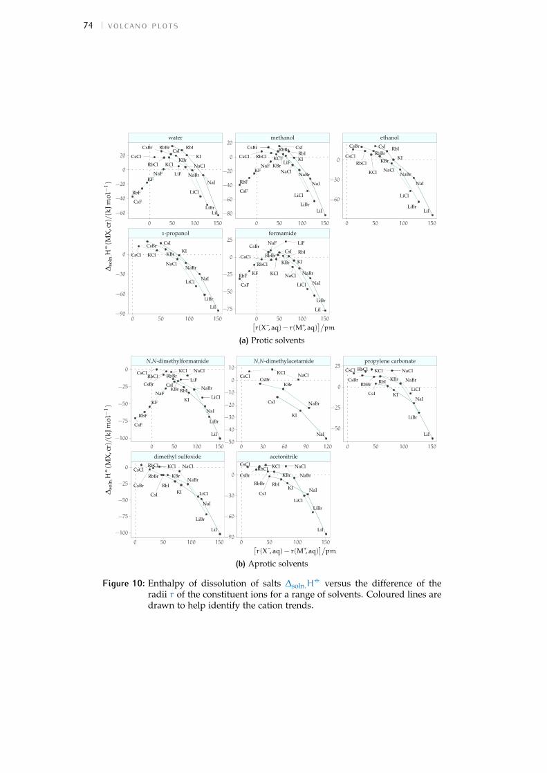
74 volcano plots
NaBr
NaCl
NaI
CsF
RbBr
LiBr
LiF
RbF
KI
KCl
KF
CsClKBr
NaF
LiI
CsIRbICsBr
LiCl
RbCl
KCl
CsI
CsCl
NaI
NaCl
KBr
LiCl
CsBr
NaBr
KI
LiI
LiBr
CsBr
RbCl
CsI
KIKBr
NaCl
LiCl
NaI
KCl
LiI
LiF
NaBr
LiBr
RbBr
RbF
KF
CsF
RbI
NaF
CsCl
LiCl
RbBr
NaBr
NaI
NaF
CsF
LiBr
RbI
RbF
LiF
RbCl KI
LiI
CsICsBr
KF NaCl
KBrCsCl
KCl
RbIRbBr
CsI
KBr
NaBrKCl
CsBr
LiBr
KI
LiI
NaI
CsCl
NaClRbCl
LiCl
1-propanol formamide
water methanol ethanol
0 50 100 150 0 50 100 150
0 50 100 150 0 50 100 150 0 50 100 150
−60
−30
0
−80
−60
−40
−20
0
20
−75
−50
−25
0
25
−60
−40
−20
0
20
−90
−60
−30
0
[r(X–, aq) − r(M+, aq)
]/pm
∆so
ln.H
−◦(M
X,c
r)/(kJmol−
1)
(a) Protic solvents
KF
RbF
CsCl
CsF
KI
NaI
LiClRbI
LiFCsI
KBrNaF
RbClKCl
CsBr
NaCl
LiBr
RbBr
LiI
NaBr
RbI
CsCl
LiI
LiBr
CsI LiCl
NaClKCl
KBrRbBr
NaI
RbCl
CsBrNaBr
KI
NaCl
NaI
CsBr
CsI
KI
CsCl
KBr
KCl
NaBr
KCl
KBr
CsCl
CsI
NaBr
KI
LiCl
LiBr
NaCl
RbINaI
LiI
RbBr
RbClCsBr
RbI
NaCl
LiBr
CsBr
KI
CsCl
NaI
NaBr
LiI
KBrRbBr
KCl
CsILiCl
RbCl
dimethyl sulfoxide acetonitrile
N,N-dimethylformamide N,N-dimethylacetamide propylene carbonate
0 50 100 150 0 50 100 150
0 50 100 150 0 30 60 90 120 0 50 100 150
−50
−25
0
25
−50
−40
−30
−20
−10
0
10
−90
−60
−30
0
−100
−75
−50
−25
0
−100
−75
−50
−25
0
[r(X–, aq) − r(M+, aq)
]/pm
∆so
ln.H
−◦(M
X,c
r)/(kJmol−
1)
(b) Aprotic solvents
Figure 10: Enthalpy of dissolution of salts ∆soln.H−◦ versus the difference of the
radii r of the constituent ions for a range of solvents. Coloured lines aredrawn to help identify the cation trends.
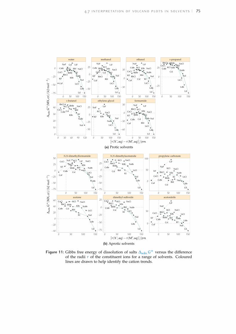
4.7 interpretation of volcano plots in solvents 75
NaBr
NaCl
NaI
CsF
RbBr
LiBr
LiF
KI
KCl
KF
CsCl
KBr
NaF
LiI
CsI
RbICsBr
LiCl
RbCl
KCl
KIKBr
NaI
NaBr
RbICsBr
CsClCsI
RbBr NaClRbCl
CsBr
RbCl
CsI KI
KBr NaCl
LiCl
NaI
KCl
LiI
LiF
NaBr
LiBr
RbBr
KF
CsFRbI
NaF
CsCl
NaCl
LiI
KBr
LiCl
KCl
KF
LiF
KINaI
NaBr
NaF
LiBr
KF RbIRbBr
CsI
KBr
NaF
NaBr
KClCsBr
LiBr
KICsF
LiI
NaI
CsClNaCl
RbCl
LiF
LiCl
LiCl
RbBr
NaBr NaI
NaF
CsF
LiBr
RbI
LiFRbCl
KI
LiI
CsICsBr
KF
NaClKBrCsClKCl
KCl
RbBr
CsI
CsCl
NaI
NaCl
KBr
LiCl
CsBrNaBr
KI
LiI
RbCl
LiBr
RbI
1-butanol ethylene glycol formamide
water methanol ethanol 1-propanol
0 30 60 90 120 0 50 100 150 0 50 100 150
0 50 100 150 0 50 100 150 0 50 100 150 0 50 100 150
−25
0
25
−30
0
30
−60
−30
0
30
−50
−25
0
25
−50
−25
0
25
−75
−50
−25
0
0
10
20
30
40
[r(X–, aq) − r(M+, aq)
]/pm
∆so
ln.G
−◦(M
X,c
r)/(kJmol−
1)
(a) Protic solvents
KF
CsCl
CsF
KI
NaI
LiCl
RbI
LiF
CsI
KBr
NaF
RbCl
KCl
CsBr
NaCl
LiBr
RbBr
LiI
NaBr
RbCl
CsBr
LiI
LiBr
NaCl
LiCl
NaI
RbBr
CsCl
KBr
RbI
KCl
KI
NaBrCsI
NaCl
NaI
LiI
LiCl
RbCl
CsBr
CsI RbIKI
LiBr
CsClKBr
KCl
NaBrRbBr
RbI
CsCl
LiI
LiBr
CsI LiCl
NaClKClKBr
RbBr
NaI
RbCl
CsBr NaBr
KI
RbI
NaCl
LiBr
NaF
KF
CsBr
KI
CsF
CsCl
LiF
NaI
NaBr
LiI
KBr
RbBr
KCl
CsI
LiCl
RbCl
KCl
NaF
KBrCsCl
CsI
NaBr
KI
LiCl
LiBr
NaCl
RbI
CsF
LiF
KF
NaI
LiI
RbBr
RbCl
CsBr
acetone dimethyl sulfoxide acetonitrile
N,N-dimethylformamide N,N-dimethylacetamide propylene carbonate
0 50 100 150 0 50 100 150 0 50 100 150
0 50 100 150 0 50 100 150 0 50 100 150
0
50
100
0
50
−75
−50
−25
0
25
−75
−50
−25
0
25
−75
−50
−25
0
25
50
−40
−20
0
20
40
60
[r(X–, aq) − r(M+, aq)
]/pm
∆so
ln.G
−◦(M
X,c
r)/(kJmol−
1)
(b) Aprotic solvents
Figure 11: Gibbs free energy of dissolution of salts ∆soln.G−◦ versus the difference
of the radii r of the constituent ions for a range of solvents. Colouredlines are drawn to help identify the cation trends.

76 volcano plots
and cation). The position of the maximum therefore reflects the asymmetryof the solvent molecules. This could be further tested by estimating thesolvated radii of ions in non-aqueous solvents.
A second test that can be made is to look at the trends for electrolytes con-taining polyatomic ions of different geometries: tetrahedral, such as ClO4
– ,trigonal planar (NO3
– ) and linear (SCN– ). For polyatomic ions the ion is notspherical, therefore the radius of the ion is a poorly defined measure. There-fore, for polyatomic ions, plots against the difference in radii of the anionand cation are less likely to show a volcano trend whereas plots against thedifferences in enthalpy or Gibbs free energy of solvation should still exhibit avolcano trend, if the origin of the volcano trend is truly the energetics of theinteraction of the ions with the solvent, as these measures remain reliable forpolyatomic ions. However, for polyatomic ions, volcano plots are generallynot observed, either when the solvation energies or the radii are used to con-struct the x-coordinate (abscissa). Exceptions are electrolytes containing ionswith tetrahedral geometry, such as perchlorates, which do show an extremalbehaviour that is in accordance with a volcano plot. Volcano plots of elec-trolytes containing an alkali metal cation and a polyatomic anion are shownin Figs. 12 to 15 (connecting lines highlighting cation trends). Although notall electrolytes are available, there is little evidence of a volcano trend inboth cases. For polyatomic ions volcano plots are not observed either whenthe solvation energies or the radii are used to construct the x-coordinate(abscissa).
The above two tests indicate that the radii hypothesis is preferable overthe solvation energies hypothesis, as they give equal results in terms of vol-cano plots, and the former is a simpler, more fundamental concept. Further,volcano trends are not observed for most salts containing polyatomic ions,whereas they would be expected under the solvation energies hypothesis.Finally and importantly, the solvation energies depend on the size of the ion.It is important to clarify here, that when I ascribe the effect to the ‘radius’ or‘size’ of the ion, all other properties of the ion that are convoluted with size(polarisability, etc.) are included. If the volcano plot can truly be ascribedto the ion alone, then it would be most interesting to acquire the solvatedradii of ions in non-aqueous solvents. Using these radii, an analysis of theposition of the maximum in volcano plots in different solvents might revealimportant details of solvation such as the distance of solvation of ions indifferent solvents and differences between cations and anions.
Details about the trends of polyatomic ions
Volcano plots of electrolytes containing polyatomic anions are shown inFigs. 12 to 15 (cation trends), and in Appendix B in Figs. 72 and 73 (cationtrends). The perchlorates show extremal behaviour and are therefore in

4.7 interpretation of volcano plots in solvents 77
LiNO3
NaOAc
NaForm
CsNO3 KClO4
RbClO4
KSCN
CsClO4
NaNO3
LiClO4
RbOAc
KNO3
NaClO4
NaSCN
RbNO3
KOAc
KForm
CsNO3
NaClO4
KClO4
RbClO4
KSCN
KNO3
NaSCNLiNO3
LiClO4
RbNO3
CsClO4
NaNO3
NaSCN
KSCN
KNO3
RbClO4
RbNO3
LiNO3
CsClO4
LiClO4
CsNO3
KClO4
NaClO4
NaNO3KSCN
NaSCN
NaSCN
LiClO4
KSCN
RbClO4
KClO4
CsClO4
NaClO4
NaSCN
CsClO4CsNO3
NaNO3
RbNO3
NaClO4
KSCN
RbClO4
LiClO4
KNO3
KClO4
LiNO3
CsClO4
LiClO4
NaClO4
KClO4
RbClO4
NaSCN
KSCN
NaClO4
KClO4
CsClO4
KNO3CsNO3
LiClO4
NaSCNLiNO3
NaNO3RbNO3
RbClO4
CsClO4
NaClO4
KSCNKClO4
propylene carbonate dimethyl sulfoxide acetonitrile
formamide N,N-dimethylformamide N,N-dimethylacetamide
water methanol ethanol
−100 0 100 200 300 −100 0 100 200 300 −100 0 100 200 300
−50
−25
0
25
−40
−30
−20
−10
0
−60
−40
−20
0
20
−40
−20
0
20
−60
−40
−20
0
−60
−40
−20
0
−20
0
20
40
60
−60
−40
−20
0
20
−20
−15
−10
−5
0
[∆abs. soln.H
−◦ (X–, g) −∆abs. soln.H−◦ (M+, g)
]/(kJmol−1)
∆so
ln.H
−◦(M
X,c
r)/(kJmol−
1)
Figure 12: Salts containing polyatomic anions. Enthalpy of dissolution ∆soln.H−◦
versus the difference in the absolute enthalpies of solvation of the con-stituent ions ∆abs. soln.H
−◦ . Coloured lines are drawn to help identify thecation trends.

78 volcano plots
LiNO3NaOAc
NaForm
CsNO3KClO4RbClO4
KSCN
CsClO4
NaNO3
LiClO4
KNO3
NaClO4
RbNO3
NaClO4
RbClO4
LiClO4
CsClO4 KClO4
LiClO4
KSCN
RbClO4
KClO4
NaOAc
CsClO4
NaClO4
KNO3CsNO3
LiClO4
LiNO3NaNO3
RbNO3 RbClO4
CsClO4
NaClO4
NaOAc
KSCN
KClO4
KNO3
RbClO4
RbNO3
LiNO3
CsClO4
LiClO4
NaOAc
CsNO3KClO4
NaClO4
NaNO3
KSCN
CsClO4
NaClO4
RbClO4
KClO4
RbClO4KClO4
LiClO4
KSCN
NaClO4
CsClO4
CsClO4
CsNO3
KSCN
NaNO3
LiClO4
KNO3
NaOAc
RbNO3
NaClO4
KClO4
LiNO3
RbClO4
NaClO4
KClO4
RbClO4
KSCN
LiClO4
CsClO4
NaOAc
CsClO4
NaOAc
NaClO4
KSCN
RbClO4
LiClO4
KClO4
acetonitrile
N,N-dimethylformamide propylene carbonate dimethyl sulfoxide
1-propanol 1-butanol formamide
water methanol ethanol
0 100 200 300
0 100 200 300 0 100 200 300
−20
0
20
40
−60
−40
−20
0
−50
−25
0
−40
−20
0
20
0
20
40
60
−20
−10
0
10
−40
−20
0
−20
0
20
40
−50
−25
0
25
−20
0
20
40
[∆abs. soln.G
−◦ (X–, g) −∆abs. soln.G−◦ (M+, g)
]/(kJmol−1)
∆so
ln.G
−◦(M
X,c
r)/(kJmol−
1)
Figure 13: Salts containing polyatomic anions. Gibbs free energy of dissolution∆soln.G
−◦ versus the difference in the absolute Gibbs free energies ofsolvation of the constituent ions ∆abs. soln.G
−◦ . Coloured lines are drawnto help identify the cation trends.
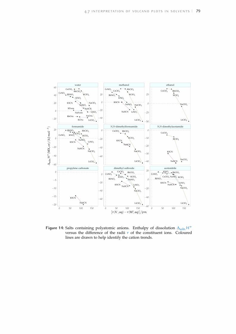
4.7 interpretation of volcano plots in solvents 79
LiNO3
NaOAc
NaForm
CsNO3 KClO4
RbClO4
KSCN
CsClO4
NaNO3
LiClO4
RbOAc
KNO3
NaClO4
NaSCN
RbNO3
KOAc
KForm
CsNO3
NaClO4
KClO4
RbClO4
KSCN
KNO3
NaSCN
LiNO3
LiClO4
RbNO3
CsClO4
NaNO3
NaSCN
KSCN
KNO3
RbClO4
RbNO3
LiNO3
CsClO4
LiClO4
CsNO3
KClO4
NaClO4NaNO3
KSCN
NaSCN
NaSCN
LiClO4
KSCN
RbClO4
KClO4
CsClO4
NaClO4
NaSCN
CsClO4CsNO3
NaNO3RbNO3
NaClO4
KSCN
RbClO4
LiClO4
KNO3 KClO4
LiNO3
CsClO4
LiClO4
NaClO4
KClO4
RbClO4
NaSCN
KSCN
NaClO4
KClO4
CsClO4
KNO3CsNO3
LiClO4
NaSCNLiNO3
NaNO3RbNO3
RbClO4
CsClO4
NaClO4
KSCN
KClO4
propylene carbonate dimethyl sulfoxide acetonitrile
formamide N,N-dimethylformamide N,N-dimethylacetamide
water methanol ethanol
0 50 100 150 0 50 100 150 0 50 100 150
−50
−25
0
25
−40
−30
−20
−10
0
−60
−40
−20
0
20
−40
−20
0
20
−60
−40
−20
0
−60
−40
−20
0
−20
0
20
40
60
−60
−40
−20
0
20
−20
−15
−10
−5
0
[r(X–, aq) − r(M+, aq)
]/pm
∆so
ln.H
−◦(M
X,c
r)/(kJmol−
1)
Figure 14: Salts containing polyatomic anions. Enthalpy of dissolution ∆soln.H−◦
versus the difference of the radii r of the constituent ions. Colouredlines are drawn to help identify the cation trends.
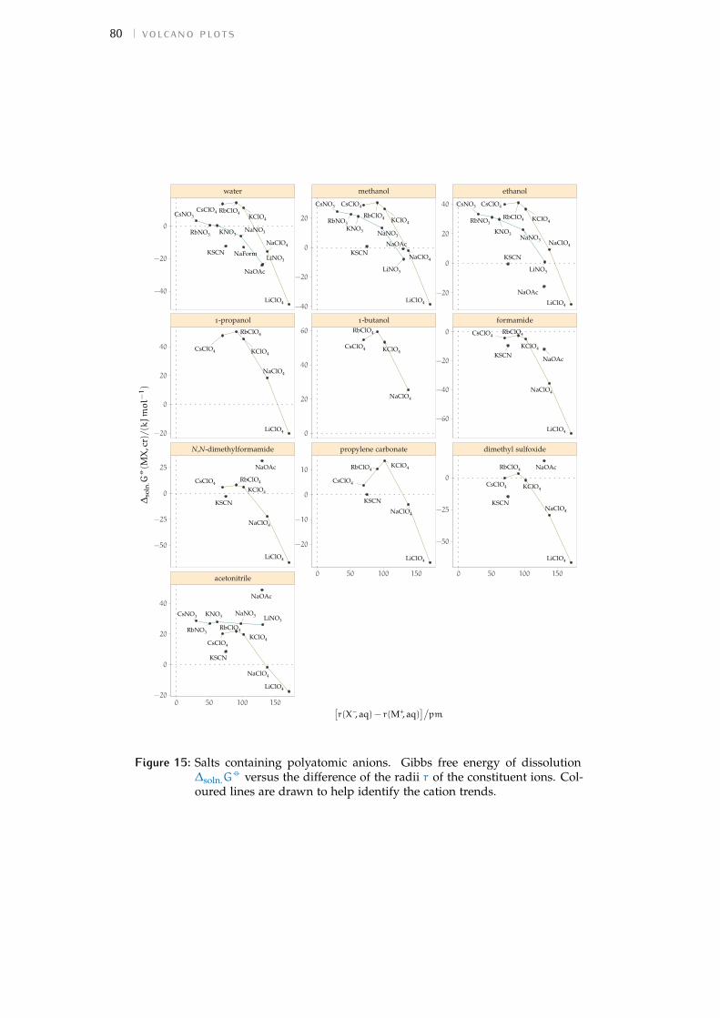
80 volcano plots
LiNO3
NaOAc
NaForm
CsNO3 KClO4
RbClO4
KSCN
CsClO4
NaNO3
LiClO4
KNO3
NaClO4
RbNO3
NaClO4
RbClO4
LiClO4
CsClO4 KClO4
LiClO4
KSCN
RbClO4
KClO4
NaOAc
CsClO4
NaClO4
KNO3CsNO3
LiClO4
LiNO3NaNO3
RbNO3RbClO4
CsClO4
NaClO4
NaOAc
KSCN
KClO4
KNO3
RbClO4RbNO3
LiNO3
CsClO4
LiClO4
NaOAc
CsNO3
KClO4
NaClO4
NaNO3
KSCN
CsClO4
NaClO4
RbClO4
KClO4
RbClO4 KClO4
LiClO4
KSCN
NaClO4
CsClO4
CsClO4CsNO3
KSCN
NaNO3
LiClO4
KNO3
NaOAc
RbNO3
NaClO4
KClO4
LiNO3
RbClO4
NaClO4
KClO4
RbClO4
KSCN
LiClO4
CsClO4
NaOAc
CsClO4
NaOAc
NaClO4KSCN
RbClO4
LiClO4
KClO4
acetonitrile
N,N-dimethylformamide propylene carbonate dimethyl sulfoxide
1-propanol 1-butanol formamide
water methanol ethanol
0 50 100 150
0 50 100 150 0 50 100 150
−20
0
20
40
−60
−40
−20
0
−50
−25
0
−40
−20
0
20
0
20
40
60
−20
−10
0
10
−40
−20
0
−20
0
20
40
−50
−25
0
25
−20
0
20
40
[r(X–, aq) − r(M+, aq)
]/pm
∆so
ln.G
−◦(M
X,c
r)/(kJmol−
1)
Figure 15: Salts containing polyatomic anions. Gibbs free energy of dissolution∆soln.G
−◦ versus the difference of the radii r of the constituent ions. Col-oured lines are drawn to help identify the cation trends.

4.8 volcano plots in the ‘real world’ 81
agreement with a volcano trend. The maximum for these series is not posi-tioned close to a zero x-value as occurs in the classic volcano plots of alkalimetal halides, but is shifted towards positive values. Plots against the dif-ference in solvation energies and against the difference in radii show thesame trend, thus indicating no preferential dependence of the volcano onsolvation energies rather than radii. For thiocyanates, formates and acetatestoo little data is available to make an assessment, but the data is plotted forcompleteness.
4.7.2 Consequences
As espoused in Section 4.6.3, the existence of volcano plots in other solventsinfers that, across solvents, the ion-specific trends observed in water will beobserved in other protic non-aqueous solvents, and that the trends observedin water are more likely to hold for cations in non-aqueous solvents than foranions. This is a very interesting piece of information, which poses questionsabout the role of the solvent properties (hydrogen bonding, polarisability) inanion solvation. The trends in standard solution thermodynamic quantitiesbehave differently than the electrostriction trends discussed in Chapter 3,despite both being bulk properties of solutions. For electrostrictive volumes,we have seen that both cations and anions follow the same ion-specific seriesacross all solvents. Here, the homogeneity in ion-specific behaviour holds forcations in protic and aprotic solvents and anions in protic solvents, but notfor anions in aprotic solvents. How do the two results reconcile? Despitesolution energies and electrostrictive volumes being both bulk propertiesat standard concentration, they are very different in nature, with the firstbeing more sensitive to ion-solvent specific interactions. This also showsthat experiments can probe different aspects of ion-solvent interaction, andtherefore the series observed can reveal different details of solvation.
This information is also useful in terms of predicting the unknown ion-specific trends in non-aqueous solvents where the corresponding trends areknown in water. It must be stressed here, that all of the above analysis andobservations are valid for standard, bulk quantities. I explore whether thisholds at real concentrations below.
4.8 volcano plots in the ‘real world’As stated in Section 4.5.2, in the lmwa foundations standard thermody-namic quantities were used to explain electrolyte behaviour at finite concen-trations. The use of ion-ion interactions arguments to explain data at infinitedilution is not justified, as the activity of a species at infinite dilution is by

82 volcano plots
definition 1, and therefore ion pairing is excluded. Despite this, the lmwaholds very well in water and explains a number of phenomena that occurin solution at finite concentrations of electrolyte (and often in very complexsystems, where surfaces, macromolecules, high concentrations and so onare present). The quantities analysed so far contain no information aboutthe behaviour of ions at real concentrations (but still they are useful in in-forming the ion-solvent interactions in non-aqueous solvents!). An attemptat investigating the volcano trends at finite concentrations in water and non-aqueous solvents is therefore made here, by considering the solubility andactivity coefficients of electrolytes in non-aqueous solvents. The ultimategoal is to test whether volcano plots are evident in these systems and thelmwa reasoning (or the theory proposed by Ninham and collaborators) canbe extended to non-aqueous solvents.
4.8.1 The solubility of electrolytes
In order to ascertain if a volcano trend is exhibited in the solubility S of elec-trolytes, the molal solubilities of alkali metal halides against the differenceof their radii are plotted in Figs. 84 and 85 of Appendix B.
A reversed volcano plot is observed in water, and, despite the scarce avail-ability of information, it is retained in meoh and the homologous series ofalcohols, although the solubility decreases rapidly along the series (the dataare therefore plotted using a semi-logscale). Also, there is a suggestion of aninverted volcano trend in the other protic non-aqueous solvents. In aproticsolvents, the left slope of the inverted volcano is missing. That is, where thefluorides series and chloride series are present, their solubility does not in-crease going towards smaller x-values. This is interesting and confirms whatwas observed previously in regards to the solvation of anions by aprotic sol-vents: it does not matter how much the ions are ‘mismatched’, the solvationof the fluoride and chloride anions in aprotic solvents is so unfavourablethat the solubility of their salts is very low. This also demonstrates thatthe thermodynamics of the volcano plots at infinite dilution is not directlyconnected to the electrolyte solubility. This is also shown by the fact that,whereas the trend of KF – KCl – KBr dissolution energies observed in wateris the opposite of the trend in pc (Arslanargin et al., 2016), the solubilities inthe two solvents follow unrelated trends: KCl < KBr < KF < KI in water, andKF < KCl < KBr < KI in pc.
4.8.2 Activity coefficients
Activity coefficients γ are the ideal quantifier for ion-ion interactions in solu-tion. For this analysis, I have also collected the activity and osmotic coef-

4.8 volcano plots in the ‘real world’ 83
CsBrCsCl
CsF
CsI
KBrKCl
KFKI
LiBrLiCl
LiI
NaBrNaCl
NaF
NaI
RbBr
RbCl
RbF
RbI
CsBr
CsCl CsI
KBrKClKI
LiBr
LiCl
NaBr
NaCl
NaI
CsI
KBrKI
LiBr
NaBrNaCl
NaIRbI
KI
LiBr
LiI
NaI
LiBr
LiClLiI
NaI
CsI
KI
NaI
CsCl
KCl
LiCl
NaBr
NaCl
CsI
KI
LiBr
LiCl
NaCl
NaI
RbI
N-methylacetamide propylene carbonate ethylene carbonate dimethyl sulfoxide
water methanol ethanol N-methylformamide
0 50 100 0 50 100 150 0 30 60 90 120 0 50 100
0 50 100 150 0 50 100 0 50 100 150 0 30 60 90
0.850
0.875
0.900
0.925
0.5
0.6
0.7
0.8
0.200
0.225
0.250
0.275
0.84
0.86
0.88
0.90
0.50
0.55
0.60
0.65
0.70
0.60
0.65
0.70
0.75
0.65
0.70
0.75
0.80
0.94
0.96
0.98
1.00
[r(X–, aq) − r(M+, aq)
]/pm
γ±
mea
nac
tivi
tyco
effic
ient
Figure 16: Inverted volcano plots of the activity coefficients γ versus the differenceof the radii r of the constituent ions. The electrolyte concentration is0.4mol kg−1, except for: meoh (0.07mol kg−1); pc (0.18mol kg−1); ecand nma, (0.09mol kg−1); dmso and nmf (0.05mol kg−1). Colouredlines are drawn to help identify the cation trends.
ficients available in the literature for non-aqueous solvents. The data havebeen fitted (where no fitting was performed in the original paper) in orderto interpolate to an intermediate concentration value so that as many elec-trolytes as possible can be compared. Unfortunately, the data available fornon-aqueous solvents is scarce.
Plots of the activity coefficients plotted versus the ionic radii differenceare shown in Fig. 16 (Fig. 83 in Appendix B highlights the anion trends).The osmotic coefficients are shown in Appendix B, Fig. 71 (lines highlightingcation trends), and Fig. 82 (lines following anion trends). In addition, Figs. 72and 73 show the plots for electrolytes containing a polyatomic anion.
It is important to clarify that the coefficients plotted for each solvent arefor a specific salt concentration, which is not preserved across solvents dueto different electrolyte solubility.
For alkali metal halides in water, we observe the inverted volcano as pro-posed by Duignan (with Bromley’s B-coefficients) and mentioned by Fajansand Soniat et al. (2016). This same trend seems to show in meoh, N-methylacetamide (nma), dmso and in ec (although just three points areavailable in this solvent). The trend in nmf is reversed. This is interestingbecause a reversal of the trend in nmf with respect to the other solvents isalso observed for the viscosity B-coefficient (vbc) of the alkali metal cationsseries (Table 13).
The scarcity of data is problematic, but the trends observed in water seemto be respected. The lack of data does not allow any conclusions to bedrawn regarding the differences between protic and aprotic solvents. It

84 volcano plots
seems though, that the ‘lmsa’ as proposed by Long et al. (2013) can besubstantiated in these non-aqueous solvents, except for nmf.
For electrolytes containing polyatomic anions, the data are too scarce toallow for any consideration, but they are nonetheless shown for complete-ness.
4.9 conclusionsThis analysis of volcano plots in solvents delivers a number of interestingdetails.
Firstly, the volcano plots of Morris are observed to be valid across proticand aprotic solvents, with the same trends as in water, with the exception ofanion trends in aprotic solvents.
Secondly, it is argued that fundamentally the volcano trends arise fromion size, and this also gives rise to the solvent affinity.
Thirdly, it is demonstrated that volcano trends are manifest not only understandard conditions of infinite dilution but also at real concentrations.
The work presented above is consistent with the following interpretation:ions, or charged moieties in any solvent, form ion pairs that are in closecontact when their size difference is most similar to the size difference ofthe cation- and anion-solvating groups of that solvent. The opposite is thecase for ions of different sizes, that are poorly associated and retain theirsolvation shells. This is valid for anions and cations in water and proticsolvents, and for cations that share the same anion in aprotic solvents. Thisis not strictly valid when comparing anions that share a common cation inaprotic solvents. Putting this last category aside, where the particulars ofthe solvation of the anions is more strongly solvent-specific and dominates,the formulation of a more general principle for the interaction of electrolytesin solvents that further develops the lmwa to encompass all solvents canbe proposed: sie are dominated by, and largely originate from, the relat-ive effective size of the anion and cation. The effective size being the sizeof the ion and the distance of closest approach of the solvating group. Thematching of effective ion size (meis) is therefore a useful and important gen-eral concept in understanding and predicting ion-specificity across solvents.That is, when the effective ion size of the cation and anion are matched, theions lose part of their solvation shell to associate in solution, whereas whenthe effective ion size of the cation and anion are mismatched the ions do notassociate. From this analysis the sie cannot be pinned to a single propertyof the ion, as it is impossible to deconvolve the effect of size, electrostaticcharge, polarisability, instantaneous dipoles (dispersion). Despite that, it isstriking that the volcano trend is maintained across solvents. The presence

4.9 conclusions 85
of common trends across solvents has been noted on occasion before, forinstance, in Criss and Mastroianni (1971), who, by analysing the cationic vis-cosity B-coefficient in water, meoh and mecn, also inferred that water isnot a different solvent in its interactions with ions. However, further experi-mental work is required in order to determine the specificity of the solventinfluence at finite concentrations.
These observations demonstrate that, as noted in Chapters 2 and 3 already,water is not a special solvent with respect to sie, in that non-aqueous sol-vents exhibit similar phenomena.
Theoretical work is needed in order to understand the details of ion-solvent interactions and explain the qualitative trends presented here, andultimately to develop a quantitative predictive theory of sie that appliesacross multiple solvents.


5 E X P E R I M E N TA L P R O C E D U R E S
This chapter summarises all the shared methodologies and materials thathave been used for the experiments performed. Also the general experi-mental problems associated with working with non-aqueous electrolytes arediscussed.
Most of the material is reproduced with minor changes from:
V. Mazzini, G. Liu et al. (2018), ‘Probing the Hofmeister Series beyond Wa-ter: Specific-ion Effects in Non-aqueous Solvents’, J. Chem. Phys. 148, 22,p. 222805, doi: 10.1063/1.5017278.
5.1 experimental materials5.1.1 Electrolytes
The experimental part of this thesis focuses on monovalent 1 : 1 electrolytesas in previous chapters, but the selection of electrolytes has been restricted toonly the sodium salts. Therefore these experiments are probing specific-anioneffects.
The reason for this choice is primarily practical. The aim is to test differ-ent solvents and therefore only a limited number of salts can be tested inorder for the measurements to be completed in a timely manner. In water,anions induce the most marked differences in the magnitude of sie. The as-sumption that this would hold for non-aqueous solvents as well is soundlygrounded, as the physical characteristics of the ions are not changing. Theseven anions considered are listed below according to their Hofmeister or-dering:
CH3COO− > F− > Cl− > Br− > I− > ClO4− > SCN−
The common cation is Na+. Molecular models of the salts and solvents areshown in Fig. 17.
Preparation of electrolytes — drying
The electrolytes were already available, and their specifications are listedin Table 21. The salts were used to prepare the samples without any furtherpurification beyond drying, which was performed periodically. Preliminary
87

88 experimental procedures
Table 21: Chemical specifications of the electrolytes used in the experiments.
electrolyte supplier product number specifications
NaOAc sigma® S− 3272 electrophoresis reagent > 99%NaF Ajax Chemicals 1230− 500G Univar® conforms to acsNaCl sigma-aldrich® S7653− 5KG BioXtra, > 99.5% (AT)NaBr Riedel-de Haën 02119 extra pure, Ph. Eur.NaI merck® 106523 acs reagent, Ph. Eur., > 99.5%NaClO4 sigma® 410241− 500G acs reagent, 98+ %NaSCN aldrich® 251410− 500G acs reagent, > 98%
Table 22: Oven drying protocol for the electrolytes.
electrolyte oven type t/◦C time/h
NaOAc vacuum 120 10NaF furnace 130 24NaCl furnace 130 24NaBr vacuum 140 12NaI vacuum 70 12NaClO4 vacuum 140 12NaSCN vacuum 120 12
experimental tests were performed with the salts as they were, without dry-ing.
The drying procedure was performed either in a furnace or in a vacuumoven, and a chemicals purification handbook (Armarego and Chai, 2009)was consulted for the recommended drying temperatures. Each salt wastransferred into a small Petri dish (diameter 4 cm), and the Petri dish wasplaced in the oven with the lid ajar. Clumps were broken with a mor-tar and pestle before being transferred to the Petri dish where needed, aswas the case for highly hygroscopic salts. The drying conditions are listedin Table 22 for each of the salts. After drying, the salts were quickly trans-ferred into dry 40ml glass vials equipped with polypropylene caps that hadbeen washed repeatedly with Type I ultrapure water (according to the ASTMD1193− 06 standard, produced with an ELGA PURELAB® Chorus I appar-atus) and dried overnight in an oven at 80 ◦C. The vial was allowed to coolin a desiccator over silica gel and under vacuum before placing the driedsalt inside. A piece of folded weighing paper, flushed with dry nitrogen,was used as a funnel for the transfer to the dry vial. After filling, a stripof Parafilm M® film was applied around the vial cap, and all the vials werethen stored in a desiccator over silica gel. The NaSCN and NaI vials werealso wrapped in aluminium foil in order to prevent light degradation. Thehygroscopic salts were dried periodically as required.

5.1 experimental materials 89
salts solventsmonoatomic
anionpolyatomic
anionhydrogenbonding
not hydrogenbonding
sodium fluoride
sodium chloride
sodium bromide
sodium iodide
sodium acetate
sodium thiocyanate
sodium perclorate
methanol
formamide
dimethyl sulfoxide
propylene carbonate
Figure 17: Stick-and-ball molecular models of the experiments salts and solvents.
A short digression on hygroscopicity
I deem it interesting to report the following observation. Sodium salts of‘kosmotropic’ anions, which are the ones that are strongly hydrated in aque-ous solution, are not hygroscopic at all. The powdered sodium salts of ‘chao-tropic’ anions, are instead progressively more hygroscopic going down theHofmeister series, to the point that NaSCN is a deliquescent salt. This iscounter-intuitive as one would expect the opposite. The reason for this isthat the crystal lattice free energy has to be taken into consideration, andthis is much larger for ‘matched’ ions such as Na+ and F– than for ‘mis-matched’ ones. This free energy follows Collins’ lmwa (Collins, 1997), dis-cussed in Section 4.4.
5.1.2 Solvents
In selecting the solvents to use, it was decided to experiment on two repres-entatives from each class of hydrogen-bonding capability (protic/aprotic).The reason for choosing two aprotic and two protic solvents, rather thantwo high permittivity or low permittivity ones for instance, is that hydrogenbonding abilities have been indicated as one of the fundamental enablers ofsie (Thomas and Elcock, 2007). As the present work is ultimately investigat-ing the origin of sie, it is important to explore this connection.
We have seen in the previous chapters that proticity does not matter ata fundamental level on sie. With this in mind, it is important to ascertainwhat happens when the system complexity increases with the addition of in-teracting surfaces and higher concentrations. Does proticity matter in thesenon-bulk, non-ideal conditions?

90 experimental procedures
Table 23: Technical specifications of the solvents investigated.
solvent supplier product number specifications
meoh rci Labscan Limited AH1118−G2.5L anhydrous, water max.50 ppm
fa sigma-aldrich® 47670− 1L− F puriss. p.a., acs reagent,> 99.5,%, 6 0.1% water, 60.02% free acid (HCOOH)
Fluka® 34724− 1L− R hydranal®, water max.200 ppm
dmso sigma-aldrich® 276855− 2L anhydrous, > 99.9%pc sigma-aldrich® 310328− 2L anhydrous, 99.7%
For the above reasons, the solvents chosen are meoh and fa as protic rep-resentatives, and dmso and pc as aprotic ones. The experiments have alsobeen performed in water in order to have a comparison. The physical prop-erties that these solvents span are very diverse, as Table 2 shows; molecularmodels representations of the salts and solvents are shown in Fig. 17.
Preparation
High purity, anhydrous solvents were purchased in order to avoid complica-tions with drying the solvents in-situ. In fact, tests in the drying of solventswith 3Å molecular sieves revealed that the solvent conductivity often in-creases upon the addition of molecular sieves (especially for meoh). Anincrease in conductivity means that ions (of unknown species) have beenreleased into the solvent. These ions represent an undesired contaminationthat could interfere with the effects of the ions of interest. Therefore theaddition of molecular sieves for drying the solvent, or for keeping the sol-vent dry was obviated. The water content was periodically checked throughKarl Fischer (kf) titration. The technical specifications of the solvents arethe description of the
technique isin Section 5.3.1,
page 95.
reported in Table 23. Preliminary tests were often carried out with non-drysolvent from bottles already available in the laboratory. It seems that smallquantities of water do not affect the sie trends, as no differences in the or-dering of ion effects were observed between experiments performed withstandard solvents and those performed with anhydrous solvents.
5.2 preparation of the salt solutionsThe electrolyte solutions were prepared in molality m (molkg−1) concen-tration units. Molality was preferred over concentration c in moldm−3 be-cause the solution density changes with the salt present (see Fig. 99 in Ap-pendix G), and this effect is relatively more significant at lower salt concen-

5.2 preparation of the salt solutions 91
trations. As the preparation of solutions by molality involves weighing bothsolute and solvent, it does not present the above mentioned complication.
A kern® ABJ− 220− 4M analytical balance was therefore used. A Petridish was employed as support for the vial and to distribute its weight on alarger surface of the balance plate. The vials where the solutions were goingto be prepared were washed with Type I ultrapure water, dried in an ovenovernight and kept in a plastic desiccator over silica gel and under vacuumbefore use. Typically 20 g to 25 g of solution (depending on its density) wereprepared each time in a 25ml vial. This quantity was preferred over largerquantities in order to facilitate storage in desiccators. Also, to avoid prob-lems associated with storage (e.g. contamination, evaporation of the solvent),it was preferred to re-prepare the solution more often rather than storing itfor a long time.
The salt was first weighed directly into the vial, followed by the addition ofthe solvent (as close as possible to the desired weight). Both salt and solventweight were noted in order to calculate the solution concentration with themaximum accuracy achievable. The weighing procedure was performed inair, as quickly as possible. The usage of a glove bag was considered andtrialled but the problems associated with the scale instability overcame theadvantage of weighing in a dry atmosphere. The relative humidity in thelaboratory was on average low (around 25%), therefore swift operation andthe monitoring of water content through Karl Fischer (kf) titration werepreferred for practicality.
Parafilm M® was applied around the vial cap immediately after prepar-ation to help prevent moisture ingress. When dissolution was not instant-aneous, a vortex mixer and sonication were used to help the dissolutionprocess. In some cases, such as for iodide salts, sonication was applied onlybriefly to avoid oxidation of the iodide to iodine (revealed by the appearanceof a yellow colour). This is particularly true for dmso solutions of NaI: nosonication was applied at all in this case.
5.2.1 Solubility of the salts
The solubility of the electrolytes in the different solvents is listed in Table 24.Most of the information was available in the literature. A salt concentra-tion that was accessible for most electrolytes in the different solvents is0.05mol kg−1. Therefore this was set as the electrolyte concentration for thechromatography experiments. Qcm measurements were performed withelectrolyte solutions of 10−3molkg−1 concentration. This lower concentra-tion was sufficient to produce detectable changes in the polymer brush be-haviour, whilst higher concentrations had little effect on the magnitude ofthe changes observed (see Fig. 29 in Chapter 7).
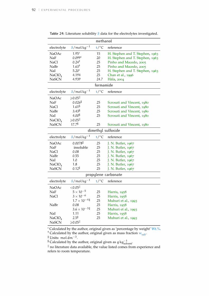
92 experimental procedures
Table 24: Literature solubility S data for the electrolytes investigated.
methanolelectrolyte S/molkg−1 t/◦C reference
NaOAc 1.95* 15 H. Stephen and T. Stephen, 1963NaF 0.099* 20 H. Stephen and T. Stephen, 1963NaCl 0.24† 25 Pinho and Macedo, 2005NaBr 1.63† 25 Pinho and Macedo, 2005NaI 5.20* 25 H. Stephen and T. Stephen, 1963NaClO4 4.194 25 Chan et al., 1996NaSCN 4.939 24.7 Hála, 2004
formamideelectrolyte S/molkg−1 t/◦C reference
NaOAc >0.05‖
NaF 0.026‡ 25 Scrosati and Vincent, 1980NaCl 1.61§ 25 Scrosati and Vincent, 1980NaBr 3.43§ 25 Scrosati and Vincent, 1980NaI 4.00§ 25 Scrosati and Vincent, 1980NaClO4 >0.05‖
NaSCN 17.7§ 25 Scrosati and Vincent, 1980
dimethyl sulfoxideelectrolyte S/molkg−1 t/◦C reference
NaOAc 0.0078‡ 25 J. N. Butler, 1967NaF insoluble 25 J. N. Butler, 1967NaCl 0.08 25 J. N. Butler, 1967NaBr 0.55 25 J. N. Butler, 1967NaI 1.0 25 J. N. Butler, 1967NaClO4 1.8 25 J. N. Butler, 1967NaSCN 0.12‡ 25 J. N. Butler, 1967
propylene carbonateelectrolyte S/molkg−1 t/◦C reference
NaOAc <0.05‖
NaF 5× 10⁻⁵ 25 Harris, 1958NaCl 3× 10⁻⁶ 25 Harris, 1958
1.7× 10⁻⁴‡ 25 Muhuri et al., 1993NaBr 0.08 25 Harris, 1958
3.6× 10⁻³‡ 25 Muhuri et al., 1993NaI 1.11 25 Harris, 1958NaClO4 2.5‡ 25 Muhuri et al., 1993NaSCN >0.05‖
* Calculated by the author, original given as ‘percentage by weight’ Wt.%.† Calculated by the author, original given as mass fraction wsalt.‡ Units: moldm−3.§ Calculated by the author, original given as gkg−1solvent.‖ no literature data available, the value listed comes from experience andrefers to room temperature.

5.3 the influence of trace quantities of water 93
Table 25: Summary of the electrolytes investigated per solvent.
electrolyte meoh fa dmso pc
NaOAc X XNaF XNaCl X X XNaBr X X XNaI X X X XNaClO4 X X X XNaSCN X X X X
The electrolytes investigated for each solvent are summarised in Table 25.Although there are literature reports (Harris, 1958) that NaBr is soluble inpc at a concentration of 5× 10⁻²molkg−1, it was not possible to achieveits solubilisation at that concentration nor at the lesser concentration of10−3molkg−1. Note the solubility of salts varies greatly across solventsand is in most cases lower than in water. This limits the range of electrolytesand the concentrations available for investigation.
5.2.2 Storage of solutions
The iodine and thiocyanate solutions vials were covered in aluminium foilto prevent light degradation of the anions. All the vials containing solutionswere kept in a glass desiccator over silica gel and granular phosphorouspentoxide, P4O10, which were changed regularly. Additionally, the desic-cator was placed under a slight vacuum.
5.3 the influence of trace quantities of waterWhen investigating sie in polar non-aqueous solvents, which are to someextent hygroscopic, the possible interference of water is a concern. It isknown that water can selectively solvate ions in mixtures with non-aqueoussolvents (J. N. Butler et al., 1971). Preferential solvation is found to be negli-gible for mixtures of solvents of similar polarity and/or hydrogen-bondingcapability (Marcus, 2004), therefore we can expect trace concentrations of wa-ter in meoh and fa to be distributed randomly in solution and within thesolvation shells of the ions. In the case of solvents that differ in polarity orhydrogen-bonding properties to water, such as dmso and pc, water prefer-entially solvates the anions, while the cations exhibit little to no preferentialsolvation (Marcus, 2005). This matters particularly for the experiments inthis work as they are probing specific-anion effects.
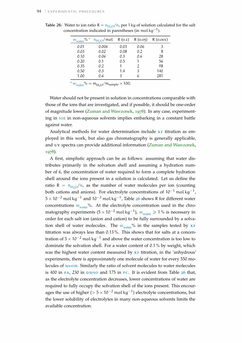
94 experimental procedures
Table 26: Water to ion ratio R = nH2O/ni per 1 kg of solution calculated for the saltconcentration indicated in parentheses (in molkg−1).
wwater% * nH2O/mol R (0.1) R (0.05) R (0.001)
0.01 0.006 0.03 0.06 30.03 0.02 0.08 0.2 80.10 0.06 0.3 0.6 280.20 0.1 0.5 1 560.35 0.2 1 2 980.50 0.3 1.4 3 1401.00 0.6 3 6 281
* wwater% = mH2O/msample × 100;
Water should not be present in solution in concentrations comparable withthose of the ions that are investigated, and if possible, it should be one-orderof magnitude lower (Zuman and Wawzonek, 1978). In any case, experiment-ing in sie in non-aqueous solvents implies embarking in a constant battleagainst water.
Analytical methods for water determination include kf titration as em-ployed in this work, but also gas chromatography is generally applicable,and uv spectra can provide additional information (Zuman and Wawzonek,1978).
A first, simplistic approach can be as follows: assuming that water dis-tributes primarily in the solvation shell and assuming a hydration num-ber of 6, the concentration of water required to form a complete hydrationshell around the ions present in a solution is calculated. Let us define theratio R = nH2O/ni as the number of water molecules per ion (countingboth cations and anions). For electrolyte concentrations of 10−1molkg−1,5× 10⁻²molkg−1 and 10−3molkg−1, Table 26 shows R for different waterconcentrations wwater%. At the electrolyte concentration used in the chro-matography experiments (5× 10⁻²molkg−1), wwater > 1% is necessary inorder for each salt ion (anion and cation) to be fully surrounded by a solva-tion shell of water molecules. The wwater% in the samples tested by kftitration was always less than 0.13%. This shows that for salts at a concen-tration of 5× 10⁻²molkg−1 and above the water concentration is too low todominate the solvation shell. For a water content of 0.1% by weight, whichwas the highest water content measured by kf titration, in the ‘anhydrous’experiments, there is approximately one molecule of water for every 550 mo-lecules of meoh. Similarly the ratio of solvent molecules to water moleculesis 400 in fa, 230 in dmso and 175 in pc. It is evident from Table 26 that,as the electrolyte concentration decreases, lower concentrations of water arerequired to fully occupy the solvation shell of the ions present. This encour-ages the use of higher (> 5× 10⁻²molkg−1) electrolyte concentrations, butthe lower solubility of electrolytes in many non-aqueous solvents limits theavailable concentration.
5.3 the influence of trace quantities of water 95
However, the ability to form a solvation shell around each ion is not themost appropriate measure of the extent to which water affects the proper-ties of the non-aqueous system: the activity, rather than the concentration,of water in the solvent is the quantity of consequence. For instance, thephysical properties of ionic liquids, such as melting point, viscosity anddensity are known to change significantly even in presence of trace amountsof water (Huddleston et al., 2001; Seddon et al., 2000). Therefore the reas-oning made above must be taken with caution. Prudence demands thatthe influence of water on the properties of non-aqueous systems be testedexperimentally.
In order to address the question more pragmatically, I have performedsome tests to determine the effect of the addition of small amounts of wateron the experiment outcome. I have performed tests both for sec runs andqcm experiments, and the results are reported and discussed in Appendix F.The contents in Appendix F are best understood after one is acquainted withthe concepts and terminology introduced in Chapter 6 and Chapter 7, whichfollow. The main information sought through these tests is whether thepresence of traces of water can substantially alter the qualitative sie trendsof the experiment. The results are varied, and while in meoh no effect onthe overall trend is observed, ions in pc (but not dmso) may be relevantlyinfluenced by small amounts of water. The conclusion is that further detailedstudies of the influence of water on the behaviour of non-aqueous systemsare necessary, and the experimental results presented in Chapters 6 and 7need to be considered with awareness of the problematic.
The determination of how much water is important is unlikely to be asimple consideration. Rather it will depend on the information being sought.It is known, for instance, that the influence of water depends on it beingavailable as a proton donor. Experiments show that traces of water are highlyreactive with radical anions in mecn, whereas the same content of water hasalmost no effects in dmf and dmso. Therefore, in the latter two solventswater is solvated in a way that forbids it from acting as a proton donor: itis argued that this is because of hydrogen bonding (Zuman and Wawzonek,1978).
It will therefore be important to determine the concentration of water thatleads to a measurable change as well as the concentration of water requiredto alter the observed ion-specific trends.
5.3.1 The Karl Fischer titration method for water determination
Karl Fischer (kf) titration is a selective method for the determination of theamount of water in a sample, provided no side reactions occur (Bruttel and

96 experimental procedures
Schlink, 2006). The method is based on the Bunsen reaction (employed forthe titration of SO2 in aqueous solution):
SO2 + I2 + 2H2O H2SO4 + 2HI
and involves the oxidation of sulfuric anhydride by iodine in an anhydroussolvent, often meoh, in the presence of a base, noted RN (for instance pyrid-ine or imidazole), capable of neutralising the acids produced. The overallreaction in methanolic solution takes place in two stages: the formation ofmonomethyl sulfite from meoh and sulfuric anhydride first, followed by itsoxidation by iodine with consumption of water, according to the reactionslisted below (Verhoef and Barendrecht, 1976).
CH3OH + SO2 + RN [RNH]+ SO3CH –3
H2O + I2 + [RNH]+ SO3CH –3 + 2RN [RNH]+ SO4CH –
3 + 2 [RNH]+ I–
The molar ratio of the titration reaction is different from the aqueous Bunsenreaction and is H2O : I2 : SO2 : RN : CH3OH = 1 : 1 : 1 : 3 : 1 (Smith et al.,1939).
In this work, a Metrohm 870 KF Titrino Plus kf titration unit equipped witha Metrohm 803 Ti Stand was used for water determination. This is a volumet-ric kf titration instrument, which automatically performs the titration forbest results and safest practice.
One-component kf reagents for titration were used. This means that thetitrant (Fluka® hydranal®-Composite 5, approximate titre 5mg of H2O perml of titrant) contains all the reactive components needed for the titration re-action, and the working medium where the sample is dissolved is composedof dry meoh (Fluka® hydranal®-Methanol Rapid). The one-component ti-trating solution presents the disadvantage that its titre decreases by about5% per year, so calibration was carried out frequently using a small amount(≈ 0.01 g) of Type I ultrapure water.
The water determination procedure was as follows: the sealed titration cellof the instrument is filled with the working medium from the reagent bottleto the minimum level required and the ‘conditioning’ procedure is carriedout (i.e. the water present in the vessel is eliminated by adding titrant untila constant and low titrant drift is reached — this corresponds to the amountof environmental moisture that inevitably enters the titration vessel). Onceconditioning is performed, a beaker containing an empty 2ml glass syringe(that had previously been rinsed with a small amount of sample) and thesample vial is placed on the analytical scale and zeroed. The beaker is thentaken from the scale and the syringe is filled with sample from the vial, andthe whole sample withdrawn is injected in the kf titration cell. The syringeand sample vial are placed back in the beaker and weighed in order to de-
5.4 material incompatibilities with the solvents 97
termine the weight of the sample injected in the cell. This amount is inputthrough the instrument dial pad and the titration commenced. The titra-tion is carried out automatically, the end point is detected by electrometricmethods. When the titration is complete, the instrument outputs the watercontent as mass fraction of water in the sample wwater%.
Meoh, dmso, fa, pc do not undergo any side-reaction with the kf re-agents, therefore the titration can be carried out following the standard pro-cedure.
It must be borne in mind that, as the materials used are quite dry, a largesample is required (at least 1 g). Actually, the ideal titration accuracy isreached when 20% to 80% of the 5ml titration burette is used. For drysolutions such as the ones used in this work, such as a solution containinga wwater of 0.05%, 10 g of sample would be needed in order to use 1ml oftitrant (the titrant titre is approximately 5mg H2O per ml of titrant)! If thiswere done, another problem would arise as the large sample volume dilutesthe titration medium, which could affect the titration reaction. A comprom-ise must therefore be made between checking the water content with accept-able accuracy and disturbing the titration or wasting sample. Therefore 1 gto 2 g of sample was used for each kf titration. The titration was repeated atleast two times, or more if the results were not in agreement.
5.4 material incompatibilities with the solventsWhen working with solvents other than water, another important experi-mental challenge arises because many widely applied experiments have notbeen performed with non-aqueous solvents. Most of our current experi-mental understanding is for water solutions. This means that, in additionto the limitations listed above for the solubility of electrolytes and the ad-ditional precautions needed to avoid water contamination, unforeseen ma-terials incompatibility issues can arise. Materials such as glass, stainlesssteel and perfluorinated polymers have no chemical resistance issues withthe solvents employed here. However it is a different scenario when dealingwith other types of polymers, especially elastomers. These can be foundin connecting tubing, pump tubing, gaskets, O-rings, vial cap liners and soon. Dmso in particular is an excellent solvent for many different types ofplastics.
In order to avoid unwanted contamination from the dissolution of materi-als in the non-aqueous solvents employed, polymers and elastomers with ex-cellent chemical resistance were used in all the experiments. These includeSaint-Gobain Tygon® 2001 for the qcm peristaltic pump tubing, DuPont™
Karlez® 6380 for the qcm O-ring and internal cell gasket, Teflon® tubing for

98 experimental procedures
the qcm sample cell connections; polytetrafluoroethylene (ptfe) and fluor-inated ethylene propylene (fep) tubing for the sec experiments.

6 C H R O M ATO G R A P H Y O F S A LT S
This chapter is reproduced with minor changes from:
V. Mazzini, G. Liu et al. (2018), ‘Probing the Hofmeister Series beyond Wa-ter: Specific-ion Effects in Non-aqueous Solvents’, J. Chem. Phys. 148, 22,p. 222805, doi: 10.1063/1.5017278.
6.1 rationaleAn important contribution in the study of sie is the characterisation of elec-trolytes of biological interest by size-exclusion chromatography (sec), per-formed by Washabaugh and Collins (1986).
Given the great insight that this relatively simple experiment has given, Ihave replicated it for sodium salts of Hofmeister anions (see Section 5.1.1) inmeoh, fa, dmso and pc, in order to acquire information on the solvationand surface-interaction status of anions in non-aqueous solutions.
This experiment, although quite simple in theory, has proved challenging.This is because it involves a technique and a stationary phase that was de-veloped for aqueous solutions. Therefore additional work was needed toadapt the technique to non-aqueous solvents.
6.2 Size-exclusion chromatography in waterThe ion specificity observed in the experiments of Washabaugh and Collins(1986) was the opposite of what would be expected if the ions in solution be-haved ideally. Ideal ions are expected to interact with their hydration shellswith the same strength (independently of the ion), and they are expectednot to interact with the column (uncharged) stationary phase. In ideal condi-tions, small electrolytes are expected to elute in order of decreasing size andto leave the column after the void volume, but before one column volumeof eluent has been passed. (See Table 27 for the size of the molecules). Asthe ions investigated are of similar size to the eluent, it is expected that theirretention factor would be close to 1 (the eluent retention factor).
Rather, Washabaugh and Collins (1986) found that the electrolytes do notbehave ideally, and are eluted in order of increasing size, in agreement withthe Hofmeister series. In addition, some of the electrolytes elute later than
99
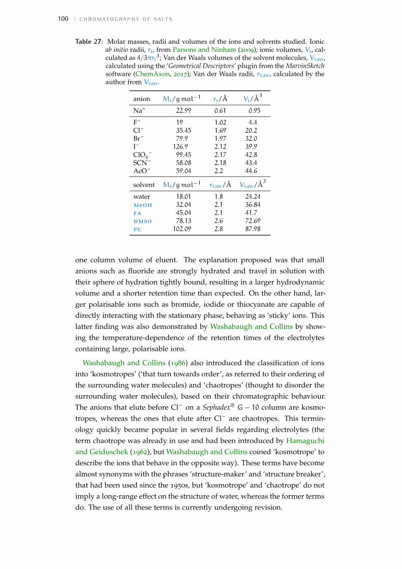
100 chromatography of salts
Table 27: Molar masses, radii and volumes of the ions and solvents studied. Ionicab initio radii, ri, from Parsons and Ninham (2009); ionic volumes, Vi, cal-culated as 4/3πri
3; Van der Waals volumes of the solvent molecules, VVdW,calculated using the ‘Geometrical Descriptors’ plugin from the MarvinSketchsoftware (ChemAxon, 2017); Van der Waals radii, rVdW, calculated by theauthor from VVdW.
anion Mi/gmol−1 ri/Å Vi/Å3
Na+ 22.99 0.61 0.95
F– 19 1.02 4.4Cl– 35.45 1.69 20.2Br– 79.9 1.97 32.0I– 126.9 2.12 39.9ClO4
– 99.45 2.17 42.8SCN– 58.08 2.18 43.4AcO– 59.04 2.2 44.6
solvent Mi/gmol−1 rVdW/Å VVdW/Å3
water 18.01 1.8 24.24meoh 32.04 2.1 36.84fa 45.04 2.1 41.7dmso 78.13 2.6 72.69pc 102.09 2.8 87.98
one column volume of eluent. The explanation proposed was that smallanions such as fluoride are strongly hydrated and travel in solution withtheir sphere of hydration tightly bound, resulting in a larger hydrodynamicvolume and a shorter retention time than expected. On the other hand, lar-ger polarisable ions such as bromide, iodide or thiocyanate are capable ofdirectly interacting with the stationary phase, behaving as ‘sticky’ ions. Thislatter finding was also demonstrated by Washabaugh and Collins by show-ing the temperature-dependence of the retention times of the electrolytescontaining large, polarisable ions.
Washabaugh and Collins (1986) also introduced the classification of ionsinto ‘kosmotropes’ (‘that turn towards order’, as referred to their ordering ofthe surrounding water molecules) and ‘chaotropes’ (thought to disorder thesurrounding water molecules), based on their chromatographic behaviour.The anions that elute before Cl– on a Sephadex® G− 10 column are kosmo-tropes, whereas the ones that elute after Cl– are chaotropes. This termin-ology quickly became popular in several fields regarding electrolytes (theterm chaotrope was already in use and had been introduced by Hamaguchiand Geiduschek (1962), but Washabaugh and Collins coined ‘kosmotrope’ todescribe the ions that behave in the opposite way). These terms have becomealmost synonyms with the phrases ‘structure-maker’ and ‘structure breaker’,that had been used since the 1950s, but ‘kosmotrope’ and ‘chaotrope’ do notimply a long-range effect on the structure of water, whereas the former termsdo. The use of all these terms is currently undergoing revision.

6.3 description of the technique 101
These experiments contributed to the formulation of the law of matchingwater affinities (lmwa) (Collins, 1997, 2004; Collins, Neilson et al., 2007)and also provided evidence for the importance of dispersion forces on thebehaviour of ions in water (Kunz, Belloni et al., 2004; Ninham, Duignan etal., 2011; Parsons, Boström, Lo Nostro et al., 2011; Salis and Ninham, 2014).
6.3 description of the techniqueSize-exclusion chromatography (sec) is a type of liquid column chromato-graphy that uses the stationary phase as a sieve in order to separate analytes ‘chromatography’
indicates a family oflaboratory techniquesemployed in theseparation of mixtures
according to their solvodynamic volume. Through calibration, the molecularweight of each separated fraction can be indirectly estimated.
sec can be employed for preparative or analytical purposes. It is popu-lar for the fractionation of proteins and for the characterisation of polymermixtures.
It is the only type of chromatography where no interaction is soughtbetween the analyte and the stationary phase. The column therefore actsmerely as a sieve. The separation or characterisation of a substance of a par-ticular solvodynamic radius (which includes the size of the molecule or ionand any tightly bound solvent), is therefore obtained on a purely entropicbasis. Separation is based on differences in the average path an analyte tra-verses inside the column. This is correlated to the size of the analyte withrespect to the porosity of the stationary phase. More accurately, the analytepartitions between the moving eluent phase outside the pore space, and thepools of stationary eluent inside the pores (Striegel et al., 2009). If the mo-lecule is sufficiently large that it is excluded from accessing the pores of thestationary phase, its path will be short and it will exit the column togetherwith the eluent front. Alternatively, if the analyte can access the pores, therewill be a fraction of its molecules inside the pores at any time, and thereforeits elution volume will be greater the smaller the analyte size. The longestpaths are available when the solute can access all the porosity. In practicalterms this is when the solute is as small as the molecules of solvent.
The eluted analyte is characterised by its retention factor Ksec (Striegel etal., 2009; Tayyab et al., 1991):
Ksec = (Vr − V0)/Vi [9]
where Vr is the retention volume of the analyte peak, V0 is the void volumeof the column (the volume of the interstitial mobile phase), and Vi is theinternal pore volume of the column (the stagnant volume of solvent trappedinside the stationary phase pores). A Ksec = 0 indicates that the analyteis completely excluded from accessing the stationary phase pores, whereas
102 chromatography of salts
Ksec = 1 indicates that the analyte accesses all volumes accessible to thesolvent. Molecules with intermediate sizes will display a retention factorbetween 0 and 1, proportional to their size. A Ksec > 1 is indicative of specificabsorption to the stationary phase packing and is a non-ideal condition thatviolates the assumption of exclusively entropic separation.
Experimentally, the void volume V0 is measured by running a sample thatis larger than the cut-off porosity of the stationary phase. A common choicefor determining V0 is Blue Dextran. This is what was used where possible.The internal pore volume Vi can be measured by subtracting V0 from theelution volume of a molecule of similar size to the eluent. As the detectionof such a molecule is often difficult (in the past radioactive labelling wasused), a molecule larger than the eluent but much smaller than the analyteis used, or the total geometric volume Vt of the column is used as an estimateof the internal volume. This is simply the volume of the cylinder with thesame height and radius of the stationary phase of the column. In this secondcase, Ksec is approximated as Kav (available) where:
Kav = (Vr − V0)/(Vt − V0) [10]
As this estimate does not account for the volume occupied by the packingmaterial and of the molecules of solvent tightly bound to the packing, thismethod results in an underestimation of the real retention factor of the ana-lyte.
Both Ksec and Kav are independent of the stationary phase height andare therefore useful in comparing different packings of the same stationaryphase. In addition, Ksec contains information about the physical distributionof the analyte in the column.
The calibration of the column can be performed by a series of solutesthat behave ‘ideally’, are of known molecular weight and are monodisperse.These can be proteins, peptides, polymers, olygomers based on the tech-nique being used and the molecular weights of interest. For established secprocedures, calibration kits are commercially available. In the present workI have attempted to calibrate the column but with no success.
The detection of the analyte can be performed by monitoring chemicalor physical properties of the eluate, depending on the properties of the ana-lytes and of the eluent; popular techniques include differential refractometry,spectroscopy (mostly uv-vis, but also Fourier-transform infrared spectro-scopy (ft-ir) and nmr), viscometry.

6.4 experiment details 103
6.4 experiment detailsThe chromatographic arrangement and experiment procedures used by Wa-shabaugh and Collins (1986) were followed where possible. Though, sub-stantial differences could not be avoided in our experiments, and are sum-marised in Section 6.4.6. The usage of non-aqueous solvents presents a num-ber of challenges including the measurement of the void volume and internalvolume. A detailed description of the methods we have used to determinethese volumes are included in Section 6.4.5.
6.4.1 Preparative tests
The same stationary phase as the one used by Washabaugh and Collins(1986) was used: Sephadex® G-10, epichlorohydrin-crosslinked dextran withan exclusion limit of 700Da. The gel is marketed for use in water, thereforeit was necessary to test its swelling and resistance to non-aqueous solvents.This was done by suspending one gram of Sephadex® in each of five vialsand adding an excess of anhydrous solvent or neat water. The swelling or-der after three days was as follows: pc � meoh < water < fa 6 dmso.Therefore the height of the column stationary phase was expected to vary inthe presence of different solvents. In pc very little swelling was observed.The swelling of the stationary phase is a critical parameter as it determinesthe column exclusion limit. With regards to stability of the Sephadex® sus-pensions, after 3 years of storage in the dark, no degradation was observedupon visual inspection.
As an automated system such as the GE Healthcare ÄKTA-Lab was notavailable, and it was anyway uncertain what effect non-aqueous solventswould have on several parts of the apparatus such as the gaskets, it waschosen to perform the chromatographic runs manually on an apparatus Iassembled.
6.4.2 Experiment apparatus and preparation
A 44 cm-long glass column was used, with an internal diameter of 1.63 cm(measured by caliper: 1.627 cm; measured by filling with a certain height ofwater and weighing the water: 1.630 cm), equipped with a 24/29 Quickfit®
cone and a Teflon® tap.
A schematic of the arrangement is in Fig. 18. The apparatus was mountedand run inside a fumehood.
A stainless steel connector and a Teflon® connector were made in-house inorder to connect the large bore glass outlets of the eluent reservoir and of
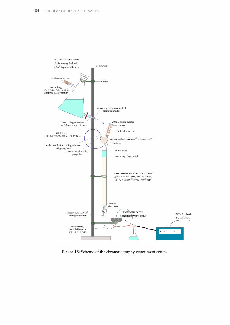
104 chromatography of salts
eluent reservoir1 l dispensing flask with
Teflon® tap and side arm support
molecular sieves
ptfe tubing,i.d. 8mm, o.d. 10mmwrapped with parafilm
ptfe tubing connector,i.d. 10mm, o.d. 12mm
fep tubing,i.d. 1.59mm, o.d. 3.175mm
male Luer lock to tubing adapter,polypropylene
stainless steel needle,gauge 20
clamp
custom-made stainless steeltubing connector
20ml plastic syringe
cotton
molecular sieves
rubber septum, aldrich® precision seal®
cable tie
eluent level
stationary phase height
chromatography columnglass, h = 440mm, i.d. 16.3mm,24/29 Quickfit® cone, Teflon® tap
silanisedglass wool
custom-made Teflon®
tubing connector
peek tubing,i.d. 0.7620mmo.d. 1.5875mm
flow-throughconductivity cell
conductivity
rs232 signalto laptop
Figure 18: Scheme of the chromatography experiment setup.

6.4 experiment details 105
the column to tubing. All the tubing was made of high chemical resistancepolymers: fep or ptfe, or polyether ether ketone (peek).
Detector
In order to detect the sample peak, we monitored the conductivity of theeluate and ran each sample separately. The detection by conductivity made itimpossible to use a NaCl solution as eluent, as in Washabaugh and Collins’swork (1986), because our tests showed that the conductivity signal to noiseratio of the sample peak was too small. Washabaugh and Collins (1986) hadused a NaCl solution as eluent in order to minimise the ion-exchange effectsof the hydroxyl groups on the Sephadex® surface.
Our trials in meoh show that the peak position is not substantially af-fected when using pure eluent in place of a salt solution. For the initial trials,the conductivity of the eluate was checked with a dip-in probe connected toa TPS smartCHEM-LAB multi-parameter laboratory analyser. The laboratoryconductivity sensor, also supplied by TPS, had a cell constant k = 1.0. Thissensor needs to be immersed in at least 15ml of sample in order to measureits conductivity. Once it was ascertained that the non-aqueous chromato-graphy experiment was feasible, it was evident that a resolution of 15mlin monitoring the eluate conductivity was too low. A custom-built flow-through conductivity cell was therefore made in-house. The design of thiscustom-made cell aimed at obtaining a detector with a small dead volumeto have a good resolution, with sufficient sensitivity, and that would be res-istant to the range of different solvents that we were going to use. This flow-through cell consists of a hollow peek cylinder, sealed at the two extremitiesby two threaded stainless steel electrodes. The design of the conductivity cellis reproduced in Fig. 92 of Appendix E. The inlet and outlet to the cell areperpendicular to the main cavity of the cylinder, so that the solution flowsparallel to the electrodes surface. The total volume of the chamber is about1ml. The cell is mounted with the electrodes in a horizontal position and theinlet tube at the bottom, so that the internal chamber completely fills withthe eluate without leaving air pockets. The electrodes send the signal to theTPS smartCHEM-LAB unit, which records the conductivity in auto-loggingmode, every 30 s. The conductivity readings from the TPS smartCHEM-LABunit are sent through an RS232 to USB 2.0 port adapter to a laptop, wherethey are processed by the Termite 3.3 RS232 terminal (Compu Phase, 2015).Despite this cell being of rudimental construction and despite the inferiorperformance of stainless steel with respect to platinised platinum (the ma-terial of choice for conductivity cell electrodes), it shows a linear response atlow conductivity as shown in Fig. 19. The sensitivity is about one fourth ofthe TPS dip-in probe in the linear region.

106 chromatography of salts
κ = 131132m2 + 13.1, r2 = 0.9996
κ = 135848m2 + 38.2, r2 = 0.9988
κ = 30033m2 + 8.8, r2 = 0.9975
κ = 28327m2 + 19.2, r2 = 0.9953
κ = 18526m2 + 22.6, r2 = 0.9824
κ = 45193m2 + 60.1, r2 = 0.9957
κ = 75420m2 + 14.7, r2 = 0.9985
κ = 9569m2 + 20.7, r2 = 0.9876
κ = 17925m2 + 4.2, r2 = 0.9975
κ = 17835m2 + 4.1, r2 = 0.9983
KCl in water NaCl in methanol
dip-inprobe
customprobe
0.00 0.01 0.02 0.03 0.04 0.05 0.00 0.01 0.02 0.03 0.04 0.05
0
2000
4000
6000
0
250
500
750
m/(molkg−1)
cond
ucti
vityκ/(µScm
−1)
Figure 19: Calibration curves for the custom made conductivity probe against theTPS probe. The shadings around the fitting lines represent a 95% confid-ence interval.
Column silanisation
The column was silanised before packing. Given its dimensions, it was notpossible to carry out the silanisation inside a desiccator. The column wasprepared for the silanisation procedure by washing it with a 10% NaOHsolution, thoroughly rinsing it with Type I ultrapure water, and drying inan oven at 85 ◦C overnight (the glass wool, the tap and a stopper for thetop Quickfit® cone were washed and dried in the oven as well). The fol-lowing morning, the column was taken out of the oven and assembled andstoppered swiftly. A quick procedure for silanising was carried out as fol-lows in a fumehood: a few drops of chlorotrimethylsilane (aldrich®) wereintroduced with a 1ml plastic syringe while the column was still warm andthe stopper quickly put back. The chlorotrimethylsilane quickly evaporatedto react with the silanol groups of the glass.
The column was kept stoppered and sealed with Parafilm M® until pack-ing.
Column packing
The packing of the column was performed in meoh as it was the first elu-ent I intended to test. Also, as meoh is less viscous than fa and dmso,I expected packing to be faster in this solvent as the flow rate would behigher. All of the operations were performed rapidly in order to let as littlemoisture as possible into the column. None of the solvents and solutionsused were filtered or degassed. All of the operations were performed in afumehood. The packing of the column was performed with the conductivityprobe already connected to the column. This was done especially to avoiddisturbing the packing as the insertion of the ptfe column outlet-to-tubingadapter required some force.

6.4 experiment details 107
The Sephadex® G-10 (≈ 53 g) was dried in an oven at 85 ◦C in a 250mlconical flask for 8h, the flask was then put in a desiccator to cool. An excessof dry meoh (≈ 150ml was subsequently added to the Sephadex®, the flaskwas sealed with aluminium foil and Parafilm M®, and left to swell overnightin a desiccator. As the column did not have a frit, a small amount of silan-ised glass wool was placed in the bottom throat of the column to prevent theSephadex® from going through the tap. The glass wool was tapped gently,trying to avoid compacting it too much, with a long glass rod to form a sur-face as even and horizontal as possible. Part of the supernatant meoh wasdiscarded from the Sephadex® suspension in order to obtain a thick slurry(≈ 75% settled Sephadex®), which was kept in suspension by delicately swirl-ing the flask. The column was filled with approximately 8 cm of neat dryeluent, the glass wool was tapped delicately with a long glass rod to elimin-ate the trapped air bubbles; the tap was then opened and the slurry poureddown a glass rod slowly in one motion. The glass rod was used to directthe slurry flow towards the inner wall of the column and prevent splashingand bubble incorporation in the slurry. As soon as the slurry pouring wasfinished, a cone 24 drying tube filled with molecular sieves was applied atthe top, to avoid the entrance of moisture, whilst allowing air through inorder to let the eluent flow. The tap was kept open and anhydrous meohadded at the top of the column (by removing and then replacing the dryingtube) to pack the stationary phase. More than one column volume (≈ 50ml)of solvent was eluted before closing the tap. When the tap was closed, thedrying tube on top was substituted with a stopper and sealed externallywith Parafilm M®. Parafilm M® was also applied around the closed columntap.
6.4.3 Experiment procedure
The day after packing in meoh, the height of the stationary phase was meas-ured, amounting to 32.3 cm. For the first sample run, an Aldrich PrecisionSeal® rubber septum (low in solvent extractables) for 24/40 joints was puton the top cone and the sleeve was bent over and secured with a cable tie.The rubber septum was always kept in place until the end of all of the ex-perimental runs in all of the eluents. It was replaced with a new one whenthe number of punctures was compromising the seal. The septum was punc-tured with the needle (25G) of a 20ml plastic syringe, from which the plun-ger had been removed and that had been filled with molecular sieves (keptin place by cotton wool at the end of the syringe), in order to equalize thecolumn to atmospheric pressure. Another needle (20G) was used to connectthe reservoir tubing and feed the eluent to the column.
108 chromatography of salts
At the end of each day, the two needles would be removed and capped,and the rubber septum covered with Parafilm M® as an additional protectionfrom moisture.
The eluent reservoir was refilled, when needed, with fresh anhydrous sol-vent from the storage bottle. Cannulation with dry nitrogen from the sol-vent storage bottle was tested in order to fill the eluent reservoir and keepthe eluent as anhydrous as possible, but as the cannulation procedure isextremely time-consuming for large volumes of solvent, it was decided toinstead transfer the solvent classically by using an oven-dried 250ml beakeras a transferring vessel. All of the operations were performed rapidly in afumehood.
The eluent reservoir was washed and dried periodically, especially whenchanging eluent in the column. The reservoir was sealed with Parafilm M®
at the end of each day to avoid the entrance of moisture and preserve themolecular sieves. Also the column rubber septum and tap were wrappedin aluminium foil and Parafilm M® overnight. The ptfe adapter for theconductivity cell tubing at the outlet of the column was never disconnected.
The concentration of each electrolyte sample was 5× 10⁻²molkg−1.
Sample loading
In order to load the sample, the eluent level in the column was lowereduntil it reached the top of the stationary phase. The column tap was thenclosed and the rubber septum was punctured with a 1ml Hamilton® syringemounting a 25G needle, which had just been rinsed with 0.5ml of sample,and filled with fresh sample. The syringe was emptied very slowly while itsneedle tip was kept close to the column wall so that the falling sample dropswould not disturb the column packing. The tap was opened immediately af-terwards, the Hamilton® syringe extracted from the rubber septum, and thesample was left to absorb on the stationary phase. As soon as the samplewas completely loaded, the eluent supply was restored by opening the reser-voir tap, and the eluent level above the stationary phase was restored toa marked level as quickly as possible, but still while being very careful toavoid disturbance of the column bed at the beginning of the addition. Atthe same time that the eluent supply was reopened, the conductivity-metreauto-logging was started, in order to record the conductivity of the eluate asa function of time.
Elution
In order to keep the column flow quite constant, the solvent reservoir tapwas adjusted so that there would always be a certain height of eluent abovethe stationary phase. This height was approximately 6 cm.
6.4 experiment details 109
During elution, the flow rate was monitored by measuring the time re-quired to fill a 5ml measuring cylinder with eluate (the cylinder was put inplace of the waste container, after the conductivity probe). For best accur-acy, during the anhydrous runs, the flow rate was measured continuouslyby alternating two measuring cylinders, that were dried after each use.
The conductivity was recorded on a laptop connected as described in Sec-tion 6.4.2. One conductivity reading was registered every 30 s, which corres-ponded to different amounts of eluted volume depending on the flow rate ofthe column. The flow rate-dependence on the solvent is shown in Table 28.The conductivity was manually plotted in real time in order to monitor theexperiment.
When the light sensitive NaI and NaSCN where eluted, the column waswrapped in aluminium foil.
Sometimes bubbles would form or be trapped in the conductivity sensorchamber due to the inlet tubing leaking, causing oscillations in the conduct-ivity reading. Because of the material and the narrow bore of the outlettubing, they would not leave the measuring chamber spontaneously andthey had to be manually removed by pulling out the outlet tubing from thechamber and letting the air bubble exit.
Usually only one sample was chromatographed per day due to the slowflow rate of the column.
6.4.4 Eluent change
The same Sephadex® column packing was used for all eluents, which werechanged in sequence in the order meoh − fa − dmso − pc (− dmsobecause pc and water only have a narrow miscibility range) − H2O. Allelectrolytes that were soluble in that eluent were run on the column, andthen the solvent was changed. The change from one eluent to the next wasperformed by passing eluent mixtures at increasing volume content of thenew eluent. A typical solvent change would be made in four steps, and atleast one column volume (40ml) of mixture was eluted in each step: firsta 3 : 1 (old eluent : new eluent) mixture, followed by a 1 : 1 (old : new)solution, then a 1 : 3 (old : new) mix, and finally at least one column volumeof neat new eluent. The gradual solvent change was done to minimise stresson the stationary phase due to swelling or shrinking in the new solvent.
Sephadex® swells differently in the solvents, and the height of the packingand the other column parameters are listed in Table 28. The column heightwas stable during the experiments in each solvent.
flow rate dependence on eluent type As the flow was gravity-driven, it is also interesting to comment on the flow rate in the different
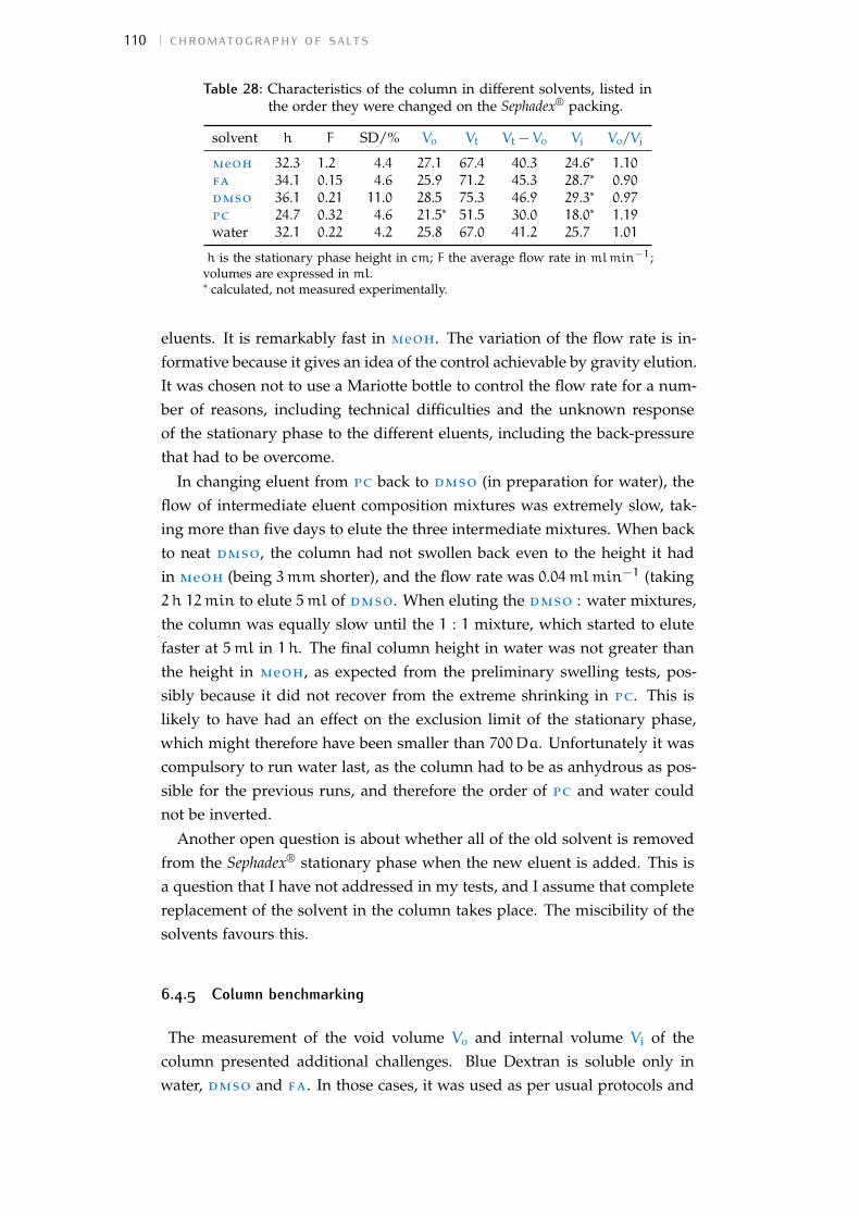
110 chromatography of salts
Table 28: Characteristics of the column in different solvents, listed inthe order they were changed on the Sephadex® packing.
solvent h F SD/% V0 Vt Vt − V0 Vi V0/Vi
meoh 32.3 1.2 4.4 27.1 67.4 40.3 24.6* 1.10fa 34.1 0.15 4.6 25.9 71.2 45.3 28.7* 0.90dmso 36.1 0.21 11.0 28.5 75.3 46.9 29.3* 0.97pc 24.7 0.32 4.6 21.5* 51.5 30.0 18.0* 1.19water 32.1 0.22 4.2 25.8 67.0 41.2 25.7 1.01
h is the stationary phase height in cm; F the average flow rate in mlmin−1;volumes are expressed in ml.* calculated, not measured experimentally.
eluents. It is remarkably fast in meoh. The variation of the flow rate is in-formative because it gives an idea of the control achievable by gravity elution.It was chosen not to use a Mariotte bottle to control the flow rate for a num-ber of reasons, including technical difficulties and the unknown responseof the stationary phase to the different eluents, including the back-pressurethat had to be overcome.
In changing eluent from pc back to dmso (in preparation for water), theflow of intermediate eluent composition mixtures was extremely slow, tak-ing more than five days to elute the three intermediate mixtures. When backto neat dmso, the column had not swollen back even to the height it hadin meoh (being 3mm shorter), and the flow rate was 0.04mlmin−1 (taking2h 12min to elute 5ml of dmso. When eluting the dmso : water mixtures,the column was equally slow until the 1 : 1 mixture, which started to elutefaster at 5ml in 1h. The final column height in water was not greater thanthe height in meoh, as expected from the preliminary swelling tests, pos-sibly because it did not recover from the extreme shrinking in pc. This islikely to have had an effect on the exclusion limit of the stationary phase,which might therefore have been smaller than 700Da. Unfortunately it wascompulsory to run water last, as the column had to be as anhydrous as pos-sible for the previous runs, and therefore the order of pc and water couldnot be inverted.
Another open question is about whether all of the old solvent is removedfrom the Sephadex® stationary phase when the new eluent is added. This isa question that I have not addressed in my tests, and I assume that completereplacement of the solvent in the column takes place. The miscibility of thesolvents favours this.
6.4.5 Column benchmarking
The measurement of the void volume V0 and internal volume Vi of thecolumn presented additional challenges. Blue Dextran is soluble only inwater, dmso and fa. In those cases, it was used as per usual protocols and

6.4 experiment details 111
detected both visually and by uv-vis spectroscopy on collected fractions ofthe eluate (fraction volume ≈ 1ml), by monitoring the peak at 630nm. Inthe case of meoh, instead, a sample of PVP-360 (polyvinylpirrolidone ofaverage molecular weight = 360 000Da), at concentration wpvp= 0.0028 wasused and detected by uv absorbance at 210nm. In pc, despite PVP-360being soluble, it was not possible to detect it and only an estimate of V0 wasmade based on the elution profiles of the electrolytes peaks. It is possiblethat this is because pc itself absorbs at 210nm, or because of residual iodidein the column that was not possible to remove (NaI behaves as highly stickyin pc).
Several molecules were tested in a trial column packing in meoh in orderto calibrate the column: DiI, 1, 1 ′-dioctadecyl-3, 3, 3 ′, 3 ′-tetramethyl-indo-carbocyanine perchlorate, (Mi = 933.87 gmol−1), methylene blue (Mi =
319.85 gmol−1) and crystal violet (Mi = 407.98 gmol−1). All of these mo-lecules showed non-ideal behaviour and formed large bands with very longelution times. Also glucose (Mi = 180.1559 gmol−1) was trialled as a mo-lecule for calibration, and I attempted its detection by differential refractivityindex measurement (by measuring distinct fractions in a non-flow throughinstrument), but it was not possible to detect it accurately. This is possiblydue to the low concentration of the glucose solutions, given its low solubilityin meoh.
In water, D2O (sample size 1ml) was successfully used for determining Vi
and detected by measuring the T2 nmr relaxation time of the eluate fractionswith a XIGO Nanotools Acorn Area instrument. This technique could havealso been used for the other eluents, by running their corresponding deu-terated solvent, but this approach was only discovered after the last eluentchange to water, and it was not feasible to change back to the non-aqueoussolvents (mainly because of the possibility of water contamination). An es-timate of the internal volume for the column in the other solvents was there-fore calculated as a proportion of their geometric volume Vt, by using theinternal volume to geometric volume ratio Vi/Vt found for water. This isof course an estimate of the internal volume that is an approximation, but Ithink that it is more informative than using the geometric volume. In fact,in the column (Vt − V0) is about 60% larger than Vi, therefore the differencebetween the two cannot be ignored when one wants to interpret the parti-tion coefficient in terms of the distribution of the sample between the voidvolume and the internal pore volume. It follows that Kav is not an accept-able estimate of Ksec when one is looking for information about the sampledistribution. See Table 28 for the values in the various solvents.
Another observation that must be made about the values in Table 28 isabout the void volume V0 to total geometric volume Vt ratio: the first is usu-ally reported to be around 30% − 35% of the swollen stationary phase (Tay-
112 chromatography of salts
yab et al., 1991), but in this case it amounts to 40%. This could be an intrinsicproperty of Sephadex® G-10, as it is highly crosslinked.
In addition, the ratio V0/Vi expresses the porosity of the stationary phase,and it is the smallest in pc, followed by meoh, then water, fa and dmso.The size of the substances that are excluded from the internal porosity istherefore affected by this parameter, with the Sephadex® swollen in pc exclud-ing smaller molecules from its internal pores than the Sephadex® in dmso,which has a larger exclusion limit than water.
6.4.6 Differences from Washabaugh and Collins’s experiment
This section summarises the substantial differences between our experimentprocedure and the one detailed by Washabaugh and Collins (1986).
• The stationary phase height in this work was approximately 30 cm
rather than 85.5 cm, although Washabaugh and Collins made tests ona shorter column and obtained the same results.
• The column temperature was controlled by Washabaugh and Collinsat 30 ◦C through a circulating water bath. In my experiments this wasnot controlled, rather the experiments were conducted in an air condi-tioned room at approximately 22 ◦C.
• I did not filter or degas the eluent and samples.
• The detection of the sample peak was performed by conductivity, thusa neat eluent was used rather than a 0.1mol dm−3 solution of NaCl.
• The flow rate was gravity driven rather than set by using a Mari-otte bottle, and this resulted in flow rates that were more variablefrom solvent to solvent. Washabaugh and Collins set the flow rateat 0.5mlmin−1.
• The concentration of the sample was 5× 10⁻²molkg−1 rather than0.1mol dm−3 because of the lower solubility of salts in the non-aque-ous solvents.
• The internal volume of the column was measured by running a D2Osample rather than tritiated water. It was also only determined inwater.
6.5 results and detailed discussion 113
6.5 results and detailed discussionThis section contains an in-depth discussion of the chromatograms. Theresults in regards to the solvent effects on sie and the overarching trendsare discussed in the ensuing section, Section 6.6.
Chromatograms were measured for a range of electrolytes in water, meoh,fa, dmso and pc in order to investigate the influence of the solvent onthe ion specificity of elution. More than 100 chromatography runs wereperformed in total.
For all of the chromatograms, the baseline conductivity of the pure sol-vent has been subtracted and the values of the conductivity rescaled relativeto the maximum conductivity being set to 1. This maximum conductivityequals 467µS cm−1 in water, 22.44µS cm−1 in meoh, 103.5µS cm−1 in fa,53.1µS cm−1 in dmso and 4.91µS cm−1 in pc. Although these values havebeen measured with the custom-made conductivity cell we built and cannottherefore be regarded as accurate absolute values, they do give an idea of thedifferent conductivities in the various solvents. Also the average neat solventconductivity (baseline) changed: 3µS cm−1 in water, 0.2µS cm−1 in meoh,40µS cm−1 in fa, 0.05µS cm−1 in dmso and 0.02µS cm−1 in pc. Again,these values are approximate estimates of the real values, but it is noticeablethat fa has a much higher conductivity. This is due to the fact that in thepresence even of low quantities of moisture, fa hydrolyses to ammoniumformate. Very dry fa had been purchased, but the presence of traces ofmoisture in the chromatography path cannot be completely excluded.
Based on the sizes of the ions (Table 27), the ordering of elution expectedin ideal conditions is CH3COO− − SCN− − ClO4
− − I− − Br− − Cl− − F−,although the shapes of the polyatomic ions thiocyanate, perchlorate andacetate are expected to have an influence on their solvodynamic radius andtherefore may influence their positioning.
Water is the only solvent in which I have measured the internal volume, Vi,accurately in addition to the void volume, V0. For all of the non-aqueous sol-vents, only the geometric volume of the packing has been measured and theinternal volume has been estimated by using the ratio of internal volume togeometric volume found for water — noting that the swelling of the columnis solvent dependent (see Section 6.4.5). Such an estimate of the internalvolume is not accurate due to the different levels of swelling and differentmolar volumes of the different solvents. However, I think it is still a betterestimate than the geometric volume, particularly for interpreting the elutionof electrolytes. Therefore, I have used the estimate of the internal volume forthe calculation of Ksec. Regardless, my primary interest is in the ion-specifictrends in each solvent and these are not impacted by the calculation of Ksec.The (measured) geometric volume and void volume, and the calculated in-
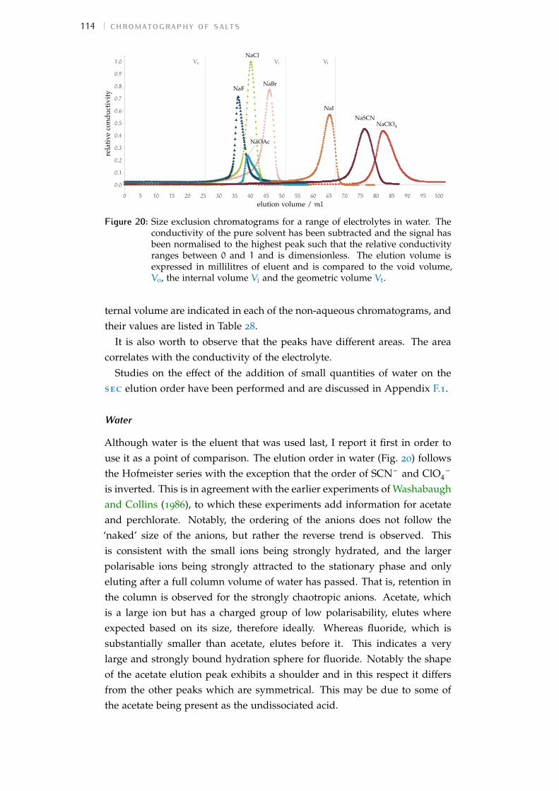
114 chromatography of salts
V0 VtVi
NaBr
NaCl
NaClO4
NaF
NaI
NaOAc
NaSCN
0.0
0.1
0.2
0.3
0.4
0.5
0.6
0.7
0.8
0.9
1.0
0 5 10 15 20 25 30 35 40 45 50 55 60 65 70 75 80 85 90 95 100
elution volume / ml
rela
tive
cond
ucti
vity
Figure 20: Size exclusion chromatograms for a range of electrolytes in water. Theconductivity of the pure solvent has been subtracted and the signal hasbeen normalised to the highest peak such that the relative conductivityranges between 0 and 1 and is dimensionless. The elution volume isexpressed in millilitres of eluent and is compared to the void volume,V0, the internal volume Vi and the geometric volume Vt.
ternal volume are indicated in each of the non-aqueous chromatograms, andtheir values are listed in Table 28.
It is also worth to observe that the peaks have different areas. The areacorrelates with the conductivity of the electrolyte.
Studies on the effect of the addition of small quantities of water on thesec elution order have been performed and are discussed in Appendix F.1.
Water
Although water is the eluent that was used last, I report it first in order touse it as a point of comparison. The elution order in water (Fig. 20) followsthe Hofmeister series with the exception that the order of SCN– and ClO4
–
is inverted. This is in agreement with the earlier experiments of Washabaughand Collins (1986), to which these experiments add information for acetateand perchlorate. Notably, the ordering of the anions does not follow the‘naked’ size of the anions, but rather the reverse trend is observed. Thisis consistent with the small ions being strongly hydrated, and the largerpolarisable ions being strongly attracted to the stationary phase and onlyeluting after a full column volume of water has passed. That is, retention inthe column is observed for the strongly chaotropic anions. Acetate, whichis a large ion but has a charged group of low polarisability, elutes whereexpected based on its size, therefore ideally. Whereas fluoride, which issubstantially smaller than acetate, elutes before it. This indicates a verylarge and strongly bound hydration sphere for fluoride. Notably the shapeof the acetate elution peak exhibits a shoulder and in this respect it differsfrom the other peaks which are symmetrical. This may be due to some ofthe acetate being present as the undissociated acid.

6.5 results and detailed discussion 115
Although we observe the same elution order as Washabaugh and Collins(1986), some discrepancies in the experiment results are present: in their case,bromide was eluting after the tritiated water (internal volume) peak with aKav of 1.2, thus supporting the hypothesis that Cl– behaves ideally and is thewatershed ‘neutral’ ion between chaotropes and kosmotropes. This was alsosupported by the calibration performed by Washabaugh and Collins with theaminoacid glycine and its polymers up to hexaglycine (Mi = 75 gmol−1 to360 gmol−1), although as both the aminoacid and the oligopeptides exist insolution as zwitterions, doubts about their aptness as calibrating referencesarise, given that they are ionic themselves. In our case, though, also bromideelutes within the first column volume, with a Kav of 0.8. This might be an in-dication of the fact that the different experiment conditions are considerablyinfluencing the observed retention factors.
Also the NaI peak shape is notably different, with it being slightly frontingin my experiments, versus noticeably tailing in Washabaugh and Collins’s.Fronting and tailing peaks are asymmetrical peaks, that do not have the idealGaussian peak profile, and where the skewed part either precedes (front-ing) or trails behind (tailing) the peak. Fronting is usually associated withcolumn overloading or a flawed packing of the stationary phase, whereastailing indicates specific interaction with the stationary phase (the analyteis retained anomalously), or extra-column effects. However, in sec, thefronting, tailing and splitting of peaks can also be induced by reversibleassociation of the analyte in solution, such as in the formation of dimers.Theoretical studies on protein association in sec predict that, when theassociation and dissociation rates are comparable to the convection rate, amerged, broad peak forms, with either fronting when dimers dominate ortailing when monomers dominate (Yu et al., 2006). In fronting, as the dimersmove ahead of the monomers, they dissociate into monomers themselves,which migrate more slowly, thus producing a self-sharpening advancingwave. When both the association and dissociation kinetics are slow, splitpeaks form. For ions in solution, the associated species have to be identified.It is possible that they are contact or solvent-shared ion pairs in solution (Yuet al., 2006).
The behaviour and series we observe in water is of reference to the beha-viours observed in the non-aqueous solvents, which are discussed below.
Methanol
The elution order in meoh (Fig. 21) follows precisely the same order as wa-ter. The overall elution volumes are much greater and all of the electrolytesrequired an elution volume greater than the internal volume, suggesting thatall of the ions except acetate and fluoride interact with the column i.e. are‘sticky’, but the degree with which they interact with the column remains
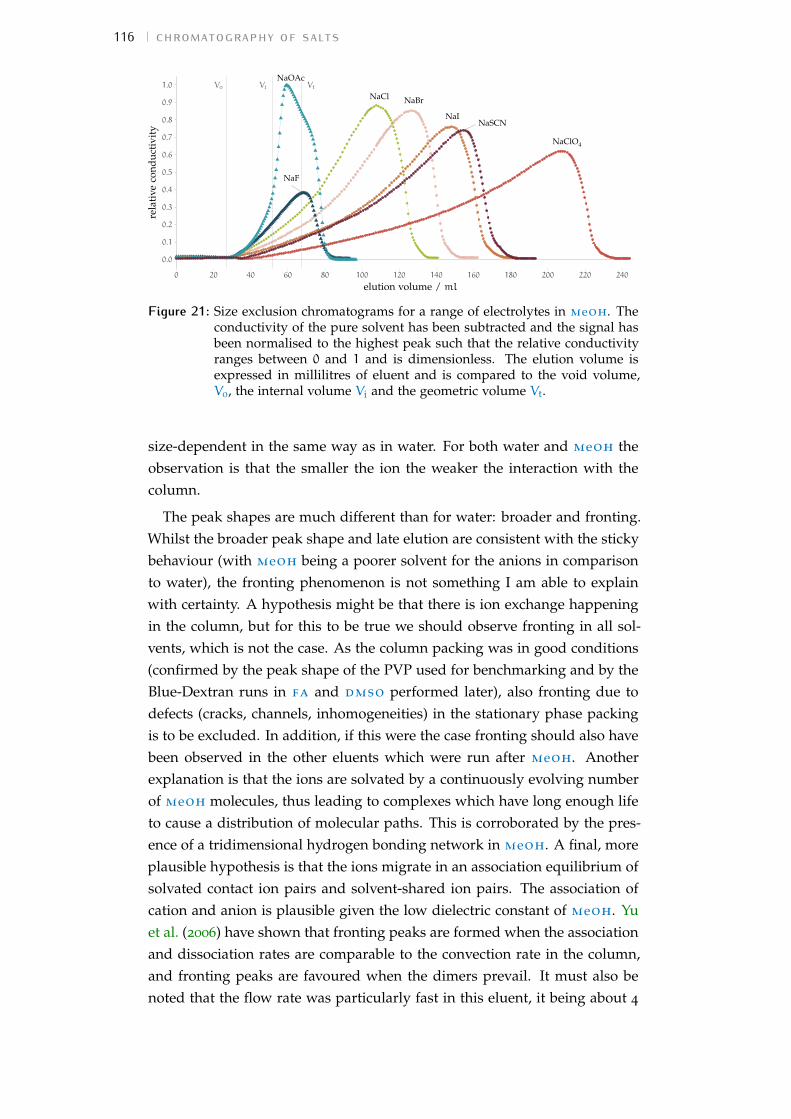
116 chromatography of salts
V0 VtVi
NaBrNaCl
NaClO4
NaF
NaI
NaOAc
NaSCN
0.0
0.1
0.2
0.3
0.4
0.5
0.6
0.7
0.8
0.9
1.0
0 20 40 60 80 100 120 140 160 180 200 220 240
elution volume / ml
rela
tive
cond
ucti
vity
Figure 21: Size exclusion chromatograms for a range of electrolytes in meoh. Theconductivity of the pure solvent has been subtracted and the signal hasbeen normalised to the highest peak such that the relative conductivityranges between 0 and 1 and is dimensionless. The elution volume isexpressed in millilitres of eluent and is compared to the void volume,V0, the internal volume Vi and the geometric volume Vt.
size-dependent in the same way as in water. For both water and meoh theobservation is that the smaller the ion the weaker the interaction with thecolumn.
The peak shapes are much different than for water: broader and fronting.Whilst the broader peak shape and late elution are consistent with the stickybehaviour (with meoh being a poorer solvent for the anions in comparisonto water), the fronting phenomenon is not something I am able to explainwith certainty. A hypothesis might be that there is ion exchange happeningin the column, but for this to be true we should observe fronting in all sol-vents, which is not the case. As the column packing was in good conditions(confirmed by the peak shape of the PVP used for benchmarking and by theBlue-Dextran runs in fa and dmso performed later), also fronting due todefects (cracks, channels, inhomogeneities) in the stationary phase packingis to be excluded. In addition, if this were the case fronting should also havebeen observed in the other eluents which were run after meoh. Anotherexplanation is that the ions are solvated by a continuously evolving numberof meoh molecules, thus leading to complexes which have long enough lifeto cause a distribution of molecular paths. This is corroborated by the pres-ence of a tridimensional hydrogen bonding network in meoh. A final, moreplausible hypothesis is that the ions migrate in an association equilibrium ofsolvated contact ion pairs and solvent-shared ion pairs. The association ofcation and anion is plausible given the low dielectric constant of meoh. Yuet al. (2006) have shown that fronting peaks are formed when the associationand dissociation rates are comparable to the convection rate in the column,and fronting peaks are favoured when the dimers prevail. It must also benoted that the flow rate was particularly fast in this eluent, it being about 4
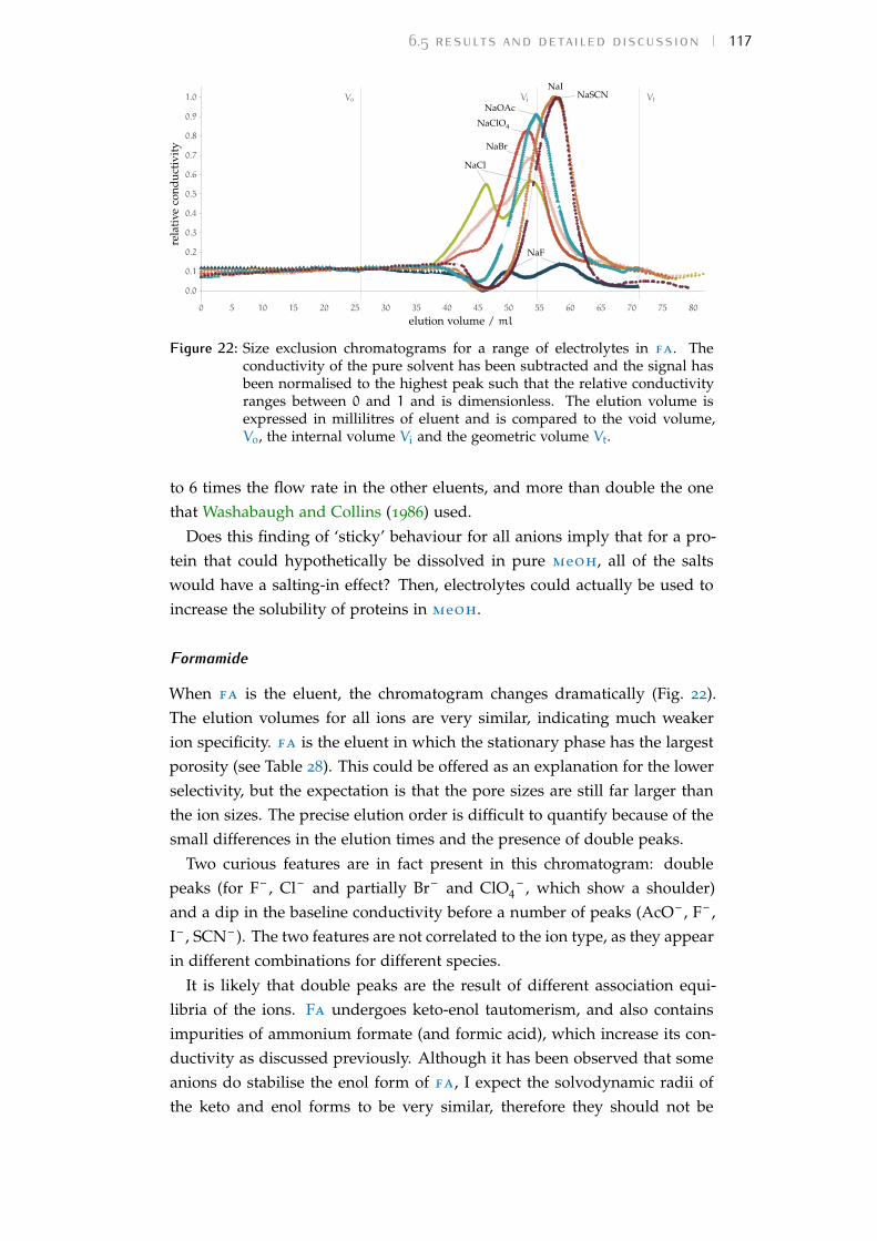
6.5 results and detailed discussion 117
V0 VtVi
NaBr
NaCl
NaClO4
NaF
NaI
NaOAcNaSCN
0.0
0.1
0.2
0.3
0.4
0.5
0.6
0.7
0.8
0.9
1.0
0 5 10 15 20 25 30 35 40 45 50 55 60 65 70 75 80
elution volume / ml
rela
tive
cond
ucti
vity
Figure 22: Size exclusion chromatograms for a range of electrolytes in fa. Theconductivity of the pure solvent has been subtracted and the signal hasbeen normalised to the highest peak such that the relative conductivityranges between 0 and 1 and is dimensionless. The elution volume isexpressed in millilitres of eluent and is compared to the void volume,V0, the internal volume Vi and the geometric volume Vt.
to 6 times the flow rate in the other eluents, and more than double the onethat Washabaugh and Collins (1986) used.
Does this finding of ‘sticky’ behaviour for all anions imply that for a pro-tein that could hypothetically be dissolved in pure meoh, all of the saltswould have a salting-in effect? Then, electrolytes could actually be used toincrease the solubility of proteins in meoh.
Formamide
When fa is the eluent, the chromatogram changes dramatically (Fig. 22).The elution volumes for all ions are very similar, indicating much weakerion specificity. fa is the eluent in which the stationary phase has the largestporosity (see Table 28). This could be offered as an explanation for the lowerselectivity, but the expectation is that the pore sizes are still far larger thanthe ion sizes. The precise elution order is difficult to quantify because of thesmall differences in the elution times and the presence of double peaks.
Two curious features are in fact present in this chromatogram: doublepeaks (for F– , Cl– and partially Br– and ClO4
– , which show a shoulder)and a dip in the baseline conductivity before a number of peaks (AcO– , F– ,I– , SCN– ). The two features are not correlated to the ion type, as they appearin different combinations for different species.
It is likely that double peaks are the result of different association equi-libria of the ions. Fa undergoes keto-enol tautomerism, and also containsimpurities of ammonium formate (and formic acid), which increase its con-ductivity as discussed previously. Although it has been observed that someanions do stabilise the enol form of fa, I expect the solvodynamic radii ofthe keto and enol forms to be very similar, therefore they should not be
118 chromatography of salts
able to give a split peak. A different plausible species in solution mightoriginate from the association of the anion with the ammonium of the freeammonium formate, and this would be expected especially for softer anions.In fact, based on the lmwa, the softer anions might have favourable interac-tions also with ammonium, but this does not explain the presence of doublepeaks for chloride and bromide which are kosmotropes. In addition, whilefor the chaotropes the second peak is a shoulder, for the kosmotropes thetwin peaks have almost identical areas. It is not easy to estimate whetherthere is enough ammonium formate in solution to create a second peak asbig as the one from NaX, although the lmc of NH4
+ is higher than that ofNa+ (Table 6 in Chapter 2), therefore a smaller concentration of the formergives a larger peak signal. This is corroborated by the fact that the peak con-ductivity is about double the conductivity of the baseline, therefore thereis not a huge difference. It is not possible, though, to account for the con-centrations of each ion in solution as their conductivities are different. It islikely therefore that there are two distinct causes for the formation of doublepeaks, one which leads to double peaks for kosmotropes and the other forchaotropes. further analysis would be required to determine the chemicalcomposition of the two different peaks. If the chemical species are the same,then the two peaks are likely the result of different associated entities insolution, and the structure of the solution should be investigated. Althoughthese should have very long lifetimes. This is also suggested by researchthat shows that peak splitting is favoured at a high linear velocity (not ourcase), for a short column length (which is the case for this experiment), orfor relatively slow association and dissociation rates (Yu et al., 2006).
The dip in the baseline conductivity is another puzzle, for which I donot have an explanation. It happens both for double peaks (F– ) and forsingle peaks (I– and SCN– ). As already explained, fa has a higher baselineconductivity due to the presence of ammonium formate, the product of thehydrolysis of fa in the presence of trace quantity of water. The dip indic-ates that the concentration of ammonium formate is depleted right beforethe peak passes. It corresponds to a difference in conductivity of about5µS cm−1 (this quantity is measured with the custom-made conductivityprobe, therefore it is not a good estimate of the true value, and is likelysmaller by about a fourth) from a baseline that averages a 40µS cm−1 con-ductivity. If the HCOONH4 and NaX actually undergo a double exchangeof ions to some extent, then the conductivity of HCOONa is lower thanHCOONH4, and could therefore explain the dip in the baseline. But again,while the close association in solution of the ammonium with the chaotropicions I– and SCN– is expected, it is not as justified with acetate and fluoride,for which a dip in the baseline before the peak is observed as well.

6.5 results and detailed discussion 119
V0 VtVi
NaBr
NaCl
NaClO4
NaI
NaSCN
0.0
0.1
0.2
0.3
0.4
0.5
0.6
0.7
0.8
0.9
1.0
0 10 20 30 40 50 60 70 80 90 100 110 120 130
elution volume / ml
rela
tive
cond
ucti
vity
Figure 23: Size exclusion chromatograms for a range of electrolytes in dmso. Theconductivity of the pure solvent has been subtracted and the signal hasbeen normalised to the highest peak such that the relative conductivityranges between 0 and 1 and is dimensionless. The elution volume isexpressed in millilitres of eluent and is compared to the void volume,V0, the internal volume Vi and the geometric volume Vt.
Independently of the presence of these two unique chromatogram fea-tures, the overall behaviour in fa indicates that the solvation of kosmotropicand chaotropic anions in is much more similar in this solvent than in theother solvents investigated, and that also there is little or no interaction ofthe ions with the Sephadex® surface. The latter suggests that all ions arestrongly solvated, which is in agreement with the high dielectric constantand dipole moment of this solvent (Table 2 Chapter 1).
Dimethyl sulfoxide
The chromatogram for dmso (Fig. 23) shows the reversal of the elution pat-tern observed in protic solvents.
As such, the order observed is that expected based on the size of the anionalone. Whilst the order suggests that size is controlling the elution, longelution times for chloride and bromide indicate that they are interactingstrongly with the stationary phase. These sticky ions are now kosmotropicanions in contrast to water and meoh where they presented as sticky. In thiscase the smaller less polarisable ions have a greater affinity for the stationaryphase.
We are observing for the first time a reversal of the Hofmeister series dueto solvent effects (reversal has already been observed to happen in relation tosurface charge, concentration and pH, see Section 2.3).
All of the peak shapes indicate fronting, as was the case in meoh, butin this case the peak is more skewed for bromide and chloride, which isthe opposite of what happens in meoh. This suggests that dmso is alsoa quite poor solvent for practically all of the anions, that tend to exhibitassociation. Chloride and bromide, in addition, have more have favourable

120 chromatography of salts
V0 VtVi
NaClO4
NaI
NaSCN
0.0
0.1
0.2
0.3
0.4
0.5
0.6
0.7
0.8
0.9
1.0
0 5 10 15 20 25 30 35 40 45 50 55 60 65 70 75 80 85 90 95 100
elution volume / ml
rela
tive
cond
ucti
vity
Figure 24: Size exclusion chromatograms for a range of electrolytes in pc. Theconductivity of the pure solvent has been subtracted and the signal hasbeen normalised to the highest peak such that the relative conductivityranges between 0 and 1 and is dimensionless. The elution volume isexpressed in millilitres of eluent and is compared to the void volume,V0, the internal volume Vi and the geometric volume Vt.
interactions with the stationary phase and behave as sticky ions. This is alsoin agreement with the fact that aprotic solvent are less good solvents foranions, as indicated by their donor number. Interestingly though, in dmsosome ions are eluting within one column volume, which does not happen inmeoh. Both the dipole moment and dielectric constant of dmso are higher,so this is probably why it is more successful in solvating the anions overall.
Propylene carbonate
The range of electrolytes that could be studied in pc is limited (Fig. 24).The available data suggests similar behaviour to that observed in dmso.However, in this case, iodide behaves as strongly sticky. Its interaction withthe column was so strong that it altered the baseline for a number of runsafterwards. Although NaBr was not run in the anhydrous final runs, a testwith a saturated sample during the trial runs (Fig. 94 Chapter 5) shows thatit behaves as even stickier than NaI, thus confirming the reverse trend ofanions for dmso.
6.6 summaryI have successfully performed sec of sodium electrolytes in four non-aque-
ous solvents. Sec sheds light on the ion-solvent and ion-surface interactionin solution.
The elution behaviour for the various electrolytes is summarised in Fig. 25.Here the value of Ksec is shown for the various electrolytes (ordered from topto bottom as the Hofmeister series i.e. the fundamental series for anions) in
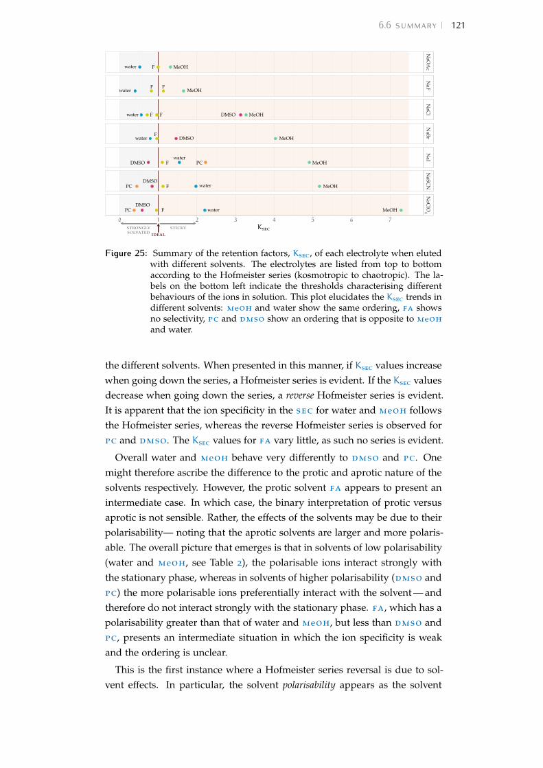
6.6 summary 121
F MeOHwater
F FMeOHwater
DMSOF F MeOHwater
DMSOF
MeOHwater
DMSO F MeOHPCwater
DMSOF MeOHPC water
idealstronglysolvated
sticky
DMSOF MeOHPC water
NaO
Ac
NaF
NaC
lN
aBrN
aIN
aSCN
NaC
lO4
0 1 2 3 4 5 6 7
Ksec
Figure 25: Summary of the retention factors, Ksec, of each electrolyte when elutedwith different solvents. The electrolytes are listed from top to bottomaccording to the Hofmeister series (kosmotropic to chaotropic). The la-bels on the bottom left indicate the thresholds characterising differentbehaviours of the ions in solution. This plot elucidates the Ksec trends indifferent solvents: meoh and water show the same ordering, fa showsno selectivity, pc and dmso show an ordering that is opposite to meohand water.
the different solvents. When presented in this manner, if Ksec values increasewhen going down the series, a Hofmeister series is evident. If the Ksec valuesdecrease when going down the series, a reverse Hofmeister series is evident.It is apparent that the ion specificity in the sec for water and meoh followsthe Hofmeister series, whereas the reverse Hofmeister series is observed forpc and dmso. The Ksec values for fa vary little, as such no series is evident.
Overall water and meoh behave very differently to dmso and pc. Onemight therefore ascribe the difference to the protic and aprotic nature of thesolvents respectively. However, the protic solvent fa appears to present anintermediate case. In which case, the binary interpretation of protic versusaprotic is not sensible. Rather, the effects of the solvents may be due to theirpolarisability— noting that the aprotic solvents are larger and more polaris-able. The overall picture that emerges is that in solvents of low polarisability(water and meoh, see Table 2), the polarisable ions interact strongly withthe stationary phase, whereas in solvents of higher polarisability (dmso andpc) the more polarisable ions preferentially interact with the solvent — andtherefore do not interact strongly with the stationary phase. fa, which has apolarisability greater than that of water and meoh, but less than dmso andpc, presents an intermediate situation in which the ion specificity is weakand the ordering is unclear.
This is the first instance where a Hofmeister series reversal is due to sol-vent effects. In particular, the solvent polarisability appears as the solvent
122 chromatography of salts
property that the reversal depends on. This aligns with studies that stressthe importance of dispersion interactions for the behaviour of ions in solu-tion (Duignan, Parsons et al., 2014c; Ninham and Yaminsky, 1997; Parsons,Boström, Lo Nostro et al., 2011). The solvent properties therefore add toother already known elements in solution that affect the overall sie trendmanifestation.
Strangely, while the elution order observed here for aprotic solvents ap-proximately agrees with the conductivity data (lmc) discussed in Chapter 2,the data trends in protic solvents either do not agree (water and fa, althoughin fa interestingly we have three ions that display identical lmc: SCN– , Cl–
and Br– ), or is reversed as in meoh, that shows a reverse Hofmeister seriesin lmc but a direct one in sec. This indicates that the experiment per-turbs the solvents differently based on the solvent, so it is solvent-specific.Of course the two experiments of lmc and sec are very different, as themobility of an ion is only determined by its solvated size, whereas in chro-matography we also have the interaction with a surface at play. The solvent-surface competition for the anion seems to matter more for protic solvents,i.e. to be more ‘disruptive’ of the Hofmeister series.
These experiments show that, at real concentrations and in the presenceof surfaces, the solvent properties do matter for the anions series observed.In particular, the solvent polarisability is the major cause of perturbation ofthe fundamental Hofmeister series for anions.
The more general implications of the solvent effects on the ion-specific or-dering are best discussed with a global view, together with the qcm exper-iment results presented in Chapter 7. This holistic discussion is performedin Section 8.2.
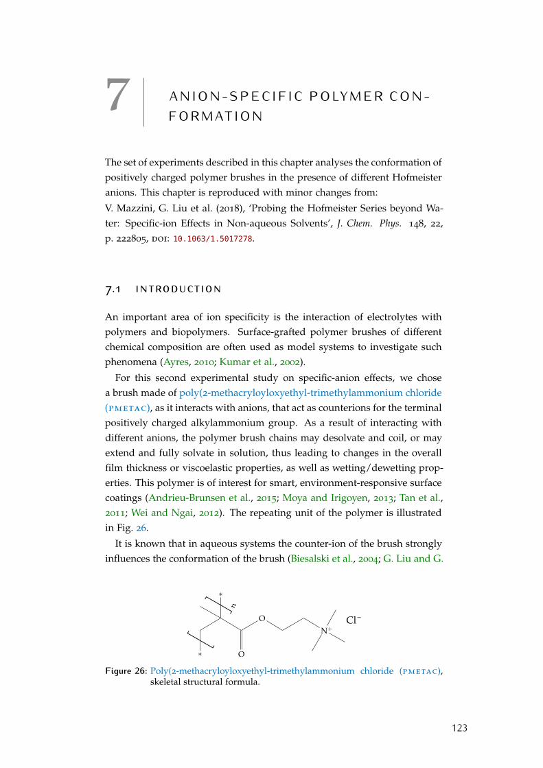
7 A N I O N -S P E C I F I C P O LY M E R C O N -F O R M AT I O N
The set of experiments described in this chapter analyses the conformation ofpositively charged polymer brushes in the presence of different Hofmeisteranions. This chapter is reproduced with minor changes from:
V. Mazzini, G. Liu et al. (2018), ‘Probing the Hofmeister Series beyond Wa-ter: Specific-ion Effects in Non-aqueous Solvents’, J. Chem. Phys. 148, 22,p. 222805, doi: 10.1063/1.5017278.
7.1 introductionAn important area of ion specificity is the interaction of electrolytes withpolymers and biopolymers. Surface-grafted polymer brushes of differentchemical composition are often used as model systems to investigate suchphenomena (Ayres, 2010; Kumar et al., 2002).
For this second experimental study on specific-anion effects, we chosea brush made of poly(2-methacryloyloxyethyl-trimethylammonium chloride(pmetac), as it interacts with anions, that act as counterions for the terminalpositively charged alkylammonium group. As a result of interacting withdifferent anions, the polymer brush chains may desolvate and coil, or mayextend and fully solvate in solution, thus leading to changes in the overallfilm thickness or viscoelastic properties, as well as wetting/dewetting prop-erties. This polymer is of interest for smart, environment-responsive surfacecoatings (Andrieu-Brunsen et al., 2015; Moya and Irigoyen, 2013; Tan et al.,2011; Wei and Ngai, 2012). The repeating unit of the polymer is illustratedin Fig. 26.
It is known that in aqueous systems the counter-ion of the brush stronglyinfluences the conformation of the brush (Biesalski et al., 2004; G. Liu and G.
∗
∗ O
O
N+[]
n
Cl–
Figure 26: Poly(2-methacryloyloxyethyl-trimethylammonium chloride (pmetac),skeletal structural formula.
123

124 anion-specific polymer conformation
Zhang, 2013). Azzaroni et al. (2005) studied the ion-specific properties andbehaviour of positively charged pmetac brushes in water. They showed,by coupling qcm with atomic force microscopy, infrared spectroscopy andcontact angle measurements, that pmetac brushes in water undergo totalcollapse in the presence of ClO4
– . The response of pmetac brushes in waterto Hofmeister anions and cations has been characterised in detail by Kou, J.Zhang, Wang et al. (2015), who found that the Hofmeister anions interactwith the charged sites on the brush to different degrees, in agreement withthe lmwa (Section 4.4), which is consistent with the expectations based ondispersion interactions.
7.2 Qcm for investigating polymer conformationA quartz crystal microbalance (qcm) is a surface-acoustic-wave-based ana-lytical instrument (Johannsmann, 2015) that employs a quartz crystal reson-ator to detect mechanical and rheological changes in its environment. Forexperiments in solution this could be a change in the solvent, adsorption ordesorption of material from the sensor surface or a change in conformationof molecules on the sensor surface.
The term ‘microbalance’ was introduced by Günter Sauerbrey (Sauerbrey,1959). Although the name implies that the qcm is a device for measuringsmall (micro) masses, it actually measures an areal mass density in the unitsof mass per unit area. Fundamentally, the qcm is a stress balance, in that itdetects periodic stresses exerted at its surface (Johannsmann, 2015).
7.2.1 Description of the technique
As crystalline quartz is piezolectric (that is, it generates an internal electricalcurrent when mechanically deformed by an applied force), its acoustic res-onance can be excited electrically (inverse piezoelectricity).
Whilst the main application of quartz resonators are in time and frequencycontrol (i.e. quartz clocks, computer clock signal), the fact that the resonancefrequency and resonance bandwidth depend on the environment the reson-ator is in contact with makes them suitable to be employed as frequency-based sensors.
The quartz crystal resonators we use are 330µm thick, 15mm diameterdisks with a fundamental resonance frequency of 5MHz, that have elec-trodes on both their faces in order to provide electrical contact. The crys-tal cut is chosen so that, when an ac-voltage is applied to the electrodes,an oscillating shear deformation is produced in the crystal (at-cut, that os-cillates in thickness-shear mode). If the frequency of the exciting voltage
7.2 Qcm for investigating polymer conformation 125
matches one of the acoustic resonance frequencies of the disk, the amplitudeof oscillation is large and the sensor draws a large electric current from thegenerator. The resonance frequencies are therefore easily found by scanningdifferent input voltage frequencies and measuring the current drawn by theelectrodes.
In the apparatus I employed, the quartz resonator is mounted on an O-ring so that it seals one side of a liquid sample cell. Only one face of thesensor is exposed to the sample cell environment.
It is crucial for surface-sensing in liquids that the resonator vibrates inshear-mode. A different oscillation where the disk expands would producecompressional waves. Compressional waves interact with liquid samplesmuch differently: whereas shear waves rapidly decay in liquids and in gases(according to Johannsmann (2015), the penetration depth at 5MHz in wateris 250nm), compressional waves propagate into fluids, and can be reflectedand scattered by objects in the sample cell and return to the sensor sur-face. This means that information from the liquid bulk is mixed with thesignal from the liquid at the sensor interface, and therefore the sensor doesnot just ‘see’ the fluid at its surface but well beyond that, therefore losing itssurface-detection specificity. Compressional waves are a much more promin-ent problem in liquids than in gases because the latter have a low impedanceto compressional waves. As some flexural vibrating modes cannot be elim-inated form the resonator vibration because of energy trapping, efforts aremade so that the effects of compressional waves are constant and thereforeignored when looking at frequency shifts.
The quartz sensor resonance frequency fn and half-bandwidth Γn can beinterrogated in different ways (Johannsmann, 2015), that are based either onoscillator circuits, impedance analysis, or ring-down techniques. The instru-ment used in this work employs the ring-down technique: a radio frequency(rf) pulse of frequency close to the expected sensor resonance frequency isused to excite the quartz sensor; the excitation is then shut off and the cur-rent produced by the free decay of the sensor oscillation is recorded. Thesignal is fitted by a decaying cosine function in time: the decay time, whichis the time when the oscillations envelope has decayed by a factor of e, isequal to (1/2πΓn); the cosine period is equal to 1/fn. This technique is atthe base of the patented quartz crystal microbalance with dissipation mon-itoring (qcm-d) from Q-sense, used here: ‘-D’ stands for ‘with dissipationmonitoring’, and the dissipation factor is defined as Dn = 2Γn/fn. The ring-down method can be faster than the other interrogation techniques. Thismethod is analogous to the nmr free-induction decay, although they are dif-ferent in that the ring-down method uses a narrow rf pulse to excite onlythe resonant crystal oscillation mode of interest, whereas in nmr a broaderpulse is used to excite all of the different Larmor frequencies of the same

126 anion-specific polymer conformation
nucleus, that change based on its chemical environment. As this is not thecase in qcm, it is more efficient to excite the resonance frequency of interestand repeat the process for the overtones, than to excite all of the crystalresonances at once and decompose them by Fourier transform.
The changes in the sensor environment can be therefore detected as bothits resonant frequency, fn, and its dissipation factor, Dn, shifts from the ‘nat-ural’ ones. The first observable is sensitive to the stress at the sensor surface(which, if the situation satisfies certain conditions, is equivalent to the area-averaged mass per unit area); the second observable is instead related to thedamping properties (the viscous dissipation) at the sensor surface.
As the fundamental mode of the quartz-crystal disks with keyhole-shapedelectrodes (which are the type employed here) often behaves differently fromthe overtones — for reasons that are poorly understood (possibly poor en-ergy trapping), only the overtones are usually considered. These crystals arealso called overtone crystals for this reason.
7.2.2 Polymer conformation monitoring
So how can a qcm be used to monitor the conformation of polymer brushes?
A polymer brush is grafted to the gold electrode surface of the quartzsensor. The resonant frequency fn, and the energy dissipation Dn, are recor-ded continuously. We typically use the third overtone as the first overtoneis susceptible to drift, likely associated with the mounting of the resonatoror the keyhole- shaped electrodes. When measuring in liquids, the loadsensed by the resonator is not just the load of the polymer chains graftedto the surface, but also includes the mass of any solvent that is coupled toit (Craig and Plunkett, 2003). In systems like the one employed here, wherea polymer film is covalently bound to the sensor, the mass of the film cannotchange, but the coupled load can change in response to the configuration ofthe polymer and/or changes in the solvent.
Therefore, a swelling and solvation of the brush will produce a decreasein fn (increased load due to coupling with the solvent that enters the brush)and an increase in Dn (increased dissipation of the extended and solvatedpolymer chains. When the brush collapses and desolvates, the oppositehappens: less solvent is coupled to the brush, resulting in a positive ∆fn anda negative ∆Dn.
7.3 experiment detailsA Biolin Scientific Q-sense E1 qcm-d was used to measure the shifts in fre-quency (∆fn) and dissipation (∆Dn) of the polymer brush-coated resonator
7.3 experiment details 127
in the presence of 10−3molkg−1 electrolyte solutions (varying by anion) inthe solvents of interest. The preparation of the samples is described in Chap-ter 5.
7.3.1 pmetac brush preparation
This procedure was performed by the group of Prof. Guangming Liu at theDepartment of Chemical Physics, Hefei National Laboratory for PhysicalSciences at the Microscale, University of Science and Technology of China,Hefei, P. R. China. I received the sensors ready for qcm use.
The gold-coated resonators used in the qcm-d were cleaned by piranhasolution (volume fractions ϕH2O2 = 0.3, ϕH2SO4 = 0.7) for 10min at 60 ◦C,then rinsed with copious amounts of ultra-pure water, and dried undera nitrogen stream before use. The clean resonators were immersed in a5× 10−3moldm−3 solution of mubb (ω-Mercaptoundecyl bromoisobutyra-te) in anhydrous ethanol for ≈ 24h at room temperature to form a uniformmonolayer of initiator with a thickness of ≈ 1.2nm, as determined by ellip-sometry. Pmetac brushes were prepared using the si-atrp method (Ed-mondson et al., 2004). Typically, metac (2-methacryloyloxyethyl-trimethyl-ammonium chloride) (5.94 g, 2.86× 10⁻²mol), the free initiator 2-ebib (e-thyl 2-bromoisobutyrate) (2.7× 10⁻² g, 1.4× 10⁻⁴mol), and bpy (2,2’-dipyri-dyne) (4.4× 10⁻² g, 2.8× 10⁻⁴mol) were dissolved in 20ml of meoh/watermixture (ϕMeOH = 0.8, ϕH2O = 0.2). Then, the initiator-modified substrateswere placed inside the flask, and the solution was stirred at 25 ◦C under ar-gon for 120min to remove dissolved oxygen. Afterward, CuBr (2× 10⁻² g,1.4× 10−4mol) and CuBr2 (3× 10⁻³ g, 1.4× 10⁻⁵mol) were quickly addedunder argon protection at 25 ◦C. The polymerization was allowed to pro-ceed for a specific time to prepare the pmetac brushes. At the end of poly-merization, the resonators grafted with pmetac brushes were washed withwater and meoh, and then soaked in a meoh/water mixture (ϕMeOH = 0.8,ϕH2O = 0.2) overnight to remove the ligand and unreacted monomer.
7.3.2 Experiment setup and procedure
The ‘bare’ sensor was a QSensor QSX 301 Gold 5MHz quartz crystal reson-ator. The polymer brush was constituted by pmetac.
I used two different pmetac-coated sensors for our measurements, asthe first deteriorated after some time. The dry thickness of the brush was31.11nm for the first sensor (used for meoh, fa and dmso) and 28.69nmfor the second one (used for dmso, pc and water).
In order to avoid contamination, special high-chemical resistance O-ringsand gaskets were used.
128 anion-specific polymer conformation
An ISMATEC REGLO Digital ISM596 peristaltic pump was connected tothe outlet tubing of the qcm sample chamber to draw the solution from thestorage vial into the measuring cell via the ptfe inlet tubing of the cell. Thisconnecting order was chosen as the sample would only come in contact withTeflon® tubing before entering the measurement cell, and therefore possiblecontamination by coming in contact with the pump tubing was avoided.
All of the solvent exchange in the cell was performed at a pumping rate of0.1mlmin−1, to avoid disturbing the brush conformation or inducing stresson the O-ring. The pump was stopped after each liquid exchange.
The vial containing the sample (or solvent) that was being sampled had tostay uncapped for the whole duration of the operation, as the feeding tubingto the sample cell had to be immersed inside the vial. In order to limit theexposure of the solutions to atmospheric moisture, the opening of the vialwas covered with aluminium foil and sealed with Parafilm M® on top of thefoil. In addition, the samples were only taken out of the storage desiccatorsfor the time necessary to perform a measurement.
The measuring procedure was as follows: the baseline in pure solvent wasacquired for at least 30min (no solvent flow); 1ml of the electrolyte solutionwas pumped into the chamber and left to equilibrate for at least 30min; 5mlof the neat solvent was pumped through the cell to rinse the cell, and thisoperation was repeated until the baseline was reached again.
This procedure was performed for each electrolyte both on the brush-coated sensor and on the bare sensor. Each electrolyte measurement wasrepeated for confirmation.
Difficulties were encountered, especially in solvents where the brush re-sponse was small: in fa a strong baseline drift was observed, and in dmsothe presence of bubbles rendered the acquisition problematic, creating theneed for many repeated runs.
7.3.3 Correcting for solution density and viscosity effects
As the viscosity and density of an electrolyte solution vary depending onthe concentration and type of electrolyte, the resonant frequency and dis-sipation of the quartz resonator will be affected by changes in the solution.As a result, the measured ∆fn and ∆Dn relative to the neat solvent, includeboth the signal of interest (changes in brush conformation in response to theelectrolyte) and the response to the altered properties of the solution. The ef-fect of NaBr concentration on the blank sensor in different solvents is shownin Fig. 27. The effect increases with concentration of the salt as expected, asthe viscosity and density of the solutions increase, but the slopes differ bysolvent and dmso and fa are the ones showing the most dramatic increase.

7.3 experiment details 129
DMSO
FA
H2OMeOH
−∆F3 = 336m2 − 2.16, r2 = 0.9963
−∆F3 = 256m2 + 1.11, r2 = 0.9995
−∆F3 = 26m2 + 0.2, r2 = 0.9992
−∆F3 = 93m2 − 0.65, r2 = 0.9937
0
10
20
30
40
50
60
70
80
0.01 0.05 0.10 0.15 0.20 0.30
m/(molkg−1)
−∆F3/(Hz)
DMSO
FA
H2O
MeOH
∆D3 = 136m2 − 0.823, r2 = 0.9956
∆D3 = 101m2 + 0.511, r2 = 0.9997
∆D3 = 10m2 + 0.011, r2 = 0.9993
∆D3 = 38m2 − 0.412, r2 = 0.9939
0
5
10
15
20
25
30
0.01 0.05 0.10 0.15 0.20 0.30
m/(molkg−1)
106∆D
3
Figure 27: Effect of NaBr solutions at different concentrations on the shifts meas-ured by the bare quartz resonator. The shadings around the fitting linesrepresent a 95% confidence interval. The normalised frequency shift ∆F3is plotted rather than ∆f3, and the frequency shift axis is reversed.
No correlation with the solvent density or compressibility is apparent. Pcwas not tested due to the low solubility of NaBr in this solvent.
Please note that, in all the plots showing qcm results, the y-axis of thefrequency shift plot has been reversed, so that the frequency and the dissip-ation shift have the same sign when the polymer brush swells or collapses(positive shift for swelling, negative shift for collapse). In addition, the nor-malised frequency shift ∆F3 is plotted rather than ∆f3.
In order to isolate the response of the film, the ∆fn and ∆Dn caused bythe same solution on a blank sensor were recorded and subtracted fromthe shifts measured in the presence of the polymer brush. This correctionmethod is simplistic as it assumes the effects to be additive, but it is a simpleand accessible way of estimating the change in sensor environment. Fig-ure 28 shows both the brush-coated sensor and the bare sensor shifts inthe presence of the different 10−3molkg−1 electrolytes, and demonstrates aclear distinction between the two responses.
7.3.4 Choice of the electrolyte sample concentration
The net response of the pmetac brush to solutions at different concentra-tions of NaBr (this experiment is not anhydrous) is plotted in Fig. 29. Increas-ing concentrations of salt do not have a marked effect on the response mag-nitude of the brush. A low electrolyte concentration was therefore chosenfor the experiments in order to avoid saturating the brush response.

130 anion-specific polymer conformation
water
methanol
formam
idedim
ethylsulfoxidepropylene
carbonate
NaBrNaCl NaClO4NaI NaSCNNaOAc NaF
−40−30−20−100102030405060
−100−80−60
−40−200
20
40
−14−12−10−8−6−4−20246
0123456789
0102030405060708090
electrolyte
−∆F3/(Hz)
water
methanol
formam
idedim
ethylsulfoxidepropylene
carbonate
NaBrNaCl NaClO4NaI NaSCNNaOAc NaF
−25−20−15−10−505101520
−20
−15
−10
−5
0
5
−5
−4
−3
−2
−1
0
1
−1.5−1.0−0.50.00.51.01.52.02.53.03.5
0
5
10
15
20
25
electrolyte
106∆D
3
Figure 28: Comparison of shifts recorded in presence of the brush-coated sensor(full circles) and the bare quartz sensor (empty triangles). This showsthe significance of the brush signal. The normalised frequency shift ∆F3is plotted rather than ∆f3, and the frequency shift axis is reversed.
−100
−90
−80
−70
−60
−50
−40
−30
−20
−10
0
0.01 0.05 0.10 0.15 0.20
m/(molkg−1)
−∆F3/(Hz)
−35
−30
−25
−20
−15
−10
−5
0
0.01 0.05 0.10 0.15 0.20
m/(molkg−1)
106∆D
3
Figure 29: Effect of different concentrations of NaBr on the net pmetac shifts inmeoh. The normalised frequency shift ∆F3 is plotted rather than ∆f3,and the frequency shift axis is reversed.

7.4 results and discussion 131
swel
lin
gco
lla
pse
FA
water
DMSO
PC
MeOH−150
−100
−50
0
50
0 100 200 300 400 500 600 700 800
time/min
−∆F3/(Hz) sw
elli
ng
coll
aps
e
FA
water
DMSO
PC
MeOH−30
−25
−20
−15
−10
−5
0
5
10
15
20
25
0 100 200 300 400 500 600 700 800
time/min
106∆D
3
Figure 30: Comparison of the effect of 10−3molkg−1 NaClO4 on the pmetacbrush in different solvents. The corresponding conformational changeof the brush is indicated on the plots. The blue arrows indicate whenthe pure solvent has been flushed. The normalised frequency shift ∆F3 isplotted rather than ∆f3, and the frequency shift axis is reversed.
7.4 results and discussion
The effects of water contamination on the sie polymer conformations arediscussed in Appendix F.2. These are found to be more relevant for ‘chao-tropic’ ions; however, the overall sie trend is not altered.
7.4.1 Effect of NaClO4 on pmetac in different solvents
As an exemplification of the recorded brush response, Fig. 30 shows theqcm recording of the frequency and dissipation shifts of the pmetac brushwhen a 10−3molkg−1 solution of NaClO4 is introduced in the sample cell.I have selected this electrolyte because the brush displays the most extremesolvent-response: its conformation is dramatically different in magnitudeand sign, and collapse is observed in protic solvents while swelling happensin aprotic ones. The response observed in water is in agreement with literat-ure results (Azzaroni et al., 2005; Kou, J. Zhang, Wang et al., 2015).
In meoh, the brush does not re-swell when neat solvent is flushed intothe cell (neat solvent application indicated by the arrows in Fig. 30). Theexchange with different counterions was necessary in order for the brushto be swollen in neat meoh. Also the kinetics of the brush response (timeneeded to return to the baseline signal after the brush deformation) changesdepending on the solvent, with it being the slowest in pc and water.

132 anion-specific polymer conformation
7.4.2 Discussion of results in all solvents
The monitoring by qcm of the conformation of a brush grafted to a quartzcrystal resonator can be interpreted as follows: if the oscillation frequencyincreases(loss in coupled mass) and the dissipation decreases (coupled massdecreasing), the brush is collapsing. If the opposite is observed, the brushis swelling with respect to its status in the neat solvent. The swelling of thebrush has been justified as resulting from the ingress of external counterionsinto the brush, that break up the multiplets formed by the ion-pairs, thatpartly restrict the full stretching of the polymer chains (Chu et al., 2014).Multiplets are aggregates of ion pairs (e.g. 2 ion pairs or 3 ion pairs), thatform in consequence of the presence of densely confined charges. The brushinstead collapses because of direct anion-specific binding to the alkylam-monium groups and neutralisation of the net charge (Azzaroni et al., 2005).
The results of the qcm measurements are summarised in Fig. 31. Here∆F3 and ∆D3 provide for a consistent picture of how ions influence theconformation of the pmetac polymer film in different solvents. The ions areordered according to the fundamental series for anions (i.e. the Hofmeisterseries). It is clear that the protic solvents, water, meoh and fa all exhibitsie that follow the Hofmeister series. The series is reversed in the aproticsolvents dmso and pc.
In fa and dmso, the effects of the electrolytes are smaller compared tothe other solvents. The pmetac polymer brush carries a positive chargethrough the dissociation of the chloride cation from the alkylammoniumgroups. These charged groups promote the swelling of the film. Thereforea collapse of the film is associated with a decrease in the overall positivecharge due to incorporation of anions into the film. Conversely swelling ofthe film infers an increase in the positive charge or osmotic pressure in thefilm associated with ingress of kosmotropic anions into the brush. The latterrequires that the kosmotropic anions do not form contact ion pairs with thealkylammonium groups of the brush (Kou, J. Zhang, Z. Chen et al., 2017).
7.4.3 ∆D versus −∆F plot
In order to investigate changes in the viscoelastic properties of the brush, aplot of ∆D3 versus −∆F3 can be constructed for all the electrolytes in thedifferent solvents. This is shown in Fig. 32. To a good approximation, thepoints form a line of constant slope, indicating that the electrolytes do notsubstantially alter the viscoelasticity of the brush.

7.4 results and discussion 133
collapseswelling
collapseswelling
collapseswelling
collapseswelling
swelling
water
methanol
formam
idedim
ethylsulfoxidepropylene
carbonate
NaBrNaCl NaClO4NaI NaSCNNaOAc NaF
−25
0
25
50
−100
−50
0
50
−10
0
−3
0
3
6
0
25
50
75
electrolyte
−∆F3/(Hz)
swellingcollapse
swellingcollapse
swellingcollapse
swellingcollapse
swelling
water
methanol
formam
idedim
ethylsulfoxidepropylene
carbonate
NaBrNaCl NaClO4NaI NaSCNNaOAc NaF
−20
−10
0
10
20
−20
−10
0
−6
−4
−2
0
−3
−2
−1
0
1
2
0
5
10
15
20
25
electrolyte
106∆D
3
Figure 31: Summary of frequency and dissipation shifts produced by a10−3molkg−1 electrolyte solution on a pmetac brush in different sol-vents. The corresponding conformational change of the brush is indic-ated on the plots. In meoh, the electrolytes NaOAc and NaClO4 havenot been measured in anhydrous conditions. For NaOAc, the value from‘as supplied’ meoh has been used and is represented by the empty tri-angle symbol. NaClO4 has not been tested in dry conditions as the brushis difficult to re-swell afterwards, as seen by our non-anhydrous tests.The value is an estimate calculated from the non-anhydrous NaClO4measurement by using the ratio of the anhydrous to non-anhydrous re-sponse of NaSCN, and is indicated by a square symbol. The normalisedfrequency shift ∆F3 is plotted rather than ∆f3, and the frequency shiftaxis is reversed.

134 anion-specific polymer conformation
NaBr
NaCl
NaClO4
NaI
NaSCN NaBr
NaCl
NaClO4
NaI
NaOAc
NaSCN
NaBr
NaCl
NaClO4
NaF
NaI
NaOAc
NaSCNNaBr
NaCl
NaClO4
NaF
NaI
NaOAc
NaSCN
NaClO4
NaI
NaSCN
−20
−10
0
10
20
−100 −50 0 50
−∆F3/(Hz)
106∆D
3
solventDMSOFH2OMeOHPC
swelling
collapse
maximumcollapse
Figure 32: ∆D3 versus −∆F3 plot of the electrolytes in all of the solvents investig-ated. The normalised frequency shift ∆F3 is plotted rather than ∆f3, andthe frequency shift axis is reversed.
7.5 summaryIn this chapter, the conformation of polymer brushes has been successfullyinvestigated by qcm measurements. The ion-specific brush response to thedifferent Hofmeister anions depends on the solvent environment: water,meoh and fa display a forward Hofmeister series; dmso and pc a reverseHofmeister series.
Also this experiment shows that the solvent affects the manifestation of thefundamental Hofmeister trend for anions, causing an inversion exactly as isobserved in the sec experiments. In this case though, the watershed solventis shifted from fa (which was the ‘neutral’ solvent in sec measurements):the series in fa is still a Hofmeister one.
The surfaces interacting with the system are very different in these twoexperiments, with Sephadex® being covered in OH groups and largely neutral(a very small quantity of the hydroxyls can be expected to dissociate andbecome negatively charged), whereas pmetac carries a net positive chargeon an alkylammonium group. Despite the large difference in the surfaceproperties and net charge, the Hofmeister series is observed in practicallyall cases, and a reversal happens in both experiments. This is remarkableagreement.
It is best to discuss the sie trends measured here in conjunction with thesec trends of Chapter 6, in order to analyse the connection of the experimentseries with the solvent properties in a global perspective. Such treatment isperformed Section 8.2.
8 A N O V E R A L L V I E W O F A N I O NT R E N D S I N N O N - A Q U E O U S S O L-V E N T S
The findings from the previous chapters are here discussed to form a gen-eral picture of sie in non-aqueous solvents. The experiment results requirededicated attention and I will discuss the general implications of these in Sec-tion 8.2, which is is reproduced with changes from:
V. Mazzini, G. Liu et al. (2018), ‘Probing the Hofmeister Series beyond Wa-ter: Specific-ion Effects in Non-aqueous Solvents’, J. Chem. Phys. 148, 22,p. 222805, doi: 10.1063/1.5017278.
8.1 a global depiction of sie in non-aqueous sol-vents
The investigations presented in this thesis have struggled against: a limitedand patchy literature on sie in non-aqueous electrolytes, that rendered gen-eral considerations difficult to formulate; the intrinsic difficulties presentedby working in non-aqueous electrolytes; and the challenges in measuringa representative range of Hofmeister electrolytes, that includes difficultiesassociated with the solubilities of the electrolytes and the large number ofexperiments required to observe sie trends.
Despite those difficulties, a general qualitative description of the role ofthe solvent on sie is achieved, and the fundamental understanding of sie isinformed by this work. Also, some rules of thumbs are proposed for the be-haviour of different non-aqueous electrolytes, depending on the conditionsand interacting species (presence of a surface, ion-ion interactions).
The succession of Chapters 3 to 7 takes in consideration systems at increas-ing levels of complexity in terms of interacting entities.
The initial literature review of Chapter 2 gathers very complex and experi-ment-dependent sie evidence. A number of important points emerge: sieare observed in all solvents, and they follow a variety of different series,including the Hofmeister and lyotropic ones. This shows that the Hofmeis-ter series is not exclusive to water. The absence of a clear overall patternindicates that a rich level of complexity is present, and therefore sie in non-aqueous solvents are at least as many-sided as they are in water. Despitethe variability, there is evidence that the Hofmeister series and the reverse
135

136 an overall view
lyotropic series are the most frequent trends for anions and cations, respect-ively.
This hint is confirmed by the electrostriction studies of Chapter 3, where Ihave individuated the fundamental sie series for anions and cations: theseare the forward Hofmeister series for anions and the reverse lyotropic seriesfor cations. They are independent of the solvent, and are valid for infinitelydilute solutions and in the absence of interacting surfaces. Consequently, Iproposed the interpretation that the sie ordering is fundamentally a prop-erty of the ion, and, as one moves away from the ideal bulk conditions, theeffects of ion-ion interactions at real concentration, of ion-surface interac-tions in the presence of surfaces and of various experiment conditions (e.g.temperature) perturb the fundamental series. This is an important step for-ward in the interpretation of the general sie phenomenon, but at this pointa question still hangs unanswered. How do the perturbations act? That is,what are the dominant interactions (or properties) of the system that estab-lish a different perturbed order of the fundamental series?
A first step in answering this question is taken with the examination of thevolcano plots for non-aqueous solvents in Chapter 4. Starting with standardsolvation energies, the volcano trends appear broadly in all solvents, sug-gesting that the same interactions are at play and determine the ion-solventinteraction. This is remarkable given the widely different properties of therange of solvents examined, and consolidates the thesis of Chapter 3, that theions determine the fundamental ordering of sie. In addition, the data showthat, whereas the cation and anion trends observed in water can be expectedto hold for protic non-aqueous solvents, and the cation trends in water canbe expected to hold also in aprotic solvents, this prediction does not applyto anion trends in aprotic solvents. In this last case, one could expect perturb-ations and reversal as a result of the solvent change from hydrogen-bondingto non-hydrogen bonding. The extension of the volcano plots to real con-centrations (by studying non-aqueous activity coefficients and the solubilityof electrolytes) shows that the infinite dilution findings are generally con-firmed. This is important because the volcano plots at real-concentrationsalso take into account the cation-anion ‘matching’ effect. This study high-lights the limited ability of aprotic solvents to solvate anions, which revealscrucial for the appearance of solvent-related perturbations in volcano plots.In this study, no relevant interacting surfaces are present, but ion-ion inter-actions are, thus adding an additional level of detail to the non-aqueous siepicture.
The experimental work of Chapters 6 and 7 presents the highest com-plexity in the range of this thesis, as ion-solvent, ion-ion, and ion-interfacesinteractions are present. This allows to bring into focus the dominant inter-

8.1 a global depiction of sie in non-aqueous solvents 137
actions when interfaces are present: these are the dispersion contributions tothe surface-solvent-ion competition, as extensively discussed in Section 8.2.
The overall interpretation proposed in this thesis is therefore that sie arefundamentally a property of the ion, which follows the forward Hofmeisterseries for anions and the reverse lyotropic series for cations in ideal condi-tions, independently of the solvent. The interaction of ions with other ionsor with surfaces, and other changes from the ideal conditions act as perturb-ations to this fundamental series.
The rules of thumb that derive from the findings above can be summarisedas follows:
• for bulk properties of aqueous and non-aqueous electrolytes at infinitedilution, the fundamental series is to be expected (forward Hofmeisterfor anions and reverse lyotropic for cations);
• for bulk properties at real concentrations, the protic/aprotic nature ofthe solvent is the dominant characteristic that perturbs the anion series.The cation series is instead expected to be akin to that in water in bothprotic and aprotic solvents;
• for real concentrations and interacting surfaces, the dispersion inter-actions of both solvent and surface contribute to perturbing the funda-mental anion series. These can cause reversal of the series, and solventsof intermediate polarisability might not exhibit clear sie trends.
This provides a framework for understanding how ion-specific trends innon-aqueous solvents are related to ion-specific trends in water.
Another topic that I would like to touch upon is the role of the ‘structure’of the solvent. This is a property that is ill-defined (Ninham and Lo Nostro,2010), and extremely difficult to quantify experimentally. It also includesthe structuring due to the presence of a hydrogen-bonding network, but ithas a more general significance. That is, the electron distribution around asolvated ion will vary greatly from solvent to solvent, and consequently thepotential that the ion is experiencing, which includes many-body interac-tions and higher order multipole contributions. The topological distributionaround an ion in solution is challenging to investigate and is also the ul-timate challenge for theory and modelling. The debate is still active as tothe range to which the ions perturb the ordering of water molecules in solu-tion (Funkner et al., 2012; Gurau et al., 2004; Paschek and Ludwig, 2011).This has not been addressed in my work, but deserves to be included infuture investigations. On the other side, the fact that such general ion trendsare observed is definitely remarkable given the great difference in propertiesof the solvents investigated.
In addition, I have tested the influence of water as an impurity with sometargeted testing. I concluded that the presence of small quantities of wa-

138 an overall view
ter (< 0.2%) does not affect the sie trend in the non-aqueous solvents ex-amined, relatively to the experiments performed. I have collected evidence,though, that higher quantities of water influence the magnitude of sie innon-aqueous solvents and the peak shape in sec. This topic is a vast oneand it demands to be addressed in depth.
A number of authors have made remarks about the risk of looking toohard for a simple explanation of the universal sie trends. They note thatno isolated property of an ion or a surface can be turned into a master keyto unlock all the variations and manifestations of these phenomena (Kunz,2009; Okur et al., 2017). That is, the observed and quite universal qualitativeseries are actually the result of subtle balances of a number of very specificcompeting interactions. Therefore a qualitative analogy across a numberof experiments does not demonstrate that they are governed by the samerules. I hope that the general picture presented here does not come across asshoddy reductionism, as it is rather an attempt at organising this complexityin the broader context of non-aqueous solvents. I hope that the appreciationof the author for the detail and for the complexity of the sie phenomenais clear throughout this work. I also look forward to improvements of thepicture and interpretation presented.
The present work also highlights the need for additional targeted sie ex-periments in non-aqueous solvents, in order to further define the pictureintroduced here.
A final important point to note is that the findings presented show thatthe protagonist role that has been attributed to water for the manifestationof sie needs to be put into perspective. I have confirmed that sie are not anexclusive feature of aqueous solutions, and that other non-aqueous solventsshow the same trend. This is not to diminish the importance of water tohuman life, or to dismiss the intriguing charm of water — although I mightnot agree that it i s the most complex solvent, as stated in Kunz (2009), butrather the most extensively studied one. The usefulness and the allure ofinvestigating non-aqueous electrolytes, not just as a niche sector functionalto direct application, but as a broader knowledge horizon that has the poten-tial of furthering the understanding of fundamental scientific queries, showsthrough.
If sie are fundamental for enabling life processes, then could life basedon a non-aqueous solvent be possible? Might it already be happening on aremote planet in the galaxy?
And this ultimately circles back to the understanding of water, the mostimportant solvent for human existence.

8.2 the global experiment picture of anion trends 139
8.2 the global experiment picture of anion trendsThe meaning of the ion-specific non-aqueous trends presented in detail
in Chapters 6 and 7 are best discussed jointly with a general view.I have performed experiments investigating sie in two different systems
using the same range of solvents, to shed light onto the effects of interact-ing surfaces and real concentrations on the fundamental anion series (theHofmeister series, Fig. 1) individuated in Chapter 3.
The nature of the sec and qcm experiments is very different. In thechromatography experiments the interacting surface is a polar, largely un-charged, stationary phase, whereas in the qcm experiments a polymer brushterminated in cationic alkylammonium groups constitutes the interactingsurface. In addition, in sec a dynamic property is evaluated, whereas theqcm experiment can be considered a static one. Despite the differencesbetween these experiments, the trends in the sie are consistent, as Table 29illustrates.
Table 29: Summary of the anion-specific trends from experiment
experiment water meoh fa dmso pc
sec HS HS no trend R-HS R-HSqcm HS HS HS R-HS R-HS
In almost the totality of solvent-experiment combinations, the Hofmeisterseries manifests, either in a forward or reverse ordering. This is in broadagreement with the conclusions from Chapter 3, where the forward Hofmeis-ter series was identified as the fundamental series of anions in all solvents,for bulk properties of a solution at infinite dilution. However, a further de-gree of complexity is present here, compared to the fundamental Hofmeisterseries of Chapter 3: the series reverses in some solvents, and in one case noseries can be determined at all. This is an indication that interacting solvent,surfaces as well as ion-ion interactions play a substantial role in perturbingthe fundamental Hofmeister ordering. This additional degree of complexitywas similarly encountered in Chapter 4, where the trends in the thermody-namics of solvation were examined with the volcano plot treatment. There,solvent-related perturbations were observed in the manifestation of a vol-cano trend for the standard solvation energies of electrolytes in differentsolvents, and it was concluded that the anion trends observed in water canbe expected to be found unchanged in protic solvent, but not necessarilythus in aprotic solvents, where the order could be altered.
Taking a dichotomic view, and following the conclusions of Chapter 4, theexperiment results could be interpreted as follows: the fundamental series(forward Hofmeister) is observed in the protic solvents, whereas it is re-versed in the aprotic solvents. But this binary interpretation is an oversimpli-

140 an overall view
fication that does not fully capture the gradation of ion-specific behavioursdetected. In fact, in the qcm experiments the trend in fa followed the res-ults obtained in water and meoh (Fig. 31), whereas in the sec experimentsno clear trend was observed (Fig. 25). In addition, the amplitude of the brushresponse in the qcm experiment (Fig. 31) is large for water and meoh, issmaller for fa, is the smallest but reversed in dmso (where only two saltsare inducing a net variation of the brush conformation) and becomes largeagain and reversed in pc. This is not simply a direct-to-reverse Hofmeisterseries switch when passing from protic to aprotic solvents: a progression istaking place.
The aprotic solvents are considerably more polarisable than the protic sol-vents, with fa being the most polarisable protic solvent (Table 2). The resultscan therefore be interpreted as resulting from a competition between the sol-vent and the surface for the anion. The evidence suggests that in proticsolvents the more polarisable anions interact more strongly with the surface(and the less polarisable anions do not interact strongly with the surface),whereas in aprotic solvents the more polarisable anions do not interact withthe surface as they are more favourably solvated. It follows that the trendsobserved are not due to the binary categorisation of solvents into protic andaprotic ones, but rather reflect changes in the polarisability of the solvent.These findings show that a binary view of the behaviour of protic versusaprotic solvent with respect to ions is not capturing the full complexity ofthe phenomenon. Rather there is a gradation of behaviours, and the sur-face properties (both of the charged surface groups and the non-chargedsites) determine where the ‘watershed’ sits for the reversal of the observedtrend. In the two investigations performed here, the watershed is at fa whenSephadex® is the interacting surface, whereas it is at dmso when pmetacbrushes are the surface. It must also be noted that the type of experimentmay influence the observed trends.
The experimental observations can therefore largely be explained by anevaluation of the dispersion forces between the ions and the solvent and theions and the surface. Noting that these interactions will vary depending onthe nature of the surface. This suggests that for a different class of surface(e.g. a metal oxide) the series may well be reversed.
Thus the basis for which the huge complexity of sie observed across dif-ferent solvents and in the presence of different surfaces emerges: solvents ofdifferent polarisability are competing for ions of different polarisability withsurfaces that differ in polarisability and charge. This has the implicationthat, in order to model the sie in different solvents, the polarisability of thesolvent needs to be included, as the ion-solvent dispersion interactions playa fundamental role in sie.

8.2 the global experiment picture of anion trends 141
Table 30: Ionic ab initio static polarisabilties αi from Parsons and Ninham (2009).
anion αi/Å3
cation αi/Å3
F– 1.218 Li+ 0.028Cl– 4.220 Na+ 0.131Br– 6.028 K+ 0.795I– 8.967 Rb+ 1.348ClO4
– 4.790 Cs+ 2.354SCN– 7.428 (CH3)4N+ 7.448AcO– 5.607
In Chapter 4 I concluded that the anion series observed in water is lesslikely to be preserved in aprotic solvents than the cation series. A probablecause of the non-preservation of the anion trend appears now in light of theexperimental investigations: the dispersion interactions determined by thepolarisability of the solvent, surface, and ion. The fact that this perturba-tion is observed for anions but not for cations in Chapter 4 now falls intoplace: anions are more polarisable than the alkali metal cations (Table 30)and therefore the dispersion interactions are more relevant for this class ofions.
Furthermore, another cause of series reversal has been identified, beingsolvent polarisability. This adds to the list of other causes of reversal repor-ted in the literature: concentration, temperature, pH, counterion and surfacecharge (Lyklema, 2009; Parsons, Boström, Maceina et al., 2010; Robertson,1911; Schwierz, Horinek, Sivan et al., 2016; Senske et al., 2016). Notably,we have not encountered any other reports of the reversal of the anion seriesacross the solvents water, meoh, fa, dmso, pc, in the literature we reviewed(Table 13 of Chapter 2).
In view of these trends, a rule of thumb can be proposed: ion-specifictrends in weakly polarisable solvents can be expected to follow those ofwater, ion-specific trends in strongly polarisable solvents follow the reversetrend, whereas solvents of intermediate polarisability may not exhibit a cleartrend. Given the paucity of data on sie in non-aqueous solvents comparedto aqueous solvents, this rule of thumb may provide a useful starting pointfor engineering sie in non-aqueous solvents. As such the polarisability ofthe substrates should also be important in affecting sie trends and as suchmetal and metal oxide surfaces may well present different trends to thoseobserved here.
It must be noted, though, that polarisability and hydrogen-bonding prop-erties are different properties and are not connected by a simple relationship.I happened to use protic solvents of lower polarisability than the aprotic onesin my experiments. But there exist protic solvents of higher polarisabilitysuch as nma and t-buoh (Table 2) and aprotic solvents of low polarisabilitysuch as mecn and meno2. A first check of the rule of thumb here proposed

142 an overall view
is therefore apparent: to test the experimental ionic trends in protic solventof higher polarisability than fa and in aprotic solvents of lower polarisabil-ity than dmso. Especially the aprotic solvents of low polarisability will beimportant in confirming or disproving the importance of polarisability overhydrogen-bonding postulated here.
Further, the studies reported here all employed Na+ as the cation. It isknown in some ion-specific phenomena that the particular pairing of ions isimportant (Craig, Ninham et al., 1993a,b; Kunz and Neueder, 2009; Lyklema,2003). This aspect and the cation series per se in non-aqueous solvents havenot been investigated here and remain a challenge for future investigations.The division of sie in a cationic and anionic series is an artificial devicethat simplifies the organisation of the information, but has no real physicalmeaning as an ion cannot actually exist as an isolated charge. Therefore anion in solution will also be affected by its counterion.
9 C O N C L U S I O N S
This thesis presents a wide-ranging investigation of specific-ion effects (sie)in non-aqueous solvents. This is a qualitative study of the ordering of sie innon-aqueous solvents compared to water. It consists of a comprehensive re-view of the literature, analysis and interpretation of a carefully selected sub-set of the literature data for non-aqueous electrolytes, and an experimentalinvestigation of sie in non-aqueous solutions.
In Chapter 1, I have clarified the terminology, that is particularly hazy inthis field: in order to do so, I have compiled the Hofmeister series for cationsand anions by merging the trends reported in a number of authoritative siereferences, and distinguished it from the lyotropic series, which is pertinentto a narrower category of sie.
The analysis starts with the review of the available literature on non-aqueous solvents in Chapter 2. A general account of the ordering of sieis compiled in different non-aqueous solvents. The results show the pres-ence of sie in non-aqueous solvents, which follow a variety of differentseries including the Hofmeister and lyotropic series, and display complexbehaviour such as series reversal. This shows that the Hofmeister series isnot a prerogative of aqueous solutions. In addition, no simple correlation ofthe ion-specific trend to the properties of the solvents is evident.
In Chapter 3 I have evaluated the standard electrostrictive volumes of Hof-meister electrolytes in a number of different solvents, and shown that, forbulk standard properties of electrolyte solutions, the sie ordering is inde-pendent of the solvent. I have therefore inferred that sie are fundamentallya property of ions, and that their universal fundamental ordering is the for-ward Hofmeister series for anions and the reverse lyotropic series for cations:
cations
anions
Li+ Na+ K+ Rb+ Cs+
F– Cl– Br– I– ClO –4 SCN–
this also evidences the fact that water is by no means a ‘special’ solventinvested of exclusive sie powers.
An additional literature data analysis is performed in Chapter 4, where Iextend the volcano plots of standard solvation energies to non-aqueous sol-vents. These are related to the law of matching water affinities (lmwa) prin-ciple. The volcano plot trends arise in both protic and aprotic non-aqueous
143

144 conclusions
solvents for cations, and in protic solvents for anions. I conclude that theevidence suggests that the ion size, rather than the ion-solvent interaction,is the origin of the volcano trend. This confirms the central role of the ionproperties for sie, presented in the previous chapter. Finally, I extendedthe volcano plots to real concentrations in water and non-aqueous solvents,confirming the standard volcano trends and proposed a rule of thumb forpredicting ion-specific trends in new systems, stating that, across solvents,the ion-specific trends observed in water will likely be observed in otherprotic non-aqueous solvents, and that the trends observed in water will bemore likely to hold for cations in non-aqueous solvents than for anions.
The experimental part of this thesis consists of two studies of the specific-anion effects in water and the non-aqueous solvents meoh, fa, dmso andpc. These tests particularly show how the trends are affected by the additionof an interacting surface. The first experiment is the size-exclusion chroma-tography (sec) of sodium Hofmeister electrolytes on a Sephadex® stationaryphase in the different solvents. I have found that, for the elution of elec-trolytes, water and meoh show a forward Hofmeister series, whereas dmsoand pc exhibit a reverse Hofmeister trend. No trend can be identified for fa.In the second set of experiments, I investigated the conformation (swelling/-collapse) of a cationic polymer brush in the presence of electrolyte solutionsin the same solvents. The ordering of anion effects follows a forward Hof-meister series for water, meoh and fa in this case, and a reverse Hofmeisterseries for dmso and pc. I have rationalised these experimental findingsby noting that the nuances of the behaviours in the different solvents bestcorrelate to the solvent polarisability. I have therefore concluded that disper-sion forces are crucial in the competition of the surface and the solvent forinteractions with the ions. These experiments are also the first reports of sieseries reversal due to the solvent.
In Chapter 8 I have discussed all the findings with a global view, assem-bling a coherent picture for the solvent effect in sie. Overall, I propose aninterpretation that places the fundamental origin of the sie on the ions, thatin ideal conditions (bulk properties and ion-solvent interactions only) followthe forward Hofmeister series for anions and the reverse lyotropic series forcations. The introduction of ion-ion interactions, interacting surfaces andso on can be consequently viewed as perturbations on these fundamentalseries. These are more likely to alter the fundamental (Hofmeister) orderingfor anions in aprotic solvents. Anions in protic solvents and cations in proticand aprotic solvents can instead be expected to more likely follow the order-ing observed in water. Finally, when interacting surfaces are present, theirperturbation effect can be largely rationalised by considering their polarisab-ility with respect to the solvent polarisability, as dispersion forces appear to

9.1 further work 145
present the crucial interaction that guides the ion preference for interactingwith either the solvent or the surface.
The information and data analysed here can serve as valuable testingground for the theories and models of sie, and strongly suggests that ‘ionsize’ and dispersion forces are the principal features in determining the ion-specific trends.
9.1 further workThe conclusions achieved in this thesis are based on as much evidence Icould gather. As I have pointed out, the conclusions and ideas presentedhere need to be further tested, and corrected, and refined. The avenues forfurther work are therefore abundant and span in all possible directions ofthe multifaceted world of non-aqueous electrolytes.
Experimentally, these include testing for the cation series in non-aqueoussolvents. When different cation trends at common anion are achieved, thesewill help in obtaining a picture for the trends depending on the cation-anionmatch.
In order to further understand how polarisability and proticity prevail,more solvents of different polarisability should be tested, and especiallyaprotic solvents of low polarisability.
Also, additional experiments involving different surfaces are useful. Inthese also the liquid-air interface is new ground to be probed, as well assurfaces with very different dielectric properties such as metals and mineraloxides. The study of the liquid-air interface presents a challenge as moistureneeds to be avoided.
Examples of possible experiments include spectroscopic and scatteringstudies, nmr studies, the self-assembly of surfactants, the solubility of gases.A list of experiments that I have attempted but have been unsuccessful isavailable in Appendix G.
On this note, also the influence of water on the sie needs to be studiedin more detail, as it could be particularly relevant in mixes with aproticsolvents.
Finally, the acquisition of more extensive fundamental thermodynamicdata as the molar electrolyte volumes, activity or osmotic coefficients of elec-trolytes is particularly needed to extend the base of electrolytes investigated.
This work has focussed on qualitative trends, but ultimately a more quant-itative treatment is required. Therefore, theoretical and modelling workshould be applied in order to develop a theory able to predict ion trendsfor water as well as non-aqueous electrolytes.

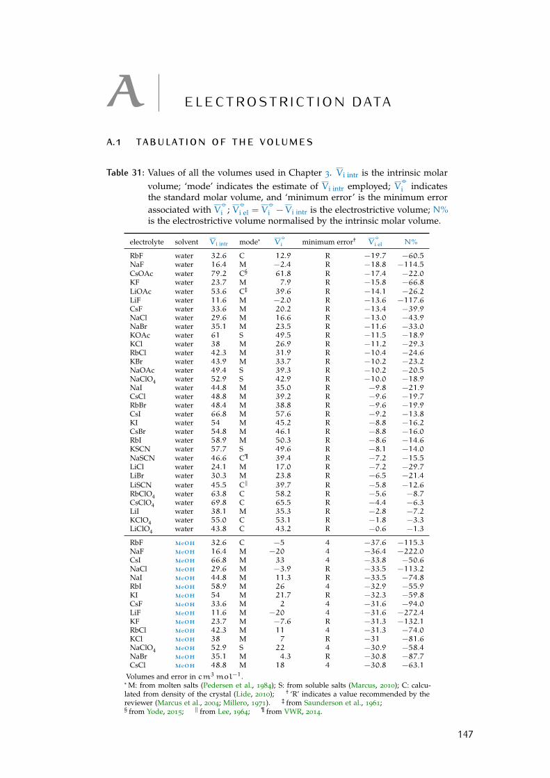
A E L E C T R O S T R I C T I O N DATA
a.1 tabulation of the volumesTable 31: Values of all the volumes used in Chapter 3. V i intr is the intrinsic molar
volume; ‘mode’ indicates the estimate of V i intr employed; V−◦i indicates
the standard molar volume, and ‘minimum error’ is the minimum errorassociated with V
−◦i ; V
−◦i el = V
−◦i − V i intr is the electrostrictive volume; N%
is the electrostrictive volume normalised by the intrinsic molar volume.
electrolyte solvent V i intr mode* V−◦i minimum error† V
−◦i el N%
RbF water 32.6 C 12.9 R −19.7 −60.5NaF water 16.4 M −2.4 R −18.8 −114.5CsOAc water 79.2 C§ 61.8 R −17.4 −22.0KF water 23.7 M 7.9 R −15.8 −66.8LiOAc water 53.6 C‡ 39.6 R −14.1 −26.2LiF water 11.6 M −2.0 R −13.6 −117.6CsF water 33.6 M 20.2 R −13.4 −39.9NaCl water 29.6 M 16.6 R −13.0 −43.9NaBr water 35.1 M 23.5 R −11.6 −33.0KOAc water 61 S 49.5 R −11.5 −18.9KCl water 38 M 26.9 R −11.2 −29.3RbCl water 42.3 M 31.9 R −10.4 −24.6KBr water 43.9 M 33.7 R −10.2 −23.2NaOAc water 49.4 S 39.3 R −10.2 −20.5NaClO4 water 52.9 S 42.9 R −10.0 −18.9NaI water 44.8 M 35.0 R −9.8 −21.9CsCl water 48.8 M 39.2 R −9.6 −19.7RbBr water 48.4 M 38.8 R −9.6 −19.9CsI water 66.8 M 57.6 R −9.2 −13.8KI water 54 M 45.2 R −8.8 −16.2CsBr water 54.8 M 46.1 R −8.8 −16.0RbI water 58.9 M 50.3 R −8.6 −14.6KSCN water 57.7 S 49.6 R −8.1 −14.0NaSCN water 46.6 C¶ 39.4 R −7.2 −15.5LiCl water 24.1 M 17.0 R −7.2 −29.7LiBr water 30.3 M 23.8 R −6.5 −21.4LiSCN water 45.5 C‖ 39.7 R −5.8 −12.6RbClO4 water 63.8 C 58.2 R −5.6 −8.7CsClO4 water 69.8 C 65.5 R −4.4 −6.3LiI water 38.1 M 35.3 R −2.8 −7.2KClO4 water 55.0 C 53.1 R −1.8 −3.3LiClO4 water 43.8 C 43.2 R −0.6 −1.3
RbF meoh 32.6 C −5 4 −37.6 −115.3NaF meoh 16.4 M −20 4 −36.4 −222.0CsI meoh 66.8 M 33 4 −33.8 −50.6NaCl meoh 29.6 M −3.9 R −33.5 −113.2NaI meoh 44.8 M 11.3 R −33.5 −74.8RbI meoh 58.9 M 26 4 −32.9 −55.9KI meoh 54 M 21.7 R −32.3 −59.8CsF meoh 33.6 M 2 4 −31.6 −94.0LiF meoh 11.6 M −20 4 −31.6 −272.4KF meoh 23.7 M −7.6 R −31.3 −132.1RbCl meoh 42.3 M 11 4 −31.3 −74.0KCl meoh 38 M 7 R −31 −81.6NaClO4 meoh 52.9 S 22 4 −30.9 −58.4NaBr meoh 35.1 M 4.3 R −30.8 −87.7CsCl meoh 48.8 M 18 4 −30.8 −63.1
Volumes and error in cm3mol−1.* M: from molten salts (Pedersen et al., 1984); S: from soluble salts (Marcus, 2010); C: calcu-lated from density of the crystal (Lide, 2010); † ‘R’ indicates a value recommended by thereviewer (Marcus et al., 2004; Millero, 1971). ‡ from Saunderson et al., 1961;§ from Yode, 2015; ‖ from Lee, 1964; ¶ from VWR, 2014.
147
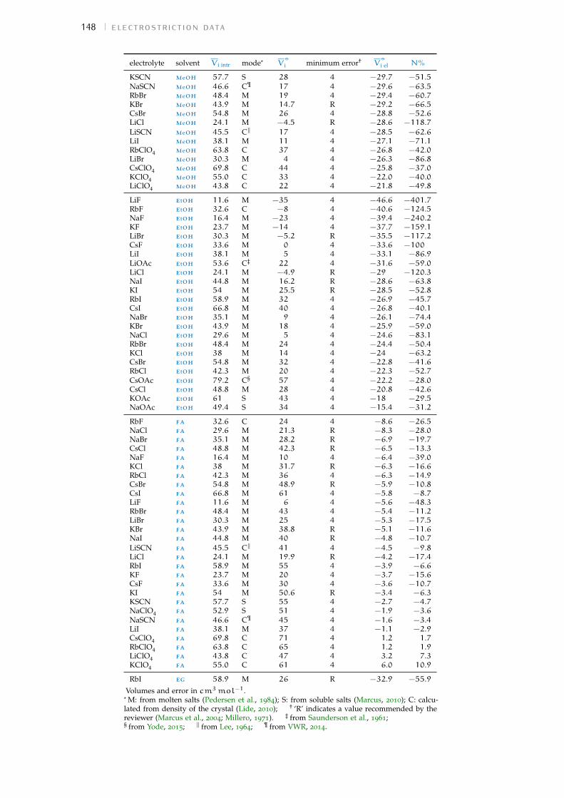
148 electrostriction data
electrolyte solvent V i intr mode* V−◦i minimum error† V
−◦i el N%
KSCN meoh 57.7 S 28 4 −29.7 −51.5NaSCN meoh 46.6 C¶ 17 4 −29.6 −63.5RbBr meoh 48.4 M 19 4 −29.4 −60.7KBr meoh 43.9 M 14.7 R −29.2 −66.5CsBr meoh 54.8 M 26 4 −28.8 −52.6LiCl meoh 24.1 M −4.5 R −28.6 −118.7LiSCN meoh 45.5 C‖ 17 4 −28.5 −62.6LiI meoh 38.1 M 11 4 −27.1 −71.1RbClO4 meoh 63.8 C 37 4 −26.8 −42.0LiBr meoh 30.3 M 4 4 −26.3 −86.8CsClO4 meoh 69.8 C 44 4 −25.8 −37.0KClO4 meoh 55.0 C 33 4 −22.0 −40.0LiClO4 meoh 43.8 C 22 4 −21.8 −49.8
LiF etoh 11.6 M −35 4 −46.6 −401.7RbF etoh 32.6 C −8 4 −40.6 −124.5NaF etoh 16.4 M −23 4 −39.4 −240.2KF etoh 23.7 M −14 4 −37.7 −159.1LiBr etoh 30.3 M −5.2 R −35.5 −117.2CsF etoh 33.6 M 0 4 −33.6 −100LiI etoh 38.1 M 5 4 −33.1 −86.9LiOAc etoh 53.6 C‡ 22 4 −31.6 −59.0LiCl etoh 24.1 M −4.9 R −29 −120.3NaI etoh 44.8 M 16.2 R −28.6 −63.8KI etoh 54 M 25.5 R −28.5 −52.8RbI etoh 58.9 M 32 4 −26.9 −45.7CsI etoh 66.8 M 40 4 −26.8 −40.1NaBr etoh 35.1 M 9 4 −26.1 −74.4KBr etoh 43.9 M 18 4 −25.9 −59.0NaCl etoh 29.6 M 5 4 −24.6 −83.1RbBr etoh 48.4 M 24 4 −24.4 −50.4KCl etoh 38 M 14 4 −24 −63.2CsBr etoh 54.8 M 32 4 −22.8 −41.6RbCl etoh 42.3 M 20 4 −22.3 −52.7CsOAc etoh 79.2 C§ 57 4 −22.2 −28.0CsCl etoh 48.8 M 28 4 −20.8 −42.6KOAc etoh 61 S 43 4 −18 −29.5NaOAc etoh 49.4 S 34 4 −15.4 −31.2
RbF fa 32.6 C 24 4 −8.6 −26.5NaCl fa 29.6 M 21.3 R −8.3 −28.0NaBr fa 35.1 M 28.2 R −6.9 −19.7CsCl fa 48.8 M 42.3 R −6.5 −13.3NaF fa 16.4 M 10 4 −6.4 −39.0KCl fa 38 M 31.7 R −6.3 −16.6RbCl fa 42.3 M 36 4 −6.3 −14.9CsBr fa 54.8 M 48.9 R −5.9 −10.8CsI fa 66.8 M 61 4 −5.8 −8.7LiF fa 11.6 M 6 4 −5.6 −48.3RbBr fa 48.4 M 43 4 −5.4 −11.2LiBr fa 30.3 M 25 4 −5.3 −17.5KBr fa 43.9 M 38.8 R −5.1 −11.6NaI fa 44.8 M 40 R −4.8 −10.7LiSCN fa 45.5 C‖ 41 4 −4.5 −9.8LiCl fa 24.1 M 19.9 R −4.2 −17.4RbI fa 58.9 M 55 4 −3.9 −6.6KF fa 23.7 M 20 4 −3.7 −15.6CsF fa 33.6 M 30 4 −3.6 −10.7KI fa 54 M 50.6 R −3.4 −6.3KSCN fa 57.7 S 55 4 −2.7 −4.7NaClO4 fa 52.9 S 51 4 −1.9 −3.6NaSCN fa 46.6 C¶ 45 4 −1.6 −3.4LiI fa 38.1 M 37 4 −1.1 −2.9CsClO4 fa 69.8 C 71 4 1.2 1.7RbClO4 fa 63.8 C 65 4 1.2 1.9LiClO4 fa 43.8 C 47 4 3.2 7.3KClO4 fa 55.0 C 61 4 6.0 10.9
RbI eg 58.9 M 26 R −32.9 −55.9
Volumes and error in cm3mol−1.* M: from molten salts (Pedersen et al., 1984); S: from soluble salts (Marcus, 2010); C: calcu-lated from density of the crystal (Lide, 2010); † ‘R’ indicates a value recommended by thereviewer (Marcus et al., 2004; Millero, 1971). ‡ from Saunderson et al., 1961;§ from Yode, 2015; ‖ from Lee, 1964; ¶ from VWR, 2014.
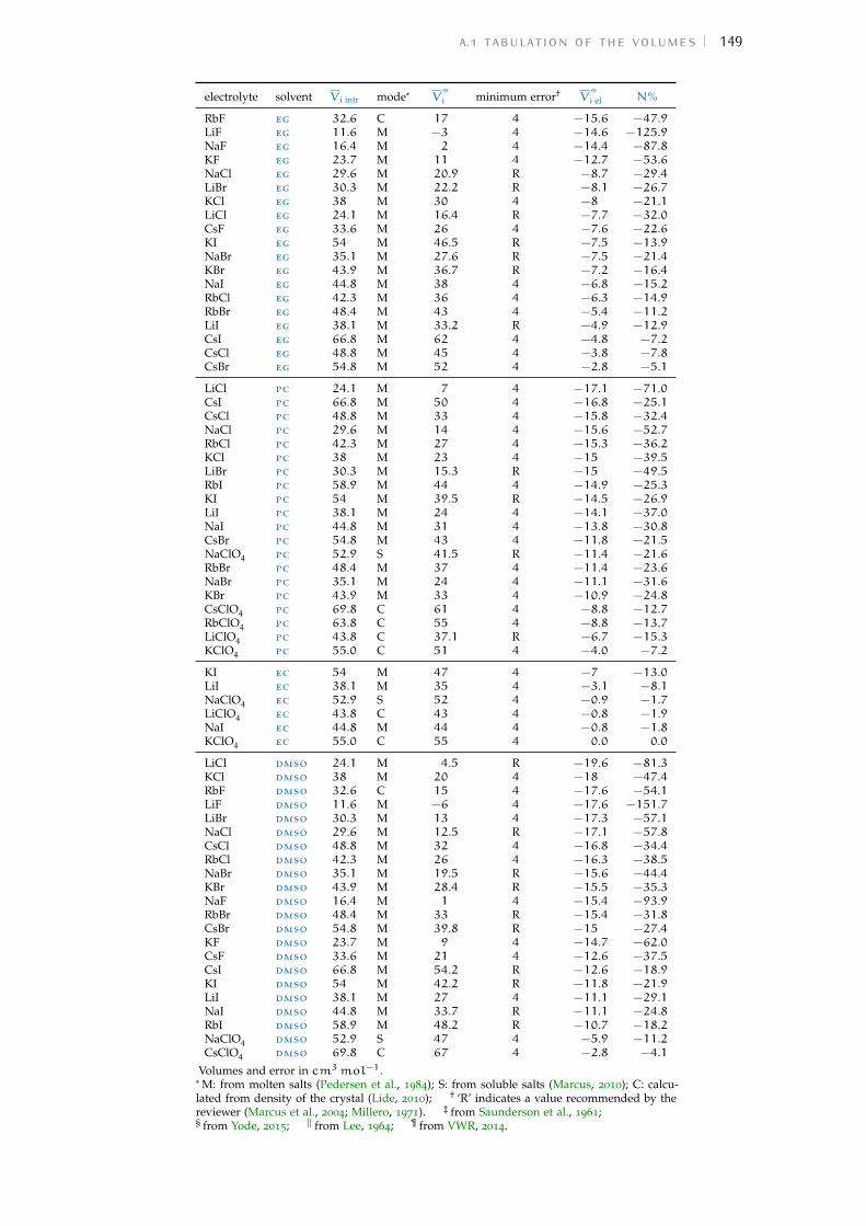
a.1 tabulation of the volumes 149
electrolyte solvent V i intr mode* V−◦i minimum error† V
−◦i el N%
RbF eg 32.6 C 17 4 −15.6 −47.9LiF eg 11.6 M −3 4 −14.6 −125.9NaF eg 16.4 M 2 4 −14.4 −87.8KF eg 23.7 M 11 4 −12.7 −53.6NaCl eg 29.6 M 20.9 R −8.7 −29.4LiBr eg 30.3 M 22.2 R −8.1 −26.7KCl eg 38 M 30 4 −8 −21.1LiCl eg 24.1 M 16.4 R −7.7 −32.0CsF eg 33.6 M 26 4 −7.6 −22.6KI eg 54 M 46.5 R −7.5 −13.9NaBr eg 35.1 M 27.6 R −7.5 −21.4KBr eg 43.9 M 36.7 R −7.2 −16.4NaI eg 44.8 M 38 4 −6.8 −15.2RbCl eg 42.3 M 36 4 −6.3 −14.9RbBr eg 48.4 M 43 4 −5.4 −11.2LiI eg 38.1 M 33.2 R −4.9 −12.9CsI eg 66.8 M 62 4 −4.8 −7.2CsCl eg 48.8 M 45 4 −3.8 −7.8CsBr eg 54.8 M 52 4 −2.8 −5.1
LiCl pc 24.1 M 7 4 −17.1 −71.0CsI pc 66.8 M 50 4 −16.8 −25.1CsCl pc 48.8 M 33 4 −15.8 −32.4NaCl pc 29.6 M 14 4 −15.6 −52.7RbCl pc 42.3 M 27 4 −15.3 −36.2KCl pc 38 M 23 4 −15 −39.5LiBr pc 30.3 M 15.3 R −15 −49.5RbI pc 58.9 M 44 4 −14.9 −25.3KI pc 54 M 39.5 R −14.5 −26.9LiI pc 38.1 M 24 4 −14.1 −37.0NaI pc 44.8 M 31 4 −13.8 −30.8CsBr pc 54.8 M 43 4 −11.8 −21.5NaClO4 pc 52.9 S 41.5 R −11.4 −21.6RbBr pc 48.4 M 37 4 −11.4 −23.6NaBr pc 35.1 M 24 4 −11.1 −31.6KBr pc 43.9 M 33 4 −10.9 −24.8CsClO4 pc 69.8 C 61 4 −8.8 −12.7RbClO4 pc 63.8 C 55 4 −8.8 −13.7LiClO4 pc 43.8 C 37.1 R −6.7 −15.3KClO4 pc 55.0 C 51 4 −4.0 −7.2
KI ec 54 M 47 4 −7 −13.0LiI ec 38.1 M 35 4 −3.1 −8.1NaClO4 ec 52.9 S 52 4 −0.9 −1.7LiClO4 ec 43.8 C 43 4 −0.8 −1.9NaI ec 44.8 M 44 4 −0.8 −1.8KClO4 ec 55.0 C 55 4 0.0 0.0
LiCl dmso 24.1 M 4.5 R −19.6 −81.3KCl dmso 38 M 20 4 −18 −47.4RbF dmso 32.6 C 15 4 −17.6 −54.1LiF dmso 11.6 M −6 4 −17.6 −151.7LiBr dmso 30.3 M 13 4 −17.3 −57.1NaCl dmso 29.6 M 12.5 R −17.1 −57.8CsCl dmso 48.8 M 32 4 −16.8 −34.4RbCl dmso 42.3 M 26 4 −16.3 −38.5NaBr dmso 35.1 M 19.5 R −15.6 −44.4KBr dmso 43.9 M 28.4 R −15.5 −35.3NaF dmso 16.4 M 1 4 −15.4 −93.9RbBr dmso 48.4 M 33 R −15.4 −31.8CsBr dmso 54.8 M 39.8 R −15 −27.4KF dmso 23.7 M 9 4 −14.7 −62.0CsF dmso 33.6 M 21 4 −12.6 −37.5CsI dmso 66.8 M 54.2 R −12.6 −18.9KI dmso 54 M 42.2 R −11.8 −21.9LiI dmso 38.1 M 27 4 −11.1 −29.1NaI dmso 44.8 M 33.7 R −11.1 −24.8RbI dmso 58.9 M 48.2 R −10.7 −18.2NaClO4 dmso 52.9 S 47 4 −5.9 −11.2CsClO4 dmso 69.8 C 67 4 −2.8 −4.1
Volumes and error in cm3mol−1.* M: from molten salts (Pedersen et al., 1984); S: from soluble salts (Marcus, 2010); C: calcu-lated from density of the crystal (Lide, 2010); † ‘R’ indicates a value recommended by thereviewer (Marcus et al., 2004; Millero, 1971). ‡ from Saunderson et al., 1961;§ from Yode, 2015; ‖ from Lee, 1964; ¶ from VWR, 2014.
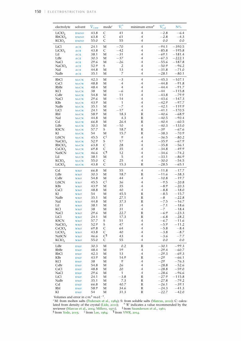
150 electrostriction data
electrolyte solvent V i intr mode* V−◦i minimum error† V
−◦i el N%
LiClO4 dmso 43.8 C 41 4 −2.8 −6.4RbClO4 dmso 63.8 C 61 4 −2.8 −4.3KClO4 dmso 55.0 C 55 4 0.0 0.0
LiCl ace 24.1 M −70 4 −94.1 −390.5LiClO4 ace 43.8 C −42 4 −85.8 −195.8LiI ace 38.1 M −31 4 −69.1 −181.4LiBr ace 30.3 M −37 4 −67.3 −222.1NaCl ace 29.6 M −26 4 −55.6 −187.8NaClO4 ace 52.9 S 2 4 −50.9 −96.2NaI ace 44.8 M 13 4 −31.8 −71.0NaBr ace 35.1 M 7 4 −28.1 −80.1
RbCl mecn 42.3 M −3 4 −45.3 −107.1CsCl mecn 48.8 M 4 4 −44.8 −91.8RbBr mecn 48.4 M 4 4 −44.4 −91.7KCl mecn 38 M −6 4 −44 −115.8CsBr mecn 54.8 M 11 4 −43.8 −79.9NaCl mecn 29.6 M −14 4 −43.6 −147.3KBr mecn 43.9 M 1 4 −42.9 −97.7NaBr mecn 35.1 M −7 4 −42.1 −119.9LiCl mecn 24.1 M −17 4 −41.1 −170.5RbI mecn 58.9 M 18.3 R −40.6 −68.9NaI mecn 44.8 M 4.3 R −40.5 −90.4CsI mecn 66.8 M 26.4 R −40.4 −60.5LiBr mecn 30.3 M −10 4 −40.3 −133.0KSCN mecn 57.7 S 18.7 R −39 −67.6KI mecn 54 M 15.7 R −38.3 −70.9LiSCN mecn 45.5 C‖ 9 4 −36.5 −80.2NaClO4 mecn 52.9 S 17 4 −35.9 −67.9RbClO4 mecn 63.8 C 28 4 −35.8 −56.1CsClO4 mecn 69.8 C 35 4 −34.8 −49.9NaSCN mecn 46.6 C¶ 12 4 −34.6 −74.2LiI mecn 38.1 M 5 4 −33.1 −86.9KClO4 mecn 55.0 C 25 4 −30.0 −54.5LiClO4 mecn 43.8 C 15.3 R −28.5 −65.1
CsI nmf 66.8 M 55 4 −11.8 −17.7LiBr nmf 30.3 M 18.7 R −11.6 −38.3CsBr nmf 54.8 M 44 4 −10.8 −19.7LiSCN nmf 45.5 C‖ 36 4 −9.5 −20.8KBr nmf 43.9 M 35 4 −8.9 −20.3CsCl nmf 48.8 M 40 4 −8.8 −18.0KI nmf 54 M 45.5 R −8.5 −15.7NaBr nmf 35.1 M 27.1 R −8 −22.8NaI nmf 44.8 M 37.3 R −7.5 −16.7LiI nmf 38.1 M 31 4 −7.1 −18.6KCl nmf 38 M 31 4 −7 −18.4NaCl nmf 29.6 M 22.7 R −6.9 −23.3LiCl nmf 24.1 M 17.3 R −6.8 −28.2KSCN nmf 57.7 S 51 4 −6.7 −11.6NaClO4 nmf 52.9 S 47 4 −5.9 −11.2CsClO4 nmf 69.8 C 64 4 −5.8 −8.4LiClO4 nmf 43.8 C 40 4 −3.8 −8.7NaSCN nmf 46.6 C¶ 43 4 −3.6 −7.7KClO4 nmf 55.0 C 55 4 0.0 0.0
LiBr dmf 30.3 M 0.2 R −30.1 −99.3RbBr dmf 48.4 M 19 4 −29.4 −60.7RbCl dmf 42.3 M 13 4 −29.3 −69.3KBr dmf 43.9 M 14.9 R −29 −66.1KCl dmf 38 M 9 4 −29 −76.3CsBr dmf 54.8 M 26 4 −28.8 −52.6CsCl dmf 48.8 M 20 4 −28.8 −59.0NaCl dmf 29.6 M 1 4 −28.6 −96.6LiCl dmf 24.1 M −3.8 R −27.9 −115.8NaBr dmf 35.1 M 7.3 R −27.8 −79.2CsI dmf 66.8 M 40.7 R −26.1 −39.1RbI dmf 58.9 M 34.6 R −24.3 −41.3KI dmf 54 M 31.3 R −22.7 −42.0
Volumes and error in cm3mol−1.* M: from molten salts (Pedersen et al., 1984); S: from soluble salts (Marcus, 2010); C: calcu-lated from density of the crystal (Lide, 2010); † ‘R’ indicates a value recommended by thereviewer (Marcus et al., 2004; Millero, 1971). ‡ from Saunderson et al., 1961;§ from Yode, 2015; ‖ from Lee, 1964; ¶ from VWR, 2014.

bibliography for the current appendix 151
electrolyte solvent V i intr mode* V−◦i minimum error† V
−◦i el N%
NaI dmf 44.8 M 22.2 R −22.6 −50.4LiI dmf 38.1 M 16 4 −22.1 −58.0NaClO4 dmf 52.9 S 33 4 −19.9 −37.6RbClO4 dmf 63.8 C 45 4 −18.8 −29.4CsClO4 dmf 69.8 C 52 4 −17.8 −25.5LiClO4 dmf 43.8 C 27 4 −16.8 −38.4KClO4 dmf 55.0 C 41 4 −14.0 −25.4
Volumes and error in cm3mol−1.* M: from molten salts (Pedersen et al., 1984); S: from soluble salts (Marcus, 2010); C: calcu-lated from density of the crystal (Lide, 2010); † ‘R’ indicates a value recommended by thereviewer (Marcus et al., 2004; Millero, 1971). ‡ from Saunderson et al., 1961;§ from Yode, 2015; ‖ from Lee, 1964; ¶ from VWR, 2014.
bibliography for the current appendixLee, D. A.
1964 ‘Anhydrous Lithium Thiocyanate’, Inorg. Chem. 3, 2, pp. 289–290, doi: 10.1021/ic50012a039.
Lide, D. R.2010 (ed.), CRC Handbook of Chemistry and Physics, 90th ed., CRC Press/Taylor
and Francis, Boca Raton, FL.
Marcus, Y.2010 ‘On the Intrinsic Volumes of Ions in Aqueous Solutions’, English, J. Solu-
tion Chem. 39, 7, pp. 1031–1038, doi: 10.1007/s10953-010-9553-6.
Marcus, Y. and G. T. Hefter2004 ‘Standard Partial Molar Volumes of Electrolytes and Ions in Nonaqueous
Solvents’, Chem. Rev. 104, pp. 3405–3452, doi: 10.1021/cr030047d.
Millero, F. J.1971 ‘The Molal Volumes of Electrolytes’, Chem. Rev. 71, 2, pp. 147–176, doi:
10.1021/cr60270a001.
Pedersen, T. G., C. Dethlefsen and A. Hvidt1984 ‘Volumetric Properties of Aqueous Solutions of Alkali Halides’, English,
Carlsberg Res. Commun. 49, 3, pp. 445–455, doi: 10.1007/BF02907785.
Saunderson, C. and R. B. Ferguson1961 ‘Crystal Data for Anhydrous Lithium Acetate’, Acta Crystallogr. 14, 3, p. 321.
VWR2014 Sodium Thiocyanate Density, ca.vwr.com/store/catalog/product.jsp?
catalog_number=CAAA33388-A3.
Yode, R.2015 ‘Cesium Acetate’, in Encyclopedia of Reagents for Organic Synthesis, John
Wiley & Sons, Ltd, isbn: 9780470842898, doi: 10.1002/047084289X.rn01845.
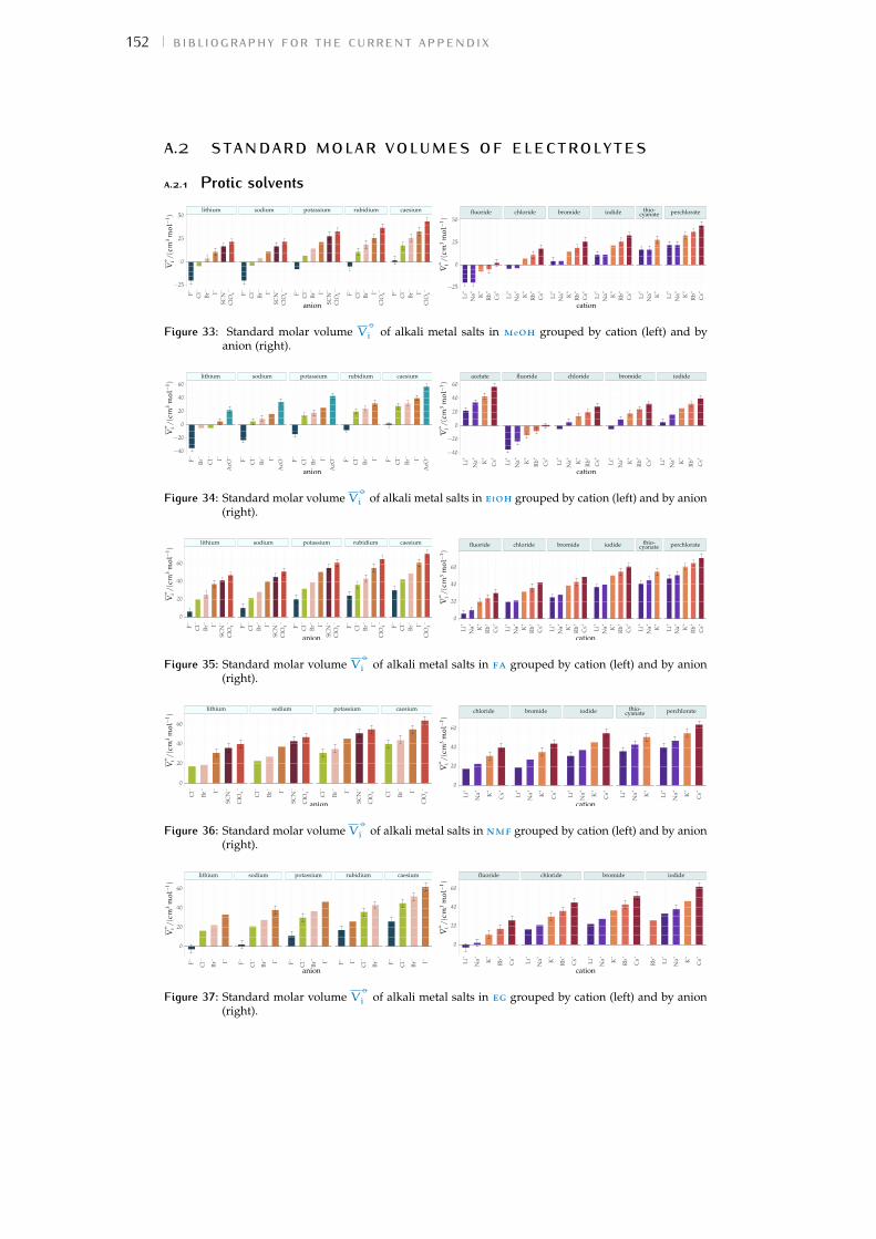
152 bibliography for the current appendix
a.2 standard molar volumes of electrolytesa.2.1 Protic solvents
lithium sodium potassium rubidium caesiumBr
–C
l–
ClO
4–
F– I–
SCN
–
Br–
Cl–
ClO
4–
F– I–
SCN
–
Br–
Cl–
ClO
4–
F– I–
SCN
–
Br–
Cl–
ClO
4–
F– I–
Br–
Cl–
ClO
4–
F– I–
−25
0
25
50
anion
V−◦ i/(cm
3mol−
1) fluoride chloride bromide iodide thio-
cyanate perchlorate
Cs+
K+
Li+
Na+
Rb+
Cs+
K+
Li+
Na+
Rb+
Cs+
K+
Li+
Na+
Rb+
Cs+
K+
Li+
Na+
Rb+
K+
Li+
Na+
Cs+
K+
Li+
Na+
Rb+
−25
0
25
50
cation
V−◦ i/(cm
3mol−
1)
Figure 33: Standard molar volume V−◦i of alkali metal salts in meoh grouped by cation (left) and by
anion (right).
lithium sodium potassium rubidium caesium
Br–
Cl–
F– I–
AcO
–
Br–
Cl–
F– I–
AcO
–
Br–
Cl–
F– I–
AcO
–
Br–
Cl–
F– I–
Br–
Cl–
F– I–
AcO
–
−40
−20
0
20
40
60
anion
V−◦ i/(cm
3mol−
1)
acetate fluoride chloride bromide iodide
Cs+
K+
Li+
Na+
Cs+
K+
Li+
Na+
Rb+
Cs+
K+
Li+
Na+
Rb+
Cs+
K+
Li+
Na+
Rb+
Cs+
K+
Li+
Na+
Rb+
−40
−20
0
20
40
60
cation
V−◦ i/(cm
3mol−
1)
Figure 34: Standard molar volume V−◦i of alkali metal salts in etoh grouped by cation (left) and by anion
(right).
lithium sodium potassium rubidium caesium
Br–
Cl–
ClO
4–
F– I–
SCN
–
Br–
Cl–
ClO
4–
F– I–
SCN
–
Br–
Cl–
ClO
4–
F– I–
SCN
–
Br–
Cl–
ClO
4–
F– I–
Br–
Cl–
ClO
4–
F– I–
0
20
40
60
anion
V−◦ i/(cm
3mol−
1) fluoride chloride bromide iodide thio-
cyanate perchlorate
Cs+
K+
Li+
Na+
Rb+
Cs+
K+
Li+
Na+
Rb+
Cs+
K+
Li+
Na+
Rb+
Cs+
K+
Li+
Na+
Rb+
K+
Li+
Na+
Cs+
K+
Li+
Na+
Rb+
0
20
40
60
cation
V−◦ i/(cm
3mol−
1)
Figure 35: Standard molar volume V−◦i of alkali metal salts in fa grouped by cation (left) and by anion
(right).
lithium sodium potassium caesium
Br–
Cl–
ClO
4–I–
SCN
–
Br–
Cl–
ClO
4–I–
SCN
–
Br–
Cl–
ClO
4–I–
SCN
–
Br–
Cl–
ClO
4–I–
0
20
40
60
anion
V−◦ i/(cm
3mol−
1) chloride bromide iodide thio-
cyanate perchlorate
Cs+
K+
Li+
Na+
Cs+
K+
Li+
Na+
Cs+
K+
Li+
Na+
K+
Li+
Na+
Cs+
K+
Li+
Na+
0
20
40
60
cation
V−◦ i/(cm
3mol−
1)
Figure 36: Standard molar volume V−◦i of alkali metal salts in nmf grouped by cation (left) and by anion
(right).
lithium sodium potassium rubidium caesium
Br–
Cl–
F– I–
Br–
Cl–
F– I–
Br–
Cl–
F– I–
Br–
Cl–
F– I–
Br–
Cl–
F– I–
0
20
40
60
anion
V−◦ i/(cm
3mol−
1)
fluoride chloride bromide iodide
Cs+
K+
Li+
Na+
Rb+
Cs+
K+
Li+
Na+
Rb+
Cs+
K+
Li+
Na+
Rb+
Cs+
K+
Li+
Na+
Rb+
0
20
40
60
cation
V−◦ i/(cm
3mol−
1)
Figure 37: Standard molar volume V−◦i of alkali metal salts in eg grouped by cation (left) and by anion
(right).

a.2 standard molar volumes of electrolytes 153
a.2.2 Aprotic solventslithium sodium potassium rubidium caesium
Br–
Cl–
ClO
4–I–
Br–
Cl–
ClO
4–I–
Br–
Cl–
ClO
4–I–
Br–
Cl–
ClO
4–I–
Br–
Cl–
ClO
4–I–
0
20
40
60
anion
V−◦ i/(cm
3mol−
1)
chloride bromide iodide perchlorate
Cs+
K+
Li+
Na+
Rb+
Cs+
K+
Li+
Na+
Rb+
Cs+
K+
Li+
Na+
Rb+
Cs+
K+
Li+
Na+
Rb+
0
20
40
60
cation
V−◦ i/(cm
3mol−
1)
Figure 38: Standard molar volume V−◦i of alkali metal salts in pc grouped by cation (left) and by anion
(right).
lithium sodium potassium
ClO
4–I–
ClO
4–I–
ClO
4–I–
0
20
40
60
anion
V−◦ i/(cm
3mol−
1)
iodide perchlorate
K+
Li+
Na+
K+
Li+
Na+
0
20
40
60
cation
V−◦ i/(cm
3mol−
1)
Figure 39: Standard molar volume V−◦i of alkali metal salts in ec grouped by cation (left) and by anion
(right).
lithium sodium potassium rubidium caesium
Br–
Cl–
ClO
4–
F– I–
Br–
Cl–
ClO
4–
F– I–
Br–
Cl–
ClO
4–
F– I–
Br–
Cl–
ClO
4–
F– I–
Br–
Cl–
ClO
4–
F– I–
0
20
40
60
anion
V−◦ i/(cm
3mol−
1)
fluoride chloride bromide iodide perchlorate
Cs+
K+
Li+
Na+
Rb+
Cs+
K+
Li+
Na+
Rb+
Cs+
K+
Li+
Na+
Rb+
Cs+
K+
Li+
Na+
Rb+
Cs+
K+
Li+
Na+
Rb+
0
20
40
60
cation
V−◦ i/(cm
3mol−
1)
Figure 40: Standard molar volume V−◦i of alkali metal salts in dmso grouped by cation (left) and by
anion (right).
lithium sodium
Br–
Cl–
ClO
4– I–
Br–
Cl–
ClO
4– I–
−75
−50
−25
0
anion
V−◦ i/(cm
3mol−
1)
chloride bromide iodide perchlorate
Li+
Na+
Li+
Na+
Li+
Na+
Li+
Na+
−75
−50
−25
0
cation
V−◦ i/(cm
3mol−
1)
Figure 41: Standard molar volume V−◦i of alkali metal salts in ace grouped by cation (left) and by anion
(right).
lithium sodium potassium rubidium caesium
Br–
Cl–
ClO
4–I–
SCN
–
Br–
Cl–
ClO
4–I–
SCN
–
Br–
Cl–
ClO
4–I–
SCN
–
Br–
Cl–
ClO
4–I–
Br–
Cl–
ClO
4–I–
−20
0
20
40
anion
V−◦ i/(cm
3mol−
1) chloride bromide iodide thio-
cyanate perchlorate
Cs+
K+
Li+
Na+
Rb+
Cs+
K+
Li+
Na+
Rb+
Cs+
K+
Li+
Na+
Rb+
K+
Li+
Na+
Cs+
K+
Li+
Na+
Rb+
−20
0
20
40
cation
V−◦ i/(cm
3mol−
1)
Figure 42: Standard molar volume V−◦i of alkali metal salts in mecn grouped by cation (left) and by
anion (right).
lithium sodium potassium rubidium caesium
Br–
Cl–
ClO
4–I–
Br–
Cl–
ClO
4–I–
Br–
Cl–
ClO
4–I–
Br–
Cl–
ClO
4–I–
Br–
Cl–
ClO
4–I–
0
20
40
anion
V−◦ i/(cm
3mol−
1)
chloride bromide iodide perchlorate
Cs+
K+
Li+
Na+
Rb+
Cs+
K+
Li+
Na+
Rb+
Cs+
K+
Li+
Na+
Rb+
Cs+
K+
Li+
Na+
Rb+
0
20
40
cation
V−◦ i/(cm
3mol−
1)
Figure 43: Standard molar volume V−◦i of alkali metal salts in dmf grouped by cation (left) and by anion
(right).

154 bibliography for the current appendix
a.3 electrostrictive volume of electrolytesThe labels above the bars in each plot indicate the method of estimation of the intrinsic molar volumeused in the calculations. M: extrapolation from molten salts, from Pedersen et al. (1984); S: from ‘solublesalts’ (Marcus, 2010); C: crystal volume, as in Eq. [5].
a.3.1 Protic solvents
MM CM MC MM SM M C MM CMM M MM CC M MM CMM
lithium sodium potassium rubidium caesiumBr
–
Cl–
ClO
4–
F– I–
SCN
–
Br–
Cl–
ClO
4–
F– I–
SCN
–
Br–
Cl–
ClO
4–
F–I–
SCN
–
Br–
Cl–
ClO
4–
F– I–
Br–
Cl–
ClO
4–
F–I–
−40
−30
−20
−10
0
anion
V−◦ ie
l/(cm
3mol−
1)
M MMMC MM MM M MM MM M M M MM M M CC C C CS C
fluoride chloride bromide iodide thio-cyanate perchlorate
Cs+
K+
Li+
Na+
Rb+
Cs+
K+
Li+
Na+
Rb+
Cs+
K+
Li+
Na+
Rb+
Cs+
K+
Li+
Na+
Rb+
K+
Li+
Na+
Cs+
K+
Li+
Na+
Rb+
−40
−30
−20
−10
0
cation
V−◦ ie
l/(cm
3mol−
1)
Figure 44: Standard molar electrostrictive volume V−◦i el of alkali metal salts in meoh grouped by cation
(left) and by anion (right).
M MM M C M MM M M M MM M M M MC M M MM M C
lithium sodium potassium rubidium caesium
Br–
Cl–
F– I–
AcO
–
Br–
Cl–
F– I–
AcO
–
Br–
Cl–
F– I–
AcO
–
Br–
Cl–
F– I–
Br–
Cl–
F– I–
AcO
–
−50
−40
−30
−20
−10
0
anion
V−◦ ie
l/(cm
3mol−
1) C MC M MMM MC MMM M M MMM M M MMM M M
acetate fluoride chloride bromide iodide
Cs+
K+
Li+
Na+
Cs+
K+
Li+
Na+
Rb+
Cs+
K+
Li+
Na+
Rb+
Cs+
K+
Li+
Na+
Rb+
Cs+
K+
Li+
Na+
Rb+
−50
−40
−30
−20
−10
0
cation
V−◦ ie
l/(cm
3mol−
1)
Figure 45: Standard molar electrostrictive volume V−◦i el of alkali metal salts in etoh grouped by cation
(left) and by anion (right).
M M CM MC MM SM M C MM CM M M MM CC M MM CMM
lithium sodium potassium rubidium caesium
Br–
Cl–
ClO
4–
F– I–
SCN
–
Br–
Cl–
ClO
4–
F– I–
SCN
–
Br–
Cl–
ClO
4–
F– I–
SCN
–
Br–
Cl–
ClO
4–
F– I–
Br–
Cl–
ClO
4–
F–I–
−10
−5
0
5
10
anion
V−◦ ie
l/(cm
3mol−
1)
MMMMC M M MM M M MMM M M M MM M MC C C CCS C
fluoride chloride bromide iodide thio-cyanate perchlorate
Cs+
K+
Li+
Na+
Rb+
Cs+
K+
Li+
Na+
Rb+
Cs+
K+
Li+
Na+
Rb+
Cs+
K+
Li+
Na+
Rb+
K+
Li+
Na+
Cs+
K+
Li+
Na+
Rb+
−10
−5
0
5
10
cation
V−◦ ie
l/(cm
3mol−
1)
Figure 46: Standard molar electrostrictive volume V−◦i el of alkali metal salts in fa grouped by cation (left)
and by anion (right).
M M CMC M M SM C M M CM M M M CM
lithium sodium potassium caesium
Br–
Cl–
ClO
4–I–
SCN
–
Br–
Cl–
ClO
4–I–
SCN
–
Br–
Cl–
ClO
4–I–
SCN
–
Br–
Cl–
ClO
4–I–
−15
−10
−5
0
5
anion
V−◦ ie
l/(cm
3mol−
1)
M M MM M MM M M M MM MC C C CCS
chloride bromide iodide thio-cyanate perchlorate
Cs+
K+
Li+
Na+
Cs+
K+
Li+
Na+
Cs+
K+
Li+
Na+
K+
Li+
Na+
Cs+
K+
Li+
Na+
−15
−10
−5
0
5
cation
V−◦ ie
l/(cm
3mol−
1)
Figure 47: Standard molar electrostrictive volume V−◦i el of alkali metal salts in nmf grouped by cation
(left) and by anion (right).
M MM M MMM M MMM M MMCM MMM M
lithium sodium potassium rubidium caesium
Br–
Cl–
F– I–
Br–
Cl–
F– I–
Br–
Cl–
F– I–
Br–
Cl–
F–I–
Br–
Cl–
F– I–
−30
−20
−10
0
anion
V−◦ ie
l/(cm
3mol−
1) MMM MC MM MM M MMM M M MM MMM
fluoride chloride bromide iodide
Cs+
K+
Li+
Na+
Rb+
Cs+
K+
Li+
Na+
Rb+
Cs+
K+
Li+
Na+
Rb+
Cs+
K+
Li+
Na+
Rb+
−30
−20
−10
0
cation
V−◦ ie
l/(cm
3mol−
1)
Figure 48: Standard molar electrostrictive volume V−◦i el of alkali metal salts in eg grouped by cation (left)
and by anion (right).
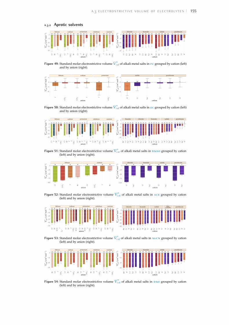
a.3 electrostrictive volume of electrolytes 155
a.3.2 Aprotic solvents
MM CM MM SM MM CM MM CM MM CM
lithium sodium potassium rubidium caesium
Br–
Cl–
ClO
4–I–
Br–
Cl–
ClO
4–I–
Br–
Cl–
ClO
4–I–
Br–
Cl–
ClO
4–I–
Br–
Cl–
ClO
4–I–
−20
−15
−10
−5
0
anion
V−◦ ie
l/(cm
3mol−
1) M MM M M M MM MM M M M MM C CCS C
chloride bromide iodide perchlorate
Cs+
K+
Li+
Na+
Rb+
Cs+
K+
Li+
Na+
Rb+
Cs+
K+
Li+
Na+
Rb+
Cs+
K+
Li+
Na+
Rb+
−20
−15
−10
−5
0
cation
V−◦ ie
l/(cm
3mol−
1)
Figure 49: Standard molar electrostrictive volume V−◦i el of alkali metal salts in pc grouped by cation (left)
and by anion (right).
CM S M CM
lithium sodium potassium
ClO
4–I–
ClO
4– I–
ClO
4–I–
−8
−4
0
4
anion
V−◦ ie
l/(cm
3mol−
1)
M M M CCS
iodide perchlorate
K+
Li+
Na+
K+
Li+
Na+
−8
−4
0
4
cation
V−◦ ie
l/(cm
3mol−
1)
Figure 50: Standard molar electrostrictive volume V−◦i el of alkali metal salts in ec grouped by cation (left)
and by anion (right).
MM CM M MM SM M MM CM M MM CC M MM CM M
lithium sodium potassium rubidium caesium
Br–
Cl–
ClO
4–
F– I–
Br–
Cl–
ClO
4–
F– I–
Br–
Cl–
ClO
4–
F– I–
Br–
Cl–
ClO
4–
F– I–
Br–
Cl–
ClO
4–
F– I–
−20
−15
−10
−5
0
5
anion
V−◦ ie
l/(cm
3mol−
1)
MMM MC MMM M M MMM M M M M M M M C CCS C
fluoride chloride bromide iodide perchlorate
Cs+
K+
Li+
Na+
Rb+
Cs+
K+
Li+
Na+
Rb+
Cs+
K+
Li+
Na+
Rb+
Cs+
K+
Li+
Na+
Rb+
Cs+
K+
Li+
Na+
Rb+
−20
−15
−10
−5
0
5
cation
V−◦ ie
l/(cm
3mol−
1)
Figure 51: Standard molar electrostrictive volume V−◦i el of alkali metal salts in dmso grouped by cation
(left) and by anion (right).
MM C M MM S M
lithium sodium
Br–
Cl–
ClO
4– I–
Br–
Cl–
ClO
4– I–
−100
−75
−50
−25
0
anion
V−◦ ie
l/(cm
3mol−
1) M M M M M M C S
chloride bromide iodide perchlorate
Li+
Na+
Li+
Na+
Li+
Na+
Li+
Na+
−100
−75
−50
−25
0
cation
V−◦ ie
l/(cm
3mol−
1)
Figure 52: Standard molar electrostrictive volume V−◦i el of alkali metal salts in ace grouped by cation
(left) and by anion (right).
MM CMC MM SM C MM CMM MM CM MM CM
lithium sodium potassium rubidium caesium
Br–
Cl–
Cs+
I–
SCN
–
Br–
Cl–
ClO
4–I–
SCN
–
Br–
Cl–
ClO
4–I–
SCN
–
Br–
Cl–
ClO
4–I–
Br–
Cl–
ClO
4–I–
−50
−40
−30
−20
−10
0
anion
V−◦ ie
l/(cm
3mol−
1)
M M MMM M M MMM M M MMM M C C C C CS C
chloride bromide iodide thio-cyanate perchlorate
Cs+
K+
Li+
Na+
Rb+
Cs+
K+
Li+
Na+
Rb+
Cs+
K+
Li+
Na+
Rb+
K+
Li+
Na+
Cs+
K+
Li+
Na+
Rb+
−50
−40
−30
−20
−10
0
cation
V−◦ ie
l/(cm
3mol−
1)
Figure 53: Standard molar electrostrictive volume V−◦i el of alkali metal salts in mecn grouped by cation
(left) and by anion (right).
M M CM MM SM M M CM M M CM M M CM
lithium sodium potassium rubidium caesium
Br–
Cl–
ClO
4–I–
Br–
Cl–
ClO
4–I–
Br–
Cl–
ClO
4–I–
Br–
Cl–
ClO
4–I–
Br–
Cl–
ClO
4–I–
−30
−20
−10
0
anion
V−◦ ie
l/(cm
3mol−
1) MM MMM MMM MM M M MMM C CCS C
chloride bromide iodide perchlorate
Cs+
K+
Li+
Na+
Rb+
Cs+
K+
Li+
Na+
Rb+
Cs+
K+
Li+
Na+
Rb+
Cs+
K+
Li+
Na+
Rb+
−30
−20
−10
0
cation
V−◦ ie
l/(cm
3mol−
1)
Figure 54: Standard molar electrostrictive volume V−◦i el of alkali metal salts in dmf grouped by cation
(left) and by anion (right).

156 bibliography for the current appendix
a.4 normalised electrostrictive volumesThe labels above the bars in each plot indicate the method of estimation of the intrinsic molar volumeused in the calculations. M: extrapolation from molten salts, from Pedersen et al. (1984); S: from ‘solublesalts’ (Marcus, 2010); C: crystal volume, as in Eq. [5].
a.4.1 Protic solvents
MM CM M C MM SM M C MM CM M M MM CC M MM CM M
lithium sodium potassium rubidium caesium
Br–
Cl–
ClO
4–
F– I–
SCN
–
Br–
Cl–
ClO
4–
F– I–
SCN
–
Br–
Cl–
ClO
4–
F– I–
SCN
–
Br–
Cl–
ClO
4–
F– I–
Br–
Cl–
ClO
4–
F– I–
−200
−100
0
anion
N%MMM M C MMM M M MMMM M MMMM M MCC CCCS C
fluoride chloride bromide iodide thio-cyanate perchlorate
Cs+
K+
Li+
Na+
Rb+
Cs+
K+
Li+
Na+
Rb+
Cs+
K+
Li+
Na+
Rb+
Cs+
K+
Li+
Na+
Rb+
K+
Li+
Na+
Cs+
K+
Li+
Na+
Rb+
−200
−100
0
cation
N%
Figure 55: Normalised standard molar electrostrictive volumeN% of alkali metal salts in meoh groupedby cation (left) and by anion (right).
MMM M C MMM M M MMM M M MMC M MMM M C
lithium sodium potassium rubidium caesium
Br–
Cl–
F– I–
AcO
–
Br–
Cl–
F– I–
AcO
–
Br–
Cl–
F– I–
AcO
–
Br–
Cl–
F– I–
Br–
Cl–
F– I–
AcO
–
−400
−300
−200
−100
0
anion
N% CMC M MMM M C MMM M M MMM M M MMM M M
acetate fluoride chloride bromide iodide
Cs+
K+
Li+
Na+
Cs+
K+
Li+
Na+
Rb+
Cs+
K+
Li+
Na+
Rb+
Cs+
K+
Li+
Na+
Rb+
Cs+
K+
Li+
Na+
Rb+
−400
−300
−200
−100
0
cation
N%
Figure 56: Normalised standard molar electrostrictive volumeN% of alkali metal salts in etoh groupedby cation (left) and by anion (right).
M M CM MC MM SM M C MM CM M M MM CC M MM CM M
lithium sodium potassium rubidium caesium
Br–
Cl–
ClO
4–
F– I–
SCN
–
Br–
Cl–
ClO
4–
F– I–
SCN
–
Br–
Cl–
ClO
4–
F– I–
SCN
–
Br–
Cl–
ClO
4–
F– I–
Br–
Cl–
ClO
4–
F– I–
−50
−40
−30
−20
−10
0
10
anion
N%
MMM M C MMMM M MMMM M M M MM M MC C C CCS C
fluoride chloride bromide iodide thio-cyanate perchlorate
Cs+
K+
Li+
Na+
Rb+
Cs+
K+
Li+
Na+
Rb+
Cs+
K+
Li+
Na+
Rb+
Cs+
K+
Li+
Na+
Rb+
K+
Li+
Na+
Cs+
K+
Li+
Na+
Rb+
−50
−40
−30
−20
−10
0
10
cation
N%
Figure 57: Normalised standard molar electrostrictive volume N% of alkali metal salts in fa groupedby cation (left) and by anion (right).
M M CMC MM SM C M M CM M M M CM
lithium sodium potassium caesium
Br–
Cl–
ClO
4–I–
SCN
–
Br–
Cl–
ClO
4–I–
SCN
–
Br–
Cl–
ClO
4–I–
SCN
–
Br–
Cl–
ClO
4–I–
−40
−30
−20
−10
0
anion
N%MMM M MMM M M MM M MC C C CCS
chloride bromide iodide thio-cyanate perchlorate
Cs+
K+
Li+
Na+
Cs+
K+
Li+
Na+
Cs+
K+
Li+
Na+
K+
Li+
Na+
Cs+
K+
Li+
Na+
−40
−30
−20
−10
0
cation
N%
Figure 58: Normalised standard molar electrostrictive volumeN% of alkali metal salts in nmf groupedby cation (left) and by anion (right).
MMM M MMM M MMM M MMCM MMM M
lithium sodium potassium rubidium caesium
Br–
Cl–
F– I–
Br–
Cl–
F– I–
Br–
Cl–
F– I–
Br–
Cl–
F–I–
Br–
Cl–
F– I–
−100
−50
0
anion
N% MMM M C MMM M M MMM M M MM MMM
fluoride chloride bromide iodide
Cs+
K+
Li+
Na+
Rb+
Cs+
K+
Li+
Na+
Rb+
Cs+
K+
Li+
Na+
Rb+
Cs+
K+
Li+
Na+
Rb+
−100
−50
0
cation
N%
Figure 59: Normalised standard molar electrostrictive volume N% of alkali metal salts in eg groupedby cation (left) and by anion (right).
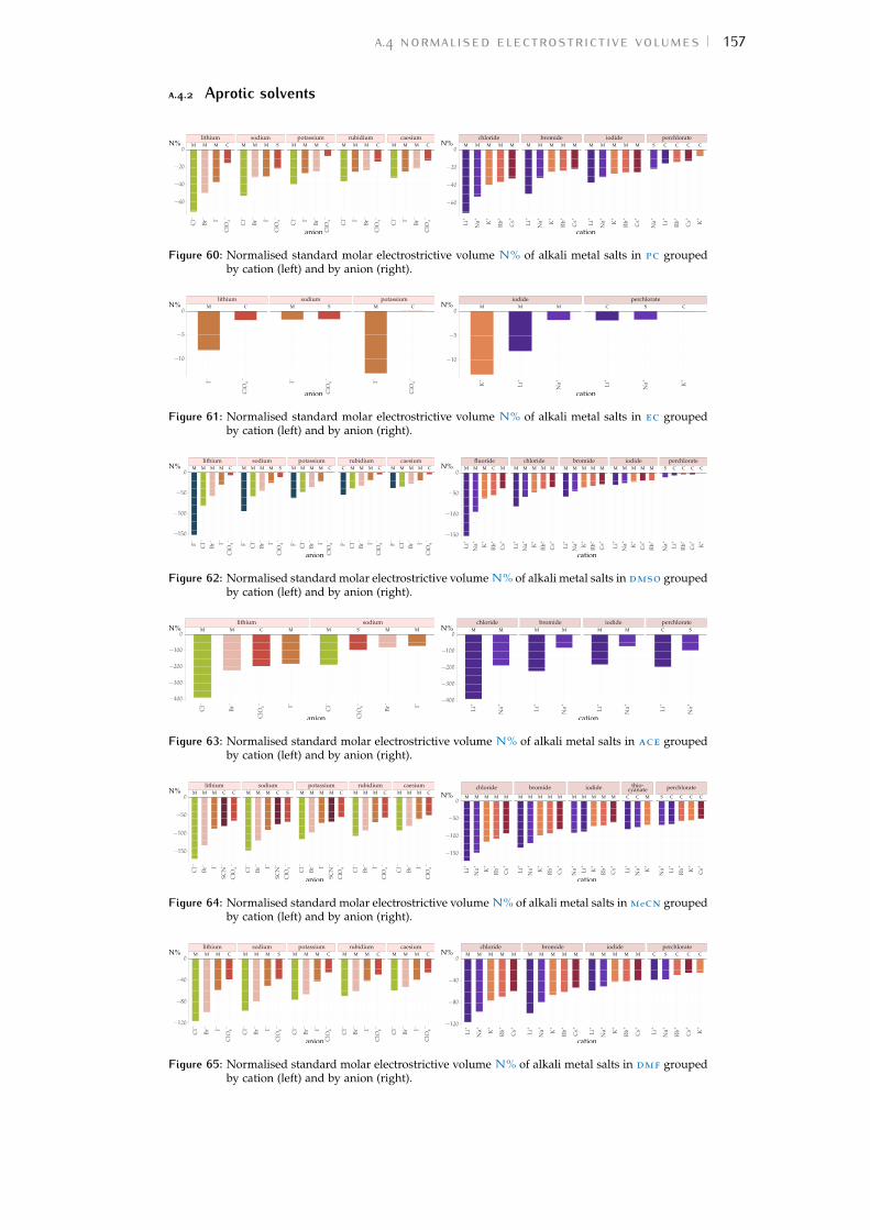
a.4 normalised electrostrictive volumes 157
a.4.2 Aprotic solvents
MM CM MM SM MM CM MM CM MM CM
lithium sodium potassium rubidium caesium
Br–
Cl–
ClO
4–I–
Br–
Cl–
ClO
4–I–
Br–
Cl–
ClO
4–I–
Br–
Cl–
ClO
4–I–
Br–
Cl–
ClO
4–I–
−60
−40
−20
0
anion
N% MMM M M MMM M M MMM M M C CCS C
chloride bromide iodide perchlorate
Cs+
K+
Li+
Na+
Rb+
Cs+
K+
Li+
Na+
Rb+
Cs+
K+
Li+
Na+
Rb+
Cs+
K+
Li+
Na+
Rb+
−60
−40
−20
0
cation
N%
Figure 60: Normalised standard molar electrostrictive volume N% of alkali metal salts in pc groupedby cation (left) and by anion (right).
CM SM CM
lithium sodium potassium
ClO
4–I–
ClO
4–I–
ClO
4–I–
−10
−5
0
anion
N% M M M CC S
iodide perchlorate
K+
Li+
Na+
K+
Li+
Na+
−10
−5
0
cation
N%
Figure 61: Normalised standard molar electrostrictive volume N% of alkali metal salts in ec groupedby cation (left) and by anion (right).
MM CM M MM SM M MM CM M MM CC M MM CM M
lithium sodium potassium rubidium caesium
Br–
Cl–
ClO
4–
F– I–
Br–
Cl–
ClO
4–
F– I–
Br–
Cl–
ClO
4–
F– I–
Br–
Cl–
ClO
4–
F– I–
Br–
Cl–
ClO
4–
F– I–
−150
−100
−50
0
anion
N% MMM M C MMM M M MMM M M MMM M M C CCS C
fluoride chloride bromide iodide perchlorate
Cs+
K+
Li+
Na+
Rb+
Cs+
K+
Li+
Na+
Rb+
Cs+
K+
Li+
Na+
Rb+
Cs+
K+
Li+
Na+
Rb+
Cs+
K+
Li+
Na+
Rb+
−150
−100
−50
0
cation
N%
Figure 62: Normalised standard molar electrostrictive volumeN% of alkali metal salts in dmso groupedby cation (left) and by anion (right).
MM C M MM S M
lithium sodium
Br–
Cl–
ClO
4– I–
Br–
Cl–
ClO
4– I–
−400
−300
−200
−100
0
anion
N% M M M M M M C S
chloride bromide iodide perchlorate
Li+
Na+
Li+
Na+
Li+
Na+
Li+
Na+
−400
−300
−200
−100
0
cation
N%
Figure 63: Normalised standard molar electrostrictive volume N% of alkali metal salts in ace groupedby cation (left) and by anion (right).
MM CM C MM SM C MM CM M MM CM MM CM
lithium sodium potassium rubidium caesium
Br–
Cl–
ClO
4–I–
SCN
–
Br–
Cl–
ClO
4–I–
SCN
–
Br–
Cl–
ClO
4–I–
SCN
–
Br–
Cl–
ClO
4–I–
Br–
Cl–
ClO
4–I–
−150
−100
−50
0
anion
N%MMM M M MMM M M MMMM M MC C CCCS C
chloride bromide iodide thio-cyanate perchlorate
Cs+
K+
Li+
Na+
Rb+
Cs+
K+
Li+
Na+
Rb+
Cs+
K+
Li+
Na+
Rb+
K+
Li+
Na+
Cs+
K+
Li+
Na+
Rb+
−150
−100
−50
0
cation
N%
Figure 64: Normalised standard molar electrostrictive volumeN% of alkali metal salts in mecn groupedby cation (left) and by anion (right).
MM CM MM SM MM CM MM CM MM CM
lithium sodium potassium rubidium caesium
Br–
Cl–
ClO
4–I–
Br–
Cl–
ClO
4–I–
Br–
Cl–
ClO
4–I–
Br–
Cl–
ClO
4–I–
Br–
Cl–
ClO
4–I–
−120
−80
−40
0
anion
N% MMM M M MMM M M MMM M M C CC S C
chloride bromide iodide perchlorate
Cs+
K+
Li+
Na+
Rb+
Cs+
K+
Li+
Na+
Rb+
Cs+
K+
Li+
Na+
Rb+
Cs+
K+
Li+
Na+
Rb+
−120
−80
−40
0
cation
N%
Figure 65: Normalised standard molar electrostrictive volumeN% of alkali metal salts in dmf groupedby cation (left) and by anion (right).

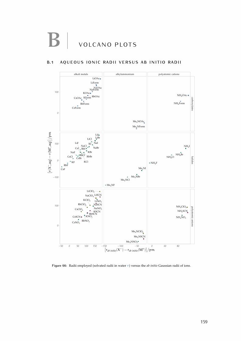
B V O LC A N O P LOT S
b.1 aqueous ionic radii versus ab initio radii
CsForm
KForm
LiForm
NaForm
RbForm
CsOAc
KOAc
LiOAc
NaOAc
RbOAc
CsBr
KBr
LiBr
NaBr
RbBrCsCl
KCl
LiCl
NaCl
RbCl
CsF
KF
LiF
NaF
RbF
CsI
KI
LiI
NaI
RbI
CsClO4
KClO4
LiClO4
NaClO4
RbClO4
CsNO3
KNO3
LiNO3
NaNO3
RbNO3
CsSCN
KSCN
LiSCN
NaSCN
RbSCN
Me4NForm
Me4NOAc
Me4NBrMe4NCl
Me4NF
Me4NI
Me4NClO4
Me4NNO3
Me4NSCN
NH4Form
NH4OAc
NH4BrNH4Cl
NH4F
NH4I
NH4ClO4
NH4NO3
NH4SCN
alkali metals alkylammonium polyatomic cations
carboxylateshalides
polyatomic
anions
−50 0 50 100 150 −150 −100 −50 0 40 80
0
100
−100
0
100
0
100
[rab initio(X– ) − rab initio(M+)
]/pm
[ r(X
– ,aq)
−r(
M+ ,a
q)]/pm
Figure 66: Radii employed (solvated radii in water r) versus the ab initio Gaussian radii of ions.
159
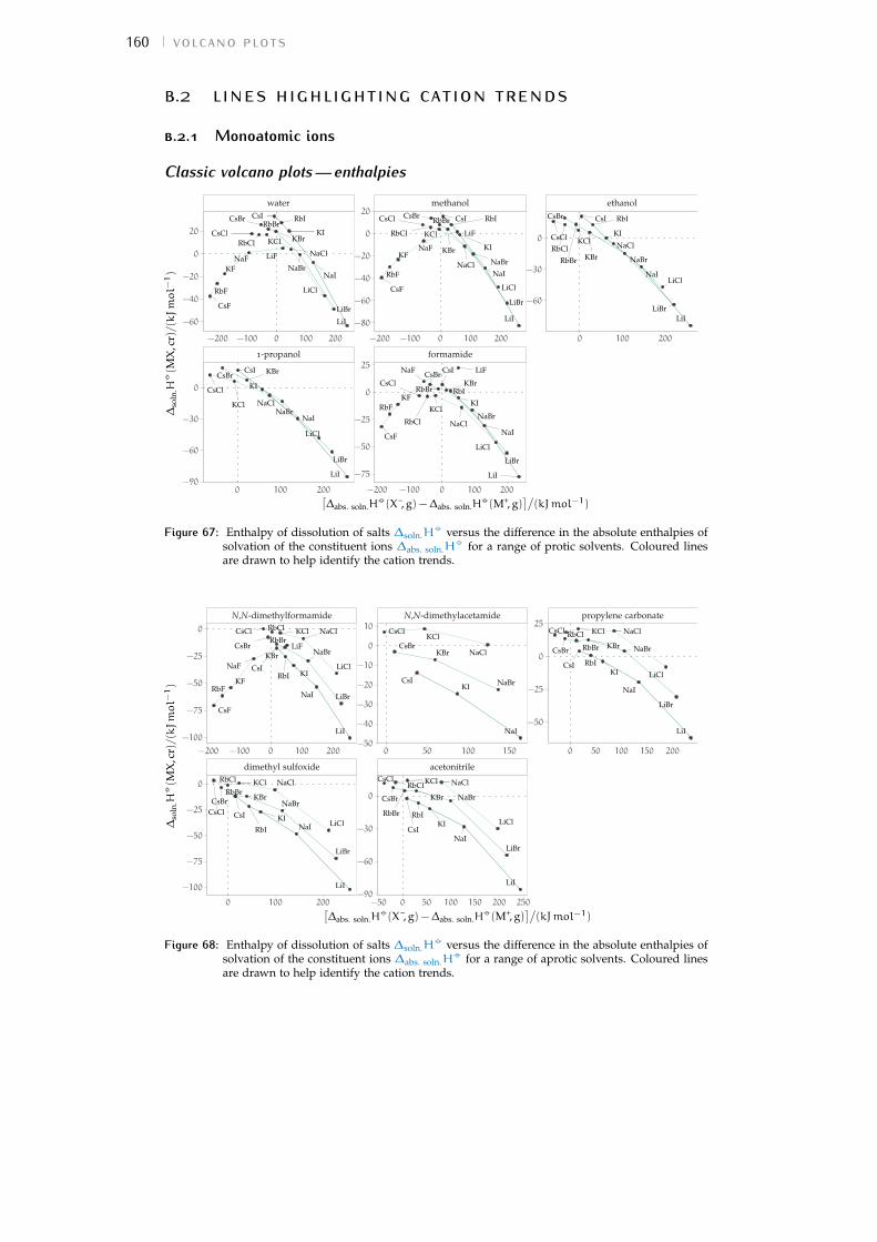
160 volcano plots
b.2 lines highlighting cation trendsb.2.1 Monoatomic ions
Classic volcano plots — enthalpies
NaBr
NaCl
NaI
CsF
RbBr
LiBr
LiF
RbF
KIKCl
KF
CsClKBr
NaF
LiI
CsI RbICsBr
LiCl
RbCl
KCl
CsI
CsCl
NaI
NaCl
KBr
LiCl
CsBr
NaBr
KI
LiI
LiBr
CsBr
RbCl
CsI
KIKBr
NaCl
LiCl
NaI
KCl
LiI
LiF
NaBr
LiBr
RbBr
RbF
KF
CsF
RbI
NaF
CsCl
LiCl
RbBr
NaBr
NaI
NaF
CsF
LiBr
RbI
RbF
LiF
RbCl
KI
LiI
CsICsBr
KF
NaCl
KBrCsCl
KCl
RbI
RbBr
CsI
KBr NaBr
KCl
CsBr
LiBr
KI
LiI
NaI
CsClNaClRbCl
LiCl
1-propanol formamide
water methanol ethanol
0 100 200 −200 −100 0 100 200
−200 −100 0 100 200 −200 −100 0 100 200 0 100 200
−60
−30
0
−80
−60
−40
−20
0
20
−75
−50
−25
0
25
−60
−40
−20
0
20
−90
−60
−30
0
[∆abs. soln.H
−◦ (X–, g) −∆abs. soln.H−◦ (M+, g)
]/(kJmol−1)
∆so
ln.H
−◦(M
X,c
r)/(kJmol−
1)
Figure 67: Enthalpy of dissolution of salts ∆soln.H−◦ versus the difference in the absolute enthalpies of
solvation of the constituent ions ∆abs. soln.H−◦ for a range of protic solvents. Coloured lines
are drawn to help identify the cation trends.
KFRbF
CsCl
CsF
KI
NaI
LiClRbI
LiF
CsI
KBrNaF
RbCl KCl
CsBr
NaCl
LiBr
RbBr
LiI
NaBr
RbI
CsCl
LiI
LiBr
CsILiCl
NaClKCl
KBrRbBr
NaI
RbCl
CsBr NaBr
KI
NaCl
NaI
CsBr
CsIKI
CsCl
KBr
KCl
NaBr
KCl
KBr
CsCl
CsI
NaBr
KI LiCl
LiBr
NaCl
RbI
NaI
LiI
RbBr
RbCl
CsBr
RbI
NaCl
LiBr
CsBr
KI
CsCl
NaI
NaBr
LiI
KBrRbBr
KCl
CsILiCl
RbCl
dimethyl sulfoxide acetonitrile
N,N-dimethylformamide N,N-dimethylacetamide propylene carbonate
0 100 200 −50 0 50 100 150 200 250
−200 −100 0 100 200 0 50 100 150 0 50 100 150 200
−50
−25
0
25
−50
−40
−30
−20
−10
0
10
−90
−60
−30
0
−100
−75
−50
−25
0
−100
−75
−50
−25
0
[∆abs. soln.H
−◦ (X–, g) −∆abs. soln.H−◦ (M+, g)
]/(kJmol−1)
∆so
ln.H
−◦(M
X,c
r)/(kJmol−
1)
Figure 68: Enthalpy of dissolution of salts ∆soln.H−◦ versus the difference in the absolute enthalpies of
solvation of the constituent ions ∆abs. soln.H−◦ for a range of aprotic solvents. Coloured lines
are drawn to help identify the cation trends.

b.2 lines highlighting cation trends 161
Classic volcano plots — enthalpies by cation
LiBr
LiF
LiI
LiCl
NaBrNaCl
NaINaF
KIKCl
KF
KBr
RbBr
RbF
RbIRbCl
CsI
CsClCsI
CsBr
LiCl
LiI
LiF
LiBr
NaCl
NaI
NaBrNaF
KI
KBrKCl
KF
RbCl
RbBr
RbF
RbI
CsBr CsI
CsI
CsCl
LiBrLiI
LiCl
NaBr
NaI
NaCl
KBr
KCl
KI
RbIRbBr
RbCl
CsICsBr
CsCl
LiCl
LiILiBr
NaI
NaClNaBr
KCl
KBr
KI
CsICsCl
CsBr
LiCl
LiBr
LiF
LiI
NaBr
NaI
NaFNaCl
KIKF
KBr
KCl
RbBr
RbIRbF
RbCl
CsI
CsICsBr
CsCl
water methanol ethanol 1-propanol formamideLi +
Na
+K
+R
b+
Cs +
−200−100 0 100 200 −200−100 0 100 200 −200−100 0 100 200 −200−100 0 100 200 −200−100 0 100 200
−50
0
−50
0
−50
0
−50
0
−50
0
[∆abs. soln.H
−◦ (X–, g) −∆abs. soln.H−◦ (M+, g)
]/(kJmol−1)
∆so
ln.H
−◦(M
X,c
r)/(kJmol−
1)
Figure 69: As Fig. 67, but the single cation trends are here shown separately.
LiClLiF
LiBr
LiI
NaINaF
NaCl
NaBr
KF KI
KBr
KCl
RbFRbI
RbCl
RbBr
CsCl
CsI
CsI
CsBr
NaCl
NaINaBr
KIKBr
KCl
CsBr CsI
CsCl
LiBrLiI
LiCl
NaCl
NaI
NaBr
KI
KBrKCl
RbI
RbBrRbCl
CsBrCsCl
CsI
LiILiBr
LiCl
NaCl
NaINaBr
KClKBr
KI
RbIRbBr
RbCl
CsCl
CsI
CsBr
LiCl
LiBrLiI
NaBrNaCl
NaI
KCl KBr
KI
RbI
RbBrRbCl
CsCl
CsI
CsBr
N,N-dimethylformamide N,N-dimethylacetamide propylene carbonate dimethyl sulfoxide acetonitrile
Li +N
a+
K+
Rb
+C
s +
−200−100 0 100 200 −200−100 0 100 200 −200−100 0 100 200 −200−100 0 100 200 −200−100 0 100 200
−100
−75
−50
−25
0
25
−100
−75
−50
−25
0
25
−100
−75
−50
−25
0
25
−100
−75
−50
−25
0
25
−100
−75
−50
−25
0
25
[∆abs. soln.H
−◦ (X–, g) −∆abs. soln.H−◦ (M+, g)
]/(kJmol−1)
∆so
ln.H
−◦(M
X,c
r)/(kJmol−
1)
Figure 70: As Fig. 68, but the single cation trends are here shown separately.
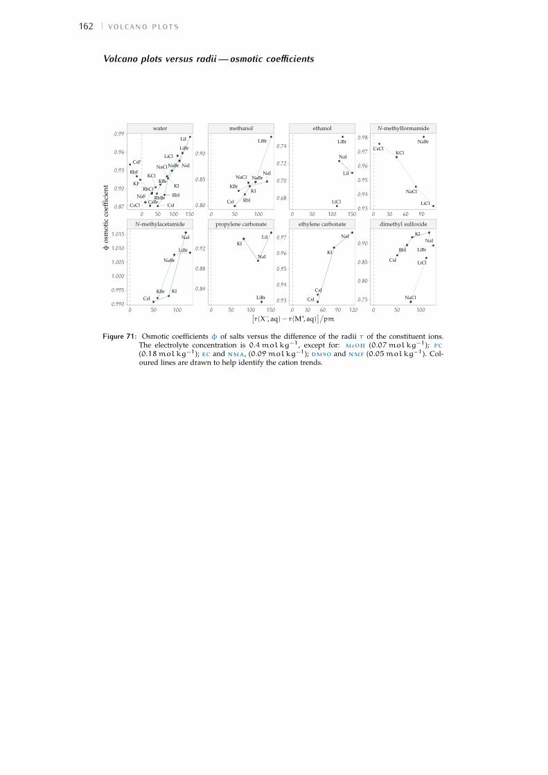
162 volcano plots
Volcano plots versus radii — osmotic coefficients
CsBrCsCl
CsF
CsI
KBrKCl
KF KI
LiBr
LiCl
LiI
NaBrNaCl
NaF
NaI
RbBr
RbCl
RbF
RbI
CsIKBr KI
LiBr
NaBr
NaI
CsI
KBrKI
LiBr
NaBrNaClNaI
RbI
KI
LiBr
LiI
NaI
LiBr
LiCl
LiI
NaI
CsI
CsI
KI
NaI
CsClKCl
LiCl
NaBr
NaCl
CsI
KI
LiBr
LiCl
NaCl
NaI
RbI
N-methylacetamide propylene carbonate ethylene carbonate dimethyl sulfoxide
water methanol ethanol N-methylformamide
0 50 100 0 50 100 150 0 30 60 90 120 0 50 100
0 50 100 150 0 50 100 0 50 100 150 0 30 60 900.93
0.94
0.95
0.96
0.97
0.98
0.75
0.80
0.85
0.90
0.68
0.70
0.72
0.74
0.93
0.94
0.95
0.96
0.97
0.80
0.85
0.90
0.84
0.88
0.92
0.87
0.90
0.93
0.96
0.99
0.990
0.995
1.000
1.005
1.010
1.015
[r(X–, aq) − r(M+, aq)
]/pm
φos
mot
icco
effic
ient
Figure 71: Osmotic coefficients φ of salts versus the difference of the radii r of the constituent ions.The electrolyte concentration is 0.4molkg−1, except for: meoh (0.07molkg−1); pc(0.18molkg−1); ec and nma, (0.09molkg−1); dmso and nmf (0.05molkg−1). Col-oured lines are drawn to help identify the cation trends.

b.2 lines highlighting cation trends 163
b.2.2 Polyatomic anions
Volcano plots versus radii — activity and osmotic coefficients
KOAc
KSCN
LiClO4
LiNO3
LiOAc
NaClO4NaForm
NaNO3
NaOAc
NaSCN
KOAc
LiForm
LiNO3
LiOAcNaNO3
KClO4
LiClO4
KClO4
LiClO4
NaClO4
water N-methylacetamide dimethyl sulfoxide sulfolane
75 100 125 150 17575 100 125 150 17575 100 125 150 17575 100 125 150 175
0.8
0.9
1.0
[r(X–, aq) − r(M+, aq)
]/pm
φos
mot
icco
effic
ient
Figure 72: Salts containing polyatomic anions. Electrolyte osmotic coefficients φ versus the differenceof the radii r of the constituent ions. The electrolyte concentration is 0.4molkg−1 for water;0.09molkg−1 for nma; 0.05molkg−1 for sulf and dmso. Coloured lines are drawnto help identify the cation trends.
KOAc
KSCN
LiClO4
LiNO3
LiOAc
NaClO4NaForm
NaNO3
NaOAc
NaSCN
KNO3
KOAc
LiForm
LiNO3
LiOAcNaFormNaNO3
NaOAc
KClO4 LiClO4
KClO4
LiClO4
NaClO4
water N-methylacetamide dimethyl sulfoxide sulfolane
60 90 120 150 60 90 120 150 60 90 120 150 60 90 120 150
0.4
0.6
0.8
[r(X–, aq) − r(M+, aq)
]/pm
γ±
mea
nac
tivi
tyco
effic
ient
Figure 73: Salts containing polyatomic anions. Electrolyte activity coefficient γ versus the difference ofthe radii r of the constituent ions. The electrolyte concentration is 0.4molkg−1 for water;0.09molkg−1 for nma; 0.05molkg−1 for sulf and dmso. Coloured lines are drawnto help identify the cation trends.

164 volcano plots
b.3 lines highlighting anion trendsb.3.1 Monoatomic ions
Classic Volcano plots — enthalpies
NaBr
NaCl
NaI
CsF
RbBr
LiBr
LiF
RbF
KIKCl
KF
CsClKBr
NaF
LiI
CsI RbICsBr
LiCl
RbCl
KCl
CsI
CsCl
NaI
NaCl
KBr
LiCl
CsBr
NaBr
KI
LiI
LiBr
CsBr
RbCl
CsI
KIKBr
NaCl
LiClNaI
KCl
LiI
LiF
NaBr
LiBr
RbBr
RbF
KF
CsF
RbI
NaF
CsCl
LiCl
RbBr
NaBr
NaI
NaF
CsF
LiBr
RbI
RbF
LiF
RbCl
KI
LiI
CsICsBr
KF
NaCl
KBrCsCl
KCl
RbI
RbBr
CsI
KBr NaBr
KCl
CsBr
LiBr
KI
LiI
NaI
CsClNaCl
RbCl
LiCl
1-propanol formamide
water methanol ethanol
0 100 200 −200 −100 0 100 200
−200 −100 0 100 200 −200 −100 0 100 200 0 100 200
−60
−30
0
−80
−60
−40
−20
0
20
−75
−50
−25
0
25
−60
−40
−20
0
20
−90
−60
−30
0
[∆abs. soln.H
−◦ (X–, g) −∆abs. soln.H−◦ (M+, g)
]/(kJmol−1)
∆so
ln.H
−◦(M
X,c
r)/(kJmol−
1)
Figure 74: Enthalpy of dissolution of salts ∆soln.H−◦ versus the difference in the absolute enthalpies of
solvation of the constituent ions ∆abs. soln.H−◦ for a range of protic solvents. Coloured lines
are drawn to help identify the anion trends.
KFRbF
CsCl
CsF
KI
NaI
LiClRbI
LiF
CsIKBr
NaF
RbCl KCl
CsBr
NaCl
LiBr
RbBr
LiI
NaBr
RbI
CsCl
LiI
LiBr
CsI
LiCl
NaClKCl
KBrRbBr
NaI
RbCl
CsBr NaBr
KI
NaCl
NaI
CsBr
CsIKI
CsCl
KBr
KCl
NaBr
KCl
KBr
CsCl
CsI
NaBr
KI LiCl
LiBr
NaCl
RbI
NaI
LiI
RbBr
RbCl
CsBr
RbI
NaCl
LiBr
CsBr
KICsCl
NaI
NaBr
LiI
KBrRbBr
KCl
CsILiCl
RbCl
dimethyl sulfoxide acetonitrile
N,N-dimethylformamide N,N-dimethylacetamide propylene carbonate
0 100 200 −50 0 50 100 150 200 250
−200 −100 0 100 200 0 50 100 150 0 50 100 150 200
−50
−25
0
25
−50
−40
−30
−20
−10
0
10
−90
−60
−30
0
−100
−75
−50
−25
0
−100
−75
−50
−25
0
[∆abs. soln.H
−◦ (X–, g) −∆abs. soln.H−◦ (M+, g)
]/(kJmol−1)
∆so
ln.H
−◦(M
X,c
r)/(kJmol−
1)
Figure 75: Enthalpy of dissolution of salts ∆soln.H−◦ versus the difference in the absolute enthalpies of
solvation of the constituent ions ∆abs. soln.H−◦ for a range of aprotic solvents. Coloured lines
are drawn to help identify the anion trends.

b.3 lines highlighting anion trends 165
Classic Volcano plots — Gibbs free energies
NaBr
NaCl
NaI
CsF
RbBr
LiBr
LiF
KI
KCl
KF
CsCl KBr
NaF
LiI
CsI
RbICsBr
LiCl
RbCl
KCl
KIKBr
NaI
NaBr
RbI
CsBr
CsCl CsI
RbBr
NaClRbCl
CsBr
RbCl
CsIKI
KBr NaCl
LiClNaI
KCl
LiI
LiF
NaBr
LiBr
RbBrKF
CsF
RbI
NaF
CsCl
NaCl
LiI
KBr
LiCl
KCl
KF
LiF
KI NaINaBr
NaF
LiBr
KFRbIRbBr
CsI
KBr
NaF
NaBr
KCl
CsBr
LiBr
KI
CsF
LiI
NaI
CsClNaCl
RbCl
LiF
LiCl
LiCl
RbBr
NaBr
NaI
NaF
CsF
LiBr
RbI
LiFRbCl
KI
LiI
CsI
CsBrKF
NaClKBr
CsCl
KCl
KCl
RbBr
CsI
CsCl
NaI
NaClKBr
LiCl
CsBr
NaBr
KI
LiI
RbCl
LiBr
RbI
1-butanol ethylene glycol formamide
water methanol ethanol 1-propanol
−50 0 50 100 −100 0 100 200 −100 0 100 200
−200 −100 0 100 200 −200 −100 0 100 200 −200 −100 0 100 200 0 100 200
−25
0
25
−30
0
30
−60
−30
0
30
−50
−25
0
25
−50
−25
0
25
−75
−50
−25
0
0
10
20
30
40
[∆abs. soln.G
−◦ (X–, g) −∆abs. soln.G−◦ (M+, g)
]/(kJmol−1)
∆so
ln.G
−◦(M
X,c
r)/(kJmol−
1)
Figure 76: Gibbs free energy of dissolution ∆soln.G−◦ of salts versus the difference in the absolute free
energies of solvation ∆abs. soln.G−◦ of the constituent ions for a range of protic solvents. Col-
oured lines are drawn to help identify the anion trends.
KF
CsCl
CsF KI
NaI
LiClRbI
LiF
CsI
KBr
NaF RbCl KCl
CsBr
NaCl
LiBr
RbBr
LiI
NaBr
RbCl
CsBr
LiI
LiBr
NaCl
LiClNaI
RbBr
CsClKBr
RbI
KCl
KI
NaBrCsI
NaCl
NaI
LiI
LiCl
RbCl
CsBr
CsI RbI
KI
LiBr
CsCl
KBr
KCl
NaBr
RbBr
RbI
CsCl
LiI
LiBr
CsILiCl
NaClKCl
KBrRbBr
NaI
RbCl
CsBrNaBr
KI
RbI
NaCl
LiBr
NaF
KF
CsBr
KICsF
CsCl
LiF
NaI
NaBr
LiI
KBr
RbBr
KCl
CsI
LiClRbCl
KCl
NaF
KBrCsCl
CsI
NaBr
KI
LiCl
LiBr
NaCl
RbICsF
LiF
KF
NaI
LiI
RbBr
RbCl
CsBr
acetone dimethyl sulfoxide acetonitrile
N,N-dimethylformamide N,N-dimethylacetamide propylene carbonate
0 50 100 150 200 0 50 100 150 200 250 −100 0 100 200
−100 0 100 200 0 100 200 −100 0 100 200
0
50
100
0
50
−75
−50
−25
0
25
−75
−50
−25
0
25
−75
−50
−25
0
25
50
−40
−20
0
20
40
60
[∆abs. soln.G
−◦ (X–, g) −∆abs. soln.G−◦ (M+, g)
]/(kJmol−1)
∆so
ln.G
−◦(M
X,c
r)/(kJmol−
1)
Figure 77: Gibbs free energy of dissolution ∆soln.G−◦ of salts versus the difference in the absolute free
energies of solvation ∆abs. soln.G−◦ of the constituent ions for a range of aprotic solvents.
Coloured lines are drawn to help identify the anion trends.
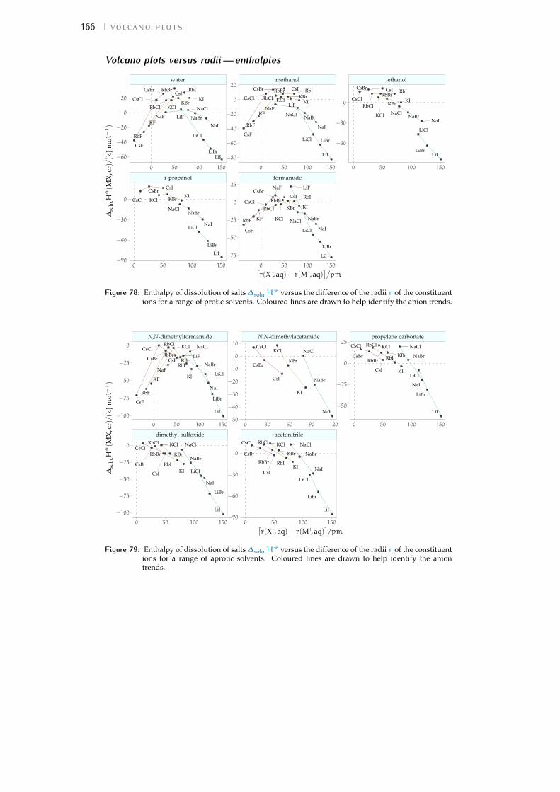
166 volcano plots
Volcano plots versus radii — enthalpies
NaBr
NaCl
NaI
CsF
RbBr
LiBr
LiF
RbF
KI
KCl
KF
CsClKBr
NaF
LiI
CsIRbICsBr
LiCl
RbCl
KCl
CsI
CsCl
NaI
NaCl
KBr
LiCl
CsBr
NaBr
KI
LiI
LiBr
CsBr
RbCl
CsI
KIKBr
NaCl
LiCl
NaI
KCl
LiI
LiF
NaBr
LiBr
RbBr
RbF
KF
CsF
RbI
NaF
CsCl
LiCl
RbBr
NaBr
NaI
NaF
CsF
LiBr
RbI
RbF
LiF
RbCl KI
LiI
CsICsBr
KF NaCl
KBrCsCl
KCl
RbIRbBr
CsI
KBr
NaBrKCl
CsBr
LiBr
KI
LiI
NaI
CsCl
NaClRbCl
LiCl
1-propanol formamide
water methanol ethanol
0 50 100 150 0 50 100 150
0 50 100 150 0 50 100 150 0 50 100 150
−60
−30
0
−80
−60
−40
−20
0
20
−75
−50
−25
0
25
−60
−40
−20
0
20
−90
−60
−30
0
[r(X–, aq) − r(M+, aq)
]/pm
∆so
ln.H
−◦(M
X,c
r)/(kJmol−
1)
Figure 78: Enthalpy of dissolution of salts∆soln.H−◦ versus the difference of the radii r of the constituent
ions for a range of protic solvents. Coloured lines are drawn to help identify the anion trends.
KF
RbF
CsCl
CsF
KI
NaI
LiCl
RbI
LiFCsI KBr
NaF
RbCl KCl
CsBr
NaCl
LiBr
RbBr
LiI
NaBr
RbI
CsCl
LiI
LiBr
CsI LiCl
NaClKCl
KBrRbBr
NaI
RbCl
CsBrNaBr
KI
NaCl
NaI
CsBr
CsI
KI
CsCl
KBr
KCl
NaBr
KCl
KBr
CsCl
CsI
NaBr
KI
LiCl
LiBr
NaCl
RbINaI
LiI
RbBr
RbCl
CsBr
RbI
NaCl
LiBr
CsBr
KI
CsCl
NaI
NaBr
LiI
KBrRbBr
KCl
CsILiCl
RbCl
dimethyl sulfoxide acetonitrile
N,N-dimethylformamide N,N-dimethylacetamide propylene carbonate
0 50 100 150 0 50 100 150
0 50 100 150 0 30 60 90 120 0 50 100 150
−50
−25
0
25
−50
−40
−30
−20
−10
0
10
−90
−60
−30
0
−100
−75
−50
−25
0
−100
−75
−50
−25
0
[r(X–, aq) − r(M+, aq)
]/pm
∆so
ln.H
−◦(M
X,c
r)/(kJmol−
1)
Figure 79: Enthalpy of dissolution of salts∆soln.H−◦ versus the difference of the radii r of the constituent
ions for a range of aprotic solvents. Coloured lines are drawn to help identify the aniontrends.

b.3 lines highlighting anion trends 167
Volcano plots versus radii — Gibbs free energies
NaBr
NaCl
NaI
CsF
RbBr
LiBr
LiF
KI
KCl
KF
CsCl
KBr
NaF
LiI
CsI
RbICsBr
LiCl
RbCl
KCl
KIKBr
NaI
NaBr
RbICsBr
CsCl
CsI
RbBr NaClRbCl
CsBr
RbCl
CsI KI
KBr NaCl
LiCl
NaI
KCl
LiI
LiF
NaBr
LiBr
RbBr
KF
CsFRbI
NaF
CsCl
NaCl
LiI
KBr
LiCl
KCl
KF
LiF
KINaI
NaBr
NaF
LiBr
KF RbIRbBr
CsI
KBr
NaF
NaBr
KClCsBr
LiBr
KICsF
LiI
NaI
CsClNaCl
RbCl
LiF
LiCl
LiCl
RbBr
NaBr NaI
NaF
CsF
LiBr
RbI
LiF
RbCl
KI
LiI
CsICsBr
KF
NaClKBrCsClKCl
KCl
RbBr
CsI
CsCl
NaI
NaClKBr
LiCl
CsBrNaBr
KI
LiI
RbCl
LiBr
RbI
1-butanol ethylene glycol formamide
water methanol ethanol 1-propanol
0 30 60 90 120 0 50 100 150 0 50 100 150
0 50 100 150 0 50 100 150 0 50 100 150 0 50 100 150
−25
0
25
−30
0
30
−60
−30
0
30
−50
−25
0
25
−50
−25
0
25
−75
−50
−25
0
0
10
20
30
40
[r(X–, aq) − r(M+, aq)
]/pm
∆so
ln.G
−◦(M
X,c
r)/(kJmol−
1)
Figure 80: Gibbs free energy of dissolution ∆soln.G−◦ of salts versus the difference of the radii r of the
constituent ions for a range of protic solvents. Coloured lines are drawn to help identify theanion trends.
KF
CsCl
CsF
KI
NaI
LiCl
RbI
LiF
CsI
KBr
NaF
RbCl
KCl
CsBr
NaCl
LiBr
RbBr
LiI
NaBr
RbCl
CsBr
LiI
LiBr
NaCl
LiCl
NaI
RbBr
CsCl
KBr
RbI
KCl
KI
NaBrCsI
NaCl
NaI
LiI
LiCl
RbCl
CsBr
CsI RbIKI
LiBr
CsClKBr
KCl
NaBrRbBr
RbI
CsCl
LiI
LiBr
CsI LiCl
NaClKClKBrRbBr
NaI
RbCl
CsBr NaBr
KI
RbI
NaCl
LiBr
NaF
KF
CsBr
KI
CsF
CsCl
LiF
NaI
NaBr
LiI
KBr
RbBr
KCl
CsI
LiCl
RbCl
KCl
NaF
KBrCsCl
CsI
NaBr
KI
LiCl
LiBr
NaCl
RbICsF
LiF
KF
NaI
LiI
RbBr
RbCl
CsBr
acetone dimethyl sulfoxide acetonitrile
N,N-dimethylformamide N,N-dimethylacetamide propylene carbonate
0 50 100 150 0 50 100 150 0 50 100 150
0 50 100 150 0 50 100 150 0 50 100 150
0
50
100
0
50
−75
−50
−25
0
25
−75
−50
−25
0
25
−75
−50
−25
0
25
50
−40
−20
0
20
40
60
[r(X–, aq) − r(M+, aq)
]/pm
∆so
ln.G
−◦(M
X,c
r)/(kJmol−
1)
Figure 81: Gibbs free energy of dissolution ∆soln.G−◦ of salts versus the difference of the radii r of the
constituent ions for a range of aprotic solvents. Coloured lines are drawn to help identify theanion trends.

168 volcano plots
Volcano plots versus radii — osmotic and activity coefficients
CsBrCsCl
CsF
CsI
KBrKCl
KF KI
LiBr
LiCl
LiI
NaBrNaCl
NaF
NaI
RbBr
RbCl
RbF
RbI
CsIKBr KI
LiBr
NaBr
NaI
CsI
KBrKI
LiBr
NaBrNaClNaI
RbI
KI
LiBr
LiI
NaI
LiBr
LiCl
LiI
NaI
CsI
CsI
KI
NaI
CsCl
KCl
LiCl
NaBr
NaCl
CsI
KI
LiBr
LiCl
NaCl
NaI
RbI
N-methylacetamide propylene carbonate ethylene carbonate dimethyl sulfoxide
water methanol ethanol N-methylformamide
0 50 100 0 50 100 150 0 30 60 90 120 0 50 100
0 50 100 150 0 50 100 0 50 100 150 0 30 60 900.93
0.94
0.95
0.96
0.97
0.98
0.75
0.80
0.85
0.90
0.68
0.70
0.72
0.74
0.93
0.94
0.95
0.96
0.97
0.80
0.85
0.90
0.84
0.88
0.92
0.87
0.90
0.93
0.96
0.99
0.990
0.995
1.000
1.005
1.010
1.015
[r(X–, aq) − r(M+, aq)
]/pm
φos
mot
icco
effic
ient
Figure 82: Osmotic coefficients φ of salts versus the difference of the radii r of the constituent ions.The electrolyte concentration is 0.4molkg−1, except for: meoh (0.07molkg−1); pc(0.18molkg−1); ec and nma, (0.09molkg−1); dmso and nmf (0.05molkg−1). Col-oured lines are drawn to help identify the anion trends.
CsBrCsCl
CsF
CsI
KBrKCl
KFKI
LiBrLiCl
LiI
NaBrNaCl
NaF
NaI
RbBr
RbCl
RbF
RbI
CsBr
CsCl CsI
KBrKClKI
LiBr
LiCl
NaBr
NaCl
NaI
CsI
KBrKI
LiBr
NaBrNaCl
NaIRbI
KI
LiBr
LiI
NaI
LiBr
LiClLiI
NaI
CsI
KI
NaI
CsCl
KCl
LiCl
NaBr
NaCl
CsI
KI
LiBr
LiCl
NaCl
NaI
RbI
N-methylacetamide propylene carbonate ethylene carbonate dimethyl sulfoxide
water methanol ethanol N-methylformamide
0 50 100 0 50 100 150 0 30 60 90 120 0 50 100
0 50 100 150 0 50 100 0 50 100 150 0 30 60 90
0.850
0.875
0.900
0.925
0.5
0.6
0.7
0.8
0.200
0.225
0.250
0.275
0.84
0.86
0.88
0.90
0.50
0.55
0.60
0.65
0.70
0.60
0.65
0.70
0.75
0.65
0.70
0.75
0.80
0.94
0.96
0.98
1.00
[r(X–, aq) − r(M+, aq)
]/pm
γ±
mea
nac
tivi
tyco
effic
ient
Figure 83: Activity coefficients γ of salts versus the difference of the radii r of the constituent ions.The electrolyte concentration is 0.4molkg−1, except for: meoh (0.07molkg−1); pc(0.18molkg−1); ec and nma, (0.09molkg−1); dmso and nmf (0.05molkg−1). Col-oured lines are drawn to help identify the anion trends.
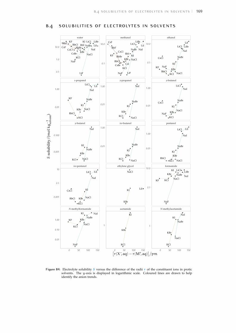
b.4 solubilities of electrolytes in solvents 169
b.4 solubilities of electrolytes in solvents
CsBr
CsClCsF
KBr
KCl
KF KI LiBrLiCl
LiF
LiINaBr
NaCl
NaF
NaIRbBr
RbClRbFRbI
KBr
KCl
KF
KI
LiClLiI
NaBr
NaCl
NaI
RbCl
KBr
KCl
KI
NaBr
NaCl
NaI
CsCl
KBr
KCl
KI
LiCl LiI
NaCl
NaI
RbCl
KBr
KCl
KF
KI
NaBr
NaCl
NaF
NaI
CsBr
CsCl
CsF
CsI
KBr
KCl
KF KI
LiBrLiCl
LiF
LiI
NaBr
NaCl
NaF
NaI
RbBr
RbCl
RbF
RbI
KBr
KCl
KI
NaBr
NaCl
NaI
KBrKCl
KI
NaBr
NaCl
NaI
KBr
KI LiI
NaCl
KBr
KCl
KI
CsCl
KBr
KCl
KFKI
LiBrLiCl
LiI
NaBr
NaCl
NaF
NaI
RbCl
CsCl
KBr
KCl
KI
LiCl
NaBr
NaClNaF
NaI
KBr
KCl
KI
LiCl LiI
NaBr
NaCl
NaI
RbCl
KBr
KClKF
KILiBr
LiCl
NaBr
NaCl
NaF
NaI
KBr
KCl
KI
NaBr
NaCl
NaI
N-methylformamide acetamide N-methylacetamide
iso-pentanol ethylene glycol formamide
2-butanol iso-butanol pentanol
1-propanol 2-propanol 2-butanol
water methanol ethanol
0 50 100 150 0 50 100 150 0 50 100 150
0.1
10.0
0.01
1.00
0.01
1.00
0.1
10.0
1
0.1
10.0
0.01
1.00
0.01
1.00
1
0.1
1.0
10.0
0.01
1.00
0.001
0.100
0.001
0.1
10
0.01
0.10
1.00
[r(X–, aq) − r(M+, aq)
]/pm
Sso
lubi
lity/
(molkg−1
solv
ent)
Figure 84: Electrolyte solubility S versus the difference of the radii r of the constituent ions in proticsolvents. The y-axis is displayed in logarithmic scale. Coloured lines are drawn to helpidentify the anion trends.
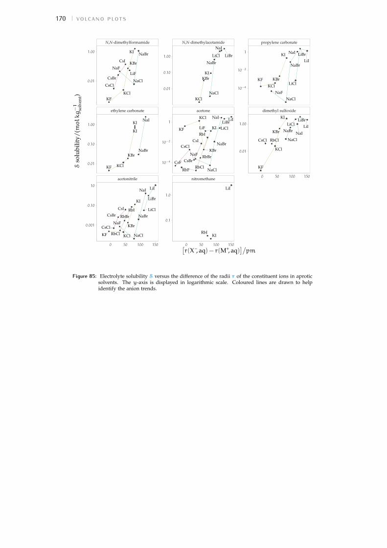
170 volcano plots
CsBr
CsCl
CsI KBr
KClKF
KI
LiF
NaBr
NaCl
NaF
KBr
KClKF
KI
KI
NaBr
NaI
CsBr
CsCl
CsI
KBr
KClKF
KI LiBr
LiCl
LiI
NaBr
NaCl
NaF
NaI
RbBr
RbCl
RbI
KBr
KCl
KI
LiBrLiCl
NaBr
NaCl
NaI
CsBr
CsCl
CsF
CsI
KBr
KCl
KF KILiBr
LiClLiF
LiI
NaBr
NaCl
NaF
NaI
RbBr
RbClRbF
RbI
KI
LiI
RbI
KBr
KCl
KF
KI LiBr
LiCl
LiINaBr
NaCl
NaF
NaI
CsCl
KBr
KCl
KF
KILiBr
LiCl LiINaBr
NaCl
NaI
RbCl
acetonitrile nitromethane
ethylene carbonate acetone dimethyl sulfoxide
N,N-dimethylformamide N,N-dimethylacetamide propylene carbonate
0 50 100 150 0 50 100 150
0 50 100 150
10−4
10−2
1
0.01
1.00
0.01
0.10
1.00
10−4
10−2
1
0.1
1.0
0.01
1.00
0.01
0.10
1.00
0.001
0.10
10
[r(X–, aq) − r(M+, aq)
]/pm
Sso
lubi
lity/
(molkg−1
solv
ent)
Figure 85: Electrolyte solubility S versus the difference of the radii r of the constituent ions in aproticsolvents. The y-axis is displayed in logarithmic scale. Coloured lines are drawn to helpidentify the anion trends.

C O S M OT I C A N D A C T I V I T Y C O E F F I -C I E N T S
c.1 fitting models and coefficientsThe Pitzer equations (Pitzer, 1973; Pitzer et al., 1973) satisfactorily represent thethermodynamic properties of electrolyte solutions up to concentrations of severalmolal, thus performing better than other models of comparable complexity andbeing widely used in chemical engineering. The most important feature introducedin this model is the ionic strength dependence of the second virial coefficient B,implying that the effect of short-range interactions between ion pairs is dependenton the ionic strength I. The Pitzer expressions for the osmotic coefficient φ and theactivity coefficient γ of a 1 : 1 electrolyte solution are:
φ− 1 = fφ +mBφ +m2Cφ [11]
lnγ = fγ +mBγ +m2Cγ [12]
where:
fφ = −AΦ√I
1+ b√I
Bφ = β(0) +β(1) exp(−α√I)
[13]
fγ = −AΦ[ √
I
1+ b√I+2
bln(1+ b
√I)]
Bγ = 2β(0) +2β(1)
α2I
[1− exp
(−α√I)(1+α
√I−
1
2α2I)]
[14]
Cγ =3
2Cφ [15]
m is the molal concentration in molkg−1;AΦ is the Debye-Hückel coefficient for the osmotic function:
AΦ =
√2πNaρ
∗s
3
√(e2
4πε0εRkT
)3
where Na is the Avogadro constant; ρ∗s is the density of the pure solvent in kgm−3;e is the elementary charge; ε0 is the vacuum permittivity; εR is the relative permit-tivity of the solvent; k is the Boltzmann constant and T is the absolute temperaturein K.I is the ionic strength:
I =1
2
∑i
mizi2
where mi is the molal concentration in molkg−1, zi the charge number of the ion i.Thus, Eqs. [11] and [12] contain five parameters that need to be fitted to experi-mental data: b, α, β(0), β(1) and Cφ. Overall, these parameters have no clear directphysical interpretation. The parameter b should remain the same for all solutes for themixed electrolytes expressions to be simple: for aqueous electrolytes, Pitzer (1973)selected the value of b = 1.2. In addition, also the same value of α = 2.0 was foundto be satisfactory for all the values fitted in Pitzer et al. (1973). For each electrolyte,
171
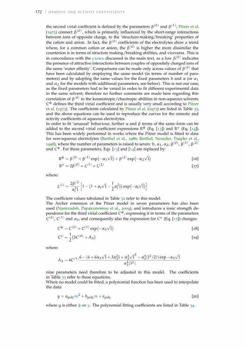
172 osmotic and activity coefficients
the second virial coefficient is defined by the parameters β(0) and β(1); Pitzer et al.(1973) connect β(0), which is primarily influenced by the short-range interactionsbetween ions of opposite charge, to the ‘structure-making/breaking’ properties ofthe cation and anion. In fact, the β(0) coefficients of the electrolytes show a trendwhere, for a common cation or anion, the β(0) is higher the more dissimilar thecounterion is in terms of structure making/breaking abilities, and viceversa. This isin concordance with the lmwa discussed in the main text, as a low β(0) indicatesthe presence of attractive interactions between couples of oppositely charged ions ofthe same ‘water affinity’. Comparisons can be made only across values of β(0) thathave been calculated by employing the same model (in terms of number of para-meters) and by adopting the same values for the fixed parameters b and α (or α1and α2 for the models with additional parameters, see below). This is not our case,as the fixed parameters had to be varied in order to fit different experimental datain the same solvent, therefore no further comments are made here regarding thiscorrelation of β(0) to the kosmotropic/chaotropic abilities in non-aqueous solvents.Cφ defines the third virial coefficient and is usually very small according to Pitzeret al. (1973). The coefficients calculated by Pitzer et al. (1973) are listed in Table 35,and the above equations can be used to reproduce the curves for the osmotic andactivity coefficients of aqueous electrolytes.In order to fit ‘unusual’ behaviour, further α and β terms of the same form can beadded to the second virial coefficient expressions Bφ (Eq. [13]) and Bγ (Eq. [14]).This has been widely performed in works where the Pitzer model is fitted to datafor non-aqueous electrolytes (Barthel et al., 1986; Barthel, Neueder, Poepke et al.,1998), where the number of parameters is raised to seven: b, α1, α2, β(0), β(1), β(2)
and Cφ. For these parameters, Eqs. [13] and [14] are replaced by:
Bφ = β(0) +β(1) exp(−α1√I)+β(2) exp
(−α2√I)
[16]
Bγ = 2β(0) + ξ(1) + ξ(2) [17]
where:
ξ(i) =2β(i)
α2i I
[1−
(1+αi
√I−
1
2α2i I)
exp(−αi√I)]
The coefficient values tabulated in Table 32 refer to this model.The Archer extension of the Pitzer model in seven parameters has also beenused (Nasirzadeh, Papaiconomou et al., 2004), and introduces a ionic strength de-pendence for the third virial coefficient Cφ, expressing it in terms of the parametersC(0), C(1) and α3, and consequently also the expression for Cγ (Eq. [15]) changes:
Cφ = C(0) +C(1) exp(−α3√I)
[18]
Cγ =1
2
(3C(0) +A3
)[19]
where:
A3 = 4C(1) 6− (6+ 6α3√I+ 3α23I+α
33
√I3−α43(I
2/2)) exp−α3√I
α43(I2)
nine parameters need therefore to be adjusted in this model. The coefficientsin Table 33 refer to these equations.Where no model could be fitted, a polynomial function has been used to interpolatethe data:
y = apolym2 + bpolym + cpoly [20]
where y is either φ or γ. The polynomial fitting coefficients are listed in Table 34.

c.1fittingmodelsandcoefficients173
Table 32: The Pitzer model fitting coefficients b, α1, α2, β(0), β(1), β(2) and Cφ in non-aqueous solvents. The osmotic and activity coefficients curves can be reproduced inthe interval comprised between mmin and mmax (in molkg−1) by employing eq. [11] and eq. [12] with Bφ and Bγ defined by eq. [16] and eq. [17].
solvent electrolyte ref. T/K fit* mmin mmax Aφ b α1 α2 β(0) β(1) β(2) Cφ σ†
2proh Bu4NBr a 298.15 Pf 0.030 1.9 2.815 3.2 2 10 0.15394 −0.44299 −18.16484 −0.00280 0.0062proh LiCl b 298.15 Pf 0.17 1.5 2.815 3.2 2 10 −0.07515 0.92283 −32.81020 0.13853 0.0042proh LiClO4 c 298.16 Pf 0.050 1.5 2.815 3.2 2 10 −0.02470 0.75212 −14.13059 0.13431 0.0062proh LiNO3 b 298.15 Pf 0.20 1.9 2.815 3.2 2 10 0.01152 0.42496 −23.19855 0.04243 0.0042proh NaI d 298.15 Pf 0.060 1.5 2.816 3.2 2 12 0.04297 0.79535 −29.90444 0.11282 0.0092proh Pent4NBr e 298.15 Pf 0.030 2.6 2.816 3.2 2 12 0.07967 0.90601 41.80878 0.03675 0.022proh Pr4NBr a 298.15 Pf 0.040 1.3 2.815 3.2 2 15 0.36167 −1.20260 −54.48017 −0.11543 0.003
ace Bu4NBr f 298.15 Pf 0.010 0.80 2.558 3.2 2 15 0.40924 −1.50268 −34.89456 −0.24477 0.004ace Bu4NClO4 f 298.15 Pf 0.020 3.6 2.558 3.2 2 10 0.06723 0.28794 2.64907 −0.00755 0.007ace LiBr f 298.15 Pf 0.030 0.80 2.558 3.2 2 13 0.34551 −0.95679 −50.46787 −0.19266 0.004ace LiClO4 g 298.16 Pf 0.010 5.9 2.558 3.2 2 20 0.06184 0.62848 −63.70265 0.03793 0.008
dma LiBr h 298.16 Pγ 0.024 0.095 1.313 3.2 2 9 0.18666 0.10206 −0.09209 3.60214 0.007
dmc LiClO4 g 298.16 Pf 0.030 1.8 51.646 95 2 20 −0.08734 −1.63671 4.11900 0.08178 0.003
dme LiClO4 g 298.16 Pf 0.010 0.40 13.545 20 2 20 −2.42556 4.02913 −1.64372 2.69628 0.007
dmf LiCl i 298.15 Pγ 0.0010 2.0 1.165 3.2 2 9 −0.27627 −0.22125 0.36039 0.13140 0.07
dmso CsI j 298.15 Pγ 0.0032 0.25 0.891 3.2 2 9 −0.32636 −0.11035 0.17095 1.32566 0.01dmso Et4NI k 298.15 P 0.0025 0.10 0.891 3.2 2 20 27.64257 −39.45606 29.87661 −69.42063 0.004dmso KCl k 298.15 P 0.0025 0.025 0.891 3.2 2 20 −56.17399 57.20798 −41.36973 329.91838 0.001dmso KClO4 l 298.15 P 0.011 0.20 0.891 3.2 2 20 1.17642 −1.62804 13.52666 −1.75351 0.002dmso KI k 298.15 P 0.0025 0.10 0.891 3.2 2 20 14.18822 −18.68884 29.25497 −38.33945 0.002dmso LiBr m 298.15 Pγ 0.027 0.86 0.891 3.2 2 9 0.24766 −0.08972 0.13331 0.10630 0.04dmso LiCl n 298.15 Pγ 0.0050 0.40 0.891 3.2 2 9 −0.41590 −0.13413 0.20351 0.67136 0.03dmso LiClO4 l 298.15 P 0.020 0.27 0.891 3.2 2 20 0.25265 0.20889 −3.01840 0.30469 0.004dmso LiI o 298.15 Pγ 0.10 0.89 0.891 3.2 2 9 0.35739 −0.08433 −0.00910 0.08310 0.02dmso NaCl k 298.15 P 0.0025 0.070 0.891 3.2 2 20 14.79014 −25.10263 −14.65969 −27.27991 0.002dmso NaI k 298.15 P 0.0025 0.10 0.891 3.2 2 20 16.57686 −22.12022 43.22616 −40.43959 0.001dmso NH4Cl k 298.15 P 0.0025 0.10 0.891 3.2 2 20 28.54137 −47.35236 −45.64717 −56.68730 0.001dmso NH4I k 298.15 P 0.0050 0.10 0.891 3.2 2 20 12.00977 −16.42490 24.35917 −30.81965 0.001
* ‘P’ Pitzer fit; ‘Pf’ Pitzer fit, already fitted in literature ref.; ‘Pγ’ Pitzer fit on γ only; † standard deviation of the residuals.a Barthel, Neueder and Wittmann, 1999; b Zafarani-Moattar et al., 2001; c Barthel, Neueder, Poepke et al., 1998; d Barthel et al., 1986; e Kunz, Turq et al., 1992;f Barthel, Neueder, Poepke et al., 1999b; g Barthel, Neueder, Poepke et al., 1999a; h Barthel, Neueder and Schröder, 1997; i Butler et al., 1970; j Archer et al., 1966;k S.-J. Kim et al., 1971; l Garnsey et al., 1968; m Salomon, 1969a; n Dunnett et al., 1965; o Salomon, 1970b; p Crawford et al., 1967; q Bonner, S. J. Kim et al., 1969;r Wood et al., 1978; s Nasehzadeh et al., 2004; t Zafarani-Moattar et al., 1999; u Bonner, Paljk et al., 1991; v Barthel et al., 1988;w Kunz, Barthel et al., 1991; x Barthel, Lauermann and Neueder, 1986; y Barthel, Neueder and Lauermann, 1985; z Nasirzadeh et al., 2004b; aa Nasirzadeh et al., 2004;bb Nasirzadeh, Papaiconomou et al., 2004; cc Zafarani-Moattar et al., 1998; dd Nasirzadeh et al., 2004a; ee Bonner, 1987; ff Nasirzadeh et al., 2003; gg Wood et al., 1971;hh Wood, Wicker et al., 1971; ii Luksha et al., 1966; jj Salomon, 1970a; kk Salomon, 1969b; ll Salomon, 1970c.

174osmoticandactivitycoefficients
solvent electrolyte ref. T/K fit* mmin mmax Aφ b α1 α2 β(0) β(1) β(2) Cφ σ†
dmso RbI p 298.15 Pγ 0.0050 0.079 0.891 3.2 2 9 0.73305 −0.14838 0.22260 −8.63804 0.005
ec CsI q 309.60 P 0.0025 0.10 0.340 3.2 2 20 9.26004 −13.43206 25.43493 −24.00216 0.003ec Et4NBr r 309.96 P 0.089 0.39 0.339 3.2 2 17 −0.57555 0.95001 −10.53603 0.58295 0.0004ec KI r 309.96 P 0.045 0.62 0.339 3.2 2 17 0.09858 0.03964 9.02385 −0.03663 0.001ec NaI r 309.96 P 0.080 0.73 0.339 3.2 2 17 0.03718 0.33362 8.01105 0.10093 0.003ec NH4I q 309.60 P 0.0025 0.10 0.340 3.2 2 20 13.21975 −20.35884 9.43814 −36.48414 0.005ec Pr4NI q 309.60 P 0.0025 0.10 0.340 3.2 2 20 7.35001 −10.08516 21.26958 −20.98049 0.004
etoh Bu4NBr a 298.15 Pf 0.050 2.5 2.005 3.2 2 10 0.16812 −0.55916 −7.58362 −0.00990 0.006etoh Et4NBr a 298.15 Pf 0.040 2.3 2.005 3.2 2 10 0.16691 −0.72983 −10.00247 −0.03198 0.01etoh LiClO4 c 298.16 Pf 0.030 1.5 2.005 3.2 2 10 0.18878 0.75994 2.69017 0.08882 0.004etoh LiI s 298.15 P 0.010 2 2.006 3.2 2 10 0.25687 0.22558 −8.15423 0.03877 0.008etoh LiNO3 t 298.15 Pf 0.12 2.1 2.006 3.2 2 1.4 1.28926 10.06746 −9.16329 −0.18575 0.005etoh Me4GuHCl u 298.15 P 0.20 3 2.006 3.2 2 10 0.18401 0.13039 15.80865 −0.02339 0.002etoh Me4GuHClO4 u 298.15 P 0.30 7 2.006 3.2 2 10 −0.07972 −0.88390 9.14798 0.00634 0.004etoh NaI d 298.15 Pf 0.040 1.9 2.007 3.2 2 20 0.15934 0.59661 5.98491 0.07164 0.01etoh Pr4NBr a 298.15 Pf 0.040 2.7 2.005 3.2 2 10 0.18176 −0.70105 −9.18950 −0.02254 0.006
mecn Bu4NBr v 298.15 Pf 0.020 2 1.112 3.2 2 20 −0.00808 −0.27186 42.66458 0.00615 0.01mecn Bu4NCl v 298.15 Pf 0.050 2.5 1.112 3.2 2 20 −0.05201 0.02315 0.67878 0.03666 0.007mecn Bu4NI v 298.15 Pf 0.050 2.4 1.112 3.2 2 12 −0.02491 −0.46604 −11.65457 0.00094 0.008mecn Et4NBr v 298.15 Pf 0.040 0.40 1.112 3.2 2 20 −0.03012 −0.78756 35.26661 −0.04900 0.007mecn LiBr w 298.15 Pf 0.020 0.84 1.112 3.2 2 7 −0.26948 −0.73717 −13.66848 0.10531 0.04mecn LiClO4 g 298.16 Pf 0.050 1.2 1.112 3.2 2 10 0.09119 −0.67565 −4.78672 −0.02324 0.004mecn NaI d 298.15 Pf 0.060 1.5 1.112 3.2 2 7 0.06190 −0.38015 −0.21550 −0.02157 0.005mecn Pent4NBr v 298.15 Pf 0.060 2.2 1.112 3.2 2 20 −0.00853 −0.19730 36.69759 0.00514 0.003mecn Pr4NBr v 298.15 Pf 0.040 1.6 1.112 3.2 2 20 0.02007 −0.64892 29.68529 −0.01611 0.005
meoh Bu4NBr x 298.15 Pf 0.040 1.7 1.295 3.2 2 20 0.11011 −0.36631 4.27136 −0.00015 0.005meoh Bu4NClO4 x 298.15 Pf 0.040 2.5 1.295 3.2 2 20 0.01071 −2.16627 −34.35735 −0.02293 0.007meoh Bu4NI x 298.15 Pf 0.040 0.90 1.295 3.2 2 20 0.45817 −2.12245 −11.65679 −0.33712 0.005meoh CsI y 298.15 Pf 0.030 0.10 1.295 3.2 2 7 −11.88200 20.15654 −11.41812 22.46690 0.004meoh Et4NBr x 298.15 Pf 0.040 1.9 1.295 3.2 2 20 0.13415 −0.74903 41.27423 −0.02968 0.007
* ‘P’ Pitzer fit; ‘Pf’ Pitzer fit, already fitted in literature ref.; ‘Pγ’ Pitzer fit on γ only; † standard deviation of the residuals.a Barthel, Neueder and Wittmann, 1999; b Zafarani-Moattar et al., 2001; c Barthel, Neueder, Poepke et al., 1998; d Barthel et al., 1986; e Kunz, Turq et al., 1992;f Barthel, Neueder, Poepke et al., 1999b; g Barthel, Neueder, Poepke et al., 1999a; h Barthel, Neueder and Schröder, 1997; i Butler et al., 1970; j Archer et al., 1966;k S.-J. Kim et al., 1971; l Garnsey et al., 1968; m Salomon, 1969a; n Dunnett et al., 1965; o Salomon, 1970b; p Crawford et al., 1967; q Bonner, S. J. Kim et al., 1969;r Wood et al., 1978; s Nasehzadeh et al., 2004; t Zafarani-Moattar et al., 1999; u Bonner, Paljk et al., 1991; v Barthel et al., 1988;w Kunz, Barthel et al., 1991; x Barthel, Lauermann and Neueder, 1986; y Barthel, Neueder and Lauermann, 1985; z Nasirzadeh et al., 2004b; aa Nasirzadeh et al., 2004;bb Nasirzadeh, Papaiconomou et al., 2004; cc Zafarani-Moattar et al., 1998; dd Nasirzadeh et al., 2004a; ee Bonner, 1987; ff Nasirzadeh et al., 2003; gg Wood et al., 1971;hh Wood, Wicker et al., 1971; ii Luksha et al., 1966; jj Salomon, 1970a; kk Salomon, 1969b; ll Salomon, 1970c.

c.1fittingmodelsandcoefficients175
solvent electrolyte ref. T/K fit* mmin mmax Aφ b α1 α2 β(0) β(1) β(2) Cφ σ†
meoh KBr y 298.15 Pf 0.040 0.10 1.295 3.2 2 7 −7.29022 12.53650 −5.90095 14.66603 0.004meoh KI y 298.15 Pf 0.030 0.80 1.295 3.2 2 7 0.10616 0.30928 0.19286 0.02324 0.003meoh KOAc z 298.15 Pf 0.17 2.5 1.294 3.2 2 3 0.07175 0.69651 −0.69345 −0.00525 0.0003meoh KSCN aa 298.15 Pf 0.13 2.7 1.294 3.2 2 1.4 −0.44378 −5.78097 5.28835 0.08060 0.005meoh LiBr bb 298.15 Pf 0.041 6.9 1.294 3.2 2 7 0.23814 0.04591 9.03892 0.02446 0.02meoh LiCl cc 298.15 Pf 0.22 4.2 1.294 3.2 2 1.4 −0.18078 −4.59638 4.00588 0.07621 0.006meoh LiClO4 dd 298.15 Pf 0.11 3.8 1.294 3.2 2 1.4 0.87847 6.35485 −5.60088 −0.07367 0.01meoh LiNO3 dd 298.15 Pf 0.12 3.8 1.294 3.2 2 1.4 0.10989 −1.81557 1.33309 0.00149 0.002meoh LiOAc cc 298.15 Pf 0.24 3.0 1.294 3.2 2 1.4 0.22018 1.60745 −1.40887 −0.01599 0.005meoh Me4GuHClO4 ee 298.15 P 0.10 8 1.293 3.2 2 10 −0.07325 −1.14389 47.81745 0.00477 0.03meoh NaBr y 298.15 Pf 0.040 1.2 1.295 3.2 2 7 −0.02214 0.88159 −0.48386 0.18579 0.002meoh NaCl y 298.15 Pf 0.040 0.20 1.295 3.2 2 7 15.38689 −29.35073 24.04528 −20.74477 0.003meoh NaClO4 y 298.15 Pf 0.060 1.3 1.295 3.2 2 7 0.21703 −0.07284 0.80089 −0.03346 0.005meoh NaI y 298.15 Pf 0.030 0.80 1.295 3.2 2 7 0.03987 0.84033 −0.60005 0.16289 0.002meoh NaOAc z 298.15 Pf 0.25 1.8 1.294 3.2 2 1.4 −0.32389 −3.22208 3.17922 0.07915 0.003meoh NaSCN ff 298.15 Pf 0.16 3.4 1.294 3.2 2 1.4 0.29789 0.45082 −0.31621 −0.02540 0.003meoh NH4SCN aa 298.15 Pf 0.23 4.4 1.294 3.2 2 1.4 0.07417 −0.89826 0.78133 −0.00878 0.009meoh Pent4NBr x 298.15 Pf 0.050 1.6 1.295 3.2 2 20 0.16323 −0.59859 −13.34552 −0.02587 0.005meoh RbI y 298.15 Pf 0.030 0.40 1.295 3.2 2 7 0.94324 −1.83339 1.89827 −0.92116 0.003
nma Bu4NBr gg 298.15 P 0.010 1 0.110 3.2 2 10 −0.06636 −0.16108 −0.11384 0.02127 0.0004nma Bu4NCl gg 298.15 P 0.010 0.90 0.110 3.2 2 9 0.14075 0.03185 −0.17784 −0.05423 0.0004nma Bu4NI gg 298.15 P 0.010 1 0.110 3.2 2 10 −0.34385 −0.40458 0.01486 0.12585 0.0002nma CsI hh 298.15 P 0.010 0.40 0.110 3.2 2 9 0.08743 0.01362 −0.10864 −0.02727 0.0003nma Et4NBr gg 298.15 P 0.010 0.90 0.110 3.2 2 10 −0.11998 −0.07594 −0.02623 −0.02350 0.0004nma Et4NCl gg 298.15 P 0.010 0.80 0.110 3.2 2 10 0.05828 0.01192 −0.14635 −0.04630 0.0003nma KBr hh 298.15 P 0.010 0.40 0.110 3.2 2 11 0.21892 −0.20202 −0.02614 −0.07325 0.0002nma KI hh 298.15 P 0.010 0.70 0.110 3.2 2 10 0.21119 −0.18936 −0.06482 0.04857 0.0003nma KOAc gg 298.15 P 0.010 0.80 0.110 3.2 2 10 0.02111 −0.05586 −0.14054 −0.02958 0.0003nma Kpropion gg 298.15 P 0.010 0.50 0.110 3.2 2 10 0.04979 0.10656 −0.28394 −0.07968 0.0003nma LiBr hh 298.15 P 0.010 0.60 0.110 3.2 2 4 0.28962 0.08052 −0.18776 0.03182 0.0002nma LiForm gg 298.15 P 0.010 0.40 0.110 3.2 2 10 −0.25520 −0.43723 −0.12733 0.25978 0.0001nma LiNO3 hh 298.15 P 0.010 0.60 0.110 3.2 2 10 0.29608 −0.15423 −0.10726 0.02638 0.0002
* ‘P’ Pitzer fit; ‘Pf’ Pitzer fit, already fitted in literature ref.; ‘Pγ’ Pitzer fit on γ only; † standard deviation of the residuals.a Barthel, Neueder and Wittmann, 1999; b Zafarani-Moattar et al., 2001; c Barthel, Neueder, Poepke et al., 1998; d Barthel et al., 1986; e Kunz, Turq et al., 1992;f Barthel, Neueder, Poepke et al., 1999b; g Barthel, Neueder, Poepke et al., 1999a; h Barthel, Neueder and Schröder, 1997; i Butler et al., 1970; j Archer et al., 1966;k S.-J. Kim et al., 1971; l Garnsey et al., 1968; m Salomon, 1969a; n Dunnett et al., 1965; o Salomon, 1970b; p Crawford et al., 1967; q Bonner, S. J. Kim et al., 1969;r Wood et al., 1978; s Nasehzadeh et al., 2004; t Zafarani-Moattar et al., 1999; u Bonner, Paljk et al., 1991; v Barthel et al., 1988;w Kunz, Barthel et al., 1991; x Barthel, Lauermann and Neueder, 1986; y Barthel, Neueder and Lauermann, 1985; z Nasirzadeh et al., 2004b; aa Nasirzadeh et al., 2004;bb Nasirzadeh, Papaiconomou et al., 2004; cc Zafarani-Moattar et al., 1998; dd Nasirzadeh et al., 2004a; ee Bonner, 1987; ff Nasirzadeh et al., 2003; gg Wood et al., 1971;hh Wood, Wicker et al., 1971; ii Luksha et al., 1966; jj Salomon, 1970a; kk Salomon, 1969b; ll Salomon, 1970c.

176osmoticandactivitycoefficients
solvent electrolyte ref. T/K fit* mmin mmax Aφ b α1 α2 β(0) β(1) β(2) Cφ σ†
nma LiOAc gg 298.15 P 0.010 0.40 0.110 3.2 2 4 −0.18794 −0.20761 −0.02212 −0.03546 0.0001nma LiPropion gg 298.15 P 0.010 0.40 0.110 3.2 2 10 −0.23605 0.11379 −0.32588 0.04235 0.0002nma Me4NCl gg 298.15 P 0.010 0.50 0.110 3.2 2 4 −0.14014 0.23817 −0.24024 −0.05610 0.0003nma NaBr hh 298.15 P 0.010 0.70 0.110 3.2 2 10 0.31070 −0.05410 −0.07537 −0.05577 0.0001nma NaI hh 298.15 P 0.010 0.80 0.110 3.2 2 10 0.39365 −0.04368 −0.12597 −0.03390 0.0003nma NaNO3 hh 298.15 P 0.010 0.80 0.110 3.2 2 10 −0.03057 −0.13199 −0.13541 −0.01015 0.0003nma NH4I q 298.15 P 0.0050 0.10 0.110 3.2 2 10 10.22854 −14.97082 −14.41121 −26.65989 0.003nma Pr4NBr gg 298.15 P 0.010 1 0.110 3.2 2 10 −0.10010 −0.17807 −0.04000 0.01948 0.0002nma Pr4NCl gg 298.15 P 0.010 0.90 0.110 3.2 2 10 0.10994 −0.03372 −0.14952 −0.04238 0.0003nma Pr4NI gg 298.15 P 0.010 0.50 0.110 3.2 2 10 −0.35273 −0.36744 0.03851 0.09576 0.0003
nmf CsCl ii 298.15 Pγ 0.010 0.070 0.112 3.2 2 9 −0.20661 −0.00140 0.00075 0.20949 0.0004nmf KCl ii 298.15 Pγ 0.010 0.070 0.112 3.2 2 9 −0.29328 −0.01205 0.01619 −1.69870 0.002nmf LiCl ii 298.15 Pγ 0.010 0.090 0.112 3.2 2 9 −1.14413 0.00581 −0.00996 1.37166 0.0006nmf NaBr ii 298.15 Pγ 0.010 0.080 0.112 3.2 2 9 −0.11352 −0.00120 0.00066 0.34003 0.0007nmf NaCl ii 298.15 Pγ 0.010 0.10 0.112 3.2 2 9 −1.52011 0.05051 −0.07437 13.95736 0.004
pc KI jj 298.15 Pγ 0.028 0.20 0.571 3.2 2 9 0.82003 −0.21855 0.46240 −2.79639 0.02pc LiBr kk 298.15 Pγ 0.13 0.65 0.571 3.2 2 9 −0.47667 −0.12361 0.56307 0.30602 0.004pc LiCl kk 298.15 Pγ 0.016 0.032 0.571 3.2 2 9 −121.59524 6.96490 −10.43926 1791.69405 0.01pc LiI jj 298.15 Pγ 0.027 0.87 0.571 3.2 2 9 0.25892 0.01739 −0.12704 0.21749 0.01pc NaI ll 298.15 Pγ 0.15 1.0 0.571 3.2 2 9 0.00420 −0.07417 0.17906 0.07742 0.010
sulf KClO4 l 298.15 P 0.0034 0.097 1.049 3.2 2 20 3.56549 −6.56617 −1.70023 −9.02753 0.002sulf LiClO4 l 298.15 P 0.0071 0.083 1.049 3.2 2 20 −3.65168 0.83212 −29.71071 18.20797 0.0007sulf NaClO4 l 298.15 P 0.0060 0.10 1.049 3.2 2 20 4.21787 −9.14430 −14.29867 −7.40667 0.002
* ‘P’ Pitzer fit; ‘Pf’ Pitzer fit, already fitted in literature ref.; ‘Pγ’ Pitzer fit on γ only; † standard deviation of the residuals.a Barthel, Neueder and Wittmann, 1999; b Zafarani-Moattar et al., 2001; c Barthel, Neueder, Poepke et al., 1998; d Barthel et al., 1986; e Kunz, Turq et al., 1992;f Barthel, Neueder, Poepke et al., 1999b; g Barthel, Neueder, Poepke et al., 1999a; h Barthel, Neueder and Schröder, 1997; i Butler et al., 1970; j Archer et al., 1966;k S.-J. Kim et al., 1971; l Garnsey et al., 1968; m Salomon, 1969a; n Dunnett et al., 1965; o Salomon, 1970b; p Crawford et al., 1967; q Bonner, S. J. Kim et al., 1969;r Wood et al., 1978; s Nasehzadeh et al., 2004; t Zafarani-Moattar et al., 1999; u Bonner, Paljk et al., 1991; v Barthel et al., 1988;w Kunz, Barthel et al., 1991; x Barthel, Lauermann and Neueder, 1986; y Barthel, Neueder and Lauermann, 1985; z Nasirzadeh et al., 2004b; aa Nasirzadeh et al., 2004;bb Nasirzadeh, Papaiconomou et al., 2004; cc Zafarani-Moattar et al., 1998; dd Nasirzadeh et al., 2004a; ee Bonner, 1987; ff Nasirzadeh et al., 2003; gg Wood et al., 1971;hh Wood, Wicker et al., 1971; ii Luksha et al., 1966; jj Salomon, 1970a; kk Salomon, 1969b; ll Salomon, 1970c.

c.1fittingmodelsandcoefficients177
Table 33: The Pitzer-Archer model fitting coefficients b, α1, α2, α3, β(0), β(1), β(2), C(0) and C(1) in non-aqueous solvents. The osmotic and activity coefficients curvescan be reproduced in the interval comprised betweenmmin andmmax (inmolkg−1) by employing eq. [11] and eq. [12] with Bφ and Bγ expressed by eq. [16]and eq. [17] and Cφ and Cγ by eq. [18] and eq. [19] respectively. The column ‘ref.’ lists the publication containing the experimental data. σ is the standarddeviation of the residuals.
solvent electrolyte ref. T/K mmin mmax Aφ b α1 α2 α3 β(0) β(1) β(2) C(0) C(1) σ
2proh LiBr a 298.15 0.074 1.5 2.816 3.2 2 7 1 1.32129 −1.73097 −3.53560 0.48349 −3.66211 0.003
etoh LiBr b 298.15 0.071 3.4 2.003 3.2 2 7 1 0.09210 0.81580 3.94757 0.10969 0.05169 0.01etoh LiCl c 298.15 0.18 3.3 2.005 3.2 2 7 1 0.42755 −0.44120 −0.21741 0.10017 −0.54095 0.004
a Nasirzadeh, Neueder and Kunz, 2005; b Nasirzadeh, Neueder and Kunz, 2004; c Safarov, 2006;
Table 34: The polynomial fitting coefficients apoly,bpoly andcpoly for data that could not be fitted by thePitzer or Pitzer-Archer models. The osmotic and activity coefficients curves can be reproducedin the interval comprised betweenmmin andmmax (in molkg−1) by employing eq. [20].
solvent electrolyte ref. T/K mmin mmax apoly bpoly cpoly
dmso CsCl a 298.15 0.0025 0.010 1720 −52.340 0.92775
ec CsI b 309.96 0.068 0.32 0.30662 −0.33668 0.96165
meoh NaNO3 c 298.15 0.050 0.75 1.0419 −1.0056 0.76416
nma CsBr d 298.15 0.010 0.20 0.53904 −0.18651 0.97795nma CsCl d 298.15 0.010 0.10 3.8333 −0.75500 0.98017nma KCl d 298.15 0.010 0.10 3.7778 −0.62667 0.97989nma KNO3 d 298.15 0.010 0.20 1.5171 −0.86303 0.97622nma LiCl d 298.15 0.010 0.30 0.11402 0.45568 0.97420nma NaCl d 298.15 0.010 0.30 0.77443 −0.013011 0.96583nma NaForm e 298.15 0.010 0.20 0.97435 −0.92422 0.97712nma NaOAc e 298.15 0.010 0.40 0.68281 −0.82602 0.96883nma NaPropion e 298.15 0.010 0.30 0.68060 −0.61659 0.97318
sulf RbClO4 f 298.15 0.0031 0.029 104.05 −7.4179 0.96274a S.-J. Kim et al., 1971; b Wood et al., 1978; c Bonner, 1987; d Wood, Wicker et al., 1971;e Wood et al., 1971; f Garnsey et al., 1968;

178osmoticandactivitycoefficients
Table 35: The Pitzer coefficients b,α,β(0),β(1) and Cφ in water as tabulated by Pitzer et al. (1973). The osmotic andactivity coefficients curves can be reproduced in the interval comprised betweenmmin andmmax (in molkg−1)by employing eq. [11] and eq. [12]. σ is the standard deviation of the residuals.
solvent electrolyte T/K mmin mmax Aφ b α β(0) β(1) Cφ σ
water Bu4NBr 298.15 0.00001 4.5 0.392 1.2 2 −0.0558 −0.5790 −0.00100 0.007water Bu4NCl 298.15 0.00001 2.5 0.392 1.2 2 0.2058 −0.4640 −0.05880 0.001water CsBr 298.15 0.00001 5 0.392 1.2 2 0.0279 0.0139 0.00004 0.002water CsCl 298.15 0.00001 5 0.392 1.2 2 0.0300 0.0558 0.00038 0.002water CsF 298.15 0.00001 3.2 0.392 1.2 2 0.1306 0.2570 −0.00430 0.002water CsI 298.15 0.00001 3 0.392 1.2 2 0.0244 0.0262 −0.00365 0.001water Et4NBr 298.15 0.00001 4 0.392 1.2 2 −0.4570 −0.4480 0.01350 0.001water Et4NCl 298.15 0.00001 3 0.392 1.2 2 0.0336 −0.1530 0.00840 0.002water Et4NI 298.15 0.00001 2 0.392 1.2 2 −0.1930 −0.5990 0.04010 0.007water KBr 298.15 0.00001 5.5 0.392 1.2 2 0.0569 0.2212 −0.00180 0.001water KCl 298.15 0.00001 4.8 0.392 1.2 2 0.0484 0.2122 −0.00084 0.0005water KF 298.15 0.00001 2 0.392 1.2 2 0.0809 0.2021 0.00093 0.001water KI 298.15 0.00001 4.5 0.392 1.2 2 0.0746 0.2517 −0.00414 0.001water KOAc 298.15 0.00001 3.5 0.392 1.2 2 0.1587 0.3251 −0.00660 0.001water KSCN 298.15 0.00001 5 0.392 1.2 2 0.0416 0.2302 −0.00252 0.001water LiBr 298.15 0.00001 2.5 0.392 1.2 2 0.1748 0.2547 0.00530 0.002water LiCl 298.15 0.00001 6 0.392 1.2 2 0.1494 0.3074 0.00359 0.001water LiClO4 298.15 0.00001 3.5 0.392 1.2 2 0.1973 0.3996 0.00800 0.002water LiI 298.15 0.00001 1.4 0.392 1.2 2 0.2104 0.3730 0 0.006water LiNO3 298.15 0.00001 6 0.392 1.2 2 0.1420 0.2780 −0.00551 0.001water LiOAc 298.15 0.00001 4 0.392 1.2 2 0.1124 0.2483 −0.00525water Me4NCl 298.15 0.00001 3.4 0.392 1.2 2 0.0149 −0.0830 0.00570 0.005water NaBr 298.15 0.00001 4 0.392 1.2 2 0.0973 0.2791 0.00116 0.004water NaCl 298.15 0.00001 6 0.392 1.2 2 0.0765 0.2664 0.00127 0.001water NaClO4 298.15 0.00001 6 0.392 1.2 2 0.0554 0.2755 −0.00118 0.001water NaF 298.15 0.00001 1 0.392 1.2 2 0.0215 0.2107 0 0.001water NaForm 298.15 0.00001 3.5 0.392 1.2 2 0.0820 0.2872 −0.00523 0.001water NaI 298.15 0.00001 3.5 0.392 1.2 2 0.1195 0.3439 0.00180 0.001water NaNO3 298.15 0.00001 6 0.392 1.2 2 0.0068 0.1783 −0.00072 0.001water NaOAc 298.15 0.00001 3.5 0.392 1.2 2 0.1426 0.3237 −0.00629 0.001water NaPropion 298.15 0.00001 3 0.392 1.2 2 0.1875 0.2789 −0.01277 0.001water NaSCN 298.15 0.00001 4 0.392 1.2 2 0.1005 0.3582 −0.00303 0.001water NH4Cl 298.15 0.00001 6 0.392 1.2 2 0.0522 0.1918 −0.00301 0.001

c.1fittingmodelsandcoefficients179
solvent electrolyte T/K mmin mmax Aφ b α β(0) β(1) Cφ σ
water NH4I 298.15 0.00001 7.5 0.392 1.2 2 0.0570 0.3157 −0.00308water Pr4NBr 298.15 0.00001 3.5 0.392 1.2 2 0.0108 −0.8260 0.00780 0.003water Pr4NCl 298.15 0.00001 2.5 0.392 1.2 2 0.1065 −0.3540 0.00980 0.002water Pr4NI 298.15 0.00001 0.50 0.392 1.2 2 −0.2839 −0.8630 0 0.005water RbBr 298.15 0.00001 5 0.392 1.2 2 0.0396 0.1530 −0.00144 0.001water RbCl 298.15 0.00001 5 0.392 1.2 2 0.0441 0.1483 −0.00101 0.001water RbF 298.15 0.00001 3.5 0.392 1.2 2 0.1141 0.2842 −0.10500 0.002water RbI 298.15 0.00001 5 0.392 1.2 2 0.0397 0.1330 −0.00108 0.001
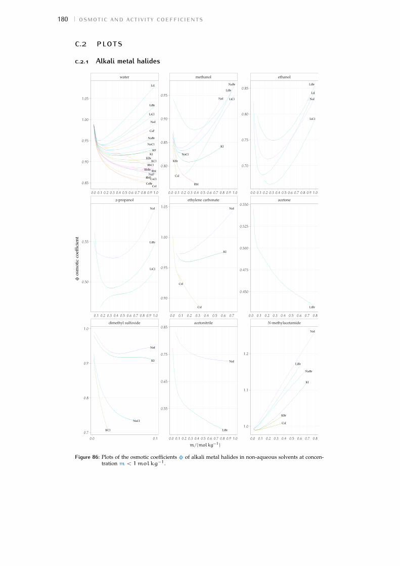
180 osmotic and activity coefficients
c.2 plotsc.2.1 Alkali metal halides
CsBr
CsCl
CsF
CsI
KBrKCl
KFKI
LiBr
LiCl
LiI
NaBr
NaCl
NaF
NaI
RbBr
RbCl
RbF
RbI
LiBr
LiCl
NaI
KCl
KI
NaCl
NaI
CsI
KBr
KI
LiBr
LiCl
NaBr
NaCl
NaI
RbI
CsI
KI
NaI
CsI
LiBr
NaI
LiBr
LiCl
LiI
NaI
LiBr
CsI
KBr
KI
LiBr
NaBr
NaI
dimethyl sulfoxide acetonitrile N-methylacetamide
2-propanol ethylene carbonate acetone
water methanol ethanol
0.0 0.1 0.0 0.1 0.2 0.3 0.4 0.5 0.6 0.7 0.8 0.9 1.0 0.0 0.1 0.2 0.3 0.4 0.5 0.6 0.7 0.8
0.1 0.2 0.3 0.4 0.5 0.6 0.7 0.8 0.9 1.0 0.0 0.1 0.2 0.3 0.4 0.5 0.6 0.7 0.0 0.1 0.2 0.3 0.4 0.5 0.6 0.7 0.8
0.0 0.1 0.2 0.3 0.4 0.5 0.6 0.7 0.8 0.9 1.0 0.0 0.1 0.2 0.3 0.4 0.5 0.6 0.7 0.8 0.9 1.0 0.0 0.1 0.2 0.3 0.4 0.5 0.6 0.7 0.8 0.9 1.0
0.70
0.75
0.80
0.85
0.450
0.475
0.500
0.525
0.550
1.0
1.1
1.2
0.80
0.85
0.90
0.95
0.90
0.95
1.00
1.05
0.55
0.65
0.75
0.85
0.85
0.90
0.95
1.00
1.05
0.50
0.55
0.7
0.8
0.9
1.0
m/(molkg−1)
φos
mot
icco
effic
ient
Figure 86: Plots of the osmotic coefficients φ of alkali metal halides in non-aqueous solvents at concen-tration m < 1molkg−1.
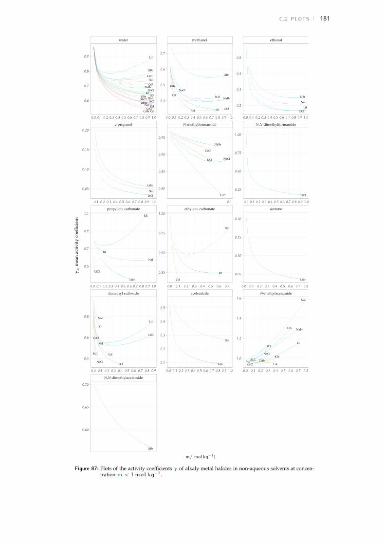
c.2 plots 181
CsBrCsCl
CsF
CsI
KBr
KCl
KFKI
LiBr
LiCl
LiI
NaBrNaCl
NaF
NaI
RbBrRbCl RbF
RbI
LiBr
LiCl
NaI
KI
LiBr
LiCl
LiI
NaI
CsIKCl
KI
LiBr
LiCl
LiI
NaCl
NaI
RbI
CsCl
LiBr
CsI
KBr
KI
LiBr
LiCl
NaBr
NaCl
NaI
RbI
CsCl
KCl
LiCl
NaBr
NaCl
CsI
KI
NaI
LiBr
NaI
LiBr
LiClLiI
NaI
LiCl
LiBr
CsI
KBr
KI
LiBr NaBr
NaI
CsBrCsCl
KCl
LiCl
NaCl
N,N-dimethylacetamide
dimethyl sulfoxide acetonitrile N-methylacetamide
propylene carbonate ethylene carbonate acetone
2-propanol N-methylformamide N,N-dimethylformamide
water methanol ethanol
0.0 0.1 0.2 0.3 0.4 0.5 0.6 0.7 0.8 0.9 0.0 0.1 0.2 0.3 0.4 0.5 0.6 0.7 0.8 0.9 1.0 0.0 0.1 0.2 0.3 0.4 0.5 0.6 0.7 0.8
0.0 0.1 0.2 0.3 0.4 0.5 0.6 0.7 0.8 0.9 1.0 0.0 0.1 0.2 0.3 0.4 0.5 0.6 0.7 0.0 0.1 0.2 0.3 0.4 0.5 0.6 0.7 0.8
0.1 0.2 0.3 0.4 0.5 0.6 0.7 0.8 0.9 1.0 0.1 0.0 0.1 0.2 0.3 0.4 0.5 0.6 0.7 0.8 0.9 1.0
0.0 0.1 0.2 0.3 0.4 0.5 0.6 0.7 0.8 0.9 1.0 0.0 0.1 0.2 0.3 0.4 0.5 0.6 0.7 0.8 0.9 1.0 0.0 0.1 0.2 0.3 0.4 0.5 0.6 0.7 0.8 0.9 1.0
0.2
0.3
0.4
0.5
0.25
0.50
0.75
1.00
0.05
0.10
0.15
0.20
1.0
1.2
1.4
1.6
0.4
0.5
0.6
0.7
0.80
0.85
0.90
0.95
0.85
0.90
0.95
1.00
0.1
0.2
0.3
0.4
0.5
0.6
0.7
0.8
0.9
0.05
0.10
0.15
0.20
0.5
0.7
0.9
1.1
0.4
0.6
0.8
0.60
0.65
0.70
m/(molkg−1)
γ±
mea
nac
tivi
tyco
effic
ient
Figure 87: Plots of the activity coefficients γ of alkaly metal halides in non-aqueous solvents at concen-tration m < 1molkg−1.
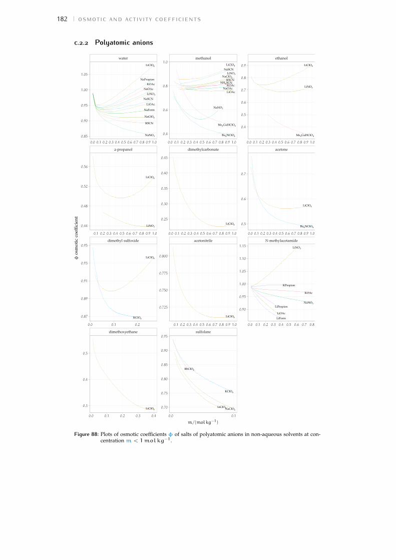
182 osmotic and activity coefficients
c.2.2 Polyatomic anions
KOAc
KSCN
LiClO4
LiNO3
LiOAc
NaClO4
NaForm
NaNO3
NaOAc
NaPropion
NaSCN
LiClO4
LiNO3
KClO4
LiClO4
LiClO4
Bu4NClO4
KOAc
KSCN
LiClO4
LiNO3
LiOAc
Me4GuHClO4
NaClO4
NaOAc
NaSCN
NH4SCN
NaNO3
LiClO4
LiClO4
KClO4
LiClO4NaClO4
RbClO4
LiClO4
LiNO3
Me4GuHClO4
Bu4NClO4
LiClO4
KOAc
KPropion
LiForm
LiNO3
LiOAc
LiPropionNaNO3
dimethoxyethane sulfolane
dimethyl sulfoxide acetonitrile N-methylacetamide
2-propanol dimethylcarbonate acetone
water methanol ethanol
0.0 0.1 0.2 0.3 0.4 0.0 0.1
0.0 0.1 0.2 0.1 0.2 0.3 0.4 0.5 0.6 0.7 0.8 0.9 1.0 0.0 0.1 0.2 0.3 0.4 0.5 0.6 0.7 0.8
0.1 0.2 0.3 0.4 0.5 0.6 0.7 0.8 0.9 1.0 0.0 0.1 0.2 0.3 0.4 0.5 0.6 0.7 0.8 0.9 1.0 0.0 0.1 0.2 0.3 0.4 0.5 0.6 0.7 0.8 0.9 1.0
0.0 0.1 0.2 0.3 0.4 0.5 0.6 0.7 0.8 0.9 1.0 0.0 0.1 0.2 0.3 0.4 0.5 0.6 0.7 0.8 0.9 1.0 0.0 0.1 0.2 0.3 0.4 0.5 0.6 0.7 0.8 0.9 1.0
0.4
0.5
0.6
0.7
0.8
0.9
0.5
0.6
0.7
0.90
0.95
1.00
1.05
1.10
1.15
0.4
0.6
0.8
1.0
0.25
0.30
0.35
0.40
0.45
0.725
0.750
0.775
0.800
0.70
0.75
0.80
0.85
0.90
0.95
0.85
0.90
0.95
1.00
1.05
0.44
0.48
0.52
0.56
0.87
0.89
0.91
0.93
0.95
0.3
0.4
0.5
m/(molkg−1)
φos
mot
icco
effic
ient
Figure 88: Plots of osmotic coefficients φ of salts of polyatomic anions in non-aqueous solvents at con-centration m < 1molkg−1.
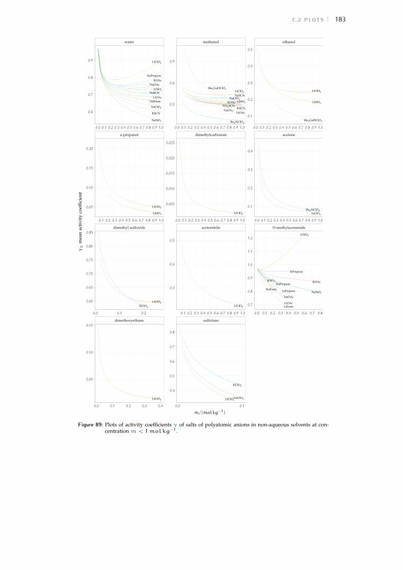
c.2 plots 183
KOAc
KSCN
LiClO4
LiNO3
LiOAc
NaClO4
NaForm
NaNO3
NaOAc
NaPropion
NaSCN
LiClO4
LiNO3
KClO4
LiClO4
LiClO4
Bu4NClO4
KOAc
KSCN
LiClO4
LiNO3
LiOAc
Me4GuHClO4
NaClO4
NaOAc
NaSCN
NH4SCN
LiClO4
LiClO4
KClO4
LiClO4NaClO4
LiClO4
LiNO3
Me4GuHClO4
Bu4NClO4LiClO4
KOAc
KPropion
LiForm
LiNO3
LiOAc
LiPropion NaNO3
KNO3
NaForm
NaOAc
NaPropion
dimethoxyethane sulfolane
dimethyl sulfoxide acetonitrile N-methylacetamide
2-propanol dimethylcarbonate acetone
water methanol ethanol
0.0 0.1 0.2 0.3 0.4 0.0 0.1
0.0 0.1 0.2 0.1 0.2 0.3 0.4 0.5 0.6 0.7 0.8 0.9 1.0 0.0 0.1 0.2 0.3 0.4 0.5 0.6 0.7 0.8
0.1 0.2 0.3 0.4 0.5 0.6 0.7 0.8 0.9 1.0 0.0 0.1 0.2 0.3 0.4 0.5 0.6 0.7 0.8 0.9 1.0 0.0 0.1 0.2 0.3 0.4 0.5 0.6 0.7 0.8 0.9 1.0
0.0 0.1 0.2 0.3 0.4 0.5 0.6 0.7 0.8 0.9 1.0 0.0 0.1 0.2 0.3 0.4 0.5 0.6 0.7 0.8 0.9 1.0 0.0 0.1 0.2 0.3 0.4 0.5 0.6 0.7 0.8 0.9 1.0
0.1
0.2
0.3
0.4
0.5
0.1
0.2
0.3
0.4
0.7
0.8
0.9
1.0
1.1
1.2
0.3
0.6
0.9
0.005
0.010
0.015
0.020
0.025
0.3
0.4
0.5
0.4
0.5
0.6
0.7
0.8
0.6
0.7
0.8
0.9
0.05
0.10
0.15
0.20
0.60
0.65
0.70
0.75
0.80
0.85
0.05
0.10
0.15
m/(molkg−1)
γ±
mea
nac
tivi
tyco
effic
ient
Figure 89: Plots of activity coefficients γ of salts of polyatomic anions in non-aqueous solvents at con-centration m < 1molkg−1.

184 osmotic and activity coefficients
c.2.3 Polyatomic cations
Bu4NBr
Bu4NCl
Et4NBr
Et4NCl
Et4NI
Me4NCl
NH4Cl
NH4I
Pr4NBr
Pr4NCl
Pr4NI
Bu4NBr
Pent4NBr
Pr4NBr
Et4NI
NH4Cl
NH4I
Bu4NBr
Bu4NClO4
Bu4NI
Et4NBr
Me4GuHClO4
NH4SCN
Pent4NBr
Et4NBr
NH4I
Pr4NI
Bu4NBr
Bu4NCl
Bu4NI
Et4NBr
Pent4NBr
Pr4NBr
Bu4NBr
Et4NBr
Me4GuHCl
Me4GuHClO4
Pr4NBr
Bu4NBr
Bu4NClO4
Bu4NBr
Bu4NCl
Bu4NI
Et4NBr
Et4NCl
Me4NCl
NH4IPr4NBr
Pr4NCl
Pr4NI
dimethyl sulfoxide acetonitrile N-methylacetamide
2-propanol ethylene carbonate acetone
water methanol ethanol
0.0 0.1 0.0 0.1 0.2 0.3 0.4 0.5 0.6 0.7 0.8 0.9 1.0 0.0 0.1 0.2 0.3 0.4 0.5 0.6 0.7 0.8 0.9 1.0
0.0 0.1 0.2 0.3 0.4 0.5 0.6 0.7 0.8 0.9 1.0 0.0 0.1 0.2 0.3 0.4 0.0 0.1 0.2 0.3 0.4 0.5 0.6 0.7 0.8 0.9 1.0
0.0 0.1 0.2 0.3 0.4 0.5 0.6 0.7 0.8 0.9 1.0 0.0 0.1 0.2 0.3 0.4 0.5 0.6 0.7 0.8 0.9 1.0 0.0 0.1 0.2 0.3 0.4 0.5 0.6 0.7 0.8 0.9 1.0
0.4
0.5
0.6
0.7
0.4
0.5
0.6
0.7
0.7
0.8
0.9
1.0
0.4
0.6
0.8
0.85
0.90
0.95
1.00
0.7
0.8
0.9
0.4
0.6
0.8
1.0
0.4
0.5
0.6
0.7
0.8
0.7
0.8
0.9
m/(molkg−1)
φos
mot
icco
effic
ient
Figure 90: Plots of osmotic coefficients φ of salts of polyatomic cations in non-aqueous solvents at con-centration m < 1molkg−1.

c.2 plots 185
Bu4NBr
Bu4NCl
Et4NBr
Et4NCl
Et4NI
Me4NCl
NH4Cl
NH4I
Pr4NBr
Pr4NCl
Pr4NI
Bu4NBr
Pent4NBr
Pr4NBr
Et4NI
NH4Cl
NH4I
Bu4NBr
Bu4NClO4
Bu4NI
Et4NBr
Me4GuHClO4
NH4SCN
Pent4NBr
Et4NBr
NH4I
Pr4NI
Bu4NBr
Bu4NCl
Bu4NI
Et4NBr
Pent4NBr
Pr4NBr
Bu4NBr
Et4NBr
Me4GuHCl
Me4GuHClO4
Pr4NBr
Bu4NBr
Bu4NClO4
Bu4NBr
Bu4NCl
Bu4NI
Et4NBr
Et4NCl
Me4NCl
NH4I
Pr4NBr
Pr4NCl
Pr4NI
dimethyl sulfoxide acetonitrile N-methylacetamide
2-propanol ethylene carbonate acetone
water methanol ethanol
0.0 0.1 0.0 0.1 0.2 0.3 0.4 0.5 0.6 0.7 0.8 0.9 1.0 0.0 0.1 0.2 0.3 0.4 0.5 0.6 0.7 0.8 0.9 1.0
0.0 0.1 0.2 0.3 0.4 0.5 0.6 0.7 0.8 0.9 1.0 0.0 0.1 0.2 0.3 0.4 0.0 0.1 0.2 0.3 0.4 0.5 0.6 0.7 0.8 0.9 1.0
0.0 0.1 0.2 0.3 0.4 0.5 0.6 0.7 0.8 0.9 1.0 0.0 0.1 0.2 0.3 0.4 0.5 0.6 0.7 0.8 0.9 1.0 0.0 0.1 0.2 0.3 0.4 0.5 0.6 0.7 0.8 0.9 1.0
0.1
0.2
0.3
0.1
0.2
0.3
0.4
0.6
0.8
1.0
0.3
0.6
0.9
0.6
0.7
0.8
0.9
1.0
0.3
0.5
0.7
0.25
0.50
0.75
1.00
0.0
0.2
0.4
0.6
0.2
0.4
0.6
0.8
m/(molkg−1)
γ±
mea
nac
tivi
tyco
effic
ient
Figure 91: Plots of activity coefficients γ of salts of polyatomic cations in non-aqueous solvents at con-centration m < 1molkg−1.
186 bibliography for the current appendix
bibliography for the current appendixArcher, M. D. and R. P. H. Gasser
1966 ‘Electrolyte Solutions in Dimethyl Sulphoxide. Part 2. — Caesium Iodide’,Trans. Faraday Soc. 62 (0 1966), pp. 3451–3458, doi: 10.1039/TF9666203451.
Barthel, J. and W. Kunz1988 ‘Vapor Pressure Data for Non-aqueous Electrolyte Solutions. Part 5. Tet-
raalkylammonium Salts in Acetonitrile’, J. Solution Chem. 17, 5, pp. 399–415, doi: 10.1007/BF00647308.
Barthel, J. and G. Lauermann1986 ‘Vapor Pressure Measurements on Non-aqueous Electrolyte Solutions.
Part 3: Solutions of Sodium Iodide in Ethanol, 2-propanol, and Acetoni-trile’, J. Solution Chem. 15, 10, pp. 869–877, doi: 10.1007/BF00646093.
Barthel, J., G. Lauermann and R. Neueder1986 ‘Vapor Pressure Measurements on Non-aqueous Electrolyte Solutions.
Part 2. Tetraalkylammonium Salts in Methanol. Activity Coefficients ofVarious 1− 1 Electrolytes at High Concentrations’, J. Solution Chem. 15, 10,pp. 851–867, doi: 10.1007/BF00646092.
Barthel, J., R. Neueder and G. Lauermann1985 ‘Vapor Pressures of Non-aqueous Electrolyte Solutions. Part 1. Alkali
Metal Salts in Methanol’, J. Solution Chem. 14, 9, pp. 621–633, doi: 10 .1007/BF00646055.
Barthel, J., R. Neueder and A. Schröder1997 ‘Temperature Dependence of Activity Coefficients and Gibbs Ener-
gies of Transfer of LiBr in Acetonitrile, Dimethyl Sulfoxide, and N,N-dimethylacetamide from EMF Measurements’, Can. J. Chem. 75, 11,pp. 1500–1507, doi: 10.1139/v97-180.
Barthel, J., R. Neueder, H. Poepke and H. Wittmann1998 ‘Osmotic and Activity Coefficients of Nonaqueous Electrolyte Solutions.
1. Lithium Perchlorate in the Protic Solvents Methanol, Ethanol, and 2-propanol’, J. Solution Chem. 27, 12, pp. 1055–1066, doi: 10.1023/A:1022637316064.
1999a ‘Osmotic Coefficients and Activity Coefficients of Nonaqueous ElectrolyteSolutions. Part 2. Lithium Perchlorate in the Aprotic Solvents Acetone,Acetonitrile, Dimethoxyethane, and Dimethylcarbonate’, J. Solution Chem.28, 5, pp. 489–503, doi: 10.1023/A:1022674613995.
1999b ‘Osmotic Coefficients and Activity Coefficients of Nonaqueous Electro-lyte Solutions. Part 4. Lithium Bromide, Tetrabutylammonium Bromide,and Tetrabutylammonium Perchlorate in Acetone’, J. Solution Chem. 28,12, pp. 1277–1287, doi: 10.1023/A:1021791823158.
Barthel, J., R. Neueder and H. Wittmann1999 ‘Osmotic Coefficients and Activity Coefficients of Nonaqueous Electro-
lyte Solutions. Part 3. Tetraalkylammonium Bromides in Ethanol and2-propanol’, J. Solution Chem. 28, 12, pp. 1263–1276, doi: 10 . 1023 / A :1021741006320.
Bonner, O. D.1987 ‘The Colligative Properties of Certain Electrolytes and Non-electrolytes in
Methanol’, J. Solution Chem. 16, 4, pp. 307–314, doi: 10.1007/BF00646122.

bibliography for the current appendix 187
Bonner, O. D., Š. Paljk and C. Klofutar1991 ‘Association Studies of Tetramethylguanidinium Perchlorate and Tetra-
methylguanidinium Chloride in Ethanol Solutions at 25 ◦C’, J. SolutionChem. 20, 5, pp. 539–550, doi: 10.1007/BF00650808.
Bonner, O. D., S. J. Kim and A. L. Torres1969 ‘Comparison of the Osmotic and Activity Coefficients of Some Solutes in
Structured Solvents’, J. Phys. Chem. 73, 6, pp. 1968–1974, doi: 10.1021/j100726a054.
Butler, J. N. and J. C. Synnott1970 ‘Thermodynamics of Lithium Chloride in Dimethylformamide’, J. Am.
Chem. Soc. 92, 9, pp. 2602–2607, doi: 10.1021/ja00712a002.
Crawford, J. M. and R. P. H. Gasser1967 ‘Electrolyte Solutions in Dimethyl Sulphoxide. Part 3.— Rubidium Iodide’,
Trans. Faraday Soc. 63 (0 1967), pp. 2758–2764, doi: 10.1039/TF9676302758.
Dunnett, J. S. and R. P. H. Gasser1965 ‘Electrolyte Solutions in Dimethyl Sulphoxide. Part 1.— Lithium Chlor-
ide’, Trans. Faraday Soc. 61 (0 1965), pp. 922–927, doi: 10 . 1039 /TF9656100922.
Garnsey, R. and J. E. Prue1968 ‘Precise Cryoscopic Determination of Osmotic Coefficients for Solutions
of Some Alkali Metal Salts in Dimethyl Sulphoxide and in Sulpholane’,Trans. Faraday Soc. 64 (0 1968), pp. 1206–1218, doi: 10.1039/TF9686401206.
Kim, S.-J., O. D. Bonner and D.-S. Shin1971 ‘Solvent-solute Interactions in Dimethylsulfoxide’, J. Chem. Thermodyn. 3,
4, pp. 411–417, doi: 10.1016/S0021-9614(71)80024-1.
Kunz, W., J. Barthel, L. Klein, T. Cartailler, P. Turq and B. Reindl1991 ‘Lithium Bromide in Acetonitrile: Thermodynamics, Theory, and Simula-
tion’, J. Solution Chem. 20, 9, pp. 875–891, doi: 10.1007/BF01074950.
Kunz, W., P. Turq, P. Calmettes, J. Barthel and L. Klein1992 ‘n-tetrapentylammonium Bromide in 2-propanol: Vapor Pressure and
Small-angle Neutron Scattering Measurements’, J. Phys. Chem. 96, 6,pp. 2743–2749, doi: 10.1021/j100185a063.
Luksha, E. and C. M. Criss1966 ‘Thermodynamic Properties of Nonaqueous Solutions. II. Free Energies,
Entropies, and Activity Coefficients of Selected Alkali Metal Halides inAnhydrous N-Methylformamide’, J. Phys. Chem. 70, 5, pp. 1496–1502, doi:10.1021/j100877a026.
Nasehzadeh, A., E. Noroozian and H. Omrani2004 ‘Experimental and Theoretical Studies of Thermodynamics of Lithium
Halide Solutions — Ethanol Mixtures’, J. Chem. Thermodyn. 36, 3, pp. 245–252, doi: 10.1016/j.jct.2003.12.002.
Nasirzadeh, K. and R. Neueder2004a ‘Measurement and Correlation of Osmotic Coefficients and Evaluation of
Vapor Pressure for Electrolyte Solutions of LiClO4 and LiNO3 in Methanolat 25 ◦C’, J. Mol. Liq. 113, 1, pp. 13–20, doi: 10.1016/j.molliq.2004.02.028.
2004b ‘Measurements and Correlation of Osmotic Coefficients and Evaluation ofVapor Pressure for Solutions of KCH3COO and NaCH3COO in Methanolat 25 ◦C’, Acta Chim. Slov. 51, 1, pp. 117–126, http://acta-arhiv.chem-soc.si/51/51-1-117.pdf.
188 bibliography for the current appendix
Nasirzadeh, K., R. Neueder and W. Kunz2004 ‘Vapor Pressures, Osmotic and Activity Coefficients of Electrolytes in
Protic Solvents at Different Temperatures. 2. Lithium Bromide in Ethanol’,J. Solution Chem. 33, 11, pp. 1429–1446, issn: 1572-8927, doi: 10.1007/s10953-004-1057-9.
2005 ‘Vapor Pressures, Osmotic and Activity Coefficients of Electrolytes inProtic Solvents at Different Temperatures. 3. Lithium Bromide in 2-propanol’, J. Solution Chem. 34, 1, pp. 9–24, issn: 1572-8927, doi: 10.1007/s10953-005-2024-9.
Nasirzadeh, K., N. Papaiconomou, R. Neueder and W. Kunz2004 ‘Vapor Pressures, Osmotic and Activity Coefficients of Electrolytes in
Protic Solvents at Different Temperatures. 1. Lithium Bromide in Meth-anol’, J. Solution Chem. 33, 3, pp. 227–245, doi: 10 . 1023 / B : JOSL .0000035357.18045.0d.
Nasirzadeh, K. and A. Salabat2003 ‘Isopiestic Determination of Osmotic Coefficients and Evaluation of Vapor
Pressures for Solutions of Sodium Bromide and Sodium Thiocyanate inMethanol at 25 ◦C’, J. Mol. Liq. 106, 1, pp. 1–14, doi: 10.1016 /S0167-7322(03)00016-3.
Nasirzadeh, K. and M. T. Zafarani-Moattar2004 ‘Isopiestic Determination of Osmotic Coefficients and Evaluation of Vapor
Pressures for Solutions of KI, NH4SCN and KSCN in Methanol at 25 ◦C’,J. Mol. Liq. 111, 1, pp. 7–13, doi: 10.1016/j.molliq.2003.08.021.
Pitzer, K. S.1973 ‘Thermodynamics of Electrolytes. I. Theoretical Basis and General Equa-
tions’, J. Phys. Chem. 77, 2, pp. 268–277, doi: 10.1021/j100621a026.
Pitzer, K. S. and G. Mayorga1973 ‘Thermodynamics of Electrolytes. II. Activity and Osmotic Coefficients for
Strong Electrolytes with One or Both Ions Univalent’, J. Phys. Chem. 77, 19,pp. 2300–2308, doi: 10.1021/j100638a009.
Safarov, J. T.2006 ‘Vapor Pressures of Lithium Bromide or Lithium Chloride and Ethanol
Solutions’, Fluid Phase Equilib. 243, 1-2, pp. 38–44, doi: 10.1016/j.fluid.2006.02.012.
Salomon, M.1969a ‘Thermodynamics of LiBr in Anhydrous Dimethyl Sulfoxide’, J. Electro-
chem. Soc. 116, 10, pp. 1392–1394, doi: 10.1149/1.2411530.1969b ‘Thermodynamics of Lithium Chloride and Lithium Bromide in Propyl-
ene Carbonate’, J. Phys. Chem. 73, 10, pp. 3299–3306, doi: 10 . 1021 /j100844a026.
1970a ‘Thermodynamics of Lithium and Potassium Iodide in Anhydrous Propyl-ene Carbonate’, J. Electroanal. Chem. Interfacial Electrochem. 26, 2, pp. 319–329, doi: 10.1016/S0022-0728(70)80315-1.
1970b ‘Thermodynamics of Lithium Iodide in Anhydrous Dimethyl Sulfoxide’,J. Electrochem. Soc. 117, 3, pp. 325–328, doi: 10.1149/1.2407502.
1970c ‘Thermodynamics of Sodium Iodide in Propylene Carbonate’, J. Elec-troanal. Chem. Interfacial Electrochem. 25, 1, pp. 1–8, doi: 10.1016/S0022-0728(70)80033-X.

bibliography for the current appendix 189
Wood, R. H. and R. W. Kreis1971 ‘Freezing Points, Osmotic Coefficients, and Activity Coefficients of Salts
in N-Methylacetamide. II. Tetraalkylammonium Halides and Some AlkaliMetal Formates, Acetates, and Propionates’, J. Phys. Chem. 75, 15, pp. 2319–2325, doi: 10.1021/j100684a015.
Wood, R. H., R. K. Wicker and R. W. Kreis1971 ‘Freezing Points, Osmotic Coefficients, and Activity Coefficients of Salts
in N-Methylacetamide. I. Alkali Halides and Nitrates’, J. Phys. Chem. 75,15, pp. 2313–2318, doi: 10.1021/j100684a014.
Wood, R. H. and Q. D. Craft1978 ‘Freezing Points, Osmotic Coefficients, and Activity Coefficients of Some
Salts in Ethylene Carbonate: A High Dielectric Constant Solvent withoutHydrogen Bonding’, J. Solution Chem. 7, 11, pp. 799–812, doi: 10.1007/BF00650809.
Zafarani-Moattar, M. T. and M. Aria2001 ‘Isopiestic Determination of Osmotic and Activity Coefficients for Solu-
tions Of ce LiCl, LiBr, and LiNO3 in 2-propanol at 25 ◦C’, J. Solution Chem.30, 4, pp. 351–363, doi: 10.1023/A:1010327206913.
Zafarani-Moattar, M. T. and J. Jahanbin-Sardroodi1999 ‘Isopiestic Determination of Osmotic Coefficients and Evaluation of Vapor
Pressures for Electrolyte Solutions of Some Lithium Salts in Ethanol’, FluidPhase Equilib. 166, 2, pp. 207–223, doi: 10.1016/S0378-3812(99)00293-9.
Zafarani-Moattar, M. T. and K. Nasirzade1998 ‘Osmotic Coefficient of Methanol + LiCl, + LiBr, and + LiCH3COO at
25 ◦C’, J. Chem. Eng. Data, 43, 2, pp. 215–219, doi: 10.1021/je970193e.

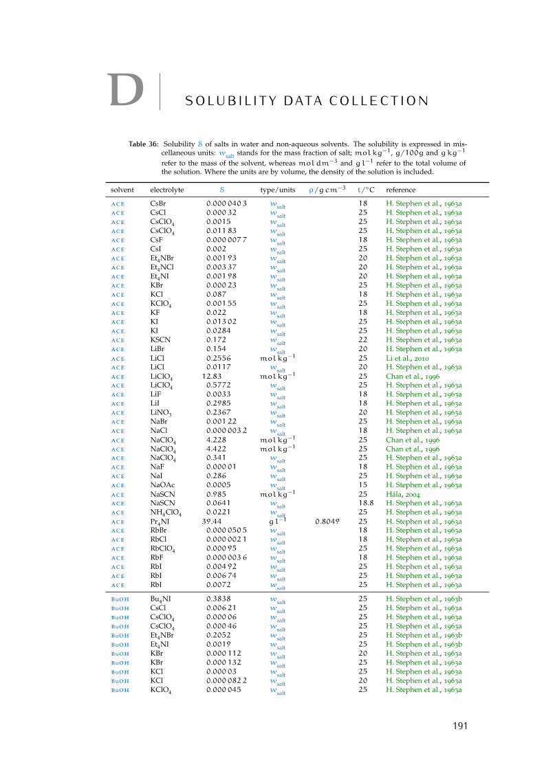
D S O L U B I L I T Y DATA C O L L E C T I O N
Table 36: Solubility S of salts in water and non-aqueous solvents. The solubility is expressed in mis-cellaneous units: wsalt stands for the mass fraction of salt; molkg−1, g/100g and gkg−1
refer to the mass of the solvent, whereas moldm−3 and gl−1 refer to the total volume ofthe solution. Where the units are by volume, the density of the solution is included.
solvent electrolyte S type/units ρ/gcm−3 t/◦C reference
ace CsBr 0.0000403 wsalt 18 H. Stephen et al., 1963aace CsCl 0.00032 wsalt 25 H. Stephen et al., 1963aace CsClO4 0.0015 wsalt 25 H. Stephen et al., 1963aace CsClO4 0.01183 wsalt 25 H. Stephen et al., 1963aace CsF 0.0000077 wsalt 18 H. Stephen et al., 1963aace CsI 0.002 wsalt 25 H. Stephen et al., 1963aace Et4NBr 0.00193 wsalt 20 H. Stephen et al., 1963aace Et4NCl 0.00337 wsalt 20 H. Stephen et al., 1963aace Et4NI 0.00198 wsalt 20 H. Stephen et al., 1963aace KBr 0.00023 wsalt 25 H. Stephen et al., 1963aace KCl 0.087 wsalt 18 H. Stephen et al., 1963aace KClO4 0.00155 wsalt 25 H. Stephen et al., 1963aace KF 0.022 wsalt 18 H. Stephen et al., 1963aace KI 0.01302 wsalt 25 H. Stephen et al., 1963aace KI 0.0284 wsalt 25 H. Stephen et al., 1963aace KSCN 0.172 wsalt 22 H. Stephen et al., 1963aace LiBr 0.154 wsalt 20 H. Stephen et al., 1963aace LiCl 0.2556 molkg−1 25 Li et al., 2010ace LiCl 0.0117 wsalt 20 H. Stephen et al., 1963aace LiClO4 12.83 molkg−1 25 Chan et al., 1996ace LiClO4 0.5772 wsalt 25 H. Stephen et al., 1963aace LiF 0.0033 wsalt 18 H. Stephen et al., 1963aace LiI 0.2985 wsalt 18 H. Stephen et al., 1963aace LiNO3 0.2367 wsalt 20 H. Stephen et al., 1963aace NaBr 0.00122 wsalt 25 H. Stephen et al., 1963aace NaCl 0.0000032 wsalt 18 H. Stephen et al., 1963aace NaClO4 4.228 molkg−1 25 Chan et al., 1996ace NaClO4 4.422 molkg−1 25 Chan et al., 1996ace NaClO4 0.341 wsalt 25 H. Stephen et al., 1963aace NaF 0.00001 wsalt 18 H. Stephen et al., 1963aace NaI 0.286 wsalt 25 H. Stephen et al., 1963aace NaOAc 0.0005 wsalt 15 H. Stephen et al., 1963aace NaSCN 0.985 molkg−1 25 Hála, 2004ace NaSCN 0.0641 wsalt 18.8 H. Stephen et al., 1963aace NH4ClO4 0.0221 wsalt 25 H. Stephen et al., 1963aace Pr4NI 39.44 gl−1 0.8049 25 H. Stephen et al., 1963aace RbBr 0.0000505 wsalt 18 H. Stephen et al., 1963aace RbCl 0.0000021 wsalt 18 H. Stephen et al., 1963aace RbClO4 0.00095 wsalt 25 H. Stephen et al., 1963aace RbF 0.0000036 wsalt 18 H. Stephen et al., 1963aace RbI 0.00492 wsalt 25 H. Stephen et al., 1963aace RbI 0.00674 wsalt 25 H. Stephen et al., 1963aace RbI 0.0072 wsalt 25 H. Stephen et al., 1963a
buoh Bu4NI 0.3838 wsalt 25 H. Stephen et al., 1963bbuoh CsCl 0.00621 wsalt 25 H. Stephen et al., 1963abuoh CsClO4 0.00006 wsalt 25 H. Stephen et al., 1963abuoh CsClO4 0.00046 wsalt 25 H. Stephen et al., 1963abuoh Et4NBr 0.2052 wsalt 25 H. Stephen et al., 1963bbuoh Et4NI 0.0019 wsalt 25 H. Stephen et al., 1963bbuoh KBr 0.000112 wsalt 20 H. Stephen et al., 1963abuoh KBr 0.000132 wsalt 25 H. Stephen et al., 1963abuoh KCl 0.00003 wsalt 25 H. Stephen et al., 1963abuoh KCl 0.0000822 wsalt 20 H. Stephen et al., 1963abuoh KClO4 0.000045 wsalt 25 H. Stephen et al., 1963a
191
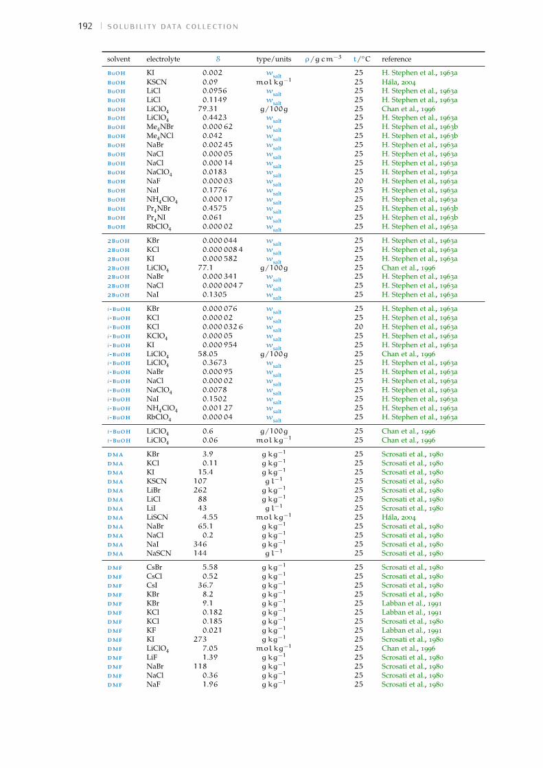
192 solubility data collection
solvent electrolyte S type/units ρ/gcm−3 t/◦C reference
buoh KI 0.002 wsalt 25 H. Stephen et al., 1963abuoh KSCN 0.09 molkg−1 25 Hála, 2004buoh LiCl 0.0956 wsalt 25 H. Stephen et al., 1963abuoh LiCl 0.1149 wsalt 25 H. Stephen et al., 1963abuoh LiClO4 79.31 g/100g 25 Chan et al., 1996buoh LiClO4 0.4423 wsalt 25 H. Stephen et al., 1963abuoh Me4NBr 0.00062 wsalt 25 H. Stephen et al., 1963bbuoh Me4NCl 0.042 wsalt 25 H. Stephen et al., 1963bbuoh NaBr 0.00245 wsalt 25 H. Stephen et al., 1963abuoh NaCl 0.00005 wsalt 25 H. Stephen et al., 1963abuoh NaCl 0.00014 wsalt 25 H. Stephen et al., 1963abuoh NaClO4 0.0183 wsalt 25 H. Stephen et al., 1963abuoh NaF 0.00003 wsalt 20 H. Stephen et al., 1963abuoh NaI 0.1776 wsalt 25 H. Stephen et al., 1963abuoh NH4ClO4 0.00017 wsalt 25 H. Stephen et al., 1963abuoh Pr4NBr 0.4575 wsalt 25 H. Stephen et al., 1963bbuoh Pr4NI 0.061 wsalt 25 H. Stephen et al., 1963bbuoh RbClO4 0.00002 wsalt 25 H. Stephen et al., 1963a
2buoh KBr 0.000044 wsalt 25 H. Stephen et al., 1963a2buoh KCl 0.0000084 wsalt 25 H. Stephen et al., 1963a2buoh KI 0.000582 wsalt 25 H. Stephen et al., 1963a2buoh LiClO4 77.1 g/100g 25 Chan et al., 19962buoh NaBr 0.000341 wsalt 25 H. Stephen et al., 1963a2buoh NaCl 0.0000047 wsalt 25 H. Stephen et al., 1963a2buoh NaI 0.1305 wsalt 25 H. Stephen et al., 1963a
i-buoh KBr 0.000076 wsalt 25 H. Stephen et al., 1963ai-buoh KCl 0.00002 wsalt 25 H. Stephen et al., 1963ai-buoh KCl 0.0000326 wsalt 20 H. Stephen et al., 1963ai-buoh KClO4 0.00005 wsalt 25 H. Stephen et al., 1963ai-buoh KI 0.000954 wsalt 25 H. Stephen et al., 1963ai-buoh LiClO4 58.05 g/100g 25 Chan et al., 1996i-buoh LiClO4 0.3673 wsalt 25 H. Stephen et al., 1963ai-buoh NaBr 0.00095 wsalt 25 H. Stephen et al., 1963ai-buoh NaCl 0.00002 wsalt 25 H. Stephen et al., 1963ai-buoh NaClO4 0.0078 wsalt 25 H. Stephen et al., 1963ai-buoh NaI 0.1502 wsalt 25 H. Stephen et al., 1963ai-buoh NH4ClO4 0.00127 wsalt 25 H. Stephen et al., 1963ai-buoh RbClO4 0.00004 wsalt 25 H. Stephen et al., 1963a
t-buoh LiClO4 0.6 g/100g 25 Chan et al., 1996t-buoh LiClO4 0.06 molkg−1 25 Chan et al., 1996
dma KBr 3.9 gkg−1 25 Scrosati et al., 1980dma KCl 0.11 gkg−1 25 Scrosati et al., 1980dma KI 15.4 gkg−1 25 Scrosati et al., 1980dma KSCN 107 gl−1 25 Scrosati et al., 1980dma LiBr 262 gkg−1 25 Scrosati et al., 1980dma LiCl 88 gkg−1 25 Scrosati et al., 1980dma LiI 43 gl−1 25 Scrosati et al., 1980dma LiSCN 4.55 molkg−1 25 Hála, 2004dma NaBr 65.1 gkg−1 25 Scrosati et al., 1980dma NaCl 0.2 gkg−1 25 Scrosati et al., 1980dma NaI 346 gkg−1 25 Scrosati et al., 1980dma NaSCN 144 gl−1 25 Scrosati et al., 1980
dmf CsBr 5.58 gkg−1 25 Scrosati et al., 1980dmf CsCl 0.52 gkg−1 25 Scrosati et al., 1980dmf CsI 36.7 gkg−1 25 Scrosati et al., 1980dmf KBr 8.2 gkg−1 25 Scrosati et al., 1980dmf KBr 9.1 gkg−1 25 Labban et al., 1991dmf KCl 0.182 gkg−1 25 Labban et al., 1991dmf KCl 0.185 gkg−1 25 Scrosati et al., 1980dmf KF 0.021 gkg−1 25 Labban et al., 1991dmf KI 273 gkg−1 25 Scrosati et al., 1980dmf LiClO4 7.05 molkg−1 25 Chan et al., 1996dmf LiF 1.39 gkg−1 25 Scrosati et al., 1980dmf NaBr 118 gkg−1 25 Scrosati et al., 1980dmf NaCl 0.36 gkg−1 25 Scrosati et al., 1980dmf NaF 1.96 gkg−1 25 Scrosati et al., 1980

solubility data collection 193
solvent electrolyte S type/units ρ/gcm−3 t/◦C reference
dmf NaSCN 295 gkg−1 25 Scrosati et al., 1980dmf NH4Br 147 gkg−1 25 Scrosati et al., 1980dmf NH4I 459 gkg−1 25 Scrosati et al., 1980dmf NH4SCN 154 gkg−1 25 Scrosati et al., 1980
dmso CsCl 0.0373 molkg−1 25 Butler, 1967dmso KBr 50.3 gkg−1 25 Labban et al., 1991dmso KBr 0.5 molkg−1 25 Butler, 1967dmso KCl 1.96 gkg−1 25 Labban et al., 1991dmso KCl 0.0225 molkg−1 25 Butler, 1967dmso KClO4 2.5 molkg−1 25 Butler, 1967dmso KF 0.023 gkg−1 25 Labban et al., 1991dmso KI 2.5 molkg−1 25 Butler, 1967dmso LiBr 3.3 molkg−1 25 Butler, 1967dmso LiCl 2.13 molkg−1 25 Butler, 1967dmso LiCl 2.2 molkg−1 25 Butler, 1967dmso LiClO4 21.1 g/100g 25 Chan et al., 1996dmso LiClO4 2.65 molkg−1 25 Butler, 1967dmso LiClO4 2.7 molkg−1 25 Butler, 1967dmso LiClO4 2.7 molkg−1 25 Chan et al., 1996dmso LiI 1.22 molkg−1 25 Butler, 1967dmso LiI 2.8 molkg−1 25 Butler, 1967dmso NaBr 0.55 molkg−1 25 Butler, 1967dmso NaCl 0.078 molkg−1 25 Butler, 1967dmso NaCl 0.08 molkg−1 25 Butler, 1967dmso NaClO4 1.8 molkg−1 25 Butler, 1967dmso NaClO4 1.8 molkg−1 25 Chan et al., 1996dmso NaI 1 molkg−1 25 Butler, 1967dmso RbCl 0.0356 molkg−1 25 Butler, 1967
ec KBr 0.0185 molkg−1 40 Peruzzi, Ninham et al., 2012ec KCl 0.0115 molkg−1 40 Peruzzi, Ninham et al., 2012ec KClO4 0.2779 molkg−1 40 Peruzzi, Ninham et al., 2012ec KF 0.0045 molkg−1 40 Peruzzi, Ninham et al., 2012ec KI 0.671 molkg−1 40 Harris, 1958ec KI 0.6969 molkg−1 40 Peruzzi, Ninham et al., 2012ec KI 0.8512 molkg−1 25 Peruzzi, Ninham et al., 2012ec KNO3 0.0248 molkg−1 40 Peruzzi, Ninham et al., 2012ec KSCN 0.0034 molkg−1 25 Peruzzi, Ninham et al., 2012ec LiClO4 96.7 g/100g 25 Chan et al., 1996ec Me4NI 2.4 gl−1 1.0678 25 H. Stephen et al., 1963aec NaBr 0.03 molkg−1 40 Harris, 1958ec NaI 2.51 molkg−1 40 Harris, 1958
eg KBr 0.1342 wsalt 25 H. Stephen et al., 1963beg KI 0.3301 wsalt 25 H. Stephen et al., 1963aeg KI 0.3329 wsalt 25 H. Stephen et al., 1963beg LiI 0.28 wsalt 15.3 H. Stephen et al., 1963aeg NaCl 0.317 wsalt 14.8 H. Stephen et al., 1963aeg NaClO4 6.166 molkg−1 25 Chan et al., 1996
etoh CsCl 0.07697 wsalt 25 H. Stephen et al., 1963aetoh CsClO4 0.00011 wsalt 25 H. Stephen et al., 1963aetoh CsClO4 0.00093 wsalt 25 H. Stephen et al., 1963aetoh Et4NBr 0.346 wsalt 20 H. Stephen et al., 1963aetoh Et4NCl 0.576 wsalt 20 H. Stephen et al., 1963aetoh Et4NI 0.00914 wsalt 20 H. Stephen et al., 1963aetoh KBr 0.00135 wsalt 25 H. Stephen et al., 1963aetoh KBr 0.00142 wsalt 25 H. Stephen et al., 1963aetoh KBr 0.00453 wsalt 20 H. Stephen et al., 1963aetoh KCl 0.0064 molkg−1 25 Li et al., 2010etoh KCl 0.00022 wsalt 25 H. Stephen et al., 1963aetoh KCl 0.000294 wsalt 25 H. Stephen et al., 1963aetoh KCl 0.00034 wsalt 25 Pinho et al., 2005etoh KClO4 0.00012 wsalt 25 H. Stephen et al., 1963aetoh KF 0.0191 molkg−1 25 Labban et al., 1997etoh KF 0.00106 wsalt 20 H. Stephen et al., 1963aetoh KI 0.0172 wsalt 20.5 H. Stephen et al., 1963aetoh KI 0.0184 wsalt 25 H. Stephen et al., 1963aetoh KI 0.01922 wsalt 25 H. Stephen et al., 1963a
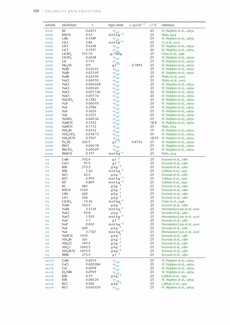
194 solubility data collection
solvent electrolyte S type/units ρ/gcm−3 t/◦C reference
etoh KI 0.0211 wsalt 25 H. Stephen et al., 1963aetoh KSCN 0.53 molkg−1 25 Hála, 2004etoh LiBr 0.4189 wsalt 25 H. Stephen et al., 1963aetoh LiCl 5.84 molkg−1 25 Li et al., 2010etoh LiCl 0.0248 wsalt 25 H. Stephen et al., 1963aetoh LiCl 0.1957 wsalt 20 H. Stephen et al., 1963aetoh LiClO4 151.76 g/100g 25 Chan et al., 1996etoh LiClO4 0.6028 wsalt 25 H. Stephen et al., 1963aetoh LiI 0.715 wsalt 25 H. Stephen et al., 1963aetoh Me4NI 0.9 gl−1 0.7894 25 H. Stephen et al., 1963aetoh NaBr 0.02261 wsalt 25 H. Stephen et al., 1963aetoh NaBr 0.02349 wsalt 25 H. Stephen et al., 1963aetoh NaBr 0.02496 wsalt 25 Pinho et al., 2005etoh NaCl 0.00055 wsalt 25 Pinho et al., 2005etoh NaCl 0.000648 wsalt 25 H. Stephen et al., 1963aetoh NaCl 0.00065 wsalt 25 H. Stephen et al., 1963aetoh NaCl 0.001146 wsalt 20 H. Stephen et al., 1963aetoh NaCl 0.00176 wsalt 20 H. Stephen et al., 1963aetoh NaClO4 0.1282 wsalt 25 H. Stephen et al., 1963aetoh NaF 0.00095 wsalt 20 H. Stephen et al., 1963aetoh NaI 0.2986 wsalt 25 H. Stephen et al., 1963aetoh NaI 0.3023 wsalt 25 H. Stephen et al., 1963aetoh NaI 0.3151 wsalt 25 H. Stephen et al., 1963aetoh NaNO3 0.00036 wsalt 25 H. Stephen et al., 1963aetoh NaSCN 0.1552 wsalt 18.8 H. Stephen et al., 1963aetoh NaSCN 0.1712 wsalt 25 Hála, 2004etoh NH4Br 0.0312 wsalt 19 H. Stephen et al., 1963aetoh NH4ClO4 0.01872 wsalt 25 H. Stephen et al., 1963aetoh NH4SCN 0.1907 wsalt 18.45 H. Stephen et al., 1963aetoh Pr4NI 202.9 gl−1 0.8716 25 H. Stephen et al., 1963aetoh RbCl 0.00078 wsalt 25 H. Stephen et al., 1963aetoh RbClO4 0.00009 wsalt 25 H. Stephen et al., 1963aetoh RbSCN 0.197 molkg−1 25 Hála, 2004
fa CsBr 152.4 gl−1 25 Scrosati et al., 1980fa CsCl 91.5 gl−1 25 Scrosati et al., 1980fa KBr 215.3 gkg−1 25 Scrosati et al., 1980fa KBr 1.26 molkg−1 25 Labban et al., 1997fa KCl 62.3 gkg−1 25 Scrosati et al., 1980fa KCl 0.995 molkg−1 25 Labban et al., 1997fa KF 0.869 molkg−1 25 Labban et al., 1997fa KI 683 gkg−1 25 Scrosati et al., 1980fa KSCN 1420 gkg−1 25 Scrosati et al., 1980fa LiBr 600 gkg−1 25 Scrosati et al., 1980fa LiCl 266 gkg−1 25 Scrosati et al., 1980fa LiClO4 13.36 molkg−1 25 Chan et al., 1996fa NaBr 353.4 gkg−1 25 Scrosati et al., 1980fa NaBr 3.3134 molkg−1 25 Hernández-Luis et al., 2016fa NaCl 93.8 gkg−1 25 Scrosati et al., 1980fa NaCl 1.555 molkg−1 25 Hernández-Luis et al., 2016fa NaF 1.1 gl−1 25 Scrosati et al., 1980fa NaF 0.002 molkg−1 25 Hernández-Luis et al., 2016fa NaI 600 gkg−1 25 Scrosati et al., 1980fa NaI 3.7767 molkg−1 25 Hernández-Luis et al., 2016fa NaSCN 1435 gkg−1 25 Scrosati et al., 1980fa NH4Br 361 gkg−1 25 Scrosati et al., 1980fa NH4Cl 109.5 gkg−1 25 Scrosati et al., 1980fa NH4I 1043.5 gkg−1 25 Scrosati et al., 1980fa NH4SCN 1015.5 gkg−1 25 Scrosati et al., 1980fa RbBr 274.5 gl−1 25 Scrosati et al., 1980
mecn CsBr 0.0014 wsalt 25 H. Stephen et al., 1963amecn CsCl 0.000084 wsalt 25 H. Stephen et al., 1963amecn CsI 0.0098 wsalt 25 H. Stephen et al., 1963amecn Et4NBr 0.0959 wsalt 25 H. Stephen et al., 1963amecn KBr 0.19 gkg−1 25 Labban et al., 1991mecn KBr 0.00024 wsalt 25 H. Stephen et al., 1963amecn KCl 0.006 gkg−1 25 Labban et al., 1991mecn KCl 0.000024 wsalt 25 H. Stephen et al., 1963a

solubility data collection 195
solvent electrolyte S type/units ρ/gcm−3 t/◦C reference
mecn KF 0.004 gkg−1 25 Labban et al., 1991mecn KF 0.000024 wsalt 25 H. Stephen et al., 1963amecn KI 0.02003 wsalt 24 H. Stephen et al., 1963amecn KI 0.0206 wsalt 25 H. Stephen et al., 1963amecn KSCN 0.1023 wsalt 18 H. Stephen et al., 1963amecn LiBr 0.081 wsalt 25 H. Stephen et al., 1963amecn LiCl 0.0014 wsalt 25 H. Stephen et al., 1963amecn LiClO4 12.99 g/100g 25 Chan et al., 1996mecn LiClO4 13.6 g/100g 25 Chan et al., 1996mecn LiClO4 14.46 g/100g 25 Chan et al., 1996mecn LiClO4 1.4 molkg−1 25 Chan et al., 1996mecn LiClO4 1.53 molkg−1 25 Chan et al., 1996mecn LiClO4 1.5419 molkg−1 24.2 Chan et al., 1996mecn LiI 0.6063 wsalt 25 H. Stephen et al., 1963amecn LiNO3 0.029 wsalt 25 H. Stephen et al., 1963amecn NaBr 0.0004 wsalt 25 H. Stephen et al., 1963amecn NaCl 0.0000025 wsalt 25 H. Stephen et al., 1963amecn NaF 0.00003 wsalt 25 H. Stephen et al., 1963amecn NaI 0.1993 wsalt 25 H. Stephen et al., 1963amecn NaOAc 0.0014 moldm−3 0.7675 25 Soleymani et al., 2013mecn NH4SCN 0.988 molkg−1 18 Hála, 2004mecn Pr4NI 186.9 gl−1 0.8584 25 H. Stephen et al., 1963amecn RbBr 0.00047 wsalt 25 H. Stephen et al., 1963amecn RbCl 0.000036 wsalt 25 H. Stephen et al., 1963amecn RbI 0.0135 wsalt 25 H. Stephen et al., 1963amecn RbI 0.0165 wsalt 25 H. Stephen et al., 1963a
meno2 KI 0.00307 wsalt 25 H. Stephen et al., 1963ameno2 LiI 0.252 wsalt 25 H. Stephen et al., 1963ameno2 Me4NI 3.8 gl−1 1.1285 25 H. Stephen et al., 1963ameno2 Pr4NI 222.4 gl−1 1.158 25 H. Stephen et al., 1963ameno2 RbI 0.00518 wsalt 25 H. Stephen et al., 1963a
meoh Bu4NI 0.7195 wsalt 25 H. Stephen et al., 1963bmeoh CsBr 2.12 g/100g 23.3 Stenger, 1996meoh CsBr 0.022 wsalt 25 H. Stephen et al., 1963ameoh CsCl 3.26 g/100g 23.4 Stenger, 1996meoh CsCl 0.0292 wsalt 25 H. Stephen et al., 1963ameoh CsCl 0.2659 wsalt 25 H. Stephen et al., 1963ameoh CsClO4 0.086 g/100g 23.3 Stenger, 1996meoh CsClO4 0.00093 wsalt 25 H. Stephen et al., 1963ameoh CsClO4 0.00742 wsalt 25 H. Stephen et al., 1963ameoh CsF 152 g/100g 22.2 Stenger, 1996meoh CsI 3.45 g/100g 22 Stenger, 1996meoh CsI 0.0365 wsalt 25 H. Stephen et al., 1963ameoh CsNO3 0.309 g/100g 23.5 Stenger, 1996meoh Et4NBr 0.583 wsalt 20 H. Stephen et al., 1963ameoh Et4NBr 0.583 wsalt 20 H. Stephen et al., 1963ameoh Et4NBr 0.5985 wsalt 25 H. Stephen et al., 1963bmeoh Et4NCl 0.699 wsalt 20 H. Stephen et al., 1963ameoh Et4NCl 0.699 wsalt 20 H. Stephen et al., 1963ameoh Et4NI 0.0905 wsalt 20 H. Stephen et al., 1963ameoh Et4NI 0.0905 wsalt 20 H. Stephen et al., 1963ameoh Et4NI 0.1103 wsalt 25 H. Stephen et al., 1963bmeoh KBr 2.08 g/100g 25 Harner et al., 1963meoh KBr 0.0205 wsalt 25 H. Stephen et al., 1963ameoh KBr 0.0207 wsalt 25 H. Stephen et al., 1963ameoh KBr 0.0212 wsalt 25 H. Stephen et al., 1963ameoh KCl 0.5335 g/100g 25 Harner et al., 1963meoh KCl 0.0736 molkg−1 25 Li et al., 2010meoh KCl 0.0052 wsalt 25 H. Stephen et al., 1963ameoh KCl 0.0053 wsalt 25 H. Stephen et al., 1963ameoh KCl 0.005363 wsalt 25 H. Stephen et al., 1963ameoh KCl 0.00539 wsalt 25 Pinho et al., 2005meoh KCl 0.00826 wsalt 20 H. Stephen et al., 1963ameoh KClO4 0.00105 wsalt 25 H. Stephen et al., 1963ameoh KF 2.286 g/100g 25 Harner et al., 1963meoh KF 10.3 g/100g 23.4 Stenger, 1996meoh KF 0.00192 wsalt 20 H. Stephen et al., 1963ameoh KF 0.0926 wsalt 25 H. Stephen et al., 1963a
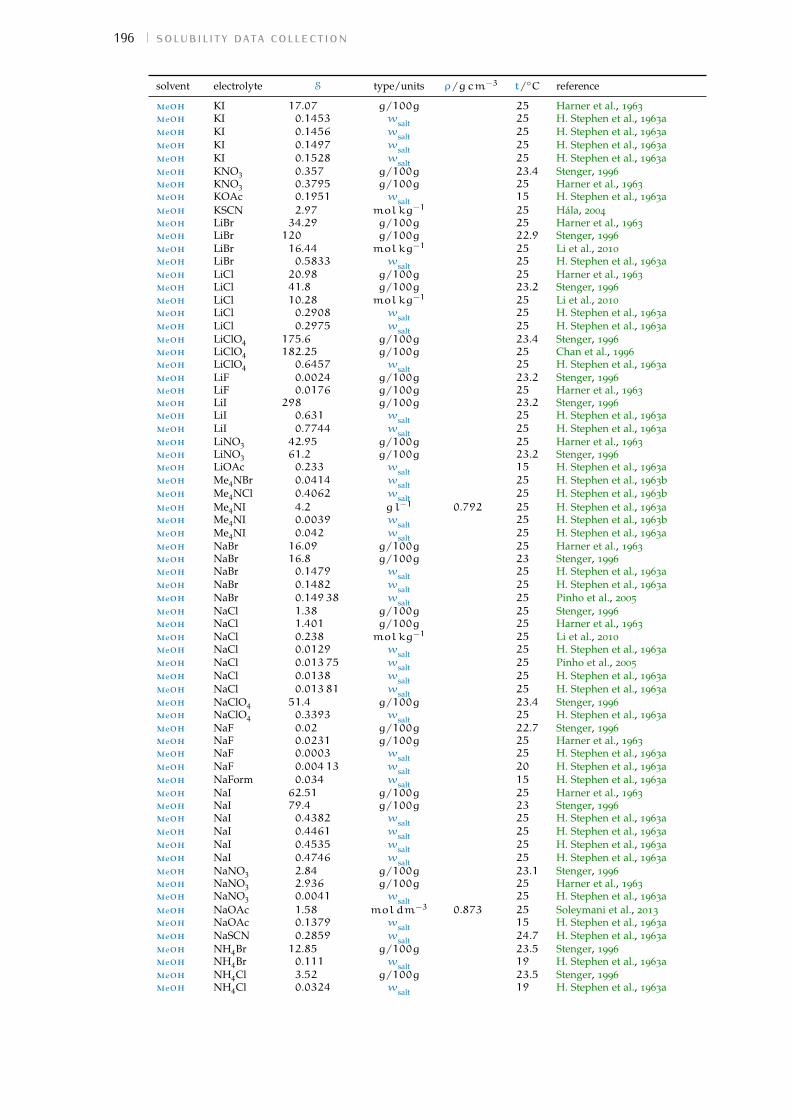
196 solubility data collection
solvent electrolyte S type/units ρ/gcm−3 t/◦C reference
meoh KI 17.07 g/100g 25 Harner et al., 1963meoh KI 0.1453 wsalt 25 H. Stephen et al., 1963ameoh KI 0.1456 wsalt 25 H. Stephen et al., 1963ameoh KI 0.1497 wsalt 25 H. Stephen et al., 1963ameoh KI 0.1528 wsalt 25 H. Stephen et al., 1963ameoh KNO3 0.357 g/100g 23.4 Stenger, 1996meoh KNO3 0.3795 g/100g 25 Harner et al., 1963meoh KOAc 0.1951 wsalt 15 H. Stephen et al., 1963ameoh KSCN 2.97 molkg−1 25 Hála, 2004meoh LiBr 34.29 g/100g 25 Harner et al., 1963meoh LiBr 120 g/100g 22.9 Stenger, 1996meoh LiBr 16.44 molkg−1 25 Li et al., 2010meoh LiBr 0.5833 wsalt 25 H. Stephen et al., 1963ameoh LiCl 20.98 g/100g 25 Harner et al., 1963meoh LiCl 41.8 g/100g 23.2 Stenger, 1996meoh LiCl 10.28 molkg−1 25 Li et al., 2010meoh LiCl 0.2908 wsalt 25 H. Stephen et al., 1963ameoh LiCl 0.2975 wsalt 25 H. Stephen et al., 1963ameoh LiClO4 175.6 g/100g 23.4 Stenger, 1996meoh LiClO4 182.25 g/100g 25 Chan et al., 1996meoh LiClO4 0.6457 wsalt 25 H. Stephen et al., 1963ameoh LiF 0.0024 g/100g 23.2 Stenger, 1996meoh LiF 0.0176 g/100g 25 Harner et al., 1963meoh LiI 298 g/100g 23.2 Stenger, 1996meoh LiI 0.631 wsalt 25 H. Stephen et al., 1963ameoh LiI 0.7744 wsalt 25 H. Stephen et al., 1963ameoh LiNO3 42.95 g/100g 25 Harner et al., 1963meoh LiNO3 61.2 g/100g 23.2 Stenger, 1996meoh LiOAc 0.233 wsalt 15 H. Stephen et al., 1963ameoh Me4NBr 0.0414 wsalt 25 H. Stephen et al., 1963bmeoh Me4NCl 0.4062 wsalt 25 H. Stephen et al., 1963bmeoh Me4NI 4.2 gl−1 0.792 25 H. Stephen et al., 1963ameoh Me4NI 0.0039 wsalt 25 H. Stephen et al., 1963bmeoh Me4NI 0.042 wsalt 25 H. Stephen et al., 1963ameoh NaBr 16.09 g/100g 25 Harner et al., 1963meoh NaBr 16.8 g/100g 23 Stenger, 1996meoh NaBr 0.1479 wsalt 25 H. Stephen et al., 1963ameoh NaBr 0.1482 wsalt 25 H. Stephen et al., 1963ameoh NaBr 0.14938 wsalt 25 Pinho et al., 2005meoh NaCl 1.38 g/100g 25 Stenger, 1996meoh NaCl 1.401 g/100g 25 Harner et al., 1963meoh NaCl 0.238 molkg−1 25 Li et al., 2010meoh NaCl 0.0129 wsalt 25 H. Stephen et al., 1963ameoh NaCl 0.01375 wsalt 25 Pinho et al., 2005meoh NaCl 0.0138 wsalt 25 H. Stephen et al., 1963ameoh NaCl 0.01381 wsalt 25 H. Stephen et al., 1963ameoh NaClO4 51.4 g/100g 23.4 Stenger, 1996meoh NaClO4 0.3393 wsalt 25 H. Stephen et al., 1963ameoh NaF 0.02 g/100g 22.7 Stenger, 1996meoh NaF 0.0231 g/100g 25 Harner et al., 1963meoh NaF 0.0003 wsalt 25 H. Stephen et al., 1963ameoh NaF 0.00413 wsalt 20 H. Stephen et al., 1963ameoh NaForm 0.034 wsalt 15 H. Stephen et al., 1963ameoh NaI 62.51 g/100g 25 Harner et al., 1963meoh NaI 79.4 g/100g 23 Stenger, 1996meoh NaI 0.4382 wsalt 25 H. Stephen et al., 1963ameoh NaI 0.4461 wsalt 25 H. Stephen et al., 1963ameoh NaI 0.4535 wsalt 25 H. Stephen et al., 1963ameoh NaI 0.4746 wsalt 25 H. Stephen et al., 1963ameoh NaNO3 2.84 g/100g 23.1 Stenger, 1996meoh NaNO3 2.936 g/100g 25 Harner et al., 1963meoh NaNO3 0.0041 wsalt 25 H. Stephen et al., 1963ameoh NaOAc 1.58 moldm−3 0.873 25 Soleymani et al., 2013meoh NaOAc 0.1379 wsalt 15 H. Stephen et al., 1963ameoh NaSCN 0.2859 wsalt 24.7 H. Stephen et al., 1963ameoh NH4Br 12.85 g/100g 23.5 Stenger, 1996meoh NH4Br 0.111 wsalt 19 H. Stephen et al., 1963ameoh NH4Cl 3.52 g/100g 23.5 Stenger, 1996meoh NH4Cl 0.0324 wsalt 19 H. Stephen et al., 1963a

solubility data collection 197
solvent electrolyte S type/units ρ/gcm−3 t/◦C reference
meoh NH4ClO4 6.67 g/100g 22.7 Stenger, 1996meoh NH4ClO4 0.0641 wsalt 25 H. Stephen et al., 1963ameoh NH4F 2.61 g/100g 23.3 Stenger, 1996meoh NH4I 59.8 g/100g 23.4 Stenger, 1996meoh NH4NO3 18.4 g/100g 23.4 Stenger, 1996meoh NH4OAc 0.0731 wsalt 15 H. Stephen et al., 1963ameoh NH4SCN 0.3711 wsalt 24.58 H. Stephen et al., 1963ameoh Pr4NBr 0.7288 wsalt 25 H. Stephen et al., 1963bmeoh Pr4NI 564.2 gl−1 1.0187 25 H. Stephen et al., 1963ameoh Pr4NI 0.5728 wsalt 25 H. Stephen et al., 1963bmeoh RbBr 2.48 g/100g 23.2 Stenger, 1996meoh RbBr 0.0246 wsalt 25 H. Stephen et al., 1963ameoh RbCl 1.36 g/100g 23.4 Stenger, 1996meoh RbCl 0.0132 wsalt 25 H. Stephen et al., 1963ameoh RbCl 0.0139 wsalt 25 H. Stephen et al., 1963ameoh RbClO4 0.054 g/100g 22.8 Stenger, 1996meoh RbClO4 0.0006 wsalt 25 H. Stephen et al., 1963ameoh RbF 69.7 g/100g 23 Stenger, 1996meoh RbI 10.8 g/100g 23.3 Stenger, 1996meoh RbI 0.1 wsalt 25 H. Stephen et al., 1963ameoh RbNO3 0.46 g/100g 23.4 Stenger, 1996meoh RbSCN 1.377 molkg−1 25 Hála, 2004
nma KBr 50.03 gkg−1 40 Scrosati et al., 1980nma KCl 9.58 gkg−1 40 Scrosati et al., 1980nma KI 316.6 gkg−1 40 Scrosati et al., 1980nma KSCN 210.88 gl−1 40 Scrosati et al., 1980nma LiCl 17.51 gl−1 40 Scrosati et al., 1980nma NaBr 192.31 gkg−1 40 Scrosati et al., 1980nma NaCl 21.09 gkg−1 40 Scrosati et al., 1980nma NaI 562.7 gkg−1 40 Scrosati et al., 1980nma NaSCN 295.1 gl−1 40 Scrosati et al., 1980nma NH4Br 221.1 gkg−1 40 Scrosati et al., 1980nma NH4Cl 50.93 gkg−1 40 Scrosati et al., 1980nma NH4I 358 gl−1 40 Scrosati et al., 1980nma NH4SCN 352.1 gl−1 40 Scrosati et al., 1980
nmf KBr 101.7 gkg−1 25 Scrosati et al., 1980nmf KBr 0.468 molkg−1 25 Labban et al., 1997nmf KCl 22.4 gkg−1 25 Scrosati et al., 1980nmf KCl 0.354 molkg−1 25 Labban et al., 1997nmf KF 0.616 molkg−1 25 Labban et al., 1997nmf KI 491 gkg−1 25 Scrosati et al., 1980nmf KSCN 809 gkg−1 25 Scrosati et al., 1980nmf NaBr 298 gkg−1 25 Scrosati et al., 1980nmf NaBr 2.9286 molkg−1 25 Hernández-Luis et al., 2016nmf NaCl 32.6 gkg−1 25 Scrosati et al., 1980nmf NaCl 0.55 molkg−1 25 Hernández-Luis et al., 2016nmf NaF 0.002 molkg−1 25 Hernández-Luis et al., 2016nmf NaI 787 gkg−1 25 Scrosati et al., 1980nmf NaI 5.1973 molkg−1 25 Hernández-Luis et al., 2016nmf NaSCN 503 gkg−1 25 Scrosati et al., 1980nmf NH4Cl 58 gkg−1 25 Scrosati et al., 1980nmf NH4I 380 gkg−1 25 Scrosati et al., 1980nmf NH4SCN 744 gkg−1 25 Scrosati et al., 1980
pc CsBr 0.0098 moldm−3 25 Muhuri et al., 1993pc CsCl 0.0076 moldm−3 25 Muhuri et al., 1993pc CsClO4 0.052 moldm−3 25 Muhuri et al., 1993pc KBr 0.003 moldm−3 25 Muhuri et al., 1993pc KBr 0.0006 molkg−1 25 Harris, 1958pc KBr 0.00398 molkg−1 25 Peruzzi, Lo Nostro et al., 2015pc KCl 0.00058 moldm−3 25 Muhuri et al., 1993pc KCl 0.000367 molkg−1 25 Peruzzi, Lo Nostro et al., 2015pc KCl 0.0004 molkg−1 25 Harris, 1958pc KClO4 0.017 moldm−3 25 Muhuri et al., 1993pc KClO4 0.0457 molkg−1 25 Peruzzi, Lo Nostro et al., 2015pc KF 0.00017 molkg−1 25 Peruzzi, Lo Nostro et al., 2015pc KI 0.221 molkg−1 25 Peruzzi, Lo Nostro et al., 2015pc KI 0.223 molkg−1 25 Harris, 1958
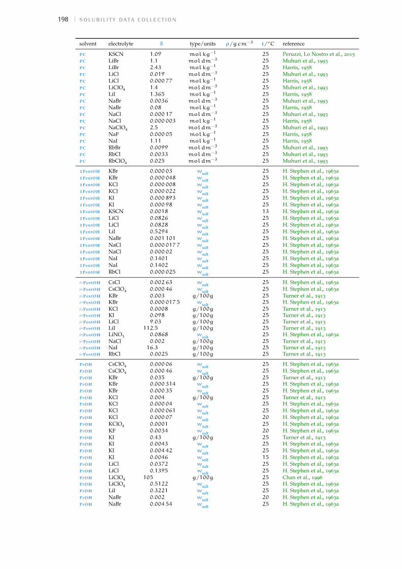
198 solubility data collection
solvent electrolyte S type/units ρ/gcm−3 t/◦C reference
pc KSCN 1.09 molkg−1 25 Peruzzi, Lo Nostro et al., 2015pc LiBr 1.1 moldm−3 25 Muhuri et al., 1993pc LiBr 2.43 molkg−1 25 Harris, 1958pc LiCl 0.019 moldm−3 25 Muhuri et al., 1993pc LiCl 0.00077 molkg−1 25 Harris, 1958pc LiClO4 1.4 moldm−3 25 Muhuri et al., 1993pc LiI 1.365 molkg−1 25 Harris, 1958pc NaBr 0.0036 moldm−3 25 Muhuri et al., 1993pc NaBr 0.08 molkg−1 25 Harris, 1958pc NaCl 0.00017 moldm−3 25 Muhuri et al., 1993pc NaCl 0.000003 molkg−1 25 Harris, 1958pc NaClO4 2.5 moldm−3 25 Muhuri et al., 1993pc NaF 0.00005 molkg−1 25 Harris, 1958pc NaI 1.11 molkg−1 25 Harris, 1958pc RbBr 0.0099 moldm−3 25 Muhuri et al., 1993pc RbCl 0.0033 moldm−3 25 Muhuri et al., 1993pc RbClO4 0.025 moldm−3 25 Muhuri et al., 1993
1pentoh KBr 0.00003 wsalt 25 H. Stephen et al., 1963a1pentoh KBr 0.000048 wsalt 25 H. Stephen et al., 1963a1pentoh KCl 0.000008 wsalt 25 H. Stephen et al., 1963a1pentoh KCl 0.000022 wsalt 25 H. Stephen et al., 1963a1pentoh KI 0.000893 wsalt 25 H. Stephen et al., 1963a1pentoh KI 0.00098 wsalt 25 H. Stephen et al., 1963a1pentoh KSCN 0.0018 wsalt 13 H. Stephen et al., 1963a1pentoh LiCl 0.0826 wsalt 25 H. Stephen et al., 1963a1pentoh LiCl 0.0828 wsalt 25 H. Stephen et al., 1963a1pentoh LiI 0.5294 wsalt 25 H. Stephen et al., 1963a1pentoh NaBr 0.001101 wsalt 25 H. Stephen et al., 1963a1pentoh NaCl 0.0000177 wsalt 25 H. Stephen et al., 1963a1pentoh NaCl 0.00002 wsalt 25 H. Stephen et al., 1963a1pentoh NaI 0.1401 wsalt 25 H. Stephen et al., 1963a1pentoh NaI 0.1402 wsalt 25 H. Stephen et al., 1963a1pentoh RbCl 0.000025 wsalt 25 H. Stephen et al., 1963a
i-pentoh CsCl 0.00263 wsalt 25 H. Stephen et al., 1963ai-pentoh CsClO4 0.00046 wsalt 25 H. Stephen et al., 1963ai-pentoh KBr 0.003 g/100g 25 Turner et al., 1913i-pentoh KBr 0.0000175 wsalt 25 H. Stephen et al., 1963ai-pentoh KCl 0.0008 g/100g 25 Turner et al., 1913i-pentoh KI 0.098 g/100g 25 Turner et al., 1913i-pentoh LiCl 9.03 g/100g 25 Turner et al., 1913i-pentoh LiI 112.5 g/100g 25 Turner et al., 1913i-pentoh LiNO3 0.0868 wsalt 25 H. Stephen et al., 1963ai-pentoh NaCl 0.002 g/100g 25 Turner et al., 1913i-pentoh NaI 16.3 g/100g 25 Turner et al., 1913i-pentoh RbCl 0.0025 g/100g 25 Turner et al., 1913
proh CsClO4 0.00006 wsalt 25 H. Stephen et al., 1963aproh CsClO4 0.00046 wsalt 25 H. Stephen et al., 1963aproh KBr 0.035 g/100g 25 Turner et al., 1913proh KBr 0.000314 wsalt 25 H. Stephen et al., 1963aproh KBr 0.00035 wsalt 25 H. Stephen et al., 1963aproh KCl 0.004 g/100g 25 Turner et al., 1913proh KCl 0.00004 wsalt 25 H. Stephen et al., 1963aproh KCl 0.000061 wsalt 25 H. Stephen et al., 1963aproh KCl 0.00007 wsalt 20 H. Stephen et al., 1963aproh KClO4 0.0001 wsalt 25 H. Stephen et al., 1963aproh KF 0.0034 wsalt 20 H. Stephen et al., 1963aproh KI 0.43 g/100g 25 Turner et al., 1913proh KI 0.0043 wsalt 25 H. Stephen et al., 1963aproh KI 0.00442 wsalt 25 H. Stephen et al., 1963aproh KI 0.0046 wsalt 15 H. Stephen et al., 1963aproh LiCl 0.0372 wsalt 25 H. Stephen et al., 1963aproh LiCl 0.1395 wsalt 25 H. Stephen et al., 1963aproh LiClO4 105 g/100g 25 Chan et al., 1996proh LiClO4 0.5122 wsalt 25 H. Stephen et al., 1963aproh LiI 0.3221 wsalt 25 H. Stephen et al., 1963aproh NaBr 0.002 wsalt 20 H. Stephen et al., 1963aproh NaBr 0.00454 wsalt 25 H. Stephen et al., 1963a

solubility data collection 199
solvent electrolyte S type/units ρ/gcm−3 t/◦C reference
proh NaCl 0.0000446 wsalt 20 H. Stephen et al., 1963aproh NaCl 0.00012 wsalt 25 H. Stephen et al., 1963aproh NaCl 0.000124 wsalt 25 H. Stephen et al., 1963aproh NaCl 0.0004 wsalt 25 H. Stephen et al., 1963aproh NaClO4 0.0466 wsalt 25 H. Stephen et al., 1963aproh NaI 28.22 g/100g 25 Turner et al., 1913proh NaI 0.2166 wsalt 25 H. Stephen et al., 1963aproh NaI 0.2201 wsalt 25 H. Stephen et al., 1963aproh NaOAc 0.0937 moldm−3 0.8035 25 Soleymani et al., 2013proh NaOAc 0.0096 wsalt 20 H. Stephen et al., 1963aproh NH4ClO4 0.00385 wsalt 25 H. Stephen et al., 1963aproh RbCl 0.015 g/100g 25 Turner et al., 1913proh RbCl 0.00015 wsalt 25 H. Stephen et al., 1963aproh RbClO4 0.00006 wsalt 25 H. Stephen et al., 1963a
2proh KBr 0.00011 wsalt 25 H. Stephen et al., 1963a2proh KCl 0.000023 wsalt 25 H. Stephen et al., 1963a2proh KCl 0.001235 wsalt 20 H. Stephen et al., 1963a2proh KI 0.00177 wsalt 25 H. Stephen et al., 1963a2proh LiClO4 112.1 g/100g 25 Chan et al., 19962proh NaBr 0.00131 wsalt 25 H. Stephen et al., 1963a2proh NaCl 0.000027 wsalt 25 H. Stephen et al., 1963a2proh NaCl 0.00096 wsalt 20 H. Stephen et al., 1963a2proh NaI 0.2084 wsalt 25 H. Stephen et al., 1963a
water CsBr 0.5523 wsalt 25 H. Stephen et al., 1963awater CsCl 0.6564 wsalt 25 Cohen-Adad et al., 1991water CsClO4 0.002 wsalt 25 H. Stephen et al., 1963awater CsF 0.763 wsalt 18 H. Stephen et al., 1963awater CsForm 0.8325 wsalt 26.2 H. Stephen et al., 1963awater CsNO3 0.187 wsalt 20 H. Stephen et al., 1963awater CsOAc 0.9106 wsalt 21.5 H. Stephen et al., 1963awater Et4NBr 0.7365 wsalt 25 H. Stephen et al., 1963awater Et4NBr 0.755 wsalt 20 H. Stephen et al., 1963awater Et4NCl 0.578 wsalt 20 H. Stephen et al., 1963awater Et4NCl 0.585 wsalt 25 H. Stephen et al., 1963awater Et4NClO4 0.0356 wsalt 15 H. Stephen et al., 1963awater Et4NI 0.275 wsalt 20 H. Stephen et al., 1963awater Et4NI 0.3103 wsalt 25 H. Stephen et al., 1963awater KBr 0.404 wsalt 25 H. Stephen et al., 1963awater KBr 0.4065 wsalt 25 H. Stephen et al., 1963awater KCl 0.262 wsalt 25 Cohen-Adad et al., 1991water KCl 0.26476 wsalt 25 Pinho et al., 2005water KClO4 0.0203 wsalt 25 H. Stephen et al., 1963awater KF 0.5041 wsalt 25 H. Stephen et al., 1963awater Kform 0.768 wsalt 18 H. Stephen et al., 1963awater KI 0.597 wsalt 25 H. Stephen et al., 1963awater KI 0.598 wsalt 25 H. Stephen et al., 1963awater KNO3 0.272 wsalt 25 H. Stephen et al., 1963awater KNO3 0.275 wsalt 25 H. Stephen et al., 1963awater KOAc 0.7293 wsalt 25 H. Stephen et al., 1963awater KSCN 0.705 wsalt 25 H. Stephen et al., 1963awater LiBr 0.63 wsalt 25 H. Stephen et al., 1963awater LiCl 0.456 wsalt 25 Cohen-Adad et al., 1991water LiClO4 0.3744 wsalt 25 Chan et al., 1996water LiF 0.00132 wsalt 25 H. Stephen et al., 1963awater LiF 0.00133 wsalt 25 H. Stephen et al., 1963awater LiF 0.00151 wsalt 25 H. Stephen et al., 1963awater LiForm 0.2785 wsalt 18 H. Stephen et al., 1963awater LiI 0.616 wsalt 25 H. Stephen et al., 1963awater LiI 0.626 wsalt 25 H. Stephen et al., 1963awater LiNO3 0.429 wsalt 22.1 H. Stephen et al., 1963awater LiOAc 0.3128 wsalt 25.8 H. Stephen et al., 1963awater LiSCN 0.545 wsalt 25 H. Stephen et al., 1963awater Me4NClO4 0.0049 wsalt 15 H. Stephen et al., 1963awater Me4NI 58.9 gl−1 1.0155 25 H. Stephen et al., 1963awater NaBr 0.486 wsalt 25 H. Stephen et al., 1963awater NaBr 0.4862 wsalt 25 Pinho et al., 2005water NaCl 0.2645 wsalt 25 Cohen-Adad et al., 1991
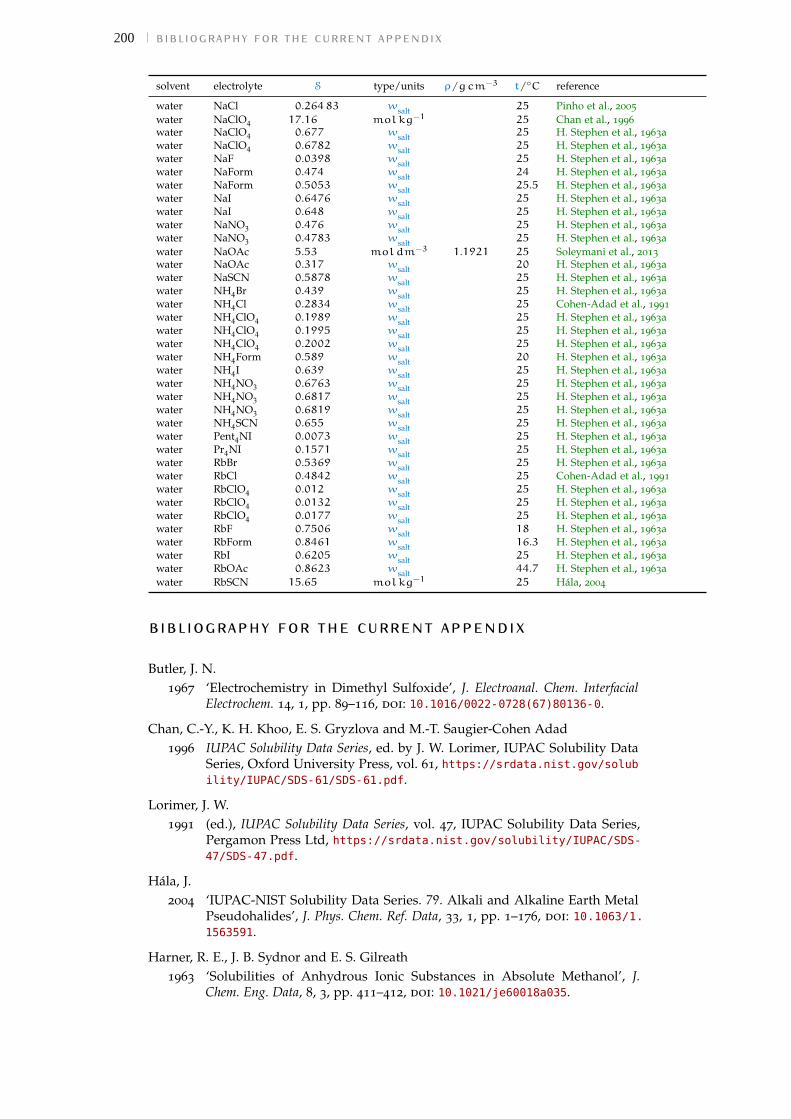
200 bibliography for the current appendix
solvent electrolyte S type/units ρ/gcm−3 t/◦C reference
water NaCl 0.26483 wsalt 25 Pinho et al., 2005water NaClO4 17.16 molkg−1 25 Chan et al., 1996water NaClO4 0.677 wsalt 25 H. Stephen et al., 1963awater NaClO4 0.6782 wsalt 25 H. Stephen et al., 1963awater NaF 0.0398 wsalt 25 H. Stephen et al., 1963awater NaForm 0.474 wsalt 24 H. Stephen et al., 1963awater NaForm 0.5053 wsalt 25.5 H. Stephen et al., 1963awater NaI 0.6476 wsalt 25 H. Stephen et al., 1963awater NaI 0.648 wsalt 25 H. Stephen et al., 1963awater NaNO3 0.476 wsalt 25 H. Stephen et al., 1963awater NaNO3 0.4783 wsalt 25 H. Stephen et al., 1963awater NaOAc 5.53 moldm−3 1.1921 25 Soleymani et al., 2013water NaOAc 0.317 wsalt 20 H. Stephen et al., 1963awater NaSCN 0.5878 wsalt 25 H. Stephen et al., 1963awater NH4Br 0.439 wsalt 25 H. Stephen et al., 1963awater NH4Cl 0.2834 wsalt 25 Cohen-Adad et al., 1991water NH4ClO4 0.1989 wsalt 25 H. Stephen et al., 1963awater NH4ClO4 0.1995 wsalt 25 H. Stephen et al., 1963awater NH4ClO4 0.2002 wsalt 25 H. Stephen et al., 1963awater NH4Form 0.589 wsalt 20 H. Stephen et al., 1963awater NH4I 0.639 wsalt 25 H. Stephen et al., 1963awater NH4NO3 0.6763 wsalt 25 H. Stephen et al., 1963awater NH4NO3 0.6817 wsalt 25 H. Stephen et al., 1963awater NH4NO3 0.6819 wsalt 25 H. Stephen et al., 1963awater NH4SCN 0.655 wsalt 25 H. Stephen et al., 1963awater Pent4NI 0.0073 wsalt 25 H. Stephen et al., 1963awater Pr4NI 0.1571 wsalt 25 H. Stephen et al., 1963awater RbBr 0.5369 wsalt 25 H. Stephen et al., 1963awater RbCl 0.4842 wsalt 25 Cohen-Adad et al., 1991water RbClO4 0.012 wsalt 25 H. Stephen et al., 1963awater RbClO4 0.0132 wsalt 25 H. Stephen et al., 1963awater RbClO4 0.0177 wsalt 25 H. Stephen et al., 1963awater RbF 0.7506 wsalt 18 H. Stephen et al., 1963awater RbForm 0.8461 wsalt 16.3 H. Stephen et al., 1963awater RbI 0.6205 wsalt 25 H. Stephen et al., 1963awater RbOAc 0.8623 wsalt 44.7 H. Stephen et al., 1963awater RbSCN 15.65 molkg−1 25 Hála, 2004
bibliography for the current appendixButler, J. N.
1967 ‘Electrochemistry in Dimethyl Sulfoxide’, J. Electroanal. Chem. InterfacialElectrochem. 14, 1, pp. 89–116, doi: 10.1016/0022-0728(67)80136-0.
Chan, C.-Y., K. H. Khoo, E. S. Gryzlova and M.-T. Saugier-Cohen Adad1996 IUPAC Solubility Data Series, ed. by J. W. Lorimer, IUPAC Solubility Data
Series, Oxford University Press, vol. 61, https://srdata.nist.gov/solubility/IUPAC/SDS-61/SDS-61.pdf.
Lorimer, J. W.1991 (ed.), IUPAC Solubility Data Series, vol. 47, IUPAC Solubility Data Series,
Pergamon Press Ltd, https://srdata.nist.gov/solubility/IUPAC/SDS-47/SDS-47.pdf.
Hála, J.2004 ‘IUPAC-NIST Solubility Data Series. 79. Alkali and Alkaline Earth Metal
Pseudohalides’, J. Phys. Chem. Ref. Data, 33, 1, pp. 1–176, doi: 10.1063/1.1563591.
Harner, R. E., J. B. Sydnor and E. S. Gilreath1963 ‘Solubilities of Anhydrous Ionic Substances in Absolute Methanol’, J.
Chem. Eng. Data, 8, 3, pp. 411–412, doi: 10.1021/je60018a035.
bibliography for the current appendix 201
Harris, W. S.1958 Electrochemical Studies in Cyclic Esters, PhD thesis, California Univ., Berke-
ley, CA (US). Radiation Lab., doi: 10.2172/4305596.
Hernández-Luis, F., R. Rodríguez-Raposo, H. R. Galleguillos and J. W. Morales2016 ‘Solubility of Sodium Halides in Aqueous Mixtures with ε-increasing
Cosolvents: Formamide, N-methylformamide, and N-methylacetamide at298.15K’, Ind. Eng. Chem. Res. 55, 3, pp. 812–819, doi: 10.1021/acs.iecr.5b04614.
Labban, A.-K. S. and Y. Marcus1991 ‘The Solubility and Solvation of Salts in Mixed Nonaqueous Solvents. 1.
Potassium Halides in Mixed Aprotic Solvents’, J. Solution Chem. 20, 2,pp. 221–232, doi: 10.1007/BF00649530.
1997 ‘The Solubility and Solvation of Salts in Mixed Nonaqueous Solvents. 2.Potassium Halides in Mixed Protic Solvents’, J. Solution Chem. 26, 1, pp. 1–12, doi: 10.1007/BF02439440.
Li, M., D. Constantinescu, L. Wang, A. Mohs and J. Gmehling2010 ‘Solubilities of NaCl, KCl, LiCl, and LiBr in Methanol, Ethanol, Acetone,
and Mixed Solvents and Correlation Using the LIQUAC Model’, Ind. Eng.Chem. Res. 49, 10, pp. 4981–4988, doi: 10.1021/ie100027c.
Muhuri, P. K., S. K. Ghosh and D. K. Hazra1993 ‘Solubilities of Some Alkali-metal Salts, Tetraphenylarsonium Chloride,
and Tetraphenylphosphonium Bromide in Propylene Carbonate at 25 ◦CUsing the Ion-selective Electrode Technique’, J. Chem. Eng. Data, 38, 2,pp. 242–244, doi: 10.1021/je00010a014.
Peruzzi, N., P. Lo Nostro, B. W. Ninham and P. Baglioni2015 ‘The Solvation of Anions in Propylene Carbonate’, J. Solution Chem. 44 (6
2015), pp. 1224–1239, doi: 10.1007/s10953-015-0335-z.
Peruzzi, N., B. W. Ninham, P. Lo Nostro and P. Baglioni2012 ‘Hofmeister Phenomena in Nonaqueous Media: The Solubility of Electro-
lytes in Ethylene Carbonate’, J. Phys. Chem. B, 116, 49, pp. 14398–14405,doi: 10.1021/jp309157x.
Pinho, S. P. and E. A. Macedo2005 ‘Solubility of NaCl, NaBr, and KCl in Water, Methanol, Ethanol, and Their
Mixed Solvents’, J. Chem. Eng. Data, 50, 1, pp. 29–32, doi: 10.1021/je049922y.
Scrosati, B. and C. A. Vincent1980 Alkali Metal, Alkaline Earth Metal and Ammonium Halides, Amide Solvents, ed.
by A. S. Kertes, IUPAC Solubility Data Series, Pergamon Press Ltd, vol. 11,https://srdata.nist.gov/solubility/IUPAC/SDS-11/SDS-11.pdf.
Soleymani, J., M. Zamani-Kalajahi, B. Ghasemi, E. Kenndler and A. Jouyban2013 ‘Solubility of Sodium Acetate in Binary Mixtures of Methanol, 1-propanol,
Acetonitrile, and Water at 298.2K’, J. Chem. Eng. Data, 58, 12, pp. 3399–3404, doi: 10.1021/je400625f.
Stenger, V. A.1996 ‘Solubilities of Various Alkali Metal and Alkaline Earth Metal Compounds
in Methanol’, J. Chem. Eng. Data, 41, 5, pp. 1111–1113, doi: 10.1021/je960124k.
Stephen, H. and T. Stephen1963a (eds.), Solubilities of Inorganic and Organic Compounds. Binary Systems,
vol. 1.1, Pergamon Press, Oxford.

202 bibliography for the current appendix
Stephen, H. and T. Stephen1963b (eds.), Solubilities of Inorganic and Organic Compounds. Binary Systems,
vol. 1.2, Pergamon Press, Oxford.
Turner, W. E. S. and C. C. Bissett1913 ‘CCIV.— The Solubilities of Alkali Haloids in Methyl, Ethyl, Propyl, and
isoamyl Alcohols’, J. Chem. Soc., Trans. 103 (0 1913), pp. 1904–1910, doi:10.1039/CT9130301904.

E C U S TO M C O N D U C T I V I T Y C E L L1 1
2 2
3 3
4 4
5 5
6 6
AA
BB
CC
DD
SH
EET 1 O
F 1
DESIG
NED
:
9/11/2017
CO
MPO
NEN
T:
TITLE
SIZE
A3
SCALE
REV
AP
PLIE
D M
AT
HE
MA
TIC
S D
EP
AR
TM
EN
T A
.N
.U
To
le
ra
nce
s (u
nle
ss o
th
erw
ise
sta
te
d)
0 +
-0
.2
5
0.0
+
-0
.1
0
0.0
0 +
-0
.0
5
SU
RF
AC
E FIN
IS
H:
1.6
um
A
LL O
VE
R U
NL
ES
S S
TA
TE
D O
TH
ER
WIS
E
UN
IT Q
TY
Ron Cruikshank
DRAW
N: R
on Cruikshank
DO
N
OT SCALE
As N
oted
4.
0
0
5.02
Figu
re92
:Sch
emat
ics
ofth
ecu
stom
-mad
eco
nduc
tivi
tyce
llbo
dy,
empl
oyed
asth
ede
tect
orin
the
sec
expe
ri-
men
ts.
Dra
win
gcr
edit
s:M
r.R
onC
ruik
shan
k,D
epar
tmen
tof
App
lied
Mat
hem
atic
s,R
esea
rch
Scho
olof
Phys
ics
and
Engi
neer
ing,
AN
U.
203


F E F F E C T O F W AT E R I M P U R I T I E SO N SEC A N D QCM E X P E R I M E N T S
In this section, I present and discuss some experiments I performed in order toascertain the impact of water contamination on the sie trends for sec and qcmexperiments in non-aqueous solvents.
f.1 Size-exclusion chromatographyIn meoh, the sec runs of NaF, NaCl and NaBr, when a small amount of wa-
ter is added to either the sample or the eluent, are compared. Figure 93 showschromatograms of repeat runs where the water content in the sample or the elu-ent is approximately doubled. No significant effect is seen on the position of thepeak after doubling the water content in the eluent or sample. This suggests thatthe results we observe are largely unaffected by the presence of small quantities ofwater.In contrast, the NaI sample peak in pc has a different shape in the final anhydrousruns with respect to the trial ones (Fig. 94). The trial runs were performed in non-anhydrous eluent, wwater% ≈ 0.04 for the solvent in the bottle, but the column wasnot sealed from moisture, so a much higher water content was present in these trialruns. In the anhydrous runs, the water content of the NaI sample iswwater% = 0.015.In the non-anhydrous trial case the NaI sample is eluting sharply (also notice thatNaBr is behaving as ‘sticky’—NaBr has not been tested in the final anhydrous runsdue to low solubility), whereas in anhydrous conditions NaI sticks to the stationaryphase.In order to understand the origin of this difference, the anhydrous run of Fig. 24was repeated for confirmation, and then another run was performed with a NaIsample containing a higher water content. This sample was prepared by addingwater to the NaI anhydrous sample (wwater% = 0.015), and it had a water content of1.3% (measured by kf). The three runs at different sample water content are shownin Fig. 95: no difference in the peak shape is observed.This evidence in pc indicates that the behaviour of ions can indeed change based onthe water content in the non-aqueous aprotic solvent, but to induce such a change,the water content needs to be high, as in the trial experiments. This is interestingbecause it suggests that the amount of water in solution can modulate the behaviourof anions in non-aqueous solvents. This agrees with the rule of thumb proposedin Chapter 4: the ordering of anions in water and non-aqueous aprotic solventsis likely to be different. It is also in accordance with the literature evidence ofpreferential solvation of anions in aprotic solvents.However, in dmso no changes in the peak shape or elution order have been noticedbetween the non-anhydrous trial runs and the final anhydrous runs (Fig. 96). It ispossible that the water content has to be higher in order to affect the behaviour of
205

206 effect of water impurities on sec and qcm experiments
NaF NaCl NaBr
0 50 100 150 200 0 50 100 150 200 0 50 100 150 200
0.0
0.2
0.4
0.6
0.8
0.00
0.25
0.50
0.75
1.00
0.00
0.05
0.10
0.15
elution volume / ml
rela
tive
cond
ucti
vity
0.10.20.30.40.5
wsampleH2O %
(a) NaF, NaCl and NaBr samples with differing water concentrations.
NaF NaCl NaBr
0 50 100 150 200 0 50 100 150 200 0 50 100 150 200
0.0
0.2
0.4
0.6
0.8
0.00
0.25
0.50
0.75
1.00
0.00
0.05
0.10
0.15
elution volume / ml
rela
tive
cond
ucti
vity
0.04
0.06
0.08
0.10
weluentH2O %
(b) Eluent (meoh) with varying water concentration.
Figure 93: Effect of the addition of water on the sec elution peaks of NaF, NaCl and NaBrin meoh. Water is added to the sample (top) or to the eluent (bottom). Thebaseline conductivity of the pure solvent has been subtracted and the values ofthe conductivity rescaled relative to the maximum conductivity being set to 1.
NaBr 188.4ml
NaI 41.1ml
NaI 60.5ml
trial run (non-anhydrous) anhydrous
0 20 40 60 80 100 120 140 160 180 200 220 240 0 20 40 60 80 100 120 140 160 180
0.0
0.1
0.2
0.3
0.4
0.5
0.6
0.7
0.8
0.9
1.0
elution volume / ml
rela
tive
cond
ucti
vity
Figure 94: Chromatography runs in pc in different water content conditions. The NaBrsample is constituted of a saturated solution. The NaI data plotted on the anhyd-rous panel are the same as in Fig. 24 in Chapter 6. The baseline conductivity ofthe pure solvent has been subtracted and the values of the conductivity rescaledrelative to the maximum conductivity being set to 1.
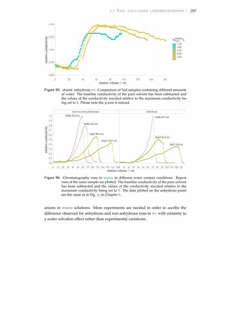
f.1 Size-exclusion chromatography 207
0.000
0.025
0.050
0.075
0.100
0 20 40 60 80 100 120 140 160
elution volume / ml
rela
tive
cond
ucti
vity
0.250.500.751.001.25
wsampleH2O %
Figure 95: eluent: anhydrous pc. Comparison of NaI samples containing different amountsof water. The baseline conductivity of the pure solvent has been subtracted andthe values of the conductivity rescaled relative to the maximum conductivity be-ing set to 1. Please note the y-axis is resized.
NaBr 56.4ml
NaBr 64.2ml
NaCl 85.3ml
NaCl 114.1ml
NaBr 69.3ml
NaCl 81.9ml
NaCl 120ml
trial run (non-anhydrous) anhydrous
0 10 20 30 40 50 60 70 80 90 100 110 120 1300 10 20 30 40 50 60 70 80 90 100 110 120 130
0.0
0.1
0.2
0.3
0.4
0.5
0.6
0.7
0.8
0.9
1.0
elution volume / ml
rela
tive
cond
ucti
vity
Figure 96: Chromatography runs in dmso in different water content conditions. Repeatruns of the same sample are plotted. The baseline conductivity of the pure solventhas been subtracted and the values of the conductivity rescaled relative to themaximum conductivity being set to 1. The data plotted on the anhydrous panelare the same as in Fig. 23 in Chapter 6.
anions in dmso solutions. More experiments are needed in order to ascribe thedifference observed for anhydrous and non anhydrous runs in pc with certainty toa water solvation effect rather than experimental variations.
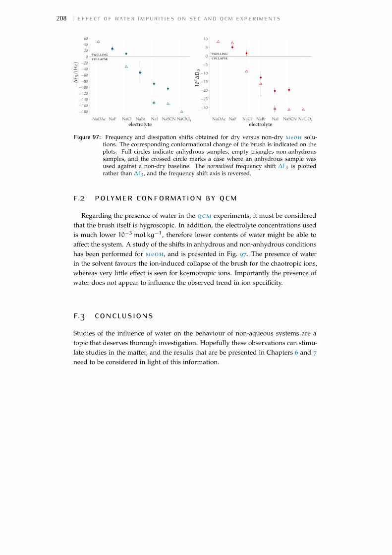
208 effect of water impurities on sec and qcm experiments
collapseswelling
−180
−160
−140
−120
−100
−80
−60
−40
−20
0
20
40
60
NaBrNaCl NaClO4NaF NaINaOAc NaSCNelectrolyte
−∆F3/(Hz)
swellingcollapse
−30
−25
−20
−15
−10
−5
0
5
10
NaBrNaCl NaClO4NaF NaINaOAc NaSCNelectrolyte
106∆D
3
Figure 97: Frequency and dissipation shifts obtained for dry versus non-dry meoh solu-tions. The corresponding conformational change of the brush is indicated on theplots. Full circles indicate anhydrous samples, empty triangles non-anhydroussamples, and the crossed circle marks a case where an anhydrous sample wasused against a non-dry baseline. The normalised frequency shift ∆F3 is plottedrather than ∆f3, and the frequency shift axis is reversed.
f.2 polymer conformation by qcmRegarding the presence of water in the qcm experiments, it must be considered
that the brush itself is hygroscopic. In addition, the electrolyte concentrations usedis much lower 10−3molkg−1, therefore lower contents of water might be able toaffect the system. A study of the shifts in anhydrous and non-anhydrous conditionshas been performed for meoh, and is presented in Fig. 97. The presence of waterin the solvent favours the ion-induced collapse of the brush for the chaotropic ions,whereas very little effect is seen for kosmotropic ions. Importantly the presence ofwater does not appear to influence the observed trend in ion specificity.
f.3 conclusionsStudies of the influence of water on the behaviour of non-aqueous systems are atopic that deserves thorough investigation. Hopefully these observations can stimu-late studies in the matter, and the results that are be presented in Chapters 6 and 7need to be considered in light of this information.

G A S U M M A R Y O F U N S U C C E S S F U LA P P R OA C H E S
This appendix summarises the experimental projects that did not yield positiveresults.
g.1 standard molar volume measurementsAs the experimental standard molar volumes values of a number of non-aqueouselectrolytes are not available in the literature, I attempted to obtain them by measur-ing the density of their solutions, in order to employ the values so-obtained in thecalculations of Chapter 3.I therefore performed measurements of the density of electrolyte solutions in meohwith an Anton-Paar DMA 5000 density-meter. The reason why this experiment wasunsuccessful is that we did not record monotonic trends of density when approach-ing higher dilution.Following is a short briefing about the experimental details that could be useful forrepeating the measurements successfully.
g.1.1 Measurements of partial molar volumes
Partial molar volumes in solution have been introduced in Section 3.2. In the fol-lowing discussion, that details the connection between the solution density and thepartial molar volume of the electrolyte, only binary solutions are considered, andthe solvent is denoted by the subscript ‘1’, whereas the solute by the subscript ‘2’.The apparent molal volume φV2 of the solute in solution is defined as:
φV2 =
V −n1V1∗
n2(T, P constant) [21]
where V1∗ is the partial molar volume of the pure solvent. The meaning of Eq. [21]
is that the apparent molar volume is the molar volume of the solute in the hypo-thetical situation where the solvent has maintained the volume it had as a puresubstance. The apparent molar volumes have little thermodynamic utility, exceptfor their function in the determination of the partial molal quantities. The relation-ship between apparent and partial molar quantities is the following:
V2 =
(∂V
∂n2
)
T, P, n1
=φV2 +n2
(∂φV2
∂n2
)
T, P, n1
[22]
From Eq. [22] it is evident that, at infinite dilution:
limn2→0
V2 ≡ V−◦2 =
φV2 [23]
the apparent molar volume of the solute coincides with its standard partial molarvolume.We now need to express φV2 in terms of the experimental observable, the density ρ ofthe solution. The total volume of the solution is related to its density by:
V =w
ρ=n1M1 +n2M2
ρ
209

210 a summary of unsuccessful approaches
NaCl
NaF
NaOAc
NaBr
NaClO4
NaI
NaSCN
1000
1200
1400
1600
1800
0 5 10 15
m/(molkg−1)
ρ/(kgm
−3)
Figure 98: Concentration dependence of the solution density upon molal concentration forthe investigated electrolytes. Density data from Söhnel and Novotný (1985).
Where w is the mass of the solution and w = w1 +w2 = n1M1 + n2M2. Equa-tion Eq. [21] can therefore be rewritten as:
φV2 =
V −n1V−◦1
n2=1
n2
(n1M1 +n2M2
ρ−n1V
−◦1
)[24]
If we express the concentration in terms of the molality of solute in solution m2
(molkg−1(solvent)), then n2 ≡ m2 and n1 is the number of moles of solvent in 1000 g
of solvent: n1 = 1000/M1; by substituting in Eq. [24] we have:
φV2 =
1000(ρ∗ − ρ)m2ρρ
∗ +M2
ρ[25]
Which expresses the partial molar volume of the solute in terms of the density of thesolution, the density of the pure solvent and the molality of solute. In this equation,the densities are expressed in g cm−3, the molar masses in gmol−1 and the molalityof solute in molkg−1
(solvent), therefore the apparent partial molar volume is obtained
in cm3mol−1 and a factor of 1000 is present.By measuring the densities of electrolyte solutions at several finite concentrations,we can therefore calculate the apparent partial molar volume through Eq. [25], andthen extrapolate the apparent molar volume to infinite dilution, where it coincideswith the standard partial molar volume (Eq. [23]). Figure 98 shows the dependence ofthe density of solutions of the electrolytes of interest upon concentration.
Extrapolation to infinite dilution
In order to obtain the standard partial molar volume V−◦2 of an electrolyte, its appar-
ent molar volume, calculated from the measured densities at finite concentrationby Eq. [25], needs to be extrapolated to infinite dilution. The RRM equation isthe recommended model for the extrapolation (Marcus and Hefter, 2004; Millero,1972b):
φV2 = V
−◦2 + S
dhv√c2 + bvc2
It satisfactorily fits data up to ≈ 1mol dm−3 for the majority of systems. Therefore,
a plot of(φV2 − S
dhv√c2
)versus c2 is usually linear and yields V
−◦2 as intercept
and bv as slope.
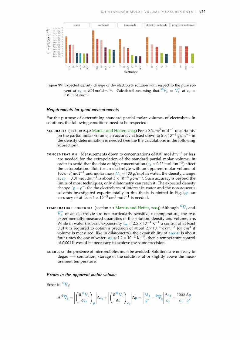
g.1 standard molar volume measurements 211
water methanol formamide dimethyl sulfoxide propylene carbonate
I–
ClO
4–
Br–
F–
AcO
–
Cl–
SCN
– I–
ClO
4–
Br–
SCN
–
Cl–
F– I–
Br–
ClO
4–
Cl–
F–
SCN
– I–
Br–
ClO
4–
Cl–
F– I–
Br–
ClO
4–
Cl–
3.0× 10−44.0× 10−45.0× 10−46.0× 10−47.0× 10−48.0× 10−49.0× 10−41.0× 10−31.1× 10−31.2× 10−31.3× 10−31.4× 10−31.5× 10⁻³
electrolyte
(ρ−ρ∗ )/(gcm
−3)
Figure 99: Expected density change of the electrolyte solution with respect to the pure sol-vent at c2 = 0.01mol dm−3. Calculated assuming that φV2 ≈ V
−◦2 at c2 =
0.01mol dm−3.
Requirements for good measurements
For the purpose of determining standard partial molar volumes of electrolytes insolutions, the following conditions need to be respected:
accuracy: (section 2.4.2 Marcus and Hefter, 2004) For a 0.5 cm3mol−1 uncertaintyon the partial molar volume, an accuracy at least down to 5× 10⁻⁶ g cm−3 inthe density determination is needed (see the the calculations in the followingsubsection).
concentration: Measurements down to concentrations of 0.01mol dm−3 or lessare needed for the extrapolation of the standard partial molar volume, inorder to avoid that the data at high concentration (c2 > 0.25mol dm−3) affectthe extrapolation. But, for an electrolyte with an apparent molar volume of100 cm3mol−1 and molar mass Mi = 100 g/mol in water, the density changeat c2 = 0.01mol dm−3 is about 3× 10⁻⁶ g cm−3. Such accuracy is beyond thelimits of most techniques, only dilatometry can reach it. The expected densitychange (ρ − ρ∗) for the electrolytes of interest in water and the non-aqueoussolvents investigated experimentally in this thesis is plotted in Fig. 99: anaccuracy of at least 1× 10⁻⁵ cm3mol−1 is needed.
temperature control: (section 2.1 Marcus and Hefter, 2004) Although φV2 andV−◦2 of an electrolyte are not particularly sensitive to temperature, the two
experimentally measured quantities of the solution, density and volume, are.While in water (isobaric expansivity αp ≈ 2.5× 10⁻⁴ K−1 a control of at least0.01K is required to obtain a precision of about 2× 10⁻⁶ g cm−3 (or cm3 ifvolume is measured, like in dilatometry), the expansibility of meoh is aboutfour times the one of water: αp ≈ 1.2× 10⁻³ K−1), then a temperature controlof 0.001K would be necessary to achieve the same precision.
bubbles: the presence of microbubbles must be avoided. Solutions are not easy todegas =⇒ sonication; storage of the solutions at or slightly above the meas-urement temperature.
Errors in the apparent molar volume
Error in φV2:
∆φV2 =
∣∣∣∣∣
(∂φV2
∂c2
)
ρ
∣∣∣∣∣∆c2 +
∣∣∣∣∣
(∂φV2∂ρ
)
c2
∣∣∣∣∣∆ρ =
∣∣∣∣∣M2
ρ∗−φV2
∣∣∣∣∣∆c2
c2+1000
c2
∆ρ
ρ∗

212 a summary of unsuccessful approaches
In dilute solutions the apparent molar volume is not seriously influenced by errorson c2, but it is largely affected by errors in ρ: in water, if c2 = 0.01mol dm−3, a5× 10−6 g cm−3 error in ρ causes an error of c2 = 0.5 cm3mol−1 in ∆φV2.
g.2 turbidimetryThis work was aimed at investigating the stability of colloids in non-aqueous sol-vents in the presence of different electrolytes.We tested Boehmite nanopowders (Sasol Disperal). These powders are water or aciddispersible, and I tried dispersing them in non-aqueous solvents. I found that Dis-peral D40 formed stable suspensions in neat meoh and Disperal P2W was stable inneat fa and pc . All the suspensions were stable for longer than 20 d.I then suspended the powders in solutions of the electrolytes in the solvents andmonitored the sedimentation kinetics by means of a turbidimeter. Although the pre-liminary measurements where promising and I thought I was measuring a depend-ence of the sedimentation kinetics upon the electrolyte present, after repeated runsI realised that the variability in the sedimentation process was very high, renderingthe averaged sedimentation curves for different electrolytes undistinguishable.Therefore, the decrease in turbidity with time does not seem to be due to salt-specific aggregation and sedimentation.
g.3 Nmr T2 relaxation times of salt solutionsNmr can be used to investigate solvation processes. The transversal relaxation timeT2 is sensitive to relaxation phenomena within the sample. It is therefore useful toinvestigate effects of a solute on the relaxation of the solvent molecules.We performed measurements on samples made of the seven electrolytes and thefour solvents that are the object of the investigating experimental investigations ofthis thesis, with a benchtop nmr instrument: the Acorn Area from Xigo Nanotools.We found that the instrument showed variations in the data readings that were notcorrelated to environmental effects. We later also understood that the magnitudeof the effects that we intended to measure are beyond the instrument accuracy, andtherefore this project was abandoned.
g.4 swelling of commercial hydrogelsI have also attempted to monitor the swelling of commercial hydrogels beads in thepresence of non-aqueous electrolytes solutions.On preliminary testing, I found out that the beads would only swell in water andfa, and therefore excluded the other solvents.I monitored the changes in mass of the bead after being equilibrated in a salt solu-tion with respect to the pure solvent. An overall shrinking trend in the presenceof the salt solution was observed, which was promising. But the bead would oftenbreak as a consequence of handling. In addition, the weight loss in presence of theelectrolytes was very similar across the four salts tested. Also this experiment wasabandoned.

B I B L I O G R A P H Y
Andrieu-Brunsen, A., S. Micoureau, M. Tagliazucchi, I. Szleifer, O. Azzaroniand G. J. A. A. Soler-Illia
2015 ‘Mesoporous Hybrid Thin Film Membranes with PMETAC@silicaArchitectures: Controlling Ionic Gating through the Tuning of Poly-electrolyte Density’, Chem. Mater. 27, 3, pp. 808–821, doi: 10.1021/cm5037953.
Ao, Z., G. Liu and G. Zhang2011 ‘Ion Specificity at Low Salt Concentrations Investigated with Total
Internal Reflection Microscopy’, J. Phys. Chem. C, 115, 5, pp. 2284–2289, doi: 10.1021/jp110782g.
Aoki, K., K. Shiraki and T. Hattori2016 ‘Salt Effects on the Picosecond Dynamics of Lysozyme Hydration
Water Investigated by Terahertz Time-domain Spectroscopy and anInsight into the Hofmeister Series for Protein Stability and Solubil-ity’, Phys. Chem. Chem. Phys. 18, 22, pp. 15060–15069, doi: 10.1039/c5cp06324h.
Arakawa, T. and S. N. Timasheff1984 ‘Mechanism of Protein Salting in and Salting Out by Divalent
Cation Salts: Balance between Hydration and Salt Binding’, Biochem-istry, 23, 25, pp. 5912–5923, doi: 10.1021/bi00320a004.
Armarego, W. L. F. and C. L. L. Chai2009 Purification of Laboratory Chemicals, 6th ed., Butterworth-Heinemann,
Burlington, MA.
Arslanargin, A., A. Powers, T. L. Beck and S. W. Rick2016 ‘Models of Ion Solvation Thermodynamics in Ethylene Carbonate
and Propylene Carbonate’, J. Phys. Chem. B, 120, 8, pp. 1497–1508,doi: 10.1021/acs.jpcb.5b06891.
Asthagiri, D., M. R. Schure and A. M. Lenhoff2000 ‘Calculation of Hydration Effects in the Binding of Anionic Ligands
to Basic Proteins’, J. Phys. Chem. B, 104, 36, pp. 8753–8761, doi: 10.1021/jp001458q.
Aurbach, D., Y. Talyosef, B. Markovsky, E. Markevich, E. Zinigrad, L. Asraf,J. S. Gnanaraj and H.-J. Kim
2004 ‘Design of Electrolyte Solutions for Li and Li-ion Batteries: A Re-view’, Electrochim. Acta, 50, 2-3, pp. 247–254, doi: 10 . 1016 / j .
electacta.2004.01.090.
Ayres, N.2010 ‘Polymer Brushes: Applications in Biomaterials and Nanotechno-
logy’, Polym. Chem. 1 (6 2010), pp. 769–777, doi: 10.1039/B9PY00246D.
213

214 bibliography
Azzaroni, O., S. Moya, T. Farhan, A. A. Brown and W. T. S. Huck2005 ‘Switching the Properties of Polyelectrolyte Brushes Via “Hydro-
phobic Collapse”’, Macromolecules, 38, 24, pp. 10192–10199, doi: 10.1021/ma051549r.
Baldwin, R. L.1996 ‘How Hofmeister Ion Interactions Affect Protein Stability’, Biophys.
J. 71, 4, pp. 2056–2063, doi: 10.1016/S0006-3495(96)79404-3.
Barthel, J., R. Neueder and G. Lauermann1985 ‘Vapor Pressures of Non-aqueous Electrolyte Solutions. Part 1. Al-
kali Metal Salts in Methanol’, J. Solution Chem. 14, 9, pp. 621–633,doi: 10.1007/BF00646055.
Barthel, J., R. Neueder and H. Roch2000 ‘Density, Relative Permittivity, and Viscosity of Propylene Carbon-
ate + Dimethoxyethane Mixtures from 25 ◦C to 125 ◦C’, J. Chem. Eng.Data, 45, 6, pp. 1007–1011, doi: 10.1021/je000098x.
Batoulis, H., T. H. Schmidt, P. Weber, J.-G. Schloetel, C. Kandt and T. Lang2016 ‘Concentration Dependent Ion-protein Interaction Patterns Un-
derlying Protein Oligomerization Behaviours’, Sci. Rep. 6, 24131,p. 24131, doi: 10.1038/srep24131.
Beck, T. L.2011 ‘A Local Entropic Signature of Specific Ion Hydration’, J. Phys.
Chem. B, 115, 32, pp. 9776–9781, doi: 10.1021/jp204883h.
Béguin, F., V. Presser, A. Balducci and E. Frackowiak2014 ‘Carbons and Electrolytes for Advanced Supercapacitors’, Adv. Ma-
ter. 26, 14, pp. 2219–2251, doi: 10.1002/adma.201304137.
Biesalski, M., D. Johannsmann and J. Rühe2004 ‘Electrolyte-induced Collapse of a Polyelectrolyte Brush’, J. Chem.
Phys. 120, 18, pp. 8807–8814, doi: 10.1063/1.1690242.
Bilanicová, D., A. Salis, B. W. Ninham and M. Monduzzi2008 ‘Specific Anion Effects on Enzymatic Activity in Nonaqueous Me-
dia’, J. Phys. Chem. B, 112, 38, pp. 12066–12072, doi: 10 . 1021 /
jp805451w.
Bjørnsdottir, I., J. Tjørnelund and S. H. Hansen1998 ‘Nonaqueous Capillary Electrophoresis — Its Applicability in the
Analysis of Food, Pharmaceuticals and Biological Fluids’, Electro-phoresis, 19, 12, pp. 2179–86, doi: 10.1002/elps.1150191223.
Böes, E. S., P. R. Livotto and H. Stassen2006 ‘Solvation of Monovalent Anions in Acetonitrile and N,N-
dimethylformamide: Parameterization of the IEF-PCM Model’,Chem. Phys. 331, 1, pp. 142–158, doi: 10.1016/j.chemphys.2006.08.028.
Bosque, R. and J. Sales2002 ‘Polarizabilities of Solvents from the Chemical Composition’, J.
Chem. Inf. Comput. Sci. 42, 5, pp. 1154–1163, doi: 10.1021/ci025528x.
bibliography 215
Boström, M., F. W. Tavares, S. Finet, F. Skouri-Panet, A. Tardieu and B. W.Ninham
2005 ‘Why Forces between Proteins Follow Different Hofmeister Seriesfor pH above and below pI’, Biophys. Chem. 117, 3, pp. 217–224, doi:10.1016/j.bpc.2005.05.010.
Breslow, R. and T. Guo1988 ‘Diels-Alder Reactions in Nonaqueous Polar Solvents. Kinetic
Effects of Chaotropic and Antichaotropic Agents and of β-cyclodextrin’, J. Am. Chem. Soc. 110, 17, pp. 5613–5617, doi: 10.1021/ja00225a003.
Bromley, L. A.1973 ‘Thermodynamic Properties of Strong Electrolytes in Aqueous Solu-
tions’, AIChE J. 19, 2, pp. 313–320, doi: 10.1002/aic.690190216.
Bruttel, P. and R. Schlink2006 Water Determination by Karl Fischer Titration, Metrohm Monograph,
Metrohm Ltd., Switzerland, http://metrohmsiam.com/foodlab/FL_38/Monograph_WaterDeterminationKF.pdf.
Butler, J. N.1967 ‘Electrochemistry in Dimethyl Sulfoxide’, J. Electroanal. Chem. Inter-
facial Electrochem. 14, 1, pp. 89–116, doi: 10.1016/0022-0728(67)80136-0.
Butler, J. N., D. R. Cogley and E. Grunwald1971 ‘Selective Solvation of Ions by Water in Propylene Carbonate’, J.
Phys. Chem. 75, 10, pp. 1477–1486, doi: 10.1021/j100680a018.
Butler, R. N. and M. C. R. Symons1969 ‘Solvation Spectra. Part 29. Nuclear Magnetic Resonance Studies
of Electrolyte Solutions : Ion-solvent Interactions in Methanol’, en,Trans. Faraday Soc. 65, pp. 2559–2566, doi: 10.1039/tf9696502559.
Cacace, M. G., E. M. Landau and J. J. Ramsden1997 ‘The Hofmeister Series: Salt and Solvent Effects on Interfacial
Phenomena’, Q. Rev. Biophys. 30, 03, pp. 241–277, doi: 10 . 1017 /
S0033583597003363.
Calligaris, S. and M. C. Nicoli2006 ‘Effect of Selected Ions from Lyotropic Series on Lipid Oxidation
Rate’, Food Chem. 94, 1, pp. 130–134, doi: 10.1016/j.foodchem.2004.11.002.
Carpenter, D. C. and F. E. Lovelace1935 ‘The Influence of Neutral Salts on the Optical Rotation of Gela-
tin. III. Effect of the Halides of Lithium, Sodium, Rubidium andCesium’, J. Am. Chem. Soc. 57, 12, pp. 2337–2342, doi: 10 . 1021 /
ja01315a001.
Chan, C.-Y., K. H. Khoo, E. S. Gryzlova and M.-T. Saugier-Cohen Adad1996 IUPAC Solubility Data Series, ed. by J. W. Lorimer, IUPAC Solubility
Data Series, Oxford University Press, vol. 61, https://srdata.nist.gov/solubility/IUPAC/SDS-61/SDS-61.pdf.
216 bibliography
ChemAxon2017 Marvinsketch 17.27.0, www.chemaxon.com/products/marvin/marvinsket
ch/.
Chen, R., D. Xu, G. Guo and L. Gui2003 ‘Preparation of Ag2Se and Ag2Se1 – xTex Nanowires by Electrode-
position from DMSO Baths’, Electrochem. Commun. 5, 7, pp. 579–583,doi: 10.1016/S1388-2481(03)00133-4.
Chernyak, Y.2006 ‘Dielectric Constant, Dipole Moment, and Solubility Parameters of
Some Cyclic Acid Esters’, J. Chem. Eng. Data, 51, 2, pp. 416–418, doi:10.1021/je050341y.
Chu, X., J. Yang, G. Liu and J. Zhao2014 ‘Swelling Enhancement of Polyelectrolyte Brushes Induced by Ex-
ternal Ions’, Soft Matter, 10 (30 2014), pp. 5568–5578, doi: 10.1039/C4SM00860J.
Collins, K. D.1997 ‘Charge Density-dependent Strength of Hydration and Biological
Structure’, Biophys. J. 72, 1, pp. 65–76, doi: 10.1016/S0006-3495(97)78647-8.
2004 ‘Ions from the Hofmeister Series and Osmolytes: Effects on Proteinsin Solution and in the Crystallization Process’, Methods, 34, 3, Mac-romolecular Crystallization, pp. 300–311, doi: 10.1016/j.ymeth.2004.03.021.
2006 ‘Ion Hydration: Implications for Cellular Function, Polyelectrolytes,and Protein Crystallization’, Biophys. Chem. 119, 3, pp. 271–281, doi:10.1016/j.bpc.2005.08.010.
2012 ‘Why Continuum Electrostatics Theories Cannot Explain BiologicalStructure, Polyelectrolytes or Ionic Strength Effects in Ion-proteinInteractions’, Biophys. Chem. 167, pp. 43–59, doi: 10.1016/j.bpc.
2012.04.002.
Collins, K. D., G. W. Neilson and J. E. Enderby2007 ‘Ions in Water: Characterizing the Forces That Control Chemical
Processes and Biological Structure’, Biophys. Chem. 128, 2–3, pp. 95–104, doi: 10.1016/j.bpc.2007.03.009.
Collins, K. D. and M. W. Washabaugh1985 ‘The Hofmeister Effect and the Behaviour of Water at Interfaces’, Q.
Rev. Biophys. 18, 4, pp. 323–422, doi: 10.1017/S0033583500005369.
Compu Phase2015 Termite: A Simple RS232 Terminal, www.compuphase.com/software_term
ite.htm.
Conway, B. E.1977 ‘Significance of a Volcano Relation of Fajans for Hydration Ener-
gies’, J. Solution Chem. 6, 1, pp. 23–31, doi: 10.1007/BF00650789.1987 ‘Electrochemical Proton Transfer and Cathodic Hydrogen Evolu-
tion’, Science Progress (1933- ), 71, 4 (284), pp. 479–509, http://www.jstor.org/stable/43420696.
bibliography 217
Cox, W. M. and J. H. Wolfenden1934 ‘The Viscosity of Strong Electrolytes Measured by a Differential
Method’, Proc. R. Soc. A, 145, 855, pp. 475–488, doi: 10.1098/rspa.1934.0113.
Craig, V. S. J., B. W. Ninham and R. M. Pashley1993a ‘Effect of Electrolytes on Bubble Coalescence’, Nature, 364, 6435,
pp. 317–319, doi: 10.1038/364317a0.1993b ‘The Effect of Electrolytes on Bubble Coalescence in Water’, J. Phys.
Chem. 97, 39, pp. 10192–10197, doi: 10.1021/j100141a047.
Craig, V. S. J. and M. Plunkett2003 ‘Determination of Coupled Solvent Mass in Quartz Crystal Mi-
crobalance Measurements Using Deuterated Solvents’, J. Colloid In-terface Sci. 262, 1, pp. 126–129, doi: 10.1016/s0021-9797(03)00210-8.
Crawford, M.-J. and T. M. Klapötke1999 ‘The Synthesis of Tetraphenylarsonium Azide, [Ph4As]+[N3]– , and
the Attempted Preparation of Tetraphenylarsonium Azidodithiocar-bonate, [Ph4As]+[SCSN3]– ’, Heteroat. Chem. 10, 4, pp. 325–329, doi:10.1002/(SICI)1098-1071(1999)10:4<325::AID-HC11>3.0.CO;2-H.
Criss, C. M. and M. J. Mastroianni1971 ‘Some Observations on the Viscosity Coefficients of Ions in Various
Solvents’, J. Phys. Chem. 75, 16, pp. 2532–2534, doi: 10.1021/j100685a022.
DePhillips, P. and A. M. Lenhoff2001 ‘Determinants of Protein Retention Characteristics on Cation-
exchange Adsorbents’, J. Chromatogr. A, 933, 1, pp. 57–72, doi: 10.1016/S0021-9673(01)01275-4.
Desnoyers, J. E., R. E. Verrall and B. E. Conway1965 ‘Electrostriction in Aqueous Solutions of Electrolytes’, J. Chem. Phys.
43, 1, pp. 243–250, doi: 10.1063/1.1696464.
dos Santos, A. P., A. Diehl and Y. Levin2010 ‘Surface Tensions, Surface Potentials, and the Hofmeister Series of
Electrolyte Solutions’, Langmuir, 26, 13, pp. 10778–10783, doi: 10.
1021/la100604k.
Duignan, T. T., M. D. Baer and C. J. Mundy2016 ‘Ions Interacting in Solution: Moving from Intrinsic to Collective
Properties’, Curr. Opin. Colloid Interface Sci. 23, pp. 58–65, doi: 10.1016/j.cocis.2016.05.009.
Duignan, T. T., M. D. Baer, G. K. Schenter and C. J. Mundy2017a ‘Electrostatic Solvation Free Energies of Charged Hard Spheres Us-
ing Molecular Dynamics with Density Functional Theory Interac-tions’, J. Chem. Phys. 147, 16, p. 161716, doi: 10.1063/1.4994912.
Duignan, T. T., M. D. Baer, G. K. Schenter and C. J. Mundy2017b ‘Real Single Ion Solvation Free Energies with Quantum Mechanical
Simulation’, Chem. Sci. 8 (9 2017), pp. 6131–6140, doi: 10.1039/C7SC02138K.
218 bibliography
Duignan, T. T., D. F. Parsons and B. W. Ninham2013a ‘A Continuum Model of Solvation Energies Including Electrostatic,
Dispersion, and Cavity Contributions’, J. Phys. Chem. B, 117, 32,pp. 9421–9429, doi: 10.1021/jp403596c.
2013b ‘A Continuum Solvent Model of the Multipolar Dispersion Solva-tion Energy’, J. Phys. Chem. B, 117, 32, pp. 9412–9420, doi: 10.1021/jp403595x.
2014a ‘A Continuum Solvent Model of Ion-ion Interactions in Water’, Phys.Chem. Chem. Phys. 16 (40 2014), pp. 22014–22027, doi: 10.1039/C4CP02822H.
2014b ‘A Continuum Solvent Model of the Partial Molar Volumes andEntropies of Ionic Solvation’, J. Phys. Chem. B, 118, 11, pp. 3122–3132, doi: 10.1021/jp410956m.
2014c ‘Collins’s Rule, Hofmeister Effects and Ionic Dispersion Interac-tions’, eng, Chem. Phys. Lett. 608, Complete, pp. 55–59, doi: 10.1016/j.cplett.2014.05.056.
Dzubiella, J., M. Fyta, D. Horinek, I. Kalcher, R. R. Netz and N. Schwierz2009 ‘Ion-specificity: From Solvation Thermodynamics to Molecular Sim-
ulations and Back’, in Specific Ion Effects, ed. by W. Kunz, pp. 231–265.
Easteal, A. J. and L. A. Woolf1985 ‘Self-diffusion and Volumetric Measurements for N-
Methylformamide and N,N-Dimethylformamide at Temper-atures from 240K to 313K and Pressures up to 300MPa’, J.Chem. Soc., Faraday Trans. 1, 81 (11 1985), pp. 2821–2833, doi:10.1039/F19858102821.
1988 ‘(p, Vm, T , x) Measurements for (1− x)H2O + xCH3CN in the Range278K to 323K and 0.1MPa to 280MPa I. Experimental Results, Iso-thermal Compressibilities, Isobaric Expansivities, and Partial MolarVolumes’, J. Chem. Thermodyn. 20, 6, pp. 693–699, doi: 10.1016/0021-9614(88)90020-1.
Edmondson, S., V. L. Osborne and W. T. S. Huck2004 ‘Polymer Brushes via Surface-initiated Polymerizations’, Chem. Soc.
Rev. 33 (1 2004), pp. 14–22, doi: 10.1039/B210143M.
Fajans, K.1921 ‘Löslichkeit Und Ionisation Vom Standpunkte Der Atomstruktur’,
Naturwissenschaften, 9, 37, pp. 729–738, doi: 10.1007/BF01487182.
Fajans, K. and G. Karagunis1930 ‘Osmotisches Verhalten Von Starken Elektrolyten in Lösung Und
Hydratation Ihrer Ionen’, Angew. Chem. 43, 48, pp. 1046–1048, doi:10.1002/ange.19300434804.
Fajans, K. and O. Johnson1942 ‘Ion-solvent Interaction and Individual Properties of Electrolytes’, J.
Electrochem. Soc. 82, 1, pp. 273–287, doi: 10.1149/1.3071414.
bibliography 219
Fennell, C. J., A. Bizjak, V. Vlachy and K. A. Dill2009 ‘Ion Pairing in Molecular Simulations of Aqueous Alkali Halide
Solutions’, J. Phys. Chem. B, 113, 19, pp. 6782–6791, doi: 10.1021/
jp809782z.
Fischer, M. H. and G. Moore1907 ‘On the Swelling of Fibrin’, Am. J. Physiol. — Leg. Content, 20, 2,
pp. 330–342, http://ajplegacy.physiology.org/content/20/2/330.short.
Fox, J. M., K. Kang, W. Sherman, A. Héroux, G. M. Sastry, M. Baghbanzadeh,M. R. Lockett and G. M. Whitesides
2015 ‘Interactions between Hofmeister Anions and the Binding Pocket ofa Protein’, J. Am. Chem. Soc. 137, 11, pp. 3859–3866, doi: 10.1021/jacs.5b00187.
Franks, G. V.2002 ‘Zeta Potentials and Yield Stresses of Silica Suspensions in Con-
centrated Monovalent Electrolytes: Isoelectric Point Shift and Ad-ditional Attraction’, J. Colloid Interface Sci. 249, 1, pp. 44–51, doi:10.1006/jcis.2002.8250.
Franks, G. V., S. B. Johnson, P. J. Scales, D. V. Boger and T. W. Healy1999 ‘Ion-specific Strength of Attractive Particle Networks’, Langmuir, 15,
13, pp. 4411–4420, doi: 10.1021/la9815345.
Fridovich, I.1963 ‘Inhibition of Acetoacetic Decarboxylase by Anions. The Hofmeister
Lyotropic Series’, J. Biol. Chem. 238, 2, pp. 592–598, www.jbc.org/
content/238/2/592.full.pdf.
Friedman, R.2013 ‘Electrolyte Solutions and Specific Ion Effects on Interfaces’, J. Chem.
Educ. 90, 8, pp. 1018–1023, doi: 10.1021/ed4000525.
Fulop, G. F. and R. M. Taylor1985 ‘Electrodeposition of Semiconductors’, en, Annu. Rev. Mater. Sci. 15,
1, pp. 197–210, doi: 10.1146/annurev.ms.15.080185.001213.
Funkner, S., G. Niehues, D. A. Schmidt, M. Heyden, G. Schwaab, K. M. Cal-lahan, D. J. Tobias and M. Havenith
2012 ‘Watching the Low-frequency Motions in Aqueous Salt Solutions:The Terahertz Vibrational Signatures of Hydrated Ions’, J. Am. Chem.Soc. 134, 2, pp. 1030–1035, doi: 10.1021/ja207929u.
Gao, Y. Q.2011 ‘Simple Theoretical Model for Ion Cooperativity in Aqueous Solu-
tions of Simple Inorganic Salts and Its Effect on Water SurfaceTension’, J. Phys. Chem. B, 115, 43, pp. 12466–12472, doi: 10.1021/jp2076512.
Gardner, C. L., D. T. Fouchard and W. R. Fawcett1981 ‘The Kinetics and Mechanism of the Electroreduction of Sulfur Di-
oxide in Nonaqueous Media II. Effects of Electrolyte and Solventon the Mechanism of Reduction’, en, J. Electrochem. Soc. 128, 11,pp. 2345–2350, doi: 10.1149/1.2127246.
220 bibliography
Giesecke, M., F. Hallberg, Y. Fang, P. Stilbs and I. Furó2016 ‘Binding of Monovalent and Multivalent Metal Cations to Polyethyl-
ene Oxide in Methanol Probed by Electrophoretic and DiffusionNMR’, J. Phys. Chem. B, 120, 39, pp. 10358–10366, doi: 10.1021/acs.jpcb.6b08923.
Giesecke, M., G. Mériguet, F. Hallberg, Y. Fang, P. Stilbs and I. Furó2015 ‘Ion Association in Aqueous and Non-aqueous Solutions Probed by
Diffusion and Electrophoretic NMR.’ en, Phys. Chem. Chem. Phys. 17,5, pp. 3402–3408, doi: 10.1039/c4cp04446k.
Gujt, J., M. Bešter-Rogac and B. Hribar-Lee2014 ‘An Investigation of Ion-pairing of Alkali Metal Halides in Aqueous
Solutions Using the Electrical Conductivity and the Monte CarloComputer Simulation Methods’, J. Mol. Liq. 190, pp. 34–41, doi: 10.1016/j.molliq.2013.09.025.
Gurau, M. C., S.-M. Lim, E. T. Castellana, F. Albertorio, S. Kataoka and P. S.Cremer
2004 ‘On the Mechanism of the Hofmeister Effect’, J. Am. Chem. Soc. 126,34, pp. 10522–10523, doi: 10.1021/ja047715c.
Hála, J.2004 ‘IUPAC-NIST Solubility Data Series. 79. Alkali and Alkaline Earth
Metal Pseudohalides’, J. Phys. Chem. Ref. Data, 33, 1, pp. 1–176, doi:10.1063/1.1563591.
Hamaguchi, K. and E. P. Geiduschek1962 ‘The Effect of Electrolytes on the Stability of the Deoxyribonucleate
Helix’, J. Am. Chem. Soc. 84, 8, pp. 1329–1338, doi: 10.1021/ja00867a001.
Hamann, S. D. and S. C. Lim1954 ‘The Volume Change on Ionization of Weak Electrolytes’, Aust. J.
Chem. 7, 4, pp. 329–334, doi: 10.1071/CH9540329.
Hanstein, W. G.1979 ‘Chaotropic Ions and Their Interactions with Proteins’, en, J. Solid-
Phase Biochem. 4, 3, pp. 189–206, doi: 10.1007/BF02991894.
Hao, L.-S., Y.-T. Deng, L.-S. Zhou, H. Ye, Y.-Q. Nan and P. Hu2012 ‘Mixed Micellization and the Dissociated Margules Model for
Cationic/anionic Surfactant Systems’, J. Phys. Chem. B, 116, 17,pp. 5213–5225, doi: 10.1021/jp300568k.
Hao, L.-S., N. Yang, G.-Y. Xu, Y.-F. Jia, Q. Liu and Y.-Q. Nan2016 ‘Specific Ion Effects on the Micellization of Aqueous Mixed Cation-
ic/anionic Surfactant Systems with Various Counterions’, ColloidsSurf., A, 504, pp. 161–173, doi: 10.1016/j.colsurfa.2016.05.073.
Harris, W. S.1958 Electrochemical Studies in Cyclic Esters, PhD thesis, California Univ.,
Berkeley, CA (US). Radiation Lab., doi: 10.2172/4305596.
bibliography 221
Henry, C. L. and V. S. J. Craig2008 ‘Ion-specific Influence of Electrolytes on Bubble Coalescence in
Nonaqueous Solvents’, Langmuir, 24, 15, pp. 7979–7985, doi: 10 .
1021/la8008738.
Hess, B. and N. F. A. van der Vegt2009 ‘Cation Specific Binding with Protein Surface Charges’, Proc. Natl.
Acad. Sci. U. S. A. 106, 32, pp. 13296–13300, doi: 10.1073/pnas.0902904106.
Heyda, J., M. Lund, M. Oncák, P. Slavícek and P. Jungwirth2010 ‘Reversal of Hofmeister Ordering for Pairing of NH4
+ Vs AlkylatedAmmonium Cations with Halide Anions in Water’, J. Phys. Chem. B,114, 33, pp. 10843–10852, doi: 10.1021/jp101393k.
Hofmeister, F.1888a ‘11. Zur Lehre Von Der Wirkung Der Salze. Ueber Regel-
mässigkeiten in der eiweissfällenden Wirkung der Salze und ihreBeziehung zum physiologischen Verhalten derselben.’ Arch. Exp.Pathol. Pharmakol. 24, 4, pp. 247–260, doi: 10.1007/BF01918191.
1888b ‘12. Zur Lehre Von Der Wirkung Der Salze. Ueber die wasserent-ziehende Wirkung der Salze.’ German, Arch. Exp. Pathol. Pharmakol.25, 1, pp. 1–30, doi: 10.1007/BF01838161.
Hribar, B., N. T. Southall, V. Vlachy and K. A. Dill2002 ‘How Ions Affect the Structure of Water’, J. Am. Chem. Soc. 124, 41,
pp. 12302–12311, doi: 10.1021/ja026014h.
Huddleston, J. G., A. E. Visser, W. M. Reichert, H. D. Willauer, G. A. Brokerand R. D. Rogers
2001 ‘Characterization and Comparison of Hydrophilic and Hydro-phobic Room Temperature Ionic Liquids Incorporating the Im-idazolium Cation’, Green Chem. 3 (4 2001), pp. 156–164, doi: 10.1039/B103275P.
Hyde, A. M., S. L. Zultanski, J. H. Waldman, Y.-L. Zhong, M. Shevlin andF. Peng
2017 ‘General Principles and Strategies for Salting-Out Informed by theHofmeister Series’, Org. Process Res. Dev. 21, 9, pp. 1355–1370, doi:10.1021/acs.oprd.7b00197.
Izutsu, K.2009 Electrochemistry in Nonaqueous Solutions, 2nd ed., WILEY, Weinheim,
Germany.
Jain, S. and J. C. Ahluwalia1996 ‘Differential Scanning Calorimetric Studies on the Effect of Am-
monium and Tetraalkylammonium Halides on the Stability of Lyso-zyme’, Biophys. Chem. 59, 1, pp. 171–177, doi: https://doi.org/10.1016/0301-4622(95)00135-2.
Jane, I., A. McKinnon and R. J. Flanagan1985 ‘High-performance Liquid Chromatographic Analysis of Basic
Drugs on Silica Columns Using Non-aqueous Ionic Eluents’, J. Chro-matogr. A, 323, 2, pp. 191–225, doi: 10.1016/S0021-9673(01)90384-X.

222 bibliography
Jenkins, H. D. B. and Y. Marcus1995 ‘Viscosity B-coefficients of Ions in Solution’, Chem. Rev. 95, 8,
pp. 2695–2724, doi: 10.1021/cr00040a004.
Jenkins, H. D. B. and M. S. F. Pritchett1984 ‘A New Approach to the Analysis of Absolute Free Energies, En-
thalpies and Entropies of Hydration of Individual Gaseous Ions andAbsolute Single-ion Viscosity B-coefficients’, J. Chem. Soc., FaradayTrans. 1, 80 (3 1984), pp. 721–737, doi: 10.1039/F19848000721.
Johannsmann, D.2015 The Quartz Crystal Microbalance in Soft Matter Research: Fundament-
als and Modeling, Soft and Biological Matter, Springer InternationalPublishing, Cham, Switzerland, doi: 10.1007/978-3-319-07836-6.
Jones, G. and M. Dole1929 ‘The Viscosity of Aqueous Solutions of Strong Electrolytes with
Special Reference to Barium Chloride’, J. Am. Chem. Soc. 51, 10,pp. 2950–2964, doi: 10.1021/ja01385a012.
Jorné, J. and C. W. Tobias1975 ‘Electrodeposition of the Alkali Metals from Propylene Carbonate’,
J. Appl. Electrochem. 5, 4, pp. 279–290, doi: 10.1007/BF00608791.
Jungwirth, P. and P. S. Cremer2014 ‘Beyond Hofmeister’, Nat. Chem. 6, 4, pp. 261–263, doi: 10.1038/
nchem.1899.
Jungwirth, P. and B. Winter2008 ‘Ions at Aqueous Interfaces: From Water Surface to Hydrated Pro-
teins’, Annu. Rev. Phys. Chem. 59, pp. 343–366, doi: 10.1146/annurev.physchem.59.032607.093749.
Kabalnov, A., U. Olsson and H. Wennerstroem1995 ‘Salt Effects on Nonionic Microemulsions Are Driven by Adsorp-
tion/depletion at the Surfactant Monolayer’, J. Phys. Chem. 99, 16,pp. 6220–6230, doi: 10.1021/j100016a068.
Kasprowicz, B. and S. Kielich1967 ‘On Nonlinear Changes in Refractive Index of Liquids Due to
Electrostriction and Electrocaloric Effect’, Acta Phys. Polon. 31, 4,pp. 787–790.
Kherb, J., S. C. Flores and P. S. Cremer2012 ‘Role of Carboxylate Side Chains in the Cation Hofmeister Series’,
J. Phys. Chem. B, 116, 25, pp. 7389–7397, doi: 10.1021/jp212243c.
Klein, R., M. Kellermeier, M. Drechsler, D. Touraud and W. Kunz2009 ‘Solubilisation of Stearic Acid by the Organic Base Choline Hydrox-
ide’, Colloids Surf., A, 338, 1-3, pp. 129–134, doi: 10.1016/j.colsurfa.2008.04.049.
Ko, J.-M., H.-W. Rhee, S.-M. Park and C.-Y. Kim1990 ‘Morphology and Electrochemical Properties of Polypyrrole Films
Prepared in Aqueous and Nonaqueous Solvents’, en, J. Electrochem.Soc. 137, 3, p. 905, doi: 10.1149/1.2086576.
bibliography 223
Kojic, D., R. Tsenkova, K. Tomobe, K. Yasuoka and M. Yasui2014 ‘Water Confined in the Local Field of Ions’, ChemPhysChem, 15, 18,
pp. 4077–4086, doi: 10.1002/cphc.201402381.
Kou, R., J. Zhang, Z. Chen and G. Liu2017 ‘Counterion Specificity of Polyelectrolyte Brushes: Role of the Spe-
cific Ion-pairing Interactions’, ChemPhysChem, Submitted for public-ation.
Kou, R., J. Zhang, T. Wang and G. Liu2015 ‘Interactions between Polyelectrolyte Brushes and Hofmeister Ions:
Chaotropes Versus Kosmotropes’, Langmuir, 31, 38, pp. 10461–10468, doi: 10.1021/acs.langmuir.5b02698.
Kozisek, F.2005 ‘Health Risks from Drinking Demineralised Water’, in Nutrients in
drinking-water, Nutrients in Drinking Water, World Health Organiz-ation WHO, Geneva, pp. 148–163, www.who.int/water_sanitation_health/dwq/nutrientschap12.pdf.
Kumar, S., X. Yin, B. D. Trapp, J. H. Hoh and M. E. Paulaitis2002 ‘Relating Interactions between Neurofilaments to the Structure of
Axonal Neurofilament Distributions through Polymer Brush Mod-els’, Biophys. J. 82, 5, pp. 2360–2372, doi: 10.1016/S0006-3495(02)
75581-1.
Kunz, W.2009 (ed.), Specific Ion Effects, World Scientific Publishing Co. Pte. Ltd.,
Singapore.2010 ‘Specific Ion Effects in Colloidal and Biological Systems’, Curr. Opin.
Colloid Interface Sci. 15, 1-2, pp. 34–39, doi: 10.1016/j.cocis.2009.11.008.
2014 ‘Specific Ion Effects, Evidences’, in Encyclopedia of Applied Electro-chemistry, ed. by G. Kreysa, K.-i. Ota and R. F. Savinell, Springer,New York, pp. 2045–2050, isbn: 978-1-4419-6995-8, doi: 10.1007/978-1-4419-6996-5.
Kunz, W., L. Belloni, O. Bernard and B. W. Ninham2004 ‘Osmotic Coefficients and Surface Tensions of Aqueous Electro-
lyte Solutions: Role of Dispersion Forces’, J. Phys. Chem. B, 108, 7,pp. 2398–2404, doi: 10.1021/jp036113x.
Kunz, W., J. Henle and B. W. Ninham2004 ‘‘zur Lehre Von Der Wirkung Der Salze’ (about the Science of the
Effect of Salts): Franz Hofmeister’s Historical Papers’, Curr. Opin.Colloid Interface Sci. 9, 1-2, pp. 19–37, doi: 10.1016/j.cocis.2004.05.005.
Kunz, W., P. Lo Nostro and B. W. Ninham2004 ‘The Present State of Affairs with Hofmeister Effects’, Curr. Opin.
Colloid Interface Sci. 9, 1, pp. 1–18, doi: 10.1016/j.cocis.2004.05.004.
224 bibliography
Kunz, W. and R. Neueder2009 ‘An Attempt of a General Overview’, in Specific Ion Effects, ed. by W.
Kunz, World Scientific Publishing Co. Pte. Ltd, Singapore, chap. 1,pp. 3–53, www.worldscientific.com/worldscibooks/10.1142/7261.
Lagi, M., P. Lo Nostro, E. Fratini, B. W. Ninham and P. Baglioni2007 ‘Insights into Hofmeister Mechanisms: Anion and Degassing Ef-
fects on the Cloud Point of Dioctanoylphosphatidylcholine/waterSystems’, J. Phys. Chem. B, 111, 3, pp. 589–97, doi: 10.1021/jp065769y.
Larsen, J. W. and L. J. Magid1974 ‘Calorimetric and Counterion Binding Studies of the Interactions
between Micelles and Ions. Observation of Lyotropic Series’, J. Am.Chem. Soc. 96, 18, pp. 5774–5782, doi: 10.1021/ja00825a013.
Leontidis, E.2002 ‘Hofmeister Anion Effects on Surfactant Self-assembly and the
Formation of Mesoporous Solids’, Curr. Opin. Colloid Interface Sci.7, 1-2, pp. 81–91, doi: 10.1016/S1359-0294(02)00010-9.
2016 ‘Chaotropic Salts Interacting with Soft Matter: Beyond the LyotropicSeries’, Curr. Opin. Colloid Interface Sci. 23, pp. 100–109, doi: 10.1016/j.cocis.2016.06.017.
2017 ‘Investigations of the Hofmeister Series and Other Specific Ion Ef-fects Using Lipid Model Systems’, Adv. Colloid Interface Sci. 243,pp. 8–22, doi: 10.1016/j.cis.2017.04.001.
Lewis, G. N. and M. Randall1961 Thermodynamics and the Free Energy of Chemical Substances, ed. by
K. S. Pitzer and L. Brewer, 2nd ed., McGraw-Hill series in advancedchemistry, Graphical derivation of the standard molar volume ofions. Chapter 17 pag. 205, McGraw-Hill Book Company, Inc., N.Y.,chap. 17, library.anu.edu.au/record=b1051187.
Li, F., T. Zhang and H. Zhou2013 ‘Challenges of Non-aqueous Li-O2 Batteries: Electrolytes, Catalysts,
and Anodes’, en, Energy Environ. Sci. 6, 4, pp. 1125–1141, doi: 10.1039/c3ee00053b.
Lide, D. R.2010 (ed.), CRC Handbook of Chemistry and Physics, 90th ed., CRC
Press/Taylor and Francis, Boca Raton, FL.
Lin, X.-S., Y. Zou, K.-H. Zhao, T.-X. Yang, P. Halling and Z. Yang2016 ‘Tetraalkylammonium Ionic Liquids As Dual Solvents-catalysts for
Direct Synthesis of Sugar Fatty Acid Esters’, J. Surfactants Deterg. 19,3, pp. 511–517, doi: 10.1007/s11743-016-1798-7.
Lincot, D.2005 ‘Electrodeposition of Semiconductors’, Thin Solid Films, 487, 1-2,
pp. 40–48, doi: 10.1016/j.tsf.2005.01.032.
Liu, C.-W., F. Wang, L. Yang, X.-Z. Li, W.-J. Zheng and Y. Q. Gao2014 ‘Stable Salt-water Cluster Structures Reflect the Delicate Competi-
tion between Ion-water and Water-water Interactions’, J. Phys. Chem.B, 118, 3, pp. 743–751, doi: 10.1021/jp408439j.
bibliography 225
Liu, G. and G. Zhang2013 QCM-D Studies on Polymer Behavior at Interfaces, SpringerBriefs in
Molecular Science, Springer, Heidelberg, Germany, doi: 10.1007/978-3-642-39790-5.
Lo Nostro, P., V. Mazzini, B. W. Ninham, M. Ambrosi, L. Dei and P. Baglioni2016 ‘Specific Anion Effects on the Kinetics of Iodination of Acetone’,
ChemPhysChem, 17, 16, pp. 2567–2571, doi: 10.1002/cphc.201600241.
Lo Nostro, P. and B. W. Ninham2012 ‘Hofmeister Phenomena: An Update on Ion Specificity in Biology’,
Chem. Rev. 112, 4, pp. 2286–2322, doi: 10.1021/cr200271j.2016 ‘Editorial: Electrolytes and Specific Ion Effects. New and Old Ho-
rizons’, Curr. Opin. Colloid Interface Sci. 23, A1–A5, doi: 10.1016/j.cocis.2016.06.007.
Lo Nostro, P., B. W. Ninham, M. Ambrosi, L. Fratoni, S. Palma, D. Allemandiand P. Baglioni
2003 ‘Hofmeister Effect in Coagels of Ascorbic Acid Based Surfactants’,Langmuir, 19, 23, pp. 9583–9591, doi: 10.1021/la034441i.
Lo Nostro, P., B. W. Ninham, S. Milani, A. Lo Nostro, G. Pesavento and P.Baglioni
2006 ‘Hofmeister Effects in Supramolecular and Biological Systems’, Bio-phys. Chem. 124, 3 (Ion Hydration Special Issue 2006), pp. 208–213,doi: 10.1016/j.bpc.2006.04.004.
Lonetti, B., P. Lo Nostro, B. W. Ninham and P. Baglioni2005 ‘Anion Effects on Calixarene Monolayers: A Hofmeister Series
Study’, Langmuir, 21, 6, pp. 2242–9, doi: 10.1021/la048211v.
Long, Y., T. Wang, L. Liu, G. Liu and G. Zhang2013 ‘Ion Specificity at a Low Salt Concentration in Water-methanol Mix-
tures Exemplified by a Growth of Polyelectrolyte Multilayer’, Lang-muir, 29, 11, pp. 3645–3653, doi: 10.1021/la400035e.
Lukšic, M., M. Boncina, V. Vlachy and M. Druchok2012 ‘Isothermal Titration Calorimetry and Molecular Dynamics Study
of Ion-selectivity in Mixtures of Hydrophobic Polyelectrolytes withSodium Halides in Water’, Phys. Chem. Chem. Phys. 14 (6 2012),pp. 2024–2031, doi: 10.1039/C2CP23137A.
Lukšic, M., C. J. Fennell and K. A. Dill2014 ‘Using Interpolation for Fast and Accurate Calculation of Ion-ion
Interactions’, J. Phys. Chem. B, 118, 28, pp. 8017–8025, doi: 10.1021/jp501141j.
Lund, M., B. Jagoda-Cwiklik, C. E. Woodward, R. Vácha and P. Jungwirth2010 ‘Dielectric Interpretation of Specificity of Ion Pairing in Water’, J.
Phys. Chem. Lett. 1, 1, pp. 300–303, doi: 10.1021/jz900151f.
Lyklema, J.2003 ‘Lyotropic Sequences in Colloid Stability Revisited’, Adv. Colloid In-
terface Sci. 100, pp. 1–12, doi: 10.1016/S0001-8686(02)00075-1.
226 bibliography
Lyklema, J.2009 ‘Simple Hofmeister Series’, Chem. Phys. Lett. 467, 4–6, pp. 217–222,
doi: 10.1016/j.cplett.2008.11.013.
Maiti, K., D. Mitra, S. Guha and S. P. Moulik2009 ‘Salt Effect on Self-aggregation of Sodium Dodecylsulfate (SDS) and
Tetradecyltrimethylammonium Bromide (TTAB): PhysicochemicalCorrelation and Assessment in the Light of Hofmeister (lyotropic)Effect’, J. Mol. Liq. 146, 1-2, pp. 44–51, doi: 10.1016/j.molliq.2009.01.014.
Marcus, Y.1994 ‘Viscosity B-coefficients, Structural Entropies and Heat Capacities,
and the Effects of Ions on the Structure of Water’, J. Solution Chem.23, 7, pp. 831–848, doi: 10.1007/BF00972677.
Marcus, Y.2004 ‘The Standard Partial Molar Volumes of Ions in Solution. Part 2.
The Volumes in Two Binary Solvent Mixtures with No PreferentialSolvation’, J. Solution Chem. 33, 5, pp. 549–559, doi: 10.1023/b:josl.0000037775.94071.92.
2005 ‘The Standard Partial Molar Volumes of Ions in Solution. Part 3.Volumes in Solvent Mixtures Where Preferential Solvation TakesPlace’, J. Solution Chem. 34, 3, pp. 317–331, doi: 10.1007/s10953-005-3052-1.
2010 ‘On the Intrinsic Volumes of Ions in Aqueous Solutions’, English, J.Solution Chem. 39, 7, pp. 1031–1038, doi: 10.1007/s10953-010-9553-6.
2011 ‘Electrostriction in Electrolyte Solutions’, Chem. Rev. 111, 4,pp. 2761–2783, doi: 10.1021/cr100130d.
2013 ‘Individual Ionic Surface Tension Increments in Aqueous Solutions’,Langmuir, 29, 9, pp. 2881–2888, doi: 10.1021/la3041659.
2015 Ions in Solution and Their Solvation, 1st ed., John Wiley & Sons, Inc.,Hoboken, NJ, p. 312, isbn: 1118892305.
2016 ‘Electrostriction of Several Nonaqueous Solvents under AmbientConditions and Solvation Numbers of Ions in Them’, J. Phys. Chem.B, 120, 36, pp. 9755–9758, doi: 10.1021/acs.jpcb.6b07179.
Marcus, Y. and G. T. Hefter1997 ‘The Compressibility of Liquids at Ambient Temperature and Pres-
sure’, J. Mol. Liq. 73–74, Ion-ion, ion-solvent and solvent-solvent in-teractions in electrolyte solutions, pp. 61–74, doi: 10.1016/S0167-
7322(97)00057-3.1999 ‘On the Pressure and Electric Field Dependencies of the Relative
Permittivity of Liquids’, J. Solution Chem. 28, 5, pp. 575–592, doi:10.1023/A:1022687016721.
2004 ‘Standard Partial Molar Volumes of Electrolytes and Ions in Non-aqueous Solvents’, Chem. Rev. 104, pp. 3405–3452, doi: 10 . 1021 /
cr030047d.
Marcus, Y., G. T. Hefter and T.-S. Pang1994 ‘Ionic Partial Molar Volumes in Non-aqueous Solvents’, J. Chem.
Soc., Faraday Trans. 90, 13, pp. 1899–1903, doi: 10.1039/FT9949001899.
bibliography 227
Mason, P. E., G. W. Neilson, C. E. Dempsey, A. C. Barnes and J. M.Cruickshank
2003 ‘The Hydration Structure of Guanidinium and Thiocyanate Ions:Implications for Protein Stability in Aqueous Solution’, Proc. Natl.Acad. Sci. 100, 8, pp. 4557–4561, doi: 10.1073/pnas.0735920100.
Mason, P. E., C. E. Dempsey, L. Vrbka, J. Heyda, J. W. Brady and P. Jungwirth2009 ‘Specificity of Ion-Protein Interactions: Complementary and Com-
petitive Effects of Tetrapropylammonium, Guanidinium, Sulfate,and Chloride Ions’, J. Phys. Chem. B, 113, 10, pp. 3227–3234, doi:10.1021/jp8112232.
McNaught, A. D. and A. Wilkinson1997 (eds.), IUPAC. Compendium of Chemical Terminology (the ‘Gold Book’),
2nd ed., XML on-line corrected version: http://goldbook.iupac.org(2006-) created by M. Nic, J. Jirat, B. Kosata; updates compiled by A.Jenkins. Last update: 2014-02-24; version: 2.3.3., Blackwell ScientificPublications, Oxford, doi: 10.1351/goldbook.
Medda, L., C. Carucci, D. F. Parsons, B. W. Ninham, M. Monduzzi and A.Salis
2013 ‘Specific Cation Effects on Hemoglobin Aggregation below andat Physiological Salt Concentration’, Langmuir, 29, 49, pp. 15350–15358, doi: 10.1021/la404249n.
Medda, L., A. Salis and E. Magner2012 ‘Specific Ion Effects on the Electrochemical Properties of Cyto-
chrome c’, Phys. Chem. Chem. Phys. 14, 8, pp. 2875–2883, doi: 10.
1039/c2cp23401g.
Melendres, C. A. and H. G. Hertz1974 ‘Magnetic Relaxation of Quadrupolar Nuclei in Nonaqueous Elec-
trolyte Solutions’, J. Chem. Phys. 61, 10, p. 4156, doi: 10.1063/1.
1681713.
Merchant, S. and D. Asthagiri2009 ‘Thermodynamically Dominant Hydration Structures of Aqueous
Ions’, J. Chem. Phys. 130, 19, p. 195102, doi: 10.1063/1.3132709.
Millero, F. J.1971 ‘The Molal Volumes of Electrolytes’, Chem. Rev. 71, 2, pp. 147–176,
doi: 10.1021/cr60270a001.1972a ‘Compilation of the Partial Molal Volumes of Electrolytes at Infinite
Dilution, V◦, and the Apparent Molal Volume Concentration De-pendence Constants, S∗v and bv, at Various Temperatures’, in Waterand Aqueous Solutions: Structure, Thermodynamics and Transport Pro-cesses, ed. by R. A. Horne, Wiley-Interscience, New York, chap. Ad-dendum to chapter 13, pp. 565–595.
1972b ‘The Partial Molal Volumes of Electrolytes in Aqueous Solutions’,in Water and Aqueous Solutions: Structure, Thermodynamics and Trans-port Processes, ed. by R. A. Horne, Wiley-Interscience, New York,chap. 13, pp. 519–564.

228 bibliography
Millero, F. J., F. Huang and A. L. Laferiere2002a ‘Solubility of Oxygen in the Major Sea Salts As a Function of Con-
centration and Temperature’, Mar. Chem. 78, 4, pp. 217–230, doi:10.1016/S0304-4203(02)00034-8.
2002b ‘The Solubility of Oxygen in the Major Sea Salts and Their Mixturesat 25 ◦C’, Geochim. Cosmochim. Acta, 66, 13, pp. 2349–2359, doi: 10.1016/S0016-7037(02)00838-4.
Mooi, S. M. and B. Heyne2012 ‘Size Does Matter: How to Control Organization of Organic Dyes
in Aqueous Environment Using Specific Ion Effects’, Langmuir, 28,48, pp. 16524–16530, doi: 10.1021/la3034885.
Mooi, S. M., S. N. Keller and B. Heyne2014 ‘Forcing Aggregation of Cyanine Dyes with Salts: A Fine Line
between Dimers and Higher Ordered Aggregates’, Langmuir, 30, 32,pp. 9654–9662, doi: 10.1021/la502124b.
Moreira, L. and A. Firoozabadi2010 ‘Molecular Thermodynamic Modeling of Specific Ion Effects on Mi-
cellization of Ionic Surfactants’, Langmuir, 26, 19, pp. 15177–15191,doi: 10.1021/la102536y.
Morris, D. F. C.1969 ‘Ionic Radii and Enthalpies of Hydration of Ions. An Appendix to
Structure and Bonding 4, 63 (1968)’, in Structure And Bonding, ed.by P. Hemmerich, C. K. Jørgensen, J. B. Neilands, S. R. S. Nyholm,D. Reinen and R. J. P. Williams, Structure and Bonding, Springer,Berlin, Heidelberg, vol. 6, pp. 157–159, doi: 10.1007/BFb0118857.
Moya, S. E. and J. Irigoyen2013 ‘Recent Advances in the Use of the Quartz Crystal Microbalance
with Dissipation for the Study of the Collapse of PolyelectrolyteBrushes’, J. Polym. Sci., Part B: Polym. Phys. 51, 14, pp. 1068–1072,doi: 10.1002/polb.23311.
Muhuri, P. K., S. K. Ghosh and D. K. Hazra1993 ‘Solubilities of Some Alkali-metal Salts, Tetraphenylarsonium
Chloride, and Tetraphenylphosphonium Bromide in Propylene Car-bonate at 25 ◦C Using the Ion-selective Electrode Technique’, J.Chem. Eng. Data, 38, 2, pp. 242–244, doi: 10.1021/je00010a014.
Naejus, R., R. Coudert, P. Willmann and D. Lemordant1998 ‘Ion Solvation in Carbonate-based Lithium Battery Electrolyte Solu-
tions’, Electrochim. Acta, 43, 3, pp. 275–284, doi: 10 . 1016 / S0013 -
4686(97)00073-X.
Nan, Y.-Q., S.-Q. He, M.-N. Liu, H.-Y. He and L.-S. Hao2013 ‘The Influence of Inorganic Salts on the Rheological Properties of
1,3-propanediyl Bis(dodecyl Dimethylammonium Bromide) and So-dium Dodecylsulfonate Aqueous Mixed System’, Colloids Surf., A,436, 17, pp. 158–169, doi: 10.1016/j.colsurfa.2013.06.032.
bibliography 229
Nan, Y.-Q., H.-M. Xu, N. Yang, Q. Liu, Y.-F. Jia and L.-S. Hao2015 ‘Role of Matching Water Affinities between Oppositely Charged
Headgroups in the Rheological Properties of Aqueous MixedCationic/anionic Surfactant Systems’, Colloids Surf., A, 482, pp. 125–137, doi: 10.1016/j.colsurfa.2015.04.030.
Nicholson, J. P.2005 ‘Electrodeposition of Silicon from Nonaqueous Solvents’, en, J. Elec-
trochem. Soc. 152, 12, pp. C795–C802, doi: 10.1149/1.2083227.
Ninham, B. W., T. T. Duignan and D. F. Parsons2011 ‘Approaches to Hydration, Old and New: Insights through Hof-
meister Effects’, Curr. Opin. Colloid Interface Sci. 16, 6, pp. 612–617,doi: 10.1016/j.cocis.2011.04.006.
Ninham, B. W. and P. Lo Nostro2010 Molecular Forces and Self Assembly. in Colloid, Nano Sciences and Bio-
logy, Cambridge University Press, Cambridge, chap. 7.
Ninham, B. W. and V. Yaminsky1997 ‘Ion Binding and Ion Specificity: The Hofmeister Effect and Onsager
and Lifshitz Theories’, Langmuir, 13, 7, pp. 2097–2108, doi: 10.1021/la960974y.
Obiweluozor, F. O., A. GhavamiNejad, S. Hashmi, M. Vatankhah-Varnoosfaderani and F. J. Stadler
2014 ‘A NIPAM-zwitterion Copolymer: Rheological Interpretation of theSpecific Ion Effect on the LCST’, Macromol. Chem. Phys. 215, 11,pp. 1077–1091, doi: 10.1002/macp.201300778.
Okur, H. I., J. Hladílková, K. B. Rembert, Y. Cho, J. Heyda, J. Dzubiella, P. S.Cremer and P. Jungwirth
2017 ‘Beyond the Hofmeister Series: Ion-specific Effects on Proteins andTheir Biological Functions’, J. Phys. Chem. B, 121, 9, pp. 1997–2014,doi: 10.1021/acs.jpcb.6b10797.
Oncsik, T., G. Trefalt, M. Borkovec and I. Szilagyi2015 ‘Specific Ion Effects on Particle Aggregation Induced by Mono-
valent Salts within the Hofmeister Series’, Langmuir, 31, 13,pp. 3799–3807, doi: 10.1021/acs.langmuir.5b00225.
Padova, J.1963 ‘Ion-solvent Interaction. II. Partial Molar Volume and Electrostric-
tion: A Thermodynamic Approach’, J. Chem. Phys. 39, 6, pp. 1552–1557, doi: 10.1063/1.1734478.
1964 ‘Solvation Approach to Ion Solvent Interaction’, J. Chem. Phys. 40, 3,pp. 691–694, doi: 10.1063/1.1725191.
Parker, A. J.1962 ‘The Effects of Solvation on the Properties of Anions in Dipolar
Aprotic Solvents’, en, Q. Rev. Chem. Soc. 16, 2, pp. 163–187, doi:10.1039/qr9621600163.
Parsegian, V. A.2006 Van Der Waals Forces, Cambridge University Press, Cambridge.
230 bibliography
Parsons, D. F., M. Boström, P. Lo Nostro and B. W. Ninham2011 ‘Hofmeister Effects: Interplay of Hydration, Nonelectrostatic Poten-
tials, and Ion Size’, en, Phys. Chem. Chem. Phys. 13, 27, pp. 12352–12367, doi: 10.1039/c1cp20538b.
Parsons, D. F., M. Boström, T. J. Maceina, A. Salis and B. W. Ninham2010 ‘Why Direct or Reversed Hofmeister Series? Interplay of Hydration,
Non-electrostatic Potentials, and Ion Size’, Langmuir, 26, 5, pp. 3323–3328, doi: 10.1021/la903061h.
Parsons, D. F. and B. W. Ninham2009 ‘Ab Initio Molar Volumes and Gaussian Radii’, J. Phys. Chem. A, 113,
6, pp. 1141–1150, doi: 10.1021/jp802984b.2011 ‘Surface Charge Reversal and Hydration Forces Explained by Ionic
Dispersion Forces and Surface Hydration’, Colloids Surf., A, 383, 1,pp. 2–9, doi: 10.1016/j.colsurfa.2010.12.025.
Parsons, D. F. and A. Salis2016 ‘Hofmeister Effects at Low Salt Concentration Due to Surface
Charge Transfer’, Curr. Opin. Colloid Interface Sci. 23, pp. 41–49, doi:10.1016/j.cocis.2016.05.005.
Paschek, D. and R. Ludwig2011 ‘Specific Ion Effects on Water Structure and Dynamics beyond the
First Hydration Shell’, Angew. Chem. Int. Ed. 50, 2, pp. 352–353, doi:10.1002/anie.201004501.
Pearson, R. G.1963 ‘Hard and Soft Acids and Bases’, J. Am. Chem. Soc. 85, 22, pp. 3533–
3539, doi: 10.1021/ja00905a001.
Pedersen, T. G., C. Dethlefsen and A. Hvidt1984 ‘Volumetric Properties of Aqueous Solutions of Alkali Halides’,
English, Carlsberg Res. Commun. 49, 3, pp. 445–455, doi: 10.1007/
BF02907785.
Pegram, L. M. and M. T. Record Jr.2008 ‘Thermodynamic Origin of Hofmeister Ion Effects’, J. Phys. Chem. B,
112, 31, pp. 9428–9436, doi: 10.1021/jp800816a.
Peruzzi, N., P. Lo Nostro, B. W. Ninham and P. Baglioni2015 ‘The Solvation of Anions in Propylene Carbonate’, J. Solution Chem.
44 (6 2015), pp. 1224–1239, doi: 10.1007/s10953-015-0335-z.
Peruzzi, N., B. W. Ninham, P. Lo Nostro and P. Baglioni2012 ‘Hofmeister Phenomena in Nonaqueous Media: The Solubility
of Electrolytes in Ethylene Carbonate’, J. Phys. Chem. B, 116, 49,pp. 14398–14405, doi: 10.1021/jp309157x.
Petrella, G. and A. Sacco1978 ‘Viscosity and Conductance Studies in Ethylene Carbonate at 40 ◦C’,
J. Chem. Soc., Faraday Trans. 1, 74, pp. 2070–2076, doi: 10.1039/F19787402070.
bibliography 231
Piculell, L. and S. Nilsson1989 ‘Anion-specific Salt Effects in Aqueous Agarose Systems. 1. Effects
on the Coil-helix Transition and Gelation of Agarose’, J. Phys. Chem.93, 14, pp. 5596–5601, doi: 10.1021/j100351a053.
Pinho, S. P. and E. A. Macedo2005 ‘Solubility of NaCl, NaBr, and KCl in Water, Methanol, Ethanol,
and Their Mixed Solvents’, J. Chem. Eng. Data, 50, 1, pp. 29–32, doi:10.1021/je049922y.
Pinna, M. C., A. Salis, M. Monduzzi and B. W. Ninham2005 ‘Hofmeister Series: The Hydrolytic Activity of Aspergillus niger
Lipase Depends on Specific Anion Effects’, J. Phys. Chem. B, 109,12, pp. 5406–8, doi: 10.1021/jp050574w.
Pollard, T. P. and T. L. Beck2016 ‘Toward a Quantitative Theory of Hofmeister Phenomena: From
Quantum Effects to Thermodynamics’, Curr. Opin. Colloid InterfaceSci. 23, pp. 110–118, doi: 10.1016/j.cocis.2016.06.015.
2017 ‘Structure and Polarization near the Li+ Ion in Ethylene and Propyl-ene Carbonates’, J. Chem. Phys. 147, 16, pp. 161710-1–161710-8, doi:10.1063/1.4992788.
Quaino, P., F. Juarez, E. Santos and W. Schmickler2014 ‘Volcano Plots in Hydrogen Electrocatalysis — Uses and Abuses’,
Beilstein J. Nanotechnol. 5, Behm, R. J. guest editor, pp. 864–854, doi:10.3762/bjnano.5.96.
R Core Team2017 R: A Language and Environment for Statistical Computing, version 3.4.1,
R Foundation for Statistical Computing, Vienna, Austria, www . R -
project.org/.
Reeve, J. F., Y. M. Allinson and A. Stevens2005 ‘High-risk Medication Alert: Intravenous Potassium Chloride’, Aus-
tralian Prescriber, 28, 1, pp. 14–16, doi: 10.18773/austprescr.2005.
010.
Riekkola, M.-L.2002 ‘Recent Advances in Nonaqueous Capillary Electrophoresis’, Elec-
trophoresis, 23, 22-23, pp. 3865–83, doi: 10.1002/elps.200290007.
Roberts, J. M., A. R. Diaz, D. T. Fortin, J. M. Friedle and S. D. Piper2002 ‘Influence of the Hofmeister Series on the Retention of Amines
in Reversed-phase Liquid Chromatography’, Anal. Chem. 74, 19,pp. 4927–4932, doi: 10.1021/ac0256944.
Robertson, T. B.1911 ‘Contributions to the Theory of the Mode of Action of Inorganic
Salts upon Proteins in Solution’, J. Biol. Chem. 9, 3, pp. 303–326,www.jbc.org/content/9/3/303.short.
Ru, M. T., S. Y. Hirokane, A. S. Lo, J. S. Dordick, J. A. Reimer and D. S. Clark2000 ‘On the Salt-induced Activation of Lyophilized Enzymes in Organic
Solvents: Effect of Salt Kosmotropicity on Enzyme Activity’, J. Am.Chem. Soc. 122, 8, pp. 1565–1571, doi: 10.1021/ja9935198.

232 bibliography
Salis, A. and B. W. Ninham2014 ‘Models and Mechanisms of Hofmeister Effects in Electrolyte Solu-
tions, and Colloid and Protein Systems Revisited’, en, Chem. Soc.Rev. 43, 21 (21 2014), pp. 7358–7377, doi: 10.1039/C4CS00144C.
Salis, A., M. C. Pinna, D. Bilanicová, M. Monduzzi, P. Lo Nostro and B. W.Ninham
2006 ‘Specific Anion Effects on Glass Electrode pH Measurements of Buf-fer Solutions: Bulk and Surface Phenomena’, J. Phys. Chem. B, 110,6, pp. 2949–2956, doi: 10.1021/jp0546296.
Salomäki, M., P. Tervasmäki, S. Areva and J. Kankare2004 ‘The Hofmeister Anion Effect and the Growth of Polyelectrolyte
Multilayers’, Langmuir, 20, 9, pp. 3679–3683, doi: 10.1021/la036328y.
Sanganyado, E., Z. Lu and J. Gan2014 ‘Mechanistic Insights on Chaotropic Interactions of Liophilic Ions
with Basic Pharmaceuticals in Polar Ionic Mode Liquid Chromato-graphy’, J. Chromatogr. A, 1368, 3, pp. 82–88, doi: 10.1016/j.chroma.2014.09.054.
Sassi, P., F. Palombo, R. S. Cataliotti, M. Paolantoni and A. Morresi2007 ‘Distributions of H-bonding Aggregates in tert-butyl Alcohol: The
Pure Liquid and Its Alkane Mixtures’, J. Phys. Chem. A, 111, 27,pp. 6020–6027, doi: 10.1021/jp071609q.
Sauerbrey, G.1959 ‘Verwendung Von Schwingquarzen Zur Wägung Dünner Schichten
Und Zur Mikrowägung’, Z. Phys. 155, 2, pp. 206–222.
Schmidtchen, F. P.2010 ‘Hosting Anions. The Energetic Perspective’, Chem. Soc. Rev. 39 (10
2010), pp. 3916–3935, doi: 10.1039/C0CS00038H.
Schott, H.1984 ‘Lyotropic Numbers of Anions from Cloud Point Changes of No-
nionic Surfactants’, Colloids Surf. 11, 1, pp. 51–54, doi: 10.1016/0166-6622(84)80234-6.
1995 ‘Effect of Inorganic Additives on Solutions of Nonionic Surfactants’,J. Colloid Interface Sci. 173, 2, pp. 265–277, doi: 10.1006/jcis.1995.1326.
Schwierz, N., D. Horinek and R. R. Netz2010 ‘Reversed Anionic Hofmeister Series: The Interplay of Surface
Charge and Surface Polarity’, Langmuir, 26, 10, pp. 7370–7379, doi:10.1021/la904397v.
Schwierz, N., D. Horinek, U. Sivan and R. R. Netz2016 ‘Reversed Hofmeister Series —the Rule Rather Than the Exception’,
Curr. Opin. Colloid Interface Sci. 23, pp. 10–18, doi: 10.1016/j.cocis.2016.04.003.
bibliography 233
Scrosati, B. and C. A. Vincent1980 Alkali Metal, Alkaline Earth Metal and Ammonium Halides, Amide Sol-
vents, ed. by A. S. Kertes, IUPAC Solubility Data Series, PergamonPress Ltd, vol. 11, https://srdata.nist.gov/solubility/IUPAC/SDS-11/SDS-11.pdf.
Seddon, K. R., A. Stark and M.-J. Torres2000 ‘Influence of Chloride, Water, and Organic Solvents on the Physical
Properties of Ionic Liquids’, Pure Appl. Chem. 72 (12 2000), pp. 2275–2287, doi: 10.1351/pac200072122275.
Senske, M., D. Constantinescu-Aruxandei, M. Havenith, C. Herrmann, H.Weingartner and S. Ebbinghaus
2016 ‘The Temperature Dependence of the Hofmeister Series: Thermo-dynamic Fingerprints of Cosolute-protein Interactions’, Phys. Chem.Chem. Phys. 18 (43 2016), pp. 29698–29708, doi: 10.1039/C6CP05080H.
Shi, Y. and T. Beck2017 ‘Deconstructing Free Energies in the Law of Matching Water Affin-
ities’, J. Phys. Chem. B, 121, 9, pp. 2189–2201, doi: 10.1021/acs.jpcb.7b00104.
Simka, W., D. Puszczyk and G. Nawrat2009 ‘Electrodeposition of Metals from Non-aqueous Solutions’, Elec-
trochim. Acta, 54, 23, pp. 5307–5319, doi: 10.1016/j.electacta.2009.04.028.
Smith, D. M., W. M. D. Bryant and J. Mitchell1939 ‘Analytical Procedures Employing Karl Fischer Reagent. I. Nature
of the Reagent’, J. Am. Chem. Soc. 61, 9, pp. 2407–2412, doi: 10.1021/ja01878a041.
Smuts, J. P., X.-Q. Hao, Z. Han, C. Parpia, M. J. Krische and D. W. Armstrong2014 ‘Enantiomeric Separations of Chiral Sulfonic and Phosphoric Acids
with Barium-doped Cyclofructan Selectors Via an Ion InteractionMechanism’, Anal. Chem. 86, 2, pp. 1282–1290, doi: 10.1021/ac403686a.
Söhnel, O. and P. Novotný1985 Densities of Aqueous Solutions of Inorganic Substances, Elsevier, Ams-
terdam.
Soniat, M., G. Pool, L. Franklin and S. W. Rick2016 ‘Ion Association in Aqueous Solution’, Fluid Phase Equilib. 407, SI,
pp. 31–38, doi: 10.1016/j.fluid.2015.05.001.
Srivastava, A. and K. Ismail2014 ‘Binding of Phenol Red to Cetylpyridinium Chloride at Air-solution
and Micelle-solution Interfaces in Aqueous Ethylene Glycol Media’,Colloids Surf., A, 462, pp. 115–123, doi: 10.1016/j.colsurfa.2014.08.021.
Stephen, H. and T. Stephen1963 (eds.), Solubilities of Inorganic and Organic Compounds. Binary Systems,
vol. 1.1, Pergamon Press, Oxford.

234 bibliography
Striegel, A., W. W. Yau, J. J. Kirkland and D. D. Bly2009 Modern Size-exclusion Liquid Chromatography: Practice of Gel Per-
meation and Gel Filtration Chromatography, 2nd ed., John Wiley &Sons, Inc., Hoboken, NJ.
Sun, Z., W. Zhang, M. Ji, R. Hartsock and K. J. Gaffney2013 ‘Contact Ion Pair Formation between Hard Acids and Soft Bases
in Aqueous Solutions Observed with 2DIR Spectroscopy’, J. Phys.Chem. B, 117, 49, SI, pp. 15306–15312, doi: 10.1021/jp4033854.
Tan, K. Y., J. E. Gautrot and W. T. S. Huck2011 ‘Formation of Pickering Emulsions Using Ion-specific Responsive
Colloids’, Langmuir, 27, 4, pp. 1251–1259, doi: 10.1021/la102904r.
Tarafdar, P. K., S. T. Reddy and M. J. Swamy2013 ‘Effect of Hofmeister Series Anions on the Thermotropic Phase
Behavior of Bioactive O-acylcholines’, J. Phys. Chem. B, 117, 34,pp. 9900–9909, doi: 10.1021/jp403964k.
Tayyab, S., S. Qamar and M. Islam1991 ‘Size Exclusion Chromatography and Size Exclusion HPLC of Pro-
teins’, Biochem. Educ. 19, 3, pp. 149–152, doi: 10.1016/0307-4412(91)90060-L.
Thomas, A. S. and A. H. Elcock2007 ‘Molecular Dynamics Simulations of Hydrophobic Associations in
Aqueous Salt Solutions Indicate a Connection between Water Hy-drogen Bonding and the Hofmeister Effect’, J. Am. Chem. Soc. 129,48, pp. 14887–14898, doi: 10.1021/ja073097z.
Tóth, K., E. Sedlák, M. Sprinzl and G. Zoldák2008 ‘Flexibility and Enzyme Activity of NADH Oxidase from Thermus
thermophilus in the Presence of Monovalent Cations of HofmeisterSeries’, Biochim. Biophys. Acta, 1784, 5, pp. 789–95, doi: 10.1016/j.bbapap.2008.01.022.
Trompette, J. L.2015 ‘The Comparative Breakdown of Passivity of Tin by Fluorides
and Chlorides Interpreted through the “law of matching affinities”Concept’, Corros. Sci. 94, pp. 288–293, doi: 10.1016/j.corsci.2015.02.012.
Uejio, J. S., C. P. Schwartz, A. M. Duffin, W. S. Drisdell, R. C. Cohen and R. J.Saykally
2008 ‘Characterization of Selective Binding of Alkali Cations withCarboxylate by x-ray Absorption Spectroscopy of Liquid Microjets’,Proc. Natl. Acad. Sci. U. S. A. 105, 19, pp. 6809–6812, doi: 10.1073/pnas.0800181105.
Varhac, R., N. Tomášková, M. Fabián and E. Sedlák2009 ‘Kinetics of Cyanide Binding As a Probe of Local Stability/flexib-
ility of Cytochrome c’, Biophys. Chem. 144, 1-2, pp. 21–26, doi: 10.1016/j.bpc.2009.06.001.

bibliography 235
Verhoef, J. C. and E. Barendrecht1976 ‘Mechanism and Reaction Rate of the Karl-Fischer Titration Reac-
tion. Part I. Potentiometric Measurements’, J. Electroanal. Chem. In-terfacial Electrochem. 71, 3, pp. 305–315, doi: 10.1016/S0022-0728(76)80017-4.
Vishnu and V. S. Mishra1981 ‘Conductance Studies on the Interaction of Lactose with Alkali-
metal Halides in Water and in Formamide’, Carbohydr. Res. 89, 1,pp. 55–63, doi: 10.1016/S0008-6215(00)85228-3.
Vlachy, N., M. Drechsler, D. Touraud and W. Kunz2009 ‘Anion Specificity Influencing Morphology in Catanionic Surfactant
Mixtures with an Excess of Cationic Surfactant’, C. R. Chim. 12, 1-2,pp. 30–37, doi: 10.1016/j.crci.2008.10.010.
Vlachy, N., B. Jagoda-Cwiklik, R. Vácha, D. Touraud, P. Jungwirth and W.Kunz
2009 ‘Hofmeister Series and Specific Interactions of Charged Head-groups with Aqueous Ions’, Adv. Colloid Interface Sci. 146, 1-2,pp. 42–7, doi: 10.1016/j.cis.2008.09.010.
Voet, A.1937 ‘Quantitative Lyotropy’, Chem. Rev. 20, 2, pp. 169–179, doi: 10.1021/
cr60066a001.
von Hippel, P. H. and T. Schleich1969 ‘Ion Effects on the Solution Structure of Biological Macromolecules’,
Acc. Chem. Res. 2, 9, pp. 257–265, doi: 10.1021/ar50021a001.
von Hippel, P. H. and K.-Y. Wong1964 ‘Neutral Salts: The Generality of Their Effects on the Stability of
Macromolecular Conformations’, en, Science, 145, 3632, pp. 577–580,doi: 10.1126/science.145.3632.577.
Vrbka, L., M. Mucha, B. Minofar, P. Jungwirth, E. C. Brown and D. J. Tobias2004 ‘Propensity of Soft Ions for the Air/water Interface’, Curr. Opin.
Colloid Interface Sci. 9, 1-2, pp. 67–73, doi: 10.1016/j.cocis.2004.05.028.
Wagman, D. D., W. H. Evans, V. B. Parker, R. H. Schumm, I. Halow, S. M.Bailey, K. L. Churney and R. L. Nuttall
1982 ‘The NBS Tables of Chemical Thermodynamic Properties. SelectedValues for Inorganic and C1 C2 Organic Substance in SI Units’, J.Phys. Chem. Ref. Data, 11, Supplement 2, https://srd.nist.gov/
JPCRD/jpcrdS2Vol11.pdf.
Washabaugh, M. W. and K. D. Collins1986 ‘The Systematic Characterization by Aqueous Column Chromato-
graphy of Solutes Which Affect Protein Stability’, J. Biol. Chem. 261,27, pp. 12477–12485, www.jbc.org/content/261/27/12477.abstract?sid=d9d45068-abf0-4bd4-97c4-ea22f2c2a51e.

236 bibliography
Wei, X. and T. Ngai2012 ‘Ion-induced Hydrophobic Collapse of Surface-confined Polyelec-
trolyte Brushes Measured by Total Internal Reflection Microscopy’,Polym. Chem. 3 (8 2012), pp. 2121–2128, doi: 10.1039/C2PY20085F.
Weidmann, S.1956 ‘Shortening of the Cardiac Action Potential Due to a Brief Injection
of KCl Following the Onset of Activity’, J. Physiol. 132, 1, pp. 157–163, doi: 10.1113/jphysiol.1956.sp005510.
Weiss, L., A. Tazibt, A. Tidu and M. Aillerie2012 ‘Water Density and Polarizability Deduced from the Refractive In-
dex Determined by Interferometric Measurements up to 250MPa’,J. Chem. Phys. 136, 12, p. 124201, doi: 10.1063/1.3698481.
Wiggins, P. M.1997 ‘Hydrophobic Hydration, Hydrophobic Forces and Protein Fold-
ing’, Physica A, 238, 1–4, pp. 113–128, doi: 10.1016/S0378-4371(96)00431-1.
Willott, J. D., B. A. Humphreys, T. J. Murdoch, S. Edmondson, G. B. Webberand E. J. Wanless
2015 ‘Hydrophobic Effects within the Dynamic pH-response of PolybasicTertiary Amine Methacrylate Brushes’, Phys. Chem. Chem. Phys. 17,5 (5 2015), pp. 3880–3890, doi: 10.1039/C4CP05292G.
Winter, M. and R. J. Brodd2004 ‘What Are Batteries, Fuel Cells, and Supercapacitors?’, Chem. Rev.
104, 10, pp. 4245–4270, issn: 0009-2665, doi: 10.1021/cr020730k.
Xie, W. J., Z. Zhang and Y. Q. Gao2016 ‘Ion Pairing in Alkali Nitrate Electrolyte Solutions’, J. Phys. Chem. B,
120, 9, pp. 2343–2351, doi: 10.1021/acs.jpcb.5b10755.
Yang, J.-H., M.-K. Kim, J.-H. Son, H.-J. Cho and Y.-U. Kwon2007 ‘Novel Phosphotungstate-titania Nanocomposites from Aqueous
Media’, Bull. Korean Chem. Soc. 28, 7, pp. 1097–1103, doi: 10.5012/bkcs.2007.28.7.1097.
Yang, Z.2009 ‘Hofmeister Effects: An Explanation for the Impact of Ionic Liquids
on Biocatalysis’, J. Biotechnol. 144, 1, pp. 12–22, doi: 10.1016/j.jbiotec.2009.04.011.
Yu, C.-M., S. Mun and N.-H. L. Wang2006 ‘Theoretical Analysis of the Effects of Reversible Dimerization in
Size Exclusion Chromatography’, J. Chromatogr. A, 1132, 1, pp. 99–108, doi: 10.1016/j.chroma.2006.07.017.
Zhang, Q., R. Zhang, Y. Zhao, H. Li, Y. Q. Gao and W. Zhuang2014 ‘Pairing Preferences of the Model Mono-valence Mono-atomic
Ions Investigated by Molecular Simulation’, J. Chem. Phys. 140, 18,pp. 184504-1–184504-9, doi: 10.1063/1.4874255.
bibliography 237
Zhang, T., M. G. Cathcart, A. S. Vidalis and H. C. Allen2016 ‘Cation Effects on Phosphatidic Acid Monolayers at Various pH
Conditions’, Chem. Phys. Lipids, 200, pp. 24–31, doi: 10 . 1016 / j .
chemphyslip.2016.06.001.
Zhang, Y. and P. S. Cremer2006 ‘Interactions between Macromolecules and Ions: The Hofmeister
Series’, Curr. Opin. Chem. Biol. 10, 6, pp. 658–63, issn: 1367-5931,doi: 10.1016/j.cbpa.2006.09.020.
2010 ‘Chemistry of Hofmeister Anions and Osmolytes’, en, Annu. Rev.Phys. Chem. 61, pp. 63–83, doi: 10.1146/annurev.physchem.59.032607.093635.
Zhang, Y., S. Furyk, D. E. Bergbreiter and P. S. Cremer2005 ‘Specific Ion Effects on the Water Solubility of Macromolecules:
PNIPAM and the Hofmeister Series’, J. Am. Chem. Soc. 127, 41,pp. 14505–10, doi: 10.1021/ja0546424.
Zhao, H.2016 ‘Protein Stabilization and Enzyme Activation in Ionic Liquids: Spe-
cific Ion Effects.’ J. Chem. Technol. Biotechnol. 91, 1, pp. 25–50, doi:10.1002/jctb.4837.
Žoldák, G., M. Sprinzl and E. Sedlák2004 ‘Modulation of Activity of NADH Oxidase from Thermus thermo-
philus through Change in Flexibility in the Enzyme Active Site In-duced by Hofmeister Series Anions’, Eur. J. Biochem. 271, 1, pp. 48–57, doi: 10.1046/j.1432-1033.2003.03900.x.
Zuman, P. and S. Wawzonek1978 ‘Nonaqueous Solvents in Organic Electroanalytical Chemistry’, in
The Chemistry of Nonaqueous Solvents. Principles and Basic Solvents,ed. by J. J. Lagowski, Academic Press, New York, vol. VA, pp. 121–143.