virginia stormwater managment handbook volume_ii.pdf
TRANSCRIPT

7/30/2019 Virginia Stormwater Managment Handbook Volume_II.pdf
http://slidepdf.com/reader/full/virginia-stormwater-managment-handbook-volumeiipdf 1/354
Virginia Stormwater
ManagementHandbook
First Edition
1999
VOLUME II
Virginia Department of Conservation and Recreation
Division of Soil and Water Conservation

7/30/2019 Virginia Stormwater Managment Handbook Volume_II.pdf
http://slidepdf.com/reader/full/virginia-stormwater-managment-handbook-volumeiipdf 2/354
CHAPTER 4
HYDROLOGIC METHODS

7/30/2019 Virginia Stormwater Managment Handbook Volume_II.pdf
http://slidepdf.com/reader/full/virginia-stormwater-managment-handbook-volumeiipdf 3/354
HYDROLOGIC METHODS CHAPTER 4

7/30/2019 Virginia Stormwater Managment Handbook Volume_II.pdf
http://slidepdf.com/reader/full/virginia-stormwater-managment-handbook-volumeiipdf 4/354
HYDROLOGIC METHODS CHAPTER 4
4 - i
TABLE OF CONTENTS
# SECTIONS PAGE
4-1 INTRODUCTION . . . . . . . . . . . . . . . . . . . . . . . . . . . . . . . . . . . . . . . . . . . . . . . . . . . . . 4-1
4-2 PRECIPITATION . . . . . . . . . . . . . . . . . . . . . . . . . . . . . . . . . . . . . . . . . . . . . . . . . . . . . 4-2
4-2.1 Frequency . . . . . . . . . . . . . . . . . . . . . . . . . . . . . . . . . . . . . . . . . . . . . . . . . . 4-2
4-2.2 Intensity-Duration-Frequency Curves . . . . . . . . . . . . . . . . . . . . . . . . . . . . 4-4
4-2.3 SCS 24-Hour Storm Distribution . . . . . . . . . . . . . . . . . . . . . . . . . . . . . . . . 4-4
4-2.4 Synthetic Storms . . . . . . . . . . . . . . . . . . . . . . . . . . . . . . . . . . . . . . . . . . . . . 4-7
4-2.5 Single Event vs. Continuous Simulation Computer Models . . . . . . . . . . . 4-7
4-3 RUNOFF HYDROGRAPHS . . . . . . . . . . . . . . . . . . . . . . . . . . . . . . . . . . . . . . . . . . . . . 4-8
4-3.1 Natural Hydrographs . . . . . . . . . . . . . . . . . . . . . . . . . . . . . . . . . . . . . . . . . 4-9
4-3.2 Synthetic Hydrographs . . . . . . . . . . . . . . . . . . . . . . . . . . . . . . . . . . . . . . . . 4-9
4-3.3 Synthetic Unit Hydrographs . . . . . . . . . . . . . . . . . . . . . . . . . . . . . . . . . . . . 4-9
4-3.4 SCS Dimensionless Unit Hydrograph . . . . . . . . . . . . . . . . . . . . . . . . . . . 4-11
4-4 RUNOFF and PEAK DISCHARGE . . . . . . . . . . . . . . . . . . . . . . . . . . . . . . . . . . . . . . 4-13
4-4.1 The Rational Method . . . . . . . . . . . . . . . . . . . . . . . . . . . . . . . . . . . . . . . . 4-15
4-4.1.1 Assumptions . . . . . . . . . . . . . . . . . . . . . . . . . . . . . . . . . . . . . . . 4-15
4-4.1.2 Limitations . . . . . . . . . . . . . . . . . . . . . . . . . . . . . . . . . . . . . . . . 4-17
4-4.1.3 Design Parameters . . . . . . . . . . . . . . . . . . . . . . . . . . . . . . . . . . 4-17
4-4.2 Modified Rational Method . . . . . . . . . . . . . . . . . . . . . . . . . . . . . . . . . . . . 4-25
4-4.2.1 Assumptions . . . . . . . . . . . . . . . . . . . . . . . . . . . . . . . . . . . . . . . 4-25
4-4.2.2 Limitations . . . . . . . . . . . . . . . . . . . . . . . . . . . . . . . . . . . . . . . . 4-25
4-4.2.3 Design Parameters . . . . . . . . . . . . . . . . . . . . . . . . . . . . . . . . . . 4-25
4-4.3 SCS Methods - TR-55 Estimating Runoff . . . . . . . . . . . . . . . . . . . . . . . . 4-27
4-4.3.1 Limitations . . . . . . . . . . . . . . . . . . . . . . . . . . . . . . . . . . . . . . . . 4-28
4-4.3.2 Information Needed . . . . . . . . . . . . . . . . . . . . . . . . . . . . . . . . . 4-29

7/30/2019 Virginia Stormwater Managment Handbook Volume_II.pdf
http://slidepdf.com/reader/full/virginia-stormwater-managment-handbook-volumeiipdf 5/354
HYDROLOGIC METHODS CHAPTER 4
4 - ii
TABLE OF CONTENTS (Continued)
# SECTIONS PAGE
4-4.3.3 Design Parameters . . . . . . . . . . . . . . . . . . . . . . . . . . . . . . . . . . 4-30A. Soils . . . . . . . . . . . . . . . . . . . . . . . . . . . . . . . . . . . . . . . . . 4-30
B. Hydrologic Condition . . . . . . . . . . . . . . . . . . . . . . . . . . . . 4-31
C. Runoff Curve Number (RCN) Determination . . . . . . . . . 4-32
D. The Runoff Equation . . . . . . . . . . . . . . . . . . . . . . . . . . . . 4-35
E. Time of Concentration and Travel Time . . . . . . . . . . . . . 4-35
4-4.4 TR-55 Graphical Peak Discharge Method . . . . . . . . . . . . . . . . . . . . . . . . 4-46
4-4.4.1 Limitations . . . . . . . . . . . . . . . . . . . . . . . . . . . . . . . . . . . . . . . . 4-46
4-4.4.2 Information Needed . . . . . . . . . . . . . . . . . . . . . . . . . . . . . . . . . 4-47
4-4.4.3 Design Parameters . . . . . . . . . . . . . . . . . . . . . . . . . . . . . . . . . . 4-47
4-4.5 TR-55 Tabular Hydrograph Method . . . . . . . . . . . . . . . . . . . . . . . . . . . . . 4-48
4-4.5.1 Limitations . . . . . . . . . . . . . . . . . . . . . . . . . . . . . . . . . . . . . . . . 4-48
4-4.5.2 Information Needed . . . . . . . . . . . . . . . . . . . . . . . . . . . . . . . . . 4-49
4-4.5.3 Design Parameters . . . . . . . . . . . . . . . . . . . . . . . . . . . . . . . . . . 4-49
4-5 HYDROLOGIC MODELING in KARST . . . . . . . . . . . . . . . . . . . . . . . . . . . . . . . . . . 4-51
4-5.1 Karst Losses . . . . . . . . . . . . . . . . . . . . . . . . . . . . . . . . . . . . . . . . . . . . . . . 4-51
4-5.2 Karst Surcharge . . . . . . . . . . . . . . . . . . . . . . . . . . . . . . . . . . . . . . . . . . . . 4-53
LIST OF ILLUSTRATIONS
# FIGURES PAGE
4-1 The Hydrologic Cycle . . . . . . . . . . . . . . . . . . . . . . . . . . . . . . . . . . . . . . . . . . . . . . . . . . 4-1
4-2 Typical 24-Hour Rainfall Distribution . . . . . . . . . . . . . . . . . . . . . . . . . . . . . . . . . . . . . 4-5
4-3 SCS 24-Hour Rainfall Distribution . . . . . . . . . . . . . . . . . . . . . . . . . . . . . . . . . . . . . . . . 4-6
4-4 Rainfall Hyetograph and Associated Runoff Hydrograph . . . . . . . . . . . . . . . . . . . . . . 4-8
4-5 Typical Synthetic Unit Hydrograph . . . . . . . . . . . . . . . . . . . . . . . . . . . . . . . . . . . . . . . 4-10
4-6 Dimensionless Curvilinear Unit Hydrograph and Equivalent Triangular Hydrograph 4-124-7 Runoff Hydrograph . . . . . . . . . . . . . . . . . . . . . . . . . . . . . . . . . . . . . . . . . . . . . . . . . . . 4-14
4-8 Rational Method Runoff Hydrograph . . . . . . . . . . . . . . . . . . . . . . . . . . . . . . . . . . . . . 4-18
4-9 Modified Rational Method Runoff Hydrographs . . . . . . . . . . . . . . . . . . . . . . . . . . . . 4-26
4-10 Modified Rational Method Family of Runoff Hydrographs . . . . . . . . . . . . . . . . . . . . 4-27
7/30/2019 Virginia Stormwater Managment Handbook Volume_II.pdf
http://slidepdf.com/reader/full/virginia-stormwater-managment-handbook-volumeiipdf 6/354
HYDROLOGIC METHODS CHAPTER 4
4 - iii
LIST OF ILLUSTRATIONS (Continued)
# FIGURES PAGE
4-11 Runoff Curve Number Selection Flow Chart . . . . . . . . . . . . . . . . . . . . . . . . . . . . . . . 4-37
4-12 Pre- and Post-Developed Watersheds - Example 1 . . . . . . . . . . . . . . . . . . . . . . . . . . . 4-39
# TABLES PAGE
4-1 Variations of Duration and Intensity for a Given Volume . . . . . . . . . . . . . . . . . . . . . . 4-3
4-2 Variations of Volume, Duration and Return Frequency for a Given Intensity . . . . . . . 4-3
4-3 Rational Equation Runoff Coefficients . . . . . . . . . . . . . . . . . . . . . . . . . . . . . . . . . . . . 4-20
4-4 Rational Equation Frequency Factors, . . . . . . . . . . . . . . . . . . . . . . . . . . . . . . . . . . . . 4-20
4-5 Rational Equation Coefficients for SCS Hydrologic Soil Groups (A,B,C,D)
a. Urban Land Uses . . . . . . . . . . . . . . . . . . . . . . . . . . . . . . . . . . . . . . . . . . . . . . . 4-21
b. Rural Land Uses . . . . . . . . . . . . . . . . . . . . . . . . . . . . . . . . . . . . . . . . . . . . . . . . 4-22
c. Agricultural Land Uses . . . . . . . . . . . . . . . . . . . . . . . . . . . . . . . . . . . . . . . . . . 4-23
d. Agricultural Land Uses . . . . . . . . . . . . . . . . . . . . . . . . . . . . . . . . . . . . . . . . . . 4-24
4-6a Runoff Curve Numbers for Urban Areas . . . . . . . . . . . . . . . . . . . . . . . . . . . . . . . . . . . 4-33
4-6b Runoff Curve Numbers for Agricultural Areas . . . . . . . . . . . . . . . . . . . . . . . . . . . . . . 4-34
4-7 Hydrologic Summary - Example 1 . . . . . . . . . . . . . . . . . . . . . . . . . . . . . . . . . . . . . . . 4-38
4-8 T c and Peak Discharge Sensitivity to Overland Sheet Flow Roughness Coefficients . 4-41
4-9 Roughness Coefficient ‘n’ for the Manning Equation
a. Sheet Flow . . . . . . . . . . . . . . . . . . . . . . . . . . . . . . . . . . . . . . . . . . . . . . . . . . . . 4-42
b. Pipe Flow . . . . . . . . . . . . . . . . . . . . . . . . . . . . . . . . . . . . . . . . . . . . . . . . . . . . . 4-43
c. Constructed Channels . . . . . . . . . . . . . . . . . . . . . . . . . . . . . . . . . . . . . . . . . . . 4-44
d. Natural Stream Channels . . . . . . . . . . . . . . . . . . . . . . . . . . . . . . . . . . . . . . . . . 4-45
# EQUATIONS PAGE
4-1 Rational Formula . . . . . . . . . . . . . . . . . . . . . . . . . . . . . . . . . . . . . . . . . . . . . . . . . . . . . 4-15
4-2 Rational Formula with Frequency Factor . . . . . . . . . . . . . . . . . . . . . . . . . . . . . . . . . . 4-20
4-3 TR-55 Peak Discharge Equation . . . . . . . . . . . . . . . . . . . . . . . . . . . . . . . . . . . . . . . . . 4-47
4-4 Tabular Hydrograph Peak Discharge Equation . . . . . . . . . . . . . . . . . . . . . . . . . . . . . . 4-50

7/30/2019 Virginia Stormwater Managment Handbook Volume_II.pdf
http://slidepdf.com/reader/full/virginia-stormwater-managment-handbook-volumeiipdf 7/354
HYDROLOGIC METHODS CHAPTER 4
4 - iv

7/30/2019 Virginia Stormwater Managment Handbook Volume_II.pdf
http://slidepdf.com/reader/full/virginia-stormwater-managment-handbook-volumeiipdf 8/354
HYDROLOGIC METHODS CHAPTER 4
4-1
HYDROLOGIC METHODS
4-1 INTRODUCTION
Hydrology is the study of the properties, distribution, and effects of water on the earth's surface, andin the soils, underlying rocks, and atmosphere. The hydrologic cycle is the closed loop through
which water travels as it moves from one phase, or surface, to another.
FIGURE 4 - 1
The Hydrologic Cycle
Source: Federal Highway Administration HEC No. 19
The hydrologic cycle is complex, and to simulate just a small portion of it, such as the relationship
between precipitation and surface runoff, can be an inexact science. Many variables and dynamic
relationships must be accounted for and, in most cases, reduced to basic assumptions. However,
these simplifications and assumptions make it possible to develop solutions to the flooding, erosion,
and water quality impacts associated with changes in land cover and hydrologic characteristics.
Proposed engineering solutions typically involve identifying a storm frequency as a benchmark for
controlling these impacts. The 2-year, 10-year, and 100-year frequency storms have traditionally
been used for hydrologic modeling, followed by an engineered solution designed to offset increased
peak flow rates. The hydraulic calculations inherent in this process are dependent upon the
designer’s ability to predict the amount of rainfall and its intensity. Recognizing that the frequency

7/30/2019 Virginia Stormwater Managment Handbook Volume_II.pdf
http://slidepdf.com/reader/full/virginia-stormwater-managment-handbook-volumeiipdf 9/354
HYDROLOGIC METHODS CHAPTER 4
4-2
of a specific rainfall depth or duration is developed from a statistical analysis of historical rainfall
data, the designer cannot presume to accurately predict the characteristics of a future storm event.
One could argue that the assumptions in this simulation process undermine the regulatory
requirement of mitigating the adverse impacts of development on the hydrologic cycle. However,
it is because of these same assumptions and uncertainties that strict adherence to an acceptablemethodology is justified. Ongoing efforts to collect and translate data will help to improve the
current methodology so that it evolves to more closely simulate the natural hydrologic cycle.
The purpose of this chapter is to provide guidance for preparing acceptable calculations for various
elements of the hydrologic and hydraulic analysis of a watershed.
4-2 PRECIPITATION
Precipitation is a random event that cannot be predicted based on historical data. However, any
given precipitation event has several distinct and independent characteristics which can be quantified
as follows:
Duration - The length of time over which precipitation occurs (hours).
Depth - The amount of precipitation occurring throughout the storm duration (inches).
Frequency - The recurrence interval of events having the same duration and volume.
Intensity - The depth divided by the duration (inches per hour).
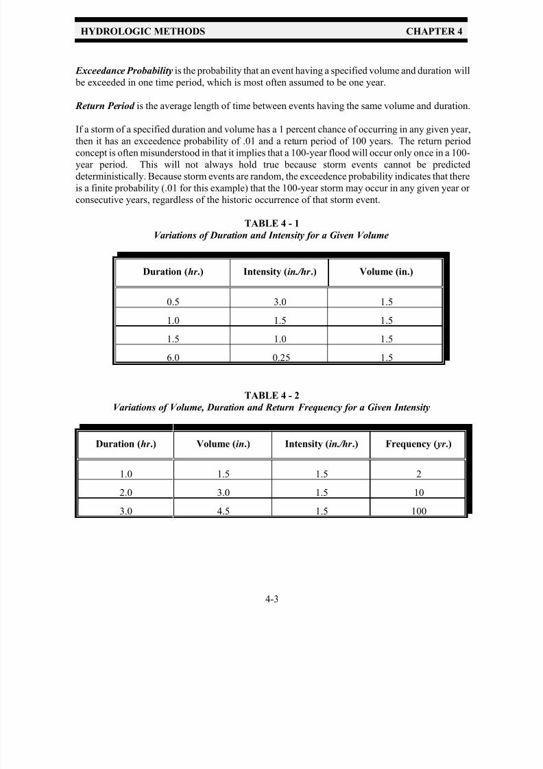
A specified amount of rainfall may occur from many different combinations of intensities and
durations, as shown in Table 4-1. Note that the peak intensity of runoff associated with each
combination will vary widely. Also, storm events with the same intensity may have significantly
different volumes and durations if the specified storm frequency (2-year, 10-year, 100-year) is
different, as shown in Table 4-2. It, therefore, becomes critical for any regulatory criteria to specify
the volume (or intensity) and the duration for a specified frequency design storm. Although
specifying one combination of volume and duration may limit the analysis, with regard to what is
considered to be the critical variable for any given watershed (erosion, flooding, water quality, etc.),
it does establish a baseline from which to work. (This analysis supports the SCS 24-hour design
storm since an entire range of storm intensities is incorporated into the rainfall distribution.)
Localities may choose to establish criteria based on specific watershed and receiving channel
conditions, which will dictate the appropriate design storm. (Refer to Channel Capacity/Channel
Design in Chapter 5, and MS-19 in the Virginia Erosion & Sediment Control Regulations.)
4-2.1 Frequency
The frequency of a specified design storm can be expressed either in terms of exceedence
probability or return period .
7/30/2019 Virginia Stormwater Managment Handbook Volume_II.pdf
http://slidepdf.com/reader/full/virginia-stormwater-managment-handbook-volumeiipdf 10/354
HYDROLOGIC METHODS CHAPTER 4
4-3
Exceedance Probability is the probability that an event having a specified volume and duration will
be exceeded in one time period, which is most often assumed to be one year.
Return Period is the average length of time between events having the same volume and duration.
If a storm of a specified duration and volume has a 1 percent chance of occurring in any given year,then it has an exceedence probability of .01 and a return period of 100 years. The return period
concept is often misunderstood in that it implies that a 100-year flood will occur only once in a 100-
year period. This will not always hold true because storm events cannot be predicted
deterministically. Because storm events are random, the exceedence probability indicates that there
is a finite probability (.01 for this example) that the 100-year storm may occur in any given year or
consecutive years, regardless of the historic occurrence of that storm event.
TABLE 4 - 1
Variations of Duration and Intensity for a Given Volume
Duration (hr .) Intensity (in./hr .) Volume (in.)
0.5 3.0 1.5
1.0 1.5 1.5
1.5 1.0 1.5
6.0 0.25 1.5
TABLE 4 - 2
Variations of Volume, Duration and Return Frequency for a Given Intensity
Duration (hr .) Volume (in.) Intensity (in./hr .) Frequency ( yr .)
1.0 1.5 1.5 2
2.0 3.0 1.5 10
3.0 4.5 1.5 100
7/30/2019 Virginia Stormwater Managment Handbook Volume_II.pdf
http://slidepdf.com/reader/full/virginia-stormwater-managment-handbook-volumeiipdf 11/354
HYDROLOGIC METHODS CHAPTER 4
4-4
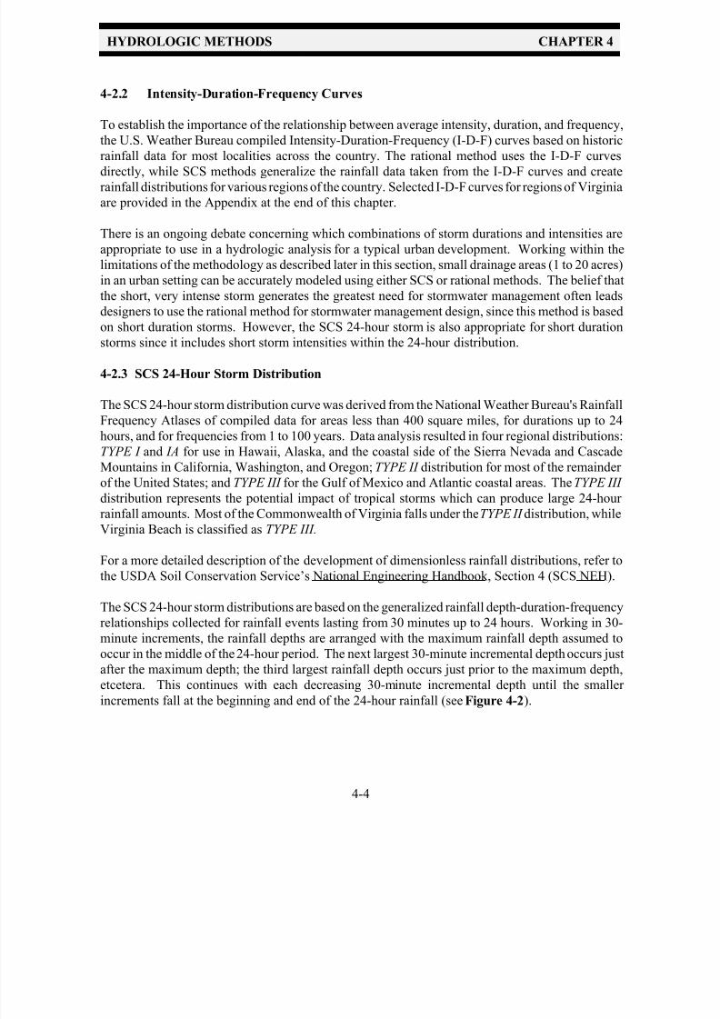
4-2.2 Intensity-Duration-Frequency Curves
To establish the importance of the relationship between average intensity, duration, and frequency,
the U.S. Weather Bureau compiled Intensity-Duration-Frequency (I-D-F) curves based on historic
rainfall data for most localities across the country. The rational method uses the I-D-F curves
directly, while SCS methods generalize the rainfall data taken from the I-D-F curves and createrainfall distributions for various regions of the country. Selected I-D-F curves for regions of Virginia
are provided in the Appendix at the end of this chapter.
There is an ongoing debate concerning which combinations of storm durations and intensities are
appropriate to use in a hydrologic analysis for a typical urban development. Working within the
limitations of the methodology as described later in this section, small drainage areas (1 to 20 acres)
in an urban setting can be accurately modeled using either SCS or rational methods. The belief that
the short, very intense storm generates the greatest need for stormwater management often leads
designers to use the rational method for stormwater management design, since this method is based
on short duration storms. However, the SCS 24-hour storm is also appropriate for short duration
storms since it includes short storm intensities within the 24-hour distribution.
4-2.3 SCS 24-Hour Storm Distribution
The SCS 24-hour storm distribution curve was derived from the National Weather Bureau's Rainfall
Frequency Atlases of compiled data for areas less than 400 square miles, for durations up to 24
hours, and for frequencies from 1 to 100 years. Data analysis resulted in four regional distributions:
TYPE I and IA for use in Hawaii, Alaska, and the coastal side of the Sierra Nevada and Cascade
Mountains in California, Washington, and Oregon; TYPE II distribution for most of the remainder
of the United States; and TYPE III for the Gulf of Mexico and Atlantic coastal areas. The TYPE III
distribution represents the potential impact of tropical storms which can produce large 24-hour
rainfall amounts. Most of the Commonwealth of Virginia falls under the TYPE II distribution, whileVirginia Beach is classified as TYPE III.
For a more detailed description of the development of dimensionless rainfall distributions, refer to
the USDA Soil Conservation Service’s National Engineering Handbook, Section 4 (SCS NEH).
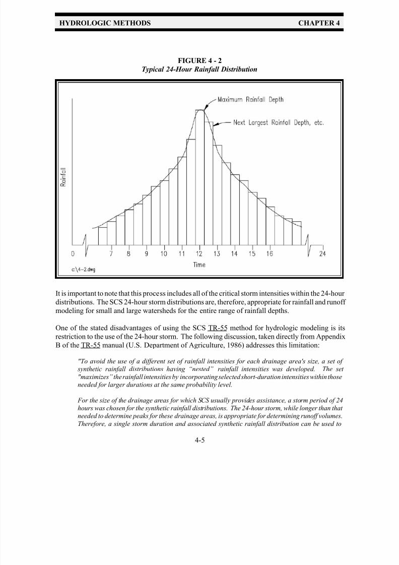
The SCS 24-hour storm distributions are based on the generalized rainfall depth-duration-frequency
relationships collected for rainfall events lasting from 30 minutes up to 24 hours. Working in 30-
minute increments, the rainfall depths are arranged with the maximum rainfall depth assumed to
occur in the middle of the 24-hour period. The next largest 30-minute incremental depth occurs just
after the maximum depth; the third largest rainfall depth occurs just prior to the maximum depth,
etcetera. This continues with each decreasing 30-minute incremental depth until the smaller
increments fall at the beginning and end of the 24-hour rainfall (see Figure 4-2).
7/30/2019 Virginia Stormwater Managment Handbook Volume_II.pdf
http://slidepdf.com/reader/full/virginia-stormwater-managment-handbook-volumeiipdf 12/354
HYDROLOGIC METHODS CHAPTER 4
4-5
FIGURE 4 - 2
Typical 24-Hour Rainfall Distribution
It is important to note that this process includes all of the critical storm intensities within the 24-hour
distributions. The SCS 24-hour storm distributions are, therefore, appropriate for rainfall and runoff
modeling for small and large watersheds for the entire range of rainfall depths.
One of the stated disadvantages of using the SCS TR-55 method for hydrologic modeling is its
restriction to the use of the 24-hour storm. The following discussion, taken directly from Appendix
B of the TR-55 manual (U.S. Department of Agriculture, 1986) addresses this limitation:
"To avoid the use of a different set of rainfall intensities for each drainage area's size, a set of
synthetic rainfall distributions having “nested” rainfall intensities was developed. The set
"maximizes” the rainfall intensities by incorporating selected short-duration intensities within thoseneeded for larger durations at the same probability level.
For the size of the drainage areas for which SCS usually provides assistance, a storm period of 24
hours was chosen for the synthetic rainfall distributions. The 24-hour storm, while longer than that
needed to determine peaks for these drainage areas, is appropriate for determining runoff volumes.
Therefore, a single storm duration and associated synthetic rainfall distribution can be used to
7/30/2019 Virginia Stormwater Managment Handbook Volume_II.pdf
http://slidepdf.com/reader/full/virginia-stormwater-managment-handbook-volumeiipdf 13/354
HYDROLOGIC METHODS CHAPTER 4
4-6
represent not only the peak discharges but also the runoff volumes for a range of drainage area
sizes.”
Figure 4-3 shows the SCS 24-hour rainfall distribution, which is a graph of the fraction of total
rainfall at any given time, t . Note that the peak intensity for the TYPE II distribution occurs
between time t = 11.5 hours and t = 12.5 hours.
FIGURE 4 - 3
SCS 24-Hour Rainfall Distribution
Source: USDA SCS
7/30/2019 Virginia Stormwater Managment Handbook Volume_II.pdf
http://slidepdf.com/reader/full/virginia-stormwater-managment-handbook-volumeiipdf 14/354
HYDROLOGIC METHODS CHAPTER 4
4-7
4-2.4 Synthetic Storms
The alternative to a given rainfall “distribution” is to input a custom design storm into the model.
This can be compiled from data gathered from a single rainfall event in a particular area, or a
synthetic storm created to test the response characteristics of a watershed under specific rainfall
conditions. Note, however, that a single historic design storm of known frequency is inadequate for the design of flood control structures, drainage systems, etc. The preferred procedure for such
design work is to synthesize data from the longest possible grouping of rainfall data and derive a
frequency relationship as described with the I-D-F curves.
4-2.5 Single Event vs. Continuous Simulation Computer Models
The fundamental requirement of a stormwater management plan is a quantitative analysis of the
watershed hydrology, hydraulics, and water quality, with consideration for associated facility costs.
Computers have greatly reduced the time required to complete such an analysis. Computers have
also greatly simplified the statistical analysis of compiled rainfall data.
In general, there are two main categories of hydrologic computer models: single-event computer
models and continuous-simulation models.
Single-event computer models require a minimum of one design-storm hyetograph as input. A
hyetograph is a graph of rainfall intensity on the vertical axis versus time on the horizontal axis, as
shown in Figure 4-4. A hyetograph shows the volume of precipitation at any given time as the area
beneath the curve, and the time-variation of the intensity.
The hyetograph can be a synthetic hyetograph or an historic storm hyetograph. When a frequency
or recurrence interval is specified for the input hyetograph, it is assumed that the resulting output
runoff has the same recurrence interval. (This is one of the general assumptions which is made for most single-event models.)
Continuous simulation models, on the other hand, incorporate the entire meteorologic record of a
watershed as their input, which may consist of decades of precipitation data. The data is processed
by the computer model, producing a continuous runoff hydrograph. The continuous hydrograph
output can be analyzed using basic statistical analysis techniques to provide discharge-frequency
relationships, volume-frequency relationships, flow-duration relationships, etc. The extent to which
the output hydrograph may be analyzed is dependent upon the input data available. The principal
advantage of the continuous simulation model is that it eliminates the need to choose a design storm,
instead providing long-term response data for a watershed which can then be statistically analyzed
for the desired frequency storm.
Computer advances have greatly reduced the analysis time and related expenses associated with
continuous models. It can be expected that future models, which combine some features of
continuous modeling with the ease of single-event modeling, will offer quick and more accurate
analysis procedures.

7/30/2019 Virginia Stormwater Managment Handbook Volume_II.pdf
http://slidepdf.com/reader/full/virginia-stormwater-managment-handbook-volumeiipdf 15/354
HYDROLOGIC METHODS CHAPTER 4
4-8
The hydrologic methods discussed in this handbook are limited to single-event methodologies,
based on historic data. Further information regarding the derivation of the I-D-F curves and the
SCS 24-hour rainfall distribution can be found in NEH, Section 4 - Hydrology.
FIGURE 4 - 4 Rainfall Hyetograph and Associated Runoff Hydrograph
4-3 RUNOFF HYDROGRAPHS
A runoff hydrograph is a graphical plot of the runoff or discharge from a watershed with respect
to time. Runoff occurring in a watershed flows downstream in various patterns which are influenced
by many factors, such as the amount and distribution of the rainfall, rate of snowmelt, stream
channel hydraulics, infiltration capacity of the watershed, and others, that are difficult to define. No
two flood hydrographs are alike.
Empirical relationships, however, have been developed from which complex hydrographs can be
derived. The critical element of the analysis, as with any hydrologic analysis, is the accurate

7/30/2019 Virginia Stormwater Managment Handbook Volume_II.pdf
http://slidepdf.com/reader/full/virginia-stormwater-managment-handbook-volumeiipdf 16/354
HYDROLOGIC METHODS CHAPTER 4
4-9
description of the watershed’s rainfall-runoff relationship, flow paths, and flow times. From this
data, runoff hydrographs can be generated.
This section provides a brief description of some of the types of hydrographs used for modeling
watersheds.
Natural hydrographs obtained directly from the flow records of a gauged stream.
Synthetic hydrographs obtained by using watershed parameters and storm characteristics to simulate
a natural hydrograph.
Unit hydrographs which are natural or synthetic hydrographs adjusted to represent one inch of
direct runoff.
Dimensionless unit hydrographs which are made to represent many unit hydrographs by using the
time to peak and the peak rates as basic units and plotting the hydrographs in ratios of these units.
4-3.1 Natural Hydrographs
Extensive watershed gauge data is required to develop a natural hydrograph. Frequently, the data
must be interpolated between points in order to provide a complete hydrograph. Stream gauge data
is very useful for calibrating models or synthetic hydrographs. However, the lack of such data often
eliminates the option of using a natural hydrograph.
4-3.2 Synthetic Hydrographs
A synthetic hydrograph is a hydrograph which is generated from the synthesis of data from a large
number of watersheds. The basis of a synthetic hydrograph is the establishment of a relationship
between the physical geometry of the watersheds and resulting hydrographs. The most commonly
used synthetic hydrograph for modeling and design is the unit hydrograph. The following section
briefly describes synthetic unit hydrograph methods.
4-3.3 Synthetic Unit Hydrographs
The unit hydrograph is the hydrograph that results from 1 inch of precipitation excess generated
uniformly over the watershed at a uniform rate during a specified time period.
The shape and characteristics of the runoff hydrograph for a given watershed are determined by the
specific characteristics of the storm and the physical characteristics of the watershed. Since the
physical characteristics of a watershed (shape, slope, ground cover, etc.) are constant, one might
expect considerable similarity in the shape of hydrographs from storms of similar rainfall

7/30/2019 Virginia Stormwater Managment Handbook Volume_II.pdf
http://slidepdf.com/reader/full/virginia-stormwater-managment-handbook-volumeiipdf 17/354
HYDROLOGIC METHODS CHAPTER 4
4-10
characteristics. This is the essence of the unit hydrograph. The unit hydrograph is a typical
hydrograph for a watershed where the runoff volume under the hydrograph is adjusted to equal 1
inch of equivalent depth over the watershed, as shown in Figure 4-5.
FIGURE 4 - 5 Typical Synthetic Unit Hydrograph
As mentioned, the unit hydrograph shape is also determined by the storm characteristics, such as
rainfall duration, time-intensity patterns, area distribution of rainfall, and depth of rainfall. The
following assumptions are made regarding the rainfall-runoff relationship when using a unit
hydrograph:
1. The runoff is from precipitation excess, the difference between precipitation and losses.
2. The volume of runoff is 1 inch , which is equal to the precipitation excess.
3. The precipitation excess is applied at a constant/uniform rate.
4. The excess is applied with uniform spatial distribution.

7/30/2019 Virginia Stormwater Managment Handbook Volume_II.pdf
http://slidepdf.com/reader/full/virginia-stormwater-managment-handbook-volumeiipdf 18/354
HYDROLOGIC METHODS CHAPTER 4
4-11
5. The intensity of rainfall excess is constant over the duration.
Many of these same assumptions are made when using almost any single-event hydrologic model.
These assumptions, however, do not hold true for all storms. Therefore, one can expect variations
in the ordinates of the unit hydrograph for different storms.
The unit hydrograph does not represent either the total runoff volume or the design hydrograph. The
unit hydrograph is simply used to translate the time distribution of precipitation excess into a runoff
hydrograph. In other words, the unit hydrograph provides the shape for the actual runoff
hydrograph. The physical characteristics of the watershed and the amount of precipitation excess,
as determined by the storm event and the rainfall-runoff relationship, will translate the unit
hydrograph into the actual runoff hydrograph. The peak discharge and the time to peak are
considered to be the defining parameters of the physical characteristics of the watershed. The unit
hydrograph is translated into an actual runoff hydrograph through a process called convolution,
which takes into account the peak and time to peak . The convolution process is an exercise in
multiplication, translation with time, and addition.
A unit hydrograph can be based on the analysis of a single watershed and can be used specifically
for that watershed. This is often the case when conducting flood studies for river basins. Rainfall-
runoff and streamflow data compiled within the watershed are analyzed and a unit hydrograph is
generated to better predict the response characteristics to various storm events. Generally, however,
basic streamflow and runoff data are not available to create a unit hydrograph for most development
projects. Therefore, techniques have been developed that allow for the generation of synthetic unit
hydrographs.
4-3.4 SCS Dimensionless Unit Hydrograph
The method developed by the Soil Conservation Service (SCS) for constructing synthetic unit
hydrographs is based on the dimensionless unit hydrograph. This dimensionless graph is the result
of an analysis of a large number of natural unit hydrographs from a wide range of watersheds
varying in size and geographic locations. This approach is based on using the watershed peak
discharge and time to peak discharge to relate the watershed characteristics to the dimensionless
hydrograph features. SCS methodologies provide various empirical equations, as discussed in this
chapter, to solve for the peak and time to peak for a given watershed. Various equations are then
used to define critical points on the hydrograph and thus define the runoff hydrograph. Figure 4-6
shows the SCS Dimensionless Unit Hydrograph. The critical points are the time to peak ,
represented by the watershed lag time, and the point of inflection, represented by the time of
concentration. The lag time of a watershed is the time from the center of mass of excess rainfall
to the time to peak of a unit hydrograph. The average relationship of lag, L, to time of concentration,
t c , is L = 0.6 t c . The reader is encouraged to read Chapters 15 and 16 of the National Engineering
Handbook, Section 4; Hydrology, for more information on unit hydrographs.
7/30/2019 Virginia Stormwater Managment Handbook Volume_II.pdf
http://slidepdf.com/reader/full/virginia-stormwater-managment-handbook-volumeiipdf 19/354
HYDROLOGIC METHODS CHAPTER 4
4-12
FIGURE 4 - 6
Dimensionless Curvilinear Unit Hydrograph and Equivalent Triangular Hydrograph
Source: NEH-4, Chapter 16
7/30/2019 Virginia Stormwater Managment Handbook Volume_II.pdf
http://slidepdf.com/reader/full/virginia-stormwater-managment-handbook-volumeiipdf 20/354
HYDROLOGIC METHODS CHAPTER 4
4-13
4-4 RUNOFF and PEAK DISCHARGE
The practice of estimating runoff as a fixed percentage of rainfall has been used in the design of
storm drainage systems for over 100 years. Despite its simplification of the complex rainfall - runoff
processes, it is still the most commonly used method for urban drainage calculations. It can be
accurate when drainage areas are subdivided into homogenious units, and when the designer hasenough data and experience to use the appropriate factors..
For watersheds or drainage areas comprised primarily of pervious cover such as open space, woods,
lawns, or agricultural land uses, the rainfall/runoff analysis becomes much more complex. Soil
conditions and types of vegetation are two of the variables that play a larger role in determining the
amount of rainfall which becomes runoff. In addition, other types of flow have a larger effect on
stream flow (and measured hydrograph) when the watershed is less urbanized. These are:
1. Surface runoff occurs only when the rainfall rate is greater than the infiltration rate and the
total volume of rainfall exceeds the interception, infiltration, and surface detention capacity
of the watershed. The runoff flows on the land surface collecting in the stream network.
2. Subsurface flow occurs when infiltrated rainfall meets an underground zone of low
transmission and travels above the zone to the soil surface to appear as a seep or spring.
3. Base flow occurs when there is a fairly steady flow into a stream channel from natural
storage. The flow comes from lakes or swamps, or from an aquifer replenished by infiltrated
rainfall or surface runoff.
In watershed hydrology, it is customary to deal separately with base flow and to combine all other
types of flow into direct runoff. Depending upon the requirements of the study, the designer can
calculate the peak flow rate, in cfs (cubic feet per second), of the direct runoff from the watershed,or determine the runoff hydrograph for the direct runoff from the watershed. A hydrograph is a
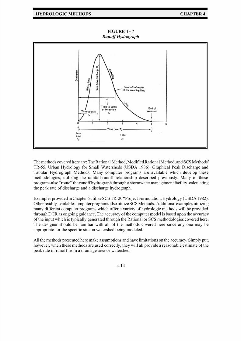
plot of discharge or runoff , on the vertical axis, versus time, on the horizontal axis, as shown in
Figure 4-7. A hydrograph shows the volume of runoff as the area beneath the curve, and the time-
variation of the discharge rate.
If the purpose of a hydrologic study is to measure the impact of various developments on the
drainage network within a watershed or to design flood control structures, then a hydrograph is
needed. If the purpose of a study is to design a roadway culvert or other simple drainage
improvement, then only the peak rate of flow is needed. Therefore, the purpose of a given study
will dictate the methodology which should be used. Procedures such as the Rational Method and
TR-55 Graphical Peak Discharge Method do not generate a runoff hydrograph. The TR-55
Tabular Method and the Modified Rational Method do generate runoff hydrographs.
This section will present some of the different methods for calculating runoff from a watershed.
Designers should be familiar with all of them since they require different types of input and generate
different types of results.
7/30/2019 Virginia Stormwater Managment Handbook Volume_II.pdf
http://slidepdf.com/reader/full/virginia-stormwater-managment-handbook-volumeiipdf 21/354
HYDROLOGIC METHODS CHAPTER 4
4-14
FIGURE 4 - 7
Runoff Hydrograph
The methods covered here are: The Rational Method, Modified Rational Method, and SCS Methods’
TR-55, Urban Hydrology for Small Watersheds (USDA 1986): Graphical Peak Discharge and
Tabular Hydrograph Methods. Many computer programs are available which develop these
methodologies, utilizing the rainfall-runoff relationship described previously. Many of these
programs also “route” the runoff hydrograph through a stormwater management facility, calculating
the peak rate of discharge and a discharge hydrograph.
Examples provided in Chapter 6 utilize SCS TR-20 “Project Formulation, Hydrology (USDA 1982).
Other readily available computer programs also utilize SCS Methods. Additional examples utilizing
many different computer programs which offer a variety of hydrologic methods will be provided
through DCR as ongoing guidance. The accuracy of the computer model is based upon the accuracy
of the input which is typically generated through the Rational or SCS methodologies covered here.
The designer should be familiar with all of the methods covered here since any one may be
appropriate for the specific site on watershed being modeled.
All the methods presented here make assumptions and have limitations on the accuracy. Simply put,
however, when these methods are used correctly, they will all provide a reasonable estimate of the
peak rate of runoff from a drainage area or watershed.
7/30/2019 Virginia Stormwater Managment Handbook Volume_II.pdf
http://slidepdf.com/reader/full/virginia-stormwater-managment-handbook-volumeiipdf 22/354
HYDROLOGIC METHODS CHAPTER 4
4-15
It should be noted that for small storm events (< 2" rainfall) TR-55 tends to underestimate the runoff,
while it has been shown to be fairly accurate for larger storm events (Pitt, 1994). Similarly, the
Rational formula has been found to be fairly accurate on smaller homogeneous watersheds, while
tending to lose accuracy in the larger more complex watersheds. The following discussion provides
further explanation of these methods, including assumptions, limitations, and information needed
for the analysis.
4-4.1 The Rational Method
The Rational Method was introduced in 1880 for determining peak discharges from drainage areas.
It is frequently criticized for its simplistic approach, but this same simplicity has made the Rational
Method one of the most widely used techniques today.
The Rational Formula estimates the peak rate of runoff at any location in a drainage area as a
function of the runoff coefficient , mean rainfall intensity, and drainage area. The Rational
Formula is expressed as follows:
Q = C I A
Equation 4-1
Rational Formula
where: Q = maximum rate of runoff, cfs
C = dimensionless runoff coefficient, dependent upon land use
I = design rainfall intensity, in inches per hour, for a duration equal to the timeof concentration of the watershed
A = drainage area, in acres
4-4.1.1 Assumptions
The Rational Method is based on the following assumptions:
1) Under steady rainfall intensity, the maximum discharge will occur at the watershed outlet
at the time when the entire area above the outlet is contributing runoff.
This “time” is commonly known as the time of concentration, t c , and is defined as the time required
for runoff to travel from the most hydrologically distant point in the watershed to the outlet.
The assumption of steady rainfall dictates that even during longer events, when factors such as

7/30/2019 Virginia Stormwater Managment Handbook Volume_II.pdf
http://slidepdf.com/reader/full/virginia-stormwater-managment-handbook-volumeiipdf 23/354
HYDROLOGIC METHODS CHAPTER 4
4-16
increasing soil saturation are ignored, the maximum discharge occurs when the entire watershed
is contributing to the peak flow, at time t = t c .
Furthermore, this assumption limits the size of the drainage area that can be analyzed using the
rational method. In large watersheds, the time of concentration may be so long that constant rainfall
intensities may not occur for long periods. Also, shorter, more intense bursts of rainfall that occur over portions of the watershed may produce large peak flows.
2) The time of concentration is equal to the minimum duration of peak rainfall .
The time of concentration reflects the minimum time required for the entire watershed to contribute
to the peak discharge as stated above. The rational method assumes that the discharge does not
increase as a result of soil saturation, decreased conveyance time, etc. (refer to Figure 4-8).
Therefore, the time of concentration is not necessarily intended to be a measure of the actual storm
duration, but simply the critical time period used to determine the average rainfall intensity from the
Intensity-Duration-Frequency curves.
3) The frequency or return period of the computed peak discharge is the same as the frequency
or return period of rainfall intensity (design storm) for the given time of concentration .
Frequencies of peak discharges depend not only on the frequency of rainfall intensity, but also the
response characteristics of the watershed. For small and mostly impervious areas, rainfall frequency
is the dominant factor since response characteristics are relatively constant. However, for larger
watersheds, the response characteristics will have a much greater impact on the frequency of the
peak discharge due to drainage structures, restrictions within the watershed, and initial rainfall losses
from interception and depression storage.
4) The fraction of rainfall that becomes runoff is independent of rainfall intensity or volume.
This assumption is reasonable for impervious areas, such as streets, rooftops, and parking lots. For
pervious areas, the fraction of rainfall that becomes runoff varies with rainfall intensity and the
accumulated volume of rainfall. As the soil becomes saturated, the fraction of rainfall that becomes
runoff will increase. This fraction is represented by the dimensionless runoff coefficient, C .
Therefore, the accuracy of the rational method is dependent on the careful selection of a coefficient
that is appropriate for the storm, soil, and land use conditions. Selection of appropriate C values will
be discussed later in this chapter.
It is easy to see why the rational method becomes more accurate as the percentage of impervious
cover in the drainage area approaches 100 percent.
5) The peak rate of runoff is sufficient information for the design of stormwater detention and
retention facilities.

7/30/2019 Virginia Stormwater Managment Handbook Volume_II.pdf
http://slidepdf.com/reader/full/virginia-stormwater-managment-handbook-volumeiipdf 24/354
HYDROLOGIC METHODS CHAPTER 4
4-17
4-4.1.2 Limitations
Because of the assumptions discussed above, the rational method should only be used when the
following criteria are met:
1) The given watershed has a time of concentration, t c , less than 20 minutes;
2) The drainage area is less than 20 acres.
For larger watersheds, attenuation of peak flows through the drainage network begins to be a factor
in determining peak discharge. While there are ways to adjust runoff coefficients (CN factors) to
account for the attenuation, or routing effects, it is better to use a hydrograph method or computer
simulation for these more complex situations.
Similarly, the presence of bridges, culverts, or storm sewers may act as restrictions which ultimately
impact the peak rate of discharge from the watershed. The peak discharge upstream of the
restriction can be calculated using a simple calculation procedure, such as the Rational Method,however a detailed storage routing procedure which considers the storage volume above the
restriction should be used to accurately determine the discharge downstream of the restriction.
4-4.1.3 Design Parameters
The following is a brief summary of the design parameters used in the rational method:
1) Time of concentration, tc
The most consistent source of error in the use of the rational method is the oversimplification of thetime of concentration calculation procedure. Since the origin of the rational method is rooted in the
design of culverts and conveyance systems, the main components of the time of concentration are
inlet time (or overland flow) and pipe or channel flow time. The inlet or overland flow time is
defined as the time required for runoff to flow overland from the furthest point in the drainage area
over the surface to the inlet or culvert. The pipe or channel flow time is defined as the time required
for the runoff to flow through the conveyance system to the design point. In addition, when an inlet
time of less than 5 minutes is encountered, the time is rounded up to 5 minutes, which is then used
to determine the rainfall intensity, I , for that inlet.
Variations in the time of concentration can impact the calculated peak discharge. When the
procedure for calculating the time of concentration is oversimplified, as mentioned above, theaccuracy of the Rational Method is greatly compromised. To prevent this oversimplification, it is
recommended that a more rigorous procedure for determining the time of concentration be used,
such as those outlined in Section 4-4.3.2 of this manual, Chapter 5 of the Virginia Erosion and
Sediment Control Handbook (VESCH), 1992 edition, Chapter 15, Section 4 of SCS National
Engineering Handbook, or the Virginia Department of Transportation (VDOT) drainage manual.

7/30/2019 Virginia Stormwater Managment Handbook Volume_II.pdf
http://slidepdf.com/reader/full/virginia-stormwater-managment-handbook-volumeiipdf 25/354
HYDROLOGIC METHODS CHAPTER 4
4-18
There are many procedures for estimating the time of concentration. Some were developed with a
specific type or size watershed in mind, while others were based on studies of a specific watershed.
The selection of any given procedure should include a comparison of the hydrologic and hydraulic
characteristics used in the formation of the procedure, versus the characteristics of the watershed
FIGURE 4 - 8
Rational Method Runoff Hydrograph
under study. The designer should be aware that if two or more methods of determining time of
concentration are applied to a given watershed, there will likely be a wide range in results. The SCS
method is recommended because it provides a means of estimating overland sheet flow time and
shallow concentrated flow time as a function of readily available parameters such as land slope and
land surface conditions. Regardless of which method is used, the result should be reasonable when
compared to an average flow time over the total length of the watershed.
2) Rainfall Intensity, I
The rainfall intensity, I , is the average rainfall rate, in inches per hour, for a storm duration equal to
the time of concentration for a selected return period (i.e., 1-year, 2-year, 10-year, 25-year, etc.).
Once a particular return period has been selected, and the time of concentration has been determined
for the drainage area, the rainfall intensity can be read from the appropriate rainfall Intensity-
7/30/2019 Virginia Stormwater Managment Handbook Volume_II.pdf
http://slidepdf.com/reader/full/virginia-stormwater-managment-handbook-volumeiipdf 26/354
HYDROLOGIC METHODS CHAPTER 4
4-19
Duration-Frequency (I-D-F) curve for the geographic area in which the drainage area is located.
These charts were developed from data furnished by the National Weather Service for regions of
Virginia, and are provided in the Appendix at the end of this chapter.
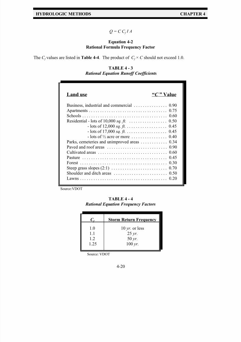
3) Runoff Coefficient, C
The runoff coefficients for different land uses within a watershed are used to generate a single,
weighted coefficient that will represent the relationship between rainfall and runoff for that
watershed. Recommended values can be found in Table 4-3. In an attempt to make the rational
method more accurate, efforts have been made to adjust the runoff coefficients to represent the
integrated effects of drainage basin parameters: land use, soil type, and average land slope. Table
4-3 provides recommended coefficients based on urban land use only, while Table 4-5 gives
recommended coefficients for various land uses based on soil type and land slope parameters.
A good understanding of these parameters is essential in choosing an appropriate coefficient. As
the slope of a drainage basin increases, runoff velocities increase for both sheet flow and shallow
concentrated flow. As the velocity of runoff increases, the ability of the surface soil to absorb therunoff decreases. This decrease in infiltration results in an increase in runoff. In this case, the
designer should select a higher runoff coefficient to reflect the increase due to slope.
Soil properties influence the relationship between runoff and rainfall even further since soils have
differing rates of infiltration. Historically, the Rational Method was used primarily for the design
of storm sewers and culverts in urbanizing areas; soil characteristics were not considered, especially
when the watershed was largely impervious. In such cases, a conservative design simply meant a
larger pipe and less headwater. For stormwater management purposes, however, the existing
condition (prior to development, usually with large amounts of pervious surfaces) often dictates the
allowable post-development release rate, and therefore, must be accurately modeled.
Soil properties can change throughout the construction process due to compaction, cut, and fill
operations. If these changes are not reflected in the runoff coefficient, the accuracy of the model
will decrease. Some localities arbitrarily require an adjustment in the runoff coefficient for pervious
surfaces due to the effects of construction on soil infiltration capacities. This is discussed in more
detail in Section 4-4.3 of this handbook. Such an adjustment is not possible using the Rational
Method since soil conditions are not considered. However, Table 4-5 attempts to provide a
graduated scale which correlates the rational method runoff coefficient with soil and land condition
characteristics.
4) Adjustment for Infrequent Storms
The Rational Method has undergone further adjustment to account for infrequent, higher intensity
storms. This adjustment is in the form of a frequency factor, C f , which accounts for the reduced
impact of infiltration and other effects on the amount of runoff during larger storms. With the
adjustment, the Rational Formula is expressed as follows:
7/30/2019 Virginia Stormwater Managment Handbook Volume_II.pdf
http://slidepdf.com/reader/full/virginia-stormwater-managment-handbook-volumeiipdf 27/354
HYDROLOGIC METHODS CHAPTER 4
4-20
Q = C C f I A
Equation 4-2
Rational Formula Frequency Factor
The C f values are listed in Table 4-4. The product of C f × C should not exceed 1.0.
TABLE 4 - 3
Rational Equation Runoff Coefficients
Land use “C ” Value
Business, industrial and commercial . . . . . . . . . . . . . . . 0.90
Apartments . . . . . . . . . . . . . . . . . . . . . . . . . . . . . . . . . . . 0.75
Schools . . . . . . . . . . . . . . . . . . . . . . . . . . . . . . . . . . . . . . 0.60
Residential - lots of 10,000 sq. ft. . . . . . . . . . . . . . . . . . 0.50
- lots of 12,000 sq. ft. . . . . . . . . . . . . . . . . . . 0.45
- lots of 17,000 sq. ft. . . . . . . . . . . . . . . . . . . 0.45
- lots of ½ acre or more . . . . . . . . . . . . . . . . 0.40
Parks, cemeteries and unimproved areas . . . . . . . . . . . . 0.34
Paved and roof areas . . . . . . . . . . . . . . . . . . . . . . . . . . . 0.90
Cultivated areas . . . . . . . . . . . . . . . . . . . . . . . . . . . . . . . 0.60
Pasture . . . . . . . . . . . . . . . . . . . . . . . . . . . . . . . . . . . . . . 0.45
Forest . . . . . . . . . . . . . . . . . . . . . . . . . . . . . . . . . . . . . . . 0.30
Steep grass slopes (2:1) . . . . . . . . . . . . . . . . . . . . . . . . . 0.70
Shoulder and ditch areas . . . . . . . . . . . . . . . . . . . . . . . . 0.50
Lawns . . . . . . . . . . . . . . . . . . . . . . . . . . . . . . . . . . . . . . . 0.20
Source:VDOT
TABLE 4 - 4
Rational Equation Frequency Factors
C f Storm Return Frequency
1.01.1
1.2
1.25
10 yr. or less25 yr.
50 yr.
100 yr.
Source: VDOT
7/30/2019 Virginia Stormwater Managment Handbook Volume_II.pdf
http://slidepdf.com/reader/full/virginia-stormwater-managment-handbook-volumeiipdf 28/354
HYDROLOGIC METHODS CHAPTER 4
4-21
T A B L E
4 - 5 a
R a t i o n a l E q u a t i o n C o e f f i c i e n t s f o r S C S H y d r o l o g i c S o
i l G r o u p s ( A , B , C , D )
U r b a n L a n d U s e s
S T O R M F R E Q U E N C I E S O F L E S S T H A N 2 5 Y E A R S
L a n d U s e
H y d r o l o g i c
C o n d i t i o n
H Y D R O L O G I C S O I L
G R O U P / S L O P E
A
B
C
D
0 - 2 %
2 - 6 %
6 % +
0 - 2 %
2 - 6 %
6 % + 0
- 2 %
2 - 6 %
6 % +
0 - 2 %
2 - 6 %
6 % +
P a v e d A r e a s a n d
I m p e r v i o u s
S u r f a c e s
0 . 9 0
0 . 9 0
0 . 9 0
0 . 9 0
0 . 9 0
0 . 9 0
0 . 9 0
0 . 9 0
0 . 9 0
0 . 9 0
0 . 9 0
0 . 9 0
O p e n S p a c e ,
L a w n s , e t c .
G o o d
0 . 0 8
0 . 1 2
0 . 1 5
0 . 1 1
0 . 1 6
0 . 2 1
0 . 1 4
0 . 1 9
0 . 2 4
0 . 2 0
0 . 2 4
0 . 2 8
I n d u s t r i a l
0 . 6 7
0 . 6 8
0 . 6 8
0 . 6 8
0 . 6 8
0 . 6 9
0 . 6 8
0 . 6 9
0 . 6 9
0 . 6 9
0 . 6 9
0 . 7 0
C o m m e r c i a l
0 . 7 1
0 . 7 1
0 . 7 2
0 . 7 1
0 . 7 2
0 . 7 2
0 . 7 2
0 . 7 2
0 . 7 2
0 . 7 2
0 . 7 2
0 . 7 2
R e s i d e n t i a l
L o t S i z e 1 / 8
A c r e
0 . 2 5
0 . 2 8
0 . 3 1
0 . 2 7
0 . 3 0
0 . 3 5
0 . 3 0
0 . 3 3
0 . 3 8
0 . 3 3
0 . 3 6
0 . 4 2
L o t S i z e 1 / 4
A c r e
0 . 2 2
0 . 2 6
0 . 2 9
0 . 2 4
0 . 2 9
0 . 3 3
0 . 2 7
0 . 3 1
0 . 3 6
0 . 3 0
0 . 3 4
0 . 4 0
L o t S i z e 1 / 3
A c r e
0 . 1 9
0 . 2 3
0 . 2 6
0 . 2 2
0 . 2 6
0 . 3 0
0 . 2 5
0 . 2 9
0 . 3 4
0 . 2 8
0 . 3 2
0 . 3 9
L o t S i z e ½
A c r e
0 . 1 6
0 . 2 0
0 . 2 4
0 . 1 9
0 . 2 3
0 . 2 8
0 . 2 2
0 . 2 7
0 . 3 2
0 . 2 6
0 . 3 0
0 . 3 7
L o t S i z e 1 . 0
A c r e
0 . 1 4
0 . 1 9
0 . 2 2
0 . 1 7
0 . 2 1
0 . 2 6
0 . 2 0
0 . 2 5
0 . 3 1
0 . 2 4
0 . 2 9
0 . 3 5
S o u r c e : M a r y l a n d S t a t e H i g h w a y A d m i n i s t r
a t i o n
7/30/2019 Virginia Stormwater Managment Handbook Volume_II.pdf
http://slidepdf.com/reader/full/virginia-stormwater-managment-handbook-volumeiipdf 29/354
HYDROLOGIC METHODS CHAPTER 4
4-22
T A B L E
4 - 5 b
R a t i o n a l E q u a t i o n C o e f f
i c i e n t s f o r S C S H y d r o l o g i c S o i l G r o u p s ( A , B , C , D )
R u r a l L a n d U s e s
S T O R M F R E Q U E N C I E S O F L E S S T H A N 2 5 Y E A R S
L a n d U s e
T r e a t m e n t
/
P r a c t i c e
H y d r o l o g i
c
C o n d i t i o n
H Y D R O L O G I C S O
I L G R O U P / S L O P E
A
B
C
D
0 - 2 %
2 - 6 %
6 % +
0 - 2 %
2 - 6 %
6 % +
0 - 2 %
2 - 6 %
6 % +
0 - 2 %
2 - 6 %
6 % +
P a s t u r e o r
R a n g e
G o o d
0 . 0 7
0 . 0 9
0 . 1 0
0 . 1 8
0 . 2 0
0 . 2 2
0 . 2 7
0 . 2 9
0 . 3 1
0 . 3 2
0 . 3 4
0 . 3 5
C o n t o u r e d
G o o d
0 . 0 3
0 . 0 4
0 . 0 6
0 . 1 1
0 . 1 2
0 . 1 4
0 . 2 4
0 . 2 6
0 . 2 8
0 . 3 1
0 . 3 3
0 . 3 4
M e a d o w
0 . 0 6
0 . 0 8
0 . 1 0
0 . 1 0
0 . 1 4
0 . 1 9
0 . 1 2
0 . 1 7
0 . 2 2
0 . 1 5
0 . 2 0
0 . 2 5
W o o d e d
G o o d
0 . 0 5
0 . 0 7
0 . 0 8
0 . 0 8
0 . 1 1
0 . 1 5
0 . 1 0
0 . 1 3
0 . 1 7
0 . 1 2
0 . 1 5
0 . 2 1
S o u r c e : M a r y l a n d S t a t e H i g h w a y A d m i n i s t r a t i o n

7/30/2019 Virginia Stormwater Managment Handbook Volume_II.pdf
http://slidepdf.com/reader/full/virginia-stormwater-managment-handbook-volumeiipdf 30/354
HYDROLOGIC METHODS CHAPTER 4
4-23
T A B L E
4 - 5 c
R a t i o n a l E q u a t i o n C o e f f i c i e n t s f o r S C S H y d r o l o g i c S o
i l G r o u p s ( A , B , C , D )
A g r i c u l t u r a l L a n d U s e s
S T O R M F
R E Q U E N C I E S O F L E S S T H A N 2 5
Y E A R S
L a n d
U s e
T r e a t m e n t /
P r a c t i c e
H y d r o l o g i c
C o n d i t i o n
H Y D R O L O G I C S O I L G R O U P / S L O P E
A
B
C
D
0 - 2 %
2 - 6 %
6 % +
0 - 2 %
2 - 6 %
6 % +
0 - 2 %
2 - 6 %
6 % +
0 - 2 %
2 - 6 %
6 % +
F a l l o w
S t r a i g h t R o w
0 . 4 1
0 . 4 8
0 . 5 3
0 . 6 0
0 . 6 6
0 . 7 1
0 . 7 2
0 . 7 8
0 . 8 2
0 . 8 4
0 . 8 8
0 . 9 1
R o w
C r o p s
S t r a i g h t R o w
G o o d
0 . 2 4
0 . 3 0
0 . 3 5
0 . 4 3
0 . 4 8
0 . 5 2
0 . 6 1
0 . 6 5
0 . 6 8
0 . 7 3
0 . 7 6
0 . 7 8
C o n t o u r e d
G o o d
0 . 2 1
0 . 2 6
0 . 3 0
0 . 4 1
0 . 4 5
0 . 4 9
0 . 5 5
0 . 5 9
0 . 6 3
0 . 6 3
0 . 6 6
0 . 6 8
C o n t o u r e d
a n d T e r r a c e d
G o o d
0 . 2 0
0 . 2 4
0 . 2 7
0 . 3 1
0 . 3 5
0 . 3 9
0 . 4 5
0 . 4 8
0 . 5 1
0 . 5 5
0 . 5 8
0 . 6 0
S m a l l
G r a i n
S t r a i g h t R o w
G o o d
0 . 2 3
0 . 2 6
0 . 2 9
0 . 4 2
0 . 4 5
0 . 4 8
0 . 5 7
0 . 6 0
0 . 6 2
0 . 7 1
0 . 7 3
0 . 7 5
S o u r c e : M a r y l a n d S t a t e H i g h w a y A d m i n i s t r a t i o n
7/30/2019 Virginia Stormwater Managment Handbook Volume_II.pdf
http://slidepdf.com/reader/full/virginia-stormwater-managment-handbook-volumeiipdf 31/354
HYDROLOGIC METHODS CHAPTER 4
4-24
T A B L E
4 - 5 d
R a t i o n a l E q u a t i o n C o e f f i c i e n t s f o r S C S H y d r o l o g i c S o i l G r o u p s ( A , B , C , D )
A g r i c u l t u r a l L a n d U s e s
S T O R M
F R E Q U E N C I E S O F L E S S T H A N
2 5 Y E A R S
L a n d U s e
T r e a t m e n t /
P r a c t i c e
H y d r o l o g i
c
C o n d i t i o n
H Y D R O L O G I C S O I L G R O U P / S L O P E
A
B
C
D
0 - 2
%
2 - 6 %
6 % +
0 - 2 %
2 - 6 %
6
% +
0 - 2 %
2 - 6 %
6 % +
0 - 2 %
2 - 6 %
6 % +
S m a l l
G r a i n
C o n t o u r e d
G o o d
0 . 1
7
0 . 2 2
0 . 2 7
0 . 3 3
0 . 3 8
0 . 4 2
0 . 5 4
0 . 5 8
0 . 6 1
0 . 6 2
0 . 6 5
0 . 6 7
C o n t o u r e d
a n d T e r r a c e d
G o o d
0 . 1
6
0 . 2 0
0 . 2 4
0 . 3 1
0 . 3 5
0 . 3 8
0 . 4 5
0 . 4 8
0 . 5 0
0 . 5 5
0 . 5 8
0 . 6 0
C l o s e d -
s e e d e d
L e g u m e s
o r R o t a t i o n
M e a d o w
S t r a i g h t
R o w
G o o d
0 . 1
5
0 . 1 9
0 . 2 3
0 . 3 1
0 . 3 5
0 . 3 8
0 . 5 5
0 . 5 8
0 . 6 0
0 . 6 3
0 . 6 5
0 . 6 6
C o n t o u r e d
G o o d
0 . 1
4
0 . 1 8
0 . 2 1
0 . 3 0
0 . 3 4
0 . 3 7
0 . 4 5
0 . 4 8
0 . 5 1
0 . 5 8
0 . 6 0
0 . 6 1
C o n t o u r e d
a n d T e r r a c e d
G o o d
0 . 0
7
0 . 1 0
0 . 1 3
0 . 2 8
0 . 3 2
0 . 3 5
0 . 4 4
0 . 4 7
0 . 4 9
0 . 5 2
0 . 5 4
0 . 5 6
S o u
r c e : M a r y l a n d S t a t e H i g h w a y A d m i n i s t r a t i o n

7/30/2019 Virginia Stormwater Managment Handbook Volume_II.pdf
http://slidepdf.com/reader/full/virginia-stormwater-managment-handbook-volumeiipdf 32/354
HYDROLOGIC METHODS CHAPTER 4
4-25
4-4.2 Modified Rational Method
The modified rational method is a variation of the rational method, developed mainly for the sizing
of detention facilities in urban areas. The modified rational method is applied similarly to the
rational method except that it utilizes a fixed rainfall duration. The selected rainfall duration
depends on the requirements of the user. For example, the designer might perform an iterativecalculation to determine the rainfall duration which produces the maximum storage volume
requirement when sizing a detention basin. This procedure will be discussed later in Chapter 5,
Hydraulic Calculations.
4-4.2.1 Assumptions
The modified rational method is based on the following assumptions:
1. All of the assumptions used with the rational method apply. The most significant difference
is that the time of concentration for the modified rational method is equal to the rainfall
intensity averaging period rather than the actual storm duration.
This assumption means that any rainfall, or any runoff generated by the rainfall, that occurs before
or after the rainfall averaging period is unaccounted for. Thus, when used as a basin sizing
procedure, the modified rational method may seriously underestimate the required storage
volume. (Walesh, 1989)
2) The runoff hydrograph for a watershed can be approximated as triangular or trapezoidal
in shape.
This assumption implies a linear relationship between peak discharge and time for any and all
watersheds.
4-4.2.2 Limitations
All of the limitations listed for the rational method apply to the modified rational method. The key
difference is the assumed shape of the resulting runoff hydrograph. The rational method produces
a triangular shaped hydrograph, while the modified rational method can generate triangular or
trapezoidal hydrographs for a given watershed, as shown in Figure 4-9.
4-4.2.3 Design Parameters
The equation Q = C I A (the rational equation) is used to calculate the peak discharge for all three
hydrographs shown in Figure 4-9. Notice that the only difference between the rational method and
the modified rational method is the incorporation of the storm duration, d , into the modified rational
method to generate a volume of runoff in addition to the peak discharge.

7/30/2019 Virginia Stormwater Managment Handbook Volume_II.pdf
http://slidepdf.com/reader/full/virginia-stormwater-managment-handbook-volumeiipdf 33/354
HYDROLOGIC METHODS CHAPTER 4
4-26
Type 1 - Storm duration, d , is equal to the time of concentration, t c.
Type 2 - Storm duration, d , is greater than the time of concentration, t c.
Type 3 - Storm duration, d , is less than the time of concentration, t c.
FIGURE 4 - 9
Modified Rational Method Runoff Hydrographs
Source: Urban Surface Water Management, Walesh, Stuart G.
The rational method generates the peak discharge that occurs when the entire watershed is
contributing to the peak (at a time t = t c) and ignores the effects of a storm which lasts longer than
time t . The modified rational method, however, considers storms with a longer duration than the
watershed t c , which may have a smaller or larger peak rate of discharge, but will produce a greater
volume of runoff (area under the hydrograph) associated with the longer duration of rainfall. Figure
4-10 shows a family of hydrographs representing storms of different durations. The storm duration
which generates the greatest volume of runoff may not necessarily produce the greatest peak rate
of discharge.
Note that the duration of the receding limb of the hydrograph is set to equal the time of
concentration, t c , or 1.5 times t c . The direct solution, which will be discussed in Chapter 5, uses
1.5t c as the receding limb. This is justified since it is more representative of actual storm and runoff
dynamics. (It is also more similar to the SCS unit hydrograph where the receding limb extends
longer than the rising limb.) Using 1.5 times t c in the direct solution methodology provides for
a more conservative design and will be used in this manual.
7/30/2019 Virginia Stormwater Managment Handbook Volume_II.pdf
http://slidepdf.com/reader/full/virginia-stormwater-managment-handbook-volumeiipdf 34/354
HYDROLOGIC METHODS CHAPTER 4
4-27
The modified rational method allows the designer to analyze several different storm durations to
determine the one that requires the greatest storage volume with respect to the allowable release rate.
This storm duration is referred to as the critical storm duration and is used as a basin sizing tool.
The technique is discussed in more detail in Chapter 5 of this handbook.
FIGURE 4 - 10 Modified Rational Method Family of Runoff Hydrographs
4-4.3 SCS Methods - TR-55 Estimating Runoff
The U.S. Soil Conservation Service published Technical Release Number 55 (TR-55), 2nd edition,
in June of 1986, entitled Urban Hydrology for Small Watersheds. The techniques outlined in TR-55
require the same basic data as the rational method: drainage area, time of concentration, land use and
rainfall. The SCS approach, however, is more sophisticated in that it allows the designer to
manipulate the time distribution of the rainfall, the initial rainfall losses to interception and
depression storage, and the moisture condition of the soils prior to the storm.
The procedures developed by SCS are based on a dimensionless rainfall distribution curve for a 24-
hour storm, as described in Section 4-2.3.
7/30/2019 Virginia Stormwater Managment Handbook Volume_II.pdf
http://slidepdf.com/reader/full/virginia-stormwater-managment-handbook-volumeiipdf 35/354
HYDROLOGIC METHODS CHAPTER 4
4-28
TR-55 presents two general methods for estimating peak discharges from urban watersheds: the
graphical method and the tabular method . The graphical method is limited to watersheds whose
runoff characteristics are fairly uniform and whose soils, land use, and ground cover can be
represented by a single Runoff Curve Number (CN ). The graphical method provides a peak
discharge only and is not applicable for situations where a hydrograph is required.
The tabular method is a more complete approach and can be used to develop a hydrograph at any
point in a watershed. For large areas it may be necessary to divide the area into sub-watersheds to
account for major land use changes, analyze specific study points within sub-watersheds, or locate
stormwater drainage facilities and assess their effects on peak flows. The tabular method can
generate a hydrograph for each sub-watershed for the same storm event. The hydrographs can then
be routed through the watershed and combined to produce a partial composite hydrograph at the
selected study point. The tabular method is particularly useful in evaluating the effects of an altered
land use in a specific area within a given watershed.
Prior to using either the graphical or tabular methods, the designer must determine the volume of
runoff resulting from a given depth of precipitation and the time of concentration, t c , for thewatershed being analyzed. The methods for determining these values will be discussed briefly in
this section. However, the reader is strongly encouraged to obtain a copy of the TR-55 manual from
the Soil Conservation Service to gain more insight into the procedures and limitations.
The SCS Runoff Curve Number (CN) Method is used to estimate runoff. This method is described
in detail in the SCS National Engineering Handbook, Section 4 (SCS 1985). The runoff equation
(found in TR-55 and discussed later in this section) provides a relationship between runoff and
rainfall as a function of the CN . The CN is a measure of the land's ability to infiltrate or otherwise
detain rainfall, with the excess becoming runoff. The CN is a function of the land cover (woods,
pasture, agricultural use, percent impervious, etc.), hydrologic condition, and soils.
4-4.3.1 Limitations
1. TR-55 has simplified the relationship between rainfall and runoff by reducing all of the initial
losses before runoff begins, or initial abstraction, to the term I a , and approximating the soil
and cover conditions using the variable S, potential maximum retention. Both of these terms,
I a and S, are functions of the runoff curve number.
Runoff curve numbers describe average conditions that are useful for design purposes. If the
purpose of the hydrologic study is to model a historical storm event, average conditions may not be
appropriate.
2. The designer should understand the assumption reflected in the initial abstraction term, I a.
I a represents interception, initial infiltration, surface depression storage, evapotranspiration,
and other watershed factors and is generalized as a function of the runoff curve number based
on data from agricultural watersheds.

7/30/2019 Virginia Stormwater Managment Handbook Volume_II.pdf
http://slidepdf.com/reader/full/virginia-stormwater-managment-handbook-volumeiipdf 36/354
HYDROLOGIC METHODS CHAPTER 4
4-29
This can be especially important in an urban application because the combination of impervious area
with pervious area can imply a significant initial loss that may not take place. On the other hand,
the combination of impervious and pervious area can underestimate initial losses if the urban area
has significant surface depression storage. (To use a relationship other than the one established in
TR-55, the designer must redevelop the runoff equation by using the original rainfall-runoff data to
establish new curve number relationships for each cover and hydrologic soil group. This wouldrepresent a large data collection and analysis effort.)
3. Runoff from snowmelt or frozen ground cannot be estimated using these procedures.
4. The runoff curve number method is less accurate when the runoff is less than 0.5 inch. As a
check, use another procedure to determine runoff.
5. The SCS runoff procedures apply only to surface runoff and do not consider subsurface flow
or high groundwater.
6. Manning’s kinematic solution ( Chapter 4-4.3.3.E ) should not be used to calculate the time of concentration for sheet flow longer than 300 feet. This limitation will affect the time of
concentration calculations. Note that many jurisdictions consider 150 feet to be the maximum
length of sheet flow before shallow concentrated flow develops.
7. The minimum t c used in TR-55 is 0.1 hour.
4-4.3.2 Information Needed
Generally a good understanding of the physical characteristics of the watershed is needed to solve
the runoff equation and determine the time of concentration. Some features, such as topography andchannel geometry can be obtained from topographic maps such as the USGS 1" = 2000' quadrangle
maps. Various sources of information may be accurate enough for a watershed study, however, the
accuracy of the study will be directly related to the accuracy and level of detail of the base
information. Ideally, a site investigation and field survey should be conducted to verify specific
features such as channel geometry and material, culvert sizes, drainage divides, ground cover, etc.
Depending on the size and scope of the study, however, a site investigation may not be economically
feasible.
The data needed to solve the runoff equation and determine the watershed time of concentration,
t c , and travel time, T t , is listed below. These items are discussed in more detail in Section 4-4.3.3.
1. Soil information (to determine the hydrologic soil group).
2. Ground cover type (impervious, woods, grass, etc.).
3. Treatment (cultivated or agricultural land).
7/30/2019 Virginia Stormwater Managment Handbook Volume_II.pdf
http://slidepdf.com/reader/full/virginia-stormwater-managment-handbook-volumeiipdf 37/354
HYDROLOGIC METHODS CHAPTER 4
4-30
4. Hydrologic condition (for design purposes, the hydrologic condition should be considered
"GOOD" for the pre-developed condition).
5. Urban impervious area modifications (connected, unconnected, etc.).
6. Topography – detailed enough to accurately identify drainage divides, t c and T t flow pathsand channel geometry, and surface condition (roughness coefficient).
4-4.3.3 Design Parameters
A. Soils
In hydrograph applications, runoff is often referred to as rainfall excess or effective rainfall ,
and is defined as the amount of rainfall that exceeds the land’s capability to infiltrate or
otherwise retain the rainwater. The soil type or classification, the land use and land treatment,
and the hydrologic condition of the cover are the watershed factors that will have the mostsignificant impact on estimating the volume of rainfall excess, or runoff.
HYDROLOGIC SOIL GROUP CLASSIFICATION
SCS has developed a soil classification system that consists of four groups, identified as A,
B, C , and D. Soils are classified into one of these categories based upon their minimum
infiltration rate. By using information obtained from local SCS offices, soil and water
conservation district offices, or from SCS Soil Surveys (published for many counties across
the country), the soils in a given area can be identified. Preliminary soil identification is
especially useful for watershed analysis and planning in general. When preparing a stormwater
management plan for a specific site, it is recommended that soil borings be taken to verify thehydrologic soil classification. Virginia soils and their respective Hydrologic Soil Group
( HSG ) classifications are provided in the Appendix at the end of this Chapter, as well as
VESCH, 1992 edition. TR-55 contains similar information for soils across the United States.
Soil characteristics associated with each Hydrologic Soil Group are generally described as
follows:
Group A: Soils with low runoff potential due to high infiltration rates, even when thoroughly
wetted. These soils consist primarily of deep, well to excessively drained sands and gravels
with high water transmission rates (0.30 in./hr.). Group A soils include sand, loamy sand,
or sandy loam.
Group B: Soils with moderately low runoff potential due to moderate infiltration rates when
thoroughly wetted. These soils consist primarily of moderately deep to deep, and moderately
well to well-drained soils. Group B soils have moderate water transmission rates (0.15-0.30
in./hr.) and include silt loam or loam.

7/30/2019 Virginia Stormwater Managment Handbook Volume_II.pdf
http://slidepdf.com/reader/full/virginia-stormwater-managment-handbook-volumeiipdf 38/354
HYDROLOGIC METHODS CHAPTER 4
4-31
Group C: Soils with moderately high runoff potential due to slow infiltration rates when
thoroughly wetted. These soils typically have a layer near the surface that impedes the
downward movement of water or soils. Group C soils have low water transmission rates
(0.05-0.15 in./hr.) and include sandy clay loam.
Group D: Soils with high runoff potential due to very slow infiltration rates. These soilsconsist primarily of clays with high swelling potential, soils with permanently high water
tables, soils with a claypan or clay layer at or near the surface, and shallow soils over nearly
impervious parent material. Group D soils have very low water transmission rates (0-0.05
in./hr.) and include clay loam, silty clay loam, sandy clay, silty clay, or clay.
Any disturbance of a soil profile can significantly alter the soil’s infiltration characteristics.
With urbanization, the hydrologic soil group for a given area can change due to soil mixing,
introduction of fill material from other areas, removal of material during mass grading
operations, or compaction from construction equipment. A layer of topsoil may typically be
saved and replaced after the earthwork is completed, but the native underlying soils have been
dramatically altered. Therefore, any disturbed soil should be classified by its physicalcharacteristics as given above for each soil group.
Some jurisdictions require all site developments to be analyzed using an HSG classification
that is one category below the actual pre-developed HSG . For example, a site with a pre-
developed HSG classification of B, as determined from the soil survey, would be analyzed in
its developed state using an HSG classification of C .
B. Hydrologic Condition
Hydrologic condition represents the effects of cover type and treatment on infiltration and
runoff. It is generally estimated from the density of plant and residue cover across the
drainage area. Good hydrologic condition indicates that the cover has a low runoff potential,
while poor hydrologic condition indicates that the cover has a high runoff potential.
Hydrologic condition is used in describing non-urbanized lands such as woods, meadow,
brush, agricultural land, and open spaces associated with urbanized areas, such as lawns,
parks, golf courses, and cemeteries. Treatment is a cover type modifier to describe the
management of cultivated agricultural lands. Table 4-6(a,b) provides an excerpt from Table
2-2 in TR-55 which shows the treatment and hydrologic condition for various land uses.
When a watershed is being analyzed to determine the impact of proposed development,
Virginia’s stormwater management regulations require the designer to consider all
existing or undeveloped land to be in hydrologically good condition. This results in lower
existing condition peak runoff rates which, in turn, results in greater post-development peak
control. In most cases, undeveloped land is in good hydrologic condition unless it has been
altered in some way. Since the goal of most stormwater programs is to reduce the peak flows

7/30/2019 Virginia Stormwater Managment Handbook Volume_II.pdf
http://slidepdf.com/reader/full/virginia-stormwater-managment-handbook-volumeiipdf 39/354
HYDROLOGIC METHODS CHAPTER 4
4-32
A decision to use “wet” or “dry” antecedent runoff conditions should be
based on thorough field work, such as carefully monitored rain gauge data.
from developed or altered areas to their pre-developed or pre-altered rates, this is a reasonable
approach. In addition this approach eliminates any inconsistencies in judging the condition
of undeveloped land or open space.
C. Runoff Curve Number (CN) Determination
The soil group classification, cover type and the hydrologic condition are used to determine
the runoff curve number, CN . The CN indicates the runoff potential of an area when the
ground is not frozen. Table 4-6(a,b), excerpted from TR-55,provides the RCNs for various
land use types and soil groups. (A more complete table can be found in TR-55.)
Several factors should be considered when choosing an CN for a given land use. First, the designer
should realize that the curve numbers in Table 4-6 and TR-55 are for the average antecedent runoff
or moisture condition, ARC . The ARC is the index of runoff potential before a storm event and can
have a major impact on the relationship between rainfall and runoff for a watershed. Average ARC
implies that the soils are neither very wet nor very dry when the design storm begins. Average ARC
runoff curve numbers can be converted to dry or wet values, however the average antecedent runoff condition is recommended for design purposes.
It is also important to consider the list of assumptions made in developing the runoff curve numbers
as provided in Table 4-6 and in TR-55. Some of these assumptions are outlined below.
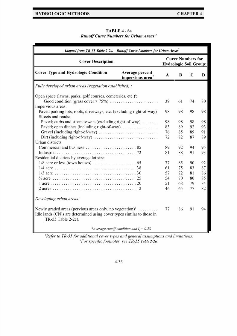
7/30/2019 Virginia Stormwater Managment Handbook Volume_II.pdf
http://slidepdf.com/reader/full/virginia-stormwater-managment-handbook-volumeiipdf 40/354
HYDROLOGIC METHODS CHAPTER 4
4-33
TABLE 4 - 6a
Runoff Curve Numbers for Urban Areas 1
Adapted from TR-55 Table 2-2a. --Runoff Curve Numbers for Urban Areas*
Cover DescriptionCurve Numbers for
Hydrologic Soil Group:
Cover Type and Hydrologic Condition Average percent
impervious area2 A B C D
Fully developed urban areas (vegetation established) :
Open space (lawns, parks, golf courses, cemeteries, etc.)2:
Good condition (grass cover > 75%) . . . . . . . . . . . . . . . . . . . . . .
Impervious areas:
Paved parking lots, roofs, driveways, etc. (excluding right-of-way)Streets and roads:
Paved; curbs and storm sewers (excluding right-of-way) . . . . . . .
Paved; open ditches (including right-of-way) . . . . . . . . . . . . . . . .
Gravel (including right-of-way) . . . . . . . . . . . . . . . . . . . . . . . . . . .
Dirt (including right-of-way) . . . . . . . . . . . . . . . . . . . . . . . . . . . . .
Urban districts:
Commercial and business . . . . . . . . . . . . . . . . . . . . . . . 85
Industrial . . . . . . . . . . . . . . . . . . . . . . . . . . . . . . . . . . . . 72
Residential districts by average lot size:
1/8 acre or less (town houses) . . . . . . . . . . . . . . . . . . . 65
1/4 acre . . . . . . . . . . . . . . . . . . . . . . . . . . . . . . . . . . . . . 381/3 acre . . . . . . . . . . . . . . . . . . . . . . . . . . . . . . . . . . . . . 30
½ acre . . . . . . . . . . . . . . . . . . . . . . . . . . . . . . . . . . . . . . 25
1 acre . . . . . . . . . . . . . . . . . . . . . . . . . . . . . . . . . . . . . . . 20
2 acres . . . . . . . . . . . . . . . . . . . . . . . . . . . . . . . . . . . . . . 12
Developing urban areas:
Newly graded areas (pervious areas only, no vegetation)2 . . . . . . . . .
Idle lands (CN’s are determined using cover types similar to those in
TR-55 Table 2-2c).
39
98
98
83
76
72
89
81
77
6157
54
51
46
77
61
98
98
89
85
82
92
88
85
7572
70
68
65
86
74
98
98
92
89
87
94
91
90
8381
80
79
77
91
80
98
98
93
91
89
95
93
92
8786
85
84
82
94
* Average runoff condition and I a = 0.2S
1 Refer to TR-55 for additional cover types and general assumptions and limitations.2 For specific footnotes, see TR-55 Table 2-2a.

7/30/2019 Virginia Stormwater Managment Handbook Volume_II.pdf
http://slidepdf.com/reader/full/virginia-stormwater-managment-handbook-volumeiipdf 41/354
HYDROLOGIC METHODS CHAPTER 4
4-34
TABLE 4 - 6b
Runoff Curve Numbers for Agricultural Areas1
Adapted from TR-55 Table 2-2b-- Runoff Curve Numbers for Other Agricultural Lands*
Cover Description Curve Numbers for
Hydrologic Soil Group:
Cover Type Hydrologic
Condition
A B C D
Pasture, grassland, or range - continuous
forage for grazing 2. . . . . . . . . . . . . . . . . .
Meadow - continuous grass, protected from
grazing and generally mowed for hay . . .
Brush - brush-weed-grass mixture with
brush
the major element2 . . . . . . . . . . . . . . . . . .
Woods - grass combination (orchard or tree
farm)2 . . . . . . . . . . . . . . . . . . . . . . . . . . . .
Woods 2 . . . . . . . . . . . . . . . . . . . . . . . . . . . .
Farmsteads - buildings, lanes, driveways,and surrounding lots. . . . . . . . . . . . . . . . . . .
Good
----
Good
Good
Good
----
39
30
230
32
230
59
61
58
48
58
55
74
74
71
65
72
70
82
80
78
73
79
77
86
* Average runoff condition and I a = 0.2S
1 Refer to TR-55 for additional cover types and general assumptions and limitations.2 For specific footnotes, see TR-55 Table 2-2b.
RCN Determination Assumptions (TR-55):
1. The urban curve numbers, for such land uses as residential, commercial, and industrial, are
computed with the percentage of impervious area as shown. A composite curve number
should be re-computed using the actual percentage of imperviousness if it differs from thevalue shown.
2. The impervious areas are directly connected to the drainage system.
3. Impervious areas have a runoff curve number of 98.

7/30/2019 Virginia Stormwater Managment Handbook Volume_II.pdf
http://slidepdf.com/reader/full/virginia-stormwater-managment-handbook-volumeiipdf 42/354
HYDROLOGIC METHODS CHAPTER 4
4-35
4. Pervious areas are considered equivalent to open space in good hydrologic condition.
These assumptions, as well as others, are footnoted in TR-55, Table 2-2. TR-55 provides a
graphical solution for modification of the given RCNs if any of these assumptions do not hold
true.
The designer should become familiar with the definition of connected versus unconnected
impervious areas along with the graphical solutions and the impact that their use can have on the
resulting RCN . After some experience in using this section of TR-55, the designer will be able to
make field evaluations of the various criteria used in the determination of the RCN for a given site.
In addition, the designer will need to determine if the watershed contains sufficient diversity in land
use to justify dividing the watershed into several sub-watersheds. If a watershed or drainage area
cannot be adequately described by one weighted curve number, then the designer must divide the
watershed into sub-areas and analyze each one individually, generate individual hydrographs, and
add those hydrographs together to determine the composite peak discharge for the entire watershed.
Figure 4-11 shows the decision making process for analyzing a drainage area. The flow chart can be used to select the appropriate tables or figures in TR-55 from which to then choose the runoff
curve numbers. Worksheet 2 in TR-55 is then used to compute the weighted curve number for the
area or sub-area.
D. The Runoff Equation
The SCS runoff equation is used to solve for runoff as a function of the initial abstraction,
I a , and the potential maximum retention, S , of a watershed, both of which are functions of
the RCN . This equation attempts to quantify all the losses before runoff begins, including
infiltration, evaporation, depression storage, and water intercepted by vegetation.
TR-55 provides a graphical solution for the runoff equation. The graphical solution is found
in Chapter 2 of TR-55: Estimating Runoff. Both the equation and graphical solution solve
for the depth of runoff that can be expected from a watershed or sub-watershed, of a
specified RCN , for any given frequency storm. Additional information can be found in the
USDA-SCS National Engineering Handbook, Section 4.
These procedures, by providing the basic relationship between rainfall and runoff, are the basis for
any hydrological study based on SCS methodology. Therefore, it is essential that the designer
conduct a thorough site visit and consider all the site features and characteristics, such as soil types
and hydrologic condition, when analyzing a watershed or drainage area.
E. Time of Concentration and Travel Time
The time of concentration, t c , is the length of time required for a drop of water to travel from
the most hydraulically distant point in the watershed or sub-watershed to the point of

7/30/2019 Virginia Stormwater Managment Handbook Volume_II.pdf
http://slidepdf.com/reader/full/virginia-stormwater-managment-handbook-volumeiipdf 43/354
HYDROLOGIC METHODS CHAPTER 4
4-36
analysis. The travel time, T t , is the time it takes that same drop of water to travel from the
study point at the bottom of the sub-watershed to the study point at the bottom of the whole
watershed. The travel time, T t , is descriptive of the sub-watershed by providing its location
relative to the study point of the entire watershed.
Similar to the rational method, the time of concentration, t c , plays an important role in developing
the peak discharge for a watershed. Urbanization usually decreases the t c , which results in an
increase in peak discharge. For this reason, to accurately model the watershed, the designer must
be aware of any conditions which may act to decrease the flow time, such as channelization and
channel improvements. On the other hand, the designer must also be aware of the conditions within
the watershed which may actually lengthen the flow time, such as surface ponding above undersized
conveyance systems and culverts.
1. Heterogeneous Watersheds
A heterogeneous watershed is one that has two or more hydrologically-defined drainage areas of differing land uses, hydrologic conditions, times of concentration, or other runoff characteristics,
contributing to the study point. Quite often, development will turn a homogeneous watershed into
a heterogeneous one. Example 1 from Chapter 6 provides an example of such a case.
Example 1 presents a heterogeneous watershed (in the developed condition) that generates a
majority of its runoff from a portion of the watershed that does not contain the most hydrologically
distant flow path. Therefore, the development has a very minor impact on the time of concentration.
Since the longest t c flow path is not representative of the peak flows from the area that contributes
the majority of the total peak discharge to the study point, an alternate flow path should be selected
that accurately reflects the timing and volume of the peak flow. Figure 4-12 shows a schematic of
the Example 1 watershed, pre- and post-developed conditions. Note the location of the pre-developed t c flow path and the minimal impact that development has on it.
Table 4-7 gives a summary of the post-developed hydrologic data for Example 1, with the t c flow
path computed three different ways:
1. The entire watershed considered as one homogeneous watershed with the t c flow path
representing the most hydraulically distant point.
2. The entire watershed considered as one homogeneous watershed with the t c flow path
adjusted to reflect the flow from the developed area.
3. The watershed divided into two sub-watersheds and their peak flow hydrographs added
together at the study point.
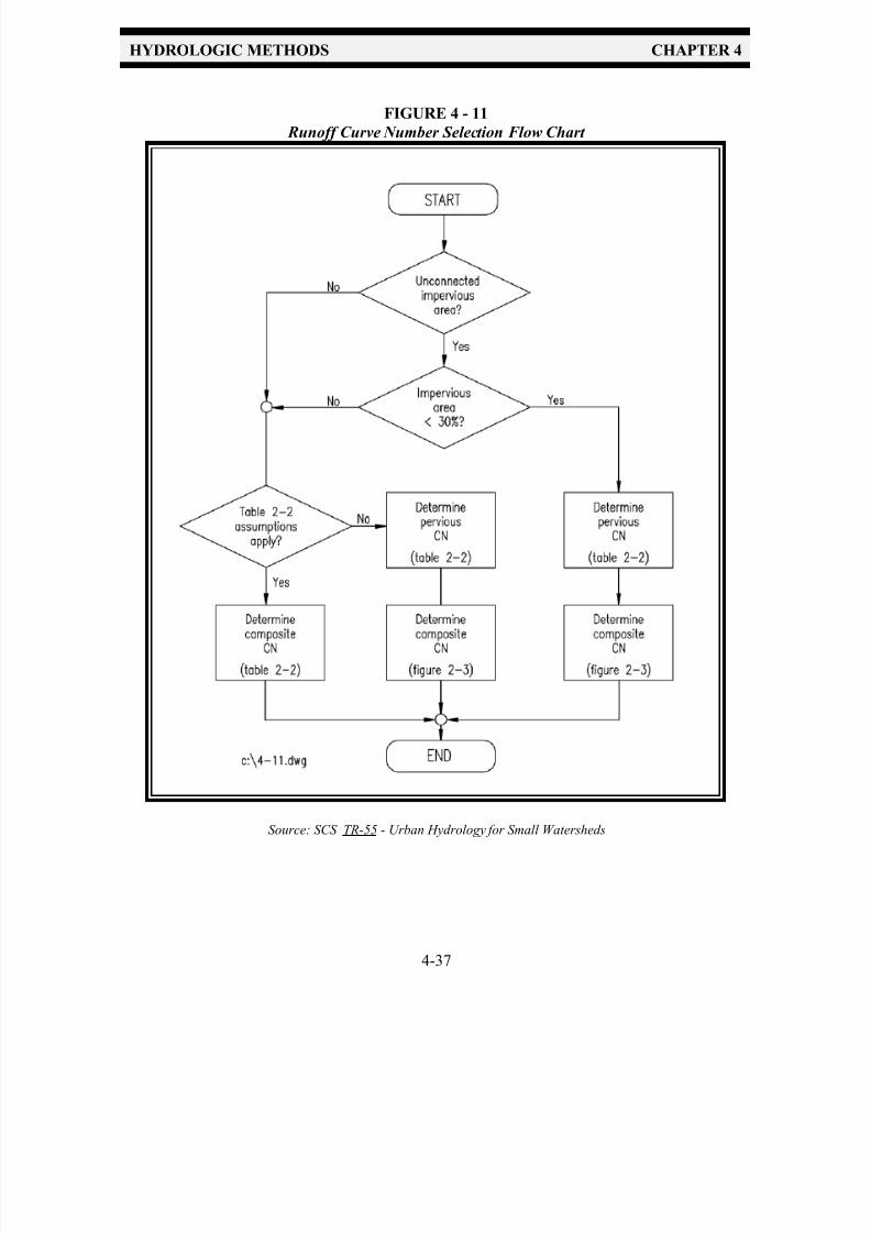
7/30/2019 Virginia Stormwater Managment Handbook Volume_II.pdf
http://slidepdf.com/reader/full/virginia-stormwater-managment-handbook-volumeiipdf 44/354
HYDROLOGIC METHODS CHAPTER 4
4-37
FIGURE 4 - 11
Runoff Curve Number Selection Flow Chart
Source: SCS TR-55 - Urban Hydrology for Small Watersheds
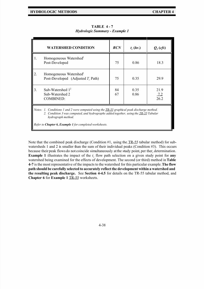
7/30/2019 Virginia Stormwater Managment Handbook Volume_II.pdf
http://slidepdf.com/reader/full/virginia-stormwater-managment-handbook-volumeiipdf 45/354
HYDROLOGIC METHODS CHAPTER 4
4-38
TABLE 4 - 7
Hydrologic Summary - Example 1
WATERSHED CONDITION RCN t c (hr .) Q2 (cfs)
1. Homogeneous Watershed1
Post-Developed 75 0.86 18.3
2. Homogeneous Watershed1
Post-Developed (Adjusted T c Path) 75 0.35 29.9
3. Sub-Watershed 12
Sub-Watershed 2
COMBINED:
84
67
0.35
0.86
21.9
7.2
26.2
Notes: 1. Conditions 1 and 2 were computed using the TR-55 graphical peak discharge method.
2. Condition 3 was computed, and hydrographs added together, using the TR-55 Tabular
hydrograph method.
Refer to Chapter 6, Example 1 for completed worksheets.
Note that the combined peak discharge (Condition #1, using the TR-55 tabular method) for sub-
watersheds 1 and 2 is smaller than the sum of their individual peaks (Condition #3). This occurs
because their peak flows do not coincide simultaneously at the study point, per the t c determination.
Example 1 illustrates the impact of the t c flow path selection on a given study point for any
watershed being examined for the effects of development. The second (or third) method in Table
4-7 is the most representative of the impacts to the watershed for this particular example. The flow
path should be carefully selected to accurately reflect the development within a watershed and
the resulting peak discharge. See Section 4-4.5 for details on the TR-55 tabular method, and
Chapter 6 for Example 1 TR-55 worksheets.

7/30/2019 Virginia Stormwater Managment Handbook Volume_II.pdf
http://slidepdf.com/reader/full/virginia-stormwater-managment-handbook-volumeiipdf 46/354
HYDROLOGIC METHODS CHAPTER 4
4-39
FIGURE 4 - 12
Pre- and Post-Developed Watersheds - Example 1

7/30/2019 Virginia Stormwater Managment Handbook Volume_II.pdf
http://slidepdf.com/reader/full/virginia-stormwater-managment-handbook-volumeiipdf 47/354
HYDROLOGIC METHODS CHAPTER 4
4-40
NOTE: Sheet flow can influence the peak discharge of small watersheds dramatically because
the ratio of flow length to flow velocity is usually very high. Surface roughness, soil types, and
slope will dictate the distance before sheet flow transitions into shallow concentrated flow.
TR-55 stipulates that the maximum length of sheet flow is 300 feet. Many hydrologists and
geologists will argue that, based on the definition of sheet flow, that 100 to 150 feet is the
maximum distance before the combination of quantity and velocity create shallow concentrated
flow. In an urban application (usually a relatively small drainage area), the flow time
associated with 300 feet of sheet flow will result in a disproportionately large segment of the
total time of concentration for the watershed. This will result in a very slow overall t c , and
may not be representative of the drainage area as a whole. As stated previously, the designer must be sure that the flow path chosen is not only representative of the drainage area, but
also is the flow path for the significant portion of the total peak discharge.
2. Flow Segments
The time of concentration is the sum of the time increments for each flow segment present in the t cflow path, such as overland or sheet flow, shallow concentrated flow, and channel flow. These
flow types are influenced by surface roughness, channel shape, flow patterns, and slope, and are
discussed below:
a. Overland (sheet) flow is shallow flow over plane surfaces. For the purposes of determining
time of concentration, overland flow usually exists in the upper reaches of the hydraulic flow
path.
TR-55 utilizes Manning's kinematic solution to compute t c for overland sheet flow. The roughness
coefficient is the primary culprit in the misapplication of the kinematic t c equation. Care should be
taken to accurately identify the surface conditions for overland flow. Table 4-9( a) in this
handbook and Table 3-1 in TR-55 provide selected coefficients for various surface conditions. Refer
to TR-55 and Examples in Chapter 6 for the use of Mannings Kinematic Equation.
Notice that in Example 1, the majority of the pre- and post-developed condition t c flow time for the
watershed is overland sheet flow. Table 4-8 computes the t c for Example 1, (total t c = 0.87 hrs.,
overland sheet flow = 0.75 hrs.) Table 4-8 also shows the sensitivity of the peak discharge to
adjustments in the Manning's roughness coefficient, n, for overland sheet flow. Note that the
manipulation of the roughness coefficient can have a significant impact on the computed discharge.
This illustrates the need for accurate watershed condition data. An on-site investigation should be
completed to determine actual land cover conditions, or the designer should state that assumed
values are being used. Careful selection of the surface roughness coefficient is essential to
calculate an accurate t c and peak discharge.

7/30/2019 Virginia Stormwater Managment Handbook Volume_II.pdf
http://slidepdf.com/reader/full/virginia-stormwater-managment-handbook-volumeiipdf 48/354
HYDROLOGIC METHODS CHAPTER 4
4-41
TABLE 4 - 8
T c and Peak Discharge Sensitivity to Overland Sheet Flow Roughness Coefficient s
DescriptionManning's
‘n’
OverlandSheet Flow
Time*
(hrs.)
Pre-Developed
Total Time of Concentration, t c
(hrs.)
2-Yr. Pre-DevelopedPeak Discharge**
(cfs)
Woods - Light
Underbrush .40 0.75 0.87 8.5
Rangeland-
Natural .13 0.31 0.43 15.0
Woods - DenseUnderbrush
.80 1.31 1.43 6.0
* overland flow time calculated using Manning's kinematic solution (TR-55)
** peak discharge computed using Example 6.1 hydrology
b. Shallow Concentrated Flow usually begins where overland flow converges to form small rills
or gullies. Shallow concentrated flow can exist in small manmade drainage ditches (paved and
unpaved) and in curb and gutters.
TR-55 provides a graphical solution for shallow concentrated flow. The input information needed
to solve for this flow segment is the land slope and the surface condition (paved or unpaved).
c. Channel flow occurs where flow converges in gullies, ditches or swales, and natural or
manmade water conveyances (including storm drainage pipes). Channel flow is assumed to
exist in perennial streams or wherever there is a well-defined channel cross-section.
The Manning Equation is used for open channel flow and pipe flow, and usually assumes full flow
or bank-full velocity. Manning coefficients can be found in Table 4-9(b-d) for open channel flow
(natural and man-made channels) and closed channel flow. Coefficients can also be obtained from
standard textbooks such as Open Channel Hydraulics or Handbook of Hydraulics.

7/30/2019 Virginia Stormwater Managment Handbook Volume_II.pdf
http://slidepdf.com/reader/full/virginia-stormwater-managment-handbook-volumeiipdf 49/354
HYDROLOGIC METHODS CHAPTER 4
4-42
TABLE 4 - 9a
Roughness Coefficient ‘n’ for the Manning Equation - Sheet Flow
Surface Description ‘n’ Value
Smooth Surfaces (Concrete, Asphalt, Gravel, or
Bare Soil . . . . . . . . . . . . . . . . . . . . . . . . . . . . . . . . . . . . . . . . . 0.011
Fallow (No Residue) . . . . . . . . . . . . . . . . . . . . . . . . . . . . . . . . . 0.05
Cultivated Soils:
Residue Cover < 20% . . . . . . . . . . . . . . . . . . . . . . . . . . . . 0.06
Residue Cover > 20% . . . . . . . . . . . . . . . . . . . . . . . . . . . . 0.17
Grass:
Short Grass Prairie . . . . . . . . . . . . . . . . . . . . . . . . . . . . . . 0.15
Dense Grasses2 . . . . . . . . . . . . . . . . . . . . . . . . . . . . . . . . 0.24
Bermuda grass . . . . . . . . . . . . . . . . . . . . . . . . . . . . . . . . . 0.41
Range (Natural) . . . . . . . . . . . . . . . . . . . . . . . . . . . . . . . . . . . . . 0.13
Woods:3
Light Underbrush . . . . . . . . . . . . . . . . . . . . . . . . . . . . . . . 0.40
Dense Underbrush . . . . . . . . . . . . . . . . . . . . . . . . . . . . . . 0.80
1 The ‘n’ values are composite of information compiled by Engman (1986).2 Includes species such as weeping lovegrass, bluegrass, buffalo grass, blue
grama grass, and native grass mixtures.3 When selecting n, consider cover to a height of about 0.1 ft. This is the only part
of the plant cover that will obstruct sheet flow.
From 210-VI-TR-55, Second Edition, June 1986

7/30/2019 Virginia Stormwater Managment Handbook Volume_II.pdf
http://slidepdf.com/reader/full/virginia-stormwater-managment-handbook-volumeiipdf 50/354
HYDROLOGIC METHODS CHAPTER 4
4-43
TABLE 4 - 9b
Roughness Coefficient ‘n’ for the Manning Equation - Pipe Flow
Material
‘n’ Value Range
From To
Coated Cast-iron
Uncoated Cast-iron
Vitrified Sewer Pipe
Concrete Pipe
Common Clay Drainage Tile
Corrugated Metal (2 2/3 x ½)
Corrugated Metal (3 x 1 and 6 x 1)
Corrugated Metal (6 x 2 Structural Plate)
0.010
0.011
0.010
0.010
0.011
0.023
0.026
0.030
0.014
0.015
0.017
0.017
0.017
0.026
0.029
0.033
Source: Handbook of Hydraulics, Sixth Edition, Brater & King
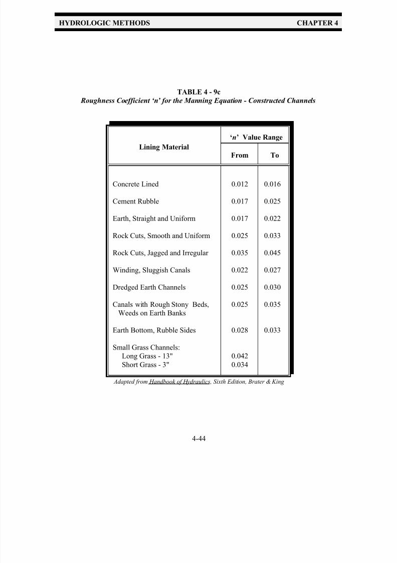
7/30/2019 Virginia Stormwater Managment Handbook Volume_II.pdf
http://slidepdf.com/reader/full/virginia-stormwater-managment-handbook-volumeiipdf 51/354
HYDROLOGIC METHODS CHAPTER 4
4-44
TABLE 4 - 9c Roughness Coefficient ‘n’ for the Manning Equation - Constructed Channels
Lining Material
‘n’ Value Range
From To
Concrete Lined
Cement Rubble
Earth, Straight and Uniform
Rock Cuts, Smooth and Uniform
Rock Cuts, Jagged and Irregular
Winding, Sluggish Canals
Dredged Earth Channels
Canals with Rough Stony Beds,
Weeds on Earth Banks
Earth Bottom, Rubble Sides
Small Grass Channels:
Long Grass - 13"
Short Grass - 3"
0.012
0.017
0.017
0.025
0.035
0.022
0.025
0.025
0.028
0.042
0.034
0.016
0.025
0.022
0.033
0.045
0.027
0.030
0.035
0.033
Adapted from Handbook of Hydraulics, Sixth Edition, Brater & King
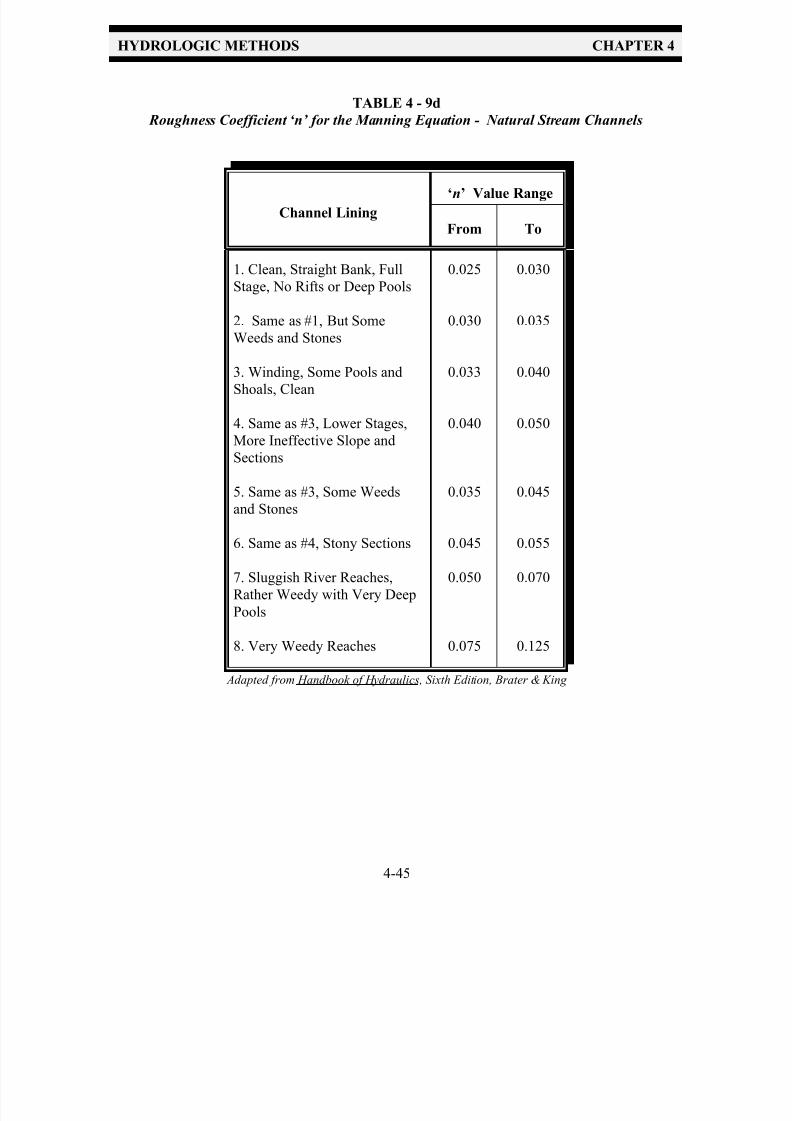
7/30/2019 Virginia Stormwater Managment Handbook Volume_II.pdf
http://slidepdf.com/reader/full/virginia-stormwater-managment-handbook-volumeiipdf 52/354
HYDROLOGIC METHODS CHAPTER 4
4-45
TABLE 4 - 9d
Roughness Coefficient ‘n’ for the Manning Equation - Natural Stream Channels
Channel Lining
‘n’ Value Range
From To
1. Clean, Straight Bank, Full
Stage, No Rifts or Deep Pools
2. Same as #1, But Some
Weeds and Stones
3. Winding, Some Pools andShoals, Clean
4. Same as #3, Lower Stages,
More Ineffective Slope and
Sections
5. Same as #3, Some Weeds
and Stones
6. Same as #4, Stony Sections
7. Sluggish River Reaches,
Rather Weedy with Very Deep
Pools
8. Very Weedy Reaches
0.025
0.030
0.033
0.040
0.035
0.045
0.050
0.075
0.030
0.035
0.040
0.050
0.045
0.055
0.070
0.125
Adapted from Handbook of Hydraulics, Sixth Edition, Brater & King

7/30/2019 Virginia Stormwater Managment Handbook Volume_II.pdf
http://slidepdf.com/reader/full/virginia-stormwater-managment-handbook-volumeiipdf 53/354
HYDROLOGIC METHODS CHAPTER 4
4-46
4-4.4 TR-55 Graphical Peak Discharge Method
The graphical peak discharge method was developed from hydrograph analyses using TR-20,
Computer Program for Project Formulation-Hydrology (SCS, 1983). The graphical method
develops the peak discharge in cubic feet per second(cfs) for a given watershed.
4-4.4.1 Limitations
There are several limitations that the designer should be aware of before using the TR-55 graphical
method:
1. The watershed being studied must be hydrologically homogeneous, i.e., the land use, soils,
and cover are distributed uniformly throughout the watershed and can be described by one
curve number.
2. The watershed may have only one main stream or flow path. If more than one is present they
must have nearly equal t c's so that the entire watershed is represented by one t c .
3. The analysis of the watershed cannot be part of a larger watershed study which would require
adding hydrographs since the graphical method does not generate a hydrograph.
4. For the same reason, the graphical method should not be used if a runoff hydrograph is to be
routed through a control structure.
5. When the initial abstraction - rainfall ratio ( I a / P ) falls outside the range of the Unit Peak
Discharge curves (0.1 to 0.5), the limiting value of the curve must be used.
The reader is encouraged to review the TR-55 Manual to become familiar with these and other limitations associated with the graphical method.
The graphical method can be used as a planning tool to determine the impact of development or land
use changes within a watershed, or to anticipate or predict the need for stormwater management
facilities or conveyance improvements. Sometimes, the graphical method can be used in
conjunction with the TR-55 short-cut method for estimating the storage volume required for post-
developed peak discharge control. This short-cut method is found in Chapter 6 of TR-55 and is
discussed in Chapter 5 of this handbook. However, it should be noted that a more sophisticated
computer model such as TR-20 or HEC-1, or even TR-55 Tabular Hydrograph Method, should be
used for analyzing complex, urbanizing watersheds.

7/30/2019 Virginia Stormwater Managment Handbook Volume_II.pdf
http://slidepdf.com/reader/full/virginia-stormwater-managment-handbook-volumeiipdf 54/354
HYDROLOGIC METHODS CHAPTER 4
4-47
4-4.4.2 Information Needed
The following represents a brief list of the parameters needed to compute the peak discharge of a
watershed using the TR-55 Graphical Peak Discharge Method. For a detailed explanation of the
terms listed, refer to Section 4-4.4.3 in this handbook.
1. The drainage area, in square miles
2. t c , in hours
3. Weighted runoff curve number, CN
4. Rainfall amount, P, for specified design storm, in inches
5. Total runoff, Q, in inches (see runoff equation, TR-55)
6. Initial abstraction, I a , for each subarea
7. Ratio of I a / P for each subarea
8. Rainfall distribution (Type I, IA, II or III)
4-4.4.3 Design Parameters
The TR-55 peak discharge equation is:
q p = qu Am Q F p
Equation 4-3
TR-55 Peak Discharge Equation
where:
q p = peak discharge, cfs
qu = unit peak discharge, cfs/mi2 /in (csm/in)
Am = drainage area, mi2
Q = runoff, in inches, and
F p = pond and swamp adjustment factor
All the required information has been determined earlier except for the unit peak discharge, qu , and
the pond and swamp adjustment factor, F p .
The unit peak discharge, qu , is a function of the initial abstraction, I a , precipitation, P , andthe time of concentration, t c , and can be determined from the Unit Peak Discharge Curves
in TR-55. The unit peak discharge is expressed in cubic feet per second per square mile per
inch of runoff.
Initial abstraction, as indicated previously, is a measure of all the losses that occur before
7/30/2019 Virginia Stormwater Managment Handbook Volume_II.pdf
http://slidepdf.com/reader/full/virginia-stormwater-managment-handbook-volumeiipdf 55/354
HYDROLOGIC METHODS CHAPTER 4
4-48
runoff begins, including infiltration, evaporation, depression storage, and water intercepted
by vegetation, and can be calculated from empirical equations or Table 4-1 in TR-55.
The pond and swamp adjustment factor is an adjustment in the peak discharge to account
for pond and swamp areas if they are spread throughout the watershed and are not considered
in the t c computation. Refer to TR-55 for more information on pond and swamp adjustmentfactors.
The unit peak discharge, qu , is obtained by using t c and the I a /P ratio with Exhibit 4-I, 4-IA, 4-II,
or 4-III (depending on the rainfall distribution type) in TR-55. As limitation number 5 above
indicates, the ratio of I a /P must fall between 0.1 and 0.5. The designer must use the limiting value
on the curves when the computed value is not within this range. The unit peak discharge is
determined from these curves and entered into the above equation to calculate the peak discharge.
4-4.5 TR-55 Tabular Hydrograph Method
The tabular hydrograph method can be used to analyze large heterogeneous watersheds. The
tabular method can develop partial composite flood hydrographs at any point in a watershed by
dividing the watershed into homogeneous subareas. The method is especially applicable for
estimating the effects of land use change in a portion of a watershed.
The tabular hydrograph method provides a tool to efficiently analyze several sub-watersheds to
verify the combined impact at a downstream study point. It is especially useful to verify the timing
of peak discharges. Sometimes, the use of detention in a lower sub-watershed may actually increase
the combined peak discharge at the study point. This procedure allows a quick check to verify the
timing of the peak flows and to decide if a more detailed study is necessary.
4-4.5.1 Limitations
The following represents some of the basic limitations that the designer should be aware of before
using the TR-55 tabular method:
1. The travel time, T t , must be less than 3 hours (largest T t in TR-55 , Exhibit 5).
2. The time of concentration, t c , must be less than 2 hours (largest t c in TR-55 , Exhibit 5).
3. The acreage of the individual sub-watersheds should not differ by a factor of 5 or more.
When these limitations cannot be met, the designer should use the TR-20 computer program or other
available computer models which will provide more accurate and detailed results.
The reader is encouraged to review the TR-55 manual to become familiar with these and other

7/30/2019 Virginia Stormwater Managment Handbook Volume_II.pdf
http://slidepdf.com/reader/full/virginia-stormwater-managment-handbook-volumeiipdf 56/354
HYDROLOGIC METHODS CHAPTER 4
4-49
limitations associated with the tabular method.
4-4.5.2 Information Needed
The following represents a brief list of the parameters needed to compute the peak discharge of a
watershed using the TR-55 Tabular method. For a detailed explanation of the terms listed, refer toSection 4-4.4.3 in this handbook.
1. Subdivision of the watershed into areas that are relatively homogeneous.
2. The drainage area of each subarea, in square miles.
3. Time of concentration, t c , for each subarea in hours.
4. Travel time, T t , for each routing reach, in hours.
5. Weighted runoff curve number, RCN, for each subarea.
6. Rainfall amount, P, in inches, for each specified design storm.7. Total runoff, Q, in inches (see runoff equation, TR-55) for each subarea.
8. Initial abstraction, I a , for each subarea.
9. Ratio of I a /P for each subarea.
10. Rainfall distribution (I, IA, II or III)
4-4.5.3 Design Parameters
The use of the tabular method requires that the designer determine the travel time through the entire
watershed. As stated previously, the entire watershed is divided into smaller sub-watersheds thatmust be related to one another and to the whole watershed with respect to time. The result is that
the time of peak discharge is known for any one sub-watershed relative to any other sub-watershed
or for the entire watershed.
Travel time, T t , represents the time for flow to travel from the study point at the bottom of
a sub-watershed to the bottom of the entire watershed. This information must be compiled
for each sub-watershed.
The data for up to 10 sub-watersheds can be compiled on one TR-55 worksheet. (TR-55 Worksheets
5a and 5b.)
To obtain the peak discharge using the graphical method , the unit peak discharge is read off of a
curve. However, the tabular method provides this information in the form of a table of values, found
in TR-55, Exhibit 5. These tables are arranged by rainfall type (I, IA, II, and III), I a /P , t c , and T t . In most cases, the actual values for these variables, other than the rainfall type, will be different
from the values shown in the table. Therefore, a system of rounding these values has been
7/30/2019 Virginia Stormwater Managment Handbook Volume_II.pdf
http://slidepdf.com/reader/full/virginia-stormwater-managment-handbook-volumeiipdf 57/354
HYDROLOGIC METHODS CHAPTER 4
4-50
The preceding discussion on the Tabular Method is taken from TR-55 and is NOT
complete. The designer should obtain a copy of TR-55 and learn the procedures and
limitations as outlined in that document. Examples and worksheets are provided in
TR-55 that lead the reader through the procedures for each chapter.
established in the TR-55 manual. The I a /P term is simply rounded to the nearest table value. The
t c and T t values are rounded together in a procedure that is outlined on pages 5-2 and 5-3 of the TR-
55 manual. The accuracy of the computed peak discharge and time of peak discharge is highly
dependent on the proper use of these procedures.
The following equation, along with the information compiled on TR-55 Worksheet 5b, is then used
to determine the flow at any time:
q = qt Am Q
Equation 4-4
Tabular Hydrograph Peak Discharge Equation
where: q = hydrograph coordinate in cfs, at hydrograph time t;
qt = tabular hydrograph unit discharge at hydrograph time t from TR-55
Exhibit 5, csm/in;
Am = drainage area of individual subarea, mi2; and
Q = runoff in.
The product AmQ is multiplied by each table value in the appropriate unit hydrograph in TR-55
Exhibit 5, (each sub-watershed may use a different unit hydrograph) to generate the actual
hydrograph for the subwatershed. This hydrograph is tabulated on TR-55 worksheet 5b and then
added together with the hydrographs from the other sub-watersheds, being careful to use the same
time increment for each subwatershed. The result is a composite hydrograph at the bottom of the
worksheet for the entire watershed. Refer to Example 1 in Chapter 6 for a completed analysis using
the TR-55 tabular hydrograph method.

7/30/2019 Virginia Stormwater Managment Handbook Volume_II.pdf
http://slidepdf.com/reader/full/virginia-stormwater-managment-handbook-volumeiipdf 58/354

7/30/2019 Virginia Stormwater Managment Handbook Volume_II.pdf
http://slidepdf.com/reader/full/virginia-stormwater-managment-handbook-volumeiipdf 59/354
CHAPTER 4
APPENDIX

7/30/2019 Virginia Stormwater Managment Handbook Volume_II.pdf
http://slidepdf.com/reader/full/virginia-stormwater-managment-handbook-volumeiipdf 60/354
APPENDIX 4A
Hydrologic Soil Groups in Virginia
The majority of soils found in Virginia along with their corresponding Hydrologic Soil Group
designation are listed on the following pages. All stormwater BMP designs that require specific
soil conditions to be present should be based on an actual soils analysis.

7/30/2019 Virginia Stormwater Managment Handbook Volume_II.pdf
http://slidepdf.com/reader/full/virginia-stormwater-managment-handbook-volumeiipdf 61/354
HYDROLOGIC METHODS APPENDIX
4A - 1
Soil Name Hydgrp Soil Name Hydgrp Soil Name Hydgrp
APPOMATTOX B AQUENTS D AQUULTS D
ARAPAHOE B/D ARCOLA C ARGENT D
ASBURN* C ASHE B ASHLAR B
ASSATEAGUE A ATKINS D ATLEE C
AUGUSTA C AURA B AUSTINVILLE B
AXIS D AYCOCK B BACKBAY D
BADIN B BAILE D BAILEGAP B
BAMA B BAYBORO D BEACHES D
BECKHAM B BELHAVEN D BELTSVILLE C
BELVOIR C BERKS C BERMUDIAN B
BERTIE B BIBB D BILTMORE A
BIRDSBORO B BLADEN D BLAIRTON C
BLAND C BLEAKHILL C BLUEMONT* B
BOHICKET D BOJAC B BOLLING C
BOLTON B BONNEAU A BOOKWOOD B
BOTETOURT C BOURNE C BOWMANSVILLE B/D
BRADDOCK B BRADLEY C BRANDYWINE C
BRECKNOCK B BREMO C BRENTSVILLE C
BROADWAY B BROCKROAD C BRUSHY B
BUCHANAN C BUCKHALL B BUCKS B
BUCKTON B BUFFSTAT B BUGLEY C/D
BUNCOMBE A BURKETOWN C BURROWSVILLE C
CALVERTON C CALVIN C CAMOCCA A/D
CANEYVILLE C CARBO C CARDIFF B
CAROLINE C CARRVALE D CARTECAY C
CATASKA D CATHARPIN C CATLETT C/D
CATOCTIN C CATPOINT A CAVERNS B
CECIL B CHAGRIN B CHAPANOKE C
7/30/2019 Virginia Stormwater Managment Handbook Volume_II.pdf
http://slidepdf.com/reader/full/virginia-stormwater-managment-handbook-volumeiipdf 62/354
HYDROLOGIC METHODS APPENDIX
4A - 2
Soil Name Hydgrp Soil Name Hydgrp Soil Name Hydgrp
CHASTAIN D CHATUGE D CHAVIES B
CHENNEBY C CHESTER B CHEWACLA C
CHICKAHOMINY D CHILHOWIE C CHINCOTEAGUE D
CHIPLEY C CHISWELL D CHRISTIAN C
CID C CLAPHAM* C CLEARBROOK D
CLIFTON C CLUBCAF D CLYMER D
COASTAL BEACH D CODORUS C COLFAX C
COLLEEN C COLVARD B COMBS B
COMUS B CONETOE A CONGAREE B
COOSAW B COROLLA D CORYDON D
COTACO C COURSEY C COWEE B
COXVILLE D CRAIGSVILLE B CRAVEN C
CREEDMOOR C CROTON D CULLEN C
CULPEPER C DALEVILLE D DANDRIDGE D
DAVIDSON B DAWHOO VARIANT B/D DECATUR B
DEKALB C DELANCO C DELOSS B/D
DERROC B DILLARD C DOGUE C
DOROVAN D DOTHAN B DRAGSTON C
DRALL B DRYPOND D DUCKSTON A/D
DUFFIELD B DULLES D DUMFRIES B
DUNBAR D DUNNING D DUPLIN C
DURHAM B DYKE B EBBING C
EDGEHILL C EDNEDYTOWN B EDNEYVILLE B
EDOM C ELBERT D ELIOAK C
ELSINBORO B EMPORIA C ENDCAV C
ELIOK C ELKTON C/D ELLIBER A
7/30/2019 Virginia Stormwater Managment Handbook Volume_II.pdf
http://slidepdf.com/reader/full/virginia-stormwater-managment-handbook-volumeiipdf 63/354
HYDROLOGIC METHODS APPENDIX
4A - 3
Soil Name Hydgrp Soil Name Hydgrp Soil Name Hydgrp
ENON C ENOTT C ERNEST C
EUBANKS B EULONIA C EUNOLA C
EVANSHAM D EVARD B EVERGREEN B
EXUM C FACEVILLE B FAIRFAX B
FALLSINGTON B/D FAUGUIER C FAYWOOD C
FEATHERSTONE D FISHERMAN D FLATWOODS C
FLETCHER B FLUVANNA C FLUVAQUENTS D
FORESTDALE D FORK C FRANKSTOWN B
FREDERICK B FRENCH C FRIPP A
GAILA B GAINESBORO C GALESTOWN A
GEORGEVILLE B GILPIN C GLADEHILL B
GLENELG B GLENVILLE C GLENWOOD B
GOLDSBORO B GOLDSTON C GOLDVEIN C
GORESVILLE* B GREENLEE B GRIMSLEY B
GRITNEY C GROSECLOSE C GROVER B
GUERNSEY C GULLION C GUNSTOCK C
GUYAN C GWINNETT VARIENT B HAGERSTOWN C
HALEWOOD B HARTLETON B HATBORO D
HAWKSBILL B HAYESVILLE B HAYMARKET D
HAYTER B HAYWOOD B HAZEL C
HAZEL CHANNERY C HAZELTON B HELENA C
HERNDON B HIWASSEE B HOADLY C
HOBUCKEN D HOGELAND* C HOLLYWOOD D
HUNTINGTON B HYATTSVILLE B HYDE B/D
HYDRAQUENTS B INGLEDOVE B IREDELL C/D

7/30/2019 Virginia Stormwater Managment Handbook Volume_II.pdf
http://slidepdf.com/reader/full/virginia-stormwater-managment-handbook-volumeiipdf 64/354
HYDROLOGIC METHODS APPENDIX
4A - 4
Soil Name Hydgrp Soil Name Hydgrp Soil Name Hydgrp
IRONGATE B IUKA C IZAGORA C
JACKLAND D JEDBURG C JEFFERSON B
JOHNS C JOHNSTON D JUNALUSKA B
KALMIA B KELLY D KEMPSVILLE B
KENANSVILLE A KENANSVILLE
VARIANT
C KEYPORT C
KINKORA D KINSTON B/D KLEJ B
KLINESVILLE C/D KONNAROCK C LAIDIG C
LAKEHURSTVARIANT
A LAKELAND A LANEXA D
LANSDALE B LAROQUE B LAWNES D
LEAF D LEAKSVILLE D LECK KILL B
LEEDSVILLE* B LEETONIA C LEGORE B
LEHEW C LENOIR D LEON B/D
LEVY D LEW B LEWISBERRY B
LIBRARY D LIGNUM C LILY B
LINDSIDE C LITTLEJOE B LITZ C
LLOYD C LOBDELL B LODI B
LOUISA B LOUISBURG B LOWELL C
LUCKETTS B LUCY A LUGNUM C
LUMBEE B/D LUNT C LYNCHBURG C
MACOVE B MADISON B MAGOTHA D
MANASSAS B MANOR B MANTACHIE C
MANTEO C/D MARBIE C MARGO B
MARLBORO B MARR B MARUMSCO C
MASADA C MASSANETTA B MASSANUTTEN B
MATAPEAKE B MATNELFLAT B MATTAN D

7/30/2019 Virginia Stormwater Managment Handbook Volume_II.pdf
http://slidepdf.com/reader/full/virginia-stormwater-managment-handbook-volumeiipdf 65/354
HYDROLOGIC METHODS APPENDIX
4A - 5
Soil Name Hydgrp Soil Name Hydgrp Soil Name Hydgrp
MATTAPEX C MATTAPONI C MAURERTOWN D
MAYODAN B MCGARY C MCQUEEN C
MEADOWS D MEADOWVILLE B MECKLENBURG C
MEGGETT D MELFA D MELVIN D
MILLROCK A MINNIEVILLE C MIXED ALLUVIUM D
MOLENA A MONACAN C MONGLE C
MONONGAHELA C MONTALTO C MONTRESSOR* B
MONTROSS C MOOMAW C MORRISONVILLE* B
MORVEN B MOUNT LUCAS C MT WEATHER* B
MUCKALEE D MUNDEN B MURRILL B
MYATT D MYATT VARIANT D MYERSVILLE B
NAHUNTA C NANSEMOND C NASON B
NAWNEY D NEABSCO C NESTORIA C/D
NEVARC C NEWARK C NEWBERN C
NEWFLAT D NEWHAN A NEWMARC C
NICHOLOSON C NI MMO D NIXA C
NOLICHUCKY B NOLIN B NOMERVILLE B
NORFOLK B OAKHILL B OAKLET C
OATLANDS B OCCOQUAN B OCHLOCKONEE B
OKEETEE D OPEQUON C ORANGE D
ORANGEBURG B ORENDA B ORISKANY B
OSIER A/D OTHELLO C/D PACOLET B
PACTOLUS A PAGEBROOK D PAMLICO D
PAMUNKEY B PAMUNKEY
VARIANT
A PANORAMA B
PARKER B PARTLOW D PASQUOTANK B/D
PEAKS C PEAWICK D PENN C/D
7/30/2019 Virginia Stormwater Managment Handbook Volume_II.pdf
http://slidepdf.com/reader/full/virginia-stormwater-managment-handbook-volumeiipdf 66/354
HYDROLOGIC METHODS APPENDIX
4A - 6
Soil Name Hydgrp Soil Name Hydgrp Soil Name Hydgrp
PHILO B PHILOMOMT* B PINEYWOODS D
PINKSTON B PISGAH C POCATY D
POCOMOKE B/D POINDEXTER B POLAWANA A/D
POOLER VARIANT D POPE B POPLIMENTO C
PORTERS B PORTSMOUTH B/D POUNCEY D
PUNGO D PURCELLVILLE B PURDY D
RABUM B RAINS B/D RAMSEY D
RAPIDAN B RAPPHANNOCK D RARITAN C
RAYNE B READINGTON C REAVILLE C
REMLIK A RIGLEY B RION B
RIVERVIEW B ROANOKE D ROHRERSVILLE D
ROSS B ROWLAND C RUMFORD B
RUSHTOWN A RUSTON B SAFELL B
SASSAFRAS B SASSAFRAS B SAUNOOK B
SAVANNAH C SCATTERSVILLE* C SCHAFFENAKER A
SEABROOK C SEDGEFIELD C SEKIL B
SENECA B SEQUOIA C SHELOCTA B
SHENVAL B SHERANDO B SHEVA C
SHOTTOWER B SINDION B SKETERVILLE C
SLABTOWN B SLAGLE C SLICKENS B
SNICKERSVILLE B SPEEDWELL B SPESSARD A
SPIVEY B SPOSTSYLVANIA C SPRIGGS C
SPRINGWOOD B STANTON D STARR C
STATE B STEINSBURG C STONEVILLE B
STUART C STUMPTOWN B SUCHES B
SUDLEY B SUEQUEHANNA D SUFFOLK B
SUSDLEY B SUSQUEHANNA D SWAMP D
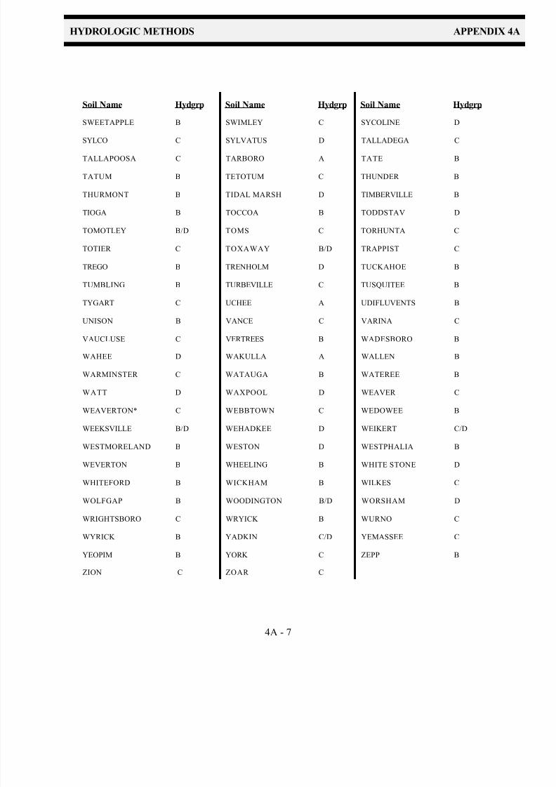
7/30/2019 Virginia Stormwater Managment Handbook Volume_II.pdf
http://slidepdf.com/reader/full/virginia-stormwater-managment-handbook-volumeiipdf 67/354
HYDROLOGIC METHODS APPENDIX
4A - 7
Soil Name Hydgrp Soil Name Hydgrp Soil Name Hydgrp
SWEETAPPLE B SWIMLEY C SYCOLINE D
SYLCO C SYLVATUS D TALLADEGA C
TALLAPOOSA C TARBORO A TATE B
TATUM B TETOTUM C THUNDER B
THURMONT B TIDAL MARSH D TIMBERVILLE B
TIOGA B TOCCOA B TODDSTAV D
TOMOTLEY B/D TOMS C TORHUNTA C
TOTIER C TOXAWAY B/D TRAPPIST C
TREGO B TRENHOLM D TUCKAHOE B
TUMBLING B TURBEVILLE C TUSQUITEE B
TYGART C UCHEE A UDIFLUVENTS B
UNISON B VANCE C VARINA C
VAUCLUSE C VERTREES B WADESBORO B
WAHEE D WAKULLA A WALLEN B
WARMINSTER C WATAUGA B WATEREE B
WATT D WAXPOOL D WEAVER C
WEAVERTON* C WEBBTOWN C WEDOWEE B
WEEKSVILLE B/D WEHADKEE D WEIKERT C/D
WESTMORELAND B WESTON D WESTPHALIA B
WEVERTON B WHEELING B WHITE STONE D
WHITEFORD B WICKHAM B WILKES C
WOLFGAP B WOODINGTON B/D WORSHAM D
WRIGHTSBORO C WRYICK B WURNO C
WYRICK B YADKIN C/D YEMASSEE C
YEOPIM B YORK C ZEPP B
ZION C ZOAR C

7/30/2019 Virginia Stormwater Managment Handbook Volume_II.pdf
http://slidepdf.com/reader/full/virginia-stormwater-managment-handbook-volumeiipdf 68/354
APPENDIX 4B
24-hour Rainfall Data for Virginia
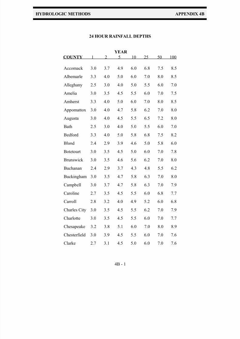
7/30/2019 Virginia Stormwater Managment Handbook Volume_II.pdf
http://slidepdf.com/reader/full/virginia-stormwater-managment-handbook-volumeiipdf 69/354
HYDROLOGIC METHODS APPENDIX 4B
4B - 1
Accomack 3.0 3.7 4.9 6.0 6.8 7.5 8.5
Albemarle 3.3 4.0 5.0 6.0 7.0 8.0 8.5
Alleghany 2.5 3.0 4.0 5.0 5.5 6.0 7.0
Amelia 3.0 3.5 4.5 5.5 6.0 7.0 7.5
Amherst 3.3 4.0 5.0 6.0 7.0 8.0 8.5
Appomattox 3.0 4.0 4.7 5.8 6.2 7.0 8.0
Augusta 3.0 4.0 4.5 5.5 6.5 7.2 8.0
Bath 2.5 3.0 4.0 5.0 5.5 6.0 7.0
Bedford 3.3 4.0 5.0 5.8 6.8 7.5 8.2
Bland 2.4 2.9 3.9 4.6 5.0 5.8 6.0
Botetourt 3.0 3.5 4.5 5.0 6.0 7.0 7.8
Brunswick 3.0 3.5 4.6 5.6 6.2 7.0 8.0
Buchanan 2.4 2.9 3.7 4.3 4.8 5.5 6.2
Buckingham 3.0 3.5 4.7 5.8 6.3 7.0 8.0
Campbell 3.0 3.7 4.7 5.8 6.3 7.0 7.9
Caroline 2.7 3.5 4.5 5.5 6.0 6.8 7.7
Carroll 2.8 3.2 4.0 4.9 5.2 6.0 6.8
Charles City 3.0 3.5 4.5 5.5 6.2 7.0 7.9
Charlotte 3.0 3.5 4.5 5.5 6.0 7.0 7.7
Chesapeake 3.2 3.8 5.1 6.0 7.0 8.0 8.9
Chesterfield 3.0 3.9 4.5 5.5 6.0 7.0 7.6
Clarke 2.7 3.1 4.5 5.0 6.0 7.0 7.6
24 HOUR RAINFALL DEPTHS
YEAR
COUNTY 1 2 5 10 25 50 100
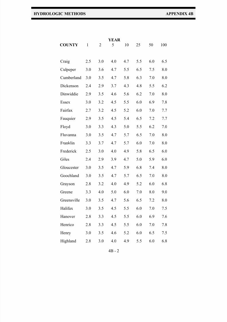
7/30/2019 Virginia Stormwater Managment Handbook Volume_II.pdf
http://slidepdf.com/reader/full/virginia-stormwater-managment-handbook-volumeiipdf 70/354
HYDROLOGIC METHODS APPENDIX 4B
4B - 2
Craig 2.5 3.0 4.0 4.7 5.5 6.0 6.5
Culpeper 3.0 3.6 4.7 5.5 6.5 7.5 8.0
Cumberland 3.0 3.5 4.7 5.8 6.3 7.0 8.0
Dickenson 2.4 2.9 3.7 4.3 4.8 5.5 6.2
Dinwiddie 2.9 3.5 4.6 5.6 6.2 7.0 8.0
Essex 3.0 3.2 4.5 5.5 6.0 6.9 7.8
Fairfax 2.7 3.2 4.5 5.2 6.0 7.0 7.7
Fauquier 2.9 3.5 4.5 5.4 6.5 7.2 7.7
Floyd 3.0 3.3 4.3 5.0 5.5 6.2 7.0
Fluvanna 3.0 3.5 4.7 5.7 6.5 7.0 8.0
Franklin 3.3 3.7 4.7 5.7 6.0 7.0 8.0
Frederick 2.5 3.0 4.0 4.9 5.8 6.5 6.0
Giles 2.4 2.9 3.9 4.7 5.0 5.9 6.0Gloucester 3.0 3.5 4.7 5.9 6.8 7.4 8.0
Goochland 3.0 3.5 4.7 5.7 6.5 7.0 8.0
Grayson 2.8 3.2 4.0 4.9 5.2 6.0 6.8
Greene 3.3 4.0 5.0 6.0 7.0 8.0 9.0
Greensville 3.0 3.5 4.7 5.6 6.5 7.2 8.0
Halifax 3.0 3.5 4.5 5.5 6.0 7.0 7.5
Hanover 2.8 3.3 4.5 5.5 6.0 6.9 7.6
Henrico 2.8 3.3 4.5 5.5 6.0 7.0 7.8
Henry 3.0 3.5 4.6 5.2 6.0 6.5 7.5
Highland 2.8 3.0 4.0 4.9 5.5 6.0 6.8
YEAR
COUNTY 1 2 5 10 25 50 100

7/30/2019 Virginia Stormwater Managment Handbook Volume_II.pdf
http://slidepdf.com/reader/full/virginia-stormwater-managment-handbook-volumeiipdf 71/354
HYDROLOGIC METHODS APPENDIX 4B
4B - 3
YEAR
COUNTY 1 2 5 10 25 50 100
Isle of Wight 2.9 3.7 5.0 5.8 6.6 7.5 8.4
James City 2.8 3.5 4.7 5.8 6.4 7.2 8.0
King and Queen 2.8 3.4 4.5 5.7 6.2 7.0 7.9
King George 2.8 3.2 4.5 5.5 6.0 7.0 7.5
King William 2.8 3.4 4.5 5.7 6.2 7.0 7.9
Lancaster 2.8 3.5 4.7 5.7 6.5 7.2 8.0
Lee 2.7 3.0 3.7 4.5 5.0 5.6 6.0
Loudoun 3.0 3.3 4.5 5.2 6.0 6.9 7.5
Louisa 2.9 3.5 4.7 5.5 6.0 7.0 8.0
Lunenburg 2.9 3.5 4.5 5.5 6.0 7.0 7.5
Madison 3.3 4.0 5.0 6.0 7.0 8.0 9.0
Mathews 3.0 3.6 4.8 5.8 6.6 7.2 8.1
Mecklenburg 2.9 3.5 4.5 5.5 6.0 7.0 7.8
Middlesex 3.0 3.5 4.7 5.7 6.5 7.0 8.0
Montgomery 2.5 3.0 4.0 5.0 5.5 6.0 7.0
Nelson 3.3 4.0 5.0 6.0 7.0 8.0 8.5
New Kent 2.8 3.5 4.5 5.6 6.2 7.0 7.9
Northampton 3.1 3.7 5.0 6.0 6.8 7.6 8.6
Northumberland 2.8 3.5 4.7 5.7 6.5 7.2 8.0
Nottoway 3.0 3.5 4.5 5.5 6.0 7.0 7.9
Orange 3.2 3.5 4.7 5.5 6.5 7.5 8.0
Page 2.5 3.2 4.7 5.5 7.0 7.5 8.5
Patrick 2.8 3.5 4.5 5.0 5.8 6.2 7.3

7/30/2019 Virginia Stormwater Managment Handbook Volume_II.pdf
http://slidepdf.com/reader/full/virginia-stormwater-managment-handbook-volumeiipdf 72/354
HYDROLOGIC METHODS APPENDIX 4B
4B - 4
Pittsylvania 2.8 3.5 4.5 5.2 6.2 6.7 7.5
Powhatan 3.0 3.5 4.5 5.5 6.0 7.0 7.5
Prince Edward 3.0 3.5 4.5 5.5 6.0 7.0 7.8
Prince George 3.0 3.5 4.7 5.7 6.2 7.0 8.0
Prince William 3.0 3.5 4.S 5.3 6.0 7.0 7.8
Pulaski 2.5 3.0 4.0 4.8 5.0 6.0 6.5
Rappahannock 3.0 4.0 4.7 5.7 7.0 8.0 8.5
Richmond 3.0 3.5 4.5 5.7 6.2 7.0 7.9
Roanoke 3.0 3.5 4.5 5.0 6.0 6.7 7.5
Rockbridge 3.0 3.5 4.5 5.5 6.2 7.0 8.0
Rockingham 3.0 3.5 4.5 5.0 6.0 7.0 8.0
Russell 2.5 3.0 3.8 4.4 5.0 5.5 6.0
Scott 2.6 3.0 3.7 4.5 5.0 5.5 6.0
Shenandoah 2.5 3.0 4.0 5.0 6.0 6.5 7.0
Smyth 2.6 2.9 3.8 4.5 5.0 5.6 6.0
Southampton 2.8 3.4 4.8 5.7 6.5 7.2 8.0
Spotsylvania 3.1 3.5 4.5 5.5 6.0 7.0 7.5
Stafford 2.9 3.5 4.5 5.5 6.0 7.0 7.5
Suffolk 3.2 3.7 5.0 6.0 6.7 7.7 8.5
Surry 2.8 3.4 4.8 5.7 6.5 7.2 8.0
Sussex 2.8 3.4 4.8 5.7 6.5 7.2 8.0
Tazewell 2.5 2.9 3.8 4.4 5.0 5.5 6.0
Virginia Beach 3.0 3.8 5.0 6.0 7.0 8.0 9.0
YEAR
COUNTY 1 2 5 10 25 50 100
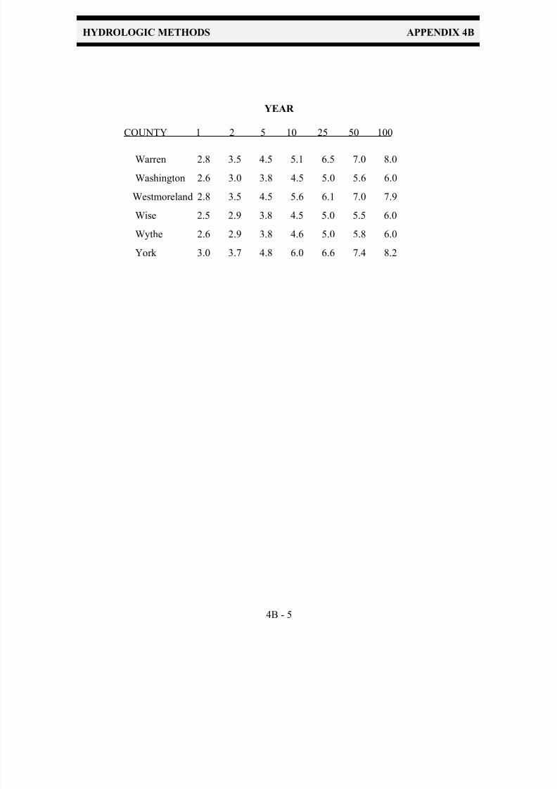
7/30/2019 Virginia Stormwater Managment Handbook Volume_II.pdf
http://slidepdf.com/reader/full/virginia-stormwater-managment-handbook-volumeiipdf 73/354
HYDROLOGIC METHODS APPENDIX 4B
4B - 5
Warren 2.8 3.5 4.5 5.1 6.5 7.0 8.0
Washington 2.6 3.0 3.8 4.5 5.0 5.6 6.0
Westmoreland 2.8 3.5 4.5 5.6 6.1 7.0 7.9
Wise 2.5 2.9 3.8 4.5 5.0 5.5 6.0
Wythe 2.6 2.9 3.8 4.6 5.0 5.8 6.0
York 3.0 3.7 4.8 6.0 6.6 7.4 8.2
YEAR
COUNTY 1 2 5 10 25 50 100

7/30/2019 Virginia Stormwater Managment Handbook Volume_II.pdf
http://slidepdf.com/reader/full/virginia-stormwater-managment-handbook-volumeiipdf 74/354
APPENDIX 4C
Tabular Listing of Runoff Depths for Curve Numbers

7/30/2019 Virginia Stormwater Managment Handbook Volume_II.pdf
http://slidepdf.com/reader/full/virginia-stormwater-managment-handbook-volumeiipdf 75/354

7/30/2019 Virginia Stormwater Managment Handbook Volume_II.pdf
http://slidepdf.com/reader/full/virginia-stormwater-managment-handbook-volumeiipdf 76/354

7/30/2019 Virginia Stormwater Managment Handbook Volume_II.pdf
http://slidepdf.com/reader/full/virginia-stormwater-managment-handbook-volumeiipdf 77/354
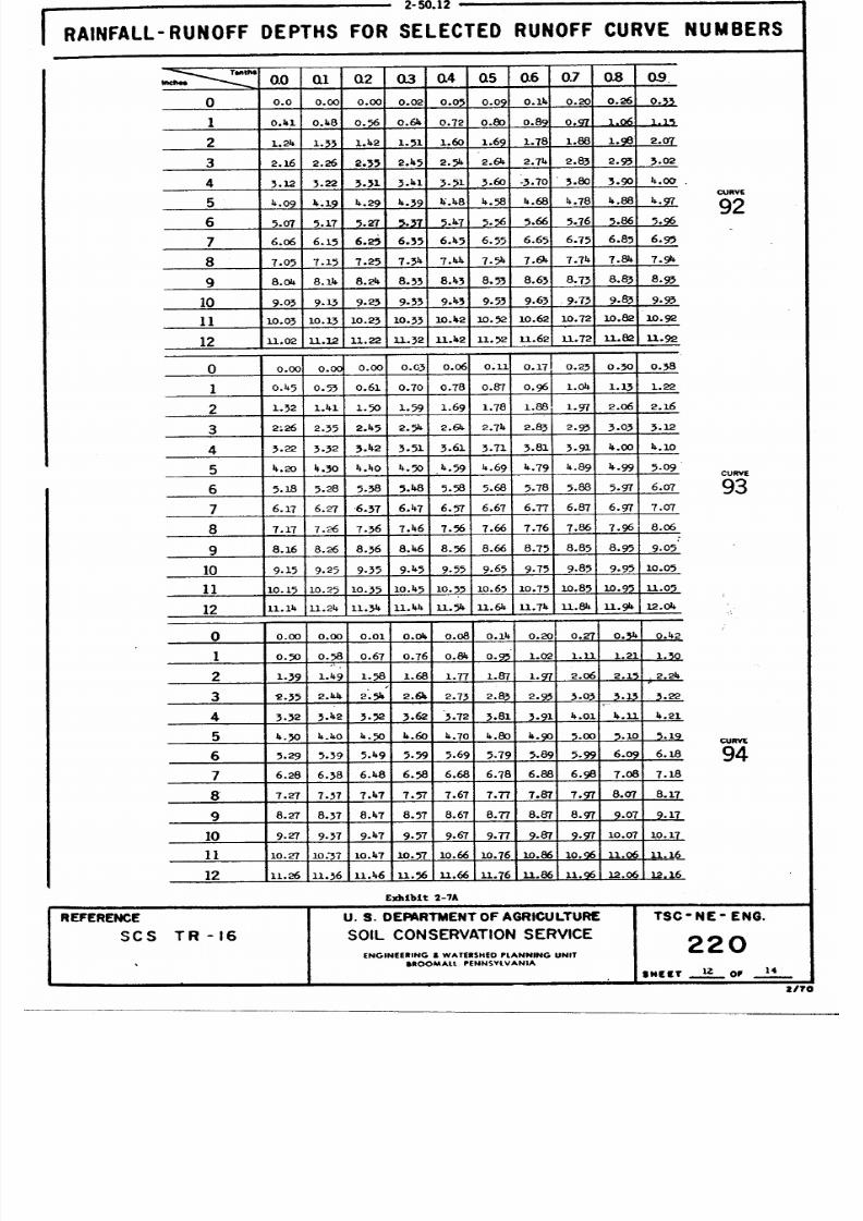
7/30/2019 Virginia Stormwater Managment Handbook Volume_II.pdf
http://slidepdf.com/reader/full/virginia-stormwater-managment-handbook-volumeiipdf 78/354

7/30/2019 Virginia Stormwater Managment Handbook Volume_II.pdf
http://slidepdf.com/reader/full/virginia-stormwater-managment-handbook-volumeiipdf 79/354

7/30/2019 Virginia Stormwater Managment Handbook Volume_II.pdf
http://slidepdf.com/reader/full/virginia-stormwater-managment-handbook-volumeiipdf 80/354

7/30/2019 Virginia Stormwater Managment Handbook Volume_II.pdf
http://slidepdf.com/reader/full/virginia-stormwater-managment-handbook-volumeiipdf 81/354

7/30/2019 Virginia Stormwater Managment Handbook Volume_II.pdf
http://slidepdf.com/reader/full/virginia-stormwater-managment-handbook-volumeiipdf 82/354

7/30/2019 Virginia Stormwater Managment Handbook Volume_II.pdf
http://slidepdf.com/reader/full/virginia-stormwater-managment-handbook-volumeiipdf 83/354
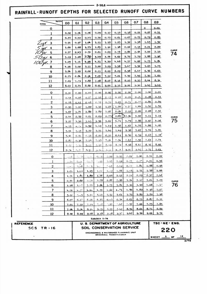
7/30/2019 Virginia Stormwater Managment Handbook Volume_II.pdf
http://slidepdf.com/reader/full/virginia-stormwater-managment-handbook-volumeiipdf 84/354

7/30/2019 Virginia Stormwater Managment Handbook Volume_II.pdf
http://slidepdf.com/reader/full/virginia-stormwater-managment-handbook-volumeiipdf 85/354

7/30/2019 Virginia Stormwater Managment Handbook Volume_II.pdf
http://slidepdf.com/reader/full/virginia-stormwater-managment-handbook-volumeiipdf 86/354

7/30/2019 Virginia Stormwater Managment Handbook Volume_II.pdf
http://slidepdf.com/reader/full/virginia-stormwater-managment-handbook-volumeiipdf 87/354
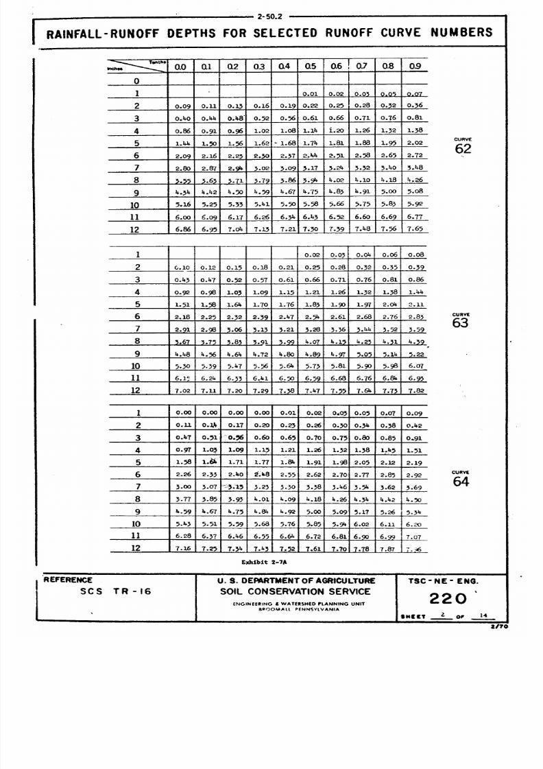
7/30/2019 Virginia Stormwater Managment Handbook Volume_II.pdf
http://slidepdf.com/reader/full/virginia-stormwater-managment-handbook-volumeiipdf 88/354
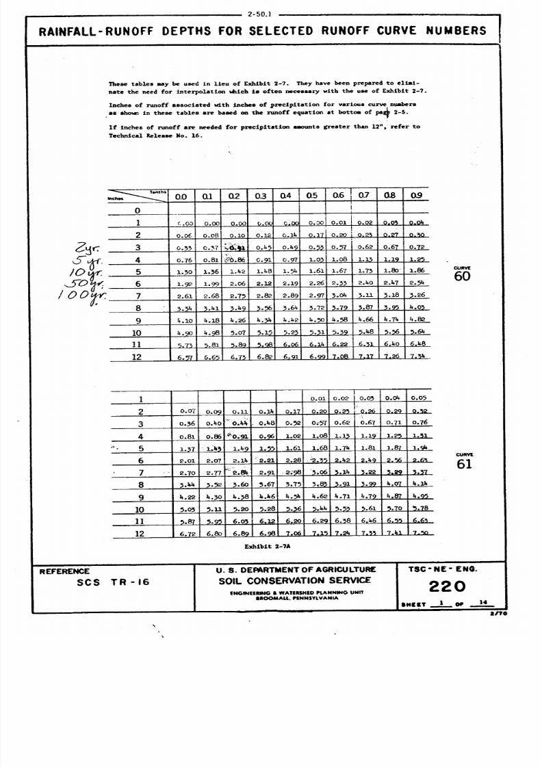
7/30/2019 Virginia Stormwater Managment Handbook Volume_II.pdf
http://slidepdf.com/reader/full/virginia-stormwater-managment-handbook-volumeiipdf 89/354
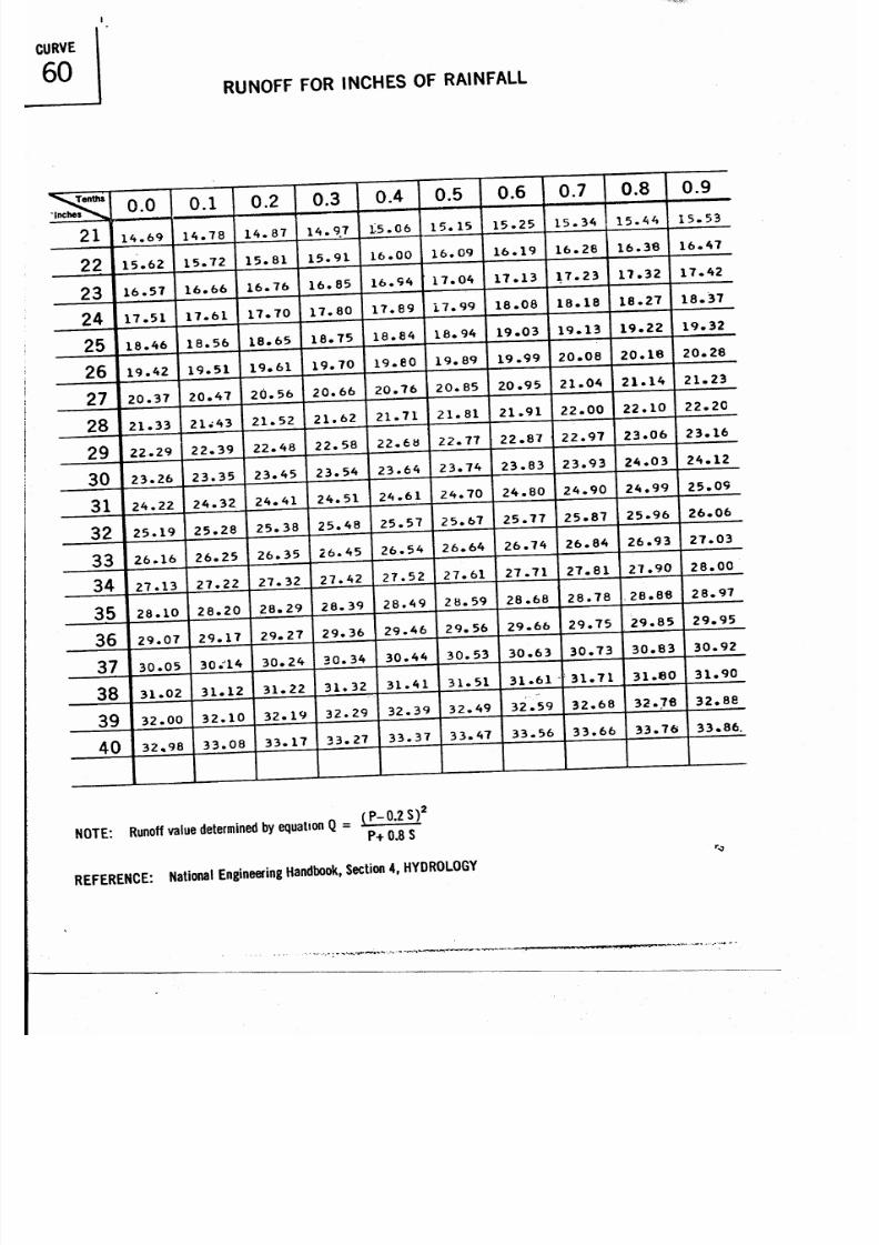
7/30/2019 Virginia Stormwater Managment Handbook Volume_II.pdf
http://slidepdf.com/reader/full/virginia-stormwater-managment-handbook-volumeiipdf 90/354

7/30/2019 Virginia Stormwater Managment Handbook Volume_II.pdf
http://slidepdf.com/reader/full/virginia-stormwater-managment-handbook-volumeiipdf 91/354

7/30/2019 Virginia Stormwater Managment Handbook Volume_II.pdf
http://slidepdf.com/reader/full/virginia-stormwater-managment-handbook-volumeiipdf 92/354
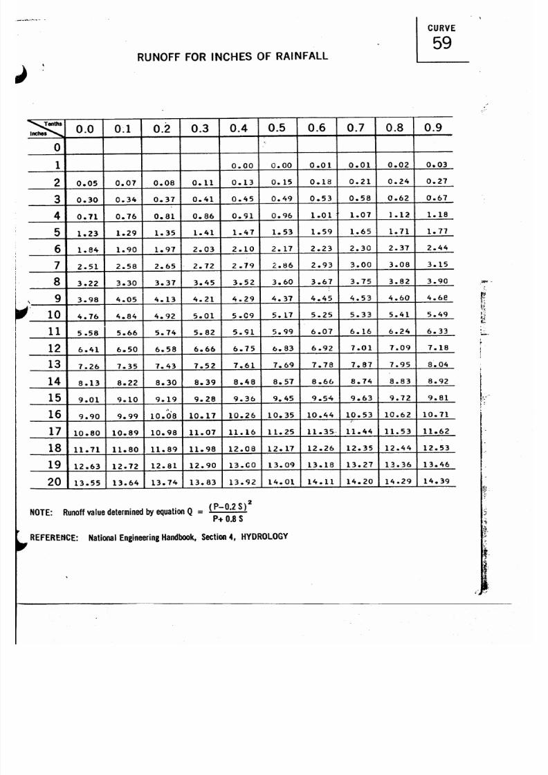
7/30/2019 Virginia Stormwater Managment Handbook Volume_II.pdf
http://slidepdf.com/reader/full/virginia-stormwater-managment-handbook-volumeiipdf 93/354
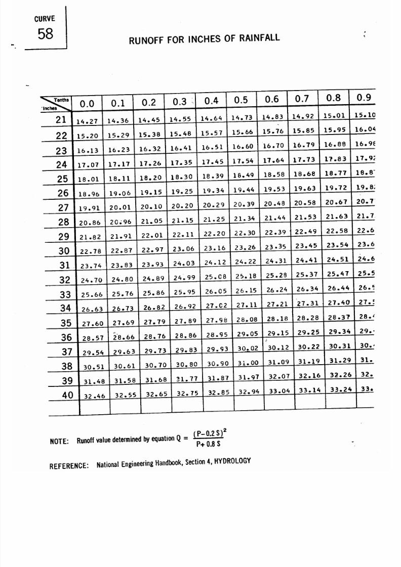
7/30/2019 Virginia Stormwater Managment Handbook Volume_II.pdf
http://slidepdf.com/reader/full/virginia-stormwater-managment-handbook-volumeiipdf 94/354
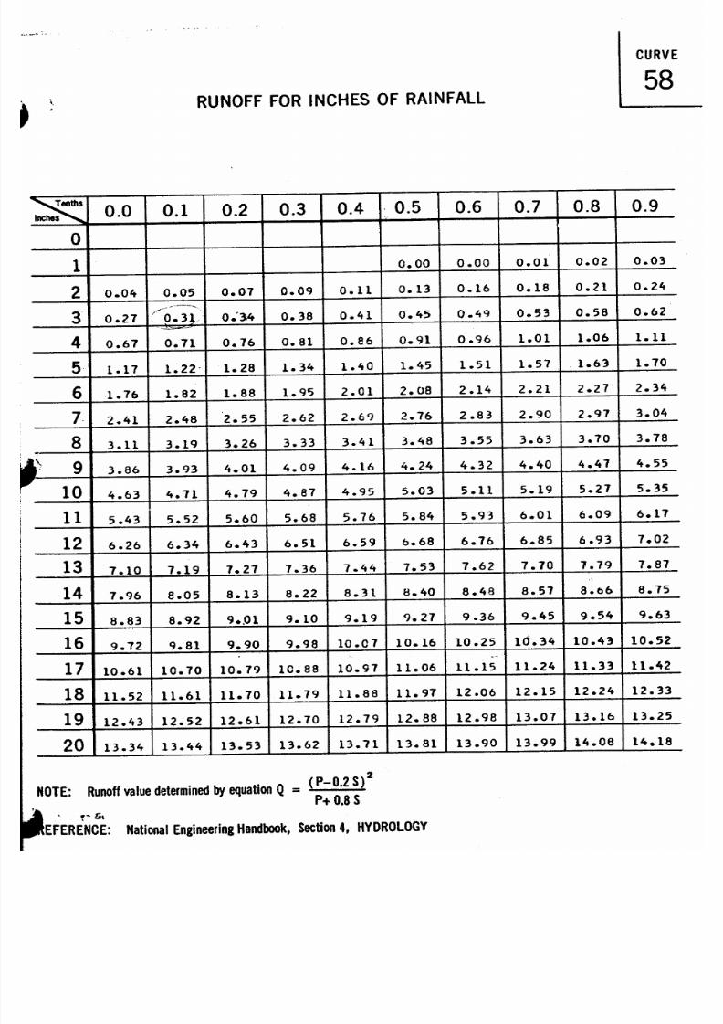
7/30/2019 Virginia Stormwater Managment Handbook Volume_II.pdf
http://slidepdf.com/reader/full/virginia-stormwater-managment-handbook-volumeiipdf 95/354
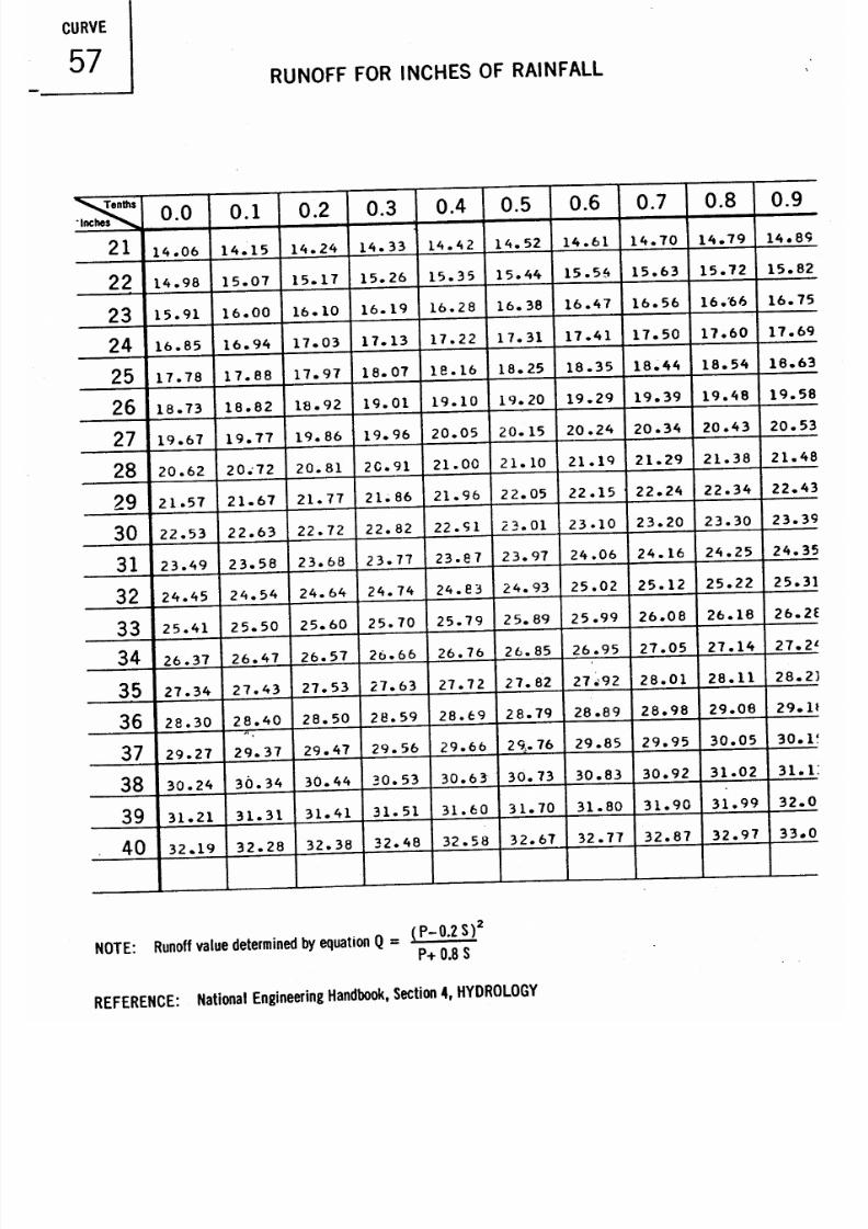
7/30/2019 Virginia Stormwater Managment Handbook Volume_II.pdf
http://slidepdf.com/reader/full/virginia-stormwater-managment-handbook-volumeiipdf 96/354
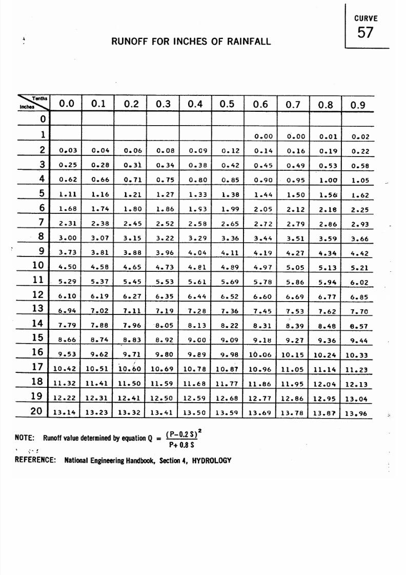
7/30/2019 Virginia Stormwater Managment Handbook Volume_II.pdf
http://slidepdf.com/reader/full/virginia-stormwater-managment-handbook-volumeiipdf 97/354

7/30/2019 Virginia Stormwater Managment Handbook Volume_II.pdf
http://slidepdf.com/reader/full/virginia-stormwater-managment-handbook-volumeiipdf 98/354

7/30/2019 Virginia Stormwater Managment Handbook Volume_II.pdf
http://slidepdf.com/reader/full/virginia-stormwater-managment-handbook-volumeiipdf 99/354
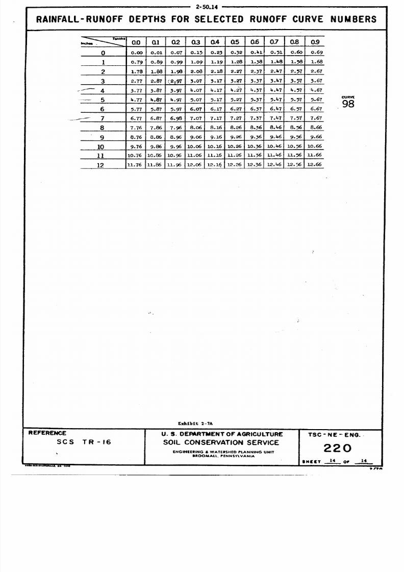
7/30/2019 Virginia Stormwater Managment Handbook Volume_II.pdf
http://slidepdf.com/reader/full/virginia-stormwater-managment-handbook-volumeiipdf 100/354

7/30/2019 Virginia Stormwater Managment Handbook Volume_II.pdf
http://slidepdf.com/reader/full/virginia-stormwater-managment-handbook-volumeiipdf 101/354
APPENDIX 4D
I - D - F Curves for Virginia

7/30/2019 Virginia Stormwater Managment Handbook Volume_II.pdf
http://slidepdf.com/reader/full/virginia-stormwater-managment-handbook-volumeiipdf 102/354

7/30/2019 Virginia Stormwater Managment Handbook Volume_II.pdf
http://slidepdf.com/reader/full/virginia-stormwater-managment-handbook-volumeiipdf 103/354
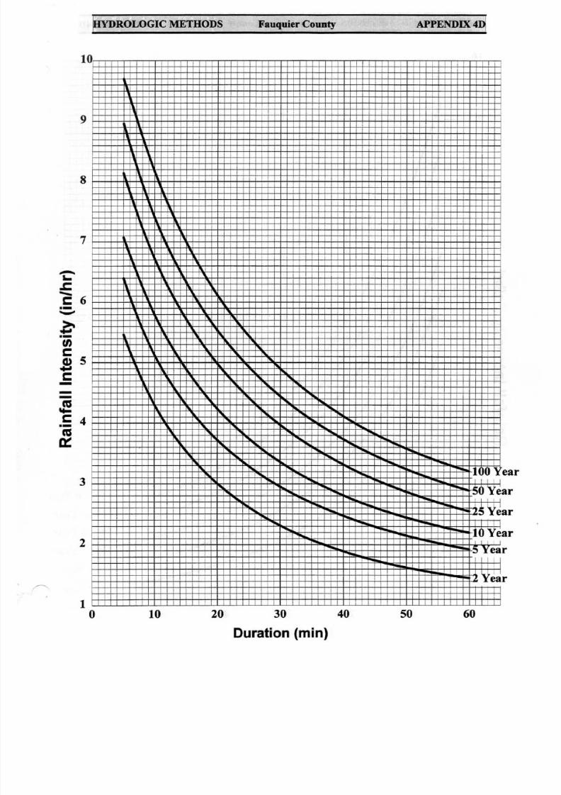
7/30/2019 Virginia Stormwater Managment Handbook Volume_II.pdf
http://slidepdf.com/reader/full/virginia-stormwater-managment-handbook-volumeiipdf 104/354
7/30/2019 Virginia Stormwater Managment Handbook Volume_II.pdf
http://slidepdf.com/reader/full/virginia-stormwater-managment-handbook-volumeiipdf 105/354

7/30/2019 Virginia Stormwater Managment Handbook Volume_II.pdf
http://slidepdf.com/reader/full/virginia-stormwater-managment-handbook-volumeiipdf 106/354
7/30/2019 Virginia Stormwater Managment Handbook Volume_II.pdf
http://slidepdf.com/reader/full/virginia-stormwater-managment-handbook-volumeiipdf 107/354

7/30/2019 Virginia Stormwater Managment Handbook Volume_II.pdf
http://slidepdf.com/reader/full/virginia-stormwater-managment-handbook-volumeiipdf 108/354

7/30/2019 Virginia Stormwater Managment Handbook Volume_II.pdf
http://slidepdf.com/reader/full/virginia-stormwater-managment-handbook-volumeiipdf 109/354

7/30/2019 Virginia Stormwater Managment Handbook Volume_II.pdf
http://slidepdf.com/reader/full/virginia-stormwater-managment-handbook-volumeiipdf 110/354

7/30/2019 Virginia Stormwater Managment Handbook Volume_II.pdf
http://slidepdf.com/reader/full/virginia-stormwater-managment-handbook-volumeiipdf 111/354
7/30/2019 Virginia Stormwater Managment Handbook Volume_II.pdf
http://slidepdf.com/reader/full/virginia-stormwater-managment-handbook-volumeiipdf 112/354

7/30/2019 Virginia Stormwater Managment Handbook Volume_II.pdf
http://slidepdf.com/reader/full/virginia-stormwater-managment-handbook-volumeiipdf 113/354

7/30/2019 Virginia Stormwater Managment Handbook Volume_II.pdf
http://slidepdf.com/reader/full/virginia-stormwater-managment-handbook-volumeiipdf 114/354

7/30/2019 Virginia Stormwater Managment Handbook Volume_II.pdf
http://slidepdf.com/reader/full/virginia-stormwater-managment-handbook-volumeiipdf 115/354

7/30/2019 Virginia Stormwater Managment Handbook Volume_II.pdf
http://slidepdf.com/reader/full/virginia-stormwater-managment-handbook-volumeiipdf 116/354

7/30/2019 Virginia Stormwater Managment Handbook Volume_II.pdf
http://slidepdf.com/reader/full/virginia-stormwater-managment-handbook-volumeiipdf 117/354
CHAPTER 5
ENGINEERING
CALCULATIONS

7/30/2019 Virginia Stormwater Managment Handbook Volume_II.pdf
http://slidepdf.com/reader/full/virginia-stormwater-managment-handbook-volumeiipdf 118/354
ENGINEERING CALCULATIONS CHAPTER 5

7/30/2019 Virginia Stormwater Managment Handbook Volume_II.pdf
http://slidepdf.com/reader/full/virginia-stormwater-managment-handbook-volumeiipdf 119/354
ENGINEERING CALCULATIONS CHAPTER 5
5-i
TABLE OF CONTENTS
# SECTIONS PAGE
5-1 INTRODUCTION . . . . . . . . . . . . . . . . . . . . . . . . . . . . . . . . . . . . . . . . . . . . . . . . . . 5-1
5-2 GENERAL INFORMATION: DETENTION, EXTENDED-DETENTION
AND RETENTION BASIN DESIGN CALCULATIONS . . . . . . . . . . . . . . . 5-1
5-3 ALLOWABLE RELEASE RATES . . . . . . . . . . . . . . . . . . . . . . . . . . . . . . . . . . . . 5-2
5-4 STORAGE VOLUME REQUIREMENT ESTIMATES . . . . . . . . . . . . . . . . . . . . 5-3
5-4.1 Graphical Hydrograph Analysis - SCS Methods . . . . . . . . . . . . . . . . . . 5-4
5-4.2 TR-55: Storage Volume for Detention Basins (Shortcut Method) . . . . 5-8
5-4.3 Graphical Hydrograph Analysis, Modified Rational Method -Critical Storm Duration . . . . . . . . . . . . . . . . . . . . . . . . . . . . . . 5-12
5-4.4 Modified Rational Method, Critical Storm Duration - Direct Solution . 5-18
5-5 STAGE-STORAGE CURVE . . . . . . . . . . . . . . . . . . . . . . . . . . . . . . . . . . . . . . . . . 5-27
5-5.1 Storage Volume Calculations . . . . . . . . . . . . . . . . . . . . . . . . . . . . . . . . . 5-27
5-6 WATER QUALITY AND CHANNEL EROSION CONTROL
VOLUME CALCULATIONS . . . . . . . . . . . . . . . . . . . . . . . . . . . . . . . . . . . . 5-30
5-6.1 Retention Basins - Water Quality Volume . . . . . . . . . . . . . . . . . . . . . . . 5-31
5-6.2 Extended-Detention Basins - Water Quality Volume and Orifice Design 5-33
5-6.3 Extended-Detention Basins - Channel Erosion Control Volume andOrifice Design . . . . . . . . . . . . . . . . . . . . . . . . . . . . . . . . . . . . . 5-38
5-7 MULTI-STAGE RISER DESIGN . . . . . . . . . . . . . . . . . . . . . . . . . . . . . . . . . . . . . 5-41
5-8 EMERGENCY SPILLWAY DESIGN . . . . . . . . . . . . . . . . . . . . . . . . . . . . . . . . . . 5-71
5-9 HYDROGRAPH ROUTING . . . . . . . . . . . . . . . . . . . . . . . . . . . . . . . . . . . . . . . . . 5-82
5-10 WATER QUALITY CALCULATION PROCEDURES . . . . . . . . . . . . . . . . . . . . 5-94
5-10.1 Performance-Based Water Quality Criteria . . . . . . . . . . . . . . . . . . . . . . 5-94
5-10.2 Performance-Based Water Quality Calculation Procedures . . . . . . . . . . 5-97

7/30/2019 Virginia Stormwater Managment Handbook Volume_II.pdf
http://slidepdf.com/reader/full/virginia-stormwater-managment-handbook-volumeiipdf 120/354
ENGINEERING CALCULATIONS CHAPTER 5
5-ii
LIST OF ILLUSTRATIONS
# FIGURES PAGE
5 - 1 SCS Runoff Hydrograph, Example 1, 2-Year Post-Developed . . . . . . . . . . . . 5-55 - 2 SCS Runoff Hydrograph, Example 1, 10-Year Post-Developed . . . . . . . . . . . 5-7
5 - 3 Typical Outlet Rating Curves for Orifice and Weir Outlet Devices . . . . . . . . 5-8
5 - 4 Approximate Detention Basin Routing for Rainfall Types I, IA, II, and III . . 5-11
5 - 5 Modified Rational Method Hydrographs . . . . . . . . . . . . . . . . . . . . . . . . . . . . . 5-13
5 - 6 Modified Rational Method Runoff Hydrograph, Example 1,
2-Year Post-Developed Condition . . . . . . . . . . . . . . . . . . . . . . . . . . . . . 5-16
5 - 7 Modified Rational Method Runoff Hydrograph, Example 1,
10-Year Post-Developed Condition . . . . . . . . . . . . . . . . . . . . . . . . . . . . 5-17
5 - 8 Trapezoidal Hydrograph Storage Volume Estimate . . . . . . . . . . . . . . . . . . . . 5-19
5 - 9 Storage Volume vs. Time Curve . . . . . . . . . . . . . . . . . . . . . . . . . . . . . . . . . . . 5-22
5 - 10 Stage-Storage Computation Worksheet, Example 1 . . . . . . . . . . . . . . . . . . . . 5-295 - 11 Stage vs. Storage Curve, Example 1 . . . . . . . . . . . . . . . . . . . . . . . . . . . . . . . . 5-31
5 - 12 Weir and Orifice Flow . . . . . . . . . . . . . . . . . . . . . . . . . . . . . . . . . . . . . . . . . . . 5-45
5 - 13 Stage-Storage-Discharge Worksheet, Example 1 . . . . . . . . . . . . . . . . . . . . . . 5-54
5 - 14 Typical Hydraulic Head Values - Multi-Stage Riser . . . . . . . . . . . . . . . . . . . 5-55
5 - 15 a-d Riser Flow Diagrams . . . . . . . . . . . . . . . . . . . . . . . . . . . . . . . . . . . . . . . . . . . . 5-56
5 - 16 Headwater Depth for Concrete Pipe Culverts with Inlet Control . . . . . . . . . . 5-57
5 - 17 Headwater Depth Entrance Conditions . . . . . . . . . . . . . . . . . . . . . . . . . . . . . . 5-58
5 - 18 Hydraulic Head Values - Barrel Flow . . . . . . . . . . . . . . . . . . . . . . . . . . . . . . . 5-58
5 - 19 Outlet Protection Detail . . . . . . . . . . . . . . . . . . . . . . . . . . . . . . . . . . . . . . . . . . 5-63
5 - 20 Minimum Tailwater Condition . . . . . . . . . . . . . . . . . . . . . . . . . . . . . . . . . . . . 5-64
5 - 21 Maximum Tailwater Condition . . . . . . . . . . . . . . . . . . . . . . . . . . . . . . . . . . . . 5-655 - 22 Phreatic Line Graphical Determination . . . . . . . . . . . . . . . . . . . . . . . . . . . . . . 5-69
5 - 23 Vegetated Emergency Spillways: Typical Plan and Section . . . . . . . . . . . . . . 5-81
5 - 24 Stage vs. Discharge Curve, Example 1 . . . . . . . . . . . . . . . . . . . . . . . . . . . . . . 5-87
5 - 25 Storage Indication Hydrograph Routing (2S/ ∆t + O) vs. O Worksheet . . . . . 5-88
5 - 26 Storage Indication Hydrograph Routing (2S/ ∆t + O) vs. O Worksheet,
Example 1, Curve & Table . . . . . . . . . . . . . . . . . . . . . . . . . . . . . . . . . . . 5-89
5 - 27 Storage Indication Hydrograph Routing Worksheet . . . . . . . . . . . . . . . . . . . . 5-90
5 - 28 Storage Indication Hydrograph Routing Worksheet, Example 1 . . . . . . . . . . 5-92
5 - 29 Inflow and Discharge Hydrographs, Example 1 . . . . . . . . . . . . . . . . . . . . . . . 5-93

7/30/2019 Virginia Stormwater Managment Handbook Volume_II.pdf
http://slidepdf.com/reader/full/virginia-stormwater-managment-handbook-volumeiipdf 121/354
ENGINEERING CALCULATIONS CHAPTER 5
5-iii
LIST OF ILLUSTRATIONS (con’t.)
# TABLES PAGE
5 - 1 Hydrologic Summary, Example 1, SCS Methods . . . . . . . . . . . . . . . . . . . . . . 5-35 - 2 Storage Volume Requirements, Example 1 . . . . . . . . . . . . . . . . . . . . . . . . . . . 5-11
5 - 3 Hydrologic Summary, Example 1, Rational Method . . . . . . . . . . . . . . . . . . . . 5-14
5 - 4 Storage Volume Requirements, Example 1 . . . . . . . . . . . . . . . . . . . . . . . . . . . 5-15
5 - 5 Rainfall Constants for Virginia . . . . . . . . . . . . . . . . . . . . . . . . . . . . . . . . . . . . 5-20
5 - 6 Summary of Results: Storage Volume Requirement Estimates, Example 1 . 5-27
5 - 7 Stage-Discharge Table: Water Quality Orifice Design . . . . . . . . . . . . . . . . . 5-37
5 - 8 Weir Flow Coefficients . . . . . . . . . . . . . . . . . . . . . . . . . . . . . . . . . . . . . . . . . . 5-47
5 - 9 Pipe Entrance Loss Coefficients, K e . . . . . . . . . . . . . . . . . . . . . . . . . . . . . . . . 5-59
5 - 10 Head Loss Coefficients, K p, for Circular and Square Conduits Flowing Full . 5-60
5 - 11 Graded Riprap Design Values . . . . . . . . . . . . . . . . . . . . . . . . . . . . . . . . . . . . . 5-62
5 - 12 Design Data for Earth Spillways . . . . . . . . . . . . . . . . . . . . . . . . . . . . . . . . . . . 5-775 - 13 H p and Slope Range for Discharge, Velocity, and Crest Length -
a. Retardance A . . . . . . . . . . . . . . . . . . . . . . . . . . . . . . . . . . . . . . . . . . . . 5-78
b. Retardance B . . . . . . . . . . . . . . . . . . . . . . . . . . . . . . . . . . . . . . . . . . . . 5-79
c. Retardance C . . . . . . . . . . . . . . . . . . . . . . . . . . . . . . . . . . . . . . . . . . . . 5-79
d. Retardance D . . . . . . . . . . . . . . . . . . . . . . . . . . . . . . . . . . . . . . . . . . . . 5-80
5 - 14 Water Quality BMP Pollutant Removal Efficiencies . . . . . . . . . . . . . . . . . . 5-106
5 - 15 Simple Method General Pollutant Load Equation Solved for Incremental
Impervious Cover Values . . . . . . . . . . . . . . . . . . . . . . . . . . . . . . . . . . . . . . . 5-107
# EQUATIONS PAGE
5 - 1 Trapezoidal Hydrograph Storage Volume Equation . . . . . . . . . . . . . . . . . . . . 5-18
5 - 2 Modified Rational Method Intensity, I , Equation . . . . . . . . . . . . . . . . . . . . . . 5-19
5 - 3 Rearranged Rational Equation . . . . . . . . . . . . . . . . . . . . . . . . . . . . . . . . . . . . . 5-20
5 - 4 Substitute Eq. 5-3 into Eq. 5-1 . . . . . . . . . . . . . . . . . . . . . . . . . . . . . . . . . . . . . 5-21
5 - 5 Critical Storm Duration, T d . . . . . . . . . . . . . . . . . . . . . . . . . . . . . . . . . . . . . . . 5-21
5 - 6 Orifice Equation . . . . . . . . . . . . . . . . . . . . . . . . . . . . . . . . . . . . . . . . . . . . . . . . 5-35
5 - 7 Rearranged Orifice Equation . . . . . . . . . . . . . . . . . . . . . . . . . . . . . . . . . . . . . . 5-35
5 - 8 Weir Equation . . . . . . . . . . . . . . . . . . . . . . . . . . . . . . . . . . . . . . . . . . . . . . . . . 5-44
5 - 9 Rearranged Weir Equation . . . . . . . . . . . . . . . . . . . . . . . . . . . . . . . . . . . . . . . . 5-46
5 - 10 Pipe Flow Control Equation . . . . . . . . . . . . . . . . . . . . . . . . . . . . . . . . . . . . . . 5-515 - 11 Barrel Length in Saturated Zone . . . . . . . . . . . . . . . . . . . . . . . . . . . . . . . . . . . 5-68
5 - 12 Continuity Equation . . . . . . . . . . . . . . . . . . . . . . . . . . . . . . . . . . . . . . . . . . . . . 5-85
5 - 13 Rearranged Continuity Equation . . . . . . . . . . . . . . . . . . . . . . . . . . . . . . . . . . . 5-85
5 - 14 Simple Method Pollutant Load . . . . . . . . . . . . . . . . . . . . . . . . . . . . . . . . . . . . 5-95
7/30/2019 Virginia Stormwater Managment Handbook Volume_II.pdf
http://slidepdf.com/reader/full/virginia-stormwater-managment-handbook-volumeiipdf 122/354
ENGINEERING CALCULATIONS CHAPTER 5
5-iv
LIST OF ILLUSTRATIONS (con’t.)
# EQUATIONS PAGE
5 - 15 Simple Method Pollutant Load Simplified . . . . . . . . . . . . . . . . . . . . . . . . . . . 5-95
5 - 16 Pollutant Load Based on Average Land Cover Conditions . . . . . . . . . . . . . . 5-100
5 - 17 Pollutant Load Based on Existing Site Conditions . . . . . . . . . . . . . . . . . . . . 5-101
5 - 18 Pollutant Load to Existing BMP . . . . . . . . . . . . . . . . . . . . . . . . . . . . . . . . . . 5-102
5 - 19 Pollutant Load Removed by Existing BMP . . . . . . . . . . . . . . . . . . . . . . . . . . 5-102
5 - 20 Pollutant Load Based on Existing BMP Removal Efficiency . . . . . . . . . . . . 5-102
5 - 21 Pollutant Load Based on Post-Development Site Conditions . . . . . . . . . . . . 5-103
5 - 22 Required Pollutant Removal Efficiency . . . . . . . . . . . . . . . . . . . . . . . . . . . . 5-104
5 - 23 Pollutant Load Entering Proposed BMP . . . . . . . . . . . . . . . . . . . . . . . . . . . . 5-104
5 - 24 Pollutant Load Removed by Proposed BMP . . . . . . . . . . . . . . . . . . . . . . . . . 5-105
5 - 25 Total Pollutant Load Removed by Existing and Proposed BMPs . . . . . . . . . 5-105

7/30/2019 Virginia Stormwater Managment Handbook Volume_II.pdf
http://slidepdf.com/reader/full/virginia-stormwater-managment-handbook-volumeiipdf 123/354
ENGINEERING CALCULATIONS CHAPTER 5
5-1
ENGINEERING CALCULATIONS
5-1 INTRODUCTION
This section provides guidelines for performing various engineering calculations associated with the
design of stormwater management facilities such as extended-detention and retention basins and
multi-stage outlet structures. The prerequisite information for using these calculations is the
determination of the hydrologic characteristics of the contributing watershed in the form of the peak
discharge (in cfs), or a runoff hydrograph, depending on the hydrologic and hydraulic routing
methods used. (Refer to Section 4-4 in Chapter 4 for hydrologic methods.)
5-2 GENERAL INFORMATION: DETENTION, EXTENDED-DETENTION AND
RETENTION BASIN DESIGN CALCULATIONS
Based on Virginia’s Stormwater Management Regulations, a stormwater management basin may be designed to control water quantity (for flood control and channel erosion control) and to enhance
(or treat) water quality. The type of basin selected (extended-detention, retention, infiltration, etc.)
and the relationship between its design components (design inflow, storage volume and outflow) will
dictate the size of the basin and serve as the basis for its hydraulic design. Some design component
parameters such as design storm return frequency, allowable discharge rates, etc., may be specified
by the local regulatory authority, based upon the specific needs of certain watersheds or stream
channels within that locality. Occasionally, as in stream channel erosion control, it may be up to the
engineer to document and analyze the specific needs of the downstream channel and establish the
design parameters.
The design inflow is either the peak flow or the runoff hydrograph from the developed watershed.This inflow becomes the input data for the basin sizing calculations, often called routings. Various
routing methods are available. Note that the format of the hydrologic input data will usually be
dictated by whatever routing method is chosen. (The methods discussed in this handbook require
the use of a peak discharge or an actual runoff hydrograph.) Generally, larger and more complex
projects will require a detailed analysis, which includes a runoff hydrograph. Preliminary studies
and small projects may be designed using simpler, shortcut techniques that only require a peak
discharge. For all projects, the designer must document the hydrologic conditions to support the
inflow portion of the hydraulic relationship.
Achieving adequate storage volume within a basin can usually be accomplished by manipulation
of the site grades and strategic placement of the permanent features such as buildings and parkinglots. Sometimes, the location of a stormwater facility will be dictated by the site topography and
available outfall location. (Refer to Chapter 3 for basin planning considerations and design
criteria.) Storage volume calculations will be discussed in detail later in this chapter.

7/30/2019 Virginia Stormwater Managment Handbook Volume_II.pdf
http://slidepdf.com/reader/full/virginia-stormwater-managment-handbook-volumeiipdf 124/354
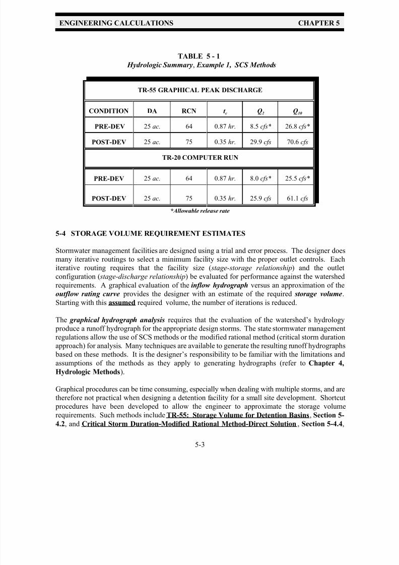
7/30/2019 Virginia Stormwater Managment Handbook Volume_II.pdf
http://slidepdf.com/reader/full/virginia-stormwater-managment-handbook-volumeiipdf 125/354
ENGINEERING CALCULATIONS CHAPTER 5
5-3
TABLE 5 - 1
Hydrologic Summary, Example 1, SCS Methods
TR-55 GRAPHICAL PEAK DISCHARGE
CONDITION DA RCN t c Q2 Q10
PRE-DEV 25 ac. 64 0.87 hr. 8.5 cfs* 26.8 cfs*
POST-DEV 25 ac. 75 0.35 hr. 29.9 cfs 70.6 cfs
TR-20 COMPUTER RUN
PRE-DEV 25 ac. 64 0.87 hr. 8.0 cfs* 25.5 cfs*
POST-DEV 25 ac. 75 0.35 hr. 25.9 cfs 61.1 cfs
*Allowable release rate
5-4 STORAGE VOLUME REQUIREMENT ESTIMATES
Stormwater management facilities are designed using a trial and error process. The designer does
many iterative routings to select a minimum facility size with the proper outlet controls. Each
iterative routing requires that the facility size ( stage-storage relationship) and the outlet
configuration ( stage-discharge relationship) be evaluated for performance against the watershed
requirements. A graphical evaluation of the inflow hydrograph versus an approximation of theoutflow rating curve provides the designer with an estimate of the required storage volume.
Starting with this assumed required volume, the number of iterations is reduced.
The graphical hydrograph analysis requires that the evaluation of the watershed’s hydrology
produce a runoff hydrograph for the appropriate design storms. The state stormwater management
regulations allow the use of SCS methods or the modified rational method (critical storm duration
approach) for analysis. Many techniques are available to generate the resulting runoff hydrographs
based on these methods. It is the designer’s responsibility to be familiar with the limitations and
assumptions of the methods as they apply to generating hydrographs (refer to Chapter 4,
Hydrologic Methods).
Graphical procedures can be time consuming, especially when dealing with multiple storms, and are
therefore not practical when designing a detention facility for a small site development. Shortcut
procedures have been developed to allow the engineer to approximate the storage volume
requirements. Such methods include TR-55: Storage Volume for Detention Basins, Section 5-
4.2, and Critical Storm Duration-Modified Rational Method-Direct Solution, Section 5-4.4,

7/30/2019 Virginia Stormwater Managment Handbook Volume_II.pdf
http://slidepdf.com/reader/full/virginia-stormwater-managment-handbook-volumeiipdf 126/354
ENGINEERING CALCULATIONS CHAPTER 5
5-4
Procedure
which can be used as planning tools. Final design should be refined using a more accurate
hydrograph routing procedure. Sometimes, these shortcut methods may be used for final design, but
they must be used with caution since they only approximate the required storage volume (refer to
the assumptions and limitations for each method).
It should be noted that the TR-55 tabular hydrograph method does not produce a full hydrograph.
The tabular method generates only the portion of the hydrograph that contains the peak discharge
and some of the time steps just before and just after the peak. The missing values must be
extrapolated, thus potentially reducing the accuracy of the hydrograph analysis. It is recommended
that if SCS methods are to be used, a full hydrograph be generated using one of the available
computer programs. The accuracy of the analysis can only be as accurate as the hydrograph used.
5-4.1 Graphical Hydrograph Analysis - SCS Methods
The following procedure represents a graphical hydrograph analysis that results in the approximation
of the required storage volume for a proposed stormwater management basin. Example 1 is presented here to illustrate this technique. See Table 5-1 for a summary of the hydrology. The TR-
20 computer-generated inflow hydrograph is used for this example. The allowable discharge from
the proposed basin has been established by ordinance (based on pre-developed watershed discharge).
Information Needed:
The pre- and post-developed hydrology, which includes the pre-developed peak rate of runoff
(allowable release rate) and the post-developed runoff hydrograph (inflow hydrograph) is required
for hydrograph analysis (see Table 5-1).
(Refer to Figure 5-1 for the 2-year developed inflow hydrograph and Figure 5-2 for the 10-year
developed inflow hydrograph):
1. Commencing with the plot of the 2-year developed inflow hydrograph (Discharge vs. Time),
the 2-year allowable release rate, Q2 = 8 cfs, is plotted as a horizontal line starting at time t =
0 and continuing to the point where it intersects the falling limb of the hydrograph.
2. A diagonal line is then drawn from the beginning of the inflow hydrograph to the intersection
point described above. This line represents the hypothetical rating curve of the control
structure and approximates the rising limb of the outflow hydrograph for the 2-year storm.

7/30/2019 Virginia Stormwater Managment Handbook Volume_II.pdf
http://slidepdf.com/reader/full/virginia-stormwater-managment-handbook-volumeiipdf 127/354
ENGINEERING CALCULATIONS CHAPTER 5
5-5
FIGURE 5 - 1
SCS Runoff Hydrograph, Example 1, 2-Year Post-Developed
3. The storage volume is then approximated by calculating the area under the inflow hydrograph,
less the area under the rising limb of the outflow hydrograph. This is shown as the shaded area
in Figure 5-1. The storage volume required for the 2-year storm, S 2 , can be approximated by
measuring the shaded area with a planimeter.
The vertical scale of a hydrograph is in cubic feet per second (cfs) and the horizontal scale is in
hours (hrs). Therefore, the area, as measured in square inches (in2 ), is multiplied by scale conversion
factors of cfs per inch, hours per inch, and 3600 seconds per hour, to yield an area in cubic feet ( ft 3).
The conversion is as follows:
S 2 = (0.398 in2 )(10 cfs/in.)(2.5 hrs./in.)(3,600 sec./hr.)
= 35,820 ft 3
= 0.82 ac.ft.
7/30/2019 Virginia Stormwater Managment Handbook Volume_II.pdf
http://slidepdf.com/reader/full/virginia-stormwater-managment-handbook-volumeiipdf 128/354
ENGINEERING CALCULATIONS CHAPTER 5
5-6
4. On a plot of the 10-year inflow hydrograph, the 10-year allowable release rate, Q10 , is
plotted as a horizontal line extending from time zero to the point where it intersects the
falling limb of the hydrograph.
5. By trial and error, the time t 2 , at which the S 2 volume occurs while maintaining the 2-year release, is determined by planimeter. This is represented by the shaded area to the left of t 2on Figure 5-2. From the intersection point of t 2 and the 2-year allowable release rate, Q2 ,
a line is drawn to connect to the intersection point of the 10-year allowable release rate and
the falling limb of the hydrograph. This intersection point is t 10 , and the connecting line is
a straight line approximation of the outlet rating curve.
6. The area under the inflow hydrograph from time t 2 to time t 10 , less the area under the rising
limb of the hypothetical rating curve, represents the additional volume (shaded area to the
right of t 2 on Figure 5-2) needed to meet the 10-year storm storage requirements.
7. The total storage volume, S 10 , required, can be computed by adding this additional storagevolume to S 2 . This is represented by the total shaded area under the hydrograph.
S 10 = (0.89 in2 )(10 cfs/in.)(2.5 hrs./in.)(3,600 sec./hr.)
= 80,100 ft 3
= 1.84 ac.ft.
These steps may be repeated if storage of the 100-year storm, or any other design frequency storm,
is required by ordinance or downstream conditions.
In summary, the total volume of storage required is the area under the runoff hydrograph
curve and above the basin outflow curve. It should be noted that the outflow rating curve is
approximated as a straight line. The actual shape of the outflow rating curve will depend on the type
of outlet device used. Figure 5-3 shows the typical shapes of outlet rating curves for orifice and
weir outlet structures. The straight line approximation is reasonable for an orifice outlet structure.
However, this approximation will likely underestimate the storage volume required when a weir
outlet structure is used. Depending on the complexity of the design and the need for an exact
engineered solution, the use of a more rigorous sizing technique, such as a storage indication
routing, may be necessary.
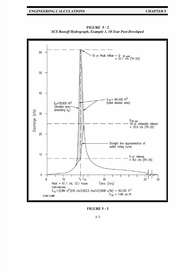
7/30/2019 Virginia Stormwater Managment Handbook Volume_II.pdf
http://slidepdf.com/reader/full/virginia-stormwater-managment-handbook-volumeiipdf 129/354
ENGINEERING CALCULATIONS CHAPTER 5
5-7
FIGURE 5 - 2
SCS Runoff Hydrograph, Example 1, 10-Year Post-Developed
FIGURE 5 - 3

7/30/2019 Virginia Stormwater Managment Handbook Volume_II.pdf
http://slidepdf.com/reader/full/virginia-stormwater-managment-handbook-volumeiipdf 130/354
ENGINEERING CALCULATIONS CHAPTER 5
5-8
Typical Outlet Rating Curves for Orifice and Weir Outlet Devices
5-4.2 TR-55: Storage Volume for Detention Basins (Shortcut Method)
The TR-55 Storage Volume for Detention Basins, or TR-55 shortcut procedure, provides similar
results to the graphical analysis described in Section 5-4.1. This method is based on average storage
and routing effects for many structures. TR-55 can be used for single-stage or multi-stage outflowdevices. The only constraints are that 1) each stage requires a design storm and a computation of
the storage required for it , and 2) the discharge of the upper stage(s) includes the discharge of the
lower stage(s). Refer to TR-55 for more detailed discussions and limitations.
Information Needed:
To calculate the required storage volume using TR-55, the pre- and post-developed hydrology per
SCS methods is needed (refer to Chapter 4). This includes the watershed’s pre-developed peak
rate of discharge, or allowable release rate, Qo , the watershed’s post-developed peak rate of
discharge, or inflow, Qi , for the appropriate design storms, and the watershed’s post-developed
runoff , Q, in inches. (Note that this method does not require a hydrograph.)
Once the above parameters are known, the TR-55 Manual can be used to approximate the storage
volume required for each design storm. The following procedure summarizes the TR-55 shortcut
method using the 25-acre watershed presented in Example 1.
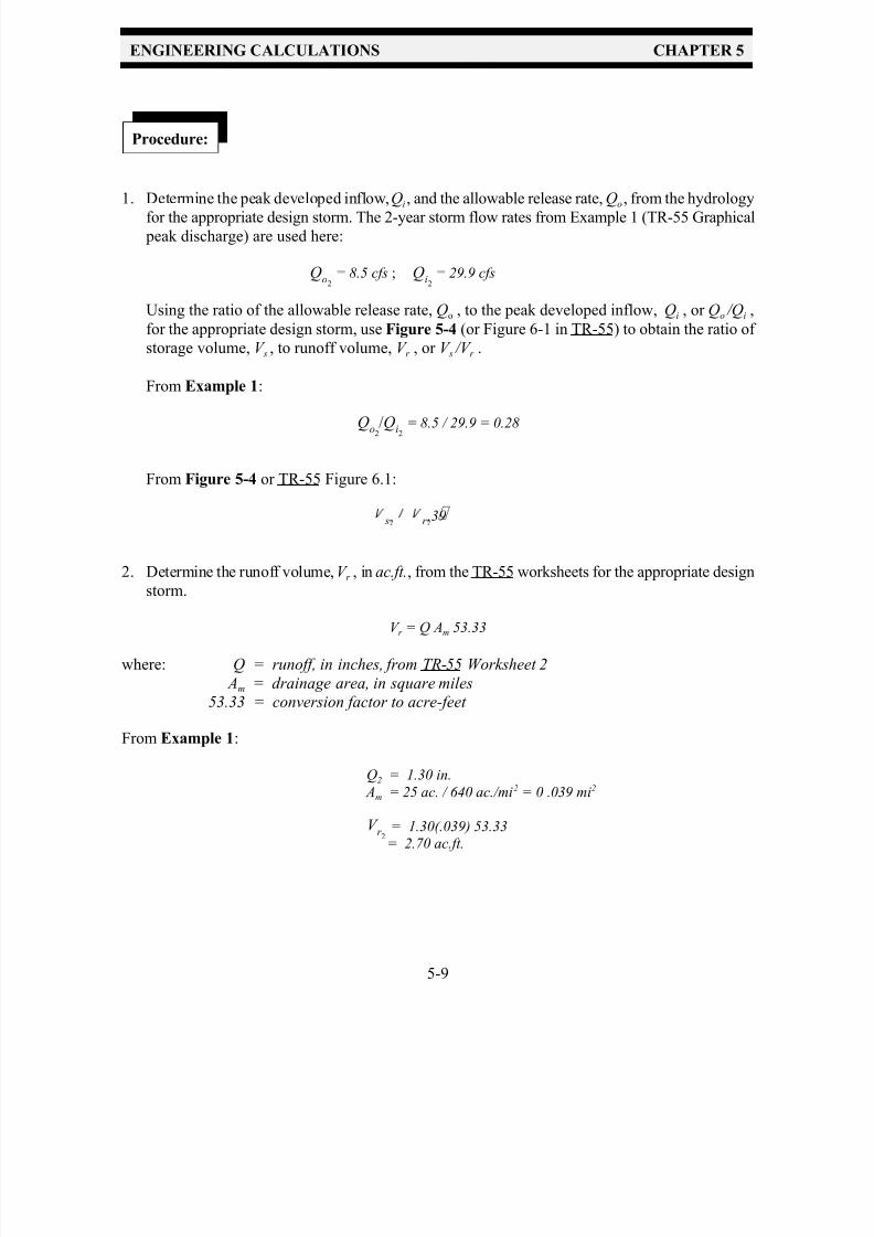
7/30/2019 Virginia Stormwater Managment Handbook Volume_II.pdf
http://slidepdf.com/reader/full/virginia-stormwater-managment-handbook-volumeiipdf 131/354
ENGINEERING CALCULATIONS CHAPTER 5
5-9
Procedure:
s r '
V r 2
1. Determine the peak developed inflow, Qi , and the allowable release rate, Qo , from the hydrologyfor the appropriate design storm. The 2-year storm flow rates from Example 1 (TR-55 Graphical
peak discharge) are used here:
= 8.5 cfs ; = 29.9 cfsQo2
Qi2
Using the ratio of the allowable release rate, Qo , to the peak developed inflow, Qi , or Qo /Qi ,
for the appropriate design storm, use Figure 5-4 (or Figure 6-1 in TR-55) to obtain the ratio of
storage volume, V s , to runoff volume, V r , or V s /V r .
From Example 1:
= 8.5 / 29.9 = 0.28Qo2
/Qi2
From Figure 5-4 or TR-55 Figure 6.1:
.39
2. Determine the runoff volume, V r , in ac.ft., from the TR-55 worksheets for the appropriate design
storm.
V r = Q Am 53.33
where: Q = runoff, in inches, from TR-55 Worksheet 2
Am = drainage area, in square miles
53.33 = conversion factor to acre-feet
From Example 1:
Q2 = 1.30 in.
Am = 25 ac. / 640 ac./mi2 = 0 .039 mi2
= 1.30(.039) 53.33= 2.70 ac.ft.

7/30/2019 Virginia Stormwater Managment Handbook Volume_II.pdf
http://slidepdf.com/reader/full/virginia-stormwater-managment-handbook-volumeiipdf 132/354
ENGINEERING CALCULATIONS CHAPTER 5
5-10
V s
V r
V r ' V s
3. Multiply the V s /V r ratio from Step 1 by the runoff volume, V r , from Step 2, to determine the
volume of storage required, V s , in acre-feet.
From Example 1:
(.39)(2.70 ac.ft.) = 1.05 ac.ft.
4. Repeat these steps for each additional design storm as required to determine the approximate
storage requirements. The 10-year storm storage requirements from Example 1 are presented
here:
a. Qo = 26.8 cfsQi = 70.6 cfs
Qo /Qi = 26.8/70.6 = 0.38; From Figure 5-4 or TR-55 Figure 6-1: V s /V r = .33
b. V r = QAm 53.33 = 2.85 in.(.039 sq.mi.)(53.33) = 5.93 ac.ft.
c. V s = (V s /V r )V r = (.33) 5.93 ac.ft. = 1.96 ac.ft.
This volume represents the total storage required for the 2-year storm and the 10-year storm.
5. NOTE: The volume from #4 above may need to be increased if additional storage is required
for water quality purposes or channel erosion control. Refer to Section 5-6 or Section 5-10,
respectively.
The design procedure presented above should be used with TR-55 Worksheet 6a, as shown in
Example 1 of Chapter 6. The worksheet includes an area to plot the stage-storage curve, from
which actual elevations corresponding to the required storage volumes can be derived. Table 5-2
provides a summary of the required storage volumes using the graphical SCS hydrograph analysis
and the TR-55 shortcut method.

7/30/2019 Virginia Stormwater Managment Handbook Volume_II.pdf
http://slidepdf.com/reader/full/virginia-stormwater-managment-handbook-volumeiipdf 133/354
ENGINEERING CALCULATIONS CHAPTER 5
5-11
TABLE 5 - 2
Storage Volume Requirements, Example 1
Method 2- yr . StorageRequired 10- yr . StorageRequired
Graphical Hydrograph Analysis 0.82 ac.ft. 1.84 ac.ft.
TR-55 Shortcut Method 1.05 ac.ft. 1.96 ac.ft.
FIGURE 5 - 4
Approximate Detention Basin Routing for Rainfall Types I, IA, II and III
Source: SCS TR-55 Urban Hydrology for Small Watersheds: Figure 6-1

7/30/2019 Virginia Stormwater Managment Handbook Volume_II.pdf
http://slidepdf.com/reader/full/virginia-stormwater-managment-handbook-volumeiipdf 134/354
ENGINEERING CALCULATIONS CHAPTER 5
5-12
5-4.3 Graphical Hydrograph Analysis, Modified Rational Method - Critical Storm Duration
The Modified Rational Method uses the critical storm duration to calculate the maximum storage
volume for a detention facility. This critical storm duration is the storm duration that generates the
greatest volume of runoff and, therefore, requires the most storage. In contrast, the Rational Method produces a triangular runoff hydrograph that gives the peak inflow at time = t c and falls to zero flow
at time = 2.5t c . In theory, this hydrograph represents a storm whose duration equals the time of
concentration, t c , resulting in the greatest peak discharge for the given return frequency storm. The
volume of runoff, however, is of greater consequence in sizing a detention facility. A storm whose
duration is longer than the t c may not produce as large a peak rate of runoff, but it may generate a
greater volume of runoff. By using the Modified Rational Method, the designer can evaluate several
different storm durations to verify which one requires the greatest volume of storage with respect
to the allowable release rate. It is this maximum storage volume that the basin must be designed to
detain.
The first step in determining the critical storm duration is to use the post-developed time of concentration, t c , to generate a post-developed runoff hydrograph. Rainfall intensity averaging
periods, T d , representing time periods incrementally longer than the t c , are then used to generate a
“family” of runoff hydrographs for the same drainage area. These hydrographs will be trapezoidal
with the peak discharges, Qi , based upon the intensity, I , of the averaging period, T d . Figure 5-5
shows the construction of a typical triangular and trapezoidal hydrograph using the modified rational
method, and a family of trapezoidal hydrographs representing storms of different durations.
Note that the duration of the receding limb of the trapezoidal hydrograph, in Figure 5-5, is set to
equal 1.5 times the time of concentration, t c . Also, the total hydrograph duration is 2.5t c versus 2t cas discussed in Chapter 4. This longer duration is considered more representative of actual storm
and runoff dynamics. It is also more analogous to the SCS unit hydrograph where the receding limbextends longer than the rising limb.
The Modified Rational Method assumes that the rainfall intensity averaging period is equal to the
actual storm duration. This means that the rainfall and runoff that occur before and after the rainfall
averaging period are not accounted for. Therefore, the Modified Rational Method may
underestimate the required storage volume for any given storm event.
The rainfall intensity averaging periods are chosen arbitrarily. However, the designer should select
periods for which the corresponding intensity-duration-frequency (I-D-F) curves are available, i.e.,
10 min., 20 min., 30 min., etc. The shortest period selected should be the time of concentration, t c .
A straight line starting at Q = 0 and t = 0 and intercepting the inflow hydrograph on the recedinglimb at the allowable release rate, Qo , represents the outflow rating curve. The time averaging
period hydrograph that represents the greatest storage volume required is the one with the largest
area between the inflow hydrograph and outflow rating curve. This determination is made by a
graphical analysis of the hydrographs.
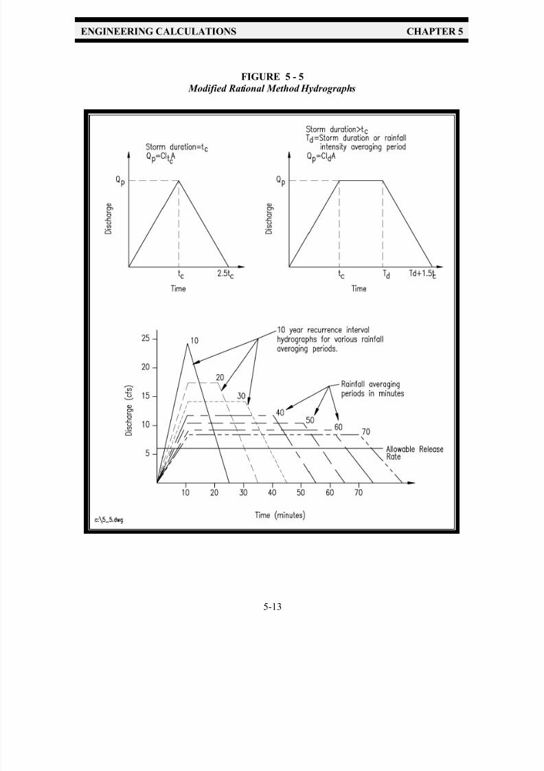
7/30/2019 Virginia Stormwater Managment Handbook Volume_II.pdf
http://slidepdf.com/reader/full/virginia-stormwater-managment-handbook-volumeiipdf 135/354
ENGINEERING CALCULATIONS CHAPTER 5
5-13
FIGURE 5 - 5
Modified Rational Method Hydrographs
7/30/2019 Virginia Stormwater Managment Handbook Volume_II.pdf
http://slidepdf.com/reader/full/virginia-stormwater-managment-handbook-volumeiipdf 136/354
ENGINEERING CALCULATIONS CHAPTER 5
5-14
Procedure:
The following procedure represents a graphical analysis very similar to the one described in Section
5-4.1. Example 1 from Chapter 6 will be used again. Note that the rational and modified
rational methods should normally be used in homogeneous drainage areas of less than 20
acres, with a t c of less than 20 minutes. Although the watershed in Example 1 has a drainage areaof 25 acres and a t c of greater than 20 minutes, it will be used here for illustrative purposes. Note
that the pre- and post-developed peak discharges are much greater than those calculated using the
SCS method applied to the same watershed. This difference may be the result of the large acreage
and t c values.
A summary of the hydrology is found in Table 5-3. Note that the t c calculations were performed
using the more rigorous SCS TR-55 method.
TABLE 5 - 3
Hydrologic Summary, Example 1, Rational Method
Rational Method
CONDITION D.A. C T c Q2 Q10
Pre-developed 25 ac. .38 .87 hr
52 min.
17 cfs 24 cfs
Post-developed 25 ac. .59 .35 hr.
21 min.
49 cfs 65 cfs
Information Needed:
The Modified Rational Method-Critical Storm Duration Approach is very similar to SCS methods
since it requires pre- and post-developed hydrology in the form of a pre-developed peak rate of
runoff (allowable release rate) and a post-developed runoff hydrograph (inflow hydrograph), as
developed using the Rational Method.
(Refer to Figures 5-6 and 5-7.)
1. Plot the 2-year developed condition inflow hydrograph (triangular) based on the developed
condition, t c .
2. Plot a family of hydrographs, with the time averaging period, T d , of each hydrograph
increasing incrementally from 21 minutes (developed condition t c) to 60 minutes, as shown in
Figure 5-6. Note that the first hydrograph is a Type 1 Modified Rational Method triangular
hydrograph, as shown in Figure 4-7 in Chapter 4, where the storm duration, d , or T d , is equal

7/30/2019 Virginia Stormwater Managment Handbook Volume_II.pdf
http://slidepdf.com/reader/full/virginia-stormwater-managment-handbook-volumeiipdf 137/354
ENGINEERING CALCULATIONS CHAPTER 5
5-15
Conveyance systems should still be designed using the Rational Method, as opposed to the
Modified Rational Method, to ensure their design for the peak rate of runoff.
to the time of concentration, t c . The remaining hydrographs are trapezoidal, or Type 2
hydrographs. The peak discharge for each hydrograph is calculated using the rational equation,
Q = CIA, where the intensity, I , from the I-D-F curve is determined using the rainfall intensity
averaging period as the storm duration.
3. Superimpose the outflow rating curve on each inflow hydrograph. The area between the two
curves then represents the storage volume required, as shown in Figure 5-6. Similar cautions,
as described in the SCS Methods, Section 5-4.1, regarding the straight line approximation of
the outlet discharge curve apply here as well. The actual shape of the outflow curve depends
on the type of outlet device.
4. Compute and tabulate the required storage volume for each of the selected rainfall durations
or time averaging periods, T d , using the procedures described in Section 5-4.1.
The storm duration that requires the maximum storage is the critical storm and is used for the
sizing of the basin. (A storm duration equal to the t c produces the largest storage volumerequired for the 2-year storm presented here.)
5. Repeat Steps 1 through 4 above for the analysis of the 10-year storage requirements.
(Figure 5-7 represents this procedure repeated for the 10-year design storm.)
TABLE 5 - 4
Storage Volume Requirements - Example 1
Method
2- yr . Storage
Required
10- yr . Storage
Required
Graphical Hydrograph
Analysis
0.82 ac.ft. 1.84 ac.ft.
TR-55 Shortcut Method 1.05 ac.ft. 1.96 ac.ft.
Modified Rational Method -
Critical Storm Duration
1.16 ac.ft.
T d = 21 min.
1.56 ac.ft.
T d = 40 min.
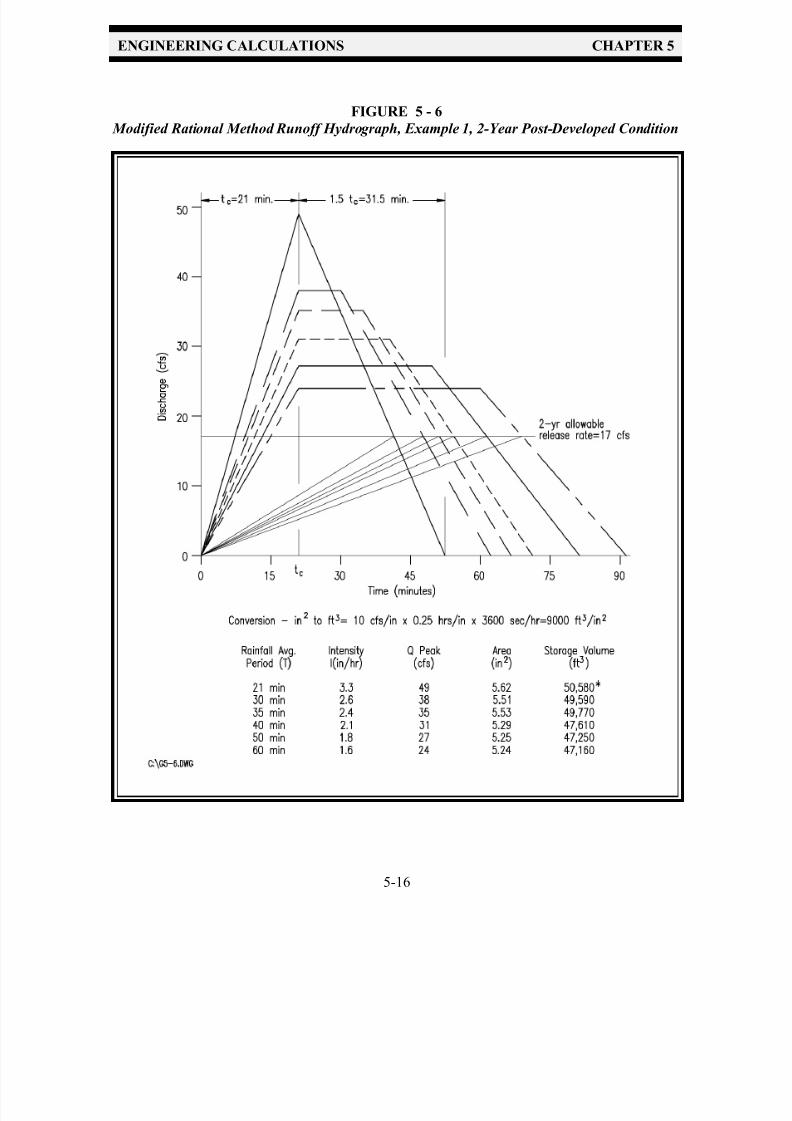
7/30/2019 Virginia Stormwater Managment Handbook Volume_II.pdf
http://slidepdf.com/reader/full/virginia-stormwater-managment-handbook-volumeiipdf 138/354

7/30/2019 Virginia Stormwater Managment Handbook Volume_II.pdf
http://slidepdf.com/reader/full/virginia-stormwater-managment-handbook-volumeiipdf 139/354

7/30/2019 Virginia Stormwater Managment Handbook Volume_II.pdf
http://slidepdf.com/reader/full/virginia-stormwater-managment-handbook-volumeiipdf 140/354

7/30/2019 Virginia Stormwater Managment Handbook Volume_II.pdf
http://slidepdf.com/reader/full/virginia-stormwater-managment-handbook-volumeiipdf 141/354
ENGINEERING CALCULATIONS CHAPTER 5
5-19
I ' a
b% T d
FIGURE 5 - 8
Trapezoidal Hydrograph Storage Volume Estimate
Rainfall Intensity
The rainfall intensity as taken from the I-D-F curves is dependent on the time of concentration, t c ,of a given watershed. Setting the storm duration, T d , equal to the time of concentration, t c , will
provide the maximum peak discharge. As stated previously, however, it does not necessarily
generate the maximum volume of discharge. Since this maximum volume of runoff is of interest,
and the storm duration is unknown, the rainfall intensity, I , must be represented as a function of time,
frequency, and location. The
relationship is expressed as follows:
Equation 5-2
Modified Rational Method Intensity, ( I ), Equation
where: I = rainfall intensity, in./hr.
T d = rainfall duration or rainfall intensity averaging period, min.
a & b = rainfall constants developed for storms of various recurrence intervals
and various geographic locations, as shown in Table 5-5
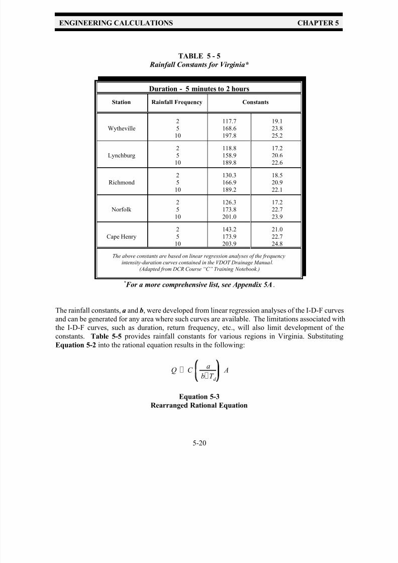
7/30/2019 Virginia Stormwater Managment Handbook Volume_II.pdf
http://slidepdf.com/reader/full/virginia-stormwater-managment-handbook-volumeiipdf 142/354
ENGINEERING CALCULATIONS CHAPTER 5
5-20
Q ' C a
b%T d
A
TABLE 5 - 5
Rainfall Constants for Virginia*
Duration - 5 minutes to 2 hours
Station Rainfall Frequency Constants
Wytheville
2
5
10
117.7
168.6
197.8
19.1
23.8
25.2
Lynchburg
2
5
10
118.8
158.9
189.8
17.2
20.6
22.6
Richmond
2
5
10
130.3
166.9
189.2
18.5
20.9
22.1
Norfolk
2
5
10
126.3
173.8
201.0
17.2
22.7
23.9
Cape Henry
2
5
10
143.2
173.9
203.9
21.0
22.7
24.8
The above constants are based on linear regression analyses of the frequency
intensity-duration curves contained in the VDOT Drainage Manual.
(Adapted from DCR Course “C” Training Notebook.)
* For a more comprehensive list, see Appendix 5A.
The rainfall constants, a and b, were developed from linear regression analyses of the I-D-F curves
and can be generated for any area where such curves are available. The limitations associated with
the I-D-F curves, such as duration, return frequency, etc., will also limit development of the
constants. Table 5-5 provides rainfall constants for various regions in Virginia. Substituting
Equation 5-2 into the rational equation results in the following:
Equation 5-3
Rearranged Rational Equation
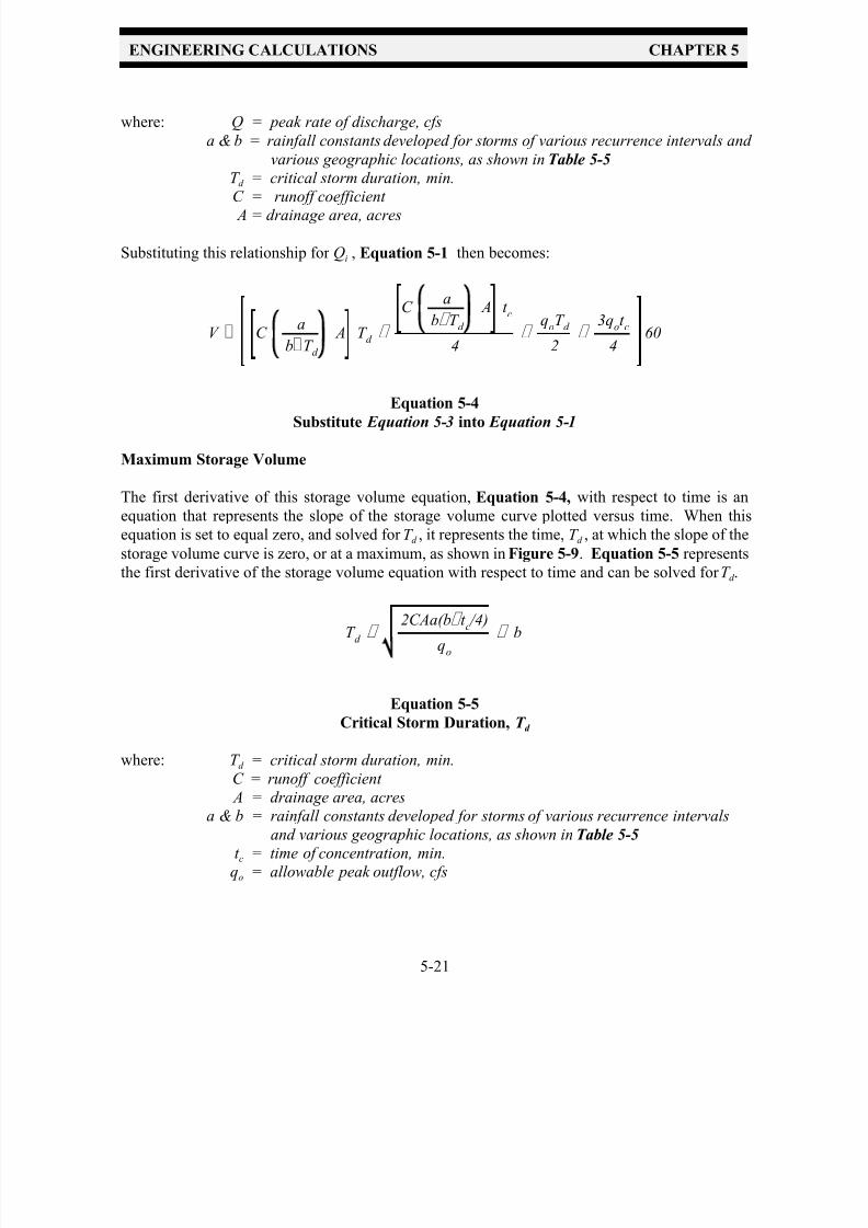
7/30/2019 Virginia Stormwater Managment Handbook Volume_II.pdf
http://slidepdf.com/reader/full/virginia-stormwater-managment-handbook-volumeiipdf 143/354
ENGINEERING CALCULATIONS CHAPTER 5
5-21
V ' C a
b%T d
A T d %
C a
b% T d
A t c
4&
qoT d
2&
3qot c
460
T d '
2CAa(b& t c /4)
qo
& b
where: Q = peak rate of discharge, cfs
a & b = rainfall constants developed for storms of various recurrence intervals and
various geographic locations, as shown in Table 5-5
T d = critical storm duration, min.
C = runoff coefficient A = drainage area, acres
Substituting this relationship for Qi , Equation 5-1 then becomes:
Equation 5-4Substitute Equation 5-3 into Equation 5-1
Maximum Storage Volume
The first derivative of this storage volume equation, Equation 5-4, with respect to time is an
equation that represents the slope of the storage volume curve plotted versus time. When this
equation is set to equal zero, and solved for T d , it represents the time, T d , at which the slope of the
storage volume curve is zero, or at a maximum, as shown in Figure 5-9. Equation 5-5 represents
the first derivative of the storage volume equation with respect to time and can be solved for T d .
Equation 5-5
Critical Storm Duration, T d
where: T d = critical storm duration, min.
C = runoff coefficient
A = drainage area, acres
a & b = rainfall constants developed for storms of various recurrence intervalsand various geographic locations, as shown in Table 5-5
t c = time of concentration, min.
qo = allowable peak outflow, cfs
7/30/2019 Virginia Stormwater Managment Handbook Volume_II.pdf
http://slidepdf.com/reader/full/virginia-stormwater-managment-handbook-volumeiipdf 144/354
ENGINEERING CALCULATIONS CHAPTER 5
5-22
FIGURE 5 - 9
Storage Volume vs. Time Curve
Equation 5-5 is solved for T d . Then, T d is substituted into Equation 5-3 to solve for Qi , and Qi is
substituted into Equation 5-1 to solve for the required storage volume. Once the storage volume
is known, the outlet structure and the stormwater facility can be sized. This method provides a
direct solution to the graphical analysis of the family of hydrographs described in Section 5-4.3 and
is quicker to use. The following procedure illustrates this method using Example 1:
Information Needed:
The Modified Rational Method-Direct Solution is similar to the previous methods since it requires
determination of the pre- and post-developed hydrology, as described in Section 4-3.1, resulting in
a pre-developed peak rate of runoff (allowable release rate) and a post-developed runoff
hydrograph. Table 5-3 provides a summary of the hydrology from Example 1. The rainfall
constants a and b for the watershed are determined from Table 5-5.

7/30/2019 Virginia Stormwater Managment Handbook Volume_II.pdf
http://slidepdf.com/reader/full/virginia-stormwater-managment-handbook-volumeiipdf 145/354
ENGINEERING CALCULATIONS CHAPTER 5
5-23
Procedure:
T d 2
' 2CAa(b& t
c /4)
qo2
& b
T d 2'
2(.59)(25.0)(130.3)(18.5& 21/4)
17 & 18.5
' 2995.9 & 18.5
T d 2
' 36 .2 min.
I 2 ' a
b% T d 2
1. Determine the 2-year critical storm duration by solving Equation 5-5:
Where, from Example 1:
= 2-year critical storm duration, min.T d 2
C = developed condition runoff coefficient = .59
A = drainage area = 25.0 acres
t c = post-developed time of concentration = 21 min.= allowable peak outflow = 17 cfs (pre-developed peak rate of q
o2
discharge)
a2 = 2-year rainfall constant = 130.3
b2 = 2-year rainfall constant = 18.5
2. Solve for the 2-year critical storm duration intensity, I 2 , using Equation 5-2 and the 2-year
critical storm duration :T d 2

7/30/2019 Virginia Stormwater Managment Handbook Volume_II.pdf
http://slidepdf.com/reader/full/virginia-stormwater-managment-handbook-volumeiipdf 146/354

7/30/2019 Virginia Stormwater Managment Handbook Volume_II.pdf
http://slidepdf.com/reader/full/virginia-stormwater-managment-handbook-volumeiipdf 147/354
ENGINEERING CALCULATIONS CHAPTER 5
5-25
T d 10
'2(.59)(25.0)(189.2)(22.1& 21/4)
24& 22.1
T d 10' 3918.6 & 22.1
T d 10' 40.5 min.
I 10
' a
b% T d 10
I 10
' 189.2
22.1 % 40.5' 3.02
Repeat Steps 2 through 4 for the 10-year storm, as follows:
5. Determine the 10-year critical storm duration , using Equation 5-5 as follows:T d 10
Where: = 10-year critical storm duration, min.T d 10
C = developed condition runoff coefficient = .59
A = drainage area = 25 acres
t c = post-developed time of concentration = 21 min.
= 24 cfsqo10
a10 = 189.2
b10 = 22.1
6. Solve for the 10-year critical storm duration intensity, I 10
, using Equation 5-2, and the 10-
year critical storm duration, .T d 10
in./hr.
7. Determine the 10-year peak inflow, , using the Rational Equation and the critical stormQi10
duration intensity I 10 :
= C I 10 AQi10
7/30/2019 Virginia Stormwater Managment Handbook Volume_II.pdf
http://slidepdf.com/reader/full/virginia-stormwater-managment-handbook-volumeiipdf 148/354
ENGINEERING CALCULATIONS CHAPTER 5
5-26
' Qi10
T d
10
% Qi10
t c
4
& qo10
T d 10
2
& 3qo10
t c
4
60
' (44.5)(40.5) % (44.5)(21)
4&
(24)(40.5)
2&
3(24)(21)
460
Where: = 10-year peak inflowQi10
C = developed condition runoff coefficient = .59
I 10 = critical storm intensity = 3.02 in./hr.
A = drainage area = 25.0 ac.
= (.59)(3.02)(25.0)Qi10
= 44.5 cfsQi10
8. Determine the required 10-year storage volume for the 10-year critical storm duration, ,T d 10
using Equation 5-1:
V 10
Where: V 10 = required storage, ft 3
= 44.5 cfsQi10
C = .59
A = 25 ac.
= 40.5 min.T d 10
t c = 21 min.
= 24 cfsqo10
V 10
V 10 = 70,308 ft 3 = 1.61 ac.ft.
V 2 and V 10 represent the total storage volume required for the 2-year and 10-year storms,
respectively. Table 5-6 provides a summary of the four different sizing procedures used in this
chapter, as applied to Example 1. The engineer should choose one of these methods based on the
complexity and size of the watershed and the chosen hydrologic method. Using the stage-storage
curve, a multi-stage riser structure can then be designed to control the appropriate storms and, if
required, the water quality volume.
7/30/2019 Virginia Stormwater Managment Handbook Volume_II.pdf
http://slidepdf.com/reader/full/virginia-stormwater-managment-handbook-volumeiipdf 149/354

7/30/2019 Virginia Stormwater Managment Handbook Volume_II.pdf
http://slidepdf.com/reader/full/virginia-stormwater-managment-handbook-volumeiipdf 150/354
ENGINEERING CALCULATIONS CHAPTER 5
5-28
Procedure:
1. Planimeter or otherwise compute the area enclosed by each contour and enter the measuredvalue into Columns 1 and 2 of Figure 5-10. The invert of the lowest control orifice represents
zero storage. This will correspond to the bottom of the facility for extended-detention or
detention facilities, or the permanent pool elevation for retention basins.
2. Convert the planimetered area (often in square inches) to units of square feet in Column 3 of
Figure 5-10.
3. Calculate the average area between each contour.
The average area between two contours is computed by adding the area planimetered for the
first elevation, column 3, to the area planimetered for the second elevation, also Column 3,and then dividing their sum by 2. This average is then written in Column 4 of Figure 5-10.
From Figure 5-10:
Average area, elevation 81-82: 0 + 1800 = 900 ft 2.
2
Average area, elevation 82-84: 1800 + 3240 = 2,520 ft 2.
2
Average area, elevation 84-86: 3240 + 5175 = 4,207 ft 2.
2
This procedure is repeated to calculate the average area found between any two consecutive
contours.
4. Calculate the volume between each contour by multiplying the average area from step 3
(Column 4) by the contour interval and placing this product in Column 6. From Figure 5-10:
Contour interval between 81 and 82 = 1 ft. x 900 ft 2 = 900 ft 3
Contour interval between 82 and 84 = 2 ft. x 2,520 ft 2 = 5,040 ft 3
This procedure is repeated for each measured contour interval.

7/30/2019 Virginia Stormwater Managment Handbook Volume_II.pdf
http://slidepdf.com/reader/full/virginia-stormwater-managment-handbook-volumeiipdf 151/354
ENGINEERING CALCULATIONS CHAPTER 5
5-29
FIGURE 5 - 10
Stage-Storage Computation Worksheet, Example 1
PROJECT: EXAMPLE 1 SHEET OF
COUNTY: COMPUTED BY: DATE:
DESCRIPTION:
ATTACH COPY OF TOPO: SCALE - 1" = 30 ft .
1 2 3 4 5 6 7 8
ELEV. AREA(in2 )
AREA(ft 2 )
AVG.
AREA
(ft 2 )
INTERVAL VOL.(ft 3 )
TOTAL VOLUME
(ft 3 ) (ac.ft .)
81 0 0 0 0900 1 900
82 2.0 1800 900 .022520 2 5040
84 3.6 3240 5940 .144207 2 8414
86 5.75 5175 14354 .337614 2 15228
88 11.17 10053 29582 .68
12991 2 2598290 17.7 15930 55564 1.2820700 2 41400
92 28.3 25470 96964 2.2331102 1 31102
93 40.8 36734 128066 2.9438105 1 38105
94 43.9 39476 166171 3.81

7/30/2019 Virginia Stormwater Managment Handbook Volume_II.pdf
http://slidepdf.com/reader/full/virginia-stormwater-managment-handbook-volumeiipdf 152/354
ENGINEERING CALCULATIONS CHAPTER 5
5-30
5. Sum the volume for each contour interval in Column 7. Using Figure 5-10, this is simply the
sum of the volumes computed in the previous step:
Contour 81, Volume = 0
Contour 82, Volume = 0 + 900 = 900 ft 3
Contour 84, Volume = 900 + 5,040 = 5,940 ft 3
Contour 86 , Volume = 5,940 + 8,414 = 14,354 ft 3
Column 8 allows for the volume to be tabulated in units of acre-feet: ft 3 ÷ 43,560 ft 2 /ac.
This procedure is then repeated for each measured contour interval.
6. Plot the stage-storage curve with stage on the y-axis versus storage on the x-axis. Figure 5-11 represents the stage-storage curve for Example 1 in units of feet (stage) versus acre-feet
(storage).
The stage-storage curve allows the designer to estimate the design high water elevation for each of
the design storms if the required storage volume has been determined. This allows for a preliminary
design of the riser orifice sizes and their configuration.
5-6 WATER QUALITY AND CHANNEL EROSION CONTROL VOLUME
CALCULATIONS
Virginia’s Stormwater Management Regulations require that the first flush of runoff, or the water quality volume, be treated to enhance water quality. The water quality volume (V wq) is the first 0.5
inches of runoff from the impervious area of development. The water quality volume must be
treated
using one or a combination of BMP's depending on the total size of the contributing watershed,
amount of impervious area, and site conditions. (Refer to Chapters 2 and 3 for BMP Selection
Criteria and BMP Minimum Standards and Specifications, respectively.)
The water quality volume is calculated as follows:
V wq (ft 3 ) = Impervious area (ft 2 ) x (½ in.) / (12 in./ft.)
V wq (ac.ft.) = V wq (ft 3 ) / 43,560 ft 2 /ac.
The water quality volume for a wet BMP may be dependent on the specific design criteria for that
BMP based on the watershed’s imperviousness or the desired pollutant removal efficiency (using
performance-based or technology-based criteria, respectively). The design criteria for each of the

7/30/2019 Virginia Stormwater Managment Handbook Volume_II.pdf
http://slidepdf.com/reader/full/virginia-stormwater-managment-handbook-volumeiipdf 153/354
ENGINEERING CALCULATIONS CHAPTER 5
5-31
BMPs, including extended-detention and retention basins, infiltration devices, constructed wetlands,
marshes, etc., are presented in Chapter 3. This discussion is focused on the calculations associated
with the control of the water quality volume in extended-detention and retention basins.
Virginia’s Stormwater Management Regulations allow for the control of downstream channelerosion by detaining a specified volume of runoff for a period of time. Specifically, 24-hour
extended detention of the runoff from the 1-year frequency storm is proposed as an alternate criteria
to the 2-year peak rate reduction specified in MS-19 of the Virginia Erosion and Sediment Control
Regulations, and the channel erosion component of the Virginia Stormwater Management
Regulations. The channel erosion control volume (V ce) is calculated by first determining the depth
of runoff (in inches) based on the fraction of rainfall to runoff (runoff curve number) and then
multiplying the runoff depth by the drainage area to be controlled. This procedure will be discussed
in 5-6.3.
FIGURE 5 - 11
Stage vs. Storage Curve, Example 1

7/30/2019 Virginia Stormwater Managment Handbook Volume_II.pdf
http://slidepdf.com/reader/full/virginia-stormwater-managment-handbook-volumeiipdf 154/354
ENGINEERING CALCULATIONS CHAPTER 5
5-32
Procedure
5-6.1 Retention Basins - Water Quality Volume
The permanent pool feature of a retention basin allows for settling of particulate pollutants, such as
sediment and other pollutants that attach adsorb to these particulates. Therefore, it is essential that
the volume of the pool be both large enough and properly configured to prevent short-circuiting .
(Short-circuiting results when runoff enters the pool and exits without sufficient time for the settling process to occur.)
The permanent pool, or “dead” storage volume, of a retention facility is a function of the water
quality volume. For example, a permanent pool sized to contain four times the water quality volume
provides greater pollutant removal capacity than a permanent pool sized to contain two times the
water quality volume. Chapter 3 provides the pollutant removal efficiencies for various permanent
pool sizes and criteria for permanent pool geometry.
Example 1 analyzes a 25-acre watershed. The water quality volume and permanent pool volume
calculations for a retention basin serving this watershed are as follows:
1. Calculate the water quality volume, V wq , for the given watershed.
From Example 1, the commercial/industrial development disturbs 11.9 acres, with 9.28 acres
(404,236 ft 2.) of impervious cover after development.
V wq = 404,236 ft 2 x ½ in. / 12 in./ft.
= 16,843 ft 3
= 16,843 ft 3 /43,560 ft 2 /ac.
V wq = 0.38 ac.ft.
2. Size the permanent pool based on the desired pollutant removal efficiency or the drainage
area impervious cover .
The pool volume will be sized based upon the desired pollutant removal efficiency. Referring
to Table 3.06-1, the permanent pool must be sized for 4 x V wq for a pollutant removal
efficiency of 65%.
Permanent Pool Volume = V wq x 4.0
Permanent Pool Volume = 0.38 ac.ft. x 4.0 = 1.52 ac.ft.

7/30/2019 Virginia Stormwater Managment Handbook Volume_II.pdf
http://slidepdf.com/reader/full/virginia-stormwater-managment-handbook-volumeiipdf 155/354
ENGINEERING CALCULATIONS CHAPTER 5
5-33
5-6.2 Extended-Detention Basins - Water Quality Volume and Orifice Design
A water quality extended-detention basin treats the water quality volume by detaining it and releasing
it over a specified amount of time. In theory, extended-detention of the water quality volume will allow
the particulate pollutants to settle out of the first flush of runoff, functioning similarly to a permanent pool. Virginia’s Stormwater Management Regulations pertaining to water quality specify a 30-hour draw
down time for the water quality volume. This is a brim draw down time, beginning at the time of peak
storage of the water quality volume. Brim-draw down time means the time required for the entire
calculated volume to drain out of the basin. This assumes that the brim volume is present in the basin
prior to any discharge. In reality, however, water is flowing out of the basin prior to the full or brim
volume being reached. Therefore, the extended detention orifice can be sized using either of the
following methods:
1. Use the maximum hydraulic head associated with the water quality volume (V wq) and calculate the
orifice size needed to achieve the required draw down time, and route the the water quality volume
through the basin to verify the actual storage volume used and the drawdown time.
2. Approximate the orifice size using the average hydraulic head associated with the water quality
volume (V wq) and the required draw down time.
The two methods for calculating the required size of the extended detention orifice allow for a quick and
conservative design (Method 2 above) and a similarly quick estimation with a routing to verify the
performance of the design (Method 1).
Method 1, which uses the maximum hydraulic head and maximum discharge in the calculation, results
in a slightly larger orifice than the same procedure using the average hydraulic head (Method 2). The
routing allows the designer to verify the performance of the calculated orifice size. As a result of therouting effect however, the actual basin storage volume used to achieve the draw down time will be less
than the computed brim draw down volume. It should be noted that the routing of the extended detention
of the runoff from storms larger than the water quality storm (such as the 1-year frequency storm for
channel erosion control) will result in proportionately larger reduction in the actual storage volume
needed to achieve the required extended detention. (Refer to Section 5-6.3 for the extended detention
design procedures for channel erosion protection.)
The procedure used to size an extended detention orifice includes the first steps of the design of a multi-
stage riser for a basin controlling water quality and/or channel erosion, and peak discharge. These steps
are repeated for sizing the 2-year and 10-year release openings. Other design storms may be used as
required by ordinance or downstream conditions.
Method 1: Water quality orifice design using maximum hydraulic head and routing of the water
quality volume.
A water quality extended-detention basin sized for two times the water quality volume will be used here
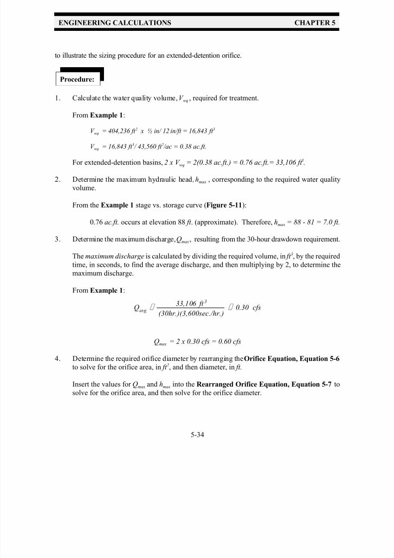
7/30/2019 Virginia Stormwater Managment Handbook Volume_II.pdf
http://slidepdf.com/reader/full/virginia-stormwater-managment-handbook-volumeiipdf 156/354
ENGINEERING CALCULATIONS CHAPTER 5
5-34
Procedure:
Qavg
' 33,106 ft 3
(30hr.)(3,600sec./hr.)' 0.30 cfs
to illustrate the sizing procedure for an extended-detention orifice.
1. Calculate the water quality volume, V wq , required for treatment.
From Example 1:
V wq = 404,236 ft 2 x ½ in/ 12 in/ft = 16,843 ft 3
V wq = 16,843 ft 3 / 43,560 ft 2 /ac = 0.38 ac.ft.
For extended-detention basins, 2 x V wq = 2(0.38 ac.ft.) = 0.76 ac.ft.= 33,106 ft 3.
2. Determine the maximum hydraulic head, hmax , corresponding to the required water quality
volume.
From the Example 1 stage vs. storage curve (Figure 5-11):
0.76 ac.ft. occurs at elevation 88 ft . (approximate). Therefore, hmax = 88 - 81 = 7.0 ft.
3. Determine the maximum discharge, Qmax, resulting from the 30-hour drawdown requirement.
The maximum discharge is calculated by dividing the required volume, in ft 3, by the required
time, in seconds, to find the average discharge, and then multiplying by 2, to determine the
maximum discharge.
From Example 1:
Qmax = 2 x 0.30 cfs = 0.60 cfs
4. Determine the required orifice diameter by rearranging the Orifice Equation, Equation 5-6
to solve for the orifice area, in ft 2, and then diameter, in ft.
Insert the values for Qmax and hmax into the Rearranged Orifice Equation, Equation 5-7 to
solve for the orifice area, and then solve for the orifice diameter.
7/30/2019 Virginia Stormwater Managment Handbook Volume_II.pdf
http://slidepdf.com/reader/full/virginia-stormwater-managment-handbook-volumeiipdf 157/354
ENGINEERING CALCULATIONS CHAPTER 5
5-35
a ' 0.6
0.6 (2)(32.2)(7.0)
a ' 0.047 t 2 ' π r 2 ' π d 2 /4
d ' 4a
π '
4(0.047 ft 2 )
π
Q ' Ca 2 gh a 'Q
C 2 gh
Equation 5-6 Equation 5-7
Orifice Equation Rearranged Orifice Equation
where: Q = discharge, cfs
C = dimensionless coefficient = 0.6
a = area of the orifice, ft 2
g = gravitational acceleration, 32.2 ft/sec2
h = head, ft.
From Example 1: For orifice area:
For orifice diameter:
d = orifice diameter = 0.245 ft = 2.94"
Use a 3-inch diameter water quality orifice.
Routing the water quality volume (V wq) of 0.76 ac.ft., occurring at elevation 88 feet, through a 3-
inch water quality orifice will allow the designer to verify the draw down time, as well as the
maximum elevation of 88 feet.
Route the water quality volume.
This calculation will give the engineer the inflow-storage-outflow relationship in order to verify the
actual storage volume needed for the extended detention of the water quality volume. The routing
procedure takes into account the discharge that occurs before maximum or brim storage of the water
quality volume, as opposed to the brim drawdown described in Method 2. The routing procedure
is simply a more accurate analysis of the storage volume used while water is flowing into and outof the basin. Therefore, the actual volume of the basin used will be less than the volume as defined
by the regulation. This procedure will come in handy if the site to be developed is tight and the area
needed for the stormwater basin must be “squeezed” as much as possible.

7/30/2019 Virginia Stormwater Managment Handbook Volume_II.pdf
http://slidepdf.com/reader/full/virginia-stormwater-managment-handbook-volumeiipdf 158/354
ENGINEERING CALCULATIONS CHAPTER 5
5-36
Procedure (contd.):
'
Q ' 0.6 (.047 ) (2)(32.2)(h)
Q ' 0.22 h
The routing effect of water entering and discharging from the basin simultaneously will also result
in the actual drawdown time being less than the calculated 30 hours. Judgement should be used to
determine whether the orifice size should be reduced to achieve the required 30 hours or if the actual
time achieved will provide adequate pollutant removal.
NOTE: The designer will notice a significant reduction in the actual storage volume used when
routing the extended detention of the runoff from the 1-year frequency storm (channel erosion
control). Please refer to Chapter 5-6.3 and Chapter 5-11 for the appropriate design procedures
when extended detention is provided for channel erosion control.
Routing the water quality volume depends on the ability to work backwards from the design runoff
volume of 0.5 inches to find the rainfall amount. Using SCS methods, the rainfall needed to
generate 0.5 inches of runoff from an impervious surface ( RCN=98) is 0.7 inches. The SCS design
storm is the Type II, 24-hour storm. Therefore, the water quality storm using SCS methods is
defined as the SCS Type II, 24-hour storm, with a rainfall depth = 0.7 inches.
The rational method does not provide a design storm derived from a specified rainfall depth. Its
rainfall depth depends on the storm duration (watershed t c) and the storm return frequency. Since
the water quality storm varies with runoff amount, not the design storm return frequency, an
input runoff hydrograph representing the water quality volume cannot be generated using
rational method parameters. Therefore Method 1, routing of the water quality volume, must use
SCS methods. See Chapter 4 for details on SCS methods.
Continuing with Example 1, the procedure is as follows:
5. Calculate a stage-discharge relationship using the Orifice Equation, Equation 5-6 and the
orifice size determined in Step 4.
From Example 1, using the 3-inch diameter orifice, the calculation is as follows:
Orifice Equation 5-6
where: h = water surface elevation minus the orifice’s centerline elevation*, in ft.
7/30/2019 Virginia Stormwater Managment Handbook Volume_II.pdf
http://slidepdf.com/reader/full/virginia-stormwater-managment-handbook-volumeiipdf 159/354
ENGINEERING CALCULATIONS CHAPTER 5
5-37
*Note: If the orifice size is small relative to the anticipated head, h, values of h may bedefined as the water surface elevation minus the invert of the orifice elevation.
7. Complete a stage-discharge table for the range of elevations in the basin, as shown in
Table 5-7:
TABLE 5 - 7
Stage-Discharge Table: Water Quality Orifice Design
Elevation h ( ft ) Q (cfs)
81 0 0
82 1 0.2
83 2 0.3
84 3 0.4
85 4 0.4
86 5 0.5
87 6 0.5
88 7 0.6
8. Determine the time of concentration as defined in Chapter 4 for the impervious area.
From Example 1, the developed time of concentration, t c = 0.46 hours. The impervious
area time of concentration, = 0.09 hours, or 5.4 minutes.t cimp
9. Using , the stage-discharge relationship, the stage-storage relationship, and the impervioust cimp
acreage ( RCN = 98), route the water quality storm through the basin. The water quality storm
for this calculation is the SCS Type 2, 24-hour storm, rainfall depth = 0.7 inches. (Note that
the rainfall depth is established as the amount of rainfall required to generate 0.5 inches of
runoff from the impervious area.)
The water quality volume may be routed using a variety of computer programs such as TR-20,
HEC-1, or other storage indication routing programs. Alternatively, it can be routed by hand
using the storage indication routing procedure outlined in Section 5-9 of this chapter.

7/30/2019 Virginia Stormwater Managment Handbook Volume_II.pdf
http://slidepdf.com/reader/full/virginia-stormwater-managment-handbook-volumeiipdf 160/354
ENGINEERING CALCULATIONS CHAPTER 5
5-38
10. Evaluate the discharge hydrograph to verify that the drawdown time from maximum storage
to zero discharge is at least 30 hours. (Note that the maximum storage corresponds to the
maximum rate of discharge on the discharge hydrograph.)
The routing of the water quality volume using TR-20 results in a maximum storage elevationis 85.69 ft. versus the approximated 88.0 ft. The brim drawdown time is 17.5 hours (peak
discharge occurs at 12.5 hours and .01 discharge occurs at 30 hours). For this example, the
orifice size may be reduced to provide a more reasonable drawdown time and another routing
performed to find the new water quality volume elevation.
METHOD 2: Water quality orifice design using average hydraulic head and average discharge.
The procedure described in Method 2 is presented in the next section. For the previous example,
Method 2 results in a 2.5 inch orifice (versus a 3.0 inch orifice), and the design extended detention
water surface elevation is set at 88 ft.(versus 85.69ft.). ( It should be noted that trial two of Method
1 as noted above may result in a design water surface elevation closer to 88 ft.) If the basin is to
control additional storms, such as the 2-year and/or 10-year storms, the additional storage volume
would be "stacked" just above the water quality volume. The invert for the 2-year control, for
example, would be set at 88.1 ft.
5-6.3 Extended-Detention Basins - Channel Erosion Control Volume and Orifice Design
Extended detention of a specified volume of stormwater runoff can also be incorporated into a basin
design to protect downstream channels from erosion. Virginia’s Stormwater Management
Regulations recommend 24-hour extended detention of the runoff from the 1-year frequency storm
as an alternative to the 2-year peak rate reduction required by MS-19 of the Virginia Erosion and
Sediment Control Regulations. A full discussion of this channel erosion criteria will be presented
in a future Technical Bulletin, along with practical guidance from DCR on the effective
implementation of the criteria. The discussion presented here is for the design of a channel erosion
control extended-detention orifice.
The design of a channel erosion control extended-detention orifice is similar to the design of the
water quality orifice in that two methods can be employed:
1. Use the maximum hydraulic head associated with the specified channel erosion control(V ce) storage volume and calculate the orifice size needed to achieve the required drawdown time and route the 1-year storm through the basin to verify the storage volume andthe draw down time, or
2. Approximate the orifice size using the average hydraulic head associated with the
channel erosion control volume (V ce) and draw down time.

7/30/2019 Virginia Stormwater Managment Handbook Volume_II.pdf
http://slidepdf.com/reader/full/virginia-stormwater-managment-handbook-volumeiipdf 161/354
ENGINEERING CALCULATIONS CHAPTER 5
5-39
Procedure
The routing procedure takes into account the discharge that occurs before maximum or brim storage
of the channel erosion control volume (V ce). The routing procedure simply provides a more accurate
accounting of the storage volume used while water is flowing into and out of the basin, and results
in less storage volume being used than the calculated brim storage volume associated with the
maximum hydraulic head. The actual storage volume needed for extended detention of the runoff generated by the 1-year frequency storm will be approximately 60 percent of the calculated volume
(V ce) of runoff for curve numbers between 75 and 95 and time of concentration between 0.1 and 1
hour.
The following procedure illustrates the design of the extended-detention orifice for channel erosion
control. Refer to Chapter 6 for Example 6.2 which includes the design of an extended-detention
orifice for channel erosion control, Method 1, within the design of a multi-stage riser.
Method 2:
1. Calculate the channel erosion control volume, V ce.
Determine the rainfall amount (inches) of the 1-year frequency storm for the local area where
the project is located (Appendix 4B). With the rainfall amount and the runoff curve number
(RCN), determine the corresponding runoff depth using the runoff Equation (Chapter 4:
Hydrologic Methods - SCS TR-55) or the Rainfall - Runoff Depth Charts (Appendix 4C).
From Example 2:
1-year rainfall = 2.7 inches, RCN = 75; using Appendix 4C, the 1-year frequency depth of runoff =
0.8 inches, therefore:
V ce = 25 ac. x 0.8 in. × 1'/12" = 1.66 ac.ft.
To account for the routing effect, reduce the channel erosion control volume:
V ce = (0.6)(1.66 ac.ft.) = 1.0 ac.ft. = 43,560 ft.3
2. Determine the average hydraulic head , havg , corresponding to the required channel erosion
control volume.
From Example 2 - Stage - Storage Curve: 1.0 ac.ft. occurs at elevation 89.0 ft. Therefore,
havg = (89 - 81) / 2 = 4.0 ft.

7/30/2019 Virginia Stormwater Managment Handbook Volume_II.pdf
http://slidepdf.com/reader/full/virginia-stormwater-managment-handbook-volumeiipdf 162/354
ENGINEERING CALCULATIONS CHAPTER 5
5-40
Qavg
' 43,560 ft 3
(24hr.)(3,600sec./hr.)' 0.5 cfs
a ' 0.5
0.6 (2)(32.2)(4.0)
a ' 0.052 t 2 ' π r 2 ' π d 2 /4
d '
4a
π '
4(0.052 ft 2 )
π
3. Determine the average discharge, Qavg , resulting from the 24-hour draw down requirement.
The average discharge is calculated by dividing the required volume, in ft 3, by the required
time, in seconds, to find the average discharge.
From Example 2:
4. Determine the required orifice diameter by rearranging the Orifice Equation, Equation 5-6
to solve for the orifice area, in ft 2, and then diameter, in ft.
Insert the values for Qavg and havg into the Rearranged Orifice Equation, Equation 5-7 to
solve for the orifice area, and then solve for the orifice diameter.
Q ' Ca 2 gh a 'Q
C 2 gh
Equation 5-6 Equation 5-7Orifice Equation Rearranged Orifice Equation
where: Q = discharge, cfsC = dimensionless coefficient = 0.6 a = area of the orifice, ft 2
g = gravitational acceleration, 32.2 ft/sec2
h = head, ft.
From Example 2: For orifice area:
For orifice diameter:
d = orifice diameter = 0.257 ft = 3.09 inches
Use 3.0-inch diameter channel erosion extended detention orifice

7/30/2019 Virginia Stormwater Managment Handbook Volume_II.pdf
http://slidepdf.com/reader/full/virginia-stormwater-managment-handbook-volumeiipdf 163/354
ENGINEERING CALCULATIONS CHAPTER 5
5-41
The use of Method 1, utilizing the maximum hydraulic head and a routing of the 1-year storm is
illustrated in Chapter 6: Example 6.2. Methd 1 results in a 3.7" diameter orifice and a routed water
surface elevation of 88.69 ft. Additional storms to may be “stacked” just above this volume if
additional controls are desired.
5-7 MULTI-STAGE RISER DESIGN
A principal spillway system that controls the rate of discharge from a stormwater facility will often
use a multi-stage riser for the drop inlet structure.
A multi-stage riser is a structure that incorporates separate openings or devices at different
elevations to control the rate of discharge from a stormwater basin during multiple design storms.
Permanent multi-stage risers are typically constructed of concrete to help increase their life
expectancy; they can be precast or cast-in-place. The geometry of risers will vary from basin to
basin. The engineer can be creative to provide the most economical and hydraulically efficient riser
design possible. Figure 3-02.1 in Chapter 3 provides some examples of multi-stage riser structures.
In a stormwater management basin design, the multi-stage riser is of utmost importance since it
controls the design water surface elevations. In designing the multi-stage riser, many iterative
routings are usually required to arrive at a minimum structure size and storage volume that provides
proper control. Each iterative routing requires that the facility’s size ( stage-storage curve) and
outlet shape ( stage-discharge table or rating curve) be designed and tested for performance. Prior
to final design, it is helpful to approximate the required storage volume and outlet shape using one
of the “shortcut” methods, as described in Section 5-4. In doing this, the number of iterations may
be reduced. The following procedures outline methods for approximating and then completing the
design of a riser structure. (These design procedures are illustrated in the examples found in
Chapter 6.)
Information needed:
1. The hydrology for the watershed or drainage area to be controlled, calculated by using one
of the methods outlined in Chapter 4, and
2. The allowable release rates for the facility, as established by ordinance or downstream
conditions.
The design procedure provided here will incorporate the traditional 2-year and 10-year design
storms and the pre-developed hydrology will establish the allowable discharge rates of the

7/30/2019 Virginia Stormwater Managment Handbook Volume_II.pdf
http://slidepdf.com/reader/full/virginia-stormwater-managment-handbook-volumeiipdf 164/354
ENGINEERING CALCULATIONS CHAPTER 5
5-42
Procedure:
developed watershed. It should be noted that any design storm, 1-year, 5-year, etc., can be
substituted into this design procedure, as required.
STEP 1 Determine Water Quality or Extended Detention Requirements
Calculate the water quality volume and decide what method (extended-detention or retention) will
be used to treat it, and/or calculate the channel erosion control volume for extended-detention, if
required. (Virginia’s Stormwater Management Regulations state that the water quality volume is
equal to the first 0.5 inch of runoff multiplied by the total impervious area of the land
development project, and that the channel erosion control volume for extended detention is
the runoff generated by the site during the 1-year frequency storm .)
a. Water Quality Extended-Detention Basin: The water quality volume must be detained and released
over 30-hours. The established pollutant removal efficiency is based on a 30-hour drawdown.
b. Water Quality Retention Basin: The volume of the permanent pool is established by the site
impervious cover or the desired pollutant removal efficiency.
c. Channel Erosion Control Extended-Detention Basin: The channel erosion control volume must be
detained and released over 24 hours.
Refer to Chapter 3 for minimum BMP design standards and details.
STEP 2 Compute Allowable Release Rates
Compute the pre- and post-developed hydrology for the watershed. Sometimes, the pre-developed
hydrology will establish the allowable release rate from the basin. Other times, the release rate will
be established by downstream conditions. In either case, the post-developed hydrology will provide
the peak inflow into the basin, as a peak rate (cfs) or a runoff hydrograph. Refer to Section 5-3,
Allowable Release Rates.
STEP 3 Estimate the Required Storage Volume
Estimate the storage volume required using one of the “shortcut” volume estimate methods
described in Section 5-4. The information required includes the developed condition peak rate of
runoff, or runoff hydrograph, and the allowable release rates for each of the appropriate design
storms.

7/30/2019 Virginia Stormwater Managment Handbook Volume_II.pdf
http://slidepdf.com/reader/full/virginia-stormwater-managment-handbook-volumeiipdf 165/354
ENGINEERING CALCULATIONS CHAPTER 5
5-43
STEP 4 Grade the Basin; Create Stage-Storage Curve
After considering the site geometry and topography, select a location for the proposed stormwater
management basin. By trial and error, size the basin such that it will hold the approximate required
storage volume. Ensure that the storage volume is measured from the lowest stage outlet. (Note: thestorage volume can be computed by planimetering the contours and creating a stage-storage
relationship as described in Section 5-5.) Remember that this is a preliminary sizing which needs
to be fine-tuned during the final design.
STEP 5a Design Water Quality Orifice (Extended-Detention)
The procedure for sizing the water quality orifice for an extended-detention basin is covered in
Section 5-6.2 of this chapter. Using either Method 1 or Method 2, the designer establishes the size
of the water quality or stream channel erosion control orifice and the design maximum water surface
elevation.
The lowest stage outlet of an extended-detention basin is the invert of the extended-detention (or
water quality) orifice, which corresponds to zero storage. Section 5-6.2 provides a detailed
discussion for sizing the water quality orifice and Chapter 6 gives examples of the calculation
procedure.
STEP 5b Set Permanent Pool Volume (Retention)
In a retention pond, the permanent pool volume, from STEP 1, establishes the lowest stage outlet
for the riser structure (not including a pond drain, if provided). The permanent pool elevation,
therefore, corresponds to “0” storage for the design of the “dry” storage volume stacked on top of
the permanent pool.
STEP 6 Size 2-Year Control Orifice
(The 2-year storm is used here to show the design procedure. Other design storms or release
requirements can be substituted into the procedure.)
Knowing the 2-year storm storage requirement, from design STEP 3, and the water quality volume,
from design STEP 1, the engineer can do a preliminary design for the 2-year release opening in the
multi-stage riser. To complete the design, some iterations may be required to meet the allowable
release rate performance criteria. This procedure is very similar to the water quality orifice sizing
calculations:
1. Approximate the 2-year maximum head, .h2max
Establish the approximate elevation of the 2-year maximum water surface elevation using the stage-
7/30/2019 Virginia Stormwater Managment Handbook Volume_II.pdf
http://slidepdf.com/reader/full/virginia-stormwater-managment-handbook-volumeiipdf 166/354
ENGINEERING CALCULATIONS CHAPTER 5
5-44
storage curve and the preliminary sizing calculations. Subtract the water quality volume elevation
from the approximate 2-year maximum water surface elevation to find the 2-year maximum head,
. If there are no water quality requirements, use the elevation of the basin bottom or invert.h2max
2. Determine the maximum allowable 2-year discharge rate, , from STEP 2.Q2allowable
3. Calculate the size of the 2-year control release orifice using the Rearranged Orifice
Equation, Equation 5-7 and solve for the area, a, in ft 2.
The engineer may choose to use any one of a variety of orifice shapes or geometries. Regardless
of the selection, the orifice will initially act as a weir until the top of the orifice is submerged.
Therefore, the discharges for the first stages of flow are calculated using the weir equation:
Qw = C w L h1.5
Equation 5-8
Weir Equation
where: Qw = weir flow discharge, cfs
C w = dimensionless weir flow coefficient, typically equal to 3.1
for sharp crested weirs. Refer to Table 5-8.
L = length of weir crest, ft.
h = head, ft., measured from the water surface elevation to the
crest of the weir
Flow through the rectangular opening will transition from weir flow to orifice flow once the water surface has
risen above the top of the opening. This orifice flow is expressed by the orifice equation. The area, a, of a
rectangular orifice is written as a = L x H ,
where: L = length of opening, ft.
H = height of opening, ft.
Figure 5-12 shows a rectangular orifice acting as a weir at the lower stages and as an orifice after the water
surface rises to height H , the height of the opening.
4. Develop the stage-storage-discharge relationship for the 2-year storm.
Calculate the discharge using the orifice equation and, if a rectangular opening is used, the weir
equation as needed for each elevation specified on the stage-storage curve. Record the dischargeon a Stage-Storage-Discharge Worksheet. Figure 5-13 shows a completed Stage-Storage-Discharge
Worksheet for Example 2. A blank worksheet is provided in Appendix 5D.

7/30/2019 Virginia Stormwater Managment Handbook Volume_II.pdf
http://slidepdf.com/reader/full/virginia-stormwater-managment-handbook-volumeiipdf 167/354
ENGINEERING CALCULATIONS CHAPTER 5
5-45
FIGURE 5 - 12
Weir and Orifice Flow
STEP 7 Check Performance of 2-Year Opening
(Note: This step may not be necessary if the design is to be completed using one of the shortcutrouting procedures where the water surface elevations are established by the required storage
volume and not by an actual routing.)
1. Check the performance of the 2-year control opening by a) reservoir routing the 2-year storm
through the basin using an acceptable reservoir routing computer programor by b) doing the
long hand calculations outlined in Section 5-9 of this chapter . Verify that the 2-year release
rate is less than or equal to the allowable release rate. If not, reduce the size of the opening
or provide additional storage and repeat STEP 6.
This procedure presents just one of many riser configurations. The engineer may choose to use any
type of opening geometry for controlling the design storms and, with experience, may come torecognize the most efficient way to configure the riser. Note that if a weir is chosen for the 2-year
storm control, the procedures outlined here for the 10-year storm may be used by substituting with
the appropriate values for the 2-year storm. Refer to Figure 3-02.1 for several different riser shapes.
7/30/2019 Virginia Stormwater Managment Handbook Volume_II.pdf
http://slidepdf.com/reader/full/virginia-stormwater-managment-handbook-volumeiipdf 168/354
ENGINEERING CALCULATIONS CHAPTER 5
5-46
The 10-year control invert may be set at a small distance, such as 0.1 feet minimum,above the 2-year maximum water surface elevation. If the 2-year orifice is also to beused for the 10-year control, the head is measured from the maximum water surfaceelevation to the centerline of the 2-year orifice. See Figure 5-14.
STEP 8 Size 10-Year Control Opening
The design of the 10-year storm control opening is similar to the procedure used in sizing the 2-year
control opening:
1. From the routing results, identify the exact 2-year water surface elevation.
2. Set the invert of the 10-year control just above the 2-year design water surface elevation and
determine the corresponding storage volume from the stage-storage curve. Add this elevation,
storage, and 2-year discharge to the stage-storage-discharge worksheet, Figure 5-13.
3. Establish the approximate 10-year maximum water surface elevation using the stage-storage
curve and the preliminary sizing calculations. Subtract the invert elevation of the 10-year
control (from Step 2 above) from the approximate 10-year maximum water surface elevation
to find the 10-year maximum head, .h10max
4. Determine the maximum allowable 10-year discharge rate, , from STEP 2.Q10allowable
5. Calculate the required size of the 10-year release opening. The engineer may choose between
a circular and rectangular orifice, or a weir. If a weir is chosen, the weir flow equation can be rearranged to solve for L as follows.
QW = C W L h1.5 L = / C W h1.5 Q
10allowable
Equation 5-8 Equation 5-9
Weir Equation Rearranged Weir Equation
Where: L = length of weir required, ft.
C W = dimensionless weir flow coefficient, see Table 5-8
= 10-year allowable riser weir discharge, cfsQ10allowable
h = hydraulic head; water surface elevation minus the weir crest elevation
6. Develop the stage-storage-discharge relationship for the 10-year storm. Calculate the
discharge for each elevation specified on the stage-storage curve, and record the discharge
on a Stage-Storage-Discharge Worksheet, as shown in Figure 5-13.

7/30/2019 Virginia Stormwater Managment Handbook Volume_II.pdf
http://slidepdf.com/reader/full/virginia-stormwater-managment-handbook-volumeiipdf 169/354
ENGINEERING CALCULATIONS CHAPTER 5
5-47
Any weir length lost to the trash rack or debris catcher must be accounted for.
See Chapter 3 for Trash Rack Specifications and example riser configurations.
TABLE 5 - 8
Weir Flow Coefficients
WEIR FLOW COEFFICIENTS, C
Measured head, h,
( ft.)
Breadth of weir crest
( ft.)
0.50 0.75 1.00
0.2
0.4
0.6
0.8
1.0
1.2
1.4
1.6
1.8
2.0
3.0
4.0
5.0
2.80
2.92
3.08
3.30
3.32
3.32
3.32
3.32
3.32
3.32
3.32
3.32
3.32
2.75
2.80
2.89
3.04
3.14
3.20
3.26
3.29
3.32
3.32
3.32
3.32
3.32
2.69
2.72
2.75
2.85
2.98
3.08
3.20
3.28
3.31
3.30
3.32
3.32
3.32
Source: Kings Handbook of Hydraulics
STEP 9 Check Performance of 10-Year Opening
(Note: This step may not be necessary if the design is to be completed using one of the short-cutrouting procedures where the water surface elevations are established by the required storage
volume and not by an actual routing.)

7/30/2019 Virginia Stormwater Managment Handbook Volume_II.pdf
http://slidepdf.com/reader/full/virginia-stormwater-managment-handbook-volumeiipdf 170/354
7/30/2019 Virginia Stormwater Managment Handbook Volume_II.pdf
http://slidepdf.com/reader/full/virginia-stormwater-managment-handbook-volumeiipdf 171/354
ENGINEERING CALCULATIONS CHAPTER 5
5-49
be accomplished by checking the flow rates for the riser weir, riser orifice, and barrel inlet and outlet
flow control at each stage of discharge. The lowest discharge for any given stage will be the
controlling flow.
The following procedures are for designing and checking riser and barrel system hydraulics.a. Riser Flow Control
During the design of the control orifices and riser weir, the geometry of the riser is
established. Subsequently, the riser must be checked to determine at what stage it transitions
from riser weir to riser orifice flow control. The riser weir controls the flow initially, and then
as the water rises, the top of the riser acts as a submerged horizontal orifice. Thus, the flow
transitions from riser weir flow control to riser orifice flow control as the water in the basin
rises. The flow capacity of the riser weir is determined using the Weir Equation, Equation
5-8, and the flow capacity of the riser orifice is determined using the Orifice Equation,
Equation 5-6, for each elevation. The smaller of the two flows for any given elevation isthe controlling flow.
1. Calculate the flow, in cfs, over the riser weir using the standard Weir Equation, Equation 5-8,
for each elevation specified on the Stage-Storage-Discharge Worksheet, Figure 5-13. Record
the flows on the worksheet.
The weir length, L, is the circumference or length of the riser structure, measured at the crest,
less any support posts or trash rack. The head is measured from the water surface elevation
to the crest of the riser structure (refer to Figure 5-14).
2. Calculate the flow, in cfs, through the riser structure using the standard Orifice Equation,
Equation 5-6, for each elevation specified on the Stage-Storage-Discharge Worksheet, Figure
5-13. Record the flows on the worksheet.
The Orifice flow area , a, is measured from the inside dimensions of the riser structure. The
head is measured from the water surface elevation to the elevation of the orifice centerline,
or, since the orifice is horizontal, to the elevation of the riser crest.
3. Compare the riser weir flow discharges to the riser orifice flow discharges. The smaller of the
two discharges is the controlling flow for any given stage.
b. Barrel Flow Control
Two types of barrel flow exist: 1) barrel flow with inlet control , as shown in Figure 5-15c,
and 2) barrel flow with outlet, or pipe flow control , as shown in Figure 5-15d. For both
types, different factors and formulas are used to compute the hydraulic capacity of the barrel.
During barrel inlet flow control, the diameter of the barrel, amount of head acting on the
7/30/2019 Virginia Stormwater Managment Handbook Volume_II.pdf
http://slidepdf.com/reader/full/virginia-stormwater-managment-handbook-volumeiipdf 172/354
ENGINEERING CALCULATIONS CHAPTER 5
5-50
The inlet control nomographs are not truly representative of barrel inlet flow. These nomographs
should be used carefully and with the understanding that they were developed to predict flow
through highway culverts operating under inlet control. However, depending on the size
relationship between the riser and outlet conduit, the inlet control nomograph may provide a
barrel, and the barrel entrance shape play a part in controlling the flow. For barrel outlet, or
pipe flow, control, consideration is given to the length, slope, and roughness of the barrel, and
the elevation of the tailwater, if any, in the outlet channel.
1. Barrel Inlet Flow Control
Barrel inlet flow control means that the capacity of the barrel is controlled at the barrel
entrance by the depth of headwater and the barrel entrance, which is acting as a submerged
orifice. The flow through the barrel entrance can be calculated using the Orifice Equation,
Equation 5-6, or by simply using the Pipe Flow Nomograph shown in Figure 5-16. This
nomograph provides stage-discharge relationships for concrete culverts of various sizes.
[Additional nomographs for other pipe materials and geometrics are available; refer to the
U.S. Bureau of Public Roads (BPR) Hydraulic Engineering Circular (H.E.C.) 5.] The
headwater , or depth of ponding, is the vertical distance measured from the water surface
elevation to the invert at the entrance to the barrel. Refer to Figure 5-16 for ratios of
headwater to pipe diameter , or HW/D. This nomograph, based on the orifice equation, provides flow rates for three possible hydraulic entrance shapes, as shown in Figure 5-17.
During barrel inlet flow control, neither the barrel’s length nor its outlet conditions are factors
in determining the barrel’s capacity. Note that when the HW/D design values exceed the chart
values, the designer may use the orifice equation (Equation 5-6) to solve for the flow rate.
The following procedure outlines the steps to calculate the discharge during barrel inlet flow control
conditions:
1. Determine the entrance condition of the barrel (see Figure 5-17).
2. Determine the headwater to pipe diameter ratio ( HW/D) for each elevation specified on
the stage-storage-discharge worksheet. Headwater is measured from the water surface
elevation to the upstream invert of the barrel (see Figures 5-14 and 5-18).
3. Determine the discharge, Q, in cfs, using the inlet control nomograph for circular concrete pipe presented in Figure 5-16 (or the BPR H.E.C. 5 pipe flow nomographs for
other pipe materials), or the Orifice Equation, Equation 5-6 (for HW/D values which
exceed the range of the nomographs) for each elevation specified on the Stage-Storage-
Discharge Worksheet. Enter the values on the worksheet.

7/30/2019 Virginia Stormwater Managment Handbook Volume_II.pdf
http://slidepdf.com/reader/full/virginia-stormwater-managment-handbook-volumeiipdf 173/354
ENGINEERING CALCULATIONS CHAPTER 5
5-51
Q ' a2gh
1% K m% K p L
2. Barrel Outlet Flow Control
Barrels flowing under outlet or pipe flow control experience full flow for all or part of the
barrel length, as shown in Figure 5-15d.
The general pipe flow equation is derived by using the Bernouli and Continuity Principles and is
simplified to:
Equation 5 - 10
Pipe Flow Control Equation
Where: Q = discharge, cfs
a = flow area of the barrel, ft 2
g = acceleration due to gravity, ft./sec2
h = elevation head differential, ft., see Figure 5-18
K m = coefficient of minor losses: K e + K b K e = entrance loss coefficient, see Table 5-9
K b = bend loss coefficient, typically = 0.5 for riser and barrel system
K p = coefficient of pipe friction, see Table 5-10
l = length of the barrel, ft.
This equation is derived and further explained in the SCS’s Engineering Field Manual, Chapter 3.
The following procedure outlines the steps to check for barrel outlet control :
1. Determine the discharge for each elevation specified in the stage-storage-discharge table using the
general Pipe Flow Equation, Equation 5-10.
2. Record the discharge on the stage-storage-discharge worksheet, Figure 5-13.
3. Compare the barrel inlet flow control discharges with the barrel outlet flow control discharges. The
smaller of the two discharges is the controlling flow for any given stage.
STEP 11 Size 100-Year Release Opening or Emergency Spillway
It is recommended that all stormwater impoundment structures have a vegetated emergency
spillway, if possible. This provides a degree of safety to prevent overtopping of the embankmentif the principal spillway should become clogged, or otherwise inoperative. If an emergency
spillway is not practical due to site constraints, the 100-year storm must be routed through the
riser and barrel system.
7/30/2019 Virginia Stormwater Managment Handbook Volume_II.pdf
http://slidepdf.com/reader/full/virginia-stormwater-managment-handbook-volumeiipdf 174/354
ENGINEERING CALCULATIONS CHAPTER 5
5-52
A distance of 0.1 feet, minimum, is recommended between the 10-year
high water mark and the invert of the emergency spillway.
100-Year Release Opening
The design procedure for sizing the 100-year release opening is the same as that of the 10-year
design, except that the 100-year storm values are used instead of the 10-year values.
Emergency Spillway
Refer to Minimum Standard 3.03, Vegetated Emergency Spillway in Chapter 3 for location and
design requirements of an emergency spillway and to Section 5-8 in this chapter for the design
procedure. An emergency spillway is a broad crested weir. It can act as a control structure by
restricting the release of flow, or it can be used to safely pass the 100-year storm flow with a
minimum of storage. The impact of the 100-year storm on the required storage is lessened by using
an emergency spillway due to the spillway’s ability to pass significant volumes of flow with little
head. If an emergency spillway is not used, additional storage may be needed since the riser and
barrel will usually pass only a small portion of the 100-year inflow. This remains true unless the
riser and barrel are sized for the 100-year storm, in which case they will be oversized for the 2- and10-year storms.
The following procedure can be used to design an emergency spillway that will safely pass, or
control, the rate of discharge from the 100-year storm.
1. Identify the 10-year maximum water surface elevation based on the routing from STEP 9. This
elevation will be used to establish the elevation of the 100-year release structure.
2. Determine the storage volume that corresponds to the 100-year control elevation from the stage-storage
curve. Add this elevation, storage, and appropriate storm discharges to the Stage-Storage-Discharge
Worksheet.
3. Set the invert of the emergency spillway at the 10-year high water elevation.
4. Determine the 100-year developed inflow from the hydrology.
5. Using the design procedure provided in Chapter 5-8, determine the required bottom width
of the spillway, the length of the spillway level section, and the depth of flow through thespillway that adequately passes the 100-year storm within the available free board. The
minimum free board required is 1 foot from the 100-year water surface elevation to the settled
top of embankment.
6. Develop the stage-storage-discharge relationship for the 100-year storm. Calculate the
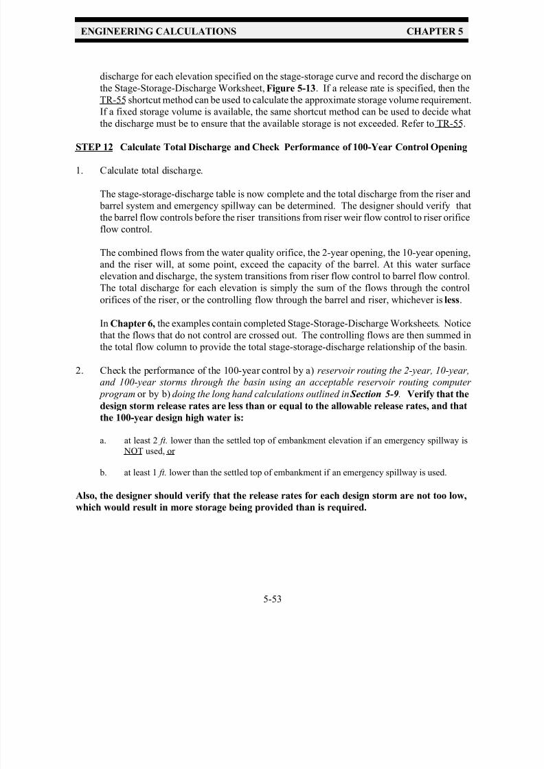
7/30/2019 Virginia Stormwater Managment Handbook Volume_II.pdf
http://slidepdf.com/reader/full/virginia-stormwater-managment-handbook-volumeiipdf 175/354
ENGINEERING CALCULATIONS CHAPTER 5
5-53
discharge for each elevation specified on the stage-storage curve and record the discharge on
the Stage-Storage-Discharge Worksheet, Figure 5-13. If a release rate is specified, then the
TR-55 shortcut method can be used to calculate the approximate storage volume requirement.
If a fixed storage volume is available, the same shortcut method can be used to decide what
the discharge must be to ensure that the available storage is not exceeded. Refer to TR-55.
STEP 12 Calculate Total Discharge and Check Performance of 100-Year Control Opening
1. Calculate total discharge.
The stage-storage-discharge table is now complete and the total discharge from the riser and
barrel system and emergency spillway can be determined. The designer should verify that
the barrel flow controls before the riser transitions from riser weir flow control to riser orifice
flow control.
The combined flows from the water quality orifice, the 2-year opening, the 10-year opening,and the riser will, at some point, exceed the capacity of the barrel. At this water surface
elevation and discharge, the system transitions from riser flow control to barrel flow control.
The total discharge for each elevation is simply the sum of the flows through the control
orifices of the riser, or the controlling flow through the barrel and riser, whichever is less.
In Chapter 6, the examples contain completed Stage-Storage-Discharge Worksheets. Notice
that the flows that do not control are crossed out. The controlling flows are then summed in
the total flow column to provide the total stage-storage-discharge relationship of the basin.
2. Check the performance of the 100-year control by a) reservoir routing the 2-year, 10-year,
and 100-year storms through the basin using an acceptable reservoir routing computer program or by b) doing the long hand calculations outlined in Section 5-9. Verify that the
design storm release rates are less than or equal to the allowable release rates, and that
the 100-year design high water is:
a. at least 2 ft. lower than the settled top of embankment elevation if an emergency spillway is
NOT used, or
b. at least 1 ft. lower than the settled top of embankment if an emergency spillway is used.
Also, the designer should verify that the release rates for each design storm are not too low,
which would result in more storage being provided than is required.

7/30/2019 Virginia Stormwater Managment Handbook Volume_II.pdf
http://slidepdf.com/reader/full/virginia-stormwater-managment-handbook-volumeiipdf 176/354
ENGINEERING CALCULATIONS CHAPTER 5
5-54
FIGURE 5 - 13
Stage - Storage - Discharge Worksheet, Example 1

7/30/2019 Virginia Stormwater Managment Handbook Volume_II.pdf
http://slidepdf.com/reader/full/virginia-stormwater-managment-handbook-volumeiipdf 177/354
ENGINEERING CALCULATIONS CHAPTER 5
5-55
FIGURE 5 - 14
Typical Hydraulic Head Values - Multi-Stage Riser
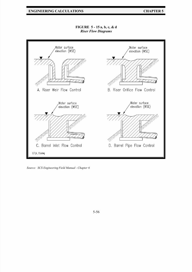
7/30/2019 Virginia Stormwater Managment Handbook Volume_II.pdf
http://slidepdf.com/reader/full/virginia-stormwater-managment-handbook-volumeiipdf 178/354
ENGINEERING CALCULATIONS CHAPTER 5
5-56
FIGURE 5 - 15 a, b, c, & d
Riser Flow Diagrams
Source: SCS Engineering Field Manual - Chapter 6
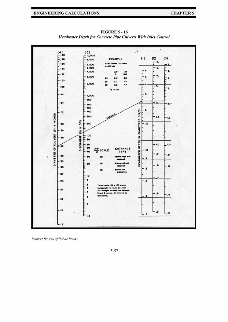
7/30/2019 Virginia Stormwater Managment Handbook Volume_II.pdf
http://slidepdf.com/reader/full/virginia-stormwater-managment-handbook-volumeiipdf 179/354
ENGINEERING CALCULATIONS CHAPTER 5
5-57
FIGURE 5 - 16
Headwater Depth for Concrete Pipe Culverts With Inlet Control
Source: Bureau of Public Roads

7/30/2019 Virginia Stormwater Managment Handbook Volume_II.pdf
http://slidepdf.com/reader/full/virginia-stormwater-managment-handbook-volumeiipdf 180/354

7/30/2019 Virginia Stormwater Managment Handbook Volume_II.pdf
http://slidepdf.com/reader/full/virginia-stormwater-managment-handbook-volumeiipdf 181/354
ENGINEERING CALCULATIONS CHAPTER 5
5-59
Type of Structure and Design of Entrance Coefficient K e
Pipe, Concrete
Projecting from fill, socket end (groove end) . . . . . . . . . . . . . . . . . . 0.2Projecting from fill, square cut end . . . . . . . . . . . . . . . . . . . . . . . . . . 0.5
Headwall or headwall and wingwalls
Socket end of pipe (groove end) . . . . . . . . . . . . . . . . . . . . . . . 0.2
Square end . . . . . . . . . . . . . . . . . . . . . . . . . . . . . . . . . . . . . . . . 0.5
Rounded (radius = 1/12D) . . . . . . . . . . . . . . . . . . . . . . . . . . . . 0.2
Mitered to conform to fill slope . . . . . . . . . . . . . . . . . . . . . . . . . . . . . 0.7
*End-section conforming to fill slope . . . . . . . . . . . . . . . . . . . . . . . . 0.5
Pipe, or Pipe-Arch, Corrugated Metal
Projecting from fill (no headwall) . . . . . . . . . . . . . . . . . . . . . . . . . . . 0.9
Headwall or headwall and wingwallsSquare end . . . . . . . . . . . . . . . . . . . . . . . . . . . . . . . . . . . . . . . . 0.5
Mitered to conform to fill slope . . . . . . . . . . . . . . . . . . . . . . . . . . . . . 0.7
*End-section conforming to fill slope . . . . . . . . . . . . . . . . . . . . . . . . 0.5
*Note: “End-section conforming to fill slope” made of either metal or concrete, is the
section commonly available from manufacturers. Based on limited hydraulic tests, it
appears to be equivalent in operation to a headwall in either inlet or outlet control.
TABLE 5 - 9
Pipe Entrance Loss Coefficients - K e
Source - Federal Highway Administration, Bureau of Public Roads

7/30/2019 Virginia Stormwater Managment Handbook Volume_II.pdf
http://slidepdf.com/reader/full/virginia-stormwater-managment-handbook-volumeiipdf 182/354
ENGINEERING CALCULATIONS CHAPTER 5
5-60
TABLE 5 - 10
Head Loss Coefficients, K p , for Circular and Square Conduits Flowing Full

7/30/2019 Virginia Stormwater Managment Handbook Volume_II.pdf
http://slidepdf.com/reader/full/virginia-stormwater-managment-handbook-volumeiipdf 183/354
ENGINEERING CALCULATIONS CHAPTER 5
5-61
Note that this procedure is for riprap outlet protection at the
downstream end of an embankment conduit. It DOES NOT apply to
continuous rock linings of channels or streams. Refer to Figure 5 -19.
Outflows from stormwater management facilities must be discharged to an
adequate channel. Basins discharging onto a flat area with no defined channel
will usually require a channel to be provided which can convey the design flows.
STEP 13 Design Outlet Protection
With the total discharge known for the full range of design storms, adequate outlet protection can
now be designed. Protection is necessary to prevent scouring at the outlet and to help reduce the
potential for downstream erosion by reducing the velocity and energy of the concentrated discharge.The most common form of outlet protection is a riprap-lined apron, constructed at zero grade for a
specified distance, as determined by the outlet flow rate and tailwater elevation. The design
procedure follows:
1. Determine the tailwater depth, for the appropriate design storm, immediately below the
discharge pipe.
Typically, the discharge pipe from a stormwater management facility is sized to carry the allowabledischarge from the 10-year frequency design storm. Manning’s equation can be used to find thewater surface elevation in the receiving channel for the 10-year storm, which represents the tailwater elevation. If the tailwater depth is less than half the outlet pipe diameter, it is called a minimumtailwater condition. If the tailwater depth is greater than half the outlet pipe diameter, it is called amaximum tailwater condition. Stormwater basins that discharge onto flat areas with no definedchannel may be assumed to have a minimum tailwater condition.
2. Determine the required riprap size, D50, and apron length, La.
Enter the appropriate figure, either Figure 5-20: Minimum Tailwater Condition, or Figure
5-21: Maximum Tailwater Condition, with the design discharge of the pipe spillway to read the
required apron length, L s. (The apron length should not be less than 10 feet.)
3. Determine the required riprap apron width, W .
When the pipe discharges directly into a well-defined channel, the apron shall extend across the
channel bottom and up the channel banks to an elevation 1 foot above the maximum tailwater depth
or the top of bank, whichever is less.
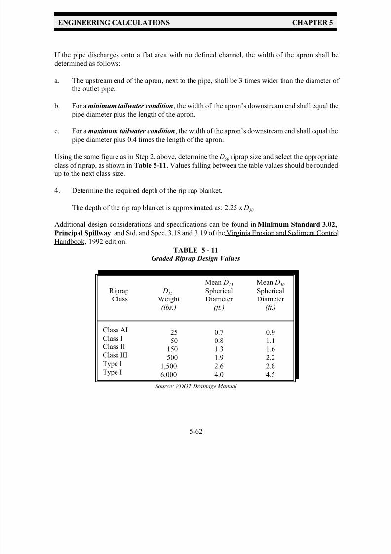
7/30/2019 Virginia Stormwater Managment Handbook Volume_II.pdf
http://slidepdf.com/reader/full/virginia-stormwater-managment-handbook-volumeiipdf 184/354
ENGINEERING CALCULATIONS CHAPTER 5
5-62
If the pipe discharges onto a flat area with no defined channel, the width of the apron shall be
determined as follows:
a. The upstream end of the apron, next to the pipe, shall be 3 times wider than the diameter of
the outlet pipe.
b. For a minimum tailwater condition, the width of the apron’s downstream end shall equal the
pipe diameter plus the length of the apron.
c. For a maximum tailwater condition, the width of the apron’s downstream end shall equal the
pipe diameter plus 0.4 times the length of the apron.
Using the same figure as in Step 2, above, determine the D50 riprap size and select the appropriate
class of riprap, as shown in Table 5-11. Values falling between the table values should be rounded
up to the next class size.
4. Determine the required depth of the rip rap blanket.
The depth of the rip rap blanket is approximated as: 2.25 x D50
Additional design considerations and specifications can be found in Minimum Standard 3.02,
Principal Spillway and Std. and Spec. 3.18 and 3.19 of the Virginia Erosion and Sediment Control
Handbook, 1992 edition.
TABLE 5 - 11
Graded Riprap Design Values
Riprap
Class
D15
Weight
(lbs.)
Mean D15
Spherical
Diameter
(ft.)
Mean D50
Spherical
Diameter
(ft.)
Class AI
Class I
Class II
Class III
Type I
Type I
25
50
150
500
1,5006,000
0.7
0.8
1.3
1.9
2.64.0
0.9
1.1
1.6
2.2
2.84.5
Source: VDOT Drainage Manual

7/30/2019 Virginia Stormwater Managment Handbook Volume_II.pdf
http://slidepdf.com/reader/full/virginia-stormwater-managment-handbook-volumeiipdf 185/354
ENGINEERING CALCULATIONS CHAPTER 5
5-63
FIGURE 5 - 19
Outlet Protection Detail
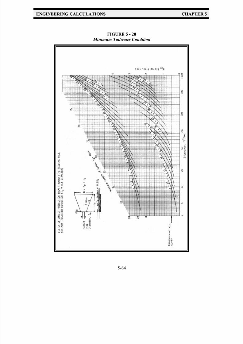
7/30/2019 Virginia Stormwater Managment Handbook Volume_II.pdf
http://slidepdf.com/reader/full/virginia-stormwater-managment-handbook-volumeiipdf 186/354
ENGINEERING CALCULATIONS CHAPTER 5
5-64
FIGURE 5 - 20
Minimum Tailwater Condition
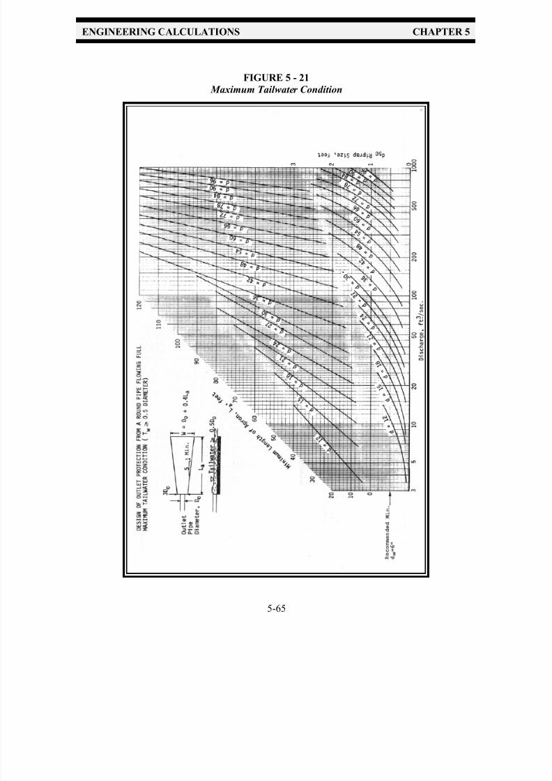
7/30/2019 Virginia Stormwater Managment Handbook Volume_II.pdf
http://slidepdf.com/reader/full/virginia-stormwater-managment-handbook-volumeiipdf 187/354
ENGINEERING CALCULATIONS CHAPTER 5
5-65
FIGURE 5 - 21
Maximum Tailwater Condition

7/30/2019 Virginia Stormwater Managment Handbook Volume_II.pdf
http://slidepdf.com/reader/full/virginia-stormwater-managment-handbook-volumeiipdf 188/354
ENGINEERING CALCULATIONS CHAPTER 5
5-66
STEP 14 Perform Buoyancy Calculation
The design of a multi-stage riser structure must include a buoyancy analysis for the riser and footing.
When the ground is saturated and ponded runoff is at an elevation higher than the footing of the riser
structure, the riser structure acts like a vessel. During this time, the riser is subject to uplifting, buoyant forces that are relative in strength to the volume of water displaced. Flotation will occur
when the weight of the structure is less than or equal to the buoyant force exerted by the
water. Flotation forces on the riser can lead to failure of the connection between the riser structure
and barrel, and any other rigid connections. Eventually, this can also lead to the failure of the
embankment.
A buoyancy calculation is the summation of all forces acting on the riser. The upward force is the
weight of the water, or 62.4 lb/ft 3. The downward force includes the weight of the riser structure, any
components, such as trash racks, and the weight of the soil above the footing. Note that conventional
reinforced concrete weighs about 150 lb/ft 3 and the unit weight of soil is approximately 120 lb/ft 3 .
The weight of components such as trash racks, anti-vortex devices, hoods, etc. is very specific toeach structure and, depending upon the design, may or may not be significant in comparison to the
other forces. If an extended base footing is used below the ground surface to support the control
structure, then the weight of the soil above the footing may also be a significant force.
The outlet pipe is excluded from the buoyancy analysis for the control structure. However, the barrel
should be analyzed separately to insure that it is not subject to flotation. The method used to attach
the control structure to the outlet pipe is considered to have no bearing on the potential for these
components to float.
The following procedure compares the upward force (buoyant force) to the downward force
(structure weight). To maintain adequate stability, the downward force should be a minimum of 1.25 times the upward force.
1. Determine the buoyant force.
The buoyant force is the total volume of the riser structure and base, using outside dimensions (i.e.,
the total volume displacement of the riser structure) multiplied by the unit weight of water (62.4
lb/ft 3).
2. Determine the downward or resisting force.
The downward force is the total volume of the riser walls below the crest, including any top slab,footing, etc., less the openings for any pipe connections, multiplied by the unit weight of reinforced
concrete (150 lb/ft 3). Additional downward forces from any components may also be added,
including the weight of the soil above the extended footing.
3. Decide if the downward force is greater than the buoyant force by a factor of 1.25 or more.

7/30/2019 Virginia Stormwater Managment Handbook Volume_II.pdf
http://slidepdf.com/reader/full/virginia-stormwater-managment-handbook-volumeiipdf 189/354
ENGINEERING CALCULATIONS CHAPTER 5
5-67
If the downward force is not greater than the buoyant force by a factor of 1.25 or more, then
additional weight must be added to the structure. This can be done by sinking the riser footing
deeper into the ground and adding concrete to the base. Note that this will also increase the buoyant
force, but since the unit weight of concrete is more than twice that of water, the net result will be anincrease in the downward force. The downward and buoyant forces should be adjusted accordingly,
and step 3 repeated.
STEP 15 Provide Seepage Control
Seepage control should be provided for the pipe through the embankment. The two most common
devices for controlling seepage are 1) filter and drainage diaphragms and 2) anti-seep collars. The
use of these devices is discussed in detail in Minimum Standard 3.02, Principal Spillway. Note that
filter and drainage diaphragms are preferred over anti-seep collars for controlling seepage along pipe
conduits.
a. Filter & Drainage Diaphragms
The design of filter and drainage diaphragms depends on the foundation and embankment soils and is outside
the scope of this manual. When filter and drainage diaphragms are warranted, their design and construction
should be supervised by a registered professional engineer. Design criteria and construction procedures for
filter and drainage diaphragms can be found in the following references:
• USDA SCS TR-60
• USDA SCS Soil Mechanics Note No. 1: Guide for Determining the Gradation of Sand
and Gravel Filters*
• USDA SCS Soil Mechanics Note No. 3: Soil Mechanics Consideration for Embankment Drains*
• U.S. Department of the Interior ACER Technical Memorandum No. 9: Guidelines for
Controlling Seepage Along Conduits Through Embankments
* These publications include design procedures and examples and are provided in Appendix 5B.
b. Anti-Seep Collars
The Bureau of Reclamation, the U.S. Army Corps of Engineers and the Soil Conservation Service
no longer recommend the use of anti-seep collars. In 1987, the Bureau of Reclamation issuedTechnical Memorandum No. 9 that states:
“When a conduit is selected for a waterway through an earth or rockfill embankment,
cutoff [anti-seep]collars will not be selected as the seepage control measure.”
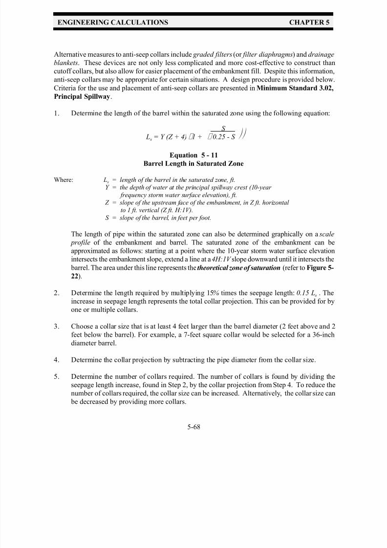
7/30/2019 Virginia Stormwater Managment Handbook Volume_II.pdf
http://slidepdf.com/reader/full/virginia-stormwater-managment-handbook-volumeiipdf 190/354
ENGINEERING CALCULATIONS CHAPTER 5
5-68
S
L s = Y (Z + 4) ˆ 1 + ˆ 0.25 - S
Alternative measures to anti-seep collars include graded filters (or filter diaphragms) and drainage
blankets. These devices are not only less complicated and more cost-effective to construct than
cutoff collars, but also allow for easier placement of the embankment fill. Despite this information,
anti-seep collars may be appropriate for certain situations. A design procedure is provided below.
Criteria for the use and placement of anti-seep collars are presented in Minimum Standard 3.02,Principal Spillway.
1. Determine the length of the barrel within the saturated zone using the following equation:
Equation 5 - 11
Barrel Length in Saturated Zone
Where: L s = length of the barrel in the saturated zone, ft.Y = the depth of water at the principal spillway crest (10-year
frequency storm water surface elevation), ft.
Z = slope of the upstream face of the embankment, in Z ft. horizontal
to 1 ft. vertical (Z ft. H:1V).
S = slope of the barrel, in feet per foot.
The length of pipe within the saturated zone can also be determined graphically on a scale
profile of the embankment and barrel. The saturated zone of the embankment can be
approximated as follows: starting at a point where the 10-year storm water surface elevation
intersects the embankment slope, extend a line at a 4H:1V slope downward until it intersects the
barrel. The area under this line represents the theoretical zone of saturation (refer to Figure 5-
22).
2. Determine the length required by multiplying 15% times the seepage length: 0.15 L s . The
increase in seepage length represents the total collar projection. This can be provided for by
one or multiple collars.
3. Choose a collar size that is at least 4 feet larger than the barrel diameter (2 feet above and 2
feet below the barrel). For example, a 7-feet square collar would be selected for a 36-inch
diameter barrel.
4. Determine the collar projection by subtracting the pipe diameter from the collar size.
5. Determine the number of collars required. The number of collars is found by dividing the
seepage length increase, found in Step 2, by the collar projection from Step 4. To reduce the
number of collars required, the collar size can be increased. Alternatively, the collar size can
be decreased by providing more collars.

7/30/2019 Virginia Stormwater Managment Handbook Volume_II.pdf
http://slidepdf.com/reader/full/virginia-stormwater-managment-handbook-volumeiipdf 191/354
ENGINEERING CALCULATIONS CHAPTER 5
5-69
FIGURE 5 - 22
Phreatic Line Graphical Determination
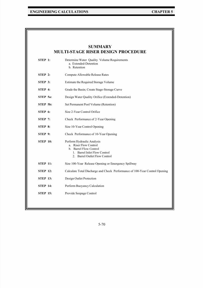
7/30/2019 Virginia Stormwater Managment Handbook Volume_II.pdf
http://slidepdf.com/reader/full/virginia-stormwater-managment-handbook-volumeiipdf 192/354
ENGINEERING CALCULATIONS CHAPTER 5
5-70
SUMMARYMULTI-STAGE RISER DESIGN PROCEDURE
STEP 1: Determine Water Quality Volume Requirements
a. Extended-Detention
b. Retention
STEP 2: Compute Allowable Release Rates
STEP 3: Estimate the Required Storage Volume
STEP 4: Grade the Basin; Create Stage-Storage Curve
STEP 5a: Design Water Quality Orifice (Extended-Detention)
STEP 5b: Set Permanent Pool Volume (Retention)
STEP 6: Size 2-Year Control Orifice
STEP 7: Check Performance of 2-Year Opening
STEP 8: Size 10-Year Control Opening
STEP 9: Check Performance of 10-Year Opening
STEP 10: Perform Hydraulic Analysis
a. Riser Flow Control b. Barrel Flow Control
1. Barrel Inlet Flow Control
2. Barrel Outlet Flow Control
STEP 11: Size 100-Year Release Opening or Emergency Spillway
STEP 12: Calculate Total Discharge and Check Performance of 100-Year Control Opening
STEP 13: Design Outlet Protection
STEP 14: Perform Buoyancy Calculation
STEP 15: Provide Seepage Control

7/30/2019 Virginia Stormwater Managment Handbook Volume_II.pdf
http://slidepdf.com/reader/full/virginia-stormwater-managment-handbook-volumeiipdf 193/354
ENGINEERING CALCULATIONS CHAPTER 5
5-71
The design maximum water surface elevations for the emergency spillway should
be at least 1 foot lower than the settled top of the embankment. Refer to Minimum
Standard 3.03, Vegetated Emergency Spillways.
Procedure 1:
5-8 EMERGENCY SPILLWAY DESIGN
A vegetated emergency spillway is designed to convey a predetermined design flood volume without
excessive velocities and without overtopping the embankment.
Two design methods are presented here. The first (Procedure 1) is a conservative design procedure
which is also found in The Virginia Erosion & Sediment Control Handbook, 1992 edition, Std. &
Spec. 3.14. This procedure is typically acceptable for stormwater management basins. The second
method (Procedure 2) utilizes the roughness, or retardance, and durability of the vegetation and soils
within the vegetated spillway. This second design is appropriate for larger or regional stormwater
facilities where construction inspection and permanent maintenance are more readily enforced.
These larger facilities typically control relatively large watersheds and are located such that the
stability of the emergency spillway is essential to safeguard downstream features.
The following design procedures establish a stage-discharge relationship ( H p versus Q) for a
vegetated emergency spillway serving a stormwater management basin (refer to Figure 5-23).
The information required for these designs includes the determination of the hydrology for the
watershed draining to the basin. Any of the methods, as outlined in Chapter 4, may be used. The
design should include calculations for the allowable release rate from the basin if the spillway is to
be used to control a design frequency storm. Otherwise, the design peak flow rate should be
calculated based on the spillway design flood, or downstream conditions.
(In general, a vegetated emergency spillway should not be used as an outlet for any storm less than
the 100-year frequency storm, unless it is armored with a non-erodible material. The designer must
consider the depth of the riprap blanket when riprap is used to armor the spillway. As noted
previously, Class I riprap would require a blanket thickness or stone depth of 30" which may addconsiderable height to the embankment.)
1. Determine the design peak rate of inflow from the spillway design flood into the basin using
the developed condition hydrology or determine the allowable design peak release rate, Q,
from the basin based on downstream conditions or watershed requirements.
2. Estimate the maximum water surface elevation and calculate the maximum flow through the
7/30/2019 Virginia Stormwater Managment Handbook Volume_II.pdf
http://slidepdf.com/reader/full/virginia-stormwater-managment-handbook-volumeiipdf 194/354
7/30/2019 Virginia Stormwater Managment Handbook Volume_II.pdf
http://slidepdf.com/reader/full/virginia-stormwater-managment-handbook-volumeiipdf 195/354
ENGINEERING CALCULATIONS CHAPTER 5
5-73
Procedure 2:
Q(cfs)
q(cfs/ft)' ft.
is less than the 4% provided, and the length of exit channel is required to be 63 ft . The velocity
within the exit channel is 4.7 ft/s at an exit channel slope of 2.7%. Since the provided exit
channel slope is 4.0%, erosive velocities may warrant special treatment of the exit channel.
5. Add the elevation corresponding to 1.3 ft . above the crest of the emergency spillway to theStage-Storage-Discharge Worksheet.
1. Determine the design peak rate of inflow from the spillway design flood into the basin, using
the developed condition hydrology, or determine the allowable design peak release rate , Q,
from the basin based on downstream conditions or watershed requirements.
2. Estimate the maximum water surface elevation and calculate the associated flow through the
riser and barrel system for this elevation. Subtract this flow value from the design peak rateof inflow to determine the desired maximum spillway design discharge.
3. Position the emergency spillway on the basin grading plan at an embankment abutment.
4. Determine the slope, so , of the proposed exit channel, and the length, L, and elevation of the
proposed level section from the basin grading plan.
5. Classify the natural soils around the spillway as erosion resistant or easily erodible soils.
6. Determine the type and height of vegetative cover to be used to stabilize the spillway.
7. Determine the permissible velocity, v, from Table 3-03.1, based on the vegetative cover, soil
classification, and the slope of the exit channel, so .
8. Determine the retardance classification of the spillway based on the type and height of
vegetative cover from Table 3-03.2.
9. Determine the unit discharge of the spillway, q, in cfs/ft , from Table 5-13(a-d) for the selected
retardance, the maximum permissible velocity, v, and the slope of the exit channel, so .
10. Determine the required bottom width of the spillway, in ft., by dividing the allowable or design
discharge, Q , by the spillway unit discharge, q:
11. Determine the depth of flow, H p , upstream of the control section based on the length of the

7/30/2019 Virginia Stormwater Managment Handbook Volume_II.pdf
http://slidepdf.com/reader/full/virginia-stormwater-managment-handbook-volumeiipdf 196/354
ENGINEERING CALCULATIONS CHAPTER 5
5-74
level section, L, from Table 5-13(a-d).
12. Enter the stage-discharge information into the stage-storage-discharge table.
The following examples use Tables 3-03.1, 3-03.2 and 5-13 to find the capacity of a vegetatedemergency spillway.
Example Procedure 2:
Given: Q = 250 cfs (determined from post-developed condition hydrology)
so = 4% (slope of exit channel)
L = 50 ft .(length of level section)
Erosion resistant soils
Sod forming grass-legume mixture cover, 6 to 10-inch height
Find: Permissible velocity, v, width of spillway, b, depth of water above the spillway crest, H p.
Solution: Complete Steps 1 through 12 of design Procedure 2 for vegetated emergency spillways by using
the given information as follows:
1. Peak rate of inflow: given Q = 250 cfs.
2. The flow through the riser and barrel at the estimated maximum water surface elevation is
calculated to be 163 cfs. The desired maximum spillway design discharge is 250 cfs - 163 cfs
= 87 cfs.
3. Emergency spillway excavated into undisturbed material.
4. Slope of exit channel, and length and elevation of level section: given, so = 4%, L = 50 ft.,
elevation = 100.0 feet (given).
5. Soil classification: given, erosion resistant soils.
6. Vegetative cover: given, sod-forming grass-legume mixture.
7. Permissible velocity v = 5 ft/s from Table 3-03.1 for sod-forming grass-legume mixtures,
erosion resistant soils, and exit channel slope so = 4%.
8. Retardance classification, C , from Table 3.03.2 for sod-forming grass-legume mixtures,expected height = 6 to 10 inches.
9. The unit discharge of the spillway q = 3 cfs/ft from Table 5-13c for Retardance C , maximum
permissible velocity v = 5 ft/s, and exit channel slope so = 4%.
7/30/2019 Virginia Stormwater Managment Handbook Volume_II.pdf
http://slidepdf.com/reader/full/virginia-stormwater-managment-handbook-volumeiipdf 197/354
ENGINEERING CALCULATIONS CHAPTER 5
5-75
10. The required bottom width b = Q q = 87 cfs/ 3 cfs/ft = 29 ft .
11. The depth of flow, H p, from Table 5-13c for Retardance C ; enter at q = 3 cfs/ft , find H p = 1.4
ft. for level section L = 50 ft.
12. The stage-discharge relationship: at stage elevation 1.4 feet above the spillway crest (101.4' ),
the discharge is 87 cfs.
Example Procedure 2:
Given: Q = 175 cfs (determined from post-developed hydrology)
so = 8 % (slope of exit channel)
L = 25 ft . (length of level section)
Easily erodible soil
Bahiagrass, good stand, 11 to 24 inches expected
Find: Permissible velocity, v, width of spillway, b, depth of water above the spillway crest, H p.Analyze the spillway for stability during the vegetation establishment period, and capacity once
adequate vegetation is achieved.
Solution: Complete Steps 1 through 12 of the design Procedure 2 for vegetated emergency spillways by
using the given information as follows:
1. Q = 175 cfs.
2. The flow through the riser and barrel at the estimated maximum water surface elevation is
calculated to be 75 cfs. The desired maximum spillway design discharge is 175 cfs - 75 cfs =
100 cfs.
3. Emergency spillway in undisturbed ground.
4. so = 8 %; L = 25 ft ., elevation = 418.0 feet (given)
5. Easily erodible soils.
6. Bahiagrass, good stand, 11 to 24 inches expected.
7. Permissable velocity, v = 5 ft/s, from Table 3-03.1.
8. a) Retardance used for stability during the establishment period - good stand of vegetation
2 to 6 inches; Retardance D.
b) Retardance used for capacity - good stand of vegetation 11 to 24 inches; Retardance B.

7/30/2019 Virginia Stormwater Managment Handbook Volume_II.pdf
http://slidepdf.com/reader/full/virginia-stormwater-managment-handbook-volumeiipdf 198/354
ENGINEERING CALCULATIONS CHAPTER 5
5-76
9. Unit discharge q = 2 cfs/ft for stability. From Table 5-13d for Retardance D, permissable
velocity, v = 5 ft/s., and so = 8%
10. Bottom width b = Q/ q = 100 cfs/ 2 cfs/ ft = 50 ft. (stability)
11. The depth of flow , H p, for capacity. From Table 5-13b for Retardance B, enter at
q = 2 cfs/ft , find H p = 1.4 ft. for L = 25 ft .
12. The stage-discharge relationship: at stage (elevation) 1.4 ft. above the spillway crest (419.4' ),
the discharge, Q, is 100 cfs.

7/30/2019 Virginia Stormwater Managment Handbook Volume_II.pdf
http://slidepdf.com/reader/full/virginia-stormwater-managment-handbook-volumeiipdf 199/354
ENGINEERING CALCULATIONS CHAPTER 5
5-77
TABLE 5-12
Design Data for Earth Spillways
Source: USDA - SCS

7/30/2019 Virginia Stormwater Managment Handbook Volume_II.pdf
http://slidepdf.com/reader/full/virginia-stormwater-managment-handbook-volumeiipdf 200/354
ENGINEERING CALCULATIONS CHAPTER 5
5-78
TABLE 5 - 13a
H p and Slope Range for Discharge, Velocity and Crest Length - Retardance A
Max. Velocity, v
( ft/s)
Unit Discharge, q
(cfs/ft )
Depth of Water Above
Spillway Crest, H p ( ft.)
Length of Level Section, L
(ft.)
Slope Range, so
%
Min. Max.
25 50 100 200
3
4
4
5
67
8
3
4
5
6
710
12.5
2.3
2.3
2.5
2.6
2.73.0
3.3
2.5
2.5
2.6
2.7
2.83.2
3.5
2.7
2.8
2.9
3.0
3.13.4
3.7
3.1
3.1
3.2
3.3
3.53.8
4.1
1
1
1
1
11
1
11
12
7
9
129
10
Source: SCS Engineering Field Manual
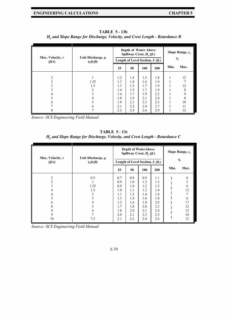
7/30/2019 Virginia Stormwater Managment Handbook Volume_II.pdf
http://slidepdf.com/reader/full/virginia-stormwater-managment-handbook-volumeiipdf 201/354
ENGINEERING CALCULATIONS CHAPTER 5
5-79
TABLE 5 - 13b
H p and Slope Range for Discharge, Velocity, and Crest Length - Retardance B
Max. Velocity, v
( ft/s)
Unit Discharge, q
(cfs/ft )
Depth of Water Above
Spillway Crest, H p ( ft.)
Length of Level Section, L (ft.)
Slope Range, so
%
Min. Max.25 50 100 200
2
2
3
3
4
5
6
78
1
1.25
1.5
2
3
4
5
67
1.2
1.3
1.3
1.4
1.6
1.8
1.9
2.12.2
1.4
1.4
1.5
1.5
1.7
1.9
2.1
2.22.4
1.5
1.6
1.7
1.7
1.9
2.1
2.3
2.42.6
1.8
1.9
1.9
1.9
2.2
2.4
2.5
2.72.9
1 12
1 7
1 12
1 8
1 9
1 8
1 10
1 111 12
Source: SCS Engineering Field Manual
TABLE 5 - 13c
H p and Slope Range for Discharge, Velocity, and Crest Length - Retardance C
Max. Velocity, v
( ft/s)
Unit Discharge, q
(cfs/ft )
Depth of WaterAbove
Spillway Crest, H p ( ft.)
Length of Level Section, L (ft.)
Slope Range, so
%
Min. Max.25 50 100 200
2
2
3
4
4
5
6
8
9
910
0.5
1
1.25
1.5
2
3
4
5
6
77.5
0.7
0.9
0.9
1.0
1.1
1.3
1.5
1.7
1.8
2.02.1
0.8
1.0
1.0
1.1
1.2
1.4
1.6
1.8
2.0
2.12.2
0.9
1.2
1.2
1.2
1.4
1.6
1.8
2.0
2.1
2.32.4
1.1
1.3
1.3
1.4
1.6
1.8
2.0
2.2
2.4
2.52.6
1
1
1
1
1
1
1
11
6
3
6
12
7
6
12
12
12
1012
Source: SCS Engineering Field Manual

7/30/2019 Virginia Stormwater Managment Handbook Volume_II.pdf
http://slidepdf.com/reader/full/virginia-stormwater-managment-handbook-volumeiipdf 202/354
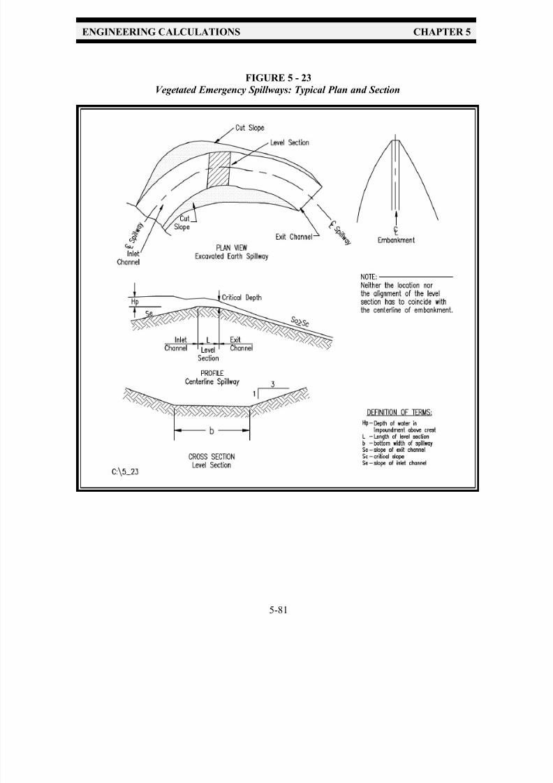
7/30/2019 Virginia Stormwater Managment Handbook Volume_II.pdf
http://slidepdf.com/reader/full/virginia-stormwater-managment-handbook-volumeiipdf 203/354
ENGINEERING CALCULATIONS CHAPTER 5
5-81
FIGURE 5 - 23
Vegetated Emergency Spillways: Typical Plan and Section

7/30/2019 Virginia Stormwater Managment Handbook Volume_II.pdf
http://slidepdf.com/reader/full/virginia-stormwater-managment-handbook-volumeiipdf 204/354
ENGINEERING CALCULATIONS CHAPTER 5
5-82
Procedure:
5-9 HYDROGRAPH ROUTING
This section presents the methodology for routing a runoff hydrograph through an existing or
proposed stormwater basin. The "level pool" or storage indication routing technique is one of the
simplest and most commonly used methods, and is based on the continuity equation:
I - O = ds / dt
Inflow - Outflow = Change in Storage over time
The goal of the routing process is to create an outflow hydrograph that is the result of the combined
effects of the outlet device and the available storage. This will allow the designer to evaluate the
performance of the outlet device or the basin storage volume, or both. When multiple iterations are
required to create the most efficient basin shape, the routing procedure can be time consuming and
cumbersome, especially when done by hand using the methods presented in this section. It should
be noted that several computer programs are available to help complete the routing procedure.
A step-by-step procedure for routing a runoff hydrograph through a stormwater basin is given below.
Note that the first four steps are part of the multi-stage riser design of the previous section. Due to
the complexity of this procedure, Example 1 from Chapter 6 will be used. Note that the water
quality volume is not considered and only one design storm will be routed, the 2-year storm. Other
design frequency storms can be easily analyzed with the same procedure. Blank worksheets for this
procedure are provided in Appendix 5D.
1. Generate a post-developed condition inflow hydrograph. The runoff hydrograph for the 2-year
frequency storm, post-developed condition from Example 1, as calculated by the SCS TR-20
computer program and shown in Figure 5-1, will be used for the inflow hydrograph. (Refer
to Chapter 6 for details on the hydrology from Example 1. Refer to Chapter 4 for
information on the hydrologic methods used.)
2. Develop the stage-storage relationship for the proposed basin. The hydrologic calculations and
the hydrograph analysis for Example 1, in Section 5-3 and Section 5-4.1, revealed that the
storage volume required to reduce the 2-year, post-developed peak discharge back to the pre-
developed rate was 35,820 ft 3. Therefore, a preliminary grading plan should have a stormwater
basin with this required storage volume, as a minimum, to control the 2-year frequency storm.The stage-storage relationship of the proposed stormwater facility can be generated by
following the procedures outlined in Section 5-5. Figure 5-10 shows the completed Storage
Volume Calculations Worksheet, and Figure 5-11 shows the stage vs. storage curve.
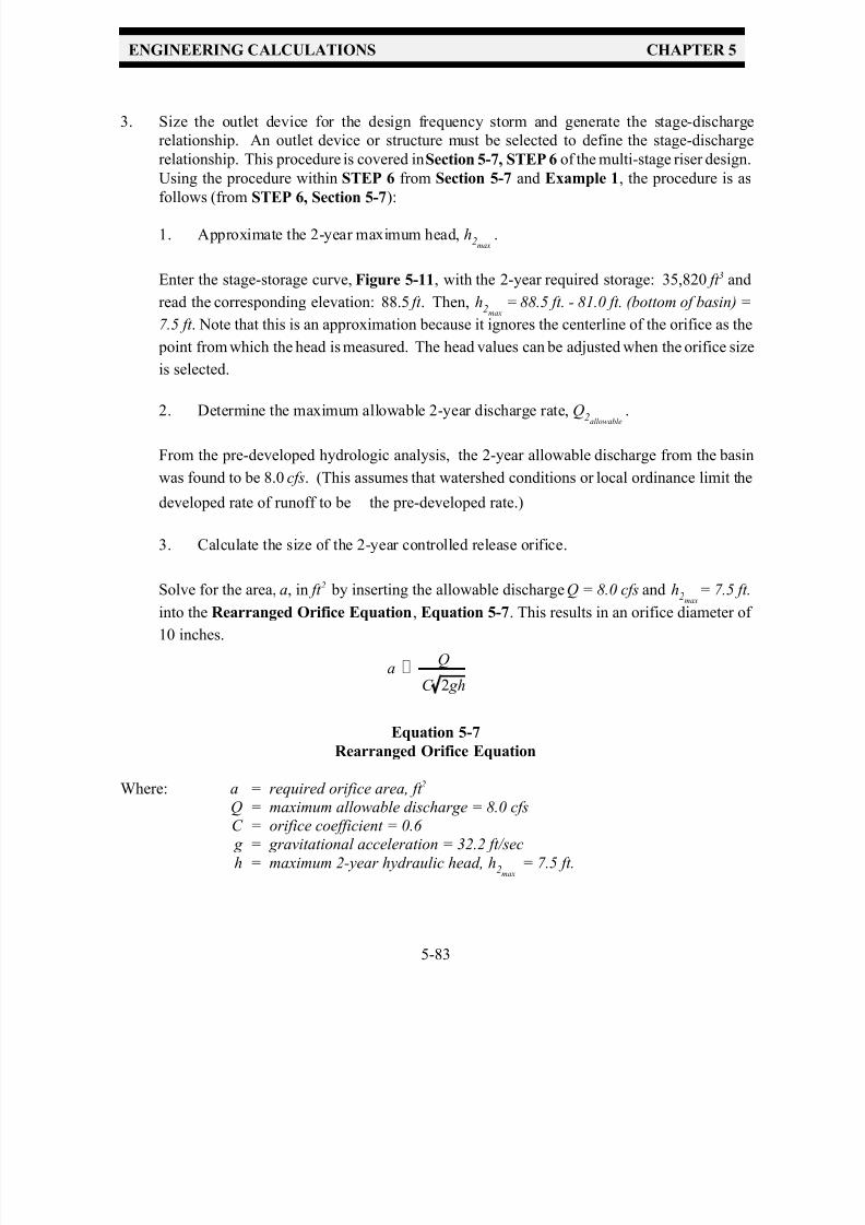
7/30/2019 Virginia Stormwater Managment Handbook Volume_II.pdf
http://slidepdf.com/reader/full/virginia-stormwater-managment-handbook-volumeiipdf 205/354
ENGINEERING CALCULATIONS CHAPTER 5
5-83
a 'Q
C 2 gh
3. Size the outlet device for the design frequency storm and generate the stage-discharge
relationship. An outlet device or structure must be selected to define the stage-discharge
relationship. This procedure is covered in Section 5-7, STEP 6 of the multi-stage riser design.
Using the procedure within STEP 6 from Section 5-7 and Example 1, the procedure is as
follows (from STEP 6, Section 5-7):
1. Approximate the 2-year maximum head, .h2max
Enter the stage-storage curve, Figure 5-11, with the 2-year required storage: 35,820 ft 3 and
read the corresponding elevation: 88.5 ft . Then, = 88.5 ft. - 81.0 ft. (bottom of basin) =h2max
7.5 ft . Note that this is an approximation because it ignores the centerline of the orifice as the
point from which the head is measured. The head values can be adjusted when the orifice size
is selected.
2. Determine the maximum allowable 2-year discharge rate, .Q2allowable
From the pre-developed hydrologic analysis, the 2-year allowable discharge from the basin
was found to be 8.0 cfs. (This assumes that watershed conditions or local ordinance limit the
developed rate of runoff to be the pre-developed rate.)
3. Calculate the size of the 2-year controlled release orifice.
Solve for the area, a, in ft 2 by inserting the allowable discharge Q = 8.0 cfs and = 7.5 ft.h2max
into the Rearranged Orifice Equation, Equation 5-7. This results in an orifice diameter of 10 inches.
Equation 5-7
Rearranged Orifice Equation
Where: a = required orifice area, ft 2
Q = maximum allowable discharge = 8.0 cfs
C = orifice coefficient = 0.6
g = gravitational acceleration = 32.2 ft/sec
h = maximum 2-year hydraulic head, = 7.5 ft.h2max
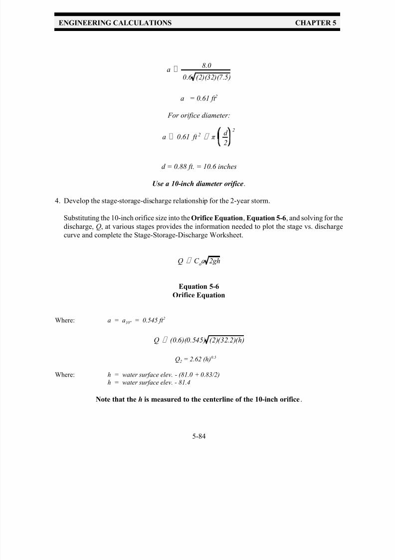
7/30/2019 Virginia Stormwater Managment Handbook Volume_II.pdf
http://slidepdf.com/reader/full/virginia-stormwater-managment-handbook-volumeiipdf 206/354

7/30/2019 Virginia Stormwater Managment Handbook Volume_II.pdf
http://slidepdf.com/reader/full/virginia-stormwater-managment-handbook-volumeiipdf 207/354
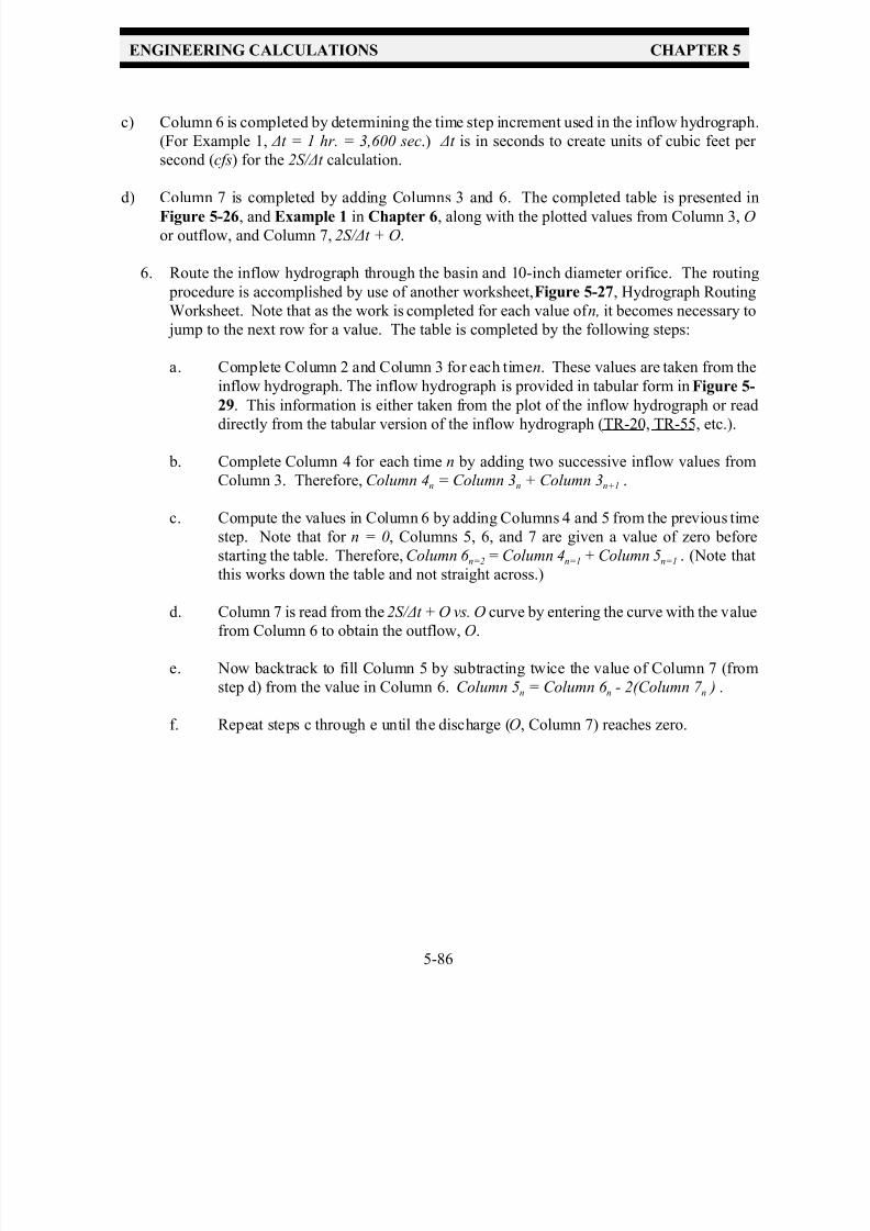
7/30/2019 Virginia Stormwater Managment Handbook Volume_II.pdf
http://slidepdf.com/reader/full/virginia-stormwater-managment-handbook-volumeiipdf 208/354

7/30/2019 Virginia Stormwater Managment Handbook Volume_II.pdf
http://slidepdf.com/reader/full/virginia-stormwater-managment-handbook-volumeiipdf 209/354
ENGINEERING CALCULATIONS CHAPTER 5
5-87
FIGURE 5 - 24
Stage vs. Discharge Curve, Example 1

7/30/2019 Virginia Stormwater Managment Handbook Volume_II.pdf
http://slidepdf.com/reader/full/virginia-stormwater-managment-handbook-volumeiipdf 210/354
ENGINEERING CALCULATIONS CHAPTER 5
5-88
FIGURE 5 - 25
Storage Indication Hydrograph Routing (2S/ ∆t + O) vs. O Worksheet
1 2 3 4 5 6 7
elevation
(ft)
stage
(ft)
outflow
(cfs)
storage
(cf)
2S
(cf)
2S/ ∆t
(cfs)
2S/ ∆t + O
(cfs)
from
planelevn - elevo
based on
outflow device
& stage
based on
stage2 × Col 4
Col 5 / ∆t of
hydrographCol 3 + Col 6

7/30/2019 Virginia Stormwater Managment Handbook Volume_II.pdf
http://slidepdf.com/reader/full/virginia-stormwater-managment-handbook-volumeiipdf 211/354

7/30/2019 Virginia Stormwater Managment Handbook Volume_II.pdf
http://slidepdf.com/reader/full/virginia-stormwater-managment-handbook-volumeiipdf 212/354
ENGINEERING CALCULATIONS CHAPTER 5
5-90
n = 1
FIGURE 5 - 27
Storage Indication Hydrograph Routing Worksheet
1 2 3 4 5 6 7
n Time
(min)
I n(cfs)
I n + I n+1
(cfs)
2S n / ∆t - On
(cfs)
2S n+1 / ∆t + On+1
(cfs)
On+1
(cfs)
from
hydrograph
Col 3n +Col 3n+1 Col 6 n - 2(Col 7 n ) Col 4n-1 + Col 5n-1 from chart;
use Col 6 n
0 0 0 0
The above steps are repeated here for the first four time steps in Example 1 and displayed in the
completed Hydrograph Routing Worksheet, Figure 5-28.
1. Columns 2 and 3 are completed for each time step using the inflow hydrograph.
2. Column 4 is completed as follows:
Column 4n = Column 3n + Column 3n+1
for n = 1: Column 4n=1 = Column 3n=1 + Column 3n=2
Column 4n=1 = 0 + 0.32 = 0.32
for n = 2: Column 4n=2 = 0.3 + 23.9 = 24.2
for n = 3: Column 4n=3 = 23.9 + 4.6 = 28.5
for n = 4: Column 4n=4 = 4.6 + 2.4 = 7.0
etc.
3. Column 6 n=1 = 0. n = 1 is at time 0. The first time step has a value of zero.
4. Column 7 n=1 = 0. Entering the 2S/ ∆t vs. O curve with a value of zero gives O = 0 cfs. (The
discharge is always zero at time t=0 unless a base flow exists.)
5. Column 5n=1 = Column 6 n=1 - 2 (Column 7 n=1 ) Column 5n=1 = 0 - 0 = 0.

7/30/2019 Virginia Stormwater Managment Handbook Volume_II.pdf
http://slidepdf.com/reader/full/virginia-stormwater-managment-handbook-volumeiipdf 213/354
ENGINEERING CALCULATIONS CHAPTER 5
5-91
n = 2
n = 3
n = 4
n = 5, etc.
3. Column 6 n=2 = Column 4n=1 + Column 5n=1.Column 6 n=2 = 0.3 + 0 = 0.3.
4. Column 7 n=2 = 0.3. Enter the 2S/ ∆t + O vs. O curve with 2S/ ∆t + O = 0.3 (from Column 6)
and read O = 0.3.
5. Column 5n=2 = Column 6 n=2 - 2(Column 7 n=2 ).
Column 5n=2 = 0.3 - 2(0.3) = -0.3 = 0. (A negative outflow is unacceptable.)
3. Column 6 n=3 = 24.2 + 0 = 24.2.
4. Column 7 n=3 = 6.8. Enter 2S/ ∆t + O vs. O curve with 24.2, read O = 6.8.
5. Column 5n=3 = 24.2 - 2(6.8) = 10.6.
3. Column 6 n=4 = 28.5 + 10.6 = 39.1
4. Column 7 n=4 = 7.7. Enter 2S/ ∆t = O vs. O curve with 39.1, read O = 7.7 .
5. Column 5n=4 = 39.1 - 2(7.7) =23.7.
This process is continued until the discharge (O, Column 7) equals “0”. The values in Column 7 canthen be plotted to show the outflow rating curve, or discharge hydrograph, as shown in Figure 5-29.
The designer should verify that the maximum discharge from the basin is less than the
allowable release. If the maximum discharge is greater than or much less than the allowable
discharge, the designer should try a different outlet size or basin shape.
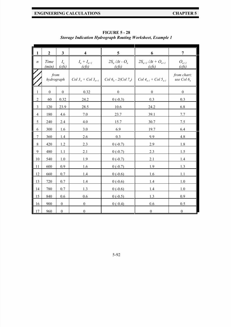
7/30/2019 Virginia Stormwater Managment Handbook Volume_II.pdf
http://slidepdf.com/reader/full/virginia-stormwater-managment-handbook-volumeiipdf 214/354
ENGINEERING CALCULATIONS CHAPTER 5
5-92
FIGURE 5 - 28
Storage Indication Hydrograph Routing Worksheet, Example 1
1 2 3 4 5 6 7
n Time
(min)
I n(cfs)
I n + I n+1
(cfs)
2S n / ∆t - On
(cfs)
2S n+1 / ∆t + On+1
(cfs)
On+1
(cfs)
from
hydrograph Col 3n + Col 3n+1 Col 6 n - 2(Col 7 n ) Col 4n-1 + Col 5n-1
from chart;
use Col 6 n
1 0 0 0.32 0 0 0
2 60 0.32 24.2 0 (-0.3) 0.3 0.3
3 120 23.9 28.5 10.6 24.2 6.8
4 180 4.6 7.0 23.7 39.1 7.7
5 240 2.4 4.0 15.7 30.7 7.5
6 300 1.6 3.0 6.9 19.7 6.4
7 360 1.4 2.6 0.3 9.9 4.8
8 420 1.2 2.3 0 (-0.7) 2.9 1.8
9 480 1.1 2.1 0 (-0.7) 2.3 1.5
10 540 1.0 1.9 0 (-0.7) 2.1 1.4
11 600 0.9 1.6 0 (-0.7) 1.9 1.3
12 660 0.7 1.4 0 (-0.6) 1.6 1.1
13 720 0.7 1.4 0 (-0.6) 1.4 1.0
14 780 0.7 1.3 0 (-0.6) 1.4 1.0
15 840 0.6 0.6 0 (-0.5) 1.3 0.9
16 900 0 0 0 (-0.4) 0.6 0.5
17 960 0 0 0 0
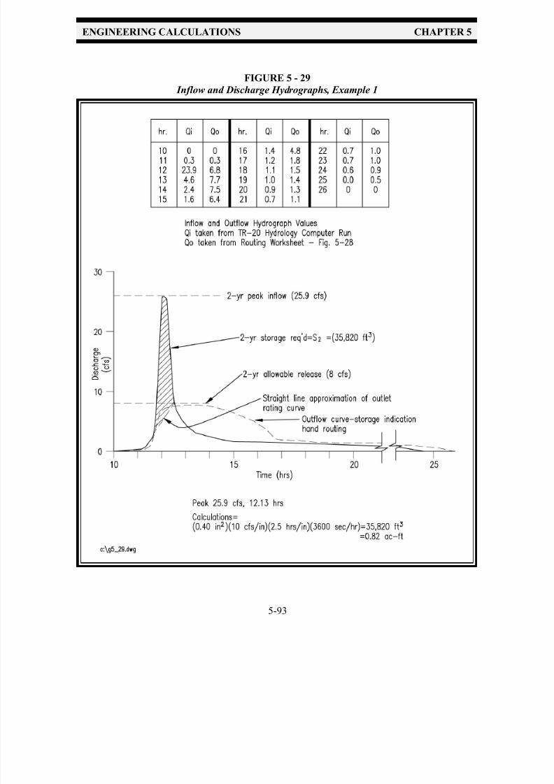
7/30/2019 Virginia Stormwater Managment Handbook Volume_II.pdf
http://slidepdf.com/reader/full/virginia-stormwater-managment-handbook-volumeiipdf 215/354
ENGINEERING CALCULATIONS CHAPTER 5
5-93
FIGURE 5 - 29
Inflow and Discharge Hydrographs, Example 1

7/30/2019 Virginia Stormwater Managment Handbook Volume_II.pdf
http://slidepdf.com/reader/full/virginia-stormwater-managment-handbook-volumeiipdf 216/354
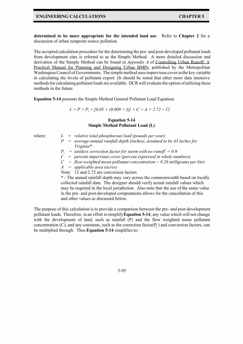
7/30/2019 Virginia Stormwater Managment Handbook Volume_II.pdf
http://slidepdf.com/reader/full/virginia-stormwater-managment-handbook-volumeiipdf 217/354
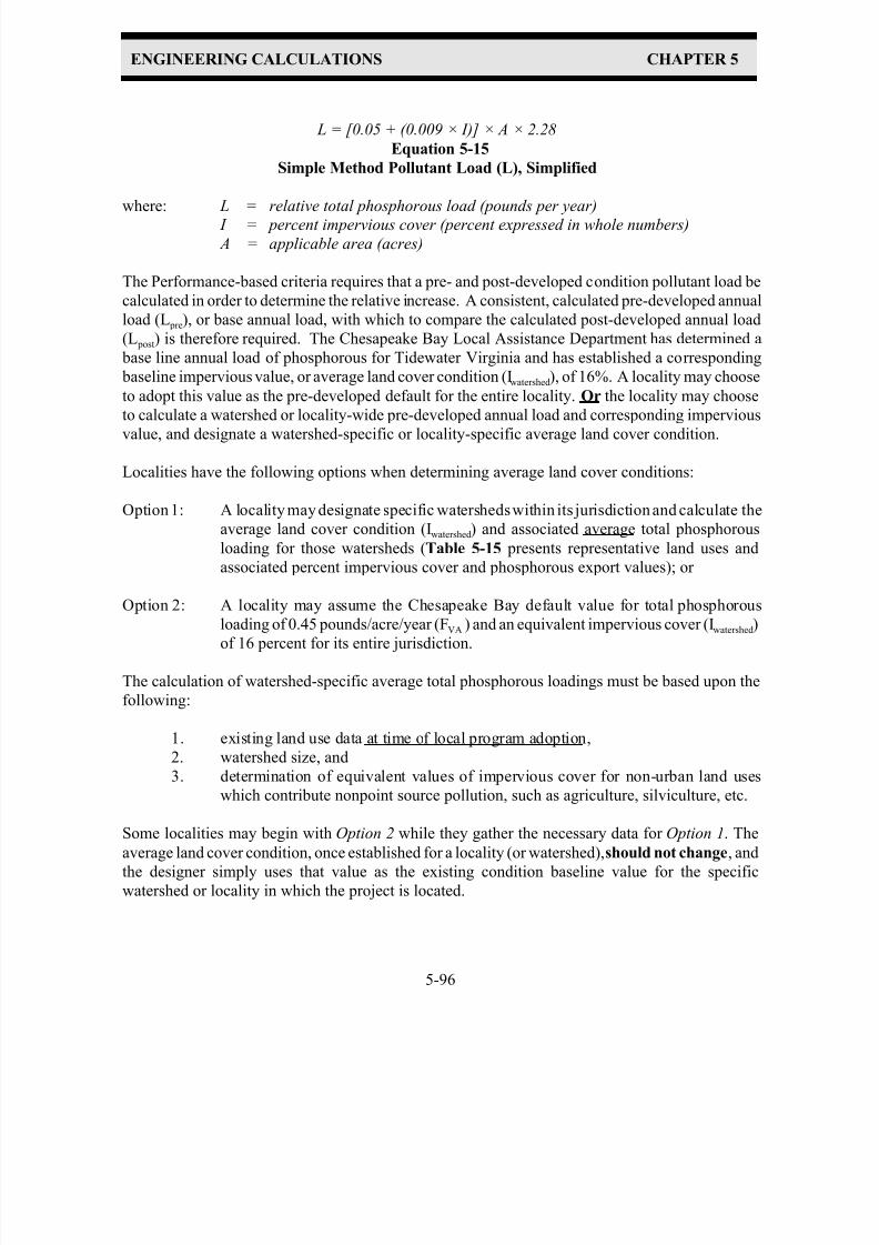
7/30/2019 Virginia Stormwater Managment Handbook Volume_II.pdf
http://slidepdf.com/reader/full/virginia-stormwater-managment-handbook-volumeiipdf 218/354
ENGINEERING CALCULATIONS CHAPTER 5
5-96
L = [0.05 + (0.009 × I)] × A × 2.28
Equation 5-15
Simple Method Pollutant Load (L), Simplified
where: L = relative total phosphorous load (pounds per year) I = percent impervious cover (percent expressed in whole numbers)
A = applicable area (acres)
The Performance-based criteria requires that a pre- and post-developed condition pollutant load be
calculated in order to determine the relative increase. A consistent, calculated pre-developed annual
load (L pre), or base annual load, with which to compare the calculated post-developed annual load
(L post) is therefore required. The Chesapeake Bay Local Assistance Department has determined a
base line annual load of phosphorous for Tidewater Virginia and has established a corresponding
baseline impervious value, or average land cover condition (Iwatershed), of 16%. A locality may choose
to adopt this value as the pre-developed default for the entire locality. Or the locality may choose
to calculate a watershed or locality-wide pre-developed annual load and corresponding imperviousvalue, and designate a watershed-specific or locality-specific average land cover condition.
Localities have the following options when determining average land cover conditions:
Option 1: A locality may designate specific watersheds within its jurisdiction and calculate the
average land cover condition (Iwatershed) and associated average total phosphorous
loading for those watersheds (Table 5-15 presents representative land uses and
associated percent impervious cover and phosphorous export values); or
Option 2: A locality may assume the Chesapeake Bay default value for total phosphorous
loading of 0.45 pounds/acre/year (FVA ) and an equivalent impervious cover (Iwatershed)of 16 percent for its entire jurisdiction.
The calculation of watershed-specific average total phosphorous loadings must be based upon the
following:
1. existing land use data at time of local program adoption,
2. watershed size, and
3. determination of equivalent values of impervious cover for non-urban land uses
which contribute nonpoint source pollution, such as agriculture, silviculture, etc.
Some localities may begin with Option 2 while they gather the necessary data for Option 1. Theaverage land cover condition, once established for a locality (or watershed), should not change, and
the designer simply uses that value as the existing condition baseline value for the specific
watershed or locality in which the project is located.
7/30/2019 Virginia Stormwater Managment Handbook Volume_II.pdf
http://slidepdf.com/reader/full/virginia-stormwater-managment-handbook-volumeiipdf 219/354

7/30/2019 Virginia Stormwater Managment Handbook Volume_II.pdf
http://slidepdf.com/reader/full/virginia-stormwater-managment-handbook-volumeiipdf 220/354
ENGINEERING CALCULATIONS CHAPTER 5
5-98
Post-development Impervious Cover (I post )
The designer must determine the amount of post-development impervious cover (I post), in percent,
within the applicable area. The zoning classifications or proposed density of a site will allow the
designer to estimate impervious cover. It is important that the roadways, sidewalks, and other publicor common ground improvements are included in the overall total impervious cover calculations
when calculating the average lot size and the associated impervious cover. Compliance and final
engineering calculations, however, should be based on impervious cover shown on the final site or
subdivision plan. A locality may set minimum acceptable impervious percentages for particular
land uses, and may also require a determination of the actual proposed impervious cover and use the
higher value. Representative land use categories and associated average impervious cover values
are shown in Table 5-15.
STEP 2 Determine the existing impervious cover (Iexisting) or use the average land cover
condition (Iwatershed) as determined by the locality.
Existing Impervious Cover (Iexisting):
The existing impervious cover (Iexisting) is the percentage of the site that is occupied by impervious
cover prior to the development of the proposed project. For new construction there is typically no
existing impervious cover and therefore the average land cover condition or the watershed-specific
value is used. Two of the four development situations presented in this standard, however, are based
on the presence of existing site features or previous development and use the existing impervious
cover as the basis for determining the pre-development total phosphorous load (L pre).
Average Land Cover Condition (Iwatershed):
A locality must establish the base pollutant load for specific watersheds or for the locality as a whole
based on all of the land uses within the established boundary and, in turn, must determine the
corresponding average land cover condition (Iwatershed) measured in percent impervious cover. The
average land cover condition, therefore, will be a watershed- or locality-specific value, or the
Chesapeake Bay default value of 16%. The average land cover condition, once established for a
locality (or watershed), should not change, and the designer simply uses that value as the pre-
developed or existing average land cover condition for the specific watershed or locality in which
the project is located.
STEP 3 Determine the appropriate development situation.
The performance-based criteria is applied through the use of four development situations. The
application of each of these situations uses the same development characteristic (impervious cover)
to determine the post-development pollutant load (L post). However, the pre-development pollutant
load (L pre) is determined using either the average land cover condition (Iwatershed) or the

7/30/2019 Virginia Stormwater Managment Handbook Volume_II.pdf
http://slidepdf.com/reader/full/virginia-stormwater-managment-handbook-volumeiipdf 221/354
ENGINEERING CALCULATIONS CHAPTER 5
5-99
existing impervious cover (Iexisting), depending on the development situation. The situations are as
follows:
Situation 1: Land development where the existing percent impervious cover (Iexisting) is less than
or equal to the average land cover condition (Iwatershed) and the proposedimprovements will create a total percent impervious cover (I post) which is less than
the average land cover condition (Iwatershed).
Requirement: No reduction in the after development pollutant discharge (L post) is
required.
Situation 2: Land development where the existing percent impervious cover (Iexisting) is less than
or equal to the average land cover condition (Iwatershed) and the proposed
improvements will create a total percent impervious cover (I post) which is greater than
the average land cover condition (Iwatershed).
Requirement: The pollutant discharge after development (L post) shall not exceed the
existing pollutant discharge based on the average land cover condition (L pre(watershed)).
Situation 3: Land development where the existing percent impervious cover (Iexisting) is greater
than the average land cover condition (Iwatershed).
Requirement: The pollutant discharge after development (L post) shall not exceed
1) the pollutant discharge based on existing conditions (L pre(existing)) less 10%; or 2)
the pollutant discharge based on the average land cover condition (L pre(watershed)),
whichever is greater.
Situation 4: Land development where the existing percent impervious cover (Iexisting) is served by
an existing stormwater management BMP(s) that addresses water quality.
Requirement: The pollutant discharge after development (L post) shall not exceed the
existing pollutant discharge based on the existing percent impervious cover while
served by the existing BMP (L pre(existingBMP)). The existing BMP shall be shown to
have been designed and constructed in accordance with proper design standards and
specifications, and to be in proper functioning condition.
If the proposed development meets the criteria for development Situation 1, than the low
density development is considered to be the BMP and no pollutant removal is required. Thecalculation procedure for Situation 1 stops here. Development Situations 2 through 4 proceed
to STEP 4.

7/30/2019 Virginia Stormwater Managment Handbook Volume_II.pdf
http://slidepdf.com/reader/full/virginia-stormwater-managment-handbook-volumeiipdf 222/354
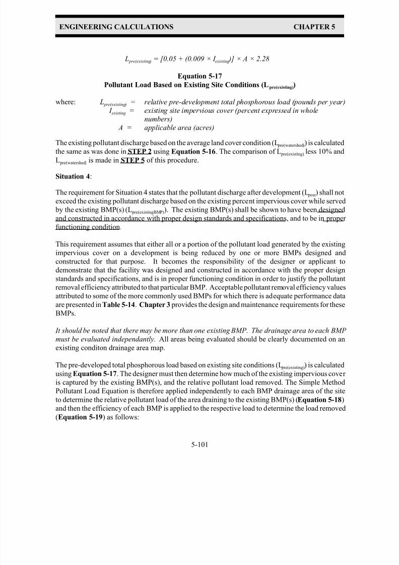
7/30/2019 Virginia Stormwater Managment Handbook Volume_II.pdf
http://slidepdf.com/reader/full/virginia-stormwater-managment-handbook-volumeiipdf 223/354

7/30/2019 Virginia Stormwater Managment Handbook Volume_II.pdf
http://slidepdf.com/reader/full/virginia-stormwater-managment-handbook-volumeiipdf 224/354
ENGINEERING CALCULATIONS CHAPTER 5
5-102
L pre(BMP) = [0.05 + (0.009 × I pre(BMP) )] × AexistBMP × 2.28
Equation 5-18
Pollutant Load to Existing BMP (Lpre(BMP))
where: L pre(BMP) = relative pre-development total phosphorous load entering existing
BMP (pounds per year)
I pre(BMP) = existing impervious cover to existing BMP (percent expressed in
whole numbers)
AexistBMP = drainage area to existing BMP (acres)
The relative pollutant load removed by the existing BMP (Lremoved(existingBMP)) is determined as
follows:
Lremoved(existingBMP) = L pre(BMP) × EFF existBMP
Equation 5-19
Pollutant Load Removed by Existing BMP (Lremoved(existingBMP) )
where: Lremoved(existingBMP) = relative pre-development total phosphorous load removed by
existing BMP (pounds per year)
L pre(BMP) = relative pre-development total phosphorous load entering existing
BMP, Equation 5-18 (pounds per year)
EFF existBMP = documented pollutant removal efficiency of existing BMP
(expressed in decimal form)
Equations 5-18 and 5-19 are thus applied independantly to each existing BMP on the site.
The relative pre-development pollutant load from the site can now be calculated using Equation 5-
20 as follows:
L pre(existingBMP) = L pre(existing) ( Lremoved(existingBMP1) + Lremoved(existingBMP2) + Lremoved(existingBMP3) )
Equation 5-20
Pollutant Load Based on Existing BMP Removal Efficiency (Lpre(existingBMP))
where: L pre(existingBMP) = relative pre-development total phosphorous load while being
served by an existing BMP (pounds per year)
L pre(existing) = relative pre-development total phosphorous load based on existing site conditions, Equation 5-17 (pounds per year)
EFF existBMP = documented pollutant removal efficiency of existing BMP
(expressed in decimal form)
Lremoved(existingBMP) = relative pre-development total phosphorous load removed by
existing BMP, Equation 5-19 (pounds per year)

7/30/2019 Virginia Stormwater Managment Handbook Volume_II.pdf
http://slidepdf.com/reader/full/virginia-stormwater-managment-handbook-volumeiipdf 225/354

7/30/2019 Virginia Stormwater Managment Handbook Volume_II.pdf
http://slidepdf.com/reader/full/virginia-stormwater-managment-handbook-volumeiipdf 226/354
ENGINEERING CALCULATIONS CHAPTER 5
5-104
as the accepted pollutant removal efficiencies for generally acceptable BMPs, are discussed in
Chapter 3: BMP Minimum Standards.
The first step in determining which BMP may satisfy the pollutant removal requirement is to
determine the necessary BMP pollutant removal efficiency. When the entire development is to beserved by one BMP, this can be calculated using the following equation:
EFF = ( RR ÷ L post ) × 100
Equation 5-22
Required Pollutant Removal Efficiency (EFF)
where: EFF = required pollutant removal efficiency
RR = pollutant removal requirement (pounds per year)
L post = relative post-development total phosphorous load, Equation 5-21
(pounds per year)
If more than one BMP will be used on the site, the removal requirement (RR) and post-development
total load (L post) must be calculated for each area using Equation 5-22. The designer can then use
the required pollutant removal efficiency (RR) value to make a preliminary BMP(s) selection from
Table 5-15. This is a preliminary selection since the specific siting and design criteria for the
selected BMP must now be satisfied. Refer to Chapter 3 for more information.
Once the BMP is selected and sited the designer must verify that the BMP(s) satisfies the removal
requirement (RR) for the development. This is done by applying the pollutant removal efficiency
(EFFBMP) of the selected BMP to the post-developed pollutant load entering the BMP as sited
(LBMP). If the entire site drains to the proposed BMP, then the post-development pollutant loadentering the BMP (LBMP) is that which was calculated in STEP 5 (L post = LBMP). In many cases,
however, the topographic constraints of the site, or siting constraints of the specific BMP chosen,
may result in some impervious areas not draining to the proposed BMP. Therefore, the Simple
Method General Pollutant Load Equation must be applied to the actual drainage area of the BMP(s)
as follows:
L BMP = [0.05 + (0.009 × I BMP )] × A propBMP × 2.28
Equation 5-23
Pollutant Load Entering Proposed BMP (LBMP)
where: L BMP = relative post-development total phosphorous load entering proposed BMP(pounds per year)
I BMP = post-development percent impervious cover to proposed BMP
(percent expressed in whole numbers)
A propBMP = drainage area to proposed BMP (acres)

7/30/2019 Virginia Stormwater Managment Handbook Volume_II.pdf
http://slidepdf.com/reader/full/virginia-stormwater-managment-handbook-volumeiipdf 227/354
ENGINEERING CALCULATIONS CHAPTER 5
5-105
The load removed by the BMP is then calculated as follows:
Lremoved = Eff BMP × L BMP
Equation 5-24Pollutant Load Removed by Proposed BMP (Lremoved)
where: Lremoved = post-development total phosphorous load removed by proposed
BMP (pounds per year)
Eff BMP = pollutant removal efficiency of BMP (expressed in decimal form)
L BMP = relative post-development total phosphorous load entering
proposed BMP, Equation 5-23 (pounds per year)
The calculation in this step is performed for each BMP and the various Lremoved values for the
existing and proposed BMPs are summed for the total pollutant load removal as follows:
Lremoved/total = Lremoved/BMP1 + Lremoved/BMP2 + Lremoved/BMP3 + . . .
+ Lremoved(existingBMP1) + Lremoved(existingBMP2) + Lremoved(existingBMP3)
Equation 5-25
Total Pollutant Load Removed by Proposed BMPs (Lremoved/total)
where: Lremoved/total = total pollutant load removed by proposed BMPs (pounds per year)
Lremoved/BMP1 = pollutant load removed by proposed BMP No. 1, Equation 5-24
Lremoved/BMP2 = pollutant load removed by proposed BMP No. 2, Equation 5-24
Lremoved/BMP3 = pollutant load removed by proposed BMP No. 3, Equation 5-24
Lremoved(existingBMP) = pollutant load removed by existing BMP No. 1, Equation 5-19Lremoved(existingBMP) = pollutant load removed by existing BMP No. 2, Equation 5-19
Lremoved(existingBMP) = pollutant load removed by existing BMP No. 3, Equation 5-19
The BMP or combination of BMPs is determined to be adequate if the total pollutant load removed
(L removed/total) is greater than or equal to the removal requirement (RR) calculated in STEP 6:
Lremoved/total RR
If the total load removed is less than the removal requirement (RR) than an alternate BMP or
combination of BMPs must be selected. It may be possible to simply increase the drainage area to
the BMP(s) (if the entire site does not already drain to the BMP) in order to increase the overall
pollutant removal from the site. Another option may be to reduce the impervious cover of thedevelopment in order to lower the removal requirement. The designer may also investigate the
opportunities to capture off-site impervious area drainage in the proposed BMP to compensate for
on-site areas which cannot be captured. In all cases the designer should contact the local program
authority to determine if options are available in the local program as a result of a watershed or
regional BMP plan.
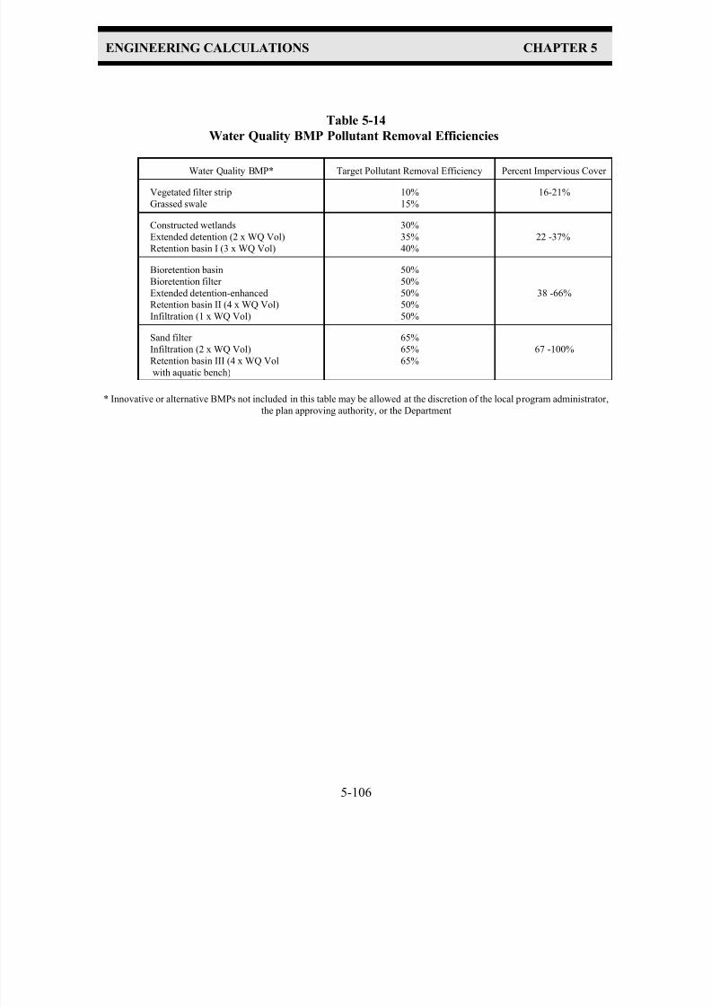
7/30/2019 Virginia Stormwater Managment Handbook Volume_II.pdf
http://slidepdf.com/reader/full/virginia-stormwater-managment-handbook-volumeiipdf 228/354
ENGINEERING CALCULATIONS CHAPTER 5
5-106
Table 5-14
Water Quality BMP Pollutant Removal Efficiencies
Water Quality BMP* Target Pollutant Removal Efficiency Percent Impervious Cover
Vegetated filter strip
Grassed swale
10%
15%
16-21%
Constructed wetlands
Extended detention (2 x WQ Vol)
Retention basin I (3 x WQ Vol)
30%
35%
40%
22 -37%
Bioretention basin
Bioretention filter
Extended detention-enhanced
Retention basin II (4 x WQ Vol)
Infiltration (1 x WQ Vol)
50%
50%
50%
50%
50%
38 -66%
Sand filter Infiltration (2 x WQ Vol)
Retention basin III (4 x WQ Vol
with aquatic bench)
65%65%
65%
67 -100%
* Innovative or alternative BMPs not included in this table may be allowed at the discretion of the local program administrator,
the plan approving authority, or the Department
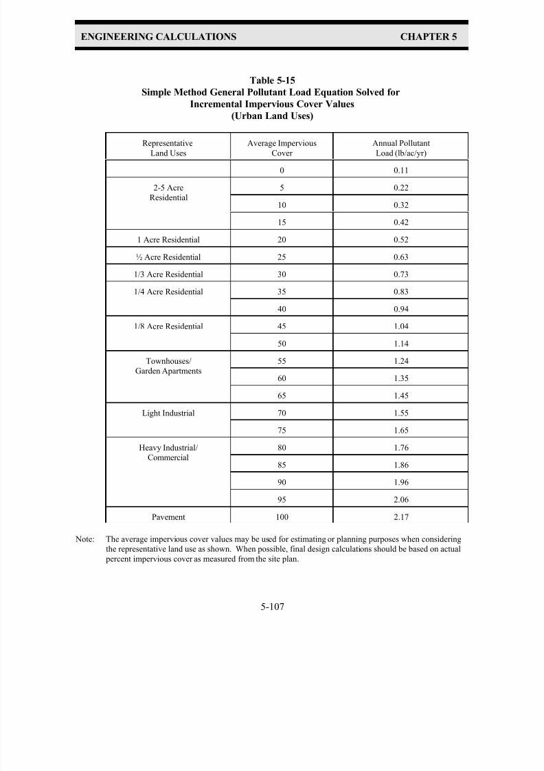
7/30/2019 Virginia Stormwater Managment Handbook Volume_II.pdf
http://slidepdf.com/reader/full/virginia-stormwater-managment-handbook-volumeiipdf 229/354

7/30/2019 Virginia Stormwater Managment Handbook Volume_II.pdf
http://slidepdf.com/reader/full/virginia-stormwater-managment-handbook-volumeiipdf 230/354

7/30/2019 Virginia Stormwater Managment Handbook Volume_II.pdf
http://slidepdf.com/reader/full/virginia-stormwater-managment-handbook-volumeiipdf 231/354
CHAPTER 5
APPENDIX

7/30/2019 Virginia Stormwater Managment Handbook Volume_II.pdf
http://slidepdf.com/reader/full/virginia-stormwater-managment-handbook-volumeiipdf 232/354
APPENDIX 5A
a b Constants for Virginia

7/30/2019 Virginia Stormwater Managment Handbook Volume_II.pdf
http://slidepdf.com/reader/full/virginia-stormwater-managment-handbook-volumeiipdf 233/354

7/30/2019 Virginia Stormwater Managment Handbook Volume_II.pdf
http://slidepdf.com/reader/full/virginia-stormwater-managment-handbook-volumeiipdf 234/354

7/30/2019 Virginia Stormwater Managment Handbook Volume_II.pdf
http://slidepdf.com/reader/full/virginia-stormwater-managment-handbook-volumeiipdf 235/354
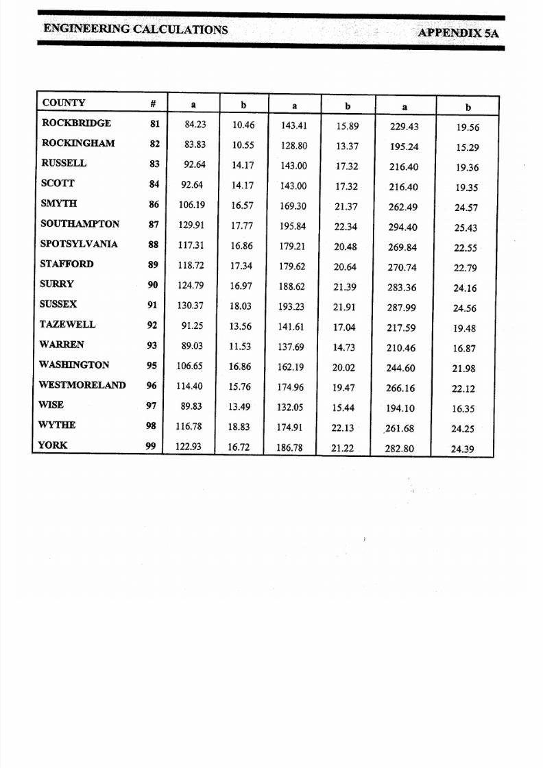
7/30/2019 Virginia Stormwater Managment Handbook Volume_II.pdf
http://slidepdf.com/reader/full/virginia-stormwater-managment-handbook-volumeiipdf 236/354

7/30/2019 Virginia Stormwater Managment Handbook Volume_II.pdf
http://slidepdf.com/reader/full/virginia-stormwater-managment-handbook-volumeiipdf 237/354

7/30/2019 Virginia Stormwater Managment Handbook Volume_II.pdf
http://slidepdf.com/reader/full/virginia-stormwater-managment-handbook-volumeiipdf 238/354
APPENDIX 5B
Filter and Drainage Diaphragm Design
USDA-SCS Soil Mechanics Note No. 1: Guide for Determining the Gradation of
Sand and Gravel Filters (AVAILABLE UPON REQUEST)
USDA-SCS Soil Mechanics Note No. 3: Soil Mechanics Considerations for
Embankment Drains (AVAILABLE UPON REQUEST)
7/30/2019 Virginia Stormwater Managment Handbook Volume_II.pdf
http://slidepdf.com/reader/full/virginia-stormwater-managment-handbook-volumeiipdf 239/354
APPENDIX 5C
Water Balance Analysis
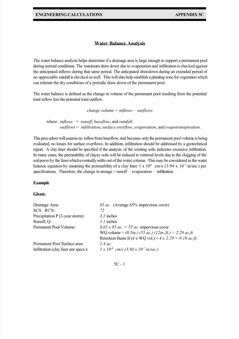
7/30/2019 Virginia Stormwater Managment Handbook Volume_II.pdf
http://slidepdf.com/reader/full/virginia-stormwater-managment-handbook-volumeiipdf 240/354
ENGINEERING CALCULATIONS APPENDIX 5C
5C - 1
Water Balance Analysis
The water balance analysis helps determine if a drainage area is large enough to support a permanent pool
during normal conditions. The maximum draw down due to evaporation and infiltration is checked against
the anticipated inflows during that same period. The anticipated drawdown during an extended period of
no appreciable rainfall is checked as well. This will also help establish a planting zone for vegetation which
can tolerate the dry conditions of a periodic draw down of the permanent pool.
The water balance is defined as the change in volume of the permenant pool resulting from the potential
total inflow less the potential total outflow.
change volume = inflows ! outflows
where: inflows = runoff , baseflow, and rainfall .
outflows = infiltration, surface overflow, evaporation, and evapotranspiration.
This procedure will assume no inflow from baseflow, and because only the permanent pool volume is being
evaluated, no losses for surface overflows. In addition, infiltration should be addressed by a geotechnical
report. A clay liner should be specified if the analysis of the existing soils indicates excessive infiltration.
In many cases, the permeability of clayey soils will be reduced to minimal levels due to the clogging of the
soil pores by the fines which eventually settle out of the water column. This may be considered in the water
balance equation by assuming the permeability of a clay liner: 1 x 10⁻⁶ cm/s (3.94 x 10⁻⁷ in/sec.) per
specifications. Therefore, the change in storage = runoff !
evaporation!
infiltration.
Example
Given:
Drainage Area: 85 ac. (Average 65% impervious cover)
SCS RCN: 72
Precipitation P (2-year storm): 3.1 inches
Runoff, Q: 1.1 inches
Permanent Pool Volume: 0.65 x 85 ac. = 55 ac. impervious cover WQ volume = (0.5in.) (55 ac.) (12in./ft.) = 2.29 ac.ft.
Retention Basin II (4 x WQ vol.) = 4 x 2.29 = 9.16 ac.ft.
Permanent Pool Surface area: 2.4 ac.
Infiltration (clay liner per specs.): 1 x 10⁻⁶ cm/s (3.94 x 10⁻⁷ in/sec.)
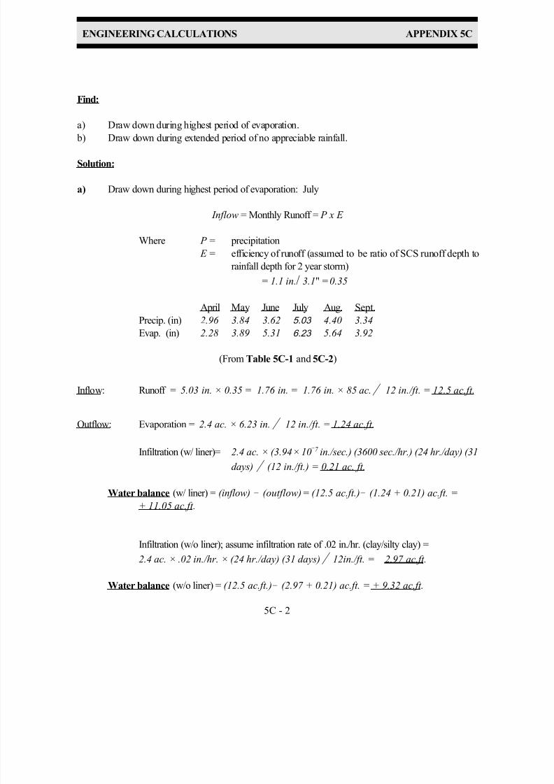
7/30/2019 Virginia Stormwater Managment Handbook Volume_II.pdf
http://slidepdf.com/reader/full/virginia-stormwater-managment-handbook-volumeiipdf 241/354
ENGINEERING CALCULATIONS APPENDIX 5C
5C - 2
Find:
a) Draw down during highest period of evaporation.
b) Draw down during extended period of no appreciable rainfall.
Solution:
a) Draw down during highest period of evaporation: July
Inflow = Monthly Runoff = P x E
Where P = precipitation
E = efficiency of runoff (assumed to be ratio of SCS runoff depth to
rainfall depth for 2 year storm)
= 1.1 in./ 3.1" = 0.35
April May June July Aug. Sept.
Precip. (in) 2.96 3.84 3.62 5.03 4.40 3.34
Evap. (in) 2.28 3.89 5.31 6.23 5.64 3.92
(From Table 5C-1 and 5C-2)
Inflow: Runoff = 5.03 in. × 0.35 = 1.76 in. = 1.76 in. × 85 ac.' 12 in./ft. = 12.5 ac.ft.
Outflow: Evaporation = 2.4 ac. × 6.23 in.' 12 in./ft. = 1.24 ac.ft.
Infiltration (w/ liner)= 2.4 ac. × (3.94 × 10G7 in./sec.) (3600 sec./hr.) (24 hr./day) (31
days) ' (12 in./ft.) = 0.21 ac. ft.
Water balance (w/ liner) = (inflow) ! (outflow) = (12.5 ac.ft.)! (1.24 + 0.21) ac.ft. =
+ 11.05 ac.ft.
Infiltration (w/o liner); assume infiltration rate of .02 in./hr. (clay/silty clay) =
2.4 ac. × .02 in./hr. × (24 hr./day) (31 days) ' 12in./ft. = 2.97 ac.ft.
Water balance (w/o liner) = (12.5 ac.ft.)! (2.97 + 0.21) ac.ft. = + 9.32 ac.ft.
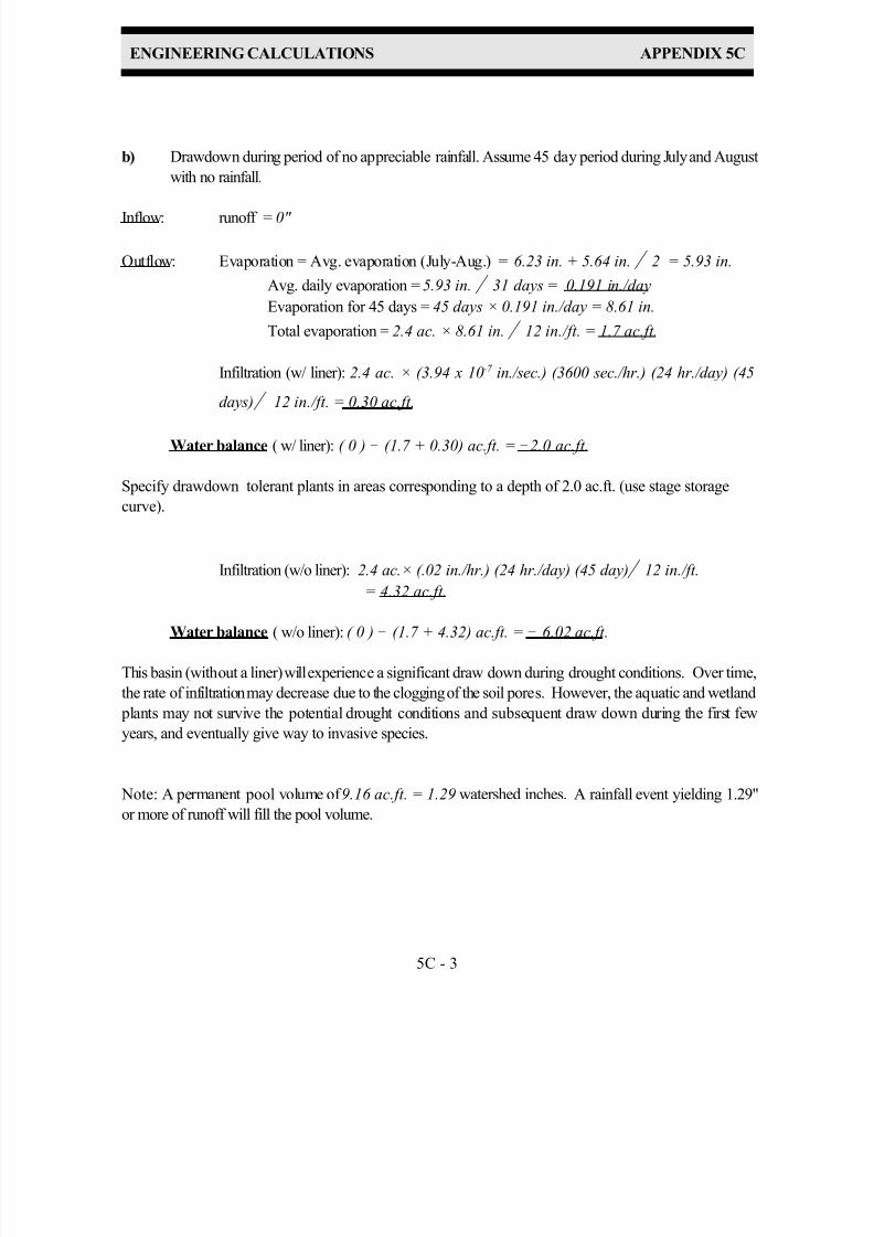
7/30/2019 Virginia Stormwater Managment Handbook Volume_II.pdf
http://slidepdf.com/reader/full/virginia-stormwater-managment-handbook-volumeiipdf 242/354
ENGINEERING CALCULATIONS APPENDIX 5C
5C - 3
b) Drawdown during period of no appreciable rainfall. Assume 45 day period during July and August
with no rainfall.
Inflow: runoff = 0"
Outflow: Evaporation = Avg. evaporation (July-Aug.) = 6.23 in. + 5.64 in. ' 2 = 5.93 in.
Avg. daily evaporation = 5.93 in.' 31 days = 0.191 in./day
Evaporation for 45 days = 45 days × 0.191 in./day = 8.61 in.
Total evaporation = 2.4 ac. × 8.61 in.' 12 in./ft. = 1.7 ac.ft.
Infiltration (w/ liner): 2.4 ac. × (3.94 x 10⁻⁷ in./sec.) (3600 sec./hr.) (24 hr./day) (45
days)'
12 in./ft. = 0.30 ac.ft.
Water balance ( w/ liner): ( 0 ) ! (1.7 + 0.30) ac.ft. = !2.0 ac.ft.
Specify drawdown tolerant plants in areas corresponding to a depth of 2.0 ac.ft. (use stage storage
curve).
Infiltration (w/o liner): 2.4 ac.× (.02 in./hr.) (24 hr./day) (45 day)' 12 in./ft.
= 4.32 ac.ft.
Water balance ( w/o liner): ( 0 ) ! (1.7 + 4.32) ac.ft. = ! 6.02 ac.ft.
This basin (with out a liner) will experience a significant draw down during drought conditions. Over time,
the rate of infiltration may decrease due to the clogging of the soil pores. However, the aquatic and wetland
plants may not survive the potential drought conditions and subsequent draw down during the first few
years, and eventually give way to invasive species.
Note: A permanent pool volume of 9.16 ac.ft. = 1.29 watershed inches. A rainfall event yielding 1.29"
or more of runoff will fill the pool volume.
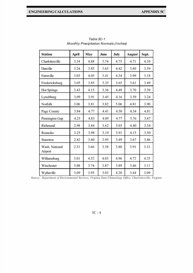
7/30/2019 Virginia Stormwater Managment Handbook Volume_II.pdf
http://slidepdf.com/reader/full/virginia-stormwater-managment-handbook-volumeiipdf 243/354
ENGINEERING CALCULATIONS APPENDIX 5C
5C - 4
Table 5C-1
Monthly Precipitation Normals (I nches)
Station April May June July August Sept.
Charlottesville 3.34 4.88 3.74 4.75 4.71 4.10
Danville 3.24 3.85 3.65 4.42 3.80 3.39
Farmville 3.03 4.05 3.41 4.34 3.99 3.18
Fredericksburg 3.05 3.85 3.35 3.65 3.61 3.49
Hot Springs 3.43 4.15 3.36 4.49 3.70 3.39
Lynchburg 3.09 3.91 3.45 4.16 3.59 3.24
Norfolk 3.06 3.81 3.82 5.06 4.81 3.90
Page County 3.84 4.77 4.41 4.50 4.34 4.81
Pennington Gap 4.25 4.83 4.09 4.77 3.76 3.67
Richmond 2.98 3.84 3.62 5.03 4.40 3.34
Roanoke 3.25 3.98 3.19 3.91 4.15 3.50
Staunton 2.82 3.60 2.95 3.49 3.67 3.46
Wash. National
Airport
2.31 3.66 3.38 3.80 3.91 3.31
Williamsburg 3.01 4.52 4.03 4.96 4.72 4.25
Winchester 3.08 3.74 3.87 3.89 3.46 3.11
Wytheville 3.09 3.95 3.03 4.20 3.44 3.09
Source: Department of Environmental Services, Virginia State Climatology Office, Charlottesville, Virginia

7/30/2019 Virginia Stormwater Managment Handbook Volume_II.pdf
http://slidepdf.com/reader/full/virginia-stormwater-managment-handbook-volumeiipdf 244/354
ENGINEERING CALCULATIONS APPENDIX 5C
5C - 5
Table 5C-2
Potential Evapotranspiration (Inches) *
Station April May June July August Sept.
Charlottesville 2.24 3.84 5.16 6.04 5.45 3.87
Danville 2.35 3.96 5.31 6.23 5.69 3.91
Farmville 2.34 3.81 5.13 6.00 5.41 3.71
Fredericksburg 2.11 3.80 5.23 6.11 5.46 3.83
Hot Springs 1.94 3.41 4.50 5.14 4.69 3.33
Lynchburg 2.21 3.72 4.99 5.85 5.31 3.70
Norfolk 2.20 3.80 5.37 6.34 5.79 4.14
Page County 1.68 3.06 4.09 4.71 4.26 3.05
Pennington Gap 2.14 3.59 4.72 5.45 4.97 3.60
Richmond 2.28 3.89 5.31 6.23 5.64 3.92
Roanoke 2.20 3.75 4.99 5.85 5.30 3.67
Staunton 2.00 3.52 4.77 5.52 4.95 3.47
Wash. National
Airport
2.13 3.87 5.50 6.51 5.84 4.06
Williamsburg 2.27 3.86 5.23 6.14 5.61 3.97
Winchester 2.07 3.68 4.99 5.82 5.26 3.67
Wytheville 2.01 3.43 4.46 5.17 4.71 3.39
Source:Department of Environmental Services, Virginia State Climatology Office, Charlottesville, Virginia
* Calculated using the Thornthwaite method
7/30/2019 Virginia Stormwater Managment Handbook Volume_II.pdf
http://slidepdf.com/reader/full/virginia-stormwater-managment-handbook-volumeiipdf 245/354
APPENDIX 5D
Worksheets Stage Storage Worksheet
Stage-Storage-Discharge Worksheet
Storage Indication Hydrograph Routing Worksheet; 2S/ ∆t + O Vs. O
Storage Indication Hydrograph Routing Worksheet
Performance-Based Water Quality Calculations Worksheet 1
Performance-Based Water Quality Calculations Worksheet 2: Situation 2
Performance-Based Water Quality Calculations Worksheet 3: Situation 3
Performance-Based Water Quality Calculations Worksheet 4: Situation 4

7/30/2019 Virginia Stormwater Managment Handbook Volume_II.pdf
http://slidepdf.com/reader/full/virginia-stormwater-managment-handbook-volumeiipdf 246/354
ENGINEERING CALCULATIONS APPENDIX 5D
5D - 1
Stage-Storage Worksheet
PROJECT: SHEET OF
COUNTY: COMPUTED BY: DATE:
DESCRIPTION:
ATTACH COPY OF TOPO: SCALE - 1" = ft .
1 2 3 4 5 6 7 8
ELEV.AREA
(in2 )
AREA
(ft 2 )
AVG.
AREA
(ft 2 )
INTERVALVOL.
(ft 3 )
TOTAL VOLUME
(ft 3 ) (ac.ft .)
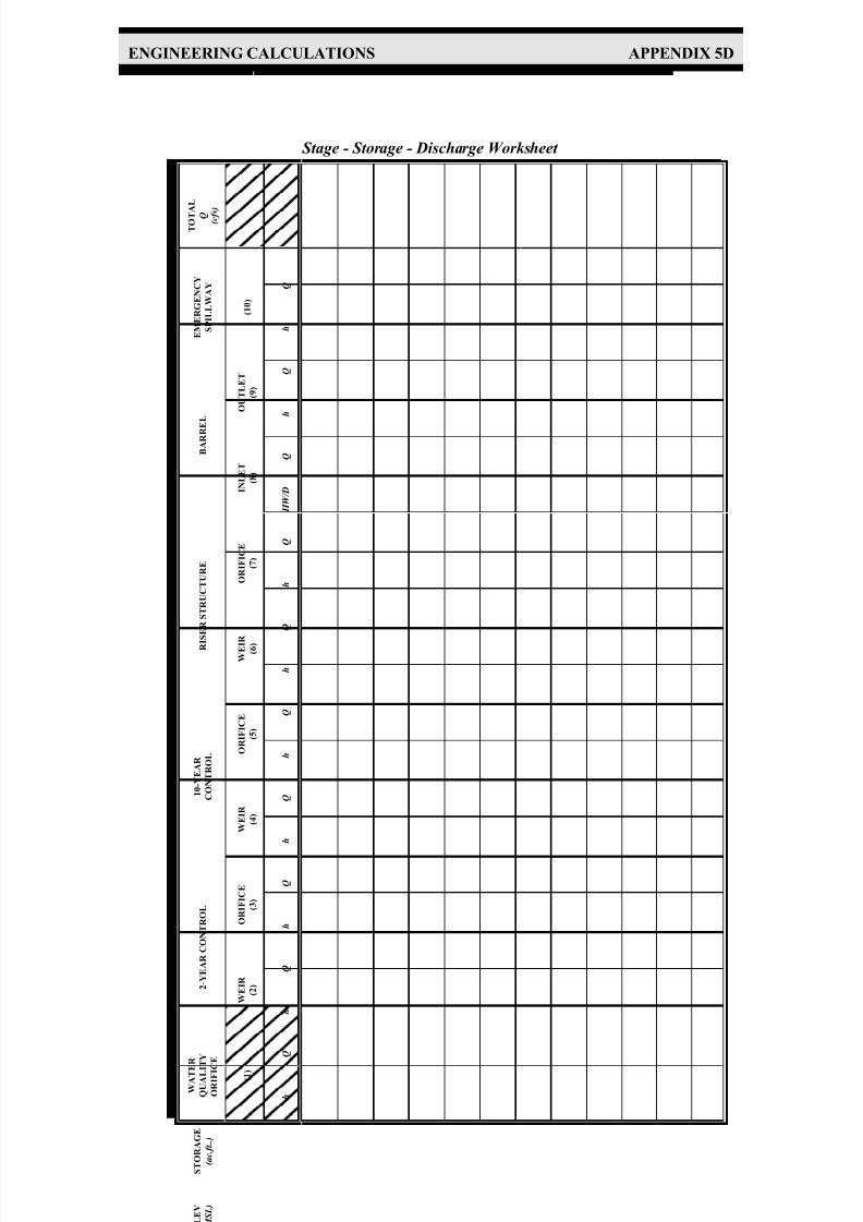
7/30/2019 Virginia Stormwater Managment Handbook Volume_II.pdf
http://slidepdf.com/reader/full/virginia-stormwater-managment-handbook-volumeiipdf 247/354
ENGINEERING CALCULATIONS APPENDIX 5D
Y E
2 - Y E A R C O N T R O L
1 0 - Y E A R
C O N T R O L
R I S E R S T
R U C T U R E
B A R R E L
E M E R G E N C Y
S P I L L W A Y
T O T A L
Q ( c f s )
W E I R
( 2 )
O R I F I C E
( 3 )
W E I R ( 4 )
O R I F I C E
( 5 )
W E I R
( 6 )
O R I F I C E
( 7 )
I N L E T
( 8 )
O
U T L E T
( 9 )
( 1 0 )
Q
h
Q
h
Q
h
Q
h
Q
h
Q
h
Q
H W / D
Q
h
Q
h
Q
Stage - Storage - Discharge Worksheet
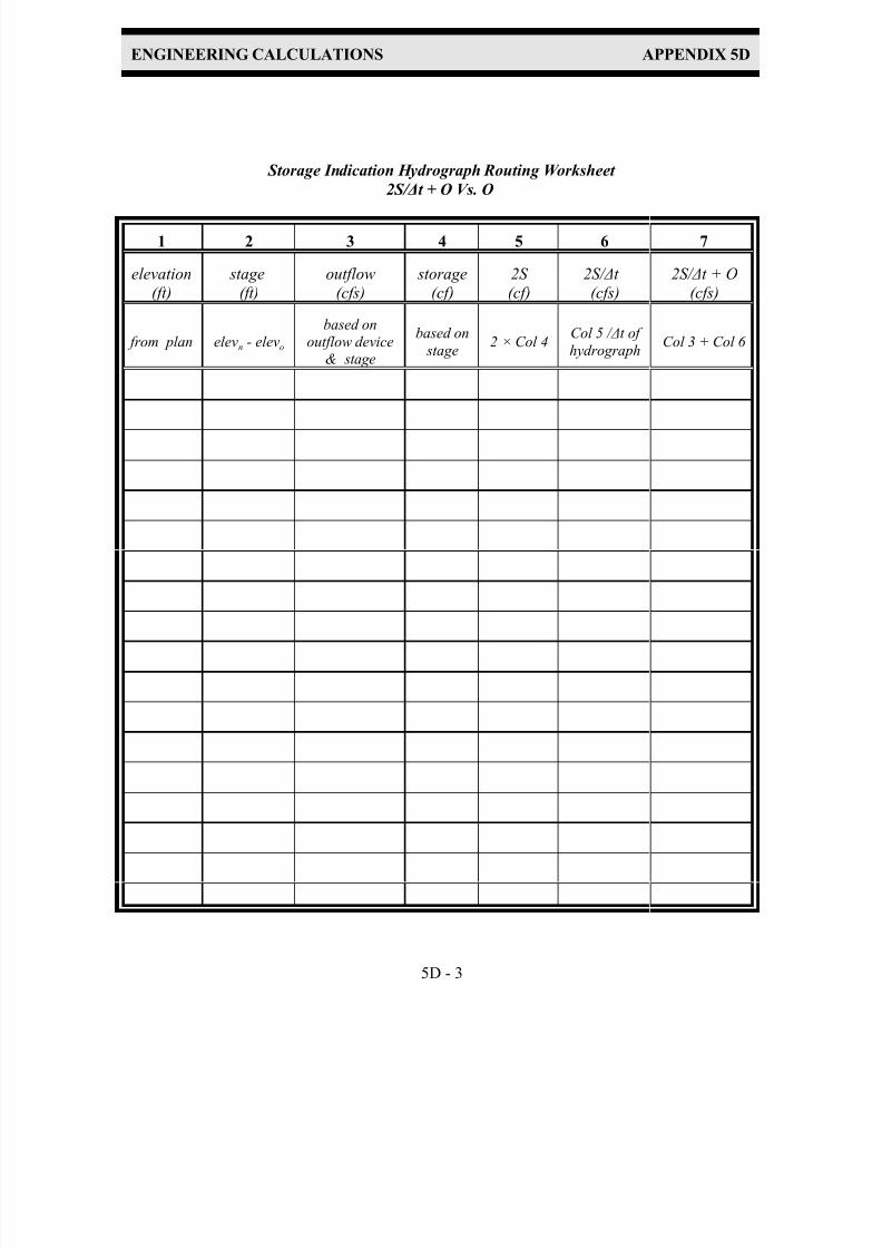
7/30/2019 Virginia Stormwater Managment Handbook Volume_II.pdf
http://slidepdf.com/reader/full/virginia-stormwater-managment-handbook-volumeiipdf 248/354
ENGINEERING CALCULATIONS APPENDIX 5D
5D - 3
Storage Indication Hydrograph Routing Worksheet
2S/ ∆t + O Vs. O
1 2 3 4 5 6 7
elevation
(ft)
stage
(ft)
outflow
(cfs)
storage
(cf)
2S
(cf)
2S/ ∆t
(cfs)
2S/ ∆t + O
(cfs)
from plan elevn - elevo
based on
outflow device
& stage
based on
stage2 × Col 4
Col 5 / ∆t of
hydrographCol 3 + Col 6
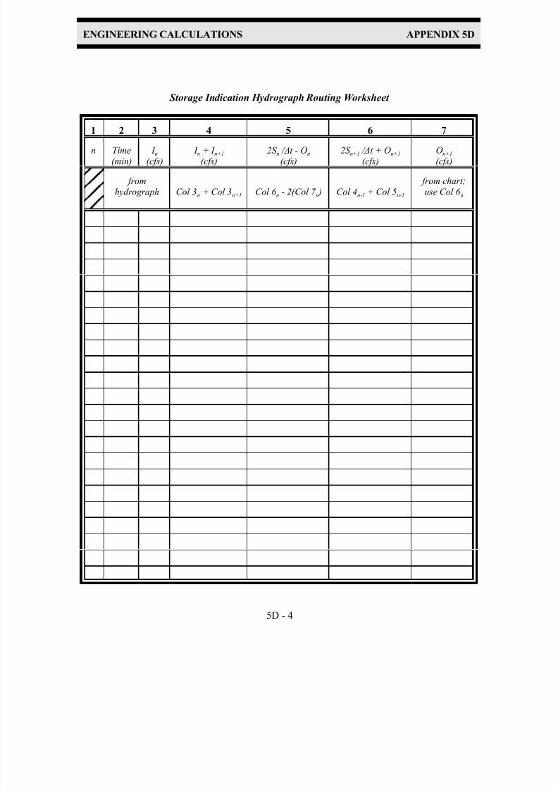
7/30/2019 Virginia Stormwater Managment Handbook Volume_II.pdf
http://slidepdf.com/reader/full/virginia-stormwater-managment-handbook-volumeiipdf 249/354
ENGINEERING CALCULATIONS APPENDIX 5D
5D - 4
Storage Indication Hydrograph Routing Worksheet
1 2 3 4 5 6 7
n Time
(min)
I n(cfs)
I n + I n+1
(cfs)
2S n / ∆t - On
(cfs)
2S n+1 / ∆t + On+1
(cfs)
On+1
(cfs)
from
hydrograph Col 3n + Col 3n+1 Col 6 n - 2(Col 7 n ) Col 4n-1 + Col 5n-1
from chart;
use Col 6 n
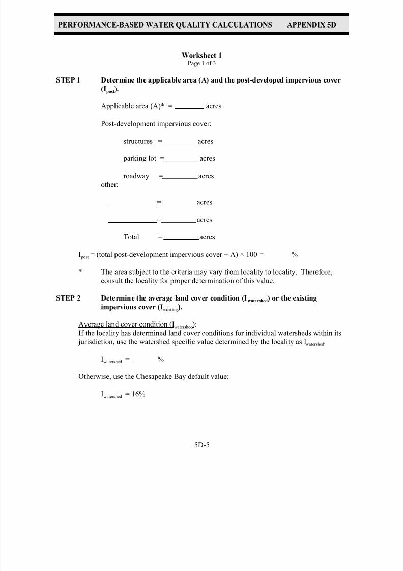
7/30/2019 Virginia Stormwater Managment Handbook Volume_II.pdf
http://slidepdf.com/reader/full/virginia-stormwater-managment-handbook-volumeiipdf 250/354
PERFORMANCE-BASED WATER QUALITY CALCULATIONS APPENDIX 5D
5D-5
Worksheet 1Page 1 of 3
STEP 1 Determine the applicable area (A) and the post-developed impervious cover
(Ipost).
Applicable area (A)* = acres
Post-development impervious cover:
structures = acres
parking lot = acres
roadway = acres
other:
= acres
= acres
Total = acres
I post = (total post-development impervious cover ÷ A) × 100 = %
* The area subject to the criteria may vary from locality to locality. Therefore,
consult the locality for proper determination of this value.
STEP 2 Determine the average land cover condition (Iwatershed) or the existing
impervious cover (Iexisting).
Average land cover condition (Iwatershed):
If the locality has determined land cover conditions for individual watersheds within its
jurisdiction, use the watershed specific value determined by the locality as Iwatershed.
Iwatershed = %
Otherwise, use the Chesapeake Bay default value:
Iwatershed = 16%

7/30/2019 Virginia Stormwater Managment Handbook Volume_II.pdf
http://slidepdf.com/reader/full/virginia-stormwater-managment-handbook-volumeiipdf 251/354
PERFORMANCE-BASED WATER QUALITY CALCULATIONS APPENDIX 5D
5D-6
Worksheet 1Page 2 of 3
Existing impervious cover (Iexisting):
Determine the existing impervious cover of the development site if present.
Existing impervious cover:
structures = acres
parking lot = acres
roadway = acres
other:
= acres
= acres
Total = acres
Iexisting = (total existing impervious cover ÷ A*) × 100 = %
* The area should be the same as used in STEP 1.
STEP 3 Determine the appropriate development situation.
The site information determined in STEP 1 and STEP 2 provide enough information to
determine the appropriate development situation under which the performance criteria will
apply. Check (U ) the appropriate development situation as follows:
Situation 1: This consists of land development where the existing percent impervious
cover (Iexisting) is less than or equal to the average land cover condition
(Iwatershed) and the proposed improvements will create a total percent
impervious cover (I post) which is less than or equal to the average landcover condition (Iwatershed).
Ipost % Iwatershed %

7/30/2019 Virginia Stormwater Managment Handbook Volume_II.pdf
http://slidepdf.com/reader/full/virginia-stormwater-managment-handbook-volumeiipdf 252/354
PERFORMANCE-BASED WATER QUALITY CALCULATIONS APPENDIX 5D
5D-7
Worksheet 1Page 3 of 3
Situation 2: This consists of land development where the existing percent imperviouscover (Iexisting) is less than or equal to the average land cover condition
(Iwatershed) and the proposed improvements will create a total percent
impervious cover (I post) which is greater than the average land cover
condition (Iwatershed).
Iexisting % Iwatershed %; and
Ipost % > Iwatershed %
Situation 3: This consists of land development where the existing percent impervious
cover (Iexisting) is greater than the average land cover condition (Iwatershed).
Iexisting % > Iwatershed %
Situation 4: This consists of land development where the existing percent impervious
cover (Iexisting) is served by an existing stormwater management BMP(s)
that addresses water quality.
If the proposed development meets the criteria for development Situation 1, than the low
density development is considered to be the BMP and no pollutant removal is required.
The calculation procedure for Situation 1 stops here. If the proposed development meetsthe criteria for development Situations 2, 3, or 4, then proceed to STEP 4 on the
appropriate worksheet.

7/30/2019 Virginia Stormwater Managment Handbook Volume_II.pdf
http://slidepdf.com/reader/full/virginia-stormwater-managment-handbook-volumeiipdf 253/354
PERFORMANCE-BASED WATER QUALITY CALCULATIONS APPENDIX 5D
5D-8
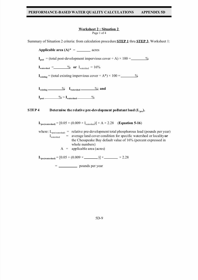
7/30/2019 Virginia Stormwater Managment Handbook Volume_II.pdf
http://slidepdf.com/reader/full/virginia-stormwater-managment-handbook-volumeiipdf 254/354
PERFORMANCE-BASED WATER QUALITY CALCULATIONS APPENDIX 5D
5D-9
Worksheet 2 : Situation 2Page 1 of 4
Summary of Situation 2 criteria: from calculation procedure STEP 1 thru STEP 3, Worksheet 1:
Applicable area (A)* = acres
Ipost = (total post-development impervious cover ÷ A) × 100 = %
Iwatershed = % or Iwatershed = 16%
Iexisting = (total existing impervious cover ÷ A*) × 100 = %
Iexisting % Iwatershed %; and
Ipost % > Iwatershed %
STEP 4 Determine the relative pre-development pollutant load (Lpre).
Lpre(watershed) = [0.05 + (0.009 × Iwatershed)] × A × 2.28 (Equation 5-16)
where: L pre(watershed) = relative pre-development total phosphorous load (pounds per year)
Iwatershed = average land cover condition for specific watershed or locality or
the Chesapeake Bay default value of 16% (percent expressed inwhole numbers)
A = applicable area (acres)
Lpre(watershed) = [0.05 + (0.009 × )] × × 2.28
= pounds per year

7/30/2019 Virginia Stormwater Managment Handbook Volume_II.pdf
http://slidepdf.com/reader/full/virginia-stormwater-managment-handbook-volumeiipdf 255/354
PERFORMANCE-BASED WATER QUALITY CALCULATIONS APPENDIX 5D
5D-10
Worksheet 2 : Situation 2Page 2 of 4
STEP 5 Determine the relative post-development pollutant load (Lpost).
Lpost = [0.05 + (0.009 × I post)] × A × 2.28 (Equation 5-21)
where: L post = relative post-development total phosphorous load (pounds per
year)
I post = post-development percent impervious cover (percent expressed in
whole numbers)
A = applicable area (acres)
Lpost = [0.05 + (0.009 × )] × × 2.28
= pounds per year
STEP 6 Determine the relative pollutant removal requirement (RR).
RR = L post L pre(watershed)
RR =
= pounds per year
STEP 7 Identify best management practice (BMP) for the site.
1. Determine the required pollutant removal efficiency for the site:
EFF = ( RR ÷ L post ) × 100 (Equation 5-22)
where: EFF = required pollutant removal efficiency (percent expressed in whole
numbers)
RR = pollutant removal requirement (pounds per year)
L post = relative post-development total phosphorous load (pounds per year)
EFF = ( ÷ ) × 100
= %

7/30/2019 Virginia Stormwater Managment Handbook Volume_II.pdf
http://slidepdf.com/reader/full/virginia-stormwater-managment-handbook-volumeiipdf 256/354
PERFORMANCE-BASED WATER QUALITY CALCULATIONS APPENDIX 5D
5D-11
Worksheet 2 : Situation 2Page 3 of 4
2. Select BMP(s) from Table 5-15 and locate on the site:
BMP 1:
BMP 2:
BMP 3:
3. Determine the pollutant load entering the proposed BMP(s):
LBMP = [0.05 + (0.009 × IBMP)] × A × 2.28 (Equation 5-23)
where: LBMP = relative post-development total phosphorous load entering
proposed BMP (pounds per year)
IBMP = post-development percent impervious cover of BMP drainage area
(percent expressed in whole numbers)
A = drainage area of proposed BMP (acres)
LBMP1 = [0.05 + (0.009 × )] × × 2.28
= pounds per year
LBMP2 = [0.05 + (0.009 × )] × × 2.28
= pounds per year
LBMP3 = [0.05 + (0.009 × )] × × 2.28
= pounds per year
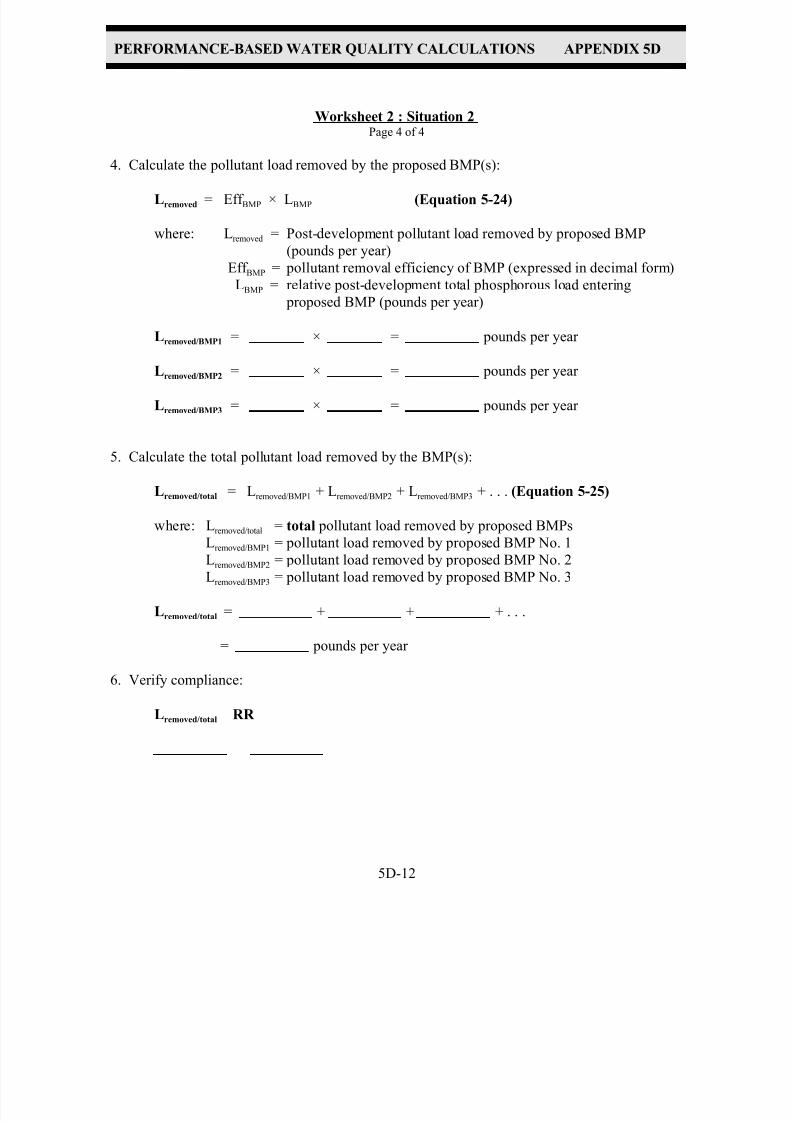
7/30/2019 Virginia Stormwater Managment Handbook Volume_II.pdf
http://slidepdf.com/reader/full/virginia-stormwater-managment-handbook-volumeiipdf 257/354
PERFORMANCE-BASED WATER QUALITY CALCULATIONS APPENDIX 5D
5D-12
Worksheet 2 : Situation 2Page 4 of 4
4. Calculate the pollutant load removed by the proposed BMP(s):
Lremoved = Eff BMP × LBMP (Equation 5-24)
where: Lremoved = Post-development pollutant load removed by proposed BMP
(pounds per year)
Eff BMP = pollutant removal efficiency of BMP (expressed in decimal form)
LBMP = relative post-development total phosphorous load entering
proposed BMP (pounds per year)
Lremoved/BMP1 = × = pounds per year
Lremoved/BMP2 = × = pounds per year
Lremoved/BMP3 = × = pounds per year
5. Calculate the total pollutant load removed by the BMP(s):
Lremoved/total = Lremoved/BMP1 + Lremoved/BMP2 + Lremoved/BMP3 + . . . (Equation 5-25)
where: Lremoved/total = total pollutant load removed by proposed BMPs
Lremoved/BMP1 = pollutant load removed by proposed BMP No. 1
Lremoved/BMP2 = pollutant load removed by proposed BMP No. 2Lremoved/BMP3 = pollutant load removed by proposed BMP No. 3
Lremoved/total = + + + . . .
= pounds per year
6. Verify compliance:
Lremoved/total RR
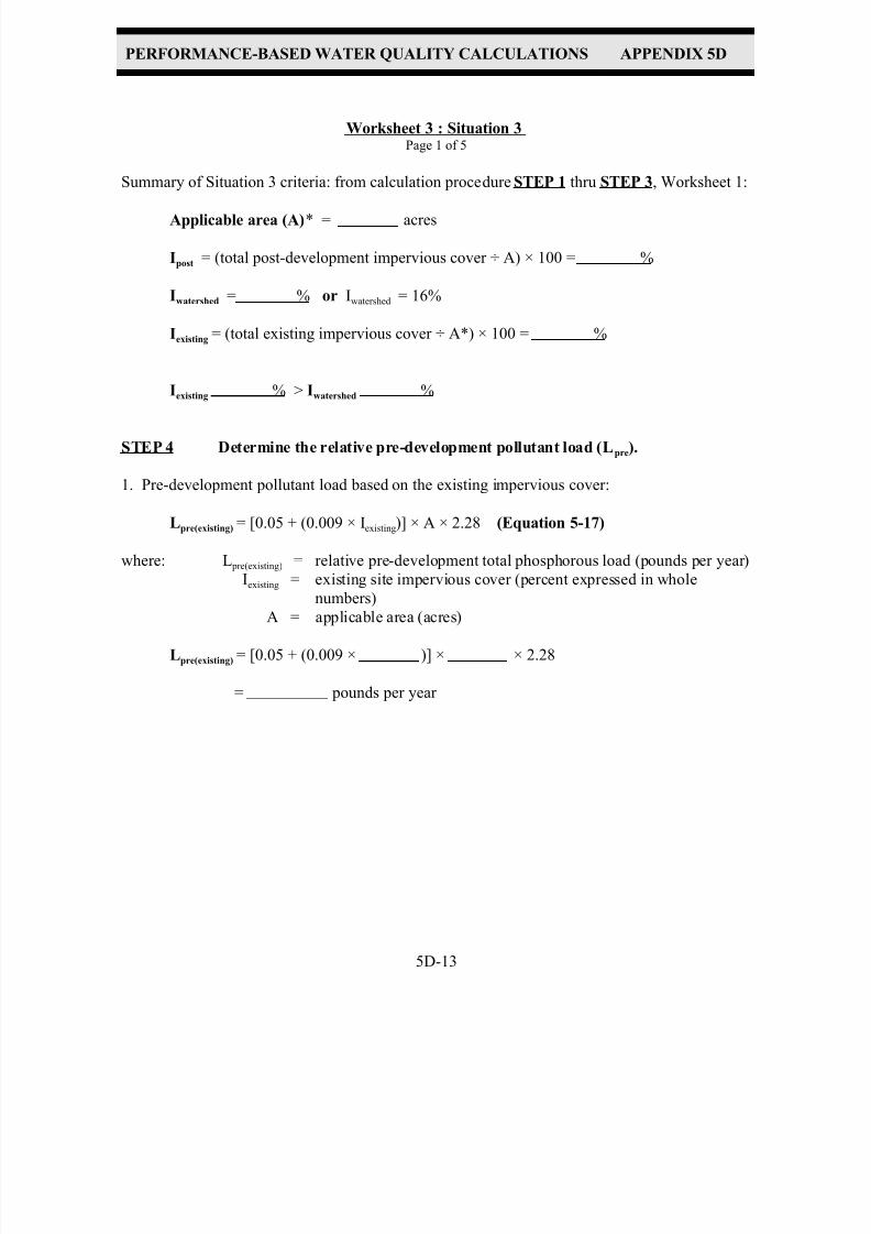
7/30/2019 Virginia Stormwater Managment Handbook Volume_II.pdf
http://slidepdf.com/reader/full/virginia-stormwater-managment-handbook-volumeiipdf 258/354
PERFORMANCE-BASED WATER QUALITY CALCULATIONS APPENDIX 5D
5D-13
Worksheet 3 : Situation 3Page 1 of 5
Summary of Situation 3 criteria: from calculation procedure STEP 1 thru STEP 3, Worksheet 1:
Applicable area (A)* = acres
Ipost = (total post-development impervious cover ÷ A) × 100 = %
Iwatershed = % or Iwatershed = 16%
Iexisting = (total existing impervious cover ÷ A*) × 100 = %
Iexisting % > Iwatershed %
STEP 4 Determine the relative pre-development pollutant load (Lpre).
1. Pre-development pollutant load based on the existing impervious cover:
Lpre(existing) = [0.05 + (0.009 × Iexisting)] × A × 2.28 (Equation 5-17)
where: L pre(existing) = relative pre-development total phosphorous load (pounds per year)
Iexisting = existing site impervious cover (percent expressed in whole
numbers)
A = applicable area (acres)
Lpre(existing) = [0.05 + (0.009 × )] × × 2.28
= pounds per year

7/30/2019 Virginia Stormwater Managment Handbook Volume_II.pdf
http://slidepdf.com/reader/full/virginia-stormwater-managment-handbook-volumeiipdf 259/354
PERFORMANCE-BASED WATER QUALITY CALCULATIONS APPENDIX 5D
5D-14
Worksheet 3 : Situation 3Page 2 of 5
2. Pre-development pollutant load based on the average land cover condition:
Lpre(watershed) = [0.05 + (0.009 × Iwatershed)] × A × 2.28 (Equation 5-16)
where: L pre(watershed) = relative pre-development total phosphorous load (pounds per year)
Iwatershed = average land cover condition for specific watershed or locality or
the Chesapeake Bay default value of 16% (percent expressed in
whole numbers)
A = applicable area (acres)
Lpre(watershed) = [0.05 + (0.009 × )] × × 2.28
= pounds per year
STEP 5 Determine the relative post-development pollutant load (Lpost).
Lpost = [0.05 + (0.009 × I post)] × A × 2.28 (Equation 5-21)
where: L post = relative post-development total phosphorous load (pounds per
year)
I post = post-development percent impervious cover (percent expressed in
whole numbers)
A = applicable area (acres)
Lpost = [0.05 + (0.009 × )] × × 2.28
= pounds per year
STEP 6 Determine the relative pollutant removal requirement (RR).
RR = L post (0.9 × L pre(existing))
= (0.9 × ) = pounds per year or
RR = L post L pre(watershed)
= = pounds per year
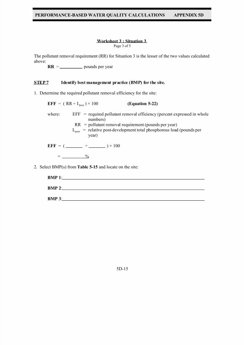
7/30/2019 Virginia Stormwater Managment Handbook Volume_II.pdf
http://slidepdf.com/reader/full/virginia-stormwater-managment-handbook-volumeiipdf 260/354
PERFORMANCE-BASED WATER QUALITY CALCULATIONS APPENDIX 5D
5D-15
Worksheet 3 : Situation 3Page 3 of 5
The pollutant removal requirement (RR) for Situation 3 is the lesser of the two values calculatedabove:
RR = pounds per year
STEP 7 Identify best management practice (BMP) for the site.
1. Determine the required pollutant removal efficiency for the site:
EFF = ( RR ÷ L post ) × 100 (Equation 5-22)
where: EFF = required pollutant removal efficiency (percent expressed in wholenumbers)
RR = pollutant removal requirement (pounds per year)
L post = relative post-development total phosphorous load (pounds per
year)
EFF = ( ÷ ) × 100
= %
2. Select BMP(s) from Table 5-15 and locate on the site:
BMP 1:
BMP 2:
BMP 3:
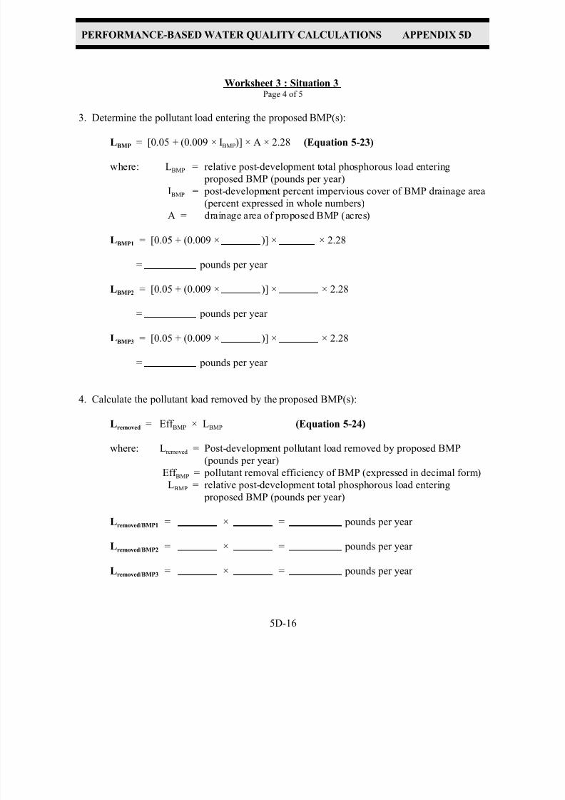
7/30/2019 Virginia Stormwater Managment Handbook Volume_II.pdf
http://slidepdf.com/reader/full/virginia-stormwater-managment-handbook-volumeiipdf 261/354
PERFORMANCE-BASED WATER QUALITY CALCULATIONS APPENDIX 5D
5D-16
Worksheet 3 : Situation 3Page 4 of 5
3. Determine the pollutant load entering the proposed BMP(s):
LBMP = [0.05 + (0.009 × IBMP)] × A × 2.28 (Equation 5-23)
where: LBMP = relative post-development total phosphorous load entering
proposed BMP (pounds per year)
IBMP = post-development percent impervious cover of BMP drainage area
(percent expressed in whole numbers)
A = drainage area of proposed BMP (acres)
LBMP1 = [0.05 + (0.009 × )] × × 2.28
= pounds per year
LBMP2 = [0.05 + (0.009 × )] × × 2.28
= pounds per year
LBMP3 = [0.05 + (0.009 × )] × × 2.28
= pounds per year
4. Calculate the pollutant load removed by the proposed BMP(s):
Lremoved = Eff BMP × LBMP (Equation 5-24)
where: Lremoved = Post-development pollutant load removed by proposed BMP
(pounds per year)
Eff BMP = pollutant removal efficiency of BMP (expressed in decimal form)
LBMP = relative post-development total phosphorous load entering
proposed BMP (pounds per year)
Lremoved/BMP1 = × = pounds per year
Lremoved/BMP2 = × = pounds per year
Lremoved/BMP3 = × = pounds per year

7/30/2019 Virginia Stormwater Managment Handbook Volume_II.pdf
http://slidepdf.com/reader/full/virginia-stormwater-managment-handbook-volumeiipdf 262/354
PERFORMANCE-BASED WATER QUALITY CALCULATIONS APPENDIX 5D
5D-17
Worksheet 3 : Situation 3Page 5 of 5
5. Calculate the total pollutant load removed by the BMP(s):
Lremoved/total = Lremoved/BMP1 + Lremoved/BMP2 + Lremoved/BMP3 + . . . (Equation 5-25)
where: Lremoved/total = total pollutant load removed by proposed BMPs
Lremoved/BMP1 = pollutant load removed by proposed BMP No. 1
Lremoved/BMP2 = pollutant load removed by proposed BMP No. 2
Lremoved/BMP3 = pollutant load removed by proposed BMP No. 3
Lremoved/total = + + + . . .
= pounds per year
6. Verify compliance:
Lremoved/total RR

7/30/2019 Virginia Stormwater Managment Handbook Volume_II.pdf
http://slidepdf.com/reader/full/virginia-stormwater-managment-handbook-volumeiipdf 263/354
PERFORMANCE-BASED WATER QUALITY CALCULATIONS APPENDIX 5D
5D-18
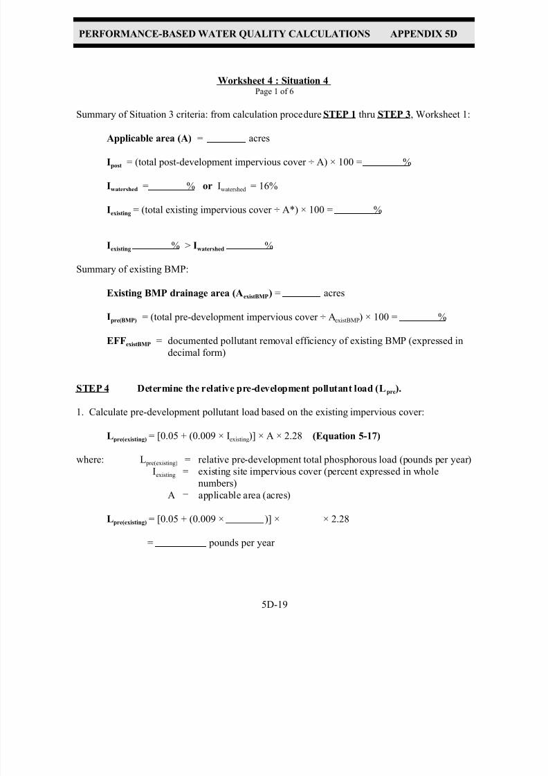
7/30/2019 Virginia Stormwater Managment Handbook Volume_II.pdf
http://slidepdf.com/reader/full/virginia-stormwater-managment-handbook-volumeiipdf 264/354
PERFORMANCE-BASED WATER QUALITY CALCULATIONS APPENDIX 5D
5D-19
Worksheet 4 : Situation 4Page 1 of 6
Summary of Situation 3 criteria: from calculation procedure STEP 1 thru STEP 3, Worksheet 1:
Applicable area (A) = acres
Ipost = (total post-development impervious cover ÷ A) × 100 = %
Iwatershed = % or Iwatershed = 16%
Iexisting = (total existing impervious cover ÷ A*) × 100 = %
Iexisting % > Iwatershed %
Summary of existing BMP:
Existing BMP drainage area (AexistBMP) = acres
Ipre(BMP) = (total pre-development impervious cover ÷ AexistBMP) × 100 = %
EFFexistBMP = documented pollutant removal efficiency of existing BMP (expressed in
decimal form)
STEP 4 Determine the relative pre-development pollutant load (Lpre).
1. Calculate pre-development pollutant load based on the existing impervious cover:
Lpre(existing) = [0.05 + (0.009 × Iexisting)] × A × 2.28 (Equation 5-17)
where: L pre(existing) = relative pre-development total phosphorous load (pounds per year)
Iexisting = existing site impervious cover (percent expressed in whole
numbers)
A = applicable area (acres)
Lpre(existing) = [0.05 + (0.009 × )] × × 2.28
= pounds per year
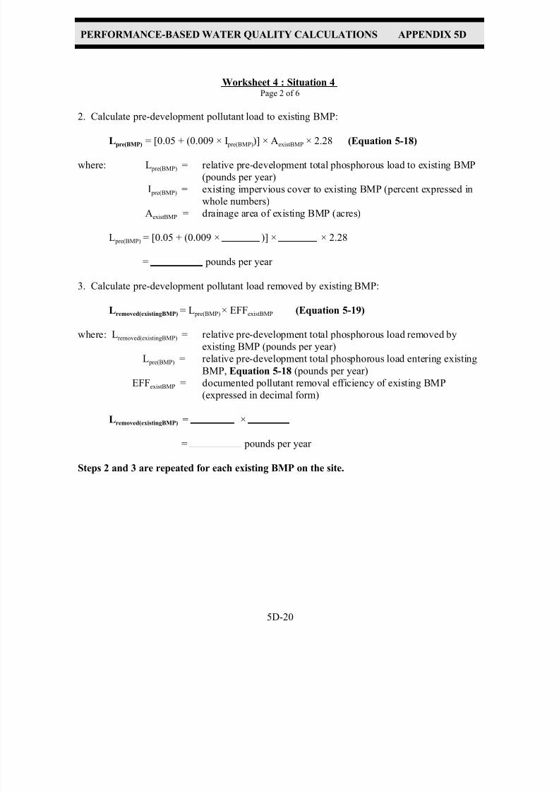
7/30/2019 Virginia Stormwater Managment Handbook Volume_II.pdf
http://slidepdf.com/reader/full/virginia-stormwater-managment-handbook-volumeiipdf 265/354
PERFORMANCE-BASED WATER QUALITY CALCULATIONS APPENDIX 5D
5D-20
Worksheet 4 : Situation 4Page 2 of 6
2. Calculate pre-development pollutant load to existing BMP:
Lpre(BMP) = [0.05 + (0.009 × I pre(BMP))] × AexistBMP × 2.28 (Equation 5-18)
where: L pre(BMP) = relative pre-development total phosphorous load to existing BMP
(pounds per year)
I pre(BMP) = existing impervious cover to existing BMP (percent expressed in
whole numbers)
AexistBMP = drainage area of existing BMP (acres)
L pre(BMP) = [0.05 + (0.009 × )] × × 2.28
= pounds per year
3. Calculate pre-development pollutant load removed by existing BMP:
Lremoved(existingBMP) = L pre(BMP) × EFFexistBMP (Equation 5-19)
where: Lremoved(existingBMP) = relative pre-development total phosphorous load removed by
existing BMP (pounds per year)
L pre(BMP) = relative pre-development total phosphorous load entering existing
BMP, Equation 5-18 (pounds per year)
EFFexistBMP = documented pollutant removal efficiency of existing BMP
(expressed in decimal form)
Lremoved(existingBMP) = ×
= pounds per year
Steps 2 and 3 are repeated for each existing BMP on the site.

7/30/2019 Virginia Stormwater Managment Handbook Volume_II.pdf
http://slidepdf.com/reader/full/virginia-stormwater-managment-handbook-volumeiipdf 266/354
PERFORMANCE-BASED WATER QUALITY CALCULATIONS APPENDIX 5D
5D-21
Worksheet 4: Situation 4Page 3 of 6
4. Calculate the pre-development pollutant load while being served by existing BMP(S):
Lpre(existingBMP) = L pre(existing) ( Lremoved(existingBMP1) + Lremoved(existingBMP2) + Lremoved(existingBMP3) )
Equation 5-20
where: L pre(existingBMP) = relative pre-development total phosphorous load while being
served by an existing BMP (pounds per year)
L pre(existing) = relative pre-development total phosphorous load based on existing
site conditions, Equation 5-17 (pounds per year)
EFFexistBMP = documented pollutant removal efficiency of existing BMP
(expressed in decimal form)
Lremoved(existingBMP) = relative pre-development total phosphorous load removed by
existing BMP, Equation 5-19 (pounds per year)
Lpre(existingBMP) = ( + + )
= pounds per year
STEP 5 Determine the relative post-development pollutant load (Lpost).
Lpost = [0.05 + (0.009 × I post)] × A × 2.28 (Equation 5-21)
where: L post = relative post-development total phosphorous load (pounds per
year)I post = post-development percent impervious cover (percent expressed in
whole numbers)
A = applicable area (acres)
Lpost = [0.05 + (0.009 × )] × × 2.28
= pounds per year
STEP 6 Determine the relative pollutant removal requirement (RR).
RR = L post L pre(existingBMP)
=
RR = pounds per year
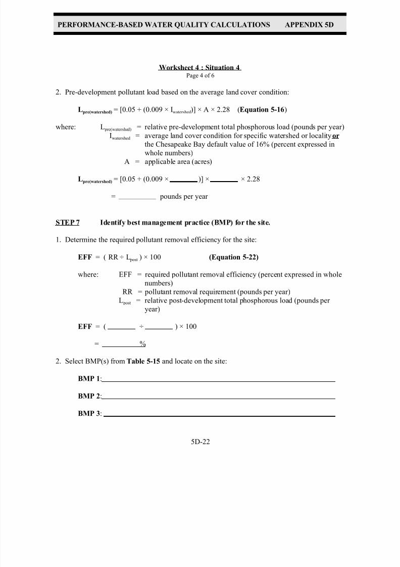
7/30/2019 Virginia Stormwater Managment Handbook Volume_II.pdf
http://slidepdf.com/reader/full/virginia-stormwater-managment-handbook-volumeiipdf 267/354
PERFORMANCE-BASED WATER QUALITY CALCULATIONS APPENDIX 5D
5D-22
Worksheet 4 : Situation 4Page 4 of 6
2. Pre-development pollutant load based on the average land cover condition:
Lpre(watershed) = [0.05 + (0.009 × Iwatershed)] × A × 2.28 (Equation 5-16)
where: L pre(watershed) = relative pre-development total phosphorous load (pounds per year)
Iwatershed = average land cover condition for specific watershed or locality or
the Chesapeake Bay default value of 16% (percent expressed in
whole numbers)
A = applicable area (acres)
Lpre(watershed) = [0.05 + (0.009 × )] × × 2.28
= pounds per year
STEP 7 Identify best management practice (BMP) for the site.
1. Determine the required pollutant removal efficiency for the site:
EFF = ( RR ÷ L post ) × 100 (Equation 5-22)
where: EFF = required pollutant removal efficiency (percent expressed in whole
numbers)RR = pollutant removal requirement (pounds per year)
L post = relative post-development total phosphorous load (pounds per
year)
EFF = ( ÷ ) × 100
= %
2. Select BMP(s) from Table 5-15 and locate on the site:
BMP 1:
BMP 2:
BMP 3:
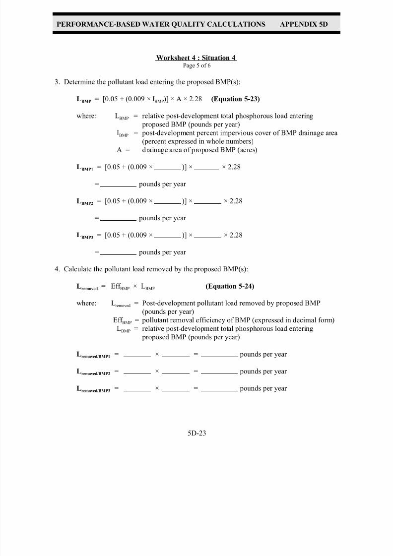
7/30/2019 Virginia Stormwater Managment Handbook Volume_II.pdf
http://slidepdf.com/reader/full/virginia-stormwater-managment-handbook-volumeiipdf 268/354
PERFORMANCE-BASED WATER QUALITY CALCULATIONS APPENDIX 5D
5D-23
Worksheet 4 : Situation 4Page 5 of 6
3. Determine the pollutant load entering the proposed BMP(s):
LBMP = [0.05 + (0.009 × IBMP)] × A × 2.28 (Equation 5-23)
where: LBMP = relative post-development total phosphorous load entering
proposed BMP (pounds per year)
IBMP = post-development percent impervious cover of BMP drainage area
(percent expressed in whole numbers)
A = drainage area of proposed BMP (acres)
LBMP1 = [0.05 + (0.009 × )] × × 2.28
= pounds per year
LBMP2 = [0.05 + (0.009 × )] × × 2.28
= pounds per year
LBMP3 = [0.05 + (0.009 × )] × × 2.28
= pounds per year
4. Calculate the pollutant load removed by the proposed BMP(s):
Lremoved = Eff BMP × LBMP (Equation 5-24)
where: Lremoved = Post-development pollutant load removed by proposed BMP
(pounds per year)
Eff BMP = pollutant removal efficiency of BMP (expressed in decimal form)
LBMP = relative post-development total phosphorous load entering
proposed BMP (pounds per year)
Lremoved/BMP1 = × = pounds per year
Lremoved/BMP2 = × = pounds per year
Lremoved/BMP3 = × = pounds per year
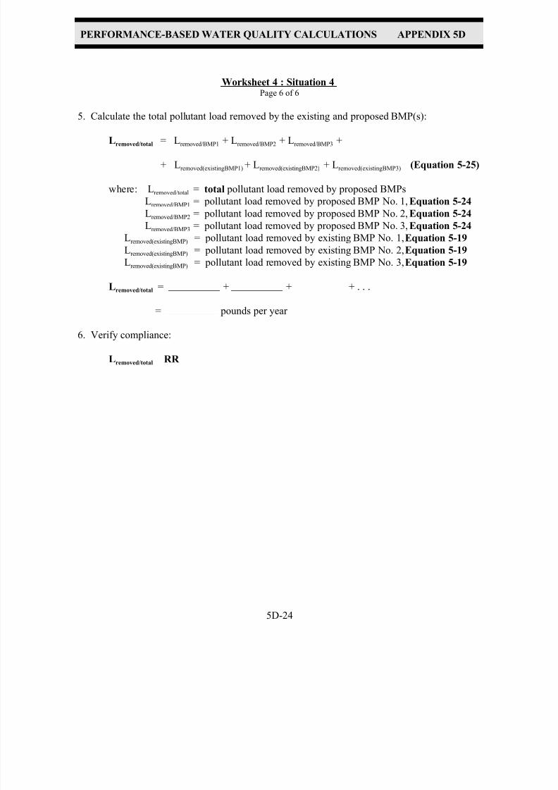
7/30/2019 Virginia Stormwater Managment Handbook Volume_II.pdf
http://slidepdf.com/reader/full/virginia-stormwater-managment-handbook-volumeiipdf 269/354
PERFORMANCE-BASED WATER QUALITY CALCULATIONS APPENDIX 5D
5D-24
Worksheet 4 : Situation 4Page 6 of 6
5. Calculate the total pollutant load removed by the existing and proposed BMP(s):
Lremoved/total = Lremoved/BMP1 + Lremoved/BMP2 + Lremoved/BMP3 +
+ Lremoved(existingBMP1) + Lremoved(existingBMP2) + Lremoved(existingBMP3) (Equation 5-25)
where: Lremoved/total = total pollutant load removed by proposed BMPs
Lremoved/BMP1 = pollutant load removed by proposed BMP No. 1, Equation 5-24
Lremoved/BMP2 = pollutant load removed by proposed BMP No. 2, Equation 5-24
Lremoved/BMP3 = pollutant load removed by proposed BMP No. 3, Equation 5-24
Lremoved(existingBMP) = pollutant load removed by existing BMP No. 1, Equation 5-19
Lremoved(existingBMP) = pollutant load removed by existing BMP No. 2, Equation 5-19
Lremoved(existingBMP) = pollutant load removed by existing BMP No. 3, Equation 5-19
Lremoved/total = + + + . . .
= pounds per year
6. Verify compliance:
Lremoved/total RR

7/30/2019 Virginia Stormwater Managment Handbook Volume_II.pdf
http://slidepdf.com/reader/full/virginia-stormwater-managment-handbook-volumeiipdf 270/354
CHAPTER 6
EXAMPLE PROBLEMS

7/30/2019 Virginia Stormwater Managment Handbook Volume_II.pdf
http://slidepdf.com/reader/full/virginia-stormwater-managment-handbook-volumeiipdf 271/354
Example 6.1
HYDROLOGY
Example 6.1A . . . . . . . . . . . . . . . . . . . . . . . . . . . . . . . . . . . . . . . . . . . . 6.1- 4
Example 6.1B . . . . . . . . . . . . . . . . . . . . . . . . . . . . . . . . . . . . . . . . . . . . 6.1-16
Example 6.1C . . . . . . . . . . . . . . . . . . . . . . . . . . . . . . . . . . . . . . . . . . . . 6.1-18
Example 6.1D . . . . . . . . . . . . . . . . . . . . . . . . . . . . . . . . . . . . . . . . . . . . 6.1-34

7/30/2019 Virginia Stormwater Managment Handbook Volume_II.pdf
http://slidepdf.com/reader/full/virginia-stormwater-managment-handbook-volumeiipdf 272/354
EXAMPLE 6.1 CHAPTER 6
ILLUSTRATIONS
#
FIGURES PAGE
6.1-1a,b Example 1, 25-Acre Watershed Pre- and Post-developed Condition . . . . . . 6.1-3
6.1-1c Example 1, 25-Acre Watershed Post-developed Condition -
Most Representative T c Flow Path . . . . . . . . . . . . . . . . . . . . . . . . . . . . . . . 6.1-4
6.1-2a Example 1, Sub-watersheds 1 & 2 Pre-developed Condition . . . . . . . . . . . . 6.1-19
6.1-2b Example 1, Sub-watersheds 1 & 2 Post-developed Condition . . . . . . . . . . . 6.1-20
# TABLES PAGE
6.1-1 Hydrologic Summary - Full Watershed, Example 6.1A
TR-55 Graphical Peak Discharge Method . . . . . . . . . . . . . . . . . . . . . . . . . . 6.1-5
6.1-2 Hydrologic Summary - Full Watershed, Example 6.1B
Rational Method Peak Discharge, Q=CIA . . . . . . . . . . . . . . . . . . . . . . . . . 6.1-16
6.1-3 Hydrologic Summary - Sub-watersheds, Example 6.1C
SCS TR-55 Tabular Hydrograph Analysis . . . . . . . . . . . . . . . . . . . . . . . . . . 6.1-18
6.1-4 Hydrologic Summary - Sub-watershed 1, Example 6.1D
Rational Method Peak Discharge, Q = CIA . . . . . . . . . . . . . . . . . . . . . . . . 6.1-34

7/30/2019 Virginia Stormwater Managment Handbook Volume_II.pdf
http://slidepdf.com/reader/full/virginia-stormwater-managment-handbook-volumeiipdf 273/354
EXAMPLE 6.1 CHAPTER 6
6.1 - 1
EXAMPLE 6.1
INTRODUCTION
Example 6.1 (referred to as Example 1 in Chapter 5 develops the hydrology of a 25-acre watershed
drained by two distinct channels. A study point is established at the confluence of these channels. The
proposed development disturbs 11.9 acres.
Several design elements are illustrated in this problem. Example 6.1A uses SCS TR-55 methodology
for determining the peak discharge from the watershed. It also shows the impact of the time of
concentration, t c , on the peak discharge.
Example 6.1B uses the Rational Method* for determining the peak discharge from the same
watershed described in 6.1A.
Example 6.1C uses the SCS Tabular Method and divides the watershed into sub-watersheds. The
watershed analyzed in this example is simple, but it serves to illustrate the conditions where a
development may be large enough or diverse enough to warrant the use of sub-watersheds.
Example 6.1D uses the Rational Method to determine the peak discharge from the sub-watersheds
described in 6.1C.
* Note that the 25-acre drainage area exceeds the Rational Method’s recommended limit of 20
acres, but the method is still used in this example for comparison purposes.
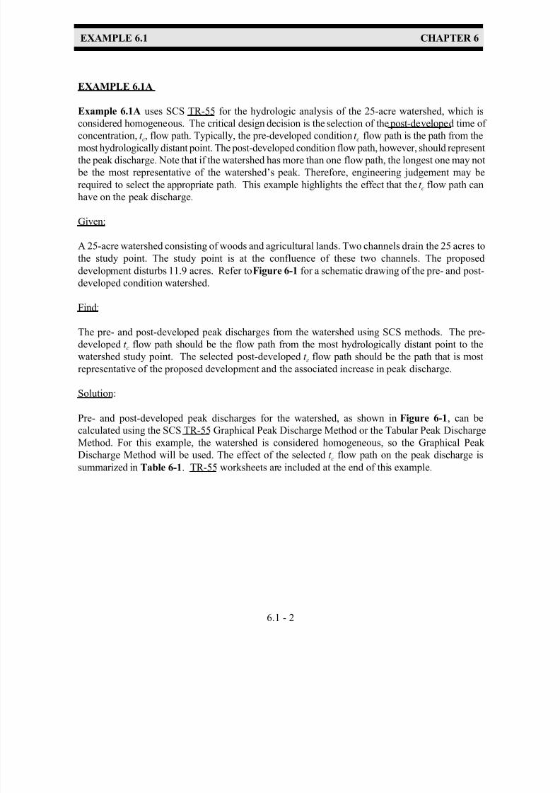
7/30/2019 Virginia Stormwater Managment Handbook Volume_II.pdf
http://slidepdf.com/reader/full/virginia-stormwater-managment-handbook-volumeiipdf 274/354
EXAMPLE 6.1 CHAPTER 6
6.1 - 2
EXAMPLE 6.1A
Example 6.1A uses SCS TR-55 for the hydrologic analysis of the 25-acre watershed, which is
considered homogeneous. The critical design decision is the selection of the post-developed time of
concentration, t c, flow path. Typically, the pre-developed condition t c flow path is the path from themost hydrologically distant point. The post-developed condition flow path, however, should represent
the peak discharge. Note that if the watershed has more than one flow path, the longest one may not
be the most representative of the watershed’s peak. Therefore, engineering judgement may be
required to select the appropriate path. This example highlights the effect that the t c flow path can
have on the peak discharge.
Given:
A 25-acre watershed consisting of woods and agricultural lands. Two channels drain the 25 acres to
the study point. The study point is at the confluence of these two channels. The proposed
development disturbs 11.9 acres. Refer to Figure 6-1 for a schematic drawing of the pre- and post-
developed condition watershed.
Find:
The pre- and post-developed peak discharges from the watershed using SCS methods. The pre-
developed t c flow path should be the flow path from the most hydrologically distant point to the
watershed study point. The selected post-developed t c flow path should be the path that is most
representative of the proposed development and the associated increase in peak discharge.
Solution:
Pre- and post-developed peak discharges for the watershed, as shown in Figure 6-1, can be
calculated using the SCS TR-55 Graphical Peak Discharge Method or the Tabular Peak Discharge
Method. For this example, the watershed is considered homogeneous, so the Graphical Peak
Discharge Method will be used. The effect of the selected t c flow path on the peak discharge is
summarized in Table 6-1. TR-55 worksheets are included at the end of this example.
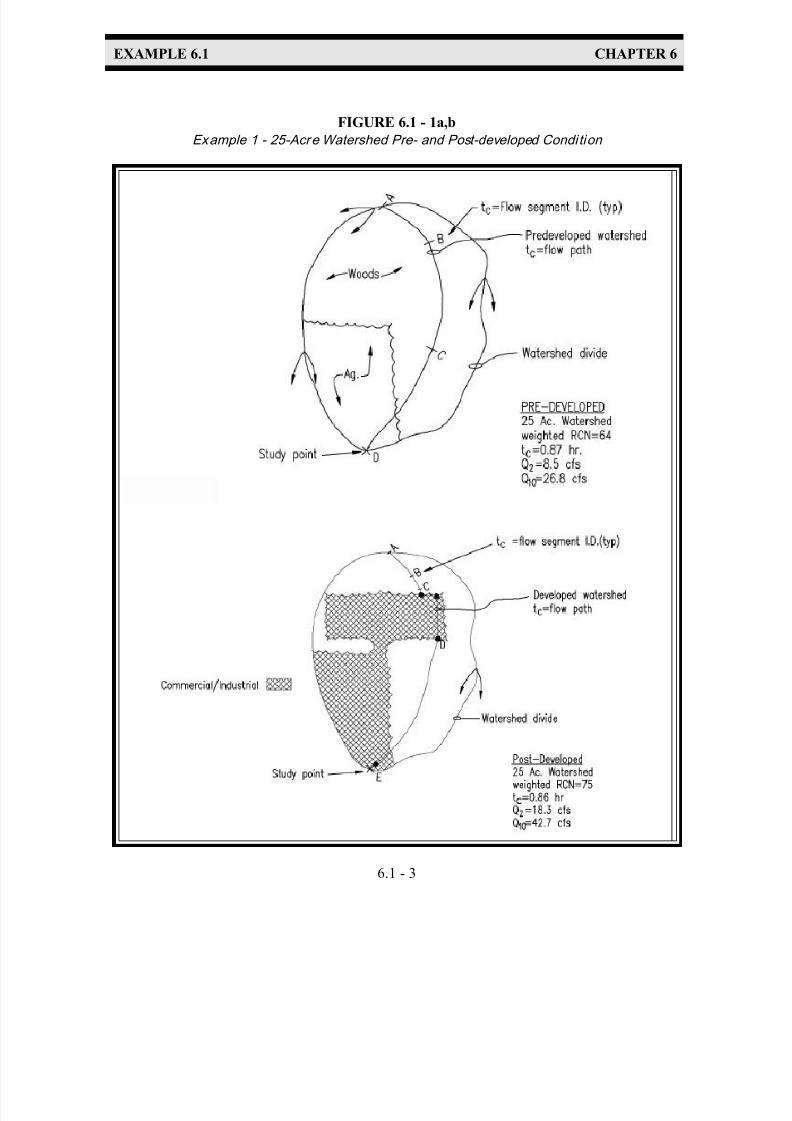
7/30/2019 Virginia Stormwater Managment Handbook Volume_II.pdf
http://slidepdf.com/reader/full/virginia-stormwater-managment-handbook-volumeiipdf 275/354
EXAMPLE 6.1 CHAPTER 6
6.1 - 3
FIGURE 6.1 - 1a,b
Example 1 - 25-Acre Watershed Pre- and Post-developed Condi tion
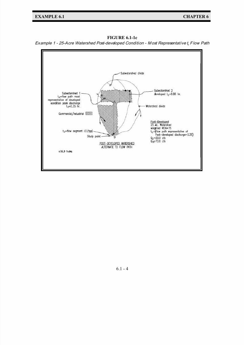
7/30/2019 Virginia Stormwater Managment Handbook Volume_II.pdf
http://slidepdf.com/reader/full/virginia-stormwater-managment-handbook-volumeiipdf 276/354
EXAMPLE 6.1 CHAPTER 6
6.1 - 4
FIGURE 6.1-1c
Example 1 - 25-Acre Watershed Post-developed Condition - Most Representative t c F low Path

7/30/2019 Virginia Stormwater Managment Handbook Volume_II.pdf
http://slidepdf.com/reader/full/virginia-stormwater-managment-handbook-volumeiipdf 277/354
EXAMPLE 6.1 CHAPTER 6
6.1 - 5
TABLE 6.1 - 1
Hydrologic Summary - Ful l Watershed, Example 6.1A
TR-55 Graphi cal Peak Discharge Method
ConditionArea
(ac.) RCN
t c (hrs.)
Q 2 (cfs)
Q 10 (cfs)
Remarks
Pre-developed 25 64 0.87 8.5 26.8 Longest t c path (a)
Post-developed 25 75 0.86 18.3 42.7 Longest t c path (b)
Post-developed 25 75 0.35 29.9 70.6 Most representative t c path (c)
By using the flow path that best represents the developed area, a significant increase in the design
peak discharge occurs. To prove that this higher discharge is more accurate, the watershed can be
divided into two sub-watersheds that are analyzed independently using the Tabular Peak Discharge
Method (which allows for analysis of heterogeneous sub-watersheds). The discharge hydrographs
from each sub-watershed are then added at the watershed study point. See Example 1.6C for this
solution.

7/30/2019 Virginia Stormwater Managment Handbook Volume_II.pdf
http://slidepdf.com/reader/full/virginia-stormwater-managment-handbook-volumeiipdf 278/354
EXAMPLE 6.1 CHAPTER 6
6.1 - 6

7/30/2019 Virginia Stormwater Managment Handbook Volume_II.pdf
http://slidepdf.com/reader/full/virginia-stormwater-managment-handbook-volumeiipdf 279/354
EXAMPLE 6.1 CHAPTER 6
6.1 - 7

7/30/2019 Virginia Stormwater Managment Handbook Volume_II.pdf
http://slidepdf.com/reader/full/virginia-stormwater-managment-handbook-volumeiipdf 280/354
EXAMPLE 6.1 CHAPTER 6
6.1 - 8

7/30/2019 Virginia Stormwater Managment Handbook Volume_II.pdf
http://slidepdf.com/reader/full/virginia-stormwater-managment-handbook-volumeiipdf 281/354
EXAMPLE 6.1 CHAPTER 6
6.1 - 9

7/30/2019 Virginia Stormwater Managment Handbook Volume_II.pdf
http://slidepdf.com/reader/full/virginia-stormwater-managment-handbook-volumeiipdf 282/354
EXAMPLE 6.1 CHAPTER 6
6.1 - 10
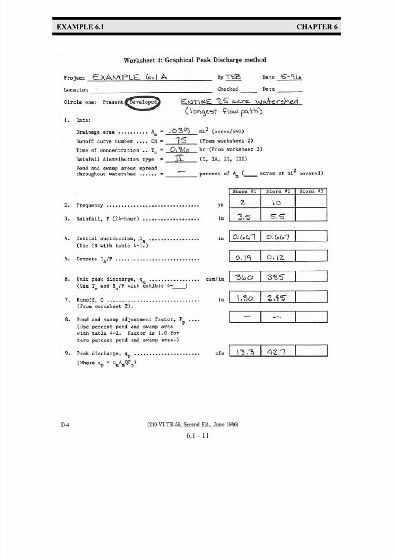
7/30/2019 Virginia Stormwater Managment Handbook Volume_II.pdf
http://slidepdf.com/reader/full/virginia-stormwater-managment-handbook-volumeiipdf 283/354
EXAMPLE 6.1 CHAPTER 6
6.1 - 11
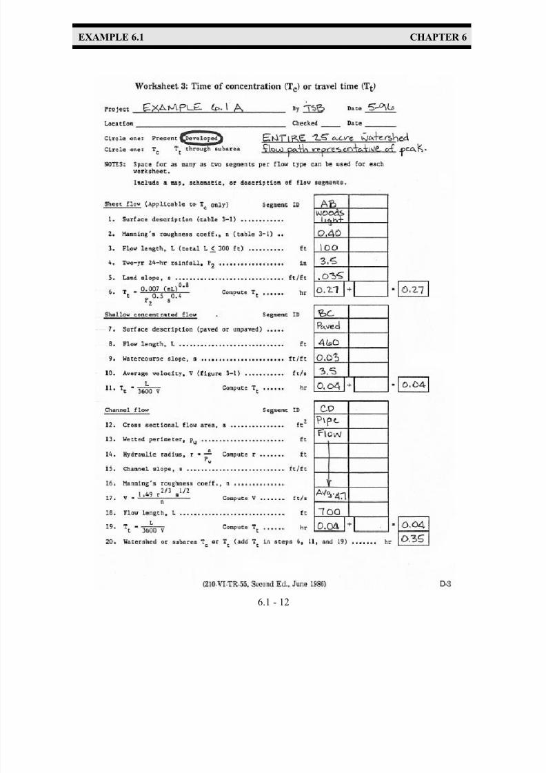
7/30/2019 Virginia Stormwater Managment Handbook Volume_II.pdf
http://slidepdf.com/reader/full/virginia-stormwater-managment-handbook-volumeiipdf 284/354
EXAMPLE 6.1 CHAPTER 6
6.1 - 12

7/30/2019 Virginia Stormwater Managment Handbook Volume_II.pdf
http://slidepdf.com/reader/full/virginia-stormwater-managment-handbook-volumeiipdf 285/354
EXAMPLE 6.1 CHAPTER 6
6.1 - 13

7/30/2019 Virginia Stormwater Managment Handbook Volume_II.pdf
http://slidepdf.com/reader/full/virginia-stormwater-managment-handbook-volumeiipdf 286/354
EXAMPLE 6.1 CHAPTER 6
6.1 - 14

7/30/2019 Virginia Stormwater Managment Handbook Volume_II.pdf
http://slidepdf.com/reader/full/virginia-stormwater-managment-handbook-volumeiipdf 287/354
EXAMPLE 6.1 CHAPTER 6
6.1 - 15
9.38
25.0' 0.38
EXAMPLE 6.1B
The Rational Method can be applied to any given watershed to find the peak discharge at a desired
study point. As discussed inChapter 4, the Rational Method is most accurate for watersheds having
drainage areas of 20 acres or less and t c flow paths of 20 minutes or less. The watershed in this
example will be analyzed using the Rational Method, although it exceeds these limits, to provide a
comparison to the SCS Methods of Part A. The decision to use a particular method is based on the
watershed conditions (size, type of land cover, etc.) and the desired output (the peak rate of runoff,
or a runoff hydrograph). For further discussion of the various methods, see Chapter 4.
Given:
The watershed in Part A of this example, as presented in Figure 6.1-1a,c.
Find:
The pre- and post-developed peak discharge using the Rational Method and the post-developed time
of concentration flow path as described in Part A of this example.
Solution:
The rational method is applied to the 25-acre watershed as follows:
Pre-developed weighted runoff coefficient C:
Land UseArea A
(ac.)
Runoff Coefficient
C C x A
Agriculture 6.25 0.6 3.75
Woods 18.75 0.3 5.63
TOTAL 25.0 9.38
Weighted runoff coefficient C =

7/30/2019 Virginia Stormwater Managment Handbook Volume_II.pdf
http://slidepdf.com/reader/full/virginia-stormwater-managment-handbook-volumeiipdf 288/354
EXAMPLE 6.1 CHAPTER 6
6.1 - 16
14.64
25.0' 0.59
Post-developed weighted runoff coefficient C:
Land Use
Area A
(ac.)
Runoff Coefficient
C C x A
Industrial/
Commercial11.9 0.9 10.71
Woods 13.1 0.3 3.93
TOTAL 25.0 14.64
Weighted runoff coefficient C =
TABLE 6.1 - 2
Hydrologic Summary - Ful l Watershed, Example 6.1B
Rational M ethod Peak Discharge, Q=CIA
Condition
Area
A
(ac.)
Runoff
Coefficient
C
t c *
(min .)
I * *
(in/hr )
Q 2 * * *
(cfs )Q 10 * * *
(cfs )
Pre-developed 25.0 0.3852
.87 hr.
I 2 = 1.8
I 10 = 2.517 24
Post-developed 25.0 0.5921
.35 hr.
I 2 = 3.3
I 10 = 4.449 65
* t c based on SCS methods, Part A
** Intensity from Richmond area IDF curve
*** Rational Method equation: Q=CIA
Comparing these results with those using SCS methods for the same watershed [Table 6.1-1, Post
Developed tc Path (b)], the Rational Method gives a significant increase in the 2-year pre- and post-
developed peak discharges but gives similar discharges for the 10-year storm.

7/30/2019 Virginia Stormwater Managment Handbook Volume_II.pdf
http://slidepdf.com/reader/full/virginia-stormwater-managment-handbook-volumeiipdf 289/354
EXAMPLE 6.1 CHAPTER 6
6.1 - 17
EXAMPLE 6.1C
Example 6.1C divides the given 25-acre watershed into two sub-watersheds. The TR-55 Tabular
Method is used to generate their hydrographs, which are then added at the study point.
Given:
The proposed development disturbs 11.9 acres. Ten acres drain through subwatershed 1 and 1.9
acres drain through subwatershed 2.
Find:
The peak discharge from the watershed by adding the runoff hydrographs from the two sub-
watersheds at the study point.
Solution:
The 25-acre watershed is divided into Sub-watersheds 1 and 2 based on pre- and post-developed land
uses and drainage divides, as shown in Figure 6.1-2. To obtain the peak discharge from the total
watershed, hydrographs must be generated for each sub-watershed and then added at the study point.
The SCS Tabular Method (or any other hydrologic computer program that generates a runoff
hydrograph) should be used.
The results, using the SCS TR-55 Tabular Hydrograph Method, are summarized in Table 6.1-3.
Completed TR-55 worksheets are included at the end of this example.
Referring to the TR-55 Tabular Method Worksheets, note that the peak discharge obtained from
adding the two hydrographs is less than the sum of their individual peaks. This is due to the timing
effect of the peak flow through the watershed. Sometimes, the peak discharge will decrease with
development because of the decreased flow time. Also note that the peak discharge hydrograph for
the developed area travels through the study point before discharge from the other subwatershed(s).
For additional examples and discussion on the Tabular Method, refer to TR-55.
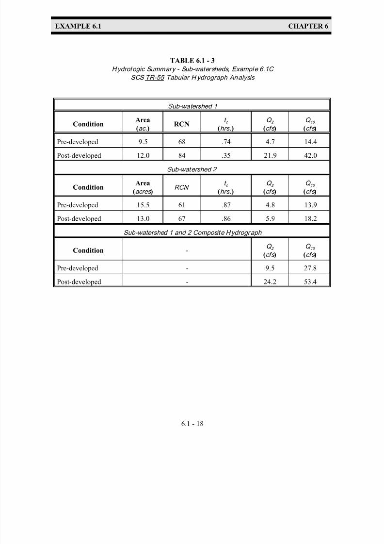
7/30/2019 Virginia Stormwater Managment Handbook Volume_II.pdf
http://slidepdf.com/reader/full/virginia-stormwater-managment-handbook-volumeiipdf 290/354
EXAMPLE 6.1 CHAPTER 6
6.1 - 18
TABLE 6.1 - 3
Hydrologic Summary - Sub-watersheds, Example 6.1C
SCS TR-55 Tabular H ydrograph Analysis
Sub-watershed 1
ConditionArea
(ac.)RCN
t c (hrs.)
Q 2 (cfs )
Q 10 (cfs )
Pre-developed 9.5 68 .74 4.7 14.4
Post-developed 12.0 84 .35 21.9 42.0
Sub-watershed 2
ConditionArea
(acres )RCN
t c (hrs.)
Q 2 (cfs )
Q 10 (cfs )
Pre-developed 15.5 61 .87 4.8 13.9
Post-developed 13.0 67 .86 5.9 18.2
Sub-watershed 1 and 2 Composite Hydrograph
Condition -Q 2
(cfs )
Q 10 (cfs )
Pre-developed - 9.5 27.8
Post-developed - 24.2 53.4

7/30/2019 Virginia Stormwater Managment Handbook Volume_II.pdf
http://slidepdf.com/reader/full/virginia-stormwater-managment-handbook-volumeiipdf 291/354
EXAMPLE 6.1 CHAPTER 6
6.1 - 19
FIGURE 6.1-2a
Example 6.1C Sub-watersheds 1 & 2 Pre-developed Condi tion

7/30/2019 Virginia Stormwater Managment Handbook Volume_II.pdf
http://slidepdf.com/reader/full/virginia-stormwater-managment-handbook-volumeiipdf 292/354
EXAMPLE 6.1 CHAPTER 6
6.1 - 20
FIGURE 6.1-2b
Example 6.1C Sub-watersheds 1 & 2 Post-developed Condi tion

7/30/2019 Virginia Stormwater Managment Handbook Volume_II.pdf
http://slidepdf.com/reader/full/virginia-stormwater-managment-handbook-volumeiipdf 293/354
EXAMPLE 6.1 CHAPTER 6
6.1 - 21

7/30/2019 Virginia Stormwater Managment Handbook Volume_II.pdf
http://slidepdf.com/reader/full/virginia-stormwater-managment-handbook-volumeiipdf 294/354
EXAMPLE 6.1 CHAPTER 6
6.1 - 22

7/30/2019 Virginia Stormwater Managment Handbook Volume_II.pdf
http://slidepdf.com/reader/full/virginia-stormwater-managment-handbook-volumeiipdf 295/354
EXAMPLE 6.1 CHAPTER 6
6.1 - 23
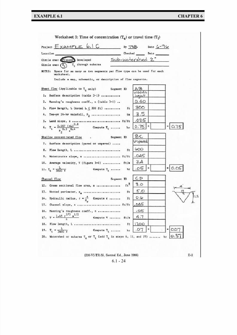
7/30/2019 Virginia Stormwater Managment Handbook Volume_II.pdf
http://slidepdf.com/reader/full/virginia-stormwater-managment-handbook-volumeiipdf 296/354
EXAMPLE 6.1 CHAPTER 6
6.1 - 24

7/30/2019 Virginia Stormwater Managment Handbook Volume_II.pdf
http://slidepdf.com/reader/full/virginia-stormwater-managment-handbook-volumeiipdf 297/354
EXAMPLE 6.1 CHAPTER 6
6.1 - 25

7/30/2019 Virginia Stormwater Managment Handbook Volume_II.pdf
http://slidepdf.com/reader/full/virginia-stormwater-managment-handbook-volumeiipdf 298/354
EXAMPLE 6.1 CHAPTER 6
6.1 - 26
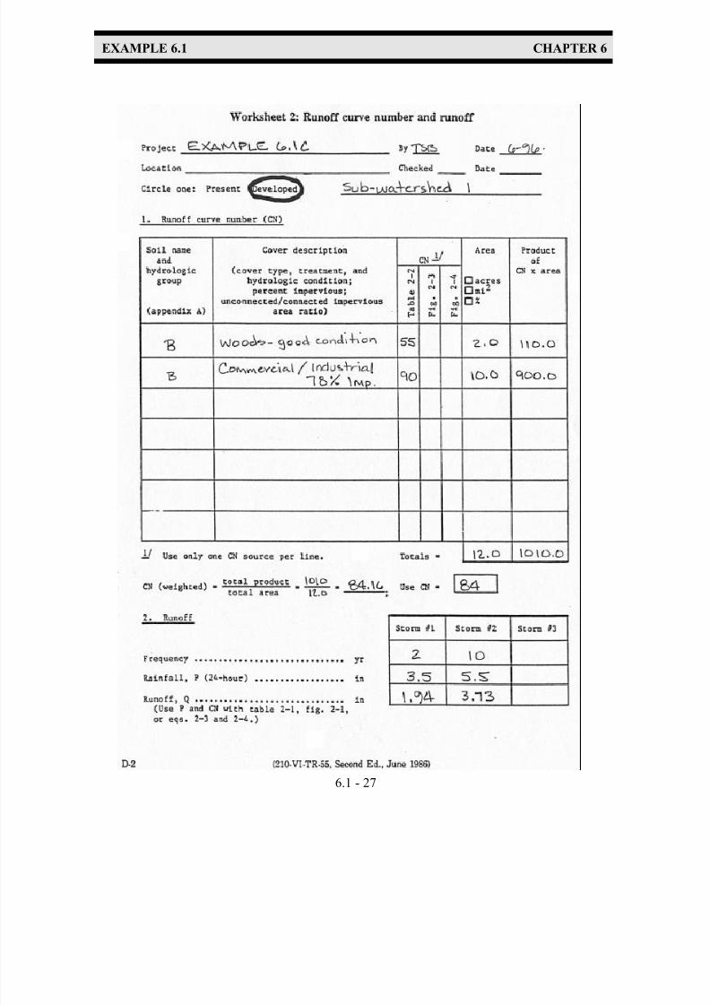
7/30/2019 Virginia Stormwater Managment Handbook Volume_II.pdf
http://slidepdf.com/reader/full/virginia-stormwater-managment-handbook-volumeiipdf 299/354
EXAMPLE 6.1 CHAPTER 6
6.1 - 27
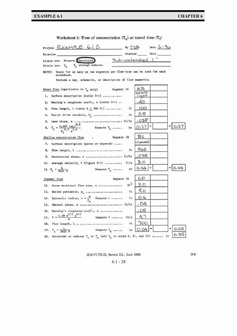
7/30/2019 Virginia Stormwater Managment Handbook Volume_II.pdf
http://slidepdf.com/reader/full/virginia-stormwater-managment-handbook-volumeiipdf 300/354
EXAMPLE 6.1 CHAPTER 6
6.1 - 28
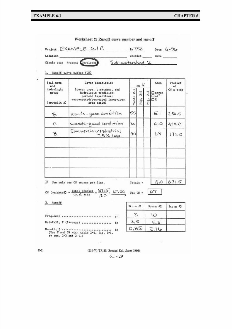
7/30/2019 Virginia Stormwater Managment Handbook Volume_II.pdf
http://slidepdf.com/reader/full/virginia-stormwater-managment-handbook-volumeiipdf 301/354
EXAMPLE 6.1 CHAPTER 6
6.1 - 29
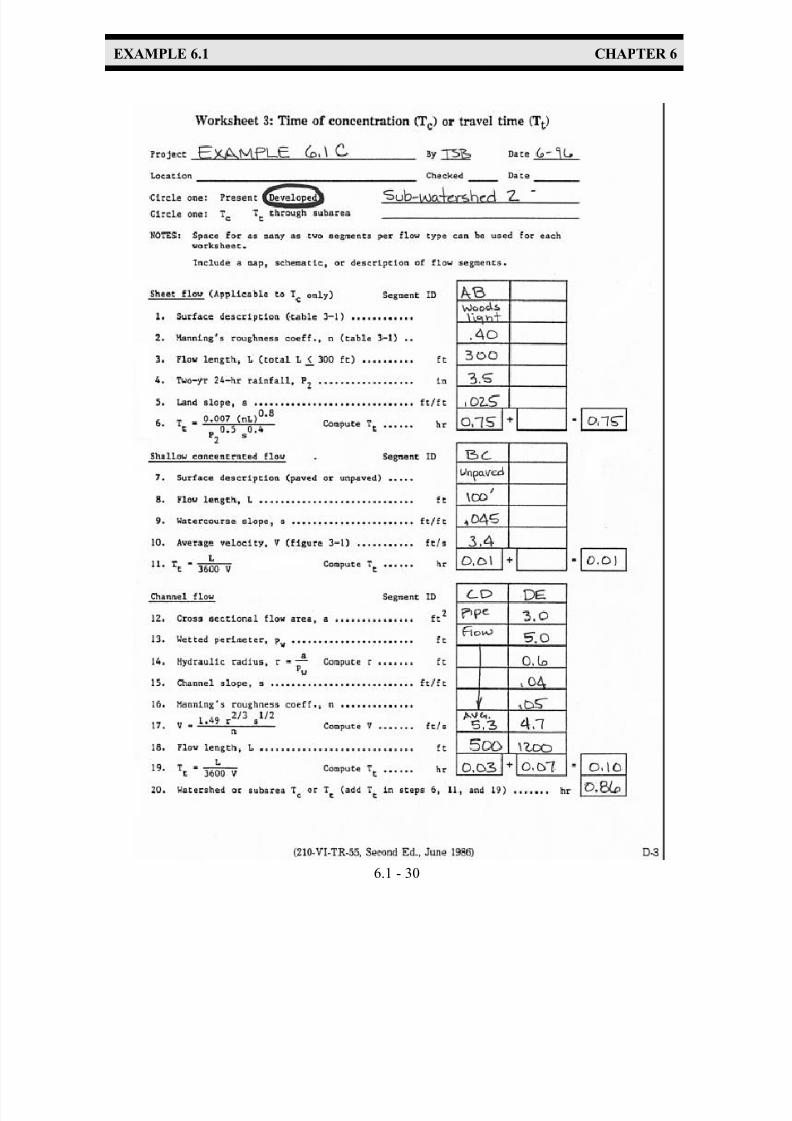
7/30/2019 Virginia Stormwater Managment Handbook Volume_II.pdf
http://slidepdf.com/reader/full/virginia-stormwater-managment-handbook-volumeiipdf 302/354
EXAMPLE 6.1 CHAPTER 6
6.1 - 30

7/30/2019 Virginia Stormwater Managment Handbook Volume_II.pdf
http://slidepdf.com/reader/full/virginia-stormwater-managment-handbook-volumeiipdf 303/354
EXAMPLE 6.1 CHAPTER 6
6.1 - 31
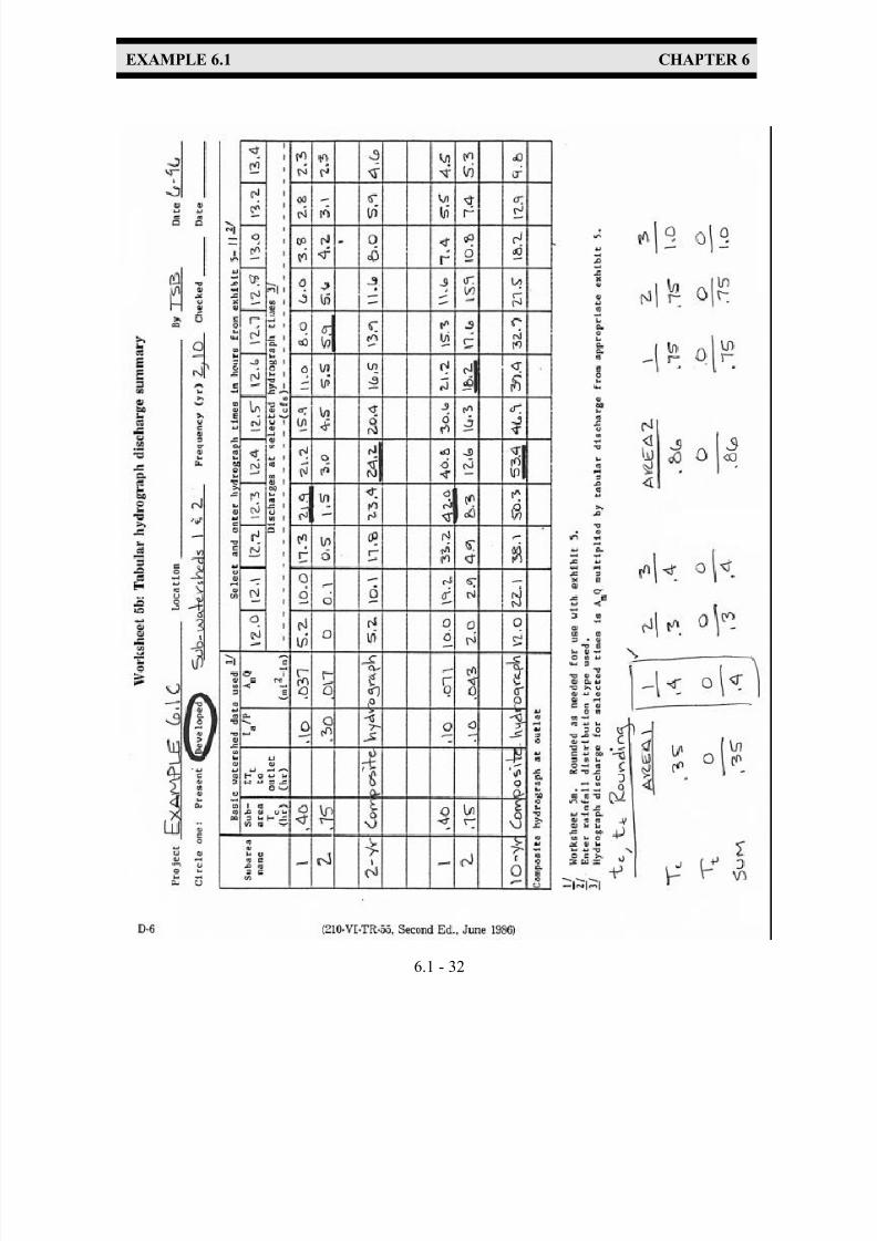
7/30/2019 Virginia Stormwater Managment Handbook Volume_II.pdf
http://slidepdf.com/reader/full/virginia-stormwater-managment-handbook-volumeiipdf 304/354
EXAMPLE 6.1 CHAPTER 6
6.1 - 32
7/30/2019 Virginia Stormwater Managment Handbook Volume_II.pdf
http://slidepdf.com/reader/full/virginia-stormwater-managment-handbook-volumeiipdf 305/354
EXAMPLE 6.1 CHAPTER 6
6.1 - 33
4.56
9.5' 0.48
EXAMPLE 6.1D
Using the Rational Method to analyze the full 25-acre watershed (Example 6.1B) yielded much
higher peak discharges for the 2-year design storm then when using the Tabular Method in Part C.
The analysis of Sub-watershed 1 using the Rational Method will provide a better opportunity to
compare the two methods, since Sub-watershed 1 is less than the recommended maximum of 20 acres
and the tc is close to the recommended 20 minute upper limit.
Given:
Sub-watershed 1 as shown in Figure 6.1-2 and described in Part A.
Find:
The peak discharge from Sub-watershed 1 using the Rational Method. Compare these results withthose from Part C.
Solution:
The Rational Method is applied to Sub-watershed 1 as follows:
Sub-watershed 1:
Pre-developed weighted runoff coefficient C:
Land UseArea A
(ac.)
Runoff Coefficient
C C x A
Agriculture 6.25 0.6 3.75
Woods 3.25 0.25 0.81
TOTAL 9.5 4.56
Weighted runoff coefficient C =

7/30/2019 Virginia Stormwater Managment Handbook Volume_II.pdf
http://slidepdf.com/reader/full/virginia-stormwater-managment-handbook-volumeiipdf 306/354
EXAMPLE 6.1 CHAPTER 6
6.1 - 34
9.5
12.0' 0.79
Post-developed weighted runoff coefficient C:
Land UseArea A
(ac.) Runoff Coefficient
C C x A
Commercial/
Industrial10.0 0.9 9.0
Woods 2.0 0.25 0.5
TOTAL 12.0 9.5
Weighted runoff coefficient =
TABLE 6.1 - 4
Hydrologic Summary - Sub-watershed 1, Example 6.1D
Rational Method Peak Di scharge, Q = CIA
Condition
Area
A
(ac.)
Runoff
Coefficient
C
t c *
(min .)
I * * (in/hr )
Q2
(cfs )
Q10
(cfs )
Pre-developed 9.5 0.48 43.2 I 2 = 2.0;
I 10 = 2.89.1 12.8
Post-developed 12.0 0.79 21
I 2 = 3.3;
I 10 = 4.4 31.3 41.7
* t c based on SCS methods, Part A
** Intensity from Richmond area I-D-F Curve, Appendix 4D
The results show a significant increase in both the pre- and post-developed 2-year storm peak
discharges, and very similar pre- and post-developed 10-year storm peak discharges. This may be
attributed to any one of several factors, however, there seems to be a consistent trend that the
Rational Method over estimates the 2-year storm discharge when compared to the SCS methods.

7/30/2019 Virginia Stormwater Managment Handbook Volume_II.pdf
http://slidepdf.com/reader/full/virginia-stormwater-managment-handbook-volumeiipdf 307/354
Example 6.2
HYDRAULICS
7/30/2019 Virginia Stormwater Managment Handbook Volume_II.pdf
http://slidepdf.com/reader/full/virginia-stormwater-managment-handbook-volumeiipdf 308/354
EXAMPLE 6.2 CHAPTER 6
EXAMPLE 6.2
ILLUSTRATIONS
# FIGURES PAGE
6.2-1 Stage - Storage Table and Curve . . . . . . . . . . . . . . . . . . . . . . . . . . . . . . . . . 6.2-5
6.2-2 Extended Detention Stage-Storage-Discharge Worksheet . . . . . . . . . . . . . . 6.2-7
6.2-3 TR-20 Input and Tabular Output - 1-yr. Extended Detention . . . . . . . . . . . 6.2-8
6.2-4 Extended Detention and 10-year Flood Control (TRIAL 1)Stage-Storage-Discharge Worksheet . . . . . . . . . . . . . . . . . . . . . . . . . . . . . . 6.2-10
6.2-5 TR-20 Input and Output Summary - 1-yr. Extended Detention and
10-yr. Flood Control (TRIAL 1) . . . . . . . . . . . . . . . . . . . . . . . . . . . . . . . . . 6.2-11
6.2-6 Extended Detention and 10-year Flood Control (TRIAL 2)
Stage-Storage-Discharge Worksheet . . . . . . . . . . . . . . . . . . . . . . . . . . . . . . 6.2-13
6.2-7 TR-20 Input and Output Summary - 1-yr. Extended Detention and
10-yr. Flood Control (TRIAL 2) . . . . . . . . . . . . . . . . . . . . . . . . . . . . . . . . . 6.2-14
6.2-8 Stage-Storage-Discharge Table . . . . . . . . . . . . . . . . . . . . . . . . . . . . . . . . . . 6.2-19
6.2-9 TR-20 Input and Output Summary - 1-yr. Extended Detention,
10-yr. Flood Control, 100-yr. Emergency Spillway . . . . . . . . . . . . . . . . . . 6.2-20
6.2-10 Riser Weir and Trash Rack - Perspective . . . . . . . . . . . . . . . . . . . . . . . . . . 6.2-22
6.2-11 Riser Detail - Section . . . . . . . . . . . . . . . . . . . . . . . . . . . . . . . . . . . . . . . . . . 6.2-23
6.2-12 Principal Spillway - Profile . . . . . . . . . . . . . . . . . . . . . . . . . . . . . . . . . . . . . 6.2-24
# TABLES PAGE
6.2-1 Hydrologic Summary Example 6.1, SCS Methods . . . . . . . . . . . . . . . . . . . . 6.2-2

7/30/2019 Virginia Stormwater Managment Handbook Volume_II.pdf
http://slidepdf.com/reader/full/virginia-stormwater-managment-handbook-volumeiipdf 309/354
EXAMPLE 6.2 CHAPTER 6
6.2 - 1
EXAMPLE 6.2
INTRODUCTION:
Example 6.2 will use the same hydrology for the 25-acre watershed that was presented in Example
6.1 and illustrated in Chapter 5. A stormwater facility will be sized and designed to accept the
runoff from the full 25-acre watershed. Note that it is usually most efficient to control stormwater
quality and quantity within the subwatershed where the majority of the development occurs.
GIVEN:
The hydrology of the 25-acre watershed represented in Example 6.1, Part A, using the most
representative flow path of the proposed development to determine the time of concentration. The
summary of the hydrology (developed using the TR-20 computer program) is as follows:
Table 6.2-1
Hydrologic Summary, Example 6.1, SCS Methods
TR-20 COMPUTER RUN
Condition DA RCN t c Q10 Q100
PRE-DEV 25 ac. 64 0.87 hr. 25.5 cfs* 52.7 cfs
POST-DEV 25 ac. 75 0.35 hr. 61.1 cfs 108.9 cfs
* 10-year Allowable release rate
The TR-20 hydrologic analysis input file and output summary are provided on the following pages.
FIND:
Design a stormwater management facility which provides 24 hour extended detention of the 1-year
frequency design storm for channel erosion control, attenuation of the post-developed 10-year
frequency design storm released at the pre-developed rate for flood control, and safe passage of the100-year frequency design storm through a vegetated emergency spillway.
Note: There is no water quality enhancement required for this example. Also, extended detention
of the runoff from the 1-year frequency storm is a calculation based on the volume of runoff
rather than the rate of runoff. Therefore the hydrologic summary includes only the 10- and
100-year frequency storm peak rates of runoff.

7/30/2019 Virginia Stormwater Managment Handbook Volume_II.pdf
http://slidepdf.com/reader/full/virginia-stormwater-managment-handbook-volumeiipdf 310/354
EXAMPLE 6.2 CHAPTER 6
6.2 - 2

7/30/2019 Virginia Stormwater Managment Handbook Volume_II.pdf
http://slidepdf.com/reader/full/virginia-stormwater-managment-handbook-volumeiipdf 311/354
EXAMPLE 6.2 CHAPTER 6
6.2 - 3
V s10 / V r 10
'
V r 10'
V s10
'V
s10
V r 10
V r 10
' (0.31) 5.93 ac. ft . ' 1.84 ac. ft .
SOLUTION:
Use the design procedures found in Chapter 5-7 to design the basin and multi-stage riser structure.
This is to include the design of the 1-year storm extended detention orifice in lieu of a 2-year control
orifice. The design procedures for channel erosion extended detention are found in Chapter 5-6.3.
STEP 1 No water quality requirements for this facility.
STEP 2 Allowable release rates from the TR-20 computer run: Q10 allowable = 25.5 cfs
STEP 3 The required storage volume for extended detention of the 1-year storm (Vce):
1-year frequency design storm rainfall = 2.7" (Appendix 4B); 1-year frequency
design storm runoff = 0.8" (Appendix 4C).
Runoff volume (25 ac.) (0.8") (1'/12") = Vce = 1.66 ac.ft.
Note: The routing affect on the extended detention of the 1-year storm results in the
actual use of approximately 60% of the design storage allocated in the basin
(Chapter 5-6.3). Therefore, Vce = (1.66 ac. ft.) (0.6) = 1.0 ac. ft. = 43,560 ft3.
Required storage volume for 10-year flood control (V10):
1. From TR-55: Storage Volume for Detention Basin (Chapter 5-4.2):
= 25.5 / 61.1 = 0.42Qo10
/Qi10
From Figure 5-4: 0.31
2. Runoff volume: Q10 Am 53.33 = (2.85in.)(0.039 mi2)(53.33) = 5.93 ac.ft.
3. Storage volume required:
Note: Approximately 10% should be added to the required storage to account for theextended detention of the l-year storm within the 10-year design pool: (1.84 ac.ft.)
(1.10) = 2.0 ac.ft.
STEP 4 The development of the stage-storage worksheet and curve, Figure 6.2-1, was presented
in Chapter 5-5.1.

7/30/2019 Virginia Stormwater Managment Handbook Volume_II.pdf
http://slidepdf.com/reader/full/virginia-stormwater-managment-handbook-volumeiipdf 312/354
EXAMPLE 6.2 CHAPTER 6
6.2 - 4
Qavg
'43,560 ft 3
(24hr .)(3,600sec./hr .)' 0.5 cfs
a '1.0
0.6 (2)(32.2)(8.0)' 0.073 ft 2 ' π r 2 ' π d 2 /4
d ' 4a
π
' 4(0.073 ft 2 )
π
' .304ft. '
Q ' Ca 2gh
Q ' 0.6(.073) (2)(32.2)(h) ' 0.33(h)½
STEP 5 The extended detention orifice (1-year storm) is designed using the procedure outlined in
Chapter 5-6.3 as follows:
1. Vce = 1.0 ac.ft.
2. Elevation for 1-year hmax = 89.0 (1.0 ac.ft.). hmax = 89 - 81 = 8.0 ft..
3.
Qmax = 2 × Qavg cfs = 2 × 0.5cfs = 1.0 cfs
4. The required orifice area, a, in ft2 is:
a 'Q
C 2 ghmax
Equation 5-7
Rearranged Orifice equation
3.7 in.
5. Route the 1-year storm to establish the 1-year design water surface elevation (wse)
by completing steps 6 and 7.
6. The stage-discharge relationship is as follows:
Equation 5-6
Orifice equation
where h = wse 81.0 ft.
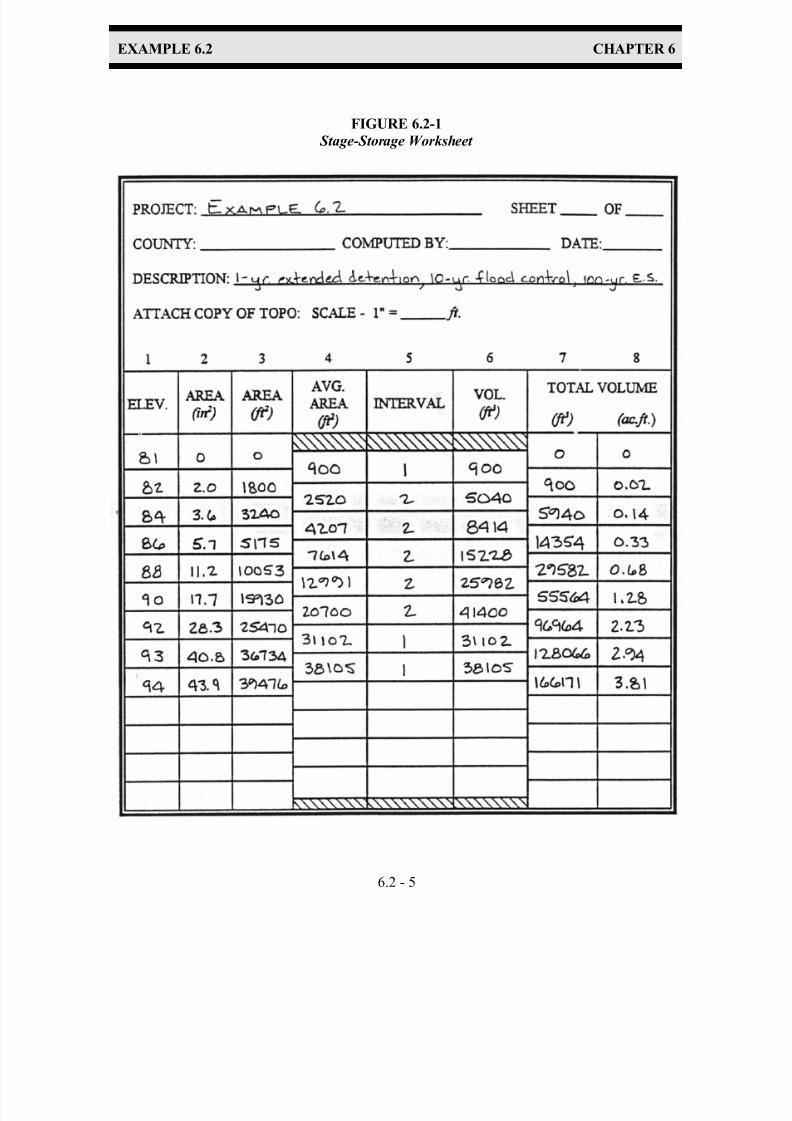
7/30/2019 Virginia Stormwater Managment Handbook Volume_II.pdf
http://slidepdf.com/reader/full/virginia-stormwater-managment-handbook-volumeiipdf 313/354
EXAMPLE 6.2 CHAPTER 6
6.2 - 5
FIGURE 6.2-1
Stage-Storage Worksheet

7/30/2019 Virginia Stormwater Managment Handbook Volume_II.pdf
http://slidepdf.com/reader/full/virginia-stormwater-managment-handbook-volumeiipdf 314/354
EXAMPLE 6.2 CHAPTER 6
6.2 - 6
FIGURE 6.2-1 contd.
Stage - Storage Curve
7. Complete a stage-storage-discharge table for the anticipated range of elevations
using the stage-discharge relationship established in item 6 above. The completed
extended detention portion of the stage-storage-discharge worksheet is presented in
Figure 6.2-2.
In order to establish the 1-year extended detention water surface elevation, the designer may use the
approximate value of 89.0 ft. established by the required storage volume calculation and the stage-
storage curve, or an exact value may be determined by routing the 1-year storm through the basin.
The TR-20 input file and tabular hydrograph output for the routing of the 1-year storm are provided,
Figure 6.2-3. The routing results in a maximum extended detention water surface elevation of
88.69', a peak discharge of 0.97 cfs, and a brim drawdown time of 23.5 hrs. (39 hrs. - 15.5 hrs).
7/30/2019 Virginia Stormwater Managment Handbook Volume_II.pdf
http://slidepdf.com/reader/full/virginia-stormwater-managment-handbook-volumeiipdf 315/354
EXAMPLE 6.2 CHAPTER 6
6.2 - 7
Q = 0.33(h)½ where h = w.s.e. 81.0ft.
FIGURE 6.2-2
Extended Detention Stage-Storage-Discharge Worksheet
STEP 6 / STEP 7 2-year storm control is not required since the channel erosion component of
this design is covered by the extended detention of the 1-year storm.
7/30/2019 Virginia Stormwater Managment Handbook Volume_II.pdf
http://slidepdf.com/reader/full/virginia-stormwater-managment-handbook-volumeiipdf 316/354
EXAMPLE 6.2 CHAPTER 6
6.2 - 8
FIGURE 6.2-3
TR-20 Input and Tabular Output - 1-yr. Extended Detention

7/30/2019 Virginia Stormwater Managment Handbook Volume_II.pdf
http://slidepdf.com/reader/full/virginia-stormwater-managment-handbook-volumeiipdf 317/354
EXAMPLE 6.2 CHAPTER 6
6.2 - 9
STEP 8 (Trial 1) The 10-year flood control opening is designed using the procedures outlined in
Chapter 5-7 as follows:
1. 1-year extended detention water surface elevation is 88.69ft.
2. Set 10-year control elevation at 88.8ft.
3. Approximate storage volume required for 10-year storm control is 2.0 ac.ft. from
STEP 3 above. From the stage storage curve h10max = 91.5ft. 88.8ft. = 2.7ft.
4. The maximum allowable discharge, Q10allowable = 25.5 cfs.
5. A weir is chosen to control the 10-year release rate:
L = Q10allowable / Cwh1.5 Equation 5-9
Rearranged weir equation
L = 25.5 cfs / (3.3) (2.7ft.)1.5
L = 1.74ft. For Trial 1, use a 1ft. - 8in. (1.7ft.) weir
Note: Since the maximum head of 2.7 ft. is used, an average value of 3.3 for the
weir coefficient (Cw) is used. See Table 5-8: Weir Flow Coefficients.
6. The stage discharge relationship is as follows:
Qw = Cw L(h)1. 5 Equation 5-8
Weir flow equation
= 3.3 (1.7ft.) (h)1..5
Qw = 5.6 (h)1. 5 where h = wse 88.8ft.
7. Complete a stage-storage-discharge table for the anticipated range of elevations
using the stage-discharge relationship established in item 6 above. The completed
extended detention and 10-year control (TRIAL 1) portion of the stage-storage-
discharge worksheet is presented in Figure 6.2-4. Note the addition of the
elevation 88.8ft. representing the crest of the 10-year weir.
STEP 9 The TR-20 input file and output summary table for the routing of the 10-year
storm through the basin (Trial 1) are provided (Figure 6.2-5). The routing results
in a 10-year maximum water surface elevation of 91.77ft., and a peak discharge of
29.00 cfs. > 25.5 cfs.
Try smaller weir and repeat from STEP 8, #6.

7/30/2019 Virginia Stormwater Managment Handbook Volume_II.pdf
http://slidepdf.com/reader/full/virginia-stormwater-managment-handbook-volumeiipdf 318/354
EXAMPLE 6.2 CHAPTER 6
6.2 - 10
(1) Q = 0.33(h)1.5 where h = w.s.e. 81.0ft.
(4) Qw = 5.6 (h)1. 5 where h = wse 88.8ft.
FIGURE 6.2-4
Extended Detention and 10-year Flood Control (TRIAL 1) Stage-Storage-Discharge
Worksheet

7/30/2019 Virginia Stormwater Managment Handbook Volume_II.pdf
http://slidepdf.com/reader/full/virginia-stormwater-managment-handbook-volumeiipdf 319/354
EXAMPLE 6.2 CHAPTER 6
6.2 - 11
FIGURE 6.2-5
TR-20 Input and Output Summary - 1-yr. Extended Detention and 10-yr. Flood Control
(TRIAL 1)
7/30/2019 Virginia Stormwater Managment Handbook Volume_II.pdf
http://slidepdf.com/reader/full/virginia-stormwater-managment-handbook-volumeiipdf 320/354
EXAMPLE 6.2 CHAPTER 6
6.2 - 12
STEP 8 6. (Trail 2) Try smaller weir : 1ft. - 4in. (1.33ft.). The stage-discharge relationship
is
as follows:
Qw = Cw L h 1. 5 Equation 5-8
Weir equation
= (3.3) (1.33ft.) (h) 1. 5
Qw = 4.39 (h) 1. 5 where h = wse - 88.8ft.
7. Complete a stage-storage-discharge table for the anticipated range of elevations
using the stage-discharge relationship established in item 6 above. The completed
extended detention and 10-year control (TRIAL 2) portion of the stage-storage-
discharge worksheet is presented in Figure 6.2-6.
STEP 9 The TR-20 input file and output summary table for the routing of the 10-year
storm through the basin (TRIAL 2) are provided (Figure 6.2-7). The routing
results in a maximum water surface elevation of 92.03ft. and a peak discharge of
26.82 cfs. The peak discharge is slightly greater than the allowable, further
reduction may be achieved through the design of the barrel.
7/30/2019 Virginia Stormwater Managment Handbook Volume_II.pdf
http://slidepdf.com/reader/full/virginia-stormwater-managment-handbook-volumeiipdf 321/354
EXAMPLE 6.2 CHAPTER 6
6.2 - 13
(1) Q = 0.33(h)1.5 where h = wse 81.0ft.
(4) Qw = 4.39(h)1. 5 where h = wse 88.8ft
FIGURE 6.2-6
Extended Detention and 10-year Flood Control (TRIAL 2) Stage-Storage-Discharge
Worksheet

7/30/2019 Virginia Stormwater Managment Handbook Volume_II.pdf
http://slidepdf.com/reader/full/virginia-stormwater-managment-handbook-volumeiipdf 322/354
EXAMPLE 6.2 CHAPTER 6
6.2 - 14
FIGURE 6.2-7
TR-20 Input and Output Summary - 1-yr. Extended Detention and 10-yr. Flood Control
(TRIAL 2)
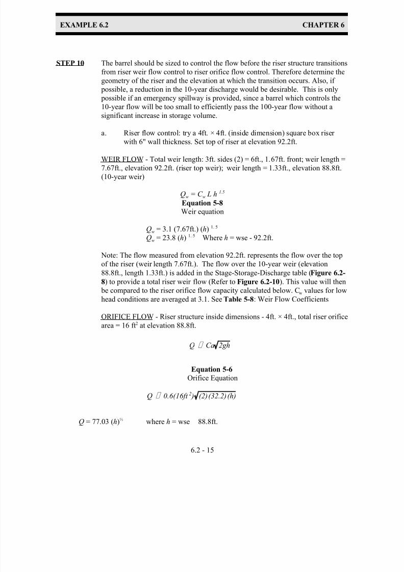
7/30/2019 Virginia Stormwater Managment Handbook Volume_II.pdf
http://slidepdf.com/reader/full/virginia-stormwater-managment-handbook-volumeiipdf 323/354
EXAMPLE 6.2 CHAPTER 6
6.2 - 15
Q ' Ca 2gh
Q ' 0.6(16ft 2 ) (2)(32.2)(h)
STEP 10 The barrel should be sized to control the flow before the riser structure transitions
from riser weir flow control to riser orifice flow control. Therefore determine the
geometry of the riser and the elevation at which the transition occurs. Also, if
possible, a reduction in the 10-year discharge would be desirable. This is only
possible if an emergency spillway is provided, since a barrel which controls the10-year flow will be too small to efficiently pass the 100-year flow without a
significant increase in storage volume.
a. Riser flow control: try a 4ft. × 4ft. (inside dimension) square box riser
with 6" wall thickness. Set top of riser at elevation 92.2ft.
WEIR FLOW - Total weir length: 3ft. sides (2) = 6ft., 1.67ft. front; weir length =
7.67ft., elevation 92.2ft. (riser top weir); weir length = 1.33ft., elevation 88.8ft.
(10-year weir)
Qw = C w L h 1.5
Equation 5-8
Weir equation
Qw = 3.1 (7.67ft.) (h) 1. 5
Qw = 23.8 (h) 1. 5 Where h = wse - 92.2ft.
Note: The flow measured from elevation 92.2ft. represents the flow over the top
of the riser (weir length 7.67ft.). The flow over the 10-year weir (elevation
88.8ft., length 1.33ft.) is added in the Stage-Storage-Discharge table (Figure 6.2-
8) to provide a total riser weir flow (Refer to Figure 6.2-10). This value will then
be compared to the riser orifice flow capacity calculated below. Cw values for low
head conditions are averaged at 3.1. See Table 5-8: Weir Flow Coefficients
ORIFICE FLOW - Riser structure inside dimensions - 4ft. × 4ft., total riser orifice
area = 16 ft2 at elevation 88.8ft.
Equation 5-6
Orifice Equation
Q = 77.03 (h)½ where h = wse 88.8ft.

7/30/2019 Virginia Stormwater Managment Handbook Volume_II.pdf
http://slidepdf.com/reader/full/virginia-stormwater-managment-handbook-volumeiipdf 324/354
EXAMPLE 6.2 CHAPTER 6
6.2 - 16
Q ' Ca 2gh
Q ' 0.6(1.77ft 2 ) (2)(32.2)(h)
Add the riser weir flow and orifice flow values to the stage-storage-discharge table, Figure 6.2-
8.
This analysis shows that the riser does not transition from weir flow to orifice flow
within the range of water surface elevations. Therefore, the barrel does not have to
control the flow. However, we want to slightly restrict the 10-year discharge in order to
reduce it to within 5% of the 10-year allowable release rate.
b. Barrel flow control: upstream invert: 80.75ft., downstream invert: 79.95ft., length
= 80ft.; s = 1.0%
Start with elevation 92ft., determine the HW/D value to be: (92ft. 80.75ft.) / D
= 11.25 / D. To provide the most economical pipe size, or as in this case, to
restrict the flow at approximately 26 cfs in (during the 10-year storm) in order to
achieve better 10-year control, set HW/D = 26 cfs and by trial and error, using
Federal Highway Administration (FHA) culvert nomograph: Figure 5-16
(Headwater Depths for Concrete Pipe Culverts with Inlet Control), entrance
condition 1, determine that an 18 in. pipe comes closest to the desired flow:
HW/D = 11.25 / 1.5 = 7.5 Since the upper limit of the nomograph is HW / D = 6,
use 6, and read Q = 25 cfs. Try 18 in. RCP Barrel.
1. Inlet Control Using the above referenced FHA culvert chart (Figure 5-16)
establish the stage - discharge relationship for an 18 in. concrete pipe barrel, (HW
= wse 80.75), and add these values to the stage-storage-discharge table, Figure
6.2-8.
Where the upper limit of the nomograph HW/D values are exceeded, use the
orifice equation to approximate the inlet control flow values:
Equation 5-6
Orifice Equation
Q = 8.5 (h)½ where h = wse 80.75ft.
2. Outlet Control Use Equation 5-10 to establish the stage-discharge relationship
for the 18" concrete barrel as follows:

7/30/2019 Virginia Stormwater Managment Handbook Volume_II.pdf
http://slidepdf.com/reader/full/virginia-stormwater-managment-handbook-volumeiipdf 325/354
EXAMPLE 6.2 CHAPTER 6
6.2 - 17
Q ' a2gh
1% K m% K p L
Q ' 1.77ft 22(32.2)(h)
1% 1% (.0182)(80ft.)
Equation 5-10
Pipe flow control equation
Where: a = 1.77 ft2
h = wse - (79.95 + D/2) = wse - 80.7
Km = Ke + Kb (from Figure 5-9; square end pipe: Ke =
0.5
= 0.5 + 0.5 = 1.0
Kp = .0182 (from Table 5.10, 18" pipe, ‘n’ = .013
L = 80
Q = 7.64 (h)½ where h = wse 80.75
Add the barrel inlet and outlet control flow values to the stage-storage-discharge
table, Figure 6.2-8.
These flow values indicate the barrel is in outlet control for the entire range of expected
water surface elevations. (The inlet control values are struck out to indicate that the outlet
flow condition controls the discharge). The stage -storage-discharge table indicates that
the barrel controls the discharge at elevation 93ft. and above.
The performance of the 10-year control and barrel hydraulics (Trial 2) can now be checked by
routing the 10-year storm, or the designer may choose to size the emergency spillway first.
STEP 11 The emergency spillway is designed using the procedure outlined in Chapter 5-8 as
follows:
1. 10-year design water surface elevation is 92.03ft. Set the invert of the emergency
spillway at 92.2ft.
2. Q100 = 109 cfs [ 10-year weir release (27 cfs) ] = 82 cfs
3. Since this is a relatively small facility with a low potential downstream hazard in
the case of an embankment failure, the alternate design using Figure 5-23: DesignData for Earth Spillways, is used for the design. We want the maximum stage to
be 93ft. which allows for approximately 0.8ft. (use 1.0ft.) of flow through
spillway. From Figure 5-23: h p = 1.0ft. for a design flow of 81 cfs, read b = 36ft.,
vmax = 4.0ft/s, and smin = 3.0%.
Add these stage-discharge values to the stage-storage-discharge table, Figure 6.2-8.

7/30/2019 Virginia Stormwater Managment Handbook Volume_II.pdf
http://slidepdf.com/reader/full/virginia-stormwater-managment-handbook-volumeiipdf 326/354
EXAMPLE 6.2 CHAPTER 6
6.2 - 18
STEP 12 The TR-20 input file and full output file for the routing of the 1-, 10-, and 100-year
storms through the basin are provided.
STEP 13 Outlet protection is designed using the design procedure presented in Chapter 5-7
(and STD & SPEC 3.18 in the VESCH) as follows:
1. Outlet discharges into a channel with a minimum tailwater condition (Tw < 0.5
barrel diameter).
2. Using Figure 5-20, Q10 = 25.8 cfs and d = 18in., read D50 = 0.8ft. and La = 22ft.
Use Class AI riprap.
3. Riprap apron width is to conform to the existing channel geometry to the top of
bank.
4. The depth of the riprap blanket is 2.25 x 0.9 (Class AI) = 2 ft.
STEP 14 Riser buoyancy calculation (Chapter 5-7) is as follows:
1. Determine buoyant force:
height: 92.2ft. 80.75ft. = 11.45ft. × (4ft.× 4ft.) = 183 ft3;
base: 6ft. × 6ft. × 1ft. = 36 ft3;
total: 219 ft 3 × 62.4 lb/ft3 = 13, 678 lb
2. Downward/resisting force:
volume of riser walls = (11.45ft. × 4ft. × 0.5ft. × 2) + (11.45ft. × 3ft. × 0.5ft. × 2)
= 80.5 ft3;
volume of extended back wall = (1ft. × 4ft. × 0.5ft.) = 2 ft3;
volume of base = (6ft. × 6ft. × 1ft.) = 36 ft3;
volume of 10-year weir cutout = (3.4ft. × 1.33ft. × 0.5ft.) = 2.3 ft3;
volume of 18in. barrel and 10in. ext detention pipe cutouts = (2.41ft2 + 0.78 ft2) ×
0.5ft. = 1.6 ft3;
total downward force = volume of concrete × unit weight (150lb/ft3) : (80.5 ft3 +
2 ft3 + 36 ft3 2.3 ft3 1.6 ft3) × (150lb/ft3) = 17190 lb
3. Safety factor: 13, 678 lb x 1.25 = 17,098 < 17190 lb Riser OK

7/30/2019 Virginia Stormwater Managment Handbook Volume_II.pdf
http://slidepdf.com/reader/full/virginia-stormwater-managment-handbook-volumeiipdf 327/354
EXAMPLE 6.2 CHAPTER 6
6.2 - 19
FIGURE 6.2-8
Stage-Storage-Discharge Table
7/30/2019 Virginia Stormwater Managment Handbook Volume_II.pdf
http://slidepdf.com/reader/full/virginia-stormwater-managment-handbook-volumeiipdf 328/354
EXAMPLE 6.2 CHAPTER 6
6.2 - 20
FIGURE 6.2-9
TR-20 Input and Output Summary - 1-yr. Extended Detention, 10-yr. Flood Control, 100-yr.
Emergency Spillway
7/30/2019 Virginia Stormwater Managment Handbook Volume_II.pdf
http://slidepdf.com/reader/full/virginia-stormwater-managment-handbook-volumeiipdf 329/354
EXAMPLE 6.2 CHAPTER 6
6.2 - 21
S
L s = Y (Z + 4) ˆ 1 + ˆ 0.25 - S
.01
L s = 11.2( 3 + 4 ) ˆ 1 +ˆ 0.25 - .01
STEP 15 Anti-seep collars, rather than a drainage blanket, will be used on this facility since
it is a dry facility. Anti-seep collars are designed using the procedure outlined in
Chapter 5-7 as follows:
1. Length of barrel within saturated zone:
Equation 5-11
Barrel Length in Saturated Zone
where: Y = 92.13ft. 81.0ft. = 11.2ft.
Z = 3H : 1V; = 3
S = 1.0%
L s = 81ft.
OR
Extend a line at 4H:IV from the 10-year water surface elevation at the upstream face of
the embankment downward until it intersects the barrel. The resulting point on the barrel
measures approximately 81ft. From the low flow headwall.
2. (Ls) (0.15) = (81ft.) (0.15) = 12.1ft.
3. For an 18in. (1.5ft.) diameter barrel: 4ft. + 1.5ft. = 5.5ft.
4. Projection = 4ft.
5. Number of collars = 12.1 / 4 = 3 collars. Only two collars are desired: use
a 6ft. projection 6ft. + 1.5ft. = 7.5ft. collars. 12.1 / 6 = 2. Use 2 - 7.5ft.
collars

7/30/2019 Virginia Stormwater Managment Handbook Volume_II.pdf
http://slidepdf.com/reader/full/virginia-stormwater-managment-handbook-volumeiipdf 330/354
EXAMPLE 6.2 CHAPTER 6
6.2 - 22
FIGURE 6.2-10
Riser Weir and Trash Rack - Perspective
7/30/2019 Virginia Stormwater Managment Handbook Volume_II.pdf
http://slidepdf.com/reader/full/virginia-stormwater-managment-handbook-volumeiipdf 331/354
EXAMPLE 6.2 CHAPTER 6
6.2 - 23
FIGURE 6.2-11
Riser Detail - Section
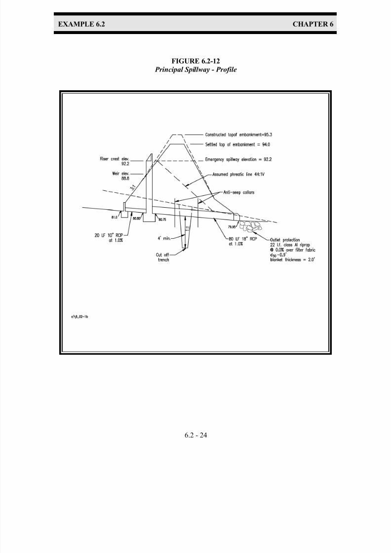
7/30/2019 Virginia Stormwater Managment Handbook Volume_II.pdf
http://slidepdf.com/reader/full/virginia-stormwater-managment-handbook-volumeiipdf 332/354
EXAMPLE 6.2 CHAPTER 6
6.2 - 24
FIGURE 6.2-12
Principal Spillway - Profile

7/30/2019 Virginia Stormwater Managment Handbook Volume_II.pdf
http://slidepdf.com/reader/full/virginia-stormwater-managment-handbook-volumeiipdf 333/354
Example 6.3
BMP SELECTION

7/30/2019 Virginia Stormwater Managment Handbook Volume_II.pdf
http://slidepdf.com/reader/full/virginia-stormwater-managment-handbook-volumeiipdf 334/354
EXAMPLE 6.3 CHAPTER 6
6.3 - 1
EXAMPLE 6.3
INTRODUCTION:
A 90.2 acre site is to be developed into an office park. Perimeter portions of the site are composed
of steep slopes adjacent to two small tributaries which bound the site. Local zoning and Resource
Protection Ordinances restrict the development to the upper, relatively flat center of the property.
(This restriction is does not necessarily limit the development since the engineering costs of
developing on the steep slopes, as well as minimizing the environmental impacts, would be
prohibitive.) The site consists of soils with a moderately high runoff potential (Hydrologic Soil
Group C) with no existing impervious cover.
The proposed buildings, parking lots, and other infrastructure are located on the site such that the
developed condition is drained by three outfalls. These outfalls drain into the adjacent stream
channels at the naturally occurring drainage paths from the site. The local stormwater management
(SWM) program requires that all three components of stormwater management, water quality,
stream channel erosion, and flooding, be investigated. This example will illustrate the application
of these components, including a discussion of the Performance-based and Technology-based water
quality criteria.
GIVEN:
The pre- and post-developed hydrology for the site is presented in Table 6-3.1. The drainage areas
are measured to the proposed study points which have been located at the downstream limit of the
potential BMP locations.
FIND:
Evaluate the BMP options and select the combination which best serve the proposed development.
SOLUTION:
The implementation of stormwater BMPs should be considered during the initial stages of the site
design. An evaluation of the stormwater requirements prior to site design will allow the engineer to
identify potential BMP locations and provide the most efficient alignment of the drainage
infrastructure so as to enhance the use of natural drainage ways to convey stormwater runoff. (The
internal drainage systems must satisfy the Erosion and Sediment Control, MS-19 criteria for channel
adequacy.) Once the preliminary site design is completed, the engineer can calculate the water
quality volume, pollutant loadings, peak rates of discharge, and channel capacities in order to
finalize the BMP strategy for the site.
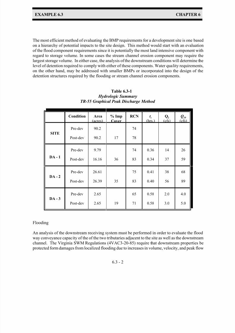
7/30/2019 Virginia Stormwater Managment Handbook Volume_II.pdf
http://slidepdf.com/reader/full/virginia-stormwater-managment-handbook-volumeiipdf 335/354
EXAMPLE 6.3 CHAPTER 6
6.3 - 2
The most efficient method of evaluating the BMP requirements for a development site is one based
on a hierarchy of potential impacts to the site design. This method would start with an evaluation
of the flood component requirements since it is potentially the most land intensive component with
regard to storage volume. In some cases the stream channel erosion component may require thelargest storage volume. In either case, the analysis of the downstream conditions will determine the
level of detention required to comply with either of these components. Water quality requirements,
on the other hand, may be addressed with smaller BMPs or incorporated into the design of the
detention structures required by the flooding or stream channel erosion components.
Table 6.3-1
Hydrologic Summary
TR-55 Graphical Peak Discharge Method
Condition Area
(acres)
% Imp
Cover
RCN t c(hrs.)
Q2
(cfs)
Q10
(cfs)
SITE
Pre-dev
Post-dev
90.2
90.2 17
74
78
DA - 1
Pre-dev
Post-dev
9.79
16.16 36
74
83
0.36
0.34
14
37
26
59
DA - 2
Pre-dev
Post-dev
26.61
26.39 35
75
83
0.41
0.40
38
56
68
89
DA - 3
Pre-dev
Post-dev
2.65
2.65 19
65
71
0.58
0.58
2.0
3.0
4.0
5.0
Flooding
An analysis of the downstream receiving system must be performed in order to evaluate the flood
way conveyance capacity of the of the two tributaries adjacent to the site as well as the downstream
channel. The Virginia SWM Regulations (4VAC3-20-85) require that downstream properties be
protected form damages from localized flooding due to increases in volume, velocity, and peak flow
7/30/2019 Virginia Stormwater Managment Handbook Volume_II.pdf
http://slidepdf.com/reader/full/virginia-stormwater-managment-handbook-volumeiipdf 336/354
EXAMPLE 6.3 CHAPTER 6
6.3 - 3
rate of stormwater runoff by detaining the 10-year post-developed peak rate of runoff and releasing
it at the pre-developed rate. There is also a provision which allows an alternate criteria based upon
geographic, land use, topographic, geologic factors or other downstream conveyance factors as
appropriate. In this case, the local government has a Flodplain Management Ordinance in placewhich has restricted development within the flood way of the tributaries and the downstream
channel. The analysis of the flood way reveals that there is sufficient capacity to convey the ultimate
development condition runoff within the flood way, and that there is no existing development (or
structures) within the flood way for the entire downstream reach to the confluence with the river.
Flood control (10-year storm) is not required in this case.
Stream Channel Erosion
The Virginia SWM Regulations (4VAC3-20-81) require that properties and receiving waterways
downstream of any land development project be protected from erosion and damage due to increasesin volume, velocity, and peak flow rate of stormwater runoff. A rigorous analysis of the downstream
channel is required in order to verify the adequacy for conveying the post-developed runoff. The
following items were completed for each channel in order to adequately verify the analysis:
1. Channel geometry - A minimum of three surveyed cross-sections were taken at a minimum
spacing of 50' along the channel length downstream of the discharge point.
2. Channel lining - A sample of the channel lining was collected and analyzed to determine
the composition relative to the permissible velocities found in Table 5-22 of the Virginia
Erosion and Sediment Control Handbook.
3. Channel slope - Relative elevations were taken along the channel length at the channel cross
sections in order to determine the average longitudinal slope of the channel.
4. Channel Inspection - The channel was physically inspected by walking the length to verify
that there are no significant changes or obstructions such as undersized culverts or other
“improved” restrictions which may restrict the flow and cause it to jump the banks or
increase in velocity to an erosive level.
The channel analysis indicated that the post-developed condition runoff would cause an erosive
condition in specific sections of the channel where the flow area narrows considerably. In addition,
the physical inspection verified that several of these narrow areas as well as several bends arealready experiencing some erosion under existing runoff conditions. Some of the options considered
include:
1. Channel improvements - Channel improvements are is ruled out due to poor access
conditions to the channel. Significant clearing would be required to not only gain access but
also to maneuver construction equipment adjacent to the channels. Some possibilities do
7/30/2019 Virginia Stormwater Managment Handbook Volume_II.pdf
http://slidepdf.com/reader/full/virginia-stormwater-managment-handbook-volumeiipdf 337/354
EXAMPLE 6.3 CHAPTER 6
6.3 - 4
exist for hand placed bioengineering stabilization of the eroded portions of the channel.
2. Alternative site design - Several alternate site configurations were evaluated in an effort to
reduce the impervious cover, disconnect the impervious cover from the drainage system
(disconnecting impervious cover include discharging roof down spouts into dry wells or intosheet flow conditions over pervious areas, placing grass or landscaped buffer strips between
impervious surfaces and the improved drainage structures and conveyances), and create
small pockets in which to detain runoff in an effort to increase the hydrologic flow time and
decrease the peak rate of runoff from the site. While these efforts did result in some
significant reductions in post-developed runoff, the resulting peak rate was still determined
to be too high for the stream channels to convey in a non-erosive manner.
3. Combination of channel improvements, site design, and detention - The hydrologic
analysis of the post-developed condition with the various alternative site designs and 24 hour
extended detention of the runoff from the 1-year frequency storm yielded a peak rate of
runoff significantly less than the runoff from the pre-developed condition 2-year storm.Further analysis indicated that the statistical occurrence frequency of the post-developed
condition peak runoff equivalent to the pre-developed 2-year peak runoff occurs less than
once in 5 years. This means that, according to the statistical analysis, it would take a five
year frequency storm event to generate the pre-developed 2-year peak rate of runoff leaving
the site.
Alternative 3 was selected in order to attempt to stabilize the natural channels adjacent to the site.
Extended detention basins designed to detain the runoff from the 1-year 24 hour storm will be placed
in drainage areas 1 (DA-1) and 2 (DA-2).
Water Quality
The designer must select either the Performance-based or Technology-based water quality criteria.
The technology-based criteria considers the drainage area size and impervious cover draining to a
BMP to establish the best available technology (BMP) for the drainage area or site being evaluated.
The performance-based criteria uses the percent impervious cover of the site to calculate a total site
pre- and post-developed pollutant load. The engineer then implements a BMP strategy which
satisfies the total site pollutant reduction requirement.
Since the Performance-based water quality criteria allows for overall site compliance, it is not
always necessary to place a water quality BMP in each drainage area on the site. DCR recommends,
however, that the engineer evaluate the potential pollutant loading based on the amount of impervious cover and the concentration of that cover. In other words, if the impervious cover is
concentrated, or located such that an improved drainage system is collecting the runoff, then the
implementation of a water quality BMP(s) should be implemented for that area. This is the preferred
solution, rather than placing a BMP in one drainage area, satisfying the performance-based total site
pollutant removal requirement for the site, and then ignoring the other drainage areas and their

7/30/2019 Virginia Stormwater Managment Handbook Volume_II.pdf
http://slidepdf.com/reader/full/virginia-stormwater-managment-handbook-volumeiipdf 338/354
EXAMPLE 6.3 CHAPTER 6
6.3 - 5
A planning area is defined as a designated portion of the parcel on which the land
development project is located. Planning areas shall be established by delineation on a
master plan. Once established, planning areas shall be applied consistently for all future
projects.
associated impacts on downstream water quality. The key to the successful implementation of this
recommendation is a menu of available, cost effective, and low maintenance BMPs. The menu of
BMPs found in Table 1 of the SWM Regulations, as well as the several new and innovative BMPs
currently available, provide several low cost options. This is one of the strategies of Low ImpactDevelopment: relatively small and maintenance free BMPs to control small portions of the
development area in landscaped settings in addition to development strategies which effectively
reduce the impact of the impervious area on the runoff from the site. (Refer to the references found
at the end of Chapter 2 for more information on Low Impact Development.)
This example illustrates a development scenario in which the percent impervious cover
determination for the performance-based criteria plays a significant role in the BMP strategy. The
percent impervious cover for the property is low (15.73 acres of impervious cover on a 90.2 acre
site: 17% impervious cover). The percent impervious cover for the individual drainage areas to the
potential BMP locations, however, is much higher (a total of 45.2 acres at 35% impervious cover).
As discussed in Chapter 2, one of the effects of using impervious cover as a regulatory water quality yardstick is to encourage the minimization of impervious cover and the preservation of green
space and environmentally sensitive areas. In this example, the total impervious cover is limited to
17% of the site.
When using the performance-based criteria the derived benefit of such a low percent impervious
cover is a minimal pollutant removal requirement. This minimal removal requirement illustrates the
discussion above: a BMP placed in one of the drainage areas will most likely satisfy the removal
requirement for the site, and the remaining drainage areas could be left uncontrolled for water
quality. It stands to reason, however, that the highly concentrated impervious cover found within
the other drainage areas will have a significant impact on the water quality of the adjacent streams.
The use of the entire site to determine the percent impervious cover does not accurately reflect thechanges to the land use. Therefore, when using the performance-based criteria for large
development parcels, DCR recommends that the percent impervious cover be calculated by
using the drainage areas or an established planning area. In this example, a planning area
may be established which consists of the portion of the site which is able to be developed.

7/30/2019 Virginia Stormwater Managment Handbook Volume_II.pdf
http://slidepdf.com/reader/full/virginia-stormwater-managment-handbook-volumeiipdf 339/354
EXAMPLE 6.3 CHAPTER 6
6.3 - 6
The water quality requirements in terms of pollutant load removal are calculated using the
Performance-Based Water Quality Calculations: Worksheet 2 provided in Appendix 5D, and
summarized below:
TRIAL 1: Entire site.
STEP 4: Equation 5-16
Lpre(watershed) = [0.05 + (0.009 × 16% )] × 90.2 ac. × 2.28 = 39.9 pounds per year
STEP 5: Equation 5-21
Lpost = [0.05 + (0.009 × 17.4% )] × 90.2 ac. × 2.28 = 42.5 pounds per year
STEP 6:
RR = 42.5 39.9 = 2.6 pounds per year
STEP 7:
EFF = ( 2.6 ÷ 42.5 ) × 100 = 6.1 %
If a BMP could serve the entire site, then a removal efficiency of 6.1% would be required. Since
this can not be done, a minimum of 2.6 pounds of phosphorus must be removed from any one or
combination of the drainage areas of the developed portion of the site.
TRIAL 2: Planning area consisting of the developable area of the site: 45.2 acres
STEP 4: Equation 5-16
Lpre(watershed) = [0.05 + (0.009 × 16% )] × 45.2 ac. × 2.28 = 20.0 pounds per year
STEP 5: Equation 5-21
Lpost = [0.05 + (0.009 × 35.0% )] × 45.2 ac. × 2.28 = 37.6 pounds per year
STEP 6:
RR = 37.6 20.0 = 17.6 pounds per year
STEP 7:
(1.) EFF = ( 17.6 ÷ 37.6 ) × 100 = 46.8 %
When considering the whole site (90.2 acres at 17% impervious cover), the pollutant removal
requirement is 6% of the post-developed load (or 2.6 lbs of phosphorus) as calculated in Trial 1.
When just the drainage areas to the BMP locations are considered (45.2 acres at 35% impervious
cover), the pollutant removal requirement is 46.8% of the post-developed load (or 17.6 lbs of
phosphorus).
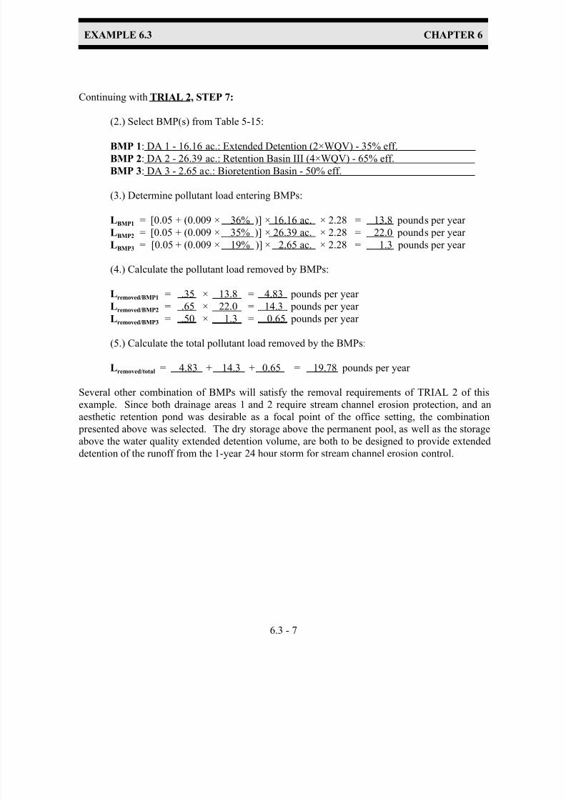
7/30/2019 Virginia Stormwater Managment Handbook Volume_II.pdf
http://slidepdf.com/reader/full/virginia-stormwater-managment-handbook-volumeiipdf 340/354
EXAMPLE 6.3 CHAPTER 6
6.3 - 7
Continuing with TRIAL 2, STEP 7:
(2.) Select BMP(s) from Table 5-15:
BMP 1: DA 1 - 16.16 ac.: Extended Detention (2×WQV) - 35% eff.
BMP 2: DA 2 - 26.39 ac.: Retention Basin III (4×WQV) - 65% eff.
BMP 3: DA 3 - 2.65 ac.: Bioretention Basin - 50% eff.
(3.) Determine pollutant load entering BMPs:
LBMP1 = [0.05 + (0.009 × 36% )] × 16.16 ac. × 2.28 = 13.8 pounds per year
LBMP2 = [0.05 + (0.009 × 35% )] × 26.39 ac. × 2.28 = 22.0 pounds per year
LBMP3 = [0.05 + (0.009 × 19% )] × 2.65 ac. × 2.28 = 1.3 pounds per year
(4.) Calculate the pollutant load removed by BMPs:
Lremoved/BMP1 = .35 × 13.8 = 4.83 pounds per year
Lremoved/BMP2 = .65 × 22.0 = 14.3 pounds per year
Lremoved/BMP3 = .50 × 1.3 = 0.65 pounds per year
(5.) Calculate the total pollutant load removed by the BMPs:
Lremoved/total = 4.83 + 14.3 + 0.65 = 19.78 pounds per year
Several other combination of BMPs will satisfy the removal requirements of TRIAL 2 of this
example. Since both drainage areas 1 and 2 require stream channel erosion protection, and anaesthetic retention pond was desirable as a focal point of the office setting, the combination
presented above was selected. The dry storage above the permanent pool, as well as the storage
above the water quality extended detention volume, are both to be designed to provide extended
detention of the runoff from the 1-year 24 hour storm for stream channel erosion control.

7/30/2019 Virginia Stormwater Managment Handbook Volume_II.pdf
http://slidepdf.com/reader/full/virginia-stormwater-managment-handbook-volumeiipdf 341/354
GLOSSARY
7/30/2019 Virginia Stormwater Managment Handbook Volume_II.pdf
http://slidepdf.com/reader/full/virginia-stormwater-managment-handbook-volumeiipdf 342/354
VIRGINIA STORMWATER MANAGEMENT HANDBOOK GLOSSARY
G - 1
Glossary of Stormwater Management Terms and Acronyms
AASHTO - American Association of State and Highway Transportation Officials
Adsorption - The process by which a solute is attracted to a solid surface. Adsorption is the process
utilized in stormwater management BMPs to enhance the removal of soluble pollutants.
Anti-seep collar - A device constructed around a pipe or other conduit and placed into a dam, levee,
or dike for the purpose of reducing seepage losses and piping failures along the conduit it surrounds.
Anti-vortex device - A device placed at the entrance to a pipe conduit structure to help prevent
swirling action and cavitation from reducing the flow capacity of the conduit system.
Aquatic bench - A 10- to 15-foot wide bench around the inside perimeter of a permanent pool that
ranges in depth from zero to 12 inches. Vegetated with emergent plants, the bench augments pollutant removal, provides habitats, protects the shoreline from the effects of water level
fluctuations, and enhances safety.
Aquifer - A porous, water bearing geologic formation generally restricted to materials capable of
yielding an appreciable supply of water.
As-built (drawing) - Drawing or certification of conditions as they were actually constructed.
Atmospheric Deposition - The process by which atmospheric pollutants reach the land surface either
as dry deposition or as dissolved or particulate matter contained in precipitation.
Average land cover condition - The percentage of impervious cover considered to generate an
equivalent amount of phosphorus as the total combined land uses within the Chesapeake Bay
watershed at the time of the Chesapeake Bay Preservation Act adoption, assumed to be 16%. Note
that a locality may opt to calculate actual watershed specific values for the average land cover
condition based upon 4VAC 3-20-101.
Baffle - Guides, grids, grating or similar devices placed in a pond to deflect or regulate flow and
create a longer flow path from the inlet to the outlet structure.
Bankfull flow - Condition where flow fills a stream channel to the top of bank and at a point where
the water begins to overflow onto a floodplain.
Barrel - Closed conduit used to convey water under or through an embankment, part of the principal
spillway.
Base flow - Discharge of water independent of surface runoff conditions, usually a function of
groundwater levels.
7/30/2019 Virginia Stormwater Managment Handbook Volume_II.pdf
http://slidepdf.com/reader/full/virginia-stormwater-managment-handbook-volumeiipdf 343/354
VIRGINIA STORMWATER MANAGEMENT HANDBOOK GLOSSARY
G - 2
Basin - A facility designed to impound stormwater runoff.
Best Management Practice (BMP) - Structural or nonstructural practice which is designed to
minimize the impacts of changes in land use on surface and groundwater systems. Structural BMPrefers to basins or facilities engineered for the purpose of reducing the pollutant load in stormwater
runoff, such as Bioretention, constructed stormwater wetlands, etc. Nonstructural BMP refers to
land use or development practices which are determined to be effective in minimizing the impact
on receiving stream systems, such as preservation of open space and stream buffers, disconnection
of impervious surfaces, etc.
Biochemical Oxygen Demand (BOD) - An indirect measure of the concentration of biologically
degradable material present in organic wastes. It usually reflects the amount of oxygen consumed
in five days by biological processes breaking down organic waste.
Biological Processes - A pollutant removal pathway in which microbes break down organic pollutants and transform nutrients.
Bioretention basin - Water quality BMP engineered to filter the water quality volume through an
engineered planting bed, consisting of a vegetated surface layer (vegetation, mulch, ground cover),
planting soil, and sand bed (optional), and into the in-situ material. Also called rain gardens.
Bioretention filter - A bioretention basin with the addition of a sand layer and collector pipe system
beneath the planting bed.
CBLAD - Chesapeake Bay Local Assistance Department (Virginia state agency).
COE - United States Army Corps of Engineers
Catch Basin - An inlet chamber usually built at the curb line of a street or low area, for collection
of surface runoff and admission into a sewer or subdrain. These structures commonly have a
sediment sump at its base, below the sewer or subdrain discharge elevation, designed to retain solids
below the point of overflow.
Channel - A natural or manmade waterway.
Channel stabilization - The introduction of natural or manmade materials placed within a channel
so as to prevent or minimize the erosion of the channel bed and/or banks.
Check dam - Small dam constructed in a channel for the purpose of decreasing the flow velocity,
minimize channel scour, and promote deposition of sediment. Check dams are a component of
grassed swale BMPs.
Chemical Oxygen Demand (COD) - A measure of the oxygen required to oxidize all compounds,
both organic and inorganic, in water.
7/30/2019 Virginia Stormwater Managment Handbook Volume_II.pdf
http://slidepdf.com/reader/full/virginia-stormwater-managment-handbook-volumeiipdf 344/354
VIRGINIA STORMWATER MANAGEMENT HANDBOOK GLOSSARY
G - 3
Chute - A high velocity, open channel for conveying water to a lower level without erosion.
Compaction - The process by which soil grains are rearranged so as to decrease void space and
bring them in closer contact with one another, thereby reducing the permeability and increasingthe soils unit weight, and shear and bearing strength.
Conduit - Any channel intended for the conveyance of water, whether open or closed.
Constructed stormwater wetlands - Areas intentionally designed and created to emulate the water
quality improvement function of wetlands for the primary purpose of removing pollutants from
stormwater.
Contour - A line representing a specific elevation on the land surface or a map.
Cradle - A structure usually of concrete shaped to fit around the bottom and sides of a conduit to
support the conduit, increase its strength and, in dams, to fill all voids between the underside of theconduit and soil.
Crest - The top of a dam, dike, spillway or weir, frequently restricted to the overflow portion.
Curve number (CN) - A numerical representation of a given area’s hydrologic soil group, plant
cover, impervious cover, interception and surface storage derived in accordance with Natural
Resource Conservation Service methods. This number is used to convert rainfall depth into runoff
volume. Sometimes referred to as Runoff Curve Number.
Cut - A reference to an area or material that has been excavated in the process of a grading
operation.
Dam - A barrier constructed for the purpose of confining or impounding water.
DCR - Virginia Department of Conservation and Recreation.
DEQ - Virginia Department of Environmental Quality.
Design Storm - A selected rainfall heyetograph of specified amount, intensity, duration and
frequency that is used as a basis for design.
Detention - The temporary impoundment or holding of stormwater runoff.
Detention Basin - A stormwater management facility which temporarily impounds runoff and
discharges it through a hydraulic outlet structure to a downstream conveyance system. While a
certain amount of outflow may also occur via infiltration through the surrounding soil, such amounts
are negligible when compared to the outlet structure discharge rates and, therefore, are not
considered in the facility’s design. Since an extended detention basin impounds runoff only
temporarily, it is normally dry during nonrainfall periods. See MS 3.08.

7/30/2019 Virginia Stormwater Managment Handbook Volume_II.pdf
http://slidepdf.com/reader/full/virginia-stormwater-managment-handbook-volumeiipdf 345/354
VIRGINIA STORMWATER MANAGEMENT HANDBOOK GLOSSARY
G - 4
Dike - An embankment, usually linear, to confine or direct water.
Discharge - Flow of water across the land surface or within the confines of a natural or manmade
channel, or stream.
Dissolved Oxygen - A form of oxygen found in water that is essential to the life of aquatic species.
Disturbed area - An area in which the natural vegetative soil cover or existing surface treatment has
been removed or altered and, therefore, is susceptible to erosion.
Diversion - A channel or dike constructed to direct water to areas where it can be used, treated, or
disposed of safely.
Drainage basin - An area of land that contributes stormwater runoff to a designated point. Also
called a drainage area or, on a larger scale, a watershed.
Drop structure - A manmade device constructed to transition water to a lower elevation.
Duration - The length of time over which precipitation occurs.
EPA - The United States Environmental Protection Agency.
Embankment - A man-made deposit of soil, rock or other material used to form an impoundment.
Emergency Spillway - A channel, usually an open channel constructed adjacent to an embankment,
which conveys flows in excess of the design capacity of the principal spillway.
Energy dissipator - A device used to reduce the velocity or turbulence of flowing water.
Erosion - The wearing away of the land surface by running water, wind, ice or other geological
agents.
Accelerated erosion - erosion in excess of what is presumed or estimated to be naturally
occurring levels and which is a direct result of human activities.
Gully erosion - erosion process whereby water accumulates in narrow channels and removes
the soil to depths ranging from a few inches to 1 or 2 feet to as much as 75 to 100 feet.
Rill erosion - erosion process in which numerous small channels only several inches deep
are formed.
Sheet erosion - spattering of small soil particles caused by the impact of raindrops on wet
soils. The loosened and spattered particles may subsequently be removed by surface runoff.

7/30/2019 Virginia Stormwater Managment Handbook Volume_II.pdf
http://slidepdf.com/reader/full/virginia-stormwater-managment-handbook-volumeiipdf 346/354
VIRGINIA STORMWATER MANAGEMENT HANDBOOK GLOSSARY
G - 5
Eutrophication - The process of over-enrichment of water bodies by nutrients often typified by the
presence of algal blooms.
Extended detention basin - A stormwater management facility which temporarily impounds runoff and discharges it through a hydraulic outlet structure over a specified period of time to a downstream
conveyance system for the purpose of water quality enhancement or stream channel erosion control.
While a certain amount of outflow may also occur via infiltration through the surrounding soil, such
amounts are negligible when compared to the outlet structure discharge rates and, therefore, are not
considered in the facility's design. Since an extended detention basin impounds runoff only
temporarily, it is normally dry during nonrainfall periods.
Extended detention basin-enhanced - An extended detention basin modified to increase pollutant
removal by providing a shallow marsh in the lower stage of the basin.
Exfiltration - The downward movement of runoff through the bottom of a stormwater facility andinto the soil.
Fill - A reference to an area or material that has been placed by mechanical equipment in the process
of a grading operation.
Filter bed - The section of a constructed filtration device that houses the filtering media.
Filter Strip - An area of vegetation, usually adjacent to a developed area, constructed to remove
sediment, organic matter, and other pollutants from runoff in the form of sheet flow.
First flush - The first portion of runoff, usually defined as a depth in inches, considered tocontaining the highest pollutant concentration resulting from a rainfall event.
Flooding - When the volume or rate flow exceeds the capacity of the natural or manmade
conveyance system and overflows onto adjacent lands, causing or threatening damage.
Floodplain - For a given flood event, that area of land adjoining a continuous water course which
has been covered temporarily by water.
Flow splitter - An engineered hydraulic structure designed to divert a portion of storm flow to a
BMP located out of the primary channel, or to direct stormwater to a parallel pipe system, or to
bypass a portion of baseflow around a BMP.
Forebay - Storage space, commonly referred to as a sediment forebay, located near a stormwater
BMP inlet that serves to trap incoming coarse sediments before they accumulate in the main
treatment area.
Freeboard - Vertical distance between the surface elevation of the design high water and the top of
a dam, levee, or diversion ridge.

7/30/2019 Virginia Stormwater Managment Handbook Volume_II.pdf
http://slidepdf.com/reader/full/virginia-stormwater-managment-handbook-volumeiipdf 347/354
VIRGINIA STORMWATER MANAGEMENT HANDBOOK GLOSSARY
G - 6
French drain - A type of drain consisting of an excavated trench filled with pervious material such
as coarse sand, gravel or crushed stone, through whose voids water percolates and exfiltrates into
the soil.
Frequency (design storm frequency) - The recurrence interval of storm events having the same
duration and volume. The frequency of a specified design storm can be expressed either in terms
of exceedence probability or return period.
Exceedence probability - The probability that an event having a specified volume and
duration will be exceeded in one time period, usually assumed to be one year. If a storm has
a one percent chance of occurring in any given year, than it has an exceedence probability
of 0.01.
Return period - The average length of time between events having the same volume and
duration. If a storm has a one percent chance of occurring in any given year, than it has a
return period of 100 years.
GIS - Geographic Information System. A method of overlaying spatial land and land use data of
different kinds. The data are referenced to a set of geographical coordinates and encoded in a
computer software system. GIS is used by many localities to map utilities and sewer lines and to
delineate zoning areas.
Gabion - A flexible woven wire basket composed of rectangular cells filled with large cobbles or
riprap. Gabions may be assembled into many types of structures such as revetments, retaining walls,
channel liners, drop structures, diversions, check dams, and groins.
Grade - The slope of a specific surface of interest such as a road, channel bed or bank, top of embankment, bottom of excavation, or natural ground. Grade is commonly measured in percent
(unit of measurement per one hundred units) or a ratio of horizontal to vertical distance.
Grassed swale - An earthen conveyance system which is broad and shallow with check dams and
vegetated with erosion resistant and flood tolerant grasses, engineered to remove pollutants from
stormwater runoff by filtration through grass and infiltration into the soil.
Green Alleys - A network of bioretention basins, infiltration trenches or bioretention filters that
provide both redundant water quality management and stormwater conveyance.
HEC-1 - Hydraulic Engineering Circular - 1; a rainfall-runoff event simulation computer modelsponsored by the U.S. Corps of Engineers.
Head - The height of water above any plane or object of reference; also used to express the energy,
either kinetic or potential, measured in feet, possessed by each unit weight of a liquid.
Hydraulics - The physical science and technology of the static and dynamic behavior of fluids.
7/30/2019 Virginia Stormwater Managment Handbook Volume_II.pdf
http://slidepdf.com/reader/full/virginia-stormwater-managment-handbook-volumeiipdf 348/354
VIRGINIA STORMWATER MANAGEMENT HANDBOOK GLOSSARY
G - 7
Hydric soil - A soil that is saturated , flooded, or ponded long enough during the growing season to
develop anaerobic conditions in the upper part.
Hydrodynamic structure - An engineered flow through structure which uses gravitational settlingto separate sediments and oils from stormwater runoff.
Hydrograph - A plot showing the rate of discharge, depth or velocity of flow versus time for a given
point on a stream or drainage system.
Hydrologic cycle - A continuous process by which water is cycled from the oceans to the
atmosphere to the land and back to the oceans.
Hydrologic Soil Group (HSG) - SCS classification system of soils based on the permeability and
infiltration rates of the soils. ‘ A’ type soils are primarily sandy in nature with a high permeability
while ‘ D’ type soils are primarily clayey in nature with a low permeability.
Hydrology - Science dealing with the distribution and movement of water.
Hyetograph - A graph of the time distribution of rainfall over a watershed.
Impervious cover - A surface composed of any material that significantly impedes or prevents
natural infiltration of water into soil. Impervious surfaces include, but are not limited to, roofs,
buildings, streets, parking areas, and any concrete, asphalt, or compacted gravel surface.
Impoundment - An artificial collection or storage of water, as a reservoir, pit, dugout, sump, etc.
Industrial Stormwater Permit - NPDES permit issued to a commercial industry for regulating the
pollutant levels associated with industrial stormwater discharges. The permit may specify on-site
pollution control strategies.
Infiltration facility - A stormwater management facility which temporarily impounds runoff and
discharges it via infiltration through the surrounding soil. While an infiltration facility may also be
equipped with an outlet structure to discharge impounded runoff, such discharge is normally
reserved for overflow and other emergency conditions. Since an infiltration facility impounds runoff
only temporarily, it is normally dry during nonrainfall periods. Infiltration basin, infiltration trench,
infiltration dry well, and porous pavement are considered infiltration facilities.
Initial abstraction - The maximum amount of rainfall that can be absorbed under specific conditions
without producing runoff. Also called initial losses.
Intensity - The depth of rainfall divided by duration.
Invert - The lowest flow line elevation in any component of a conveyance system, including storm
sewers, channels, weirs, etc.
7/30/2019 Virginia Stormwater Managment Handbook Volume_II.pdf
http://slidepdf.com/reader/full/virginia-stormwater-managment-handbook-volumeiipdf 349/354
VIRGINIA STORMWATER MANAGEMENT HANDBOOK GLOSSARY
G - 8
Karst topography - Regions that are characterized by formations underlain by carbonate rock and
typified by the presence of limestone caverns and sinkholes.
Kjeldahl Nitrogen (TKN) - A measure of the ammonia and organic nitrogen present in a water sample.
Lag time - The interval between the center of mass of the storm precipitation and the peak flow of
the resultant runoff.
Land development - A manmade change to, or construction on, the land surface that changes its
runoff characteristics. Certain types of land development are exempted from stormwater
management requirements as provided in the Stormwater Management Act, § 10.1-603.8 B of the
Code of Virginia.
Landscaping - The placement of vegetation in and around stormwater management BMP’s.
Linear development project - A land development project that is linear in nature such as , but not
limited to, (I) the construction of electric and telephone utility lines, and natural gas pipelines; (ii)
construction of tracks, rights-of-way, bridges, communication facilities and other related structures
of a railroad company; and (iii) highway construction projects.
Locality - A county, city, or town.
Low Impact Development (LID) - Hydrologically functional site design with pollution prevention
measures to reduce impacts and compensate for development impacts on hydrology and water
quality.
Manning’s formula - Equation used to predict the velocity of water flow in an open channel or
pipeline.
Marsh - A wet area, periodically inundated with standing or slow moving water, that has grassy or
herbaceous vegetation and often little peat accumulation; the water may be salt, brackish or fresh.
Micropool - A smaller permanent pool which is incorporated into the design of larger stormwater
ponds to avoid resuspension of particles, provide varying depth zones, and minimize impacts to
adjacent natural features.
Modified Rational Method - A variation of the rational method used to calculate the critical storage
volume whereby the storm duration can vary and does not necessarily equal the time of
concentration.
Mulch - Any material such as straw, sawdust, leaves, plastic film, loose soil, wood chips, etc. that
is spread or formed upon the surface of the soil to protect the soil and/or plant roots from the effects
of raindrops, soil crusting, freezing, evaporation, etc.
7/30/2019 Virginia Stormwater Managment Handbook Volume_II.pdf
http://slidepdf.com/reader/full/virginia-stormwater-managment-handbook-volumeiipdf 350/354
VIRGINIA STORMWATER MANAGEMENT HANDBOOK GLOSSARY
G - 9
Municipal Stormwater Permit - NPDES permit issued to municipalities to regulate discharges from
municipal separate storm sewers for compliance with EPA regulations and specify stormwater
control strategies.
National Pollutant Discharge Elimination System (NPDES) - The national program for issuing,
modifying, monitoring and enforcing permits under Sections 307, 402, 318 and 405 of the Clean
Water Act.
Nonpoint source pollution - Contaminants such as sediment, nitrogen and phosphorous,
hydrocarbons, heavy metals, and toxins whose sources cannot be pinpointed but rather are washed
from the land surface in a diffuse manner by stormwater runoff.
Normal depth - Depth of flow in an open conduit during uniform flow for the given conditions.
Off-line - Stormwater management system designed to manage a portion of the stormwater whichhas been diverted from a stream or storm drain. A flow splitter is typically used to divert the desired
portion of the flow.
On-line - Stormwater management system designed to manage stormwater in its original stream or
drainage channel.
Outfall - Place where effluent is discharged into receiving waters.
Peak discharge - The maximum rate of flow at associated with a given rainfall event or channel.
Percolation rate - The velocity at which water moves through saturated, granular material.
pH - An expression of the intensity of the basic or acidic condition of a liquid. Natural waters
usually have a pH range between 6.5 and 8.5.
Phosphorus - An element found in fertilizers and sediment runoff which can contribute to the
eutrophication of water bodies. It is the keystone pollutant in determining pollutant removal
efficiencies for various BMP’s as defined by the Virginia Stormwater Management Regulations.
Planning area - A designated portion of the parcel on which a land development project is located.
Planning areas must be established by delineation on a master plan. Once established, planning
areas must be applied consistently for all future projects.
Point Source - The discernible, confined and discrete conveyance, including but not limited to, any
pipe, ditch, channel, tunnel, conduit, well, container, concentrated animal feeding operation, landfill
leachate collection system from which pollutants may be discharged. This term does not include
return flows from irrigated agriculture or agricultural storm water runoff.
Porosity - The ratio of pore or open space volume to total solids volume.

7/30/2019 Virginia Stormwater Managment Handbook Volume_II.pdf
http://slidepdf.com/reader/full/virginia-stormwater-managment-handbook-volumeiipdf 351/354
VIRGINIA STORMWATER MANAGEMENT HANDBOOK GLOSSARY
G - 10
Post-development - Refers to conditions that reasonably may be expected or anticipated to exist after
completion of the land development activity on a specific site or tract of land.
Pre-development - Refers to the conditions that exist at the time that plans for the land developmentof a tract of land are approved by the plan approval authority. Where phased development or plan
approval occurs (preliminary grading, roads and utilities, etc.), the existing conditions at the time
prior to the first item being approved or permitted establishes the pre-development conditions.
Pretreatment - The techniques employed in a stormwater management plan to provide storage or
filtering to help trap coarse materials before they enter the stormwater BMP. Pretreatment is
required on some BMPs to help avoid costly maintenance.
Principal spillway - The primary spillway or conduit for the discharge of water from an
impoundment facility; generally constructed of permanent material and designed to regulate the rate
of discharge.
Rational method - Means of computing peak storm drainage flow rates based on average percent
imperviousness of the site, mean rainfall intensity, and drainage area.
Recharge - Replenishment of groundwater reservoirs by infiltration and transmission of water
through permeable soils.
Redevelopment - Any construction, alteration, or improvement on existing development.
Retention - Permanent storage of stormwater.
Retention basin - A stormwater management facility which includes a permanent impoundment,
or normal pool of water, for the purpose of enhancing water quality and, therefore, is normally wet,
even during nonrainfall periods. Storm runoff inflows may be temporarily stored above this
permanent impoundment for the purpose of reducing flooding, or stream channel erosion.
Rip-rap - Broken rock, cobbles or boulders placed on earth surfaces such as the face of a dam or the
bank of a stream for the protection against erosive forces such as flow velocity and waves.
Riser - A vertical structure which extends from the bottom of an impoundment facility and houses
the control devices (weirs/orifices) to achieve the desired rates of discharge for specific designs.
Roughness coefficient - A factor in velocity and discharge formulas representing the effect of
channel roughness on energy losses in flowing water. Manning’s ‘n’ is a commonly used roughness
coefficient.
Routing - A method of measuring the inflow and outflow from an impoundment structure while
considering the change in storage volume over time.
7/30/2019 Virginia Stormwater Managment Handbook Volume_II.pdf
http://slidepdf.com/reader/full/virginia-stormwater-managment-handbook-volumeiipdf 352/354
VIRGINIA STORMWATER MANAGEMENT HANDBOOK GLOSSARY
G - 11
Runoff - The portion of precipitation, snow melt or irrigation water that runs off the land into
surface waters.
Runoff coefficient - The fraction of total rainfall that appears as runoff. Represented as C in therational method formula.
SCS - Soil Conservation Service (now called Natural Resource Conservation Service, NRCS), a
branch of the U.S. Department of Agriculture.
Safety bench - A flat area above the permanent pool and surrounding a stormwater pond designed
to provide a separation to adjacent slopes.
Sand filter - A contained bed of sand which acts to filter the first flush of runoff. The runoff is then
collected beneath the sand bed and conveyed to an adequate discharge point or infiltrated into the
in-situ soils.
Sediment - Material, both mineral and organic, that is in suspension, is being transported, or has
been moved from its site of origin by water or wind. Sediment piles up in reservoirs, rivers and
harbors, destroying wildlife habitat and clouding water so that sunlight cannot reach aquatic plants.
Sediment Forebay - A settling basin or plunge pool constructed at the incoming discharge points
of a stormwater facility.
Sedimentation (or settling) - A pollutant removal method to treat stormwater runoff in which
gravity is utilized to remove particulate pollutants. Pollutants are removed from the stormwater as
sediment settles or falls out of the water column. An example of a BMP utilizing sedimentation isa detention basin.
Shallow marsh - A zone within a stormwater extended detention basin that exists from the surface
of the normal pool to a depth of six to 18 inches, and has a large surface area and, therefore, requires
a reliable source of baseflow, groundwater supply, or a sizeable drainage area, to maintain the
desired water surface elevations to support emergent vegetation.
Silviculture - A branch of forestry dealing with the development and care of forests.
Site - The parcel of land being developed, or a designated planning area in which a land
development project is located.
Soil science - Science dealing with soils as a natural resource on the surface of the earth including
soil formation, classification, mapping; physical, chemical, biological, and fertility properties of
soils per se; and these properties in relation to the use and management of soils.
Soil test - Chemical analysis of soil to determine the need for fertilizers or amendments for species
of plant being grown.

7/30/2019 Virginia Stormwater Managment Handbook Volume_II.pdf
http://slidepdf.com/reader/full/virginia-stormwater-managment-handbook-volumeiipdf 353/354
VIRGINIA STORMWATER MANAGEMENT HANDBOOK GLOSSARY
G - 12
Soil texture - Relative proportion of the physical components of any given soil. For instance, clay
is defined as soil having >40% clay, <45% sand and <40% silt.
Stage - Water surface elevation above any chosen datum.
State Project - Any land development project which is undertaken by any state agency, board,
commission, authority or any branch of state government, including state supported institutions of
higher learning.
Storm Sewer - A system of pipes, separate from sanitary sewers, that only carries runoff from
buildings and land surfaces.
Stormwater Filtering (or filtration) - A pollutant removal method to treat stormwater runoff in
which stormwater is passed through a filter media such as sand, peat, grass, compost, or other
materials to strain or filter pollutants out of the stormwater.
Stormwater Hot spot - An area where the land use or activities are considered to generate runoff
with concentrations of pollutants in excess of those typically found in stormwater.
Stormwater management facility - A device that controls stormwater runoff and changes the
characteristics of that runoff including, but not limited to, the quantity and quality, the period of
release or the velocity of flow.
Stormwater management plan - A document containing material for describing how existing runoff
characteristics will be affected by a land development project and methods for complying with the
requirements of the local program or this chapter.
Stream buffers - The zones of variable width which are located along both sides of a stream and are
designed to provide a protective natural area along a stream corridor.
Surcharge - Flow condition occurring in closed conduits when the hydraulic grade line is above the
crown of the sewer. This condition usually results localized flooding or stormwater flowing out the
top of inlet structures and manholes.
SWMM (Storm Water Management Model) - Rainfall-runoff event simulation model sponsored
by the U.S. Environmental Protection Agency.
Technical Release No. 20 (TR-20) - Project Formulation - Hydrology. SCS watershed hydrology
computer model that is used to compute runoff volumes and route storm events through stream
valleys and/or impoundments.
Technical Release No. 55 (TR-55) - Urban Hydrology for Small Watersheds. SCS watershed
hydrology computation model that is used to calculate runoff volumes and provide a simplified
routing for storm events through stream valleys and/or ponds.
7/30/2019 Virginia Stormwater Managment Handbook Volume_II.pdf
http://slidepdf.com/reader/full/virginia-stormwater-managment-handbook-volumeiipdf 354/354
VIRGINIA STORMWATER MANAGEMENT HANDBOOK GLOSSARY
Time of concentration - The time required for water to flow from the hydrologic most distant point
(in time of flow) of the drainage area to the point of analysis (outlet). This time will vary, generally
depending on the slope and character of the surfaces.
Total Suspended Solids (TSS) - The total amount of particulate matter which is suspended in the
water column.
Trash rack - A structural device used to prevent debris from entering a spillway or other hydraulic
structure.
Travel time - The time required for water to flow from the outlet of a drainage sub-basin to the outlet
of the entire drainage basin being analyzed. Travel time is normally concentrated flow through an
open or closed channel.
Turbidity - Cloudiness of a liquid, caused by suspended solids; a measure of the suspended solidsin a liquid.
Ultimate condition - Full watershed build-out based on existing zoning.
Ultra-urban - Densely developed urban areas in which little pervious surface exists.
Urban runoff - Stormwater from city streets and adjacent domestic or commercial properties that
carries nonpoint source pollutants of various kinds into the sewer systems and receiving waters.
VDOT - The Virginia Department of Transportation.
VESCH - The Virginia Erosion and Sediment Control Handbook, latest edition.
Water quality standards - State-adopted and EPA-approved ambient standards for water bodies.
The standards prescribe the use of the water body and establish the water quality criteria that must
be met to protect designated uses.
Water quality volume - The volume equal to the first ½ inch of runoff multiplied by the impervious
surface of the land development project as defined by the Virginia Stormwater Management
Regulations.
Water surface profile - Longitudinal profile assumed by the surface of a stream flowing in an openchannel; hydraulic grade line.
Water table - Upper surface of the free groundwater in a zone of saturation.
Watershed - A defined land area drained by a river, stream, or drainage way, or system of
connecting rivers, streams, or drainage ways such that all surface water within the area flows
through a single outlet