vision-aided inertial navigation for flight control · the gtmax is a modiﬁed yamaha r-max...

Vision-Aided Inertial Navigation

for Flight Control

Allen D. Wu,∗ Eric N. Johnson,† and Alison A. Proctor‡

Georgia Institute of Technology, Atlanta, GA, 30332

Many onboard navigation systems use the Global Positioning System to bound the errorsthat result from integrating inertial sensors over time. Global Positioning System information,however, is not always accessible since it relies on external satellite signals. To this end, avision sensor is explored as an alternative for inertial navigation in the context of an ExtendedKalman Filter used in the closed-loop control of an unmanned aerial vehicle. The filter employsan onboard image processor that uses camera images to provide information about the size andposition of a known target, thereby allowing the flight computer to derive the target’s pose.Assuming that the position and orientation of the target are known a priori, vehicle positionand attitude can be determined from the fusion of this information with inertial and headingmeasurements. Simulation and flight test results verify filter performance in the closed-loopcontrol of an unmanned rotorcraft.

Nomenclature

Fi = {xi, yi, zi} Inertial reference frameFb = {xb, yb, zb} Body reference frameFc = {xc, yc, zc} Camera reference frameq = [q1, q2, q3, q4]T Attitude quaternions of Fb relative to Fi

r = [x, y, z]T Position vector of the vehicle measured from the datumR = [X, Y, Z]T Relative position vector of the target’s center from the vehiclet Position vector of the target’s center measured from the datumn Vector normal to the plane of the targetA Area of targetf Camera focal length - relates pixels to angular displacementFOV Camera field of view angleα Pixel measurement of the square root of the target area in the camera imageu Pixel y-position of the target center in the camera imagev Pixel z-position of the target center in the camera imagez = [a, u, v]T Measurement vectorψc Camera pan angle (rotation angle of Fc relative to Fb about the zb-axis)θc Camera tilt angle (rotation angle of Fc relative to Fb about the yb-axis)Ljk Direction cosine matrix converting from components in Fk to components in Fj

yk Vector y expressed as components in Fk

∗Graduate Research Assistant, Aerospace Engineering, Atlanta GA, Student Member AIAA, allen [email protected].†Lockheed Martin Assistant Professor of Avionics Integration, Aerospace Engineering, Atlanta GA, Member AIAA,

[email protected].‡Graduate Research Assistant, Aerospace Engineering, Atlanta GA, Student Member AIAA, alison [email protected].

1 of 13

American Institute of Aeronautics and Astronautics

AIAA Guidance, Navigation, and Control Conference and Exhibit15 - 18 August 2005, San Francisco, California

AIAA 2005-5998

Copyright © 2005 by the authors. Published by the American Institute of Aeronautics and Astronautics, Inc., with permission.

I. Introduction

Unmanned aerial vehicles (UAVs) typically use a combination of the Global Positioning System (GPS)and inertial sensors for navigation and control. The GPS position data bounds the errors that accumulatefrom integrating linear acceleration and angular rate readings over time. However, this combination of sensorsis not reliable enough for sustained autonomous flight in environments such as urban and indoor areas andat low altitudes where a GPS receiver antenna is prone to losing line-of-sight with satellites. Problems mightalso be encountered for vehicles operating in adversarial environments where access to the GPS networkmight possibly be jammed or otherwise denied.

Recent advances in the field of machine vision have shown great potential for vision sensors as an al-ternative to GPS in inertial navigation for obtaining aircraft position data. With a wealth of informationavailable in each captured image, camera-based subsystems have a large margin for growth as onboard sen-sors. Furthermore, vision sensors allow for feature-based navigation through surrounding environments - atask impossible with GPS and inertial sensors alone. The research presented in this paper thus intends toapply recent advances in the field of image data processing to the classic problem of estimating the positionand attitude of an aircraft by using a camera-based vision sensor for the role of positional correction ininertial navigation.

The notion of using machine vision as a secondary or primary means of aircraft navigation has seen afair amount of progress over recent years. One of the first applications of vision-based sensors in avionicshas been for assisting aircraft during landing.1−4 Others have extended the capabilities of onboard camerasto include assisting UAVs in navigation during flight.5−8 There has even been some success in controllingaircraft with vision-based sensors as the sole source of feedback.9

However, only recently have researchers begun seriously investigating the application of vision sensors ininertial navigation.10−12 The problem of controlling position relative to a known feature point with only acamera and inertial sensors has been addressed.13 Researchers used closed-loop control to maneuver a roboticarm manipulator to a desired position relative to a point light source representing the feature point. Resultsfrom the experiment showed that an Extended Kalman Filter could not converge to reliable estimates withonly camera pixel position information of the feature point. A modified filter was presented as an alternativesolution.

The use of vision sensors in the inertial navigation of a ground robot has also been investigated.14

Researchers have developed a system for a ground robot that uses the epipolar constraint to derive residualsbased on measurements between two images and the vehicle motion as indicated by inertial sensors. Underthe assumption of perfect orientation knowledge from flawless gyroscopes, the estimator corrects positionalerrors resulting from accelerometer drift.

The research presented in this paper builds upon previous work in the field of vision-based aircraftnavigation by demonstrating the feasibility of vision-aided inertial navigation in the closed-loop control of anairborne system. This paper describes an Extended Kalman Filter (EKF) that uses information from cameraimages to correct the position and attitude estimates derived from inertial sensors for the navigation of anUAV. The experimental conditions of this research are first described, followed by a detailed description ofthe filter implementation, and finally simulation and flight-test results are presented in conclusion.

II. Experimental Setup

For this experiment, a rotorcraft UAV was selected as the test vehicle. The helicopter navigates towards abuilding using GPS, a magnetometer, and inertial sensors for navigation. Upon reaching the target building,the GPS is ignored. Vision-based position estimates, obtained from images of one of the building’s windows,are then utilized in the EKF to bound the errors that result from integrating linear acceleration and angularrate readings over time.

A. Vehicle Description

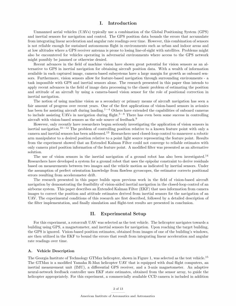
The Georgia Institute of Technology GTMax helicopter, shown in Figure 1, was selected as the test vehicle.15

The GTMax is a modified Yamaha R-Max helicopter UAV that is equipped with dual flight computers, aninertial measurement unit (IMU), a differential GPS receiver, and a 3-axis magnetometer. An adaptiveneural-network feedback controller uses EKF state estimates, obtained from the sensor array, to guide thehelicopter appropriately. For this experiment, a commercially available CCD camera is included in addition

2 of 13


Figure 1. The GTMax UAV helicopter.

to the normal flight hardware configuration, along with an image processor for interpreting visual imagesfrom the camera. The image processor is capable of detecting a dark square against a light background andprovides the square root of the object’s area and the position of the object’s center in the camera image.9

B. Assumptions

It is assumed that the target is a stationary dark 2D square against a light background to simplify therequirements of computationally expensive image processing. The target’s position, orientation, and areaare also known beforehand. Regarding camera geometry, the assumptions are made that the distance fromthe camera to the vehicle center of mass is negligible and that the horizontal and vertical focal lengths arethe same.

III. Position Estimation from Camera Images

The EKF estimates vehicle position using three measurements of a target obtained from camera images:the square root of the target’s area (α) and the pixel y and z positions of the target center in the cameraimage (u and v respectively). Since the position and orientation of the target are known, the vision-basedestimator needs only to determine the pose of the target to resolve the helicopter’s position. This section firstprovides some fundamentals on relating 3D position to 2D images, and then describes the implementationof the EKF.

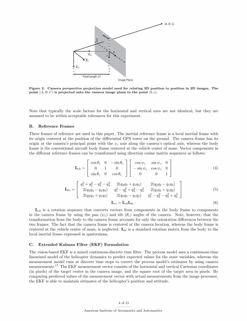
A. Relating 3D Position to 2D Images

A perspective projection model of a pinhole camera allows position in a 2D camera image to be inferredfrom 3D position as shown in Figure 2.9,16 The model projects an arbitrary point (A,B, C) to a pixel point(b, c) on the image plane (the camera image) according to the following relations:

b = fB

A(1)

c = fC

A, (2)

where f is the focal length of the camera. The focal length depends solely on the image width in pixels ofthe camera image (w) and the angle of the field of view (FOV ), both of which are characteristics of thecamera, according to

f =w

2 tan(

FOV2

) . (3)

3 of 13


x

y

z

c

c

c

Image Plane

b

c

(A, B, C)

Focal Length (f)

Figure 2. Camera perspective projection model used for relating 3D position to position in 2D images. Thepoint (A, B, C) is projected onto the camera image plane to the point (b, c).

Note that typically the scale factors for the horizontal and vertical axes are not identical, but they areassumed to be within acceptable tolerances for this experiment.

B. Reference Frames

Three frames of reference are used in this paper. The inertial reference frame is a local inertial frame withits origin centered at the position of the differential GPS tower on the ground. The camera frame has itsorigin at the camera’s principal point with the xc axis along the camera’s optical axis, whereas the bodyframe is the conventional aircraft body frame centered at the vehicle center of mass. Vector components inthe different reference frames can be transformed using direction cosine matrix sequences as follows:

Lcb =

cos θc 0 − sin θc

0 1 0sin θc 0 cos θc

cosψc sin ψc 0− sin ψc cosψc 0

0 0 1

(4)

Lbi =

q21 + q2

2 − q23 − q2

4 2(q2q3 + q1q4) 2(q2q4 − q1q3)2(q2q3 − q1q4) q2

1 − q22 + q2

3 − q24 2(q3q4 + q1q2)

2(q2q4 + q1q3) 2(q3q4 − q1q2) q21 − q2

2 − q23 + q2

4

(5)

Lci = LcbLbi . (6)

Lcb is a rotation sequence that converts vectors from components in the body frame to componentsin the camera frame by using the pan (ψc) and tilt (θc) angles of the camera. Note, however, that thetransformation from the body to the camera frame accounts for only the orientation differences between thetwo frames. The fact that the camera frame is centered at the camera location, whereas the body frame iscentered at the vehicle center of mass, is neglected. Lbi is a standard rotation matrix from the body to thelocal inertial frame expressed in quaternions.

C. Extended Kalman Filter (EKF) Formulation

The vision-based EKF is a mixed continuous-discrete time filter. The process model uses a continuous-timelinearized model of the helicopter dynamics to predict expected values for the state variables, whereas themeasurement model runs at discrete time steps to correct the process model’s estimates by using camerameasurements.17 The EKF measurement vector consists of the horizontal and vertical Cartesian coordinates(in pixels) of the target center in the camera image, and the square root of the target area in pixels. Bycomparing predicted values of the measurement vector with actual measurements from the image processor,the EKF is able to maintain estimates of the helicopter’s position and attitude.

4 of 13


1. Process Model

The process model for the EKF is a dynamic helicopter model that utilizes 16 states: attitude quaternions,position and velocity as components in the inertial reference frame, and accelerometer and gyroscope biases.In the process model phase of the EKF estimation algorithm, two main events occur. First, the stateestimate x is updated using the derivative of the state vector obtained directly from inertial measurements.Simultaneously, the covariance matrix P is updated according to the Differential Lyapunov Equation. Theprocess model can be expressed as the following set of differential equations

˙x(t) = f(x(t), t) (7)P(t) = AP + PAT + Q (8)

where x is the state estimate, f(x(t), t) is the nonlinear helicopter model, P is the error covariance matrix,A is a matrix representing the linearized helicopter dynamics, and Q is a diagonal matrix representing theprocess noise inherent in the system model. Values for the Q matrix were initially set by using rough ap-proximations derived from modeling assumptions, and then tuning the values based on data from subsequentflight tests.

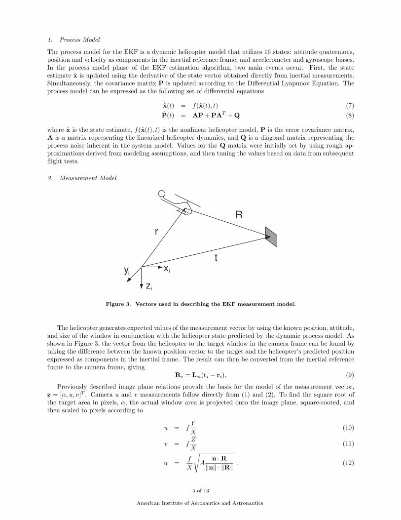
2. Measurement Model

r

t

R

x

z

y i

i

i

Figure 3. Vectors used in describing the EKF measurement model.

The helicopter generates expected values of the measurement vector by using the known position, attitude,and size of the window in conjunction with the helicopter state predicted by the dynamic process model. Asshown in Figure 3, the vector from the helicopter to the target window in the camera frame can be found bytaking the difference between the known position vector to the target and the helicopter’s predicted positionexpressed as components in the inertial frame. The result can then be converted from the inertial referenceframe to the camera frame, giving

Rc = Lci(ti − ri). (9)

Previously described image plane relations provide the basis for the model of the measurement vector,z = [α, u, v]T . Camera u and v measurements follow directly from (1) and (2). To find the square root ofthe target area in pixels, α, the actual window area is projected onto the image plane, square-rooted, andthen scaled to pixels according to

u = fY

X(10)

v = fZ

X(11)

α =f

X

√A

n ·R‖n‖ · ‖R‖ . (12)

5 of 13


Rc = [X,Y, Z]T is the relative position vector of the target window from the helicopter expressed as com-ponents of the camera frame. The vector n is the normal vector of the target window derived from thewindow’s known attitude. The given area of the window is represented by A and f is the camera focal lengthas described before.

The EKF makes use of the measurement model to update the result from the integration of the processmodel given in (7) and (8), at a rate of 10 Hz for both the camera and magnetometer readings. In thisupdate phase of the state estimation, the Kalman gain is first computed. This gain is used as a weighting tofuse the actual camera measurements with the predicted measurements, given by the measurement model in(10) - (12), thus correcting the a priori process model estimate according to the following equations

K = P−CT (CP−CT + V)−1 (13)x = x− + K[z− h(x−)] (14)P = (I−KC)P− (15)

where K is the Kalman gain, V is a diagonal matrix representing measurement noise in the camera sensor, Cis the Jacobian of the measurement vector with respect to the state vector, also denoted by ( ∂z

∂x ), and h(x−)is the predicted measurement vector as given by the measurement model in (10) - (12). Minus superscriptsin the above equations denote a priori values obtained from the process model equations. The results from(13) - (15) are used by the process model in the next time step to further propagate the state vector andthe covariance matrix, and the procedure is repeated. Constant values for the measurement error covariancematrix V were roughly estimated based on the physical properties of the camera such as the focal lengthand dimensions of the CCD array. These parameters could be tuned using data from subsequent flighttests, but the inaccuracies from using an initial approximation were deemed acceptable for the purpose ofdemonstrating the filter’s feasibility.

As can be seen from (13) - (15), the EKF requires the Jacobian matrix of the measurement vectorwith respect to the vehicle states of the helicopter, C, to fuse the camera information with inertial data.Measurements from the camera are only affected by vehicle position and attitude, hence the partial derivativeswith respect to the other state variables (vehicle velocity and accelerometer and gyroscope biases) areidentically zero. The linearization of the measurement model with respect to vehicle position in the localinertial reference frame is obtained from (9) - (12) as

∂z∂ri

=(

∂z∂Rc

)(∂Rc

∂ri

)(16)

∂z∂Rc

=f

X2

√A 0 0

−Y X 0−Z 0 X

(17)

∂Rc

∂ri= −Lci . (18)

The linearized model of the measurement vector with respect to body attitude quaternions is computedin a similar fashion, giving

∂z∂q

=(

∂z∂Rc

)Lcb

(∂Rb

∂q

)(19)

where Rb is the relative position vector of the target’s center from the vehicle, expressed as components ofthe body frame.

It should be noted, however, that there exists a nontrivial latency in the visual information path dueto the computational intensity of the image processing. The time that it takes for the framegrabber toassemble an image, and for the computer to compute the measurement vector, is not negligible and needsto be taken into account. To mitigate this effect, a simple latency compensation scheme is employed. Inthe update phase of the EKF, the onboard computer uses state information that has been stored in memoryfor the latency period of time as opposed to using the most up to date state estimate. This prevents theEKF from comparing the current state estimate information with a camera snapshot that was actuallytaken some time ago. The system latency was estimated empirically from flight test data by finding thelatency value that minimized the least squares error between the predicted camera measurements, foundby applying the measurement model to recorded state data obtained using GPS, and the actual recordedcamera measurements from the flight.

6 of 13


IV. Simulation Results

Simulation tests were used initially to verify the vision-based filter’s performance. In the particularscenario presented in this section, the helicopter begins at a position 120 ft away from a 12.6 ft2 windowand uses only an IMU, a magnetometer, and a camera as sensors for navigation. The helicopter hovers andthen performs a 7.5 ft step up in altitude, a 10 ft step parallel to the window, and a 10 ft step towards thewindow. The state estimates obtained from the vision-based EKF are used in the closed-loop control of thevehicle in this test.

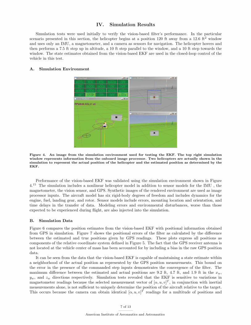
A. Simulation Environment

Figure 4. An image from the simulation environment used for testing the EKF. The top right simulationwindow represents information from the onboard image processor. Two helicopters are actually shown in thesimulation to represent the actual position of the helicopter and the estimated position as determined by theEKF.

Performance of the vision-based EKF was validated using the simulation environment shown in Figure4.15 The simulation includes a nonlinear helicopter model in addition to sensor models for the IMU , themagnetometer, the vision sensor, and GPS. Synthetic images of the rendered environment are used as imageprocessor inputs. The aircraft model has six rigid-body degrees of freedom and includes dynamics for theengine, fuel, landing gear, and rotor. Sensor models include errors, mounting location and orientation, andtime delays in the transfer of data. Modeling errors and environmental disturbances, worse than thoseexpected to be experienced during flight, are also injected into the simulation.

B. Simulation Data

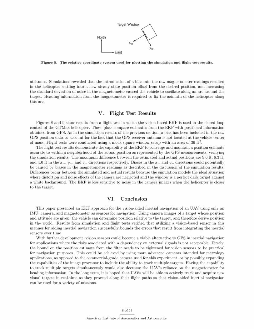
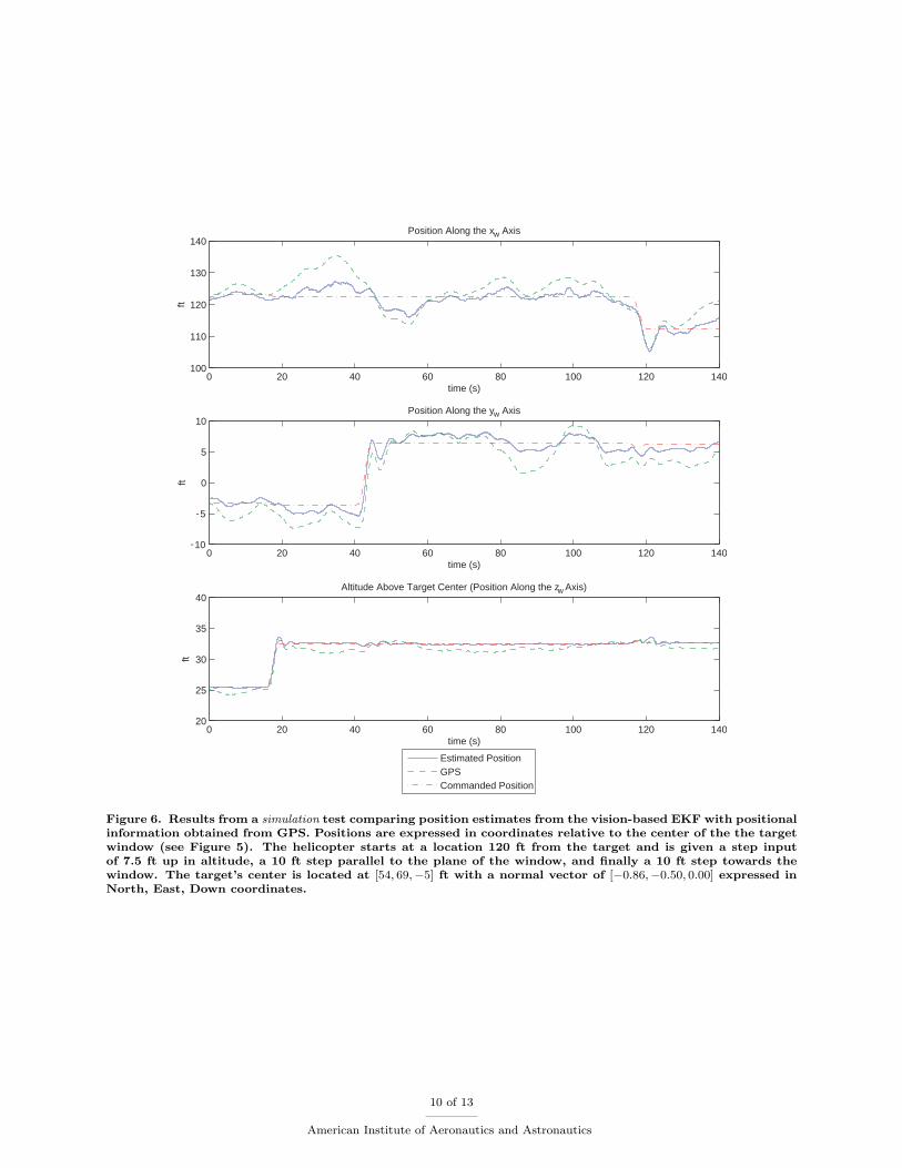
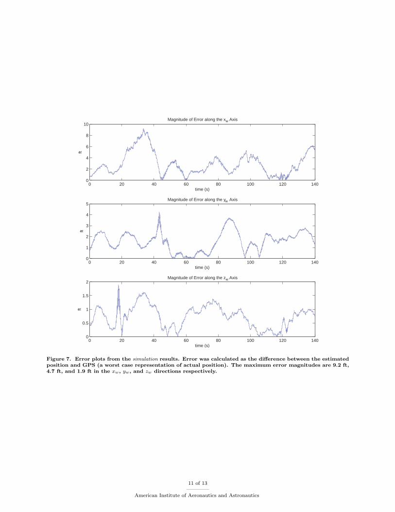
Figure 6 compares the position estimates from the vision-based EKF with positional information obtainedfrom GPS in simulation. Figure 7 shows the positional errors of the filter as calculated by the differencebetween the estimated and true positions given by GPS readings. These plots express all positions ascomponents of the relative coordinate system defined in Figure 5. The fact that the GPS receiver antenna isnot located at the vehicle center of mass has been accounted for by including a bias in the raw GPS positiondata.

It can be seen from the data that the vision-based EKF is capable of maintaining a state estimate withina neighborhood of the actual position as represented by the GPS position measurements. This bound onthe error in the presence of the commanded step inputs demonstrates the convergence of the filter. Themaximum difference between the estimated and actual positions are 9.2 ft, 4.7 ft, and 1.9 ft in the xw,yw, and zw directions respectively. Simulation tests revealed that the EKF is sensitive to variations inmagnetometer readings because the selected measurement vector of [α, u, v]T , in conjunction with inertialmeasurements alone, is not sufficient to uniquely determine the position of the aircraft relative to the target.This occurs because the camera can obtain identical [α, u, v]T readings for a multitude of positions and

7 of 13


North

Eas

y

x

Target Window

w

w

t

Figure 5. The relative coordinate system used for plotting the simulation and flight test results.

attitudes. Simulations revealed that the introduction of a bias into the raw magnetometer readings resultedin the helicopter settling into a new steady-state position offset from the desired position, and increasingthe standard deviation of noise in the magnetometer caused the vehicle to oscillate along an arc around thetarget. Heading information from the magnetometer is required to fix the azimuth of the helicopter alongthis arc.

V. Flight Test Results

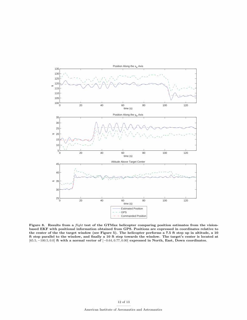
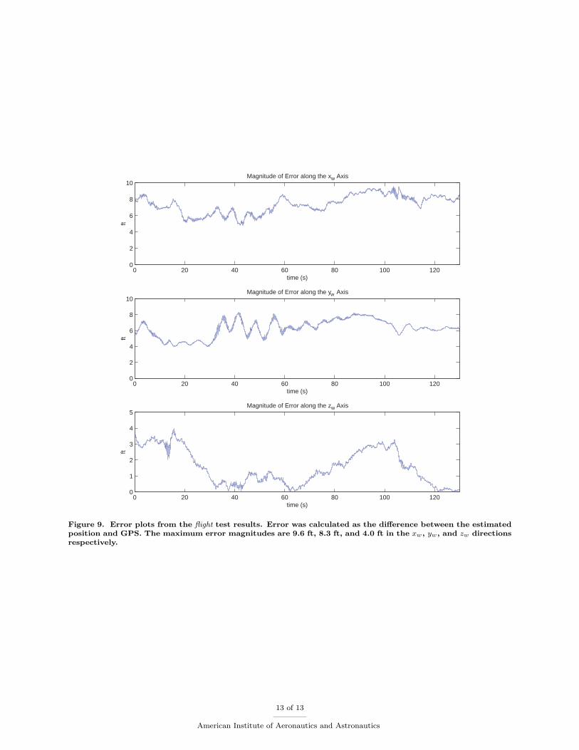
Figures 8 and 9 show results from a flight test in which the vision-based EKF is used in the closed-loopcontrol of the GTMax helicopter. These plots compare estimates from the EKF with positional informationobtained from GPS. As in the simulation results of the previous section, a bias has been included in the rawGPS position data to account for the fact that the GPS receiver antenna is not located at the vehicle centerof mass. Flight tests were conducted using a mock square window setup with an area of 36 ft2.

The flight test results demonstrate the capability of the EKF to converge and maintain a position estimateaccurate to within a neighborhood of the actual position as represented by the GPS measurements, verifyingthe simulation results. The maximum difference between the estimated and actual positions are 9.6 ft, 8.3 ft,and 4.0 ft in the xw, yw, and zw directions respectively. Biases in the xw and yw directions could potentiallybe caused by biases in the magnetometer readings as described in the discussion of the simulation results.Differences occur between the simulated and actual results because the simulation models the ideal situationwhere distortion and noise effects of the camera are neglected and the window is a perfect dark target againsta white background. The EKF is less sensitive to noise in the camera images when the helicopter is closerto the target.

VI. Conclusion

This paper presented an EKF approach for the vision-aided inertial navigation of an UAV using only anIMU, camera, and magnetometer as sensors for navigation. Using camera images of a target whose positionand attitude are given, the vehicle can determine position relative to the target, and therefore derive positionin the world. Results from simulation and flight tests verified that utilizing a vision-based sensor in thismanner for aiding inertial navigation successfully bounds the errors that result from integrating the inertialsensors over time.

With further development, vision sensors could become a viable alternative to GPS in inertial navigationfor applications where the risks associated with a dependency on external signals is not acceptable. Firstly,the bound on the position estimate from the filter needs to be tightened for vision sensors to be practicalfor navigation purposes. This could be achieved by using more advanced cameras intended for metrologyapplications, as opposed to the commercial-grade camera used for this experiment, or by possibly expandingthe capabilities of the image processor to include the ability to track multiple targets. Having the capabilityto track multiple targets simultaneously would also decrease the UAV’s reliance on the magnetometer forheading information. In the long term, it is hoped that UAVs will be able to actively track and acquire newvisual targets in real-time as they proceed along their flight paths so that vision-aided inertial navigationcan be used for a variety of missions.

8 of 13


Acknowledgements

The authors would like to acknowledge contributions of the following people to the work presented in thispaper: Henrik Christophersen, Jincheol Ha, Jeong Hur, Suresh Kannan, Adrian Koller, Alex Moodie, WaynePickell, and Nimrod Rooz. This work is supported by the Active-Vision Control Systems (AVCS) Multi-University Research Initiative (MURI) Program under contract #F49620-03-1-0401 and by the SoftwareEnabled Control (SEC) Program under contracts #33615-98-C-1341 and #33615-99-C-1500.

References

1Saripalli, S., Montogomery, J. F., and Sukhatme, G. S., “Visually Guided Landing of an Unmanned Aerial Vehicle,”Transactions on Robotics and Automation, IEEE, Vol. 19, No. 3, June 2003, pp. 371-380.

2Shakernia, O., Vidal, R., Sharp, C. S., Ma, Y., and Sastry, S., “Multiple View Motion Estimation and Control forLanding an Unmanned Aerial Vehicle,” Proceedings of the International Conference on Robotics and Automation, IEEE, Vol.3, Washington, DC, May 2002, pp. 2793-2798.

3Chatterji, G.B., Menon, P.K., and Sridhar, B., ”GPS/Machine Vision Navigation System for Aircraft,” Transactions onAerospace and Electronic Systems, IEEE, Vol. 33, No. 3, July 1997, pp. 1012-1025.

4Bosse, M., Karl, W. C., Castanon, D., and DeBitetto, P., “A Vision Augmented Navigation System,” Conference onIntelligent Transportation Systems, IEEE, Nov. 1997, pp. 1028-1033.

5Amidi, O., “An Autonomous Vision-Guided Helicopter,” Ph.D. Dissertation, Department of Electrical and ComputerEngineering, Carnegie Mellon University, Pittsburgh, PA, 1996.

6Bernatz, A., and Thielecke, F., “Navigation of a Low Flying VTOL Aircraft With the Help of a Downwards PointingCamera,” Guidance, Navigation, and Control Conference, AIAA, Providence, RI, Aug. 2004.

7Webb, T. P., Prazenica, R. J. Kurdila, A. J., and Lind, R., “Vision-Based State Estimation for Autonomous Micro AirVehicles,” Guidance, Navigation, and Control Conference, AIAA Providence, RI, Aug. 2004.

8Roberts, J., Corke, P., and Buskey, G., ”Low-Cost Flight Control System for a Small Autonomous Helicopter,” Aus-tralasian Conference on Robotics and Automation, Auckland, New Zealand, 2002.

9Proctor, A. A., and Johnson E. N., “Vision-Only Aircraft Flight Control Methods and Test Results,” AIAA Guidance,Navigation, and Control Conference, Providence, RI, Aug. 2004.

10Roberts, B. A., and Vallot, L. C., ”Vision Aided Inertial Navigation,” Record of the Position Location and NavigationSymposium, IEEE, March 1990, pp. 347-352.

11Rehbinder, H., and Ghosh, B. K., ”Multi-Rate Fusion of Visual and Inertial Data,” International Conference on Multi-sensor Fusion and Integration for Intelligent Systems, IEEE, Aug. 2001, pp. 97-102.

12Kaminer, I., Pascoal, A., Kang, W., ”Integrated Vision/Inertial Navigation System Design Using Nonlinear Filtering,”Proceedings of the American Control Conference, Vol. 3, San Diego, CA, 1999, pp. 1910-1914.

13Huster, A., ”Relative Position Sensing by Fusing Monocular Vision and Inertial Rate Sensors,” Ph.D. Dissertation,Department of Electrical Engineering, Stanford University, Stanford, CA, 2004.

14Diel, D., DeBitetto, P., and Teller, S., ”Epipolar Constraints for Vision-Aided Inertial Navigation”, Workshop on Motionand Video Computing, IEEE, Breckenridge, CO, 2005.

15Johnson, E. N., and Schrage, D. P., “System Integration and Operation of a Research Unmanned Aerial Vehicle,” Journalof Aerospace Computing, Information, and Communication, Vol. 1, No. 1, 2004, pp. 5-18.

16Russell, S. J., and Norvig, P., Artificial Intelligence: A Modern Approach, Prentice Hall, New Jersey, 1995, pp. 725-742.17Gelb, A. (ed.), Applied Optimal Estimation, The MIT Press, Cambridge, MA, 1974, pp. 102-110, 182-190.

9 of 13


0 20 40 60 80 100 120 14010

5

0

5

10Position Along the yw Axis

time (s)

ft

0 20 40 60 80 100 120 140100

110

120

130

140Position Along the xw Axis

time (s)

ft

0 20 40 60 80 100 120 14020

25

30

35

40Altitude Above Target Center (Position Along the zw Axis)

time (s)

ft

Estimated PositionGPSCommanded Position

-

-

Figure 6. Results from a simulation test comparing position estimates from the vision-based EKF with positionalinformation obtained from GPS. Positions are expressed in coordinates relative to the center of the the targetwindow (see Figure 5). The helicopter starts at a location 120 ft from the target and is given a step inputof 7.5 ft up in altitude, a 10 ft step parallel to the plane of the window, and finally a 10 ft step towards thewindow. The target’s center is located at [54, 69,−5] ft with a normal vector of [−0.86,−0.50, 0.00] expressed inNorth, East, Down coordinates.

10 of 13


0 20 40 60 80 100 120 1400

1

2

3

4

5Magnitude of Error along the yw Axis

ft

time (s)

0 20 40 60 80 100 120 1400

2

4

6

8

10Magnitude of Error along the xw Axis

ft

time (s)

0 20 40 60 80 100 120 1400

0.5

1

1.5

2Magnitude of Error along the zw Axis

ft

time (s)

Figure 7. Error plots from the simulation results. Error was calculated as the difference between the estimatedposition and GPS (a worst case representation of actual position). The maximum error magnitudes are 9.2 ft,4.7 ft, and 1.9 ft in the xw, yw, and zw directions respectively.

11 of 13


0 20 40 60 80 100 1205

10

15

20

25

30

35Position Along the yw Axis

time (s)

ft

0 20 40 60 80 100 120100

105

110

115

120

125

130

135Position Along the xw Axis

time (s)

ft

0 20 40 60 80 100 12025

30

35

40

45Altitude Above Target Center

time (s)

ft

Estimated PositionGPSCommanded Position

Figure 8. Results from a flight test of the GTMax helicopter comparing position estimates from the vision-based EKF with positional information obtained from GPS. Positions are expressed in coordinates relative tothe center of the the target window (see Figure 5). The helicopter performs a 7.5 ft step up in altitude, a 10ft step parallel to the window, and finally a 10 ft step towards the window. The target’s center is located at[65.5,−100.5, 0.0] ft with a normal vector of [−0.64, 0.77, 0.00] expressed in North, East, Down coordinates.

12 of 13


0 20 40 60 80 100 1200

2

4

6

8

10Magnitude of Error along the yw Axis

ft

time (s)

0 20 40 60 80 100 1200

2

4

6

8

10Magnitude of Error along the xw Axis

ft

time (s)

0 20 40 60 80 100 1200

1

2

3

4

5Magnitude of Error along the zw Axis

ft

time (s)

Figure 9. Error plots from the flight test results. Error was calculated as the difference between the estimatedposition and GPS. The maximum error magnitudes are 9.6 ft, 8.3 ft, and 4.0 ft in the xw, yw, and zw directionsrespectively.

13 of 13


vision-aided inertial navigation for flight control · the gtmax is a modiﬁed yamaha r-max...

Documents