University of Central Florida University of Central Florida

STARS STARS

Electronic Theses and Dissertations, 2004-2019

2018

Visionary Ophthalmics: Confluence of Computer Vision and Deep Visionary Ophthalmics: Confluence of Computer Vision and Deep

Learning for Ophthalmology Learning for Ophthalmology

Dustin Morley University of Central Florida

Part of the Computer Sciences Commons

Find similar works at: https://stars.library.ucf.edu/etd

University of Central Florida Libraries http://library.ucf.edu

This Doctoral Dissertation (Open Access) is brought to you for free and open access by STARS. It has been accepted

for inclusion in Electronic Theses and Dissertations, 2004-2019 by an authorized administrator of STARS. For more

information, please contact STARS@ucf.edu.

STARS Citation STARS Citation Morley, Dustin, "Visionary Ophthalmics: Confluence of Computer Vision and Deep Learning for Ophthalmology" (2018). Electronic Theses and Dissertations, 2004-2019. 5793. https://stars.library.ucf.edu/etd/5793

VISIONARY OPHTHALMICS: CONFLUENCE OF COMPUTER VISION AND DEEPLEARNING FOR OPHTHALMOLOGY

by

DUSTIN MORLEYM.S. University of Central Florida, 2016B.S. University of Central Florida, 2012

A dissertation submitted in partial fulfilment of the requirementsfor the degree of Doctor of Philosophyin the Department of Computer Science

in the College of Engineering and Computer Scienceat the University of Central Florida

Orlando, Florida

Spring Term2018

Major Professor: Hassan Foroosh

c© 2018 Dustin Morley

ii

ABSTRACT

Ophthalmology is a medical field ripe with opportunities for meaningful application of computer

vision algorithms. The field utilizes data from multiple disparate imaging techniques, ranging

from conventional cameras to tomography, comprising a diverse set of computer vision chal-

lenges. Computer vision has a rich history of techniques that can adequately meet many of these

challenges. However, the field has undergone something of a revolution in recent times as deep

learning techniques have sprung into the forefront following advances in GPU hardware. This de-

velopment raises important questions regarding how to best leverage insights from both modern

deep learning approaches and more classical computer vision approaches for a given problem. In

this dissertation, we tackle challenging computer vision problems in ophthalmology using methods

all across this spectrum. Perhaps our most significant work is a highly successful iris registration

algorithm for use in laser eye surgery. This algorithm relies on matching features extracted from the

structure tensor and a Gabor wavelet – a classically driven approach that does not utilize modern

machine learning. However, drawing on insight from the deep learning revolution, we demonstrate

successful application of backpropagation to optimize the registration significantly faster than the

alternative of relying on finite differences. Towards the other end of the spectrum, we also present

a novel framework for improving RANSAC segmentation algorithms by utilizing a convolutional

neural network (CNN) trained on a RANSAC-based loss function. Finally, we apply state-of-the-

art deep learning methods to solve the problem of pathological fluid detection in optical coherence

tomography images of the human retina, using a novel retina-specific data augmentation technique

to greatly expand the data set. Altogether, our work demonstrates benefits of applying a holistic

view of computer vision, which leverages deep learning and associated insights without neglecting

techniques and insights from the previous era.

iii

This dissertation is dedicated to my loving and supportive wife, Rebecca. Her patience and

encouragement were critical throughout my graduate studies. I am also grateful to the many

family members, friends, and colleagues who have regularly and enthusiastically offered

encouragement.

iv

ACKNOWLEDGMENTS

This work would not have been possible without the financial support of LENSAR, Inc. In addition

to the financial support, LENSAR provided an ideal environment for me to complete my studies

while working full time, and I am extremely grateful to LENSAR for that. To this end, I would

like to specifically thank Gary Gray and Alan Connaughton for the roles they played in establishing

and maintaining this environment. I would also like to thank Glen Martin, Art Newton, and Valas

Teuma for their overall support and all of the great technical conversations we have had, as well as

Keith Peck for providing valuable feedback during the development of some of the novel statistical

methods used in this dissertation.

I am grateful to many UCF professors for their instruction and guidance, as I can honestly say that

I thoroughly enjoyed every course I took throughout my time as a graduate student in computer

science. I would especially like to thank Dr. Hassan Foroosh, the chairman of my dissertation

committee, for his professional and academic guidance. Also from my committee, I would like to

thank Dr. Ulas Bagci for connecting me to the field of OCT image analysis, and Dr. Boqing Gong

for planting the seeds that led to my research and contributions at the boundary between machine

learning and more traditional computer vision methods.

v

TABLE OF CONTENTS

LIST OF FIGURES . . . . . . . . . . . . . . . . . . . . . . . . . . . . . . . . . . . . . . xi

LIST OF TABLES . . . . . . . . . . . . . . . . . . . . . . . . . . . . . . . . . . . . . . . xiv

CHAPTER 1: INTRODUCTION . . . . . . . . . . . . . . . . . . . . . . . . . . . . . . . 1

Medical Computer Vision . . . . . . . . . . . . . . . . . . . . . . . . . . . . . . . . . . 3

Computer Vision in Ophthalmology . . . . . . . . . . . . . . . . . . . . . . . . . . . . 4

Designed Algorithms vs. Learned Algorithms . . . . . . . . . . . . . . . . . . . . . . . 5

Backpropagation - With or Without Machine Learning . . . . . . . . . . . . . . . . . . 7

CHAPTER 2: LITERATURE REVIEW . . . . . . . . . . . . . . . . . . . . . . . . . . . 11

RANSAC . . . . . . . . . . . . . . . . . . . . . . . . . . . . . . . . . . . . . . . . . . 11

Automatic Iris Registration . . . . . . . . . . . . . . . . . . . . . . . . . . . . . . . . . 12

Convolutional Neural Networks . . . . . . . . . . . . . . . . . . . . . . . . . . . . . . 16

Backpropagation . . . . . . . . . . . . . . . . . . . . . . . . . . . . . . . . . . . . . . 19

Retina Fluid . . . . . . . . . . . . . . . . . . . . . . . . . . . . . . . . . . . . . . . . . 20

CHAPTER 3: COMPUTING CYCLOTORSION IN REFRACTIVE CATARACT SURGERY

vi

21

Relevant Prior Work . . . . . . . . . . . . . . . . . . . . . . . . . . . . . . . . . . . . . 23

Proposed Method . . . . . . . . . . . . . . . . . . . . . . . . . . . . . . . . . . . . . . 26

Boundary Detection . . . . . . . . . . . . . . . . . . . . . . . . . . . . . . . . . . 27

Filtering and Unwrapping the Iris . . . . . . . . . . . . . . . . . . . . . . . . . . . 33

Feature Extraction . . . . . . . . . . . . . . . . . . . . . . . . . . . . . . . . . . . 35

Measuring Correlation Strength . . . . . . . . . . . . . . . . . . . . . . . . . . . 37

Extracting and Applying the Angle of Cyclotorsion . . . . . . . . . . . . . . . . . 40

Data Collection and Validation . . . . . . . . . . . . . . . . . . . . . . . . . . . . . . . 42

Experiments . . . . . . . . . . . . . . . . . . . . . . . . . . . . . . . . . . . . . . . . . 48

Impact of Pupil Dilation . . . . . . . . . . . . . . . . . . . . . . . . . . . . . . . 48

Efficacy of Masking Out Eyelids . . . . . . . . . . . . . . . . . . . . . . . . . . . 49

Importance of Centration for Unwrapping . . . . . . . . . . . . . . . . . . . . . . 49

Radial Shear Efficacy and Error Rates . . . . . . . . . . . . . . . . . . . . . . . . 50

Discussion . . . . . . . . . . . . . . . . . . . . . . . . . . . . . . . . . . . . . . . . . . 60

Conclusion . . . . . . . . . . . . . . . . . . . . . . . . . . . . . . . . . . . . . . . . . 62

CHAPTER 4: IRIS REGISTRATION WITH OPTIMIZED UNWRAPPING . . . . . . . . 63

vii

Introduction . . . . . . . . . . . . . . . . . . . . . . . . . . . . . . . . . . . . . . . . . 63

Method . . . . . . . . . . . . . . . . . . . . . . . . . . . . . . . . . . . . . . . . . . . 64

Review of Prior Method . . . . . . . . . . . . . . . . . . . . . . . . . . . . . . . . 66

Optimizing the Unwrapping Center . . . . . . . . . . . . . . . . . . . . . . . . . . 69

Experiments . . . . . . . . . . . . . . . . . . . . . . . . . . . . . . . . . . . . . . . . . 77

Registration Efficacy . . . . . . . . . . . . . . . . . . . . . . . . . . . . . . . . . 77

Benefits of Backpropagation . . . . . . . . . . . . . . . . . . . . . . . . . . . . . 81

Significance of Final Unwrapping Center . . . . . . . . . . . . . . . . . . . . . . 83

Conclusion . . . . . . . . . . . . . . . . . . . . . . . . . . . . . . . . . . . . . . . . . 86

CHAPTER 5: IMPROVING RANSAC SEGMENTATION THROUGH CNN ENCAPSU-

LATION . . . . . . . . . . . . . . . . . . . . . . . . . . . . . . . . . . . . 88

Introduction . . . . . . . . . . . . . . . . . . . . . . . . . . . . . . . . . . . . . . . . . 88

Related Work . . . . . . . . . . . . . . . . . . . . . . . . . . . . . . . . . . . . . . . . 91

Method . . . . . . . . . . . . . . . . . . . . . . . . . . . . . . . . . . . . . . . . . . . 93

Preprocessing . . . . . . . . . . . . . . . . . . . . . . . . . . . . . . . . . . . . . 93

Feature Extraction . . . . . . . . . . . . . . . . . . . . . . . . . . . . . . . . . . . 94

Clutter Removal . . . . . . . . . . . . . . . . . . . . . . . . . . . . . . . . . . . . 95

viii

RANSAC Fitting and Backpropagation . . . . . . . . . . . . . . . . . . . . . . . 96

Parameters . . . . . . . . . . . . . . . . . . . . . . . . . . . . . . . . . . . . . . . 98

Experiments . . . . . . . . . . . . . . . . . . . . . . . . . . . . . . . . . . . . . . . . . 99

Base Configuration Definition . . . . . . . . . . . . . . . . . . . . . . . . . . . . 100

Base Configuration Results . . . . . . . . . . . . . . . . . . . . . . . . . . . . . . 100

Hyperparameter Variation . . . . . . . . . . . . . . . . . . . . . . . . . . . . . . . 105

Alternate Configurations . . . . . . . . . . . . . . . . . . . . . . . . . . . . . . . 106

Reduced Training Set . . . . . . . . . . . . . . . . . . . . . . . . . . . . . . . . . 107

Discussion . . . . . . . . . . . . . . . . . . . . . . . . . . . . . . . . . . . . . . . . . . 107

CHAPTER 6: SIMULTANEOUS DETECTION AND QUANTIFICATION OF RETINAL

FLUID WITH DEEP LEARNING . . . . . . . . . . . . . . . . . . . . . . . 109

Introduction . . . . . . . . . . . . . . . . . . . . . . . . . . . . . . . . . . . . . . . . . 109

Related Work . . . . . . . . . . . . . . . . . . . . . . . . . . . . . . . . . . . . . . . . 109

Method . . . . . . . . . . . . . . . . . . . . . . . . . . . . . . . . . . . . . . . . . . . 110

Pre-Processing. . . . . . . . . . . . . . . . . . . . . . . . . . . . . . . . . . . . . 110

Data Augmentation. . . . . . . . . . . . . . . . . . . . . . . . . . . . . . . . . . . 111

CNN Architecture. . . . . . . . . . . . . . . . . . . . . . . . . . . . . . . . . . . 112

ix

Post-Processing. . . . . . . . . . . . . . . . . . . . . . . . . . . . . . . . . . . . . 116

Results . . . . . . . . . . . . . . . . . . . . . . . . . . . . . . . . . . . . . . . . . . . . 117

Experiments on RETOUCH Data Set . . . . . . . . . . . . . . . . . . . . . . . . . 118

Experiments on Alternate Data Set . . . . . . . . . . . . . . . . . . . . . . . . . . 121

Conclusion . . . . . . . . . . . . . . . . . . . . . . . . . . . . . . . . . . . . . . . . . 124

CHAPTER 7: CONCLUSION . . . . . . . . . . . . . . . . . . . . . . . . . . . . . . . . 125

APPENDIX : COPYRIGHT INFORMATION . . . . . . . . . . . . . . . . . . . . . . . 129

LIST OF REFERENCES . . . . . . . . . . . . . . . . . . . . . . . . . . . . . . . . . . . 135

x

LIST OF FIGURES

Figure 2.1: Google Scholar search results for "Convolutional Neural Network" over time. 17

Figure 3.1: Boundary detection for a LLS image . . . . . . . . . . . . . . . . . . . . . 29

Figure 3.2: Boundary detection for a Cassini image . . . . . . . . . . . . . . . . . . . 30

Figure 3.3: Image filtering procedure for eyelid interference detection. . . . . . . . . . 32

Figure 3.4: Example results of eyelid interference detection. . . . . . . . . . . . . . . 32

Figure 3.5: Locating the innermost suction ring in an LLS image. . . . . . . . . . . . 33

Figure 3.6: Unwrapped, DOG filtered iris (LLS top, topographer bottom). . . . . . . . 35

Figure 3.7: Correlation measures as a function of proposed cyclotorsion angle. . . . . 39

Figure 3.8: Confidence score function based on peak height ratio. . . . . . . . . . . . 41

Figure 3.9: Example registration result with highlighted matching sections. . . . . . . 43

Figure 3.10: Correlation plots extended to ±180 degrees. . . . . . . . . . . . . . . . . . 46

Figure 3.11: Cyclotorsion-corrected correlation coefficient as a function of pupil size

difference. . . . . . . . . . . . . . . . . . . . . . . . . . . . . . . . . . . 48

Figure 3.12: Correlation and max noise level measures are approximately normal. . . . 53

Figure 4.1: Visualization of the iris registration algorithm in Chapter 3. . . . . . . . . 65

xi

Figure 4.2: Flowchart of the optimization loop within the iris registration algorithm. . . 66

Figure 4.3: Graphic demonstrating the effect of changing the unwrapping center on the

angular location of features. . . . . . . . . . . . . . . . . . . . . . . . . . 69

Figure 4.4: Surface plot of the registration correlation measure as a function of the LLS

image unwrapping center (relative to the pupil center). . . . . . . . . . . . 70

Figure 4.5: Example outputs of our static pupil dilation model. . . . . . . . . . . . . . 84

Figure 4.6: Example outputs of our dynamic pupil dilation model. . . . . . . . . . . . 85

Figure 4.7: Comparison between the static (left) and dynamic (right) dilation models. . 86

Figure 5.1: Our method for improving RANSAC segmentation performance by CNN

encapsulation. . . . . . . . . . . . . . . . . . . . . . . . . . . . . . . . . 90

Figure 5.2: Pupil segmentation error distributions before (top) and after (bottom) train-

ing, using our base configuration. . . . . . . . . . . . . . . . . . . . . . . . 101

Figure 5.3: Pupil edge precision, recall, and F1 score distributions before (top) and

after (bottom) training, using our base configuration. . . . . . . . . . . . . 102

Figure 5.4: Learned alterations to the convolutional filters in the network, shown in the

spirit of [2]. . . . . . . . . . . . . . . . . . . . . . . . . . . . . . . . . . . 104

Figure 5.5: Illustration of challenging images in the data set. . . . . . . . . . . . . . . 105

Figure 6.1: Examples of myopic warping. . . . . . . . . . . . . . . . . . . . . . . . . 112

xii

Figure 6.2: Fundamental processing units on the encoder (left, blue) and decoder (right,

orange) portions of our CNN. . . . . . . . . . . . . . . . . . . . . . . . . 113

Figure 6.3: Endgame for the CNN. . . . . . . . . . . . . . . . . . . . . . . . . . . . . 114

Figure 6.4: Examples on which our method performed extremely well. . . . . . . . . . 118

Figure 6.5: (a) Examples on which our method struggled, and (b) examples on which

our IRF results are arguably more accurate than the reference standard. . . 119

Figure 6.6: Fluid detection ROC curves obtained by our method in the RETOUCH

challenge. . . . . . . . . . . . . . . . . . . . . . . . . . . . . . . . . . . . 121

xiii

LIST OF TABLES

Table 3.1: Summary of manual validation results. . . . . . . . . . . . . . . . . . . . 44

Table 3.2: Signal and background statistics for varying amounts of max radial shear. . 51

Table 3.3: Basic probability statistics for varying amounts of max radial shear. . . . . 56

Table 3.4: Probability statistics for different acceptance thresholds (T). . . . . . . . . 59

Table 4.1: Correlation increases as a result of optimizing the unwrapping center. . . . 78

Table 4.2: Conservative estimates of registration success rates, with a fixed false reg-

istration rate of 3× 10−5. . . . . . . . . . . . . . . . . . . . . . . . . . . 80

Table 4.3: Computation time benefits of backpropagation in iris registration. . . . . . 82

Table 4.4: Differences in final outputs between finite difference and backpropagation. 83

Table 5.1: Accuracy results for our base configuration. . . . . . . . . . . . . . . . . . 102

Table 5.2: Edge map evaluation for our base configuration. . . . . . . . . . . . . . . 102

Table 6.1: Complete architecture specification for our deep ResNet encoder-decoder

CNN. . . . . . . . . . . . . . . . . . . . . . . . . . . . . . . . . . . . . . 115

Table 6.2: Quantitative results on RETOUCH data set. . . . . . . . . . . . . . . . . . 120

Table 6.3: Quantitative results on alternate data set. . . . . . . . . . . . . . . . . . . . 123

xiv

CHAPTER 1: INTRODUCTION

The medical field of ophthalmology has become an active area for the application of computer

vision algorithms, especially in recent years. The field utilizes a variety of imaging systems for

different purposes, which naturally results in a diverse space of computer vision algorithms be-

ing utilized to analyze image data from these systems. For example, femtosecond laser cataract

surgery relies on computer vision algorithms for treatment planning and execution. Some of these

algorithms operate on "straight-on" images of the eye acquired with a conventional camera, while

others operate on cross-sectional images of the eye acquired with either a Scheimpflug camera

or optical coherence tomography (OCT). As another example, computer vision algorithms often

assist in analysis of retina health, operating on images acquired by OCT. Thus, in multiple ways,

ophthalmology is a field in which computer vision is regularly applied toward the end of improving

human vision.

This dissertation presents multiple significant contributions to this area, which have been previ-

ously published in outlets including IEEE Transactions on Biomedical Engineering (TBME) and

Proceedings of the IEEE Conference on Computer Vision and Pattern Recognition (CVPR). These

published works do not all directly build on each other, and in that sense they have a degree of

independence between them. We aim to present these works within the unified framework of oph-

thalmic computer vision. Along the way, important questions in computer vision are considered,

such as the fundamental distinguishing features of biomedical computer vision and the extent of

machine learning’s applicability in computer vision. We hope that these discussions will encour-

age readers to consider alternate perspectives, and ultimately play a role in the generation of new

and exciting ideas.

The first contribution presented is an algorithm for registering two images of the eye using the

1

iris patterns. More specifically, the algorithm is applied in the context of laser eye surgery, where

rotational misalignment of astigmatism treatments is a clinically significant issue due to the phe-

nomenon of cyclotorsion. An interesting thing about the problem of iris registration is that there

is a huge amount of relevant published work that is not at all connected to medicine. We are re-

ferring here to work on iris recognition, or using the iris pattern to identify a person for security

purposes. The very same factors that render it possible to identify a person based on his or her

iris pattern also make the iris a good tracking target for image registration. Thus, we leveraged in-

sights from iris recognition literature alongside the relatively limited prior work on iris registration

in the design of our algorithm, which is published in TBME. Since that publication, the algorithm

has been developed even further to incorporate additional degrees of freedom into the registration,

resulting in increased efficacy as well as the possibility of obtaining additional useful information

from the new components of the registration. Interestingly, the methodology for doing so involves

backpropagation, a technique normally only used in neural networks.

The next contribution is an analysis of the potential for deep learning techniques to be leveraged

for improving RANSAC-based segmentation algorithms. Obviously, RANSAC-based segmenta-

tion is not specific to ophthalmology by any stretch. However, it is extremely well suited to several

segmentation problems in ophthalmology due to the fact that many anatomical surfaces of the eye

fit very well to simple shapes such as circles, ellipses, and parabolas. Indeed, we demonstrated our

approach on the problem of pupil segmentation. We showed that it was possible to take an exist-

ing high performance RANSAC algorithm, convert it "as is" into a convolutional neural network

(CNN), and finetune that CNN on a novel RANSAC loss function to make it perform even better.

This work was presented at CVPR 2017.

The final contribution is a direct application of deep learning to detection and segmentation of

pathological retina fluid in OCT images. A deep CNN was constructed to perform simultaneous

detection and segmentation by outputting voxelwise probabilities for each of three fluid types. The

2

CNN embodied both ResNet and Encoder-Decoder design concepts, meaning that "skip layers"

were utilized and feature map sizes transition from full size to smaller sizes and then back to full

size for the final output. The CNN was trained on images from three different OCT devices. Our

method won second place for the detection task in the RETOUCH Grand Challenge at MICCAI

2017.

Medical Computer Vision

There are many factors that serve to make medical computer vision distinct from other areas of

computer vision. Perhaps the most basic difference is that the images being analyzed are often (al-

though not always) acquired by something other than a conventional camera. Even in cases where

a conventional camera is used in medicine, the resulting images can still differ greatly from "natu-

ral" images in terms of scale. A high resolution image of a specific body part captures abundantly

more detail than a natural image of the entire person (or even just the person’s face), but absolutely

no information about the environment the person is in when the image was acquired. In other

words, the scope of visible objects in the image is completely different. This fact is directly tied

to radical differences in the types of problems attempting to be solved in medical computer vision.

While natural computer vision is often concerned with trying to discern and leverage context in

order to find out what is "basically going on" in an image that could have come from just about

anywhere, medical computer vision asks extremely detailed questions about specific objects while

generally assuming a large amount of context to be known up front (i.e., a system for analyzing

brain images would almost always assume up front that its input images are indeed images of the

brain, and it would potentially make several additional assumptions based on knowledge of the

imaging device). There are also significant differences in how successful algorithms are utilized.

In particular, medical computer vision systems generally require a much larger degree of certainty

3

before making decisions; this can be thought of as a "do no harm" philosophy which is generally

not necessary in other areas of computer vision. What this means practically is that false positives

and false negatives are rarely of equal importance in medical computer vision, and so automated

systems will tend to be biased toward the "safe side." This can of course be the case in non-medical

computer vision at times as well (such as security systems allowing access to a building or device

based on facial recognition), but it is less common.

Computer Vision in Ophthalmology

Ophthalmology is the branch of medicine concerned with the eye. It serves as a particularly in-

teresting application domain of medical computer vision, not only because of the delightful irony

of using computer vision to improve human vision, but also because it has a high dependence

on both conventional cameras and tomography. For example, conventional cameras are used for

cornea topography and eye tracking, while optical coherence tomography (OCT) is used to image

the retina. Interestingly, some parts of the eye are amenable to analysis through multiple imaging

modalities. The anterior segment of the eye (the portion of the eye between the front of the cornea

and the back of the lens) is perhaps the best example of this - both OCT and Scheimpflug cameras

have been successfully used to obtain quality images of the cornea and lens.

One of the more exciting areas of ophthalmic computer vision is laser eye surgery, due to the ex-

ceedingly high level of reliance on automated computer vision algorithms for these procedures. In

femtosecond laser-assisted cataract surgery, the LENSAR system 1 performs automatic segmen-

tation of cornea, lens, pupil, and limbus, as well as automatic registration of the imaged iris to a

preoperative image from an external topographer, and these outputs directly define the final treat-

1The LENSAR laser system is a commercial femtosecond laser platform developed and manufactured byLENSAR, Inc. with 510k approvals for a variety of procedures associated with cataract surgery. For more infor-mation, visit their website at www.lensar.com.

4

ment delivered to the eye. The surgeon’s role is limited to planning the pattern geometry, "docking"

the patient to the system by attaching a suction ring, and of course stopping execution of the treat-

ment if anything seems amiss. The surgeon may also make manual corrections to the cornea and

lens segmentations, but this is quite rare. Competing systems also automate several (but not all)

of these steps, and LASIK procedures have similar levels of automated computer vision as well.

Indeed, it is quite difficult to think of another type of surgery that relies on automated computer

vision software as much as laser eye surgery.

At the opposite end of the spectrum (at least in the present day and age), retina care is far less

dependent on computer vision. However, continued improvements to the quality of OCT images

of the retina are beginning to allow for computer vision to assist here as well. Some examples

are automatic segmentation of retina layers and automatic detection of pathological fluid buildup.

Although there is no obvious scenario in the foreseeable future in which the outputs of computer

vision algorithms accomplishing these tasks can define treatment in a form that can be executed

by a machine (as is the case for laser eye surgery in the anterior segment), these algorithms can

nevertheless save retina specialists a lot of time. Hopefully, this line of development can ultimately

allow a greater number of patients to receive appropriate care.

Designed Algorithms vs. Learned Algorithms

Today, one of the fundamental questions of virtually all algorithm design is how much machine

learning can (or should) be leveraged. This question has become especially prominent in the area

of computer vision, where deep learning methods have become state-of-the-art for a variety of

difficult tasks (the most well-known example being object recognition). Deep learning methods

are often thought to require a "large" data set, which would preclude its use for many medical

applications in which it may not be possible to obtain such a data set. However, this may not

5

actually be the case. The practice of data augmentation (artificially generating additional data

from the original data set) is on the rise, and it can be quite fruitful when expertise in the field

is leveraged in the formulation of the data augmentation approach. A great example of this is

presented in Chapter 6 of this dissertation, where a novel technique called myopic warping is

applied to OCT images of the retina. The idea presented by the ophthalmologist participating

in the work was that it should be possible to take any cross-sectional retina image and make it

look more myopic (meaning the center of the retina is further away from the rest of the eye).

We were able to develop a mathematical formulation that accomplished this, and it proved to be

extremely beneficial to the performance of our deep learning algorithm for retina fluid detection

and segmentation. The reason that this was effective is because the artificially generated images

looked like real retina images but were significantly different from the original images. Equally

important is the fact that no manual labeling was required for the artificially generated images,

due to the fact that the ground truth fluid maps could be warped in exactly the same manner as

the images. Thus, data augmentation at its best provides at least two clear benefits: it improves

performance on the desired task, and it increases the efficiency of data preparation.

On the other hand, there are many problems that can be solved without relying on deep learning.

Although in general it would still be possible to formulate an approach utilizing deep learning to

solve these problems, it may simply not be feasible for a variety of reasons. For example, a high-

end graphics card (or access to one through a cloud computing interface) may not be available in

the system running the algorithm. In Chapter 3, a highly successful algorithm for automatic iris

registration is presented. This algorithm does not utilize any machine learning, and it has been

used in thousands of cataract surgeries performed with the LENSAR laser system. In this scenario,

it is natural to adopt a philosophy of "if it ain’t broke, don’t fix it!" with regard to the possibility of

attempting to replace some of the steps with deep learning algorithms. However, leveraging deep

learning in this type of scenario might be more palatable if the algorithmic framework could remain

6

unchanged, the new algorithm could be initialized to perform identically or near-identically to the

previous algorithm before any training occurs, and the loss function used in training is directly

aligned with the end goal of the complete algorithm. This motivated the work presented in Chapter

5, in which a RANSAC algorithm for pupil segmentation is embedded as-is into a convolutional

neural network and fine-tuned with a novel RANSAC loss function.

Backpropagation - With or Without Machine Learning

Backpropagation serves as the algorithmic backbone to the deep learning approaches that have

revolutionized many areas of computer vision in recent years. Without it, deep neural networks

of any kind would require prohibitively long training times - even on a modern high-end graphics

card. Undoubtedly, the field of deep learning would not even exist as anything beyond an academic

exercise if not for backpropagation.

The operation of backpropagation is conceptually very simple. Consider M functions f1, f2, ...fM

with corresponding parameter sets θ1, θ2, ...θM each defined and differentiable on RN , where the

composition of these functions on some input x produces some merit value T :

fM(fM−1(...f1(x, θ1), θM−1), θM) = T (1.1)

The functions are considered optimized when T is either maximized or minimized, depending on

the problem. Note that the way we have written it, fM corresponds to the merit (or loss) function.

We will assume a maximization goal, without loss of generality (since one can always convert such

a maximization problem to minimization by tacking on a negative scaling function to the end of the

function composition). The maximization is achieved through some variation of gradient ascent,

7

updating the modifiable parameters on each iteration according to the following generic update

rule:

θt+1k = θtk + αt

dT

dθtk+ βt (1.2)

dT

dθtk=dT

dfk

dfkdθtk

=

(dT

dfM

M−1∏i=k

dfi+1

dfi

)dfkdθtk

(1.3)

The iteration-dependent terms α and β allow for techniques such as learning rate decay and mo-

mentum, but the most critical component is the computation of the derivative. Following a forward

pass through the function composition, the derivative of T with respect to the last function fM

can be immediately computed, and this value is propagated back to the previous function fM−1 to

allow computation of that derivative, so on and so forth all the way back to the earliest function

in the sequence containing modifiable parameters. Thus, backpropagation in its truest sense is

simply propagation of derivatives backward through a network of function compositions. From

an implementation perspective we would be remiss if we did not point out that the functions do

not necessarily have to form a single "chain" from first to last; as long as the functions can be

arranged in a directed acyclic graph, backpropagation can be executed. In neural networks, the

most popular examples leveraging this fact are GoogleNet [51] and ResNet [50]. However, from a

theoretical perspective, our description is still sufficiently generic, as there is nothing that prevents

any fk from consisting of a sum, concatenation, etc. of multiple sub-functions. The main point is

that each fk can be any differentiable function, without regard for whether the function could be

expected to appear in a neural network.

Despite the immense success of backpropagation in deep learning, very little work has been done

examining the applicability of backpropagation to algorithms outside the context of machine learn-

8

ing. This is somewhat surprising, because in theory any lengthy optimization routine involving

more than one parameter would stand to gain significant improvements in computation time by

employing backpropagation. However, this appears to be frequently overlooked. A basic Google

search for "backpropagation" returns results that almost universally identify it directly with artifi-

cial neural networks, rather than as a method generic to any application of sequential differentiable

computatons. We argue that backpropagation merits more attention as an algorithm in its own right

rather than purely as a neural network tool.

One might try to argue that we are getting too caught up in semantics. Here is why we disagree

with that assessment. Consider an algorithm accomplishing some task, where said algorithm looks

nothing like a neural network. Next, let this algorithm possess a gradient descent loop optimizing

some number of parameters to this algorithm, where these parameters could not be classified as

"neurons" even in the most liberal of machine learning terminologies. Finally, let the optimization

loop be implemented by using the chain rule to propagate derivatives with respect to some merit

function back to each of the parameters being optimized through the network of (in general) non-

neural computations. We now pose the question: what should this method be called? On the one

hand, it would be very hard to argue that it should be called anything other than backpropagation.

On the other hand, if it should be called backpropagation, to maintain consistency among defini-

tions it becomes necessary to either define backpropagation in general terms that transcend neural

networks, or to argue that the algorithm in question is technically a neural network. The latter op-

tion seems inherently problematic, since it would basically remove any meaning of "neural" from

the definition of "neural network." Therefore, the sensible thing to do is to define and recognize

backpropagation as a generic algorithm applicable to many scenarios, one of which (indeed, the

most popular of which) is training neural networks.

As a direct demonstration of the concept, Chapter 4 of this dissertation presents a successful use

of backpropagation for optimizing an iris registration transform. In addition, more details on the

9

history of backpropagation can be found in Chapter 2.

10

CHAPTER 2: LITERATURE REVIEW

The works presented in this dissertation encompass multiple biomedical computer vision tasks ac-

complished through a variety of methods. As such, there are several categories of relevant existing

literature worth mentioning. These categories are explored individually in the literature review that

follows.

RANSAC

RANSAC is a robust estimation technique that has been applied to various problems. It was ini-

tially proposed by Fischler and Bolles [3] back in 1981, and operates on a set of data and fitting

model according to the following sequence: select a random subset of data points; fit an instance

of the desired model to those points; score the resulting model based on how many total data

points satisfy the model; repeat as many times as desired, maintaining the model with the highest

score. Thus, in one sense, it can be said that the method is a glorified "guess and check" approach

("guess" that a few particular points are inliers, "check" how sensible that "guess" is, rinse and

repeat). Despite its simplicity, the algorithm is ruthlessly effective at obtaining the correct model,

even in the presence of a large amount of outliers. Success is guaranteed as long as both of the

following conditions are met: the score of the correct model is higher than the score of any model

that could be constructed from outliers, and enough RANSAC iterations are performed to come

across the correct model at least once. Importantly, Fischler and Bolles showed that one can calcu-

late how many iterations are required to "guarantee" the second condition with a certain confidence

threshold. The formula is a simple log ratio involving only the confidence threshold, the number

of points defining an instance of the model, and an estimate of the percentage of inliers contained

within the data. For example, for a model with 3 degrees of freedom and a 50-50 ratio between

11

inliers and outliers, one can be 99% confident that 35 iterations are sufficient, and this number

would increase to 293 if the inlier ratio was reduced to 25%. Thus, in addition to being simple and

effective, RANSAC is also straightforward to configure.

In light of these strengths, it should not be surprising that RANSAC has been used to solve a wide

variety of problems. Researchers in the robotics community have used RANSAC for problems

such as vehicle relocation [4] and relative pose estimation [5]. In the biomedical community,

RANSAC has been applied to problems such as automatic surgical instrument detection [6] [7]

and segmentation of specific anatomies in medical images [8] [9]. RANSAC has also been utilized

in 3D computer vision tasks such as fundamental matrix estimation [10] [11]. The work presented

in Chapters 3 and 5 utilizes RANSAC for automatic pupil boundary identification in images of the

human eye.

Automatic Iris Registration

Image registration has been, and continues to be, a topic of active research. The space of image

registration problems is quite wide and varied, as different problems present different degrees of

freedom and different accuracy requirements. A natural intuition regarding image registration is

to rely on correlation techniques [12], since a correctly registered pair of images should clearly

correlate in some sense. This type of algorithm requires one to identify an appropriate correlation

function for the problem at hand, as well as implement the routine for optimizing the value of

the correlation function. These techniques can be computationally intensive, especially for large

and/or higher dimensional images, although Althof [13] has proposed a framework for speeding up

this process by breaking up large images into sparse matrices of pixel clusters. In the case of pure

two-dimensional translation, an alternative approach is presented by Foroosh [14] which utilizes

Fourier analysis to obtain the translation. The idea is that, due to the Fourier shift theorem, a pure

12

translation is a simple phase shift in the frequency domain, and can therefore be computed from

the inverse Fourier transform of the normalized cross power spectrum. Balci [15] showed that

the translation can even be computed directly in the Fourier domain without invoking an inverse

transform. Hoge [16] [17] has also published extensions to the method. Along a line of reasoning

which is similar to phase correlation, Koc [18] presented a method to estimate the translation in

the discrete cosine transform (DCT) domain.

In the task of iris registration, the translation component can be approximately solved through

segmentation when the pupil center is identified, and it is therefore the remaining registration com-

ponents that become much more interesting. The human eye rotates within its socket when a person

transitions between lying down and sitting or standing (a phenomenon referred to as cyclotorsion),

and the amount of rotation can be quite significant in the context of eye surgery [19] [20]. When

automatic iris registration is not available, surgeons must rely on manual techniques such as ink

marking to identify the rotation [21], which have limited precision. Visser [22] reports a mean er-

ror of nearly 5 degrees in toric IOL alignment when using these manual techniques. Chernyak [23]

was the first to develop and publish an automatic iris registration algorithm to compensate for

cyclotorsion in eye surgery. The method used by Chernyak can be briefly summarized by the fol-

lowing steps: identify the pupil and limbus boundaries; "unwrap" the iris about the pupil center;

extract features from the unwrapped images; identify the cyclotorsion angle by matching features

between the two images.

Arguably the most important step in Chernyak’s method is the "unwrapping" of the iris. This

refers to a special polar sampling of an iris image that converts the round iris into a rectangle, such

that rotations about the unwrapping center show up as horizontal translations. Both images are

unwrapped onto a rectangular grid of fixed size, with the pupil boundary at the top of the grid and

the limbus boundary at the bottom. The main reason this step is so critical is because it has proven

to be an effective first-order model of how pupil dilation works (it embeds the assumption that

13

the iris behaves as a "rubber sheet" under dilation, undergoing linear stretching and compression

as the pupil constricts and dilates). Interestingly, this insight originally came from a non-medical

field. The concept of unwrapping the iris was first presented by John Daugman in his work on

iris recognition [24] [25]. The goal of iris recognition is to identify a person based on his or her

iris pattern, which is apparently unique to each individual eye. Thus, although the application is

completely different from iris registration, both problems require a good discriminator on a space

of iris features; the only difference is whether the discriminator is operating on images of different

eyes or misaligned images of the same eye. It should therefore be expected that any algorithm that

performs well at one of these two problems can be easily recast into an algorithm that performs

well at the other. This means that nearly all prior algorithmic work on iris recognition is highly

relevant to iris registration.

As already mentioned, Daugman is the initial pioneer of iris recognition technology. His initial

publication presented several fundamental ideas, including the aforementioned unwrapping of the

iris, algorithms for identifying the pupil and limbus boundaries under the approximation of both

boundaries being perfect circles, and the use of Gabor filters to encode iris features. Since that

time, the biometrics community has produced a multitude of published works on iris recognition,

which are thoroughly described in a survey paper written by Bowyer [26]. Algorithmic diversity

within these works appears largely in the following three steps of iris recognition: segmentation,

encoding, and matching. Regarding segmentation, the approach in Daugman’s initial publication

utilizes integrodifferential operators that seek circle parameters within a constrained parameter

space that maximize the gradient along the boundary. Wildes [27] instead uses edge detection and

a circular Hough transform. Liu [28] improves upon Wildes’s approach by adding a hypothesize-

and-verify scheme. Z. He [29] developed an iterative algorithm that applies a "push-and-pull"

spring model to the iris boundaries. Shah [30] utilizes geodesic active contours to identify the

boundaries, thus avoiding the assumption that the boundaries are circular. It should be noted

14

that Daugman’s more recent work [31] also utilizes active contours. On the subject of encoding,

Daugman utilized Gabor filters (as already mentioned), while Wildes instead used Laplacian-of-

Gaussian filters. Other techniques are plentiful, including circular symmetric filters [32], Haar

wavelets [33], discrete cosine transform [34], and several others. There is also an interesting line of

work attempting to use features that allow for a more straightforward match verification by humans.

One example of this is the use of "crypts" and "anti-crypts" [35] [36], which are dark and bright

spots in the unwrapped iris that can be matched by their shape. Finally, published techniques in

feature matching include hamming distance [24] [29], normalized correlation [27], nearest feature

line [32], and several others. A significant dividing line between different approaches is whether

feature encodings are binarized or not, as measures like hamming distance are defined only on

binarized codes.

Interestingly, there is some other work on computation of cyclotorsion prior to Chernyak, al-

though this work approaches cyclotorsion from the perspective of exploring it as a neurological

phenomenon rather than for surgical applications. In the 1960s, a technique was developed for

measuring rotation of the eye in all directions by attaching a coil to the sclera and applying a mag-

netic field, thus allowing rotations to be determined based on the voltage induced in the coil [37].

Decades later, a video tracking method was developed, initially requiring the operator to manually

select features to track [38]. Naturally, further developments produced systems that automatically

identified the features to be tracked [39] [40] [41], as well as systems that used correlation metrics

rather than features [42] [43].

One thing that can be gained from these summaries of prior work on iris recognition and iris

registration is the realization that virtually none of the published works have made any attempt to

bring these two obviously similar problems together. Remarkably, it is rare to even find papers

on one problem referencing papers on the other. The work presented in Chapter 3, which first

appeared in IEEE Transactions on Biomedical Engineering [1], attempts to bridge this gap by

15

constructing an automatic iris registration algorithm which leverages insights from both Daugman

and Chernyak.

Convolutional Neural Networks

A neural network can be defined as a parallel, distributed computational structure made up of

processing elements which are connected to each other through unidirectional signal channels,

where each processing element computes a single output from its inputs and transmits that output to

an arbitrary number of additional processing elements [44]. A convolutional neural network (CNN)

is, unsurprisingly, a neural network that utilizes the convolution operation for its computations. The

fundamental processing unit of a CNN is a convolution layer, which convolves a set of filters with

its input signal to produce its output signal. This use of convolution results in weight sharing,

a situation in which individual weights are shared among multiple connections (signal channels)

such that the network contains fewer adjustable weights than connections [45]. For analyzing two-

dimensional images, the utilization of convolutions in neural networks matches up with biology,

as the visual systems of humans and animals have small receptive fields, and pattern recognition

abilities are for the most part only demonstrated near the center of the visual field (as demonstrated

experimentally for cats by Hubel and Wiesel several decades ago [46]). Therefore, the convolution

operation within a CNN is directly analogous to humans and animals analyzing a scene by rapidly

moving their eyes to different points of focus throughout the scene. Conveniently, this is also far

more efficient due to the reduced number of weights.

For a long time, CNNs were predominantly an academic exercise with no practical application.

That changed dramatically when Krizhevsky et al applied a CNN to the ImageNet classification

challenge and beat the previous state-of-the-art performance by a considerable margin [47]. Crit-

ical to this development was the availability of graphics cards capable of massively parallel com-

16

putations, which began a few years before the aforementioned publication (CUDA, the widely

used SDK for parallel computation on NVIDIA GPUs, was first released in 2007). These events

correspond with significant increases in the number of publications related to CNNs, as can be

easily measured with Google Scholar. The figure below shows the number of search results for the

phrase "Convolutional Neural Networks" for each individual year from 2002 to 2016. A noticeable

change in slope first occurs in 2010 - 3 years after the initial release of CUDA. The slope increases

again in 2013 and goes absolutely nuts in 2014 (note Krizhevsky’s publication was in 2012).

Figure 2.1: Google Scholar search results for "Convolutional Neural Network" over time.

So what are the noteworthy accomplishments resulting from this recent revolution? Well, as one

might expect, ImageNet performance has continued to improve year after year. The 2013 winner

utilized a deconvolution-based visualization technique [48] [2] to optimize CNN configuration, a

pleasant surprise to the many researchers who had previously considered deep CNNs as "black

boxes" whose internal workings could not be that well understood. The 2014 winner (VGG)

utilized a CNN that was narrower (smaller filters) but much deeper (more layers) than previous

winners [49]. However, at the time, it appeared that CNNs could not be made much deeper than

VGG without the performance getting worse. Fortunately, a team from Microsoft Research found

17

a solution to this issue, and the resulting CNN design (now known as ResNet) [50] won the 2015

challenge. They observed that the decreases in performance that resulted from making a CNN

deeper were not due to overfitting, and therefore the only possible cause was that the deeper CNNs

were simply too difficult to optimize. Their key insight was that, given a CNN with some per-

formance level, it is theoretically possible for a deeper CNN to achieve the same performance by

having all the new layers simply perform the identity operation, and therefore it must be the case

that it is very difficult for the optimization process to configure the final layers to carry out the

identity operation. The solution was to define a new CNN architecture that they theorized would

make this easier. In the new architecture, the input to layer A is added to the output of layer A,

and the addition result is what gets sent to the rest of the network (rather than simply sending the

output of layer A). This way, an identity mapping for layer A can easily be achieved by setting all

of its weights to zero. Their theory was proven correct by experiments, and the use of these "resid-

ual" layers has become extremely popular in modern deep learning. Indeed, the CNN designed by

Google that went on to surpass ResNet’s performance [51] utilized these residual layers alongside

Google’s previously published CNN architecture [52], which was already quite unique in its own

right. Google’s architecture is given the name Inception.

In addition to this incremental progress on image classification, CNNs have been successfully

utilized for a wide variety of vision tasks. A lot of work is being done applying CNNs to seg-

mentation of natural images [53] [54], sort of the logical "next step forward" once image classi-

fication is considered solved. Unsurprisingly, CNNs also work well for medical image segmenta-

tion [55] [56] [57], as well as other computer-assisted diagnosis tasks [58]. More creative tasks

that CNNs have successfully been applied to include edge detection [59], contour detection [60],

and image super-resolution [61]. Key to many of these applications is the ability to design a loss

function which is tailored to the task of interest, as well as the ability to generate arbitrarily shaped

output (i.e. a single number for image classification, a probability map for segmentation, etc.).

18

Another interesting development is the practice of fine-tuning, which refers to the process of start-

ing with a CNN that is already fully trained for some task and then undergoing further training

on a different data set, or even a different task altogether [59] [62]! The main reason this works

is because the first few layers of a deep CNN tend to act as general purpose feature detectors

(i.e. lines, corners, etc.) which are useful for a wide variety of tasks. Finally, there have also

recently been significant advances in efficiency of CNNs by using alternate methods to compute

the convolutions [98, 99].

Backpropagation

Backpropagation - the algorithmic backbone to CNNs - has actually been in existence for quite

some time. Arguably, the algorithm even predates its name. As Schmidhuber points out in his

neural network survey paper [91], there were researchers in the 1960s and 1970s solving steepest

descent problems by iterating the chain rule [92–94] - in other words, by using backpropagation.

Interestingly, Hecht-Nielsen [44] credits a 1969 control theory textbook [95] with originally intro-

ducing backpropagation. Overall, the history of backpropagation is a bit murky, but one thing that

is clear is that backpropagation had very early application outside the domain of machine learning.

In recent times, the utilization of backpropagation within artificial neural networks has exploded as

part of the deep learning revolution. The historical roots of associating backpropagation with neu-

ral networks probably trace back to Rumelhart’s 1986 publication in Nature [96], while Lecun’s

work [97] on handwritten digit recognition is perhaps the earliest work that utilizes backpropaga-

tion for a CNN.

19

Retina Fluid

Optical coherence tomography (OCT) has proven to be a superb imaging technology for assessing

retina health [63]. One specific application is checking for intaretinal fluid (IRF) [64], subretinal

fluid (SRF) [65], and pigment epithelial detachment (PED) [66]. The presence of one or more

of these fluids generally indicate a pathology that is often manageable by an ophthalmologist but

can have serious consequences if left untreated. Therefore, health care could potentially reap

significant benefits if an automatic detection system was available for retina fluid, as it would

greatly increase the efficiency of the diagnostic process.

Previous work on the subject of simultaneous detection and segmentation of these three types of

retina fluid is somewhat limited. In [67], a semi-automatic method is presented which uses an

optimal surface algorithm to segment three retina layers and then graph cut to detect and segment

fluid. The graph cut is binary (fluid or nonfluid), but the classification of fluid can be accomplished

afterwards based on the layer segmentation (PED can only occur in the bottom layer, etc.). The

method is semi-automatic in that a user is required to select a region of interest as an initialization

step. A fully automatic method is presented in [68]. This method also begins with a segmentation

of retina layers, and then proceeds to extract a set number of specific image features (such as Gaus-

sian filter bank outputs and eigenvalues of Hessian matrices). These features define an initial fluid

segmentation which is then refined by a fully three-dimensional graph based method (a combina-

tion of graph cut and graph search). In addition to these works, there are other published methods

for binary detection of either retina fluid in the generic sense or a single type of fluid [69, 70].

20

CHAPTER 3: COMPUTING CYCLOTORSION IN REFRACTIVE

CATARACT SURGERY1

The industry of ophthalmic surgical devices has seen rapid growth over the past couple of decades.

The use of Excimer lasers in procedures such as LASIK and PRK has become standard practice,

and currently cataract surgery is undergoing a similar revolution with femtosecond lasers [71].

In addition to the current femtosecond laser revolution, other advances in intra-ocular lens (IOL)

technology and other surgical tools and techniques have made it feasible to expect that in the near

future cataract surgery can become a procedure that very consistently leaves patients with no (or

negligible) residual astigmatism. In any ophthalmic surgery involving astigmatism correction, it is

necessary to account for cyclotorsion, which is a significant rotation of the eye within the socket

when a person transitions from standing or sitting up to lying down, as well as any variations in

head tilt or other patient-system alignment parameters. Generally speaking, diagnostic imaging for

treatment planning is performed with the patient in an upright position while surgery is performed

with the patient lying down, which opens the door for cyclotorsion to cause significant alignment

error if not properly accounted for [20]. Thus, in order to reliably use any astigmatism informa-

tion from a diagnostic imaging device (such as astigmatism axis) for incision planning, the ocular

rotation difference between the diagnostic device and the surgical device must be determined so

that the coordinate systems of the devices can be properly aligned. Historically, cyclotorsion has

been accounted for by making ink marks along either the “vertical” or “horizontal” axis of the eye

when the patient is standing up and using those ink marks as the reference axis when performing

the surgical procedure [21] [22]. However, in the context of LASIK procedures, the VISX (Ab-

bott Medical Optics) was the first to switch over to an automatic registration method using the iris

1This content was reproduced from the following article: D. Morley and H. Foroosh, "Computing cyclotorsion inrefractive cataract surgery," IEEE Transactions on Biomedical Engineering, vol. 63, no. 10, pp. 2155-2168, 2016.The copyright form for this article is included in the appendix.

21

patterns of the patient [23], which (when successful) requires no ink marks and no manual inter-

vention by the surgeon whatsoever. Automatic iris registration involves a surgical laser system

receiving an image of the patient’s eye as seen by the diagnostic device when the treatment was

planned, acquiring its own image of the patient’s eye, and registering the alignment between these

two images using the iris patterns. In cataract surgery, the pupil is essentially guaranteed to be

significantly more dilated at the time of treatment than at the time of the preoperative examination,

because drug induced pupil dilation is used in cataract surgery to provide access to the patient’s

lens and such dilation is generally not used in preoperative examinations. Quantitatively, the more

extreme cases involve a pupil diameter of less than 2mm in the preoperative exam and greater than

9mm beneath the laser, with respective diameters of around 3.5mm and 7mm in the more typical

case.

The methods used by surgeons to reduce astigmatism in cataract surgery generally involve specific

placement of the full thickness clear corneal incisions that are also used to gain access to the

patient’s lens, along with either partial thickness corneal incisions or toric intra-ocular lenses.

Surgeons may or may not choose to use a femtosecond laser to perform such corneal incisions, and

some surgeons choose to use a femtosecond laser to make tiny partial thickness corneal incisions

along the patient’s astigmatism axis to serve as markers for toric IOL alignment. There is the

possibility for all of these methods to greatly benefit from accurately accounting for cyclotorsion

using automatic iris registration. In this paper, we discuss a novel iris registration algorithm that is

robust enough to successfully deduce the angle of cyclotorsion despite the effects of drug induced

pupil dilation as typically observed in cataract surgery.

22

Relevant Prior Work

Generic image registration has been well studied by many researchers. Under the assumption of

a pure two-dimensional translation being a sufficient descriptor of the transformation between a

given pair of images, several techniques have been evaluated for determining that translation [14]

[15] [13] [72] [18] [16] [73] [17] [74]. The task of registering two images of the same iris bears

deviation from the assumption of pure translation. There are translation and rotation components

to the registration, along with a potential affine component if appreciable changes in viewing an-

gle are present and also a nonaffine component (especially in the presence of varying pupil size)

due to the dynamic nature of the iris. Upon locating the pupil (a suitable method for finding the

translation component), there is a natural polar coordinate system centered on the pupil that con-

verts the rotation component into a translation component, but effects from the other components

remain. Thus, the “pure translation” model of image registration is insufficient for iris registration,

particularly in the presence of large variations in pupil size.

With the exception of Chernyak’s work [23], very little is published on iris registration from an

algorithmic perspective (although there are several publications from a clinical perspective [75]

[76] [77] [78] [79]). However, much work has been published on the highly related problem of

iris recognition in the biometrics community. At some level, registration and recognition can be

formulated as almost the exact same problem: given a reference image of a particular eye and sev-

eral other images, determine which of the other images best matches the reference image, evaluate

the confidence level of the match, and either accept or reject the match based on the confidence

level. In iris recognition, these “other images” are literally images of different eyes, whereas in iris

registration these “other images” could be viewed as a set of images of the same eye as captured in

the reference image but differing from the reference in both the imaging device and rotation angle

and differing from one another in rotation angle only. Hence, one would anticipate the existence

23

of a mathematical framework for processing iris images which has successful application in both

iris registration and iris recognition, as the two problems share a common root of reliably deter-

mining the degree of similarity between a pair of iris images, identifying the best match from a

set of possible matches, and deciding whether the best match should be accepted or rejected. The

most significant differences between registration and recognition are then not in the mathematical

structure of the algorithms, but in the output and how it is applied (iris recognition output is very

cleanly either correct or incorrect, whereas iris registration output is a positional adjustment with

the error of the adjustment belonging to a continuous space).

Iris recognition really took off as a result of work by Daugman [24] [25]. Several fundamental

ideas were unveiled in his initial publication, such as a simple but effective algorithm for locating

circular approximations to the inner and outer iris boundaries, the notion of “unwrapping” an

iris into a dimensionless polar coordinate system, and the use of Gabor filters to computationally

analyze iris texture. Since then, many others have published work attempting to improve various

parts of the iris recognition procedure [80] [35] [28] [81] [30]. A very good summary of the history

of iris recognition and the various published works can be found in Bowyer’s survey paper [26].

Although very little has been published on iris registration per se, the basic issue of cyclotorsion

has actually been studied for quite some time. Back in the 1960s, D. Robinson published a paper

describing an apparatus for tracking eye movements in three dimensions by placing a coil around

the eye and applying a known magnetic field in the vicinity of the eye, thus allowing for rotations

about all three axes to be determined by the laws of electromagnetism [37]. In the 1980s, work was

done to develop a noninvasive method for tracking eye movement from video images, although the

initial work to this end required the operator to manually select features that would be tracked

[38]. Shortly thereafter, work was being done by other researchers [39] [40] [41] to take this

a step further by automatically identifying features to track. Other researchers have worked on

this problem using image processing approaches that are based on correlation metrics rather than

24

features [42] [43].The main motivation behind all of this research was the connection between eye

movements and neurological phenomena such as motion sickness under varying orientation with

respect to gravity (as in space travel, for example). Chernyak’s work [23], which was used for

the VISX system, is largely based on the work by Groen [40], and is the first application of this

research to ophthalmic surgery. The approach used by Groen and Chernyak involves slicing the

polar-mapped iris images into angular sectors of a fixed width, identifying a single feature point in

each sector of each image, and then attempting to match each feature point to an iris patch in the

other image. Successfully matched feature points then give rise to proposed cyclotorsion angles as

a function of feature point location, which are then fitted to a sinusoidal curve from which the final

best estimate of the cyclotorsion angle is extracted.

One thing that can be gained from these summaries of prior work is the realization that virtually

none of the published works have made any attempt to bring these two obviously similar problems

together. Remarkably, it is rare to even find papers on one problem referencing papers on the other.

The method proposed in this paper draws on some key concepts from both Daugman’s work and

Chernyak’s work. However, our work makes the following key contributions: we present a solution

to a harder and more general problem of iris registration under both rigid transformations and non-

rigid deformations, which does not rely on correspondence and tracking of specified features or

landmarks (which can become highly unreliable under non-rigid deformations), and we perform

thorough statistical evaluation of the efficacy of our method using a robust approach that should

also be applicable toward evaluating the efficacy of other methods. In addition to the scope of pupil

dilation in cataract surgery, a major challenge in our problem is also the presence of the patient

interface device, which docks the eye to the laser. This makes the image of the eye beneath the

laser to appear markedly different from the preoperative image of the eye (which generally looks

fairly similar to a typical image used for iris recognition).

25

Proposed Method

Chernyak’s method can be said to be landmark based, meaning that specific points of interest in

the iris are identified in both images and the registration is performed by matching these points

between the two images. Daugman’s approach to iris recognition involves constructing a binarized

iris code and then measuring the similarity between pairs of iris codes. The method proposed here

identifies the cyclotorsion angle based on a correlation function that is defined for the two images

without singling out particular points in the iris, which is at a high level similar to Daugman’s

approach under a different similarity measure that does not require binarizing the iris images. The

solution has been developed using the i-Optics Cassini topographer as the diagnostic device and

the LENSAR Laser System (LLS) as the surgical laser. The data used in developing and testing

the algorithm were gathered remotely through a surgery center that actively uses both the Cassini

and the LLS. The images were processed by the iris registration algorithm offline. The basic steps

are as follows.

1. Detect Pupil-Iris and Iris-Sclera boundaries in both images, as well as any eyelid interference

2. Filter and unwrap the iris in both images

3. Convert the unwrapped images from pixel representation to feature representation, where each

pixel gives rise to one feature vector

4. Measure global correlation strength between feature maps for each possible angle of cyclotor-

sion

5. Take the angle that gives the strongest correlation and rotate the coordinate system accordingly

26

Boundary Detection

The easiest boundary to find is the pupil-iris boundary, as this boundary is extremely strong and

the pupil itself is, to a first approximation, uniformly dark. An elliptical fit to the boundary is first

found by approximating the center with a histogram method, performing a radial edge filter from

this center on edge points extracted from the image using the Canny edge extraction technique [82],

extracting up to 4 circles with a RANSAC (RANdom SAmple Consensus) algorithm [3], and com-

bining matching circles together into an elliptical fit. An additional algorithm was developed to

fine-tune the result even further, which is basically a simplified implementation of Active Contours

or Snakes. This algorithm takes as input a binary image (with the threshold set from the aforemen-

tioned histogram method) and a previously found elliptical fit to the pupil boundary, and “explores”

the image in the neighborhood of the boundary at several values of theta, finding the location that

maximizes the radial component of the gradient of intensity values in the image for each theta.

This builds a list of points that describe the boundary point by point in polar coordinates (with the

origin remaining the center of the previously found ellipse). A simple Gaussian smoothing is then

performed on this list of points to enforce continuity. The smoothed list of points is then taken to

be pupil boundary.

In order to find the pupil in Cassini images, the algorithm must be able to handle the presence

of the reflections of the LEDs used to illuminate the eye for the image, as these reflections occur

over a region that can conflict with the pupil-iris boundary. The RANSAC algorithm used to find

an elliptical fit is robust enough to be virtually unaffected by these reflections, but the Snakes

algorithm is not. To resolve this, the Snakes algorithm is provided with both the original image

and the binary image as input, and is programmed to stick with the elliptical fit at any angles for

which the Snake’s gradient logic would have normally encroached upon a cluster of pixels that are

white in the original image.

27

To find the iris-sclera boundary in the LLS image for which no eyelids are present, a circular splines

algorithm was developed, which traverses through an appropriately restricted three dimensional

parameter space (center and radius of a circle) treating distinct angular regions separately, seeking

to maximize the dot product between the gradient and the outward normal of the circle splines. The

basic algorithm structure can be formulated as the following: for each choice of center and radius,

form a circle and assign a score for this circle to each angular region from the radial component of

the gradient; for each angular region for which the score obtained with this circle is higher than the

previous high score for that angular region, store the new high score and the circle that achieved

it. This results in a set of circular splines which are then filtered, removing splines that don’t fit

very well with the others. Figure 3.1 shows an example of a complete boundary detection result

for an LLS image, which includes identification of the pupil (cyan curve, red cross marks center),

limbus (green ellipse, green dot marks center), and inner suction ring (yellow circle, yellow dot

marks center). Six splines were used for limbus segmentation, which results in six separate angular

regions of 60 degrees each. The suction ring is found prior to the limbus (the algorithm for this is

described later in the document; see Figure 3.5) and used as a mask for the splines algorithm.

28

Figure 3.1: Boundary detection for a LLS image

To find the iris-sclera boundary in a topographer image for which eyelid interference may be

present, a reliable circular approximation to the boundary is first found by a basic gradient-maximizing

circle search which only considers the “left” and “right” portions of the circle boundary and ig-

nores the “upper” and “lower” portions. This “left” and “right” determination is made angularly

– if θ = 0 corresponds to the direction towards the right hand border of the image from the cir-

cle’s center and θ = π/2 corresponds to the direction towards the bottom border of the image,

only points along the circle that meet the criteria θ ∈ [−π/4, π/4] ∪ [3π/4, 5π/4] count towards

computing the circle’s gradient score. We can write this more elegantly as an integrodifferential

operator as follows:

max(r, x0, y0)

[∂

∂r

∮r,x0,y0

Θ(x, y, x0, y0)I(x, y)

4πrds

](3.1)

29

Θ(x, y, x0, y0) =

1 : tan−1( y−y0x−x0 ) ∈ [−π

4, π4] ∪ [3π

4, 5π

4]

0 : otherwise(3.2)

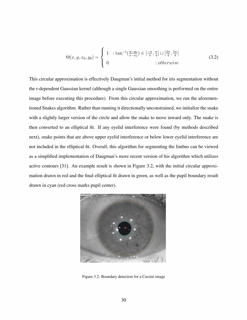
This circular approximation is effectively Daugman’s initial method for iris segmentation without

the r-dependent Gaussian kernel (although a single Gaussian smoothing is performed on the entire

image before executing this procedure). From this circular approximation, we run the aforemen-

tioned Snakes algorithm. Rather than running it directionally unconstrained, we initialize the snake

with a slightly larger version of the circle and allow the snake to move inward only. The snake is

then converted to an elliptical fit. If any eyelid interference were found (by methods described

next), snake points that are above upper eyelid interference or below lower eyelid interference are

not included in the elliptical fit. Overall, this algorithm for segmenting the limbus can be viewed

as a simplified implementation of Daugman’s more recent version of his algorithm which utilizes

active contours [31]. An example result is shown in Figure 3.2, with the initial circular approxi-

mation drawn in red and the final elliptical fit drawn in green, as well as the pupil boundary result

drawn in cyan (red cross marks pupil center).

Figure 3.2: Boundary detection for a Cassini image

30

Often, images taken at a diagnostic device have some degree of eyelid interference concealing a

portion of the iris. To mask out these regions from consideration in the registration algorithm,

eyelid/iris boundaries must be segmented. To this end, a Difference-Of-Gaussians (DOG) filter is

applied, which has been empirically parameterized to remove eyelid/iris boundaries from the image

(i.e. the area containing the boundary becomes dark) without removing the majority of the other

features from the image. The image is then converted to an inverted binary image – all pixels below

a certain threshold are made white, and all other pixels are made black. The resulting image has a

very thick white edge representing the eyelid interference with the iris, as well as some extraneous

smaller white edges throughout the iris. These extraneous edges are then filtered out by a novel

algorithm utilizing the integral image concept. The underlying concept is similar to the classical

“erode” algorithm that is often used for getting rid of small extraneous clusters of edges, with

the difference being that the average intensity in the “neighborhood” of a white pixel determines

whether it is kept or removed, as opposed to the amount of its neighbors that are white making

the determination. The “neighborhood” is shaped as a horizontal rectangle with an aspect ratio

of approximately 2, which is a decent enough match for the shape of typical eyelid interference.

This method allows for the small extraneous clusters of pixels to be removed without removing

any pixels belonging to the eyelid/iris edge. Had the classical erode algorithm been used instead, it

would have been very difficult to find a threshold that always gets rid of extraneous pixels without

also getting rid of the eyelid/iris edge. Classical erosion is still applied after the novel algorithm to

thin out the eyelid edge a little bit, but the key is that the novel algorithm allowed for a decoupling

of removing small clusters of extraneous pixels from thinning out all pixel clusters globally. After

this filtering, a bottom-up filter is applied to the upper eyelid region and a top-down filter to the

lower eyelid region, and a RANSAC circle finding algorithm is used on the resulting image to

extract the best circle for each eyelid. If RANSAC is unable to find a curve containing at least

an empirically determined number of pixels, it is assumed that there is no (or negligible) eyelid

interference. Figure 3.3 demonstrates the full procedure for eyelid detection, and Figure 3.4 shows

31

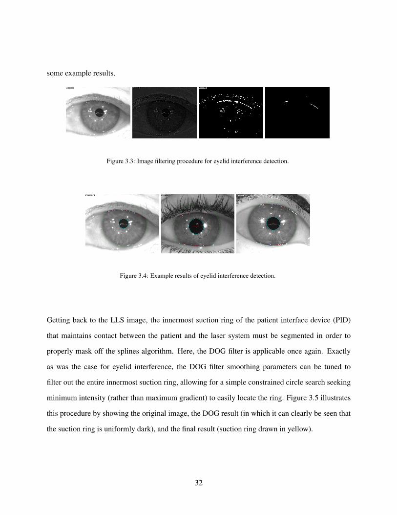
some example results.

Figure 3.3: Image filtering procedure for eyelid interference detection.

Figure 3.4: Example results of eyelid interference detection.

Getting back to the LLS image, the innermost suction ring of the patient interface device (PID)

that maintains contact between the patient and the laser system must be segmented in order to

properly mask off the splines algorithm. Here, the DOG filter is applicable once again. Exactly

as was the case for eyelid interference, the DOG filter smoothing parameters can be tuned to

filter out the entire innermost suction ring, allowing for a simple constrained circle search seeking

minimum intensity (rather than maximum gradient) to easily locate the ring. Figure 3.5 illustrates

this procedure by showing the original image, the DOG result (in which it can clearly be seen that

the suction ring is uniformly dark), and the final result (suction ring drawn in yellow).

32

Figure 3.5: Locating the innermost suction ring in an LLS image.

Filtering and Unwrapping the Iris

The iris during dilation is approximated by a rubber sheet model, such that the iris in the non-

dilated eye is assumed to basically be a stretched out version of the iris in the dilated eye. In this

approximation, a pseudopolar mapping is carried out to unwrap the iris into a rectangular image in

which the dimensions represent angle and distance from the inner (pupil) boundary. If the boundary

detection is perfect, then the top row of this image will perfectly represent the pupil boundary and

the bottom row will perfectly represent the sclera boundary. The size of the averaging area used to

fill each pixel in the unwrapped image increases linearly as a function of distance from the pupil

center [83]. An additional minor point to the unwrapping in this application is that the LLS uses

a fluid-filled patient interface device for the laser treatment, meaning that on top of the patient’s

eye there is a suction ring assembly containing a fluid filled chamber with a flat piece of glass on

top. This changes the refraction between the iris and the camera, as the cornea in air focuses light

towards the optical center of the eye. It is not difficult to discern the impact this has using simple

ray tracing. Basically, when imaging the iris in air the cornea “hides” some of the most peripheral

parts of the iris and causes the resolution in the iris to slightly degrade towards the periphery,

33

whereas the flat glass and fluid with index of refraction approximately equal to that of the cornea

result in being able to see a little bit more of the iris with a constant resolution throughout the

iris. Exactly how much more of the iris (in terms of radial extent) can be seen with the fluid-filled

interface depends primarily on the radius of curvature of the cornea. For typical curvatures, about

94% to 96% of the radial iris extent seen under the fluid-filled interface is visible in air. Thus, when

unwrapping the LLS image the radii of the limbus boundary are assumed to be 96% of their actual

values.

After unwrapping, the images are filtered with a Difference-Of-Gaussians (DOG) technique, which

is also done as a part of Chernyak’s algorithm and is similar to a step in Wildes’s iris recognition

algorithm [27]. This technique simply involves subtracting a severely blurred version of the image

from a slightly blurred version of the image, which is in effect a band pass filter in the frequency

domain. After applying the DOG filter, the histograms of the two resulting images are made

to be mutually consistent by simply stretching the histogram for the LLS image across the full

bandwidth for 8-bit images (0-255) and then scaling the intensity values of the topographer image

such that the average intensity of pixels not blocked by an LED reflection is equal to the average

intensity of the LLS image. This histogram modification method takes full advantage of the fact

that the LLS image has no bright LED reflections (or put another way, the LLS image already has

a well-behaved histogram). The result is increased signal strength of the iris fibers. An example

unwrapped image pair with these filtering operations applied is shown in Figure 3.6.

34

Figure 3.6: Unwrapped, DOG filtered iris (LLS top, topographer bottom).

Feature Extraction

A feature vector is built for each unwrapped iris image, with the content of the feature vector

being derived from gradient information from the structure tensor and Gabor filters. Thus, the

components of the image feature vector are themselves “local” feature vectors with one Gabor

filter component and one structure tensor component, and each of these two components are vectors

themselves. The information extracted from the Gabor filter is a point in the complex plane which

is computed by convolving a 2D Gabor wavelet with an area of the iris, according to formula

(3) [84].

∫∫I(ρ, φ)e−iω(θ0−φ)e

−(r0−ρ)2

α2 e−(θ0−φ)

2

β2 ρdρdθ (3.3)

Where α, β, and ω are wavelet size and frequency parameters, (r0, θ0) is the point about which

the area of the iris being considered is centered, and I is the intensity value of the unwrapped iris

image at a given point. In discrete form, this equation is applied as follows in equations (4) and

35

(5).

Re =

[ θ+∑φ=θ−

r+∑ρ=r−

I(ρ, φ)cos(ω(φ− θ0))e−(r0−ρ)

2

α2 e−(θ0−φ)

2

β2

](3.4)

Im =

[ θ+∑φ=θ−

r+∑ρ=r−

I(ρ, φ)sin(ω(φ− θ0))e−(r0−ρ)

2

α2 e−(θ0−φ)

2

β2

](3.5)

Where θ−, θ+, r−, and r+ denote the boundaries of the shell-like region over which the computation

is done. For unwrapped images, φ becomes x, ρ becomes y, and the region is rectangular rather

than shell-like. This allows for a simple and computationally fast implementation, which is to set

r0 and θ0 to zero and fill a 2D array with values according to the above equations with the image

intensity values removed, for each the real part and imaginary part, and then convolve these 2D

arrays with the images. This yields, at every pixel of each image, a 2D vector with components

for the real and imaginary part of the result of centering a gabor filter on that pixel. This mirrors

Daugman’s approach, sans the step of building a binary iris code.

Similarly, the structure tensor is used to extract gradient information in the local neighborhood of

each pixel. The entries in the 2x2 matrix representing the structure tensor are filled by averaging the

derivative-based quantity over the entire neighborhood. Then, the eigenvalues and eigenvectors are

extracted from the resulting matrix. The eigenvectors and eigenvalues give the dominant gradient

direction and a measure of the strength of the gradient, respectively.

S(x, y) =

f 2x fxfy

fyfx f 2y

(3.6)

36

Measuring Correlation Strength

Consider the filtered, unwrapped LLS image I1 and the filtered, unwrapped topographer image I2.

We define an inner product for the structure part of the feature vectors of the two images given a

particular hypothesized angle of cyclotorsion δ and a radial shear function ξδ(x) (to allow room for

errors in boundary detection and the rubber sheet model approximation) as follows:

PS(I1, I2, δ) =1

NS

[∑x,y

−−→∇I1(x, y) ·

−−→∇I2(x+ δ, y + ξδ(x))

|−−→∇I1(x, y)||

−−→∇I2(x+ δ, y + ξδ(x))|

](3.7)

Similarly, we define an inner product for the Gabor wavelet part of the feature vectors as follows:

PG(I1, I2, δ) =1

NG

[∑x,y

−→G1(x, y) ·

−→G2(x+ δ, y + ξδ(x))

|−→G1(x, y)||

−→G2(x+ δ, y + ξδ(x))|

](3.8)

With−→Gm a 2D vector corresponding to the complex number that results from applying the Gabor

filter to image m at the point (x, y). Some (x, y) points are ignored either due to local saturation

or being too close to identified regions of eyelid interference or the image boundary (see, for

example, the very top and very bottom of the second image in Figure 6). Additionally, a percentile

based thresholding is done for both the gradient features and the Gabor features, such that only the

strongest (according to magnitude of the complex plane vector) Gabor features are kept and only

the strongest (according to value of the larger eigenvalue) gradient features are kept. Thus, for

each metric, the summation is taken only over values that are kept for that metric and normalized

to the number of such values. As was previously mentioned, to allow room for a little bit of errors

in boundary detection and/or the rubber sheet model itself, a small radial shear is allowed, and

computed as follows. At each angular location (x-coordinate) and cyclotorsion angle δ, scores are

computed for different values of a radial offset ξδ(x) (an offset applied to the y-coordinate) and

37

note is taken of which value of ξδ(x) (denoted here as ξ′δ(x)) gives the strongest correlation for the

radial registration line defined by x and δ. To enforce continuity of the shear for each cyclotorsion

angle δ, ξδ(x) is chosen according to the following weighted averaging function:

ξδ(x) =

x+w∑x′=x−w

S(x′, δ, ξ′

δ)ξ′

δ(x′)

x+w∑x′=x−w

S(x′, δ, ξ′δ)

(3.9)

S(x, δ, ξ) =N

(x)S P

(x)S (I1, I2, δ) +N

(x)G P

(x)G (I1, I2, δ)

N(x)S +N

(x)G

(3.10)

When doing this computation, w needs to be large enough to prevent ξδ(x) from being completely

chaotic but not so large as to ruin the whole point of allowing a varying radial offset. For example,

10o has been observed to work well. Once the function ξδ(x) is computed for each δ, the inner

products as defined in equations (7) and (8) can readily be computed.

A strong correlation corresponds to large values of both inner products. The domain of both

inner products is [−1,+1] - thus, the net correlation is based on the average of the two inner prod-

ucts. Over a range of ±18o, a reasonable biological limit for cyclotorsion (see [20]) and head tilt

variation, the net correlation is computed from the average of the two inner products.

C(δ) =PS(δ) + PG(δ)

2(3.11)

Figure 3.7 shows an example plot of the correlation measures (Gabor, structure, and the average of

the two) as a function of cyclotorsion angle. Importantly, the global maximum of the net correlation

is significantly higher than any other local maximum. Note that the net correlation curve shown in

the figure has been smoothed to make peak extraction easier.

38

Figure 3.7: Correlation measures as a function of proposed cyclotorsion angle.

Allowing the radial shear makes a significant improvement to the success rate of the algorithm, as

it allows the algorithm to tolerate errors (within reason) in boundary detection that don’t impact

the center of the unwrapping. For example, in a pupil-centered unwrapping (which is used in this

study) the shear allows for any sort of error in the segmentation of the limbus and limited types

of error in the segmentation of the pupil (i.e. errors that don’t impact the center, such as ellipse

radii). This is critically important not only because segmenting the limbus is more challenging

than segmenting the pupil in general, but also because the limbus is often partially occluded by

eyelids which renders part of the geometry of the limbus inherently unknowable. It should be noted

that using a large aperture size in the feature extraction stage also helps to allow the algorithm to

tolerate these same kinds of errors to an extent. However, in the experimental section, we show that

allowing a small radial shear does significantly improve the expected success rate of the algorithm.

This method of determining similarity between two irises is, in a sense, somewhere in between the

methods of Chernyak and Daugman. Choosing the cyclotorsion angle to be the one that maximizes

the inner product PS with the radial shear function as described is mathematically very similar to

39

starting from Chernyak’s algorithm but using a much larger number of features (minimal sector size

and multiple features per sector). Choosing the cyclotorsion angle to be the one that maximizes

the inner product PG is very similar to the Daugman approach for choosing the best matching iris

image from the database of registered persons, the only difference being the decision to maximize

the sum of dot products between the complex numbers resulting from the Gabor filter rather than

minimize the Hamming distance between binary iris codes resulting from the Gabor filter (see

[24]). In fact, earlier versions of this algorithm did use the Hamming distance, but it was exchanged

for the inner product PG to allow for a more straightforward way of combining it with the other

inner product PS .

Extracting and Applying the Angle of Cyclotorsion

The angle of cyclotorsion is the angle that produces the maximum correlation strength between

the extracted features, which corresponds to the global maximum of the red curve in Figure 3.7. A

relative confidence score τ is computed based on how strong the global maximum is relative to the

next highest local maximum, according to the following formula:

τ = 100 ∗ (1− 101−r) (3.12)

Where r is the ratio between the global maximum and the next largest local maximum present

in the correlation function after Gaussian smoothing. For example, in the smoothed correlation

function for the plot in Figure 3.7, the global maximum is at +7.5 degrees, and the next strongest

local maximum occurs at−10.0 degrees. The correlation strengths at these cyclotorsion angles are

0.718 and 0.159 respectively; hence r = 4.516 and the resulting score is 0.9997. Note that r = 1

(the case of two or more global maxima) produces a score of 0, r = 2 produces a score of 0.9,

40

and it is impossible to obtain a score larger than 1 or less than zero (because r is guaranteed to be

greater than or equal to 1), as is illustrated by Figure 3.8.

Figure 3.8: Confidence score function based on peak height ratio.

The relative confidence score is multiplied together with the correlation strength at the global max-

imum of the unsmoothed correlation function to obtain a final score which can be used to decide

whether the registration was successful or not based on an experimentally determined threshold

(see the experimental section). This constructs a confidence metric that is both dependent on the

absolute value of the correlation strength and the value of the correlation strength relative to the

next most convincing peak in the correlation function. It is important for the metric to depend

on both of these – one can imagine that if the two highest peaks were of the exact same height it

would certainly not be sensible to arbitrarily pick one. Similarly, regardless of the relative score, an

absolute correlation strength significantly less than that of all image pairs verified to be correctly

registered should not be trusted.

In the left-handed natural coordinate system of the images, the cyclotorsion angle computed tells

what value of angle in the topographer image was lined up with the zero angle in the LLS image.

41

In the right-handed coordinate system (where counter clockwise corresponds to positive values of

theta), this is equivalent to how the topographer image would be rotated to line up with the LLS

image. This is the number needed, because treatment was planned in the frame of reference of the

topographer image.

The algorithm has been implemented in C++. In this implementation, the total run time for all

steps of the algorithm is on the order of 2 seconds on a modern desktop computer with an Intel

i7 processor. As the alignment is only done once (just prior to initiating the treatment), the time

added by doing the alignment is negligible.

Data Collection and Validation

The data required for input to the algorithm are two images of the same eye: one from a preop-

erative diagnostic device and one from a surgical laser. As mentioned in a prior section, the data

discussed at length in this paper came from the Cassini topographer (i-Optics) and the LENSAR

laser system (LLS). Initial development data were available for 10 eyes of 10 volunteer LENSAR

employees who were imaged at both devices without having surgery. The main validation of the

algorithms has been done using data for 50 eyes of 40 patients that underwent cataract surgery with

the LLS following a preoperative examination with the Cassini topographer. The image pairs for

this set of 50 eyes were acquired by a single surgeon as part of his standard operating procedures,

and the surgeon graciously sent the image pairs to LENSAR to be used in offline testing of the iris

registration algorithm (see the Acknowledgements section). As such, the only inclusion/exclusion

criteria to speak of is that the patients had cataracts. Due to the random nature of the sample, a

reasonable variation in eye color was observed over the 50 eyes, with noticeable variation in the

appearance of iris patterns in the infrared images that comprise the actual input to the algorithm.

42

Since the images were provided "as is" from a regular surgery context, there was no invasive

marking of any kind on the eyes to assist in validation; in fact, the fluid filled patient interface

device on the LENSAR laser would have frustrated any attempt to do so. Therefore, the only way

for the algorithm to be validated on this data set is through analysis of the iris patterns for matching

eyes. In many cases, due to the difference in pupil dilation between the two images and the impact

this has on the movement of iris features, it is extremely difficult for a human to perform a manual

registration completely independent of the algorithm. This limits the testing of the algorithm’s

correctness to manual verification (as opposed to manual validation) and statistical arguments. In

the manual verification process, trained human volunteers examine the output of the algorithm as

shown in Figure 3.9 and identify point correspondences (such as crypts or distinct fibers) in these

unwrapped and filtered images. The algorithm output highlights the section within each quadrant

of the iris that had the highest correlation, in order to reveal what the algorithm "saw" that led to

its decision.

Figure 3.9: Example registration result with highlighted matching sections.

A simple MATLAB program was used to display the images and compute cyclotorsion angles

from the feature correspondences, which are indicated by the volunteers with mouse clicks. The

volunteers were instructed to identify at least two and up to five point correspondences in each im-

age pair. The average cyclotorsion from all point correspondences identified by a volunteer for a

43

particular image pair is the cyclotorsion of the eye shown in the image pair as measured by that vol-

unteer. For each image pair, the "true shift" was defined as the average cyclotorsion taken over all

volunteers. A panel of three volunteers participated in this verification exercise. The standard de-

viation across the three volunteers, averaged over all 50 eyes, was 0.836◦, yielding a 95% tolerance

interval of ±1.67◦ for manual measurements. The average difference between the shift identified

by the algorithm and the true shift was 0.512◦ with a standard deviation of 0.422◦ (maximum of

1.75◦), yielding a 95% tolerance interval of ±1.36◦ for the algorithm’s measurements. Hence, the

95% tolerance interval of the algorithm is a tighter interval than that of the manual measurements.

Indeed, for each individual volunteer, the average difference between the shift identified by that

volunteer and the true shift was higher than that for the algorithm (0.57◦, 0.60◦, and 0.67◦) with a

standard deviation that was also higher than that for the algorithm (0.50◦, 0.47◦, and 0.56◦). Hence,

the 95% tolerance intervals for each individual volunteer were ±1.56◦,±1.54◦, and ±1.79◦, com-

pared with ±1.36◦ for the algorithm. Therefore, we can be 95% confident that the cyclotorsional

shift computed by the algorithm is within 1.36◦ of the true shift as defined above, and we can be

virtually certain that it is within 3◦ of the true shift (an error greater than 3◦ would be more than

6 standard deviations away from the mean). These results are summarized in Table 3.1 (all errors

defined relative to the true shift as defined above).

Table 3.1: Summary of manual validation results.

Registration Method Algorithm Manual 1 Manual 2 Manual 3

Average Error 0.512◦ 0.57◦ 0.60◦ 0.67◦

Standard Deviation 0.422◦ 0.50◦ 0.47◦ 0.56◦

95% Confidence 1.36◦ 1.56◦ 1.54◦ 1.79◦

As an independent statistical argument for correctness of the algorithm, the algorithm was allowed

to measure the correlation strength for every rotation angle in half degree increments from−180◦ to

44

+180◦, even though the correct answer in all cases is known to be within the range of−18◦ to +18◦

due to biological limits of cyclotorsion. For all 50 image pairs, the global maximum within the

range of−18◦ to +18◦ was equivalent to the global maximum within the range of−180◦ to +180◦.

A couple of examples are shown in Figure 3.10. This is a strong argument that the correlation

strength as defined in equation (11) is a reliable measure of similarity between two unwrapped iris

images, as it identifies in every case one cyclotorsion angle which measures superior to all others

and is always within the small set of physically possible cyclotorsion angles. Given this and the

results of manual verification, it is very difficult to imagine the algorithm being off by more than a

couple of degrees from the correct answer in any of the 50 image pairs examined.

45

Figure 3.10: Correlation plots extended to ±180 degrees.

Examining Figure 3.9, it is important to note that several locations the behavior of the iris under

dilation can readily be observed to be somewhat nonlinear – see, for example, how the tall dark

spot immediately to the right of the yellow rectangular boundary shifts in shape a little bit be-

tween images. This illustrates the nature of the registration under deformation problem and sheds

some light on why the algorithm used here is the right approach for this type of problem. Defor-

mation in this problem essentially corresponds to iris fibers between the two unwrapped images

changing slightly in length, shape, and/or orientation relative to the pupil boundary (hence here

46

we are only discussing the part of the deformation that is not accounted for by the rubber sheet

model). Small changes in length, shape, and orientation will in general cause small rotations of

the eigenvectors of the structure tensor, which is by no means drastic to a correlation based on the

inner product between these eigenvectors. These small deformations are also concentrated in the

domain of higher frequencies rather than lower frequencies, and Gabor wavelets extract informa-

tion from lower frequencies. Thus, both correlation metrics used here are theoretically capable of

handling small deformations in image registration. However, there is even more going on than just

deformation in this sense – places can also be identified where a feature present in one image is

completely absent in the other. For example, it is especially frequent for a group of small distinct

dark spots to “merge” into a single long dark spot under dilation (see the region between the cyan

and red rectangles). Occurrences like this indicate that an approach like Chernyak’s, which relies

on being able to pick out a small number of features and find their matching counterparts in the

other image, could struggle under pupil dilation (for reference, the eye giving rise to Figure 3.9

had pupil diameters of roughly 3mm preoperative and 6mm beneath the laser). It is also important

that the algorithm considers both high frequency and low frequency information, as in some cases

one provides a stronger registration signature than the other (see Figure 3.10).

When looking at the plots in Figure 3.10, it is tempting to believe that there is a fundamental limit

on how strong of a correlation can be obtained from an incorrect cyclotorsion angle. If such a limit

were to exist, it would assuredly be a safe acceptance/rejection threshold for the algorithm when

used in surgery. However, in the event that there are no data handling errors (i.e. the algorithm

is fed images of two different eyes to register), this threshold should be able to be made even

lower since the scoring method takes into account peak height ratios. In other words, if there are

no data handling errors, then the correct answer must be present, and thus if an incorrect peak is

chosen the peak corresponding to the correct answer should significantly damage the computed

confidence score, requiring a lower threshold to guarantee safety. This concept will be explored

47

further in the experimental section. However, for the current data set, it is always the case that the

global maximum in the extended correlation vs. cyclotorsion plot does correspond to the correct

answer.

Experiments

Impact of Pupil Dilation

Using a data set consisting of 50 eyes, some further analysis was done showing how varying pupil

dilation impacts the correlation strength. The most significant correlating factor was the difference

in pupil radius between the two images. Larger differences weakly correlate (R2 = 0.20) to lower

correlation strength of the registration, as shown in Figure 3.11. This provides strong evidence for

the theory that pupil dilation has in general a nonlinear impact on the movement of iris tissue.

Figure 3.11: Cyclotorsion-corrected correlation coefficient as a function of pupil size difference.

48

Efficacy of Masking Out Eyelids

Using a data set consisting of 50 eyes, results were compared between masking out eyelids and

not masking out eyelids. For the vast majority of cases, the difference in correlation value at the

correct cyclotorsion angle was insignificant (less than 0.05 for 45 out of 50 eyes, and less than 0.1

for 48 eyes), but for a few cases a significant decrease was observed when the eyelid masking was

disabled. For the most significant cases the amount of eyelid interference was especially severe.

It is to be expected that the majority of the time the algorithm does not need explicit protection

from eyelids, as masking out the pixels with lower feature strength for both Gabor and gradient

correlation methods often results in effectively masking out eyelids anyway (due to the low contrast

of eyelid skin).

Importance of Centration for Unwrapping

Accuracy and consistency of the center about which the iris is unwrapped is crucial to success of

the algorithm. It was discovered that the algorithm performs significantly better with the pupil

center used as the centration point as opposed to the limbus center. Using a data set consisting of

50 eyes, centering the unwrapping on the limbus decreased the correlation by 0.122 with a standard

deviation of 0.121 and a maximum decrease of 0.363. In terms of percent decrease in correlation,

the average was 19.0% with a standard deviation of 19.1% and a maximum decrease of 66.2%.

As a further experiment, the algorithm was run on each pair with the center of unwrapping shifted

vertically by 15 pixels from the pupil center for the diagnostic image. As expected, this severely

decreased the correlation. The average decrease was 0.131 with a standard deviation of 0.0860 and

a maximum decrease of 0.307. In terms of percent decrease in correlation, the average was 21.0%

with a standard deviation of 14.4% and a maximum decrease of 53.7%. In addition, the correlation

peak in the neighborhood of the correct cyclotorsion angle was observed to shift by as much as

49

4 degrees. It is easy to see why this effect is so drastic by considering how the polar mapping is

impacted by the centration error at different locations in the iris – angular locations of features

along the vertical axis of the eye are invariant to a vertical shift in the unwrapping center, whereas

angular locations of features along the original horizontal axis are not. Worse, the angular shifts of

features along the original horizontal axis are in opposite directions for features on opposite sides

of the center. Thus, a single torsion angle is no longer a sufficient description of the motion when

there is significant difference in the unwrapping center used between the two images. It is therefore

well understood why a deliberate induced centration error between the images causes such poor

performance. What is not as well understood is why a limbus centered unwrapping performs just

as poorly. It is true that in several cases, the limbus center cannot be known as accurately as the

pupil center due to eyelid interference in the topographer image. However, limbus centration is

observed to severely decrease the correlation even in cases without significant eyelid interference.

Further, the pupil center is not entirely static, as it can drift during dilation (such as when a circular

undilated pupil becomes an elliptical dilated pupil, or vice versa). It is therefore difficult to explain

the data without hypothesizing that the pupil center is biologically the most natural centration point

for obtaining a consistent polar mapping of iris tissue. This does not seem unreasonable - after all,

the pupil center only shifts as a result of physical movement of iris tissue, so it is not difficult to

imagine that if the iris gets stretched more intensely in a single direction than in the other directions

the rest of the iris gets pulled in that single direction along with the pupil center.

Radial Shear Efficacy and Error Rates

Experiments on radial shear (described in subsection 3 of section 3) are trickier to evaluate than

experiments on other parameters. This is because in varying the amount of freedom available to

the radial shear, the correlation is, in general, improved for incorrect cyclotorsion angles as well

as for correct cyclotorsion angles. Hence, there is an element of “trade-off” involved in evaluat-

50

ing different parameters for the radial shear function. Evaluating whether the “trade-off” yields

a net benefit requires assessing the ability of the algorithm to correctly decide which correlation

peak corresponds to the correct cyclotorsion angle. To make the evaluation, we took a statistical

approach as follows using a data set consisting of 50 eyes. For each radial shear amount tested

(in units of percentage of local pupil-to-limbus distance), the iris registration algorithm was run

on all 50 eyes in the set. In the resulting correlation versus cyclotorsion plot for each case, the

correlation at the peak corresponding to the correct cyclotorsion angle (which was the global max-

imum of the correlation plot in all cases) and the maximum noise level observed in the plot were

recorded. Here, maximum noise level is defined as the maximum correlation value not belonging

to the cyclotorsion peak in an extended range of -21 to +21 degrees. The reason for using the ex-

tended range with values at the boundary window counting as noise as opposed to only false peaks

counting as noise is that it results in a data set for max noise level that follows a normal distribution

and is assuredly a conservative quantity relative to the effective noise level when iris registration

is used in surgery. In the analysis that follows, we treat the correlation at the peak corresponding

to the correct cyclotorsion angle as "signal," and the max noise level as "background." The signal

and background statistics are presented in Table 3.2.

Table 3.2: Signal and background statistics for varying amounts of max radial shear.

Signal Max Background

Max Shear Allowed Min Max Mean Std. Dev. Min Max Mean Std. Dev.

0 0.351 0.777 0.556 0.102 0 0.315 0.117 0.077

10 0.426 0.846 0.620 0.098 0.065 0.383 0.169 0.077

20 0.462 0.843 0.627 0.097 0.064 0.388 0.192 0.076

40 0.378 0.833 0.598 0.102 0.062 0.411 0.190 0.080

The data clearly show that allowing any amount of radial shear results in an increase in both mean

51

signal and mean background. Therefore, this table on its own really does not provide enough

information as to which parameter set is best. In fact, this table doesn’t even appear to convey

whether any of the radial shear options perform superiorly to not having a radial shear at all. This is

where the statistics kick in. Seeing as how the right answer is still obtained in all cases, what needs

to be optimized is statistical predictability of this remaining the case on larger patient samples.

One important thing meant by predictability here is that we need to be able to set a threshold (as

described in section 3.5) for success, and we need to know that this threshold is high enough to

minimize the probability of a false positive (in which the algorithm finds a correlation satisfying

the threshold but it is actually just false background correlation) and to minimize the probability of

a false negative (in which the algorithm has found the correct answer but the correlation relative to

the detected background does not satisfy the threshold). One way to quantify the predictability is

by statistically evaluating the probability of the max noise level being higher than the correlation

value at the correct cyclotorsion angle (this is effectively a conservative estimate for the probability

of a false positive when the acceptance threshold is set to 0). When the correct cyclotorsion angle

is the global maximum of the correlation function, a false positive is impossible.

For each amount of max radial shear, we have the signal x and the max background level y mea-

sured for each patient. Both of these quantities fit well to normal distributions, as shown in Figure

3.12; using the Chi-squared test for normality, p > 0.93 for noise level and p > 0.99 for signal.

52

Figure 3.12: Correlation and max noise level measures are approximately normal.

Thus, for each radial shear parameter set, we have the means x, y and the standard deviations σx, σy

of the signal and max background level, and since more than 30 patients were used the squares of

the standard deviations are good approximations to the true variances as would be observed in an

arbitrarily large sample of patients [85]. The assumption of normal distributions allows us to place

53

conservative one-sided confidence intervals for the means according to the following formulas:

µx > x− zασx√n

(3.13)

µy < y − zασy√n

(3.14)

Where zα, 0.5 < α < 1 is given by the following formula using the standard normal distribution:

∫ zα

0

ns(x)dx = α− 1

2(3.15)

ns(x) =1√2πe−

x2

2 (3.16)

We want to estimate the probability that x − y > 0 for any x, y belonging to the normal distribu-

tions defined by (µx, σx) and (µy, σy) respectively. Note that this assumes complete independence

between signal and background, which appears to be a pretty good assumption for the patient sam-

ples used in this analysis based on a lack of correlation between signal and background. If they

are not independent, the current data predict that the relationship would be that of weak correlation

rather than weak anti-correlation (for all max radial shear amounts tested, linear regression on the

two variables yields anR2 value between 0.02 and 0.08), and in fact this is what would be expected

theoretically. After all, both signal and background are derived from the same correlation measure

with the only difference being whether the images are properly aligned or not, so when something

(such as the introduction of radial shear) increases the correlation measure in general, it results in

an increase in both signal and background. With this being the case, the assumption of indepen-

54

dence is remaining on the conservative side for showing x− y > 0 (since we are assuming a high

background level from one patient could have legitimately also wound up as the background level

for another patient which had a much lower signal, which is a false assumption if signal correlates

with background significantly enough).

To estimate the desired probability, we make use of both normal distributions:

nx(t) =1

σx√

2πe−

12( t−µxσx

)2 (3.17)

ny(t) =1

σy√

2πe− 1

2(t−µyσy

)2 (3.18)

We can compute the probability that y≈t0 by integrating the normal distribution for y over a small

neighborhood centered about t0.

P (y≈t0) =

∫ t0+δ2

t0− δ2

ny(t)dt≈δP (y = t0) (3.19)

We can also compute the probability that x < t0 by integrating the normal distribution for x from

negative infinity to t0.

P (x < t0) =

∫ t0

−∞nx(t)dt (3.20)

Finally, by integrating the product of these two probabilities over all values of t0, we obtain an

55

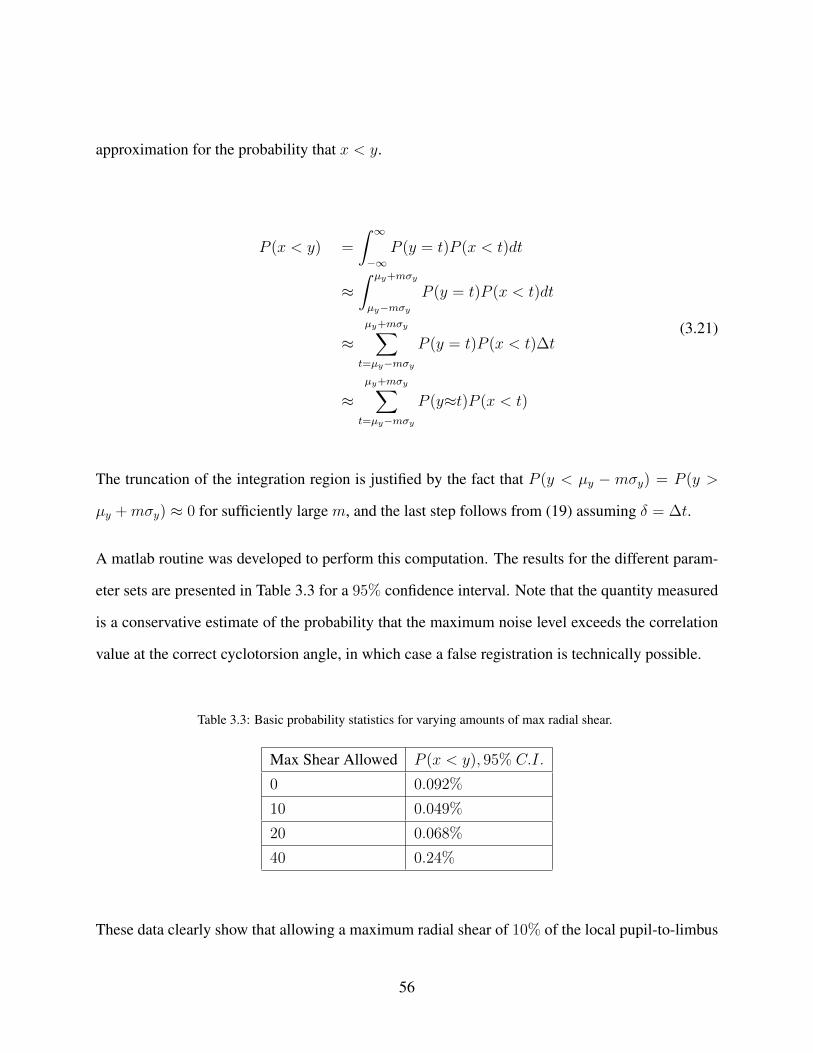
approximation for the probability that x < y.

P (x < y) =

∫ ∞−∞

P (y = t)P (x < t)dt

≈∫ µy+mσy

µy−mσyP (y = t)P (x < t)dt

≈µy+mσy∑t=µy−mσy

P (y = t)P (x < t)∆t

≈µy+mσy∑t=µy−mσy

P (y≈t)P (x < t)

(3.21)

The truncation of the integration region is justified by the fact that P (y < µy − mσy) = P (y >

µy +mσy) ≈ 0 for sufficiently large m, and the last step follows from (19) assuming δ = ∆t.

A matlab routine was developed to perform this computation. The results for the different param-

eter sets are presented in Table 3.3 for a 95% confidence interval. Note that the quantity measured

is a conservative estimate of the probability that the maximum noise level exceeds the correlation

value at the correct cyclotorsion angle, in which case a false registration is technically possible.

Table 3.3: Basic probability statistics for varying amounts of max radial shear.

Max Shear Allowed P (x < y), 95% C.I.

0 0.092%

10 0.049%

20 0.068%

40 0.24%

These data clearly show that allowing a maximum radial shear of 10% of the local pupil-to-limbus

56

distance results in better statistical predictability than all other shear limits tested (including no

shear at all). With this parameter set, we can be 95% confident that the chance of the maximum

noise level exceeding the correlation at the correct cyclotorsion angle is less than 0.049%. This

implies that with an acceptance threshold of 0, the false positive rate would be less than 0.049%,

since the maximum false correlation peak in the window of ±18 degrees (which is actually the

relevant quantity for how the algorithm operates in real surgeries) is guaranteed to be less than or

equal to maximum noise level as defined. The data also show that allowing too much radial shear

decreases the performance below that which would be obtained with no radial shear at all. Thus, a

“small” radial shear is best.

To connect one of the probabilities from the preceding discussion to a success/failure rate when

the acceptance threshold is taken into account, a small modification to the analysis is required. In

order for a false positive to be selected in the presence of a nonzero acceptance threshold, it is not

enough for the max background to have a higher correlation than that of the true signal (i.e. x < y).

Rather, the max background must also satisfy the following:

τ(y, x)y > T (3.22)

Where T is the threshold and τ(y, x) is the confidence scoring function given by

τ(y, x) = 1− 101− yx (3.23)

Note that τ(y, x) < 1, and if x < y then τ(y, x) > 0. With a little bit of algebra it is easy to show

57

that the relevant inequality for false positives (τ(y, x)y > T ) can be expressed as follows:

x <y

1− log10(1− Ty)) (3.24)

Notice that if T = 0 this reduces exactly to x < y. Thus, the exact same methods from the

preceding discussion apply perfectly in addressing this question under the simple transformation

below.

P (x < a)→ P (x <a

1− log10(1− Ty)≡ a′) (3.25)

Hence we can write the following.

P (τ(y, x)y > T ) ≈µy+mσy∑t=µy−mσy

P (y≈t)P (x < t′)

=

µy+mσy∑t=T

P (y≈t)P (x < t′)

(3.26)

The truncation on the lower end is justified by the fact that τ(y, x) < 1 implies that the inequality

can only hold if y > T . This yields the probability that the background correlation y corresponding

to a false peak is accepted despite the peak corresponding to the correct cyclotorsion value having

correlation x. Switching x with y yields the probability that the correct answer with correlation x

is accepted in light of background correlation y.

Using the established best radial shear limit of 10, a matlab routine was used to evaluate both prob-

ability quantities using the 95% confidence interval values for the mean signal and background.

58

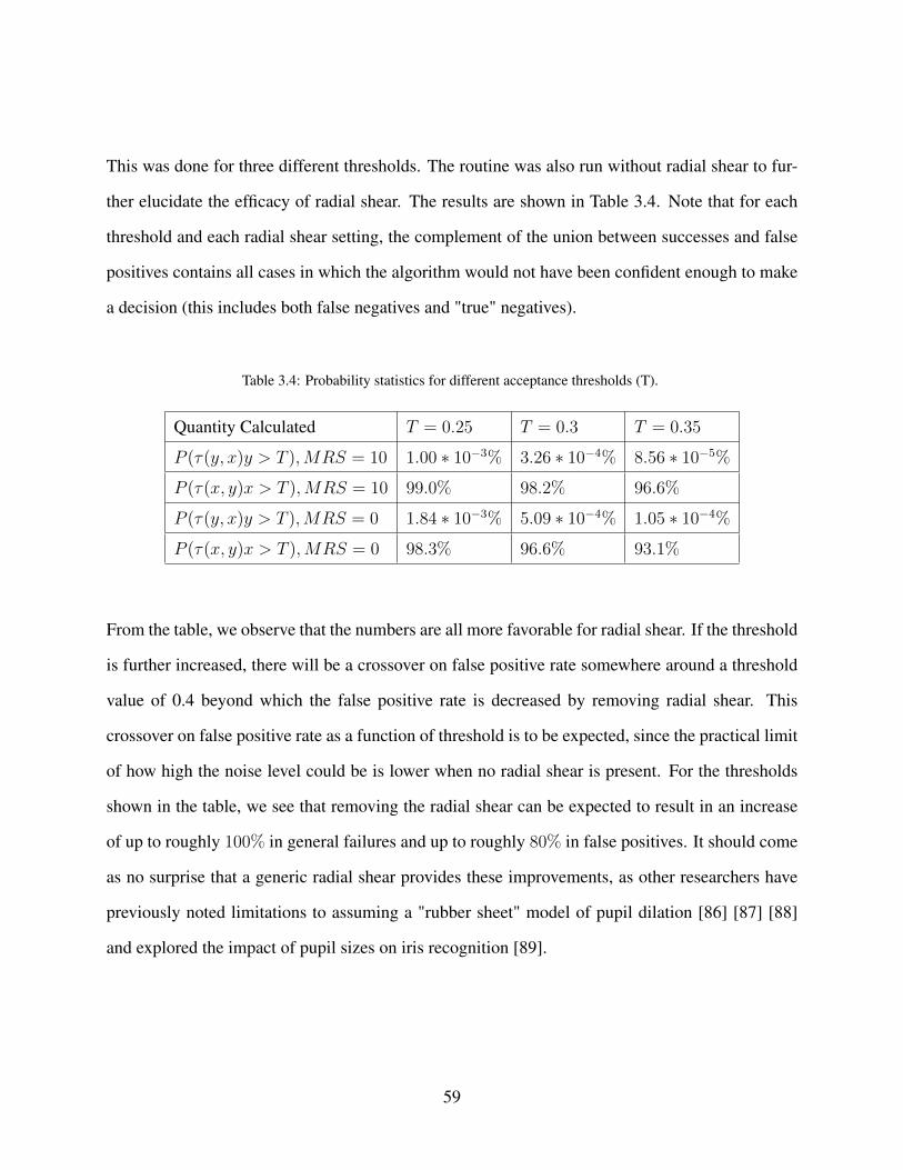
This was done for three different thresholds. The routine was also run without radial shear to fur-

ther elucidate the efficacy of radial shear. The results are shown in Table 3.4. Note that for each

threshold and each radial shear setting, the complement of the union between successes and false

positives contains all cases in which the algorithm would not have been confident enough to make

a decision (this includes both false negatives and "true" negatives).

Table 3.4: Probability statistics for different acceptance thresholds (T).

Quantity Calculated T = 0.25 T = 0.3 T = 0.35

P (τ(y, x)y > T ),MRS = 10 1.00 ∗ 10−3% 3.26 ∗ 10−4% 8.56 ∗ 10−5%

P (τ(x, y)x > T ),MRS = 10 99.0% 98.2% 96.6%

P (τ(y, x)y > T ),MRS = 0 1.84 ∗ 10−3% 5.09 ∗ 10−4% 1.05 ∗ 10−4%

P (τ(x, y)x > T ),MRS = 0 98.3% 96.6% 93.1%

From the table, we observe that the numbers are all more favorable for radial shear. If the threshold

is further increased, there will be a crossover on false positive rate somewhere around a threshold

value of 0.4 beyond which the false positive rate is decreased by removing radial shear. This

crossover on false positive rate as a function of threshold is to be expected, since the practical limit

of how high the noise level could be is lower when no radial shear is present. For the thresholds

shown in the table, we see that removing the radial shear can be expected to result in an increase

of up to roughly 100% in general failures and up to roughly 80% in false positives. It should come

as no surprise that a generic radial shear provides these improvements, as other researchers have

previously noted limitations to assuming a "rubber sheet" model of pupil dilation [86] [87] [88]

and explored the impact of pupil sizes on iris recognition [89].

59

Discussion

We have presented a solution to the problem of iris registration under both rigid and non-rigid

deformations for use in refractive cataract surgery, in which the large degree of pupil dilation is the

primary cause of non-rigid deformations. In stark contrast to previous work on iris registration, our

proposed algorithm does not rely on tracking feature correspondences. Instead, we have defined an

inner product between two unwrapped iris images using Gabor wavelets and the structure tensor,

which is computed for successive relative translations between the two unwrapped images under

the notion that the inner product should be maximized at the translation corresponding to the

cyclotorsional shift between the preoperative and intraoperative images of the eye. The inner

product includes a radial shear function to account for non-rigid deformations. We have also

presented a method of statistical analysis for the success rate of an iris registration algorithm,

which does not require any observed failures to be present in the data sample. We applied this

method to our algorithm using a sample size of 50 cataract patients and discussed how this method

could also be applied to other algorithms. Our proposed algorithm performed exceedingly well on

the data acquired – it was shown that when the algorithm is successful (which is the case with high

probability according to the statistical analysis), the computed cyclotorsion is accurate to within

two degrees with a high degree of confidence and is more reliable than a manual registration by

trained humans. Finally, we have highlighted the similarities between the related problems of iris

registration and iris recognition, in hopes of bridging these two research communities together

towards obtaining better understanding of the dynamics and mathematical structure of the human

iris.

Accounting for cyclotorsion is of paramount importance in any refractive surgery focused on cor-

recting and/or compensating for astigmatism. Although rotational misalignment is not the only

significant source of potential error in refractive treatments (for example, there are also challenges

60

associated with decentration relative to the preoperative measurement [90]), it is nevertheless ca-

pable of causing significant differences in refractive outcome if not accounted for. One interesting

challenge of applying iris registration to cataract surgery is the need to regularly operate over

large variations in pupil dilation. Although the rubber sheet model combined with the radial shear

method has proven to be sufficient for all data gathered so far, it is hoped that more data in this

context can lead to a better understanding of how the iris deforms under dilation. It may be that

further study of the radial shear function computed by the algorithm can shed some new insight on

the deformation. Regardless, the limitations of the rubber sheet model is a problem of interest to

the iris recognition community as well as the iris registration community, and therefore researchers

from both communities should continue searching for the best way to account for this. In addition

to proposing a new algorithm, we have also proposed a confidence scoring function to avoid unsta-

ble decision making and a statistical method for estimating the probabilities of false registrations

(or false positives) and successful registrations from a relatively small data sample (minimum sam-

ple size of 30, no requirement on number of successes versus number of false positives), both of

which should be applicable to iris recognition. In general, the application to iris recognition would

be straightforward: the confidence score (equation 12) for a recognition can be computed from the

two highest matches in the database, and for statistical analysis the signal could be defined as the

value of the match scoring metric for an authentic match with the background defined as the value

of match scoring metric for the best-matching imposter. In fact, these ideas could extend to other

recognition algorithms (such as face recognition) as well. The statistical analysis methods could

be particularly useful for the development of new algorithms since the amount of data required to

use the methods is not large. Interestingly, regarding prior work on iris registration, there doesn’t

appear to be any advanced statistical analysis of the performance documented. Chernyak [23] set

a threshold for the number of points used in the sinusoidal fit of torsion versus angular location

of features, but the threshold was just set as a little bit more than the largest number of points ob-

served when running the algorithm on pairs of images corresponding to different eyes. Under the

61

assumption that comparing different eyes is sufficiently similar to comparing images of the same

eye within a range of incorrect torsional alignments, this approach results in a false positive rate of

zero for the small sample studied but provides no indication of what the false positive rate might

actually be for an arbitrarily large sample. Since Chernyak’s algorithm doesn’t compute any kind

of “matching score” for any arbitrary cyclotorsion angle, it would not be quite as straightforward to

apply the statistical analysis methods described in this paper to it, but it could still be done using the

number of sinusoid points as the decision quantity – one would need a sample for approximating

a distribution of number of sinusoid points when the computed cyclotorsion is correct (to within

the intended accuracy), and a sample for when the computed cyclotorsion is incorrect. The latter

could perhaps be done by deliberately shifting one of the unwrapped images by an integer amount

of sectors (such that the correct feature matches cannot be found) for each sufficiently large inte-

ger, recording the greatest number of sinusoid points for any such integer, and repeating for each

image pair in the sample. A similar approach could be used for other torsion tracking algorithms,

although it might not be as important for applications that are not tied to surgical guidance.

Conclusion

This chapter presented our method for iris registration in its initial published form. Important

improvements and extensions have been made to this method since that time. The focus of these

is on the inclusion of a new free parameter in the registration: the center of unwrapping. The next

chapter describes the extension in terms of its motivation, method of operation, and efficacy.

62

CHAPTER 4: IRIS REGISTRATION WITH OPTIMIZED UNWRAPPING

Introduction

Iris registration refers to identifying significant transformation components between two images

of the same eye using the iris pattern. In surgical contexts, the major application is compensation

for cyclotorsion, which is a rotation of the eye within its socket when a person transitions between

sitting or standing (the position used for preoperative measurement) and lying down (the position

used for surgery) [20]. Further potential rotational misalignment exists in the form of variations in

how the patient’s head is presented to the different imaging systems involved. If unaccounted for,

rotational misalignment impacts astigmatism treatments, which must be aligned with the patient’s

axis of astigmatism for maximum benefit [22] [77] [79]. In the absence of automatic registra-

tion, the standard method for preventing rotational misalignment is to mark the eye with ink along

the nasal-temporal axis prior to surgery [22] [21], which limits alignment error to the difference

between the axis passing through the ink marks and the nasal-temporal axis as seen by the preop-

erative topographer.

In Chapter 3, we presented an iris registration algorithm that combined elements from successful

iris recognition algorithms with elements from previous work on iris registration, and demonstrated

highly effective performance on a set of 50 eyes imaged at both the i-Optics Cassini topographer

and the LENSAR Femtosecond Laser platform (abbreviated as LLS for LENSAR Laser System).

We also established that the pupil center was usually (although not always) a much better location

for centering the rotational registration than the limbus center. This raised an interesting question:

why should the pupil center be the ideal center of rotation for iris registration? What’s so special

about it? At the time, we hypothesized that the pupil center is biologically a much more natural

centration point than the limbus center, due to the fact that the movement of iris tissue is directly

63

responsible for changing the pupil center as the pupil dilates or constricts. We still believe there is

a lot of truth in this hypothesis, particularly when comparing the pupil center to the limbus center.

However, further study has now revealed that while the pupil center is superior to the limbus center,

unwrapping both images about the pupil center for the registration is still not optimal. If one of the

images is unwrapped about the pupil center, the optimal unwrapping center for the other image, in

terms of the merit function of the registration method, is generally not also the pupil center. The

optimal center can be found through gradient ascent on the merit function.

In this paper, we present a gradient ascent framework for optimizing the unwrapping center align-

ment for iris registration, using backpropagation to execute gradient ascent. This use of backprop-

agation is interesting in and of itself, as this technique is normally associated strictly with machine

learning methods such as neural networks. We also experimentally demonstrate the improvements

gained through this method, and explore whether there is any significance to the final unwrapping

center alignment itself. All experimental results were obtained using a substantially larger data set

than that used in Chapter 3. This expanded data set includes images from multiple topographers.

Method

The iris registration method in Chapter 3 identifies the rotational alignment angle between two

given iris images by maximizing a correlation function over the space of possible alignment angles

and radial shear. With the new gradient ascent step, the algorithm outline is the following:

1. Detect Pupil-Iris and Iris-Sclera boundaries in both images, as well as any eyelid interference

2. Filter and unwrap the iris in both images

3. Convert the unwrapped images from pixel representation to feature representation, where each

pixel gives rise to one feature vector

64

4. Measure global correlation strength between feature maps for each possible angle of cyclotor-

sion

5. Repeat steps 2-4 as required to optimize the unwrapping center in the laser image through gra-

dient ascent, maximizing the correlation strength at the global maximum.

6. Take the angle and unwrapping center with the strongest correlation and rotate the coordinate

system accordingly

The focus for this paper is step 5, which is the only step that was not present in Chapter 3. Figure

4.1 illustrates the original algorithm with intermediate image outputs, with the colored stripes in

the final images indicating the highest correlating section in each quadrant of the iris.

Figure 4.1: Visualization of the iris registration algorithm in Chapter 3.

Figure 4.2 shows how the algorithm is now embedded in a loop optimizing the unwrapping center

65

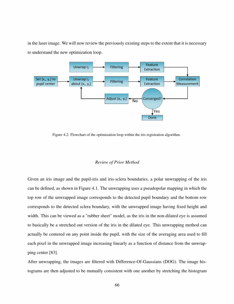
in the laser image. We will now review the previously existing steps to the extent that it is necessary

to understand the new optimization loop.

Figure 4.2: Flowchart of the optimization loop within the iris registration algorithm.

Review of Prior Method

Given an iris image and the pupil-iris and iris-sclera boundaries, a polar unwrapping of the iris

can be defined, as shown in Figure 4.1. The unwrapping uses a pseudopolar mapping in which the

top row of the unwrapped image corresponds to the detected pupil boundary and the bottom row

corresponds to the detected sclera boundary, with the unwrapped image having fixed height and

width. This can be viewed as a "rubber sheet" model, as the iris in the non-dilated eye is assumed

to basically be a stretched out version of the iris in the dilated eye. This unwrapping method can

actually be centered on any point inside the pupil, with the size of the averaging area used to fill

each pixel in the unwrapped image increasing linearly as a function of distance from the unwrap-

ping center [83].

After unwrapping, the images are filtered with Difference-Of-Gaussians (DOG). The image his-

tograms are then adjusted to be mutually consistent with one another by stretching the histogram

66

for the LLS image across the full bandwidth for 8-bit images (0-255) and then scaling the topogra-

pher image to render the average intensity of pixels not blocked by an LED reflection equal to the

average intensity of the LLS image.

A feature vector is built for each unwrapped iris image using a Gabor filter and the structure tensor.

This provides discriminatory information for the registration at every pixel of each unwrapped

image. The information extracted from the Gabor filter is a point in the complex plane which is

computed by convolving a 2D Gabor wavelet with an area of the iris [84]:

∫∫I(ρ, φ)e−iω(θ0−φ)e

−(r0−ρ)2

α2 e−(θ0−φ)

2

β2 ρdρdθ (4.1)

Where α, β, and ω are wavelet size and frequency parameters, (r0, θ0) is the location within the iris

that the computation is centered on, and I is the intensity value of the iris image at a given point.

In discrete form, this equation is applied as follows:

Re =

[ θ+∑φ=θ−

r+∑ρ=r−

I(ρ, φ)cos(ω(φ− θ0))e−(r0−ρ)

2

α2 e−(θ0−φ)

2

β2

](4.2)

Im =

[ θ+∑φ=θ−

r+∑ρ=r−

I(ρ, φ)sin(ω(φ− θ0))e−(r0−ρ)

2

α2 e−(θ0−φ)

2

β2

](4.3)

Where θ−, θ+, r−, and r+ denote the boundaries of the shell-like region over which the computation

is done. Since this operation is carried out on unwrapped images, the region becomes rectangular,

and the problem amounts to straightforward image convolution.

Similarly, the structure tensor is used to extract local gradient information at each pixel. The

quantities comprising the 2x2 structure tensor are averaged over the entire neighborhood, after

67

which eigenanalysis is executed on the resulting matrix. The resulting eigenvectors and eigenvalues

give the dominant gradient direction and a measure of the strength of the gradient, respectively.

S(x, y) =

f 2x fxfy

fyfx f 2y

(4.4)

From this extracted information, two inner products are defined between the unwrapped images I1

and I2. These are subsequently averaged to obtain the final correlation metric. The inner products

are defined for a particular hypothesized angle of cyclotorsion δ and a radial shear function ξδ(x)

(see Chapter 3 for more details) as follows:

PS(I1, I2, δ) =1

NS

[∑x,y

−−→∇I1(x, y) ·

−−→∇I2(x+ δ, y + ξδ(x))

|−−→∇I1(x, y)||

−−→∇I2(x+ δ, y + ξδ(x))|

](4.5)

PG(I1, I2, δ) =1

NG

[∑x,y

−→G1(x, y) ·

−→G2(x+ δ, y + ξδ(x))

|−→G1(x, y)||

−→G2(x+ δ, y + ξδ(x))|

](4.6)

C(δ) =PS(δ) + PG(δ)

2(4.7)

With−→Gm a 2D vector representing the complex number resulting from applying the Gabor filter

to image m at the point (x, y). Points that are too close to either eyelid interference or the image

boundary are ignored, as are points from areas of significant local saturation (such as LED reflec-

tions). There is also a percentile-based thresholding which results in the "weaker" features (based

on eigenvalue or Gabor magnitude) being ignored.

68

Optimizing the Unwrapping Center

The unwrapping method can be centered on any point inside the pupil. In our prior work, we

pointed out that it is very easy to see why changing the unwrapping center can significantly impact

the registration by considering what happens to the polar mappings. The most important result is

that the angular locations of features change, with the amount of change dependent on physical

location relative to the center. This is illustrated by Figure 4.3, which shows two features and their

angular locations with respect to two different points. In this particularly drastic example, the two

features change from being 180◦ apart to 210◦ apart. Thus, if one were trying to deduce a rotation

between polar unwrapped versions of these graphics, it would appear that the star rotated by −15◦

while the square rotated by +15◦, and so a single rotation angle where everything correlates well

simply does not exist. In contrast, if a consistent unwrapping center is used, everything correlates

perfectly at a rotation angle of zero.

Figure 4.3: Graphic demonstrating the effect of changing the unwrapping center on the angular location of features.

In the context of iris registration, it then becomes critical to have an optimized alignment of the

69

unwrapping centers between the two images. This can be achieved by leaving the unwrapping

center for one image fixed and optimizing the unwrapping center for the other image, seeking

to maximize the maximum correlation (assumed to correspond to the correct cyclotorsion angle).

Figure 4.4 shows an example surface plot of the maximum correlation as a function of the unwrap-

ping center of an LLS image, with the unwrapping center of the corresponding topographer image

fixed at the pupil center. Importantly, the peak containing the global maximum is fairly broad and

smooth, which means gradient ascent can ultimately be used to find the global maximum (and

thereby the ideal unwrapping center for the laser image). Of course, it is of critical importance that

gradient ascent starts from somewhere "on" the correct peak. This is ensured by testing out a few

additional unwrapping centers before launching into gradient ascent whenever the correlation at

the pupil center is significantly low. These additional "test unwrapping centers" are equally spaced

along the perimeter of a sizable circle centered on the pupil.

Figure 4.4: Surface plot of the registration correlation measure as a function of the LLS image unwrapping center

(relative to the pupil center).

Gradient ascent requires obtaining some approximation to the derivative of the correlation measure

with respect to both coordinates of the unwrapping center, and then updating the center as follows

(subsequently recomputing the max correlation value at the new center) until some convergence

70

criteria is satisfied:

xt+1c = xtc + ηt

dC∗

dxtc(4.8)

yt+1c = ytc + ηt

dC∗

dytc(4.9)

This update rule allows for the ascent rate η to decay following each iteration. Convergence can

be determined based on the magnitude of the derivative (the L2-norm is appropriate here since xc

and yc belong to a two-dimensional Euclidean space) and/or the raw increase in max correlation

(C∗) between successive steps. Of course, critical to this method is the question of how the deriva-

tives are calculated. One simple but effective method is to approximate the derivatives with finite

differences:

dC∗

dxc=C∗(xc + ∆)− C∗(xc)

∆(4.10)

dC∗

dyc=C∗(yc + ∆)− C∗(yc)

∆(4.11)

With an appropriate step size ∆, this method is extremely reliable. The obvious drawback is com-

putation time, as each derivative approximation requires redoing unwrapping, feature extraction,

and correlation measurement twice (once for each center coordinate). A better approach is to take

a page from the deep learning community’s book and use backpropagation to analytically compute

the derivatives. This amounts to repeated use of the chain rule, differentiating through each step of

the algorithm one at a time, starting with the computation of the correlation metric and going all

71

the way back through unwrapping. Importantly, an infinitesimal change to the unwrapping center

does not change the final registration transform (in this case, cyclotorsion and radial shear) or the

set of ignored points. This allows backpropagation to be implemented with the transform and the

set of ignored points being fixed at each iteration. More specifically, after each "forward pass" (i.e.

computing cyclotorsion and radial shear for a given unwrapping center), only the list of point pairs

that were used to compute the correlation metric need to be considered in the top-level derivatives.

These would be the derivatives of the correlation function with respect to the Gabor and Struc-

ture features (dC/d−−→∇I1 and dC/d

−→G1). Taking I1 to be the image having its unwrapping center

optimized (the laser image in this case), these top-level derivatives can be expressed as follows:

dC

dR1

=1

2

∂PG∂R1

=R2M

21 −M1M2R1

2NG(R21 +M2

1 )32 |−→G2|

(4.12)

dC

dM1

=1

2

∂PG∂M1

=M2R

21 −R1R2M1

2NG(R21 +M2

1 )32 |−→G2|

(4.13)

dC

dvx=

1

2

∂PS∂vx

=ux

2NS

(4.14)

dC

dvy=

1

2

∂PS∂vy

=uy

2NS

(4.15)

R and M denote real and imaginary (respectively) components of a Gabor feature in the image

indicated by the subscript, with−−→∇I1 ≡ (vx, vy) and

−−→∇I2 ≡ (ux, uy) (note these are the struc-

ture tensor eigenvectors, which are computed as unit vectors). As mentioned, these quantities are

evaluated for every pixel pair used to compute the last correlation value.

72

These derivatives then need to be backpropagated through feature extraction, the difference-of-

Gaussians filtering, and the image unwrapping. The necessary analytical derivative expressions

are all straightforward, but some of them are quite involved. For example, each component of the

normalized eigenvectors (vx, vy) needs to be differentiated with each of the three unique struc-

ture tensor elements (local second-order partial derivatives averaged over a neighborhood). As an

example, defining a ≡ f 2x , b ≡ fxfy, d ≡ f 2

y , and the discriminant of the eigenvalue equation

D = (a+ d)2 − 4(ad− b)2, two out of these six equations are the following:

dvxda

=b(λ− a)

2(b2 + (λ− a)2)32

(1− a− d

2√D

)(4.16)

dvyda

=b2

2(b2 + (λ− a)2)32

(a− d2√D− 1

)(4.17)

Through the chain rule, these are then used to arrive at derivatives of the correlation metric with

respect to each structure tensor element at each pixel:

dC

da=dC

dvx

dvxda

+dC

dvy

dvyda

(4.18)

The equations for this particular step are identical for the other two elements. The next steps are

the first ones to require using more pixels than just those involved in the final step, as the fea-

tures were extracted using neighborhood calculations. For each of the pixel locations containing

nonzero derivatives for the aforementioned quantities (which, to this point, can be managed in a list

rather than a two dimensional array), its local neighborhood must be looped through, incrementing

the derivative of the correlation metric with respect to each pixel in the unwrapped, DOG-filtered

image in accordance with how that pixel contributed to feature extraction at the center of the neigh-

73

borhood. In the case of the Gabor features, with GR and GM the real and imaginary components

(respectively) of the Gabor filter, the update rule is the following for pixels in a neighborhood

centered on (x, y):

dC

dF (x+ x′, y + y′)=

dC

dF (x+ x′, y + y′)

+GR(x′, y′)dC

dR1(x, y)

+GM(x′, y′)dC

dM1(x, y)

(4.19)

There are actually multiple update rules for the Structure tensor features, depending on how many

terms are used in the finite difference calculations of the local second-order partial derivatives

comprising the tensor. For two-term finite differences with a neighborhood of N pixels, the largest

update rule is the following:

dC

dF (x+ x′, y + y′)=

dC

dF (x+ x′, y + y′)

+1

N2fx(x

′, y′)dC

da(x, y)

+1

N2fy(x

′, y′)dC

dd(x, y)

+1

N(fx(x

′, y′) + fy(x′, y′))

dC

db(x, y)

(4.20)

There are also two similar update rules at (x + x′, y + y′ − 1) (which only affects b and d) and

(x+ x′ − 1, y + y′) (which only affects a and b). From here, difference-of-Gaussians can be back-

propagated through by simply applying the exact same DOG filter to dC/dF , to yield the derivative

74

with respect to the original unwrapped image dC/dU . In order to discuss the unwrapping step, a

slight change in notation is necessary. To this point we have been using x and y in discussing the

unwrapped images for clarity and convenience. However, now we need to use x and y to refer to

pixels in the original image, and so we will use θ and r to refer to pixels in the unwrapped image.

We sincerely apologize if this causes any confusion to the reader.

The formation of the unwrapped image U(θ, r) from the original image O(x, y) can be expressed

in the following generalized form:

U(θ, r) =

∑x,y

w(x, y, θ, r)O(x, y)∑x,y

w(x, y, θ, r)(4.21)

In other words, each pixel from the unwrapped image is formed from a weighted average of pixels

from the original image. In the normal log-polar sampling procedure, the weights are all either

zero or one, based on whether the pixel from the original image is inside or outside of the polar

sampling circle corresponding to the pixel in the unwrapped image. For iris registration, each

sampling circle, defined by center (sx, sy) and radius sr, is defined from the unwrapping center

and polar representations of the pupil and limbus boundaries (P (θ) and L(θ)) about that center, as

follows (note r is defined as the relative radial location of a point within the iris, such that r = 0

refers to the pupil and r = 1 refers to the limbus):

sx(θ, r) = xc + (P (θ) + (L(θ)− P (θ))r)cosθ (4.22)

sy(θ, r) = yc + (P (θ) + (L(θ)− P (θ))r)sinθ (4.23)

75

sr(θ, r) = k√

(sx(θ, r)− xc)2 + (sy(θ, r)− yc)2 (4.24)

However, if the weights are all either zero or one, this implies that the derivatives of the weights

are all zero, which would stop the backpropagation dead in its tracks. One can instead have the

weights linearly decay from 1 to 0 over some range near the boundaries of the sampling circles,

which creates a region of nonzero derivatives. Interestingly, one does not actually have to unwrap

the images with this more continuous scheme; the scheme itself is a (very good) approximation to

the normal in-or-out approach, and so it is perfectly valid to use the continuous scheme only for

computing derivatives. We have actually found this to be slightly superior to using the continuous

scheme across the board, both in terms of speed and efficacy. At any rate, the backpropagation

chain is completed by the following:

∂U(θ, r)

∂w(x′, y′)=

(O(x′, y′)

∑w(x, y)−

∑w(x, y)O(x, y)

)(∑

w(x, y)

)2 (4.25)

dw

dxc=

(∂w

∂sx+∂w

∂sr

∂sr∂sx

)(∂sx∂xc

+∂sx∂P

∂P

∂xc+∂sx∂L

∂L

∂xc

)+

(∂w

∂sy+∂w

∂sr

∂sr∂sy

)(∂sy∂xc

+∂sy∂P

∂P

∂xc+∂sy∂L

∂L

∂xc

)+∂w

∂sr

∂sr∂xc

(4.26)

The latter equation (for which there is another similar equation for yc) involves a lot of terms

which are all straightforward to compute, the lone exceptions being the derivatives of the pupil

and limbus boundary representations. These are instead computed using finite differences, using

76

a fast procedure for reparameterizing a closed curve in polar coordinates about a different center

which is not too far from the current center. At each θ, a line is projected from the new center in

that direction and the point from the previous representation closest to that line is found. r(θ) is

then set to the distance from the new center to that point, which assumes local circularity of the

boundary.

Experiments

Deidentified images of patients from the LLS and multiple preoperative devices were available for

experimental work. Some of this data were acquired by LENSAR for use in FDA submissions

for iris registration with each of the devices, and some were provided to LENSAR by surgery

centers post approval for algorithm testing and development. The preoperative devices and sample

sizes used for experimental work in this paper are as follows: the Cassini topographer (i-Optics,

N = 182), the OPD-Scan III (Nidek, N = 97), the Pentacam HR (Oculus, N = 151), and the

Pentacam AXL (Oculus, N = 77).

Registration Efficacy

Optimizing the center of unwrapping increases the likelihood of successful iris registration by ob-

taining a registration alignment that produces higher correlations - sometimes dramatically higher.

Table 4.1 shows the absolute and relative increase in correlation for each data set. The optimal

offset to the unwrapping center is usually fairly small, but in some cases it is quite large. The

existence of such cases constitutes the principal benefit of optimizing the unwrapping center, as

these cases tend to be at risk of the algorithm failing to find a sufficiently confident registration.

77

Table 4.1: Correlation increases as a result of optimizing the unwrapping center.

Device Correlation Increase Relative Increase

Cassini 0.04± 0.05 (max 0.26) 0.07± 0.11 (max 0.51)

OPD-Scan III 0.05± 0.07 (max 0.34) 0.10± 0.14 (max 0.76)

Pentacam HR 0.08± 0.12 (max 0.56) 0.20± 0.43 (max 3.11)

Pentacam AXL 0.05± 0.05 (max 0.27) 0.09± 0.10 (max 0.50)

Chapter 3 outlined in detail a statistical analysis method for obtaining robust conservative estimates

of the success and failure rates of the registration algorithm. In this context, success is defined

by accurately identifying the angle of cyclotorsion with sufficient confidence for acceptance (the

accuracy was established using manual registrations performed by multiple trained humans), while

there are actually two types of failure: identifying an incorrect cyclotorsion angle with sufficient

confidence for acceptance, and lacking the confidence to output any cyclotorsion angle. These rates

were estimated by fitting key quantities derived from the correlation metric to normal distributions

and measuring overlaps between the distributions that correspond to specific types of events. The

quantities are the correlation at the correct cyclotorsion angle (which we defined as signal, denoted

as x) and the highest correlation not on the peak containing the correct cyclotorsion angle (which

we defined as background, denoted as y). Normal distributions of these two quantities can be

used to estimate the probability that the signal is large enough to be accepted over the background

(P (τ(x, y)x > T )) and the probability that the background is large enough to be accepted over

the signal (P (τ(y, x)y > T )), where τ is the relative confidence score function defined by the

78

following:

τ(x, y) = 1− 10(1−xy) (4.27)

This function protects the algorithm from accepting a cyclotorsion angle doesn’t correlate signifi-

cantly better than some other angle (i.e. the case where signal x is roughly equal to background y,

which results in τ ≈ 0). The full details on how to compute each of the aforementioned probabili-

ties from the normal distributions can be found in Chapter 3.

An adjustment to this method of analysis is required before it can be applied correctly when the

center of unwrapping is optimized through gradient ascent. Although the signal uniformly in-

creases as a result of optimizing the unwrapping center, there is a new type of risk that is intro-

duced. This is the possibility of gradient ascent leading the algorithm to climb the wrong peak,

and subsequently accept an incorrect cyclotorsion angle due to the increased correlation strength

obtained from gradient ascent. When this occurs, the accepted background peak is only compet-

ing with the highest observed signal value, which is (generally) less than the final signal value

that would be obtained if gradient ascent climbed the correct peak. Similarly, when the correct

peak is climbed, the signal is only competing with the highest observed background peak. Thus,

there are now 4 relevant variables instead of only 2: both signal and background, before and af-

ter peak climbing. Keeping notation consistent with our prior work, x denotes signal, y denotes

background, and we now define xGA and yGA to refer to each quantity after being maximized by

gradient ascent. However, normal operation of the algorithm does not identify yGA. This can in-

stead be obtained for data analysis purposes by forcing gradient ascent to start from the strongest

background angle. Once normal distributions are obtained for each of the 4 variables, the desired

probabilities are actually computed exactly the same way as before, but with different inputs. The

probability of accepting the correct cyclotorsion angle is P (τ(xGA, y)xGA > T ), while the proba-

79

Table 4.2: Conservative estimates of registration success rates, with a fixed false registration rate of 3× 10−5.

Device P (τ(x, y)x > T ) P (τ(xGA, y)xGA > T )Cassini 98.90% (T = 0.23) 99.74% (T = 0.22)OPD-Scan III 97.09% (T = 0.24) 98.54% (T = 0.25)Pentacam HR 83.14% (T = 0.39) 99.34% (T = 0.29)Pentacam AXL 99.55% (T = 0.17) 99.86% (T = 0.18)

bility of accepting an incorrect cyclotorsion angle is P (τ(yGA, x)yGA > T ). Table 4.2 shows the

success rates as computed with this methodology using 95% confidence intervals, with the proba-

bility of accepting an incorrect cyclotorsion angle fixed at 3× 10−5 for all cases. The table shows

success rates both with (third column) and without (second column) the unwrapping optimization

step, demonstrating that this step provides significant improvement across the board.

Upon looking at both tables, the curious reader will no doubt wonder why the benefits of the new

step are so much more profound on Pentacam HR data than on other devices. Large correlation

increases from unwrapping optimization stem from the optimal unwrapping center being far away

from the pupil center. Inspecting the handful of cases with large unwrapping offsets reveals that

most of them result from the eye’s gaze direction not being perfectly on axis. It makes sense that

an off-axis gaze results in a high deviation of the optimal unwrapping center, but it is not clear why

this occurred more frequently in one particular device than any other. The Pentacam HR data used

in this study only came from two surgery centers, so it could be that the technicians operating that

device at those sites were simply not as careful as they could have been to ensure proper fixation

of the patient.

80

Benefits of Backpropagation

As previously mentioned, backpropagation was utilized for a more efficient implementation of

the main optimization loop. The simple alternative to backpropagation is to use finite differences

to approximate derivatives. While the finite difference approach is much easier to implement,

the major drawback is that, if n parameters are being optimized, n forward passes through the

algorithm must be executed for derivative approximation at each step. In contrast, backpropagation

provides derivatives for all parameters as part of a single backward pass through the algorithm.

Importantly, a backward pass through an algorithm generally has the same or similar computational

complexity as the forward pass. Thus, if we let τ represent the amount of time required to execute

a forward pass, the complexity of each step in an optimization loop isO((n+1)τ) = O(nτ) for the

finite difference approach, compared with O(2τ) = O(τ) for backpropagation. This means that

if n = 1, finite difference is a fine choice, but for a large amount of parameters backpropagation

becomes necessary. Even in cases where n is larger than 1 but still "small," one would expect

backpropagation to be significantly faster. In this particular case, the parameters being optimized

consist only of the x and y coordinate of the center of unwrapping in one of the iris images. Thus,

n = 2, which is the bare minimum for which backpropagation can be expected to provide speedup

over finite difference during gradient ascent. The speedup for each step is theoretically expected

to be around 50%, since two forward passes are replaced with one backward pass in each step

(alongside the constant single forward pass to recompute the correlation metric after each center

update in either case). The actual speedup depends on how similar the computation time is between

the backward and forward passes; if the backward pass is slower, the speedup will be less than 50%,

and vice versa.

Experiments were performed to quantify the benefits of backpropagation over a finite difference

approach to optimization of the unwrapping center. These experiments were carried out in C++

81

on a 6-core Intel i7 processor (many parts of the registration algorithm are multithreaded). The

registration algorithm was run each image pair twice: once using finite differences to optimize the

unwrapping center, and once using backpropagation. Computation time metrics for each method

are shown in Table 4.3. The times are only measured for the optimization portion of the iris

registration algorithm, as this is the direct measure of the speedup efficacy of replacing finite

difference with backpropagation. The speedups exceed 50%, indicating that the backward pass is

more efficient than the forward pass in the implementation.

Table 4.3: Computation time benefits of backpropagation in iris registration.

Data set Cassini OPD III Pent. HR Pent. AXL

Base Optimization Time 1.15± 0.59 1.18± 0.61 1.24± 0.58 1.10± 0.47

Backprop Optimization Time 0.54± 0.24 0.56± 0.30 0.65± 0.43 0.62± 0.28

Base Num. Loops 2.53± 1.27 2.45± 1.24 2.54± 1.27 2.32± 0.89

Backprop Num. Loops 2.32± 0.85 2.42± 0.97 2.50± 0.98 2.48± 0.82

Total Speedup 115.0% 112.9% 89.4% 76.4%

Per-Loop Speedup 97.7% 110.2% 86.9% 88.2%

The fact that the average number of loops remained largely unchanged across the board highlights

that this is an extremely fair comparison, as it implies that the stepping scheme was tuned equally

well for both methods of gradient computation. In other words, nearly the exact same intermediate

unwrapping centers are visited regardless of approach, and the speed with which each step is

executed is very nearly the only thing that changes. This is further illustrated by Table 4.4, which

shows very little difference in the output quantities between the finite difference approach and

backpropagation. Together, these tables show that backpropagation provided a significant speedup

82

without any drawbacks.

Table 4.4: Differences in final outputs between finite difference and backpropagation.

Data set Cassini OPD III Pent. HR Pent. AXL

Correlation −0.01± 0.02 −0.01± 0.03 0.00± 0.04 −0.01± 0.02

Final center (µm) 57.5± 40.5 59.3± 55.6 65.0± 58.7 64.3± 36.7

Cyclotorsion (◦) 0.16± 0.25 0.17± 0.47 0.14± 0.56 0.12± 0.23

Significance of Final Unwrapping Center

We now examine whether there is any significance to the final unwrapping center obtained from

the gradient ascent procedure.

Our hypothesis is the following: if the topographer image is unwrapped about the pupil center,

then the optimal unwrapping center for the laser image is a very good approximation to the pupil

center as seen by the topographer. The most significant implication of this hypothesis is that, if the

topographer image is photopic, our iris registration procedure identifies the approximate location

of the photopic pupil center in the laser image, which is in general not equivalent to the pupil center

as would be measured in the laser image (because pupil can change shape when dilating). This

could have important implications for refractive surgery [90].

To investigate our hypothesis, we explored a realistic model of pupil dilation using image warping.

In attempting to model dilation, there are two obvious boundary conditions: the pupil boundary

expands, and the outer edge of the iris (near the limbus) remains unchanged. The most straightfor-

ward way to model dilation is then to move each point on the pupil boundary away from the pupil

83

center according to some continuous function of angle, and then interpolate this outward move-

ment across the iris, linearly decaying to zero movement at the limbus. This method produces

extremely realistic images. If this is an accurate representation of how pupil dilation occurs, our

hypothesis can be mathematically proven to be correct, provided there is no appreciable difference

in tilt or gaze direction between the two images. The reason this model would prove our hypothesis

is that every point within the iris moves along the line connecting it to the original pupil center,

rendering the original pupil center as the unique point that preserves the angular mapping of all iris

features. Some example images produced by this model are shown in Figure 4.5. The first image

is the original, with the other images generated by applying our model to this image with different

dilation transforms.

Figure 4.5: Example outputs of our static pupil dilation model.

Although the images produced by this dilation model look very realistic, it seems quite likely that a

more accurate model would be one that breaks the image warping into steps, with the pupil center

updated at each step, such that the pupil is always expanding outward from the current pupil center

rather than the original. Some example images produced by this more dynamic model are shown in

Figure 4.6. Once again, the first image is the original, with the other images artificially generated

using the model.

84

Figure 4.6: Example outputs of our dynamic pupil dilation model.

This more dynamic model removes the theoretical guarantee of our hypothesis, thus requiring

further testing. Within this new model, it is easy to show that the optimal unwrapping center shifts

by some amount in the opposite direction of pupil center drift. A particularly egregious example

is shown in Figure 4.7, using a simulated dilation that shifts the pupil center roughly 375 microns

from its initial location. The tiny shift in the angle-preserving unwrapping center can be seen by

looking at where the top-left and bottom-right LED reflections line up relative to the angle spokes

(zooming in may be required to see the difference). Even for this overly dramatic example, the

maximum angular shift is only about 1.5◦, and the angular shift decreases for points closer to the

axis of pupil center translation as well as points closer to the limbus. Having said that, the LED

reflections can be used to put an upper bound on how far away the optimal unwrapping center has

moved from the initial pupil center. A gradient descent procedure was run to find the unwrapping

center that minimized the sum of squared differences in angular locations of the centers of the

LED reflections between the images produced by both dilation models, with angles measured with

respect to the original unwrapping center for the first model and angles measured with respect to

the center being optimized for the second model. The optimal center was only 80 microns away

from the original center. This experiment was repeated with a pupil center shift of roughly 200

microns in a different direction, with the result that the optimal center was only 40 microns away

from the original center. These results suggest that, in the absence of significant tilt difference, the

85

distance between the optimal unwrapping center and the original pupil center is likely to be less

than 25% of the amount of pupil shift during dilation.

Figure 4.7: Comparison between the static (left) and dynamic (right) dilation models.

Conclusion

We have presented a robust extension to a previously published iris registration algorithm. The

extension is based on allowing the center of unwrapping to freely float within an optimization

loop in one of the images, rather than leaving it fixed on the pupil center for both. Superior

performance was experimentally demonstrated for the updated algorithm using data from multiple

devices. Experimental data was also presented showing that the final unwrapping center - which

is a new secondary output of the algorithm - has a large amount of invariance to dilation-driven

pupil center drift, and could therefore possibly serve as a reliable estimate of the photopic pupil

center under certain circumstances. Finally, backpropagation was utilized in the new algorithm

implementation, making this work a very interesting and unique application of a technique that is

normally associated strictly with machine learning.

Like nearly all prior work in iris registration and recognition, our registration method did not uti-

lize any machine learning (although the use of backpropagation was for sure inspired by research

in machine learning). In light of the high performance demonstrated with this method, it is fair

to wonder whether machine learning could ever have a place in this specific field. One certainly

86

would not be keen on completely scrapping an approach performing this well and starting from

scratch with a deep learning method. At the same time, the method contains several numerical

parameters that were set by hand. Many of these are in the segmentation step (edge thresholds,

kernel sizes for gradient estimation, difference-of-gaussian parameterization, etc.), along with a

few in feature extraction (Gabor wavelet parameters and difference-of-gaussian parameterization).

It would be naive in the truest sense to believe that every one of these parameters is fully optimized.

This leads to the interesting question of whether it is possible to embed any of these algorithms "as

is" into a machine learning approach such as a convolutional neural network (CNN) and achieve

this parameter optimization. In principle, one would even expect that additional parameters could

be utilized which are initialized as having no effect but then potentially "discovered" to be use-

ful. The next chapter takes a look at this question by embedding a RANSAC algorithm for pupil

segmentation into a CNN with a novel RANSAC-based loss function.

87

CHAPTER 5: IMPROVING RANSAC SEGMENTATION THROUGH

CNN ENCAPSULATION1

Introduction

Convolutional neural networks (CNN) have revolutionized the field of computer vision over the

course of the past few years. This recent revolution had its ultimate origins in the specific area of

object recognition in two-dimensional images, and then quickly spread to other areas such as se-

mantic segmentation. As part of the natural evolution of the methodology, early work on utilizing

CNNs for segmentation maintained as much similarity as possible to the successful object recog-

nition approaches. Among other things, this led to the still commonly used approach of training a

CNN to classify individual patches from images rather than operating on the entire image at once.

Recent works on segmentation [54] have begun to move away from this for a variety of reasons,

including efficiency. Indeed, the approach of operating on the entire image at once in CNN-based

segmentation bears much clearer resemblance to segmentation pipelines which do not involve deep

learning.

Model-specific segmentation problems, defined as a segmentation problem in which some straight-

forward mathematical form for the boundary of the desired object(s) is known beforehand, have

yet to be explored with CNNs to the extent that other segmentation problems have. One popular

approach to model-specific segmentation problems is to use RANSAC to enforce the mathematical

form, as this method is extremely robust to outliers. In these approaches, there are usually filtering

and thresholding steps that occur on the original input to generate the input for the RANSAC al-

1This content was reproduced from the following article: D. Morley and H. Foroosh, "Improving RANSAC Seg-mentation Through CNN Encapsulation," Proceedings of the IEEE conference on computer vision and pattern recog-nition, 2017. The copyright form for this article is included in the appendix.

88

gorithm, and these steps traditionally do not utilize machine learning for optimization. We seek to

demonstrate that these approaches (or at least significant pieces of them) can in general be directly

encapsulated into a CNN "as-is", and that upon doing so the parameters can be fine-tuned through

backpropagation using a novel error function which is directly tied to the propensity of RANSAC

to choose the true segmentation over any false segmentation. Another interesting aspect of do-

ing this is that a CNN constructed for a model-specific segmentation problem will generally be

significantly smaller than the CNN architectures currently participating in the modern deep learn-

ing revolution. Thus, our work offers some validation of how well CNN concepts and techniques

generalize to smaller problem sizes.

We apply our CNN formulation to the problem of pupil segmentation in images of human eyes.

This is a problem with important applications to biometric identification [84] [31] [27] and oph-

thalmic surgery [23] [1] that has been well-studied with classical computer vision approaches,

which are capable of achieving a very high success rate on this problem due to the contrast be-

tween the pupil and iris being quite good under normal infrared imaging conditions. The fact that

gradient strength is a key underlying assumption in these algorithms directly implies that it should

be possible to exchange parts of these algorithms for a CNN and achieve better performance. We

explore this directly by first constructing an algorithm along the lines of typical classical computer

vision approaches (specifically, a combination of thresholding, edge detection, and filtering out ex-

traneous edges), directly converting this algorithm into a CNN (by directly copying convolutional

filters, using combinations of filter biases and ReLU layers for thresholding, and adding custom

layers for additional calculations where necessary), and then executing training epochs to further

fine-tune the constructed CNN on a RANSAC loss function. Figure 5.1 shows this CNN structure

with idealized intermediate outputs for the problem of pupil segmentation.

89

Figure 5.1: Our method for improving RANSAC segmentation performance by CNN encapsulation.

In summary, our work makes the following contributions: we present a novel framework for

model-specific segmentation that unifies CNN and RANSAC approaches using a loss function

based on RANSAC outputs; we demonstrate success in using our framework to fine-tune a func-

tional RANSAC segmentation algorithm through CNN training; we demonstrate robustness of our

method through a multiplicity of experiments; and we demonstrate successful utilization of a CNN

for a problem type and size that is very different from typical CNN work, thus providing significant

90

additional validation of the adaptability and generalizability of the CNN framework.

Related Work

CNNs have been a topic of active research and discussion, particularly since significant perfor-

mance gains on image classification were first reported [47]. Although the fundamentals of the

CNN technique can be said to have already existed for a few decades [97], it has only been in re-

cent years that CPUs and GPUs have advanced far enough to allow these techniques to be applied

to large sets of typically sized images. Since this time, there have been important ongoing discus-

sions about topics like how trained CNNs can be interpreted [2] and how well they generalize to

other data sets or even different tasks [62]. CNNs have also been successfully applied to a variety

of vision tasks besides classification, such as segmentation [53] [54], super-resolution [61], and

edge detection [59].

An important concept that has come to light with CNNs in recent years is the idea of fine-tuning,

normally referring to the practice of taking as a starting point a CNN which has been pre-trained

for some task and data set and applying it to a different task and/or data set. Success in doing so is

well documented [59] [62], with the pre-trained nets having at least reasonable performance right

off the bat (due to the fact that filters within a pre-trained CNN exhibit positive responses to a large

variety of useful features) and fantastic performance following training. Our work slots into this

area in general, but with the important distinction of starting from a manually designed "simple"

CNN rather than a pre-trained deep CNN. We were unable to find any instances in the literature of

other researchers attempting this task.

Another interesting development in CNNs that has emerged with the variety of problems they are

being used to tackle is the utilization of a wide variety of loss functions for training. One example

91

of growing interest is the use of structured loss for precise locations of objects [100] [58]. As

another example, Shen et al. [60] proposed a unique loss function for contour detection based on

the idea that a false negative in contour detection is a more significant error than mislabeling the

"type" of contour. These examples demonstrate the importance of defining a loss function that

is aligned as closely as possible with the most important metrics for the problem at hand. This

philosophy is what inspired us to experiment with a unique RANSAC-based loss function (see

section 3.4) for a model-specific segmentation problem, as this allowed us to pinpoint the loss

function directly onto the success rate of the final emergent algorithm. This is in direct contrast to

typical CNN segmentation approaches in which object boundaries are not direct outputs and must

be found by applying additional algorithms to the CNN output (e.g. the CNN might output some

kind of probability map from which boundary information must be extracted via algorithms like

graph cut or RANSAC).

RANSAC [3] [101] has been applied to many different problems, ranging from robotics [4] [5] to

biomedical image processing [6] [7] [8] [9]. Its many advantages include robustness to outliers and

ease of implementation. However, like all estimation methods, its performance has dependence on

the input. If all inliers are present and there is no set of outliers forming a strong instance of the

model being fit to, RANSAC is virtually guaranteed to identify the correct model given enough

iterations. If some inliers are missing, RANSAC output can have accuracy issues. If there are

a lot of outliers present, or if a large subset of outliers just so happen to form a model instance,

RANSAC can experience a catastrophic failure of selecting a model formed from outliers rather

than inliers. Therefore, whenever RANSAC is in use, it is important to optimize the input as much

as possible. We seek to demonstrate that convolutional neural networks can be an effective tool for

accomplishing this optimization task.

92

Method

In this section we describe our approach in detail. Our CNN contains four phases: preprocessing,

feature extraction, clutter removal, and RANSAC model fitting. The first three phases all contain

convolutional kernel weights and biases that can be optimized through network training. The

weights and biases can also be initialized prior to training based on existing insights from other

successful approaches to the problem at hand. We would argue that the ease of initialization with

our approach makes it ideal for industrial applications where the algorithms currently being used

already perform very well, as this allows for a starting point that largely (if not entirely) preserves

the original performance prior to any machine learning. The final phase of our CNN is a RANSAC

layer, which performs straightforward RANSAC model fitting in the forward pass and computes a

novel RANSAC-based loss function in the backward pass.

Preprocessing

For the class of problems to which our method is applicable, the preprocessing phase can in-

volve any combination of smoothing, rescaling, and thresholding. In CNN terms, smoothing and

rescaling are convolutional operations, while thresholding can be performed by adding biases to

the kernel outputs and then passing the output through a rectified linear unit (ReLU) layer. The

significance of this phase has a lot of dependence on the regularity of the intensity profile of the

object to be segmented relative to that of the background throughout the data samples. For more

irregular intensity profiles, this layer would either have to be less aggressive, or include a sizable

multiplicity of kernel/bias combinations.

93

Feature Extraction

The goal of the feature extraction phase is to construct feature maps from the outputs of the pre-

processing phase. For a successful segmentation, the union of these outputs should ideally contain

the full set of boundary points for the object of interest, with the amount of false positives being

minimal and/or easily reduced by the clutter removal phase. The backbone of feature extraction

is ultimately a set of convolutional filters, with the main source of diversity in different feature

extraction methods lying in the set of filters used and the way in which their outputs are ultimately

combined. For example, edge features have directional dependence to them, meaning that a single

filter cannot capture all edges of an object. Therefore, a simple edge detection approach is to use

one filter to extract horizontal edge strength and one filter to extract vertical edge strength, and then

build a complete edge map from the Euclidean norm of the two resultant edge maps. To be sure,

this Euclidean normalization of two feature maps is not an operation traditionally found in CNNs,

but there is no reason why it couldn’t be given the appropriate context, as the euclidean norm is

indeed differentiable with respect to its inputs. We demonstrate successful application of this fact

in our experiments. In particular, we insert a custom layer into a CNN that performs the following

forward and backward calculations on two input channels denoted gx and gy given a loss function

L:

h =√g2x + g2y (5.1)

∂L

∂gx=∂L

∂h

∂h

∂gx=∂L

∂h

(gxh

)(5.2)

∂L

∂gy=∂L

∂h

∂h

∂gy=∂L

∂h

(gyh

)(5.3)

94

On the other hand, by utilizing more filters, one could just as well have a full bank of filters for

different edge orientations and combine them with one of several possible methods, including

Euclidean norm across all outputs, max across all outputs, average of all outputs, or another layer

of convolutional filters applied to the outputs (which collapses to the averaging option in the limit

that a single filter is used with the center value equal to 1 for all input channels and all other values

set to zero). Any differentiable operation is fair game in a CNN.

Clutter Removal

Once features have been extracted, it is often necessary to subject the features to some kind of

pruning process, consisting of any combination of throwing away weak features, removing certain

feature classes altogether, or successive application of additional filters to the feature maps. In a

CNN, ReLU layers are the most straightforward way to throw away weak features. Regarding the

other types of operations, a CNN can be constructed to have multiple largely independent channels

entering this phase, which is significant because it is then possible to interpret some of these chan-

nels as focused on obtaining high feature strength for boundary pixels of the object to be segmented

with the other channels instead focused on obtaining high feature strength for other objects or ar-

tifacts in the image. In this framework, some kind of weighted subtraction of the second kind of

channels from the first kind should yield a good final map for the desired object boundary. This idea

of a weighted subtraction can of course straightforwardly be executed with convolutional kernels,

which can simultaneously apply other interesting operations on the channels (such as smoothing)

prior to the subtraction. Alternatively, undesired objects or artifacts can also be filtered out ahead

of time in some cases. For example, many segmentation pipelines in iris recognition remove LED

reflections as one of the earliest steps [102] [103]. A CNN embodying this design philosophy is

simply one in which the first few layers produce an output which is (ideally) the original image

95

but with the undesired artifacts removed. We performed CNN experiments utilizing each of these

approaches to artifact removal (in fact, they are not mutually exclusive), but we focused more effort

on the first approach due to the implementation being much more straightforward.

RANSAC Fitting and Backpropagation

Perhaps the most unique aspect of our work is the novel RANSAC-based loss function we employ

in our CNN. RANSAC [3] [101] is a model fitting technique that is extremely robust to noise,

as outliers have no impact on the final shape provided the input has enough signal strength for

the desired shape. It is also an extremely generic technique, applicable to any modeling problem

where a fixed number of data points define an instance of the model. Our RANSAC implementation

for pupil detection operates directly on the output Z of the previous CNN layer according to the

following steps (assuming a circular model): construct a list of all points (x , y) where Z (x , y) > 0 ;

select three of these points at random and construct the unique circle C passing through these

points; compute a score for that circle based on the values of Z at points sufficiently close to the

circle, but assigning a score of 0 if the circle violates known geometric constraints; repeat the

random point sampling and circle scoring steps for a fixed number of iterations, maintaining (and

eventually returning) the highest scoring circle.

We now turn to a very interesting question: what causes RANSAC to fail? Certainly, if Z =

0 ∀(x , y) ∈ C ∗ with C ∗ denoting the true circle, RANSAC will surely fail. Indeed, the input

values at the points along the true circle are clearly a critical factor. But how high do these values

actually have to be? How low do the other values actually have to be? The answer is that if

the points satisfying the true model all have positive values, the only way RANSAC can actually

fail (assuming a sufficient number of iterations) to return the true model is if a more convincing

alternate model is present in the data. This means that not all false positives in Z are equally

96

important, as a set of false positives that don’t fit a single model instance (i.e. randomly scattered

points) are considerably less likely to cause issue than a set of false positives which do fit a model

instance. In the case of iris images, there are other structures present in the image besides the pupil

which form a circle: the eyelids, the outer iris boundary, and the ring of LEDs inside the pupil.

Thus, the key factor in whether RANSAC succeeds or fails provided decent representation of true

positives is the strength of the strongest "impostor" model instance. For this reason, we propose a

loss function centered on the ratio between the RANSAC scores of the strongest impostor and the

true model, together with additive terms to penalize false negatives and false positives (thus, the

error function completely ignores true negatives). Explicitly, our loss function is the following:

L = log

(1 + S

′

1 + S∗

)−α∑

(x,y)∈C∗Z(x,y)≤0

Z(x, y) + β∑

(x,y)/∈C∗∪C′

Z(x,y)>0

Z(x, y) (5.4)

With S′ and S ∗ the scores of the strongest impostor C ′ and the true model C ∗ respectively, with

scores computed by the following:

S =∑

(x,y)∈CZ(x,y)>0

Z(x, y) (5.5)

97

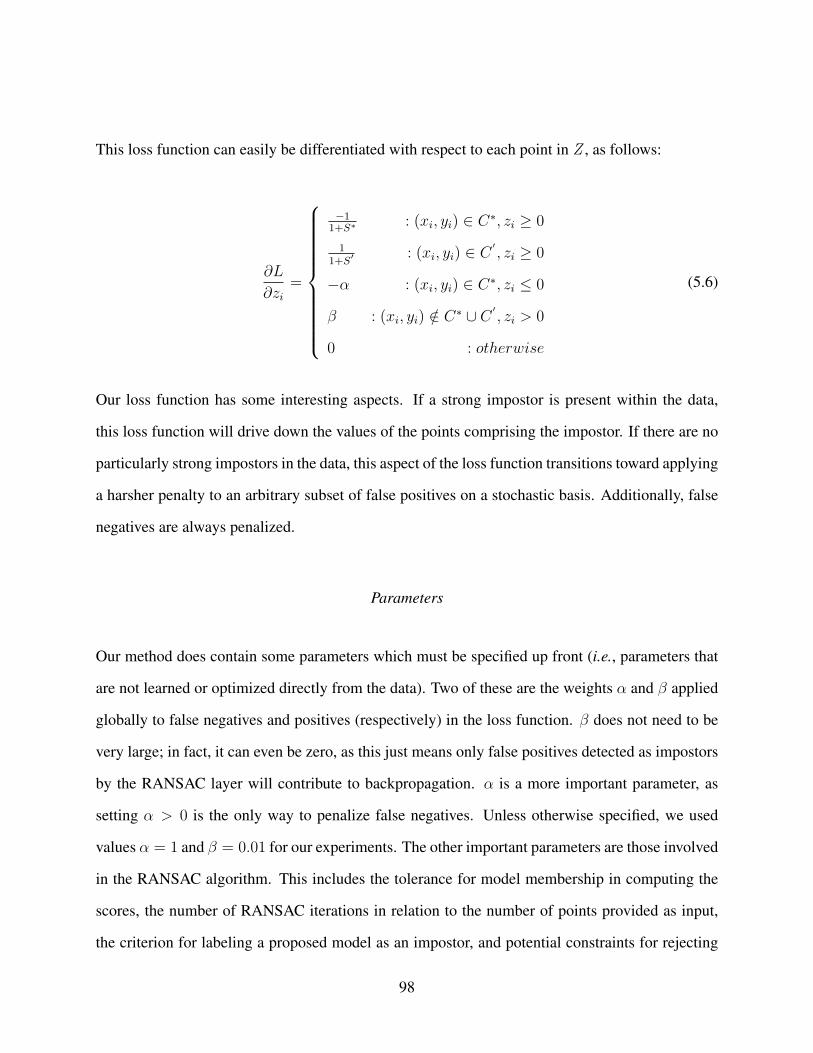
This loss function can easily be differentiated with respect to each point in Z , as follows:

∂L

∂zi=

−11+S∗

: (xi, yi) ∈ C∗, zi ≥ 0

11+S′

: (xi, yi) ∈ C′, zi ≥ 0

−α : (xi, yi) ∈ C∗, zi ≤ 0

β : (xi, yi) /∈ C∗ ∪ C′, zi > 0

0 : otherwise

(5.6)

Our loss function has some interesting aspects. If a strong impostor is present within the data,

this loss function will drive down the values of the points comprising the impostor. If there are no

particularly strong impostors in the data, this aspect of the loss function transitions toward applying

a harsher penalty to an arbitrary subset of false positives on a stochastic basis. Additionally, false

negatives are always penalized.

Parameters

Our method does contain some parameters which must be specified up front (i.e., parameters that

are not learned or optimized directly from the data). Two of these are the weights α and β applied

globally to false negatives and positives (respectively) in the loss function. β does not need to be

very large; in fact, it can even be zero, as this just means only false positives detected as impostors

by the RANSAC layer will contribute to backpropagation. α is a more important parameter, as

setting α > 0 is the only way to penalize false negatives. Unless otherwise specified, we used

values α = 1 and β = 0.01 for our experiments. The other important parameters are those involved

in the RANSAC algorithm. This includes the tolerance for model membership in computing the

scores, the number of RANSAC iterations in relation to the number of points provided as input,

the criterion for labeling a proposed model as an impostor, and potential constraints for rejecting

98

models that grossly violate feasible geometries for the object in question. An important point

about the tolerance parameter in score computation is that the tolerance used for the forward and

backward passes of the CNN does not necessarily have to be the same; for example, using a smaller

value for the backward pass has the effect of being a bit more conservative with weight updates.

Unless otherwise specified, we generally used a tolerance of 2 pixels in the forward pass and 1 pixel

in the backward pass. We also applied an extremely loose upper bound on pupil radii (roughly 5

times the average radius in the data set) as a constraint. Finally, the number of RANSAC iterations

was set to the number of input data points divided by 5, but capped at a maximum value of 2000.

Experiments

We perform several experiments using images from the CASIA-IrisV3 data set 2, which contains

more than 2000 iris images from more than 249 subjects (including images of both the left and right

eye for most subjects). Ground truth segmentations for this data set are publicly available [104].

We are not the first to experiment with CNNs on images of the eye - see, for example, [105]

and [106] - however, as far as we are aware, no other published works evaluate segmentation CNNs

with a CASIA data set. The CNN we construct for these experiments is extremely tiny, containing

only a few thousand free parameters. All of our experiments were performed in MATLAB utilizing

Matconvnet [107]. We did not utilize a GPU in our experiments, which was not really a problem

due to the size of the CNNs (computational speed in our experiments is upwards of 5 images per

second for forward pass only and 1 to 2 images per second for both forward and backward passes).

For analysis of the significance of small errors in pupil localization in iris recognition and iris

registration, the reader is referred to [108] (recognition) and [1] (registration).

2http://biometrics.idealtest.org

99

Base Configuration Definition

Our base network architecture has a total of 3 convolution layers. The first convolution layer

contains two filters operating on the grayscale image (size H ×W ), the first being initialized to

an inverted Gaussian smoothing filter with a large positive bias and the second being initialized

to a smoothing filter with a moderate negative bias. The outputs are then fed to a ReLU layer,

with the result that the nonzero pixels in the first output channel of this ReLU layer belong almost

exclusively to the pupil. The next convolution layer is initialized to extract horizontal and vertical

edges from the first input channel using basic Sobel-type filters, while also convolving a family

of four different orientations of a Gabor wavelet designed to have a strong response to the LED

reflections - hence, a total of 6 output channels. These are then fed to a customized layer, which

computes the euclidean norm of the first two input channels (see section 3.2) and extracts the

max value over the other four channels at each pixel location to produce a second output map.

These outputs are then fed to another ReLU layer, and then to a third convolution layer which is

initialized to a weighted subtraction of the "clutter" channel from the "signal" channel with very

heavy smoothing applied to the clutter channel. Ideally, this layer produces output which contains

the entire pupil boundary and nothing else (see Figure 1). This output is then fed to our RANSAC

layer as discussed in section 3.4. We train the network with a total of 35 epochs using a batch size

of 30 images, momentum of 0.9, and weight decay of 0.0005, with a learning rate of 10−6 for the

first 15 epochs and 10−7 for the next 20 epochs.

Base Configuration Results

The results of this experiment with 1051 training images and 1577 testing images are shown in

Tables 5.1 and 5.2, and further illustrated in Figures 5.2 and 5.3. Table 5.1 shows the marginal

but significant accuracy gains that were made in the ability to correctly identify the pupil center

100

and radius through CNN training, while Figure 5.2 illustrates that the nature of much of this gain

actually came in the form of removing directional bias. Additionally, Table 5.2 and Figure 5.3

show the efficacy of the final edge maps before and after training. The network after training had a

huge increase in average recall with only a small decrease in average precision, good for a slightly

higher average F1 score. Equally important are the dramatically lower standard deviations for these

metrics, which show that the network became much more robust and more repeatable after training.

Another important result is that no overfitting was observed; when evaluated on the training set, the

center and radius errors are only slightly different (1.04± 0.54 and 0.48± 0.36), with the average

precision, recall, and F1 score virtually identical (each within 0.002 of the corresponding test set

value).

Figure 5.2: Pupil segmentation error distributions before (top) and after (bottom) training, using our base configuration.

101

Figure 5.3: Pupil edge precision, recall, and F1 score distributions before (top) and after (bottom) training, using our

base configuration.

Table 5.1: Accuracy results for our base configuration.

Measure Center RadiusInitial 1.20± 0.69 0.57± 0.48Post-Training 1.06± 0.57 0.47± 0.36Difference 0.15± 0.45 0.10± 0.42

Table 5.2: Edge map evaluation for our base configuration.

Measure Precision Recall F1 ScoreInitial 0.40± 0.17 0.69± 0.18 0.46± 0.12Post-Training 0.32± 0.05 0.94± 0.07 0.48± 0.06

At this point, it is appropriate to wonder what exactly the network learned in order to achieve these

improvements. The network contains a total of 16 two-dimensional convolutional filters (some of

102

which comprise multiple channels of a single filter operating on multichannel input) - 2 in the first

convolutional layer, 12 in the second, and 2 in the third. 10 of these were specifically initialized as

part of encapsulating the classical edge detection and filtering operations within the CNN, while

the others were zeroed out (initialized to extremely tiny random numbers prior to training, but set

to exactly zero for all "pre-training" performance evaluations). The differences between the post-

training filters and the pre-training filters take the form of very smooth functions for 11 out of the

16 filters, implying that the improved results following training do indeed stem from leveraging

meaningful patterns in the images. The learned filter alterations are shown in Figure 5.4. It is

interesting that the "horizontal gradient" perturbation (shown in the top left corner of the Feature

Extraction group) appears to take on different characteristics at the top of the filter from the middle

and bottom of the filter; one could speculate that this has something to do with some images

having low-hanging eyelashes near the upper pupil boundary. It is also interesting how much more

complex (yet still incredibly symmetric) the perturbations to the deepest two filters are compared

to the others. These two filters are responsible for the final "subtraction" of the clutter map from

the feature map to produce the final edge map.

103

Figure 5.4: Learned alterations to the convolutional filters in the network, shown in the spirit of [2].

Figure 5.5 shows some of the challenging images in the data set. The top row shows the result and

the corresponding edge map for the sole image for which the trained network makes an obvious

error (green circle is network output, red circle is ground truth). The bottom row similarly shows

errors made by the net prior to training, which no longer occur after training.

104

Figure 5.5: Illustration of challenging images in the data set.

Hyperparameter Variation

We performed additional experiments with varied hyperparameters. One such variation was setting

the backpropagation RANSAC tolerance to 2 pixels (instead of 1). The results under this variation

were very similar to the original results, the final net being more sensitive than in the prior case (av-

erage precision, recall, and F1 score of 0.24, 0.98, and 0.38) with only slightly degraded accuracy

(center and radius errors 1.07 ± 0.57 and 0.50 ± 0.38). We also tried reducing the RANSAC im-

poster threshold, defined in terms of the sum of squared geometric parameter errors being greater

than the threshold, from 80 to 15, and obtained results virtually identical to the original results

(center and radius errors of 1.05 ± 0.57 and 0.47 ± 0.36; average precision, recall, and F1 score

105

of 0.34, 0.94, and 0.50). The third variation we tried was setting β = 0, such that the only false

positives that contributed to backpropagation were those belonging to detected impostors. This

resulted in a much more sensitive net (average precision, recall, and F1 score of 0.028, 0.997, and

0.055) with accuracy that was still better than the initial net but clearly not as good as our other

results (center and radius errors 1.14± 0.67 and 0.51± 0.46).

Alternate Configurations

We ran an experiment with all pre-initialization related to clutter removal removed. The net after

training still achieved performance very close to that of the base configuration in terms of final

edge map evaluation (average precision, recall, and F1 score of 0.30, 0.95, and 0.46), however in

terms of finding the pupil there was one catastrophic failure in which RANSAC identified a circle

that went through a combination of eyelid edges and LED edges that had not been filtered out

successfully (in other words, a convincing impostor that the net failed to suppress). Excluding this

case, the center and radius errors were 1.08 ± 0.65 and 0.51 ± 0.45. We repeated this experiment

with extra layers added to the front of the net designed to attempt to remove the LED reflections

from the image and pass the result along to the rest of the net. After training, this configuration

actually produced the best edge map metrics of all our experiments, with average precision, recall,

and F1 score of 0.44, 0.98, and 0.60 (the respective standard deviations were 0.07, 0.04, and 0.07),

although no improvements were seen in the accuracy metrics relative to the base configuration

(center and radius errors 1.06 ± 0.57 and 0.54 ± 0.42). However, it is important to point out that

this configuration is not quite as good as the base configuration pre-training (center and radius

errors 1.26 ± 0.70 and 0.69 ± 0.56). Thus the amount of improvement gained through training

is actually somewhat more significant than for the base configuration (differences in center and

radius error of 0.2± 0.46 and 0.15± 0.35).

106

Reduced Training Set

Encouraged by the complete lack of overfitting observed in our experiments, we explored utilizing

a reduced training size. The training set was reduced by half - thus, only 525 images were utilized.

We doubled the number of epochs at each learning rate such that the total amount of parameter

updates remained fixed for each learning rate. Using the same test set utilized for all other ex-

periments, the accuracy results were virtually unchanged from the base configuration (center and

radius errors 1.06 ± 0.57 and 0.48 ± 0.37) with the final edge maps being slightly less sensitive

(average precision, recall, and F1 score of 0.34, 0.94, and 0.50).

Discussion

In this work, we successfully embedded a high-performing RANSAC segmentation algorithm for

a practical problem into a CNN by hand, and achieved even better performance by fine-tuning the

constructed CNN with backpropagation. The fine-tuning utilized a novel loss function based on the

strongest "imposter" set detectable by RANSAC so as to directly train on what ultimately impacted

segmentation performance. Our work strengthens the case for CNNs as a robust problem solving

approach applicable to a wide variety of problem types and sizes. We believe that our approach

of CNN encapsulation and fine-tuning with our RANSAC loss function has general application to

any computer vision problem where RANSAC has been proven to be a successful method, and we

look forward to experimentally investigating this in the future.

RANSAC-based pupil segmentation is a very effective tool in ophthalmic computer vision; indeed,

we used it for automatic iris registration in Chapter 3. It is therefore encouraging to know that the

effectiveness of RANSAC is not mutually exclusive with deep learning methods, as this work

shows. Of equal importance is the fact that for other problems in ophthalmology, wholesale deep

107

learning methods can be extremely effective, even when it is difficult to imagine what a non-

learned algorithmic approach to the problem would look like. As an example, the next chapter

demonstrates the use of deep learning to simultaneously detect and segment retina fluid.

108

CHAPTER 6: SIMULTANEOUS DETECTION AND QUANTIFICATION

OF RETINAL FLUID WITH DEEP LEARNING

Introduction

Automatic detection and segmentation of fluid within retinal optical coherence tomography (OCT)

images is a task of great importance to the field of ophthalmology. Fluid is not normally present in

the retina and its presence decreases visual acuity, thus mandating therapeutic intervention. Three

types of fluid occur in the retina: intraretinal fluid (IRF) (which is also sometimes called cystoid

edema (CE)), subretinal fluid (SRF), and pigment epithelial detachment (PED). Another serious

abnormality is choroid neovascularization (CNV), which is a growth of new blood vessels beneath

the retina.

To automatically and simultaneously detect and quantify these fluid types, we propose a deep

learning based algorithm. Toward this end, we constructed a convolutional neural network (CNN)

which takes as input a single xy-plane slice from an OCT image and produces a map showing the

probabilities of each pixel containing each fluid type as output. We also designed a post-processing

framework centered on the graph cut algorithm to produce a final segmentation from the CNN out-

put.

Related Work

Deep learning is currently revolutionizing many fields of automated image analysis [53, 54], and

recent advances in GPU hardware alongside novel algorithms have made it possible to apply these

109

methods to medical imaging. In our context, the most significant recent non-hardware development

is the use of deconvolution layers to perform bilinear upsampling within a CNN [54], which allows

the output to be the same size as the input despite the use of subsampling operations in the CNN.

Prior published work dealing with simultaneous detection and segmentation of IRF, SRF, and PED

in OCT images of the human retina can be found in [67, 68]. There are also studies dealing with

binary detection of either fluid in general or only one specific type of fluid [69, 70]. Our method

is closest to that of [68], the differences being our use of a deep CNN instead of their initializa-

tion method along with simpler post-processing methodology. Interestingly, we demonstrate good

performance without utilizing a retinal layer segmentation.

Method

Our method for simultaneous detection and segmentation of fluid is centered on the use of a deep

CNN to assign correct labels to individual OCT slices. Prior to training or using the CNN, images

must be standardized by a set of pre-processing steps. Similarly, post-processing steps are utilized

after CNN inference in order to stitch together the final output and compute the volume of detected

fluids.

Pre-Processing.

We designed a pre-processing framework to prepare the imaging data prior to applying the CNN,

which operates as follows. First, each OCT volume is smoothed with a three-dimensional Gaussian

kernel. Next, since our CNN takes individual OCT slices as input, xy-plane slices are extracted

from each smoothed volume and each reference standard volume. As the slices are extracted, the

intensities are rescaled to allow them to be saved as standard 8-bit images. Once the slices are

110

extracted, they are resized to a standard size. Since the Heidelberg slices were the smallest in

the data set, their size (512x496) defined the standard. We used bicubic downsampling to resize

the images, and nearest neighbor downsampling (out of necessity) to resize the reference standard

slices. After resizing, the slices are cropped in the vertical dimension to an area containing the

retina with minimal background. In particular, the cropping is to the 512x256 rectangle with the

highest intensity sum. This method was validated to always capture the full retina. Finally, the

means and standard deviations are normalized for every image.

Data Augmentation.

We performed data augmentation to increase the amount of training data to 45 times the provided

amount. Specifically, we utilized rotations in increments of 2◦ from −8◦ to 8◦, and an original

method that we call "myopic warping." Myopic warping involves introducing centralized down-

ward curvature on the entire retina. In order to induce this effect, we warp the image according

to an inverse square force emanating from a point some vertical distance away from the center of

the image, i.e. −→v = F rr2

where −→v is the warp vector for a particular pixel, F is the strength of the

force field, and −→r is the vector pointing from the center of the force field to that pixel (rescaled

based on the image size to make the tunable parameters more intuitive to work with). There are

thus two parameters that govern the warping: F and the vertical location of the force field center.

Changes to either parameter in isolation increases or decreases the amount of warping. Increasing

F and the center distance simultaneously results in a warping that is more of a downward trans-

lation with very little curvature change, while decreasing both results in a curvier retina. Both

myopic warping and rotation result in zero-padding in some areas close to the image boundary in

order to preserve the size, with the largest such areas occurring above the retina (due to the myopic

warping). To prevent this from introducing strong artificial edges, we replaced these areas with

an intensity profile similar to the background profile in the image. To do this, we run a 50x10

111

rectangle across the top of the image, and identify the placement of this rectangle corresponding to

the minimum intensity sum within the rectangle. The mean and standard deviation of this image

patch are then computed. These are subsequently used to define a normal distribution from which

to draw intensity values for filling the zero-padded regions (higher-than-expected standard devia-

tions are reduced to 2, to protect against cases where it is not possible to find a 50x10 patch that

does not contain any retina pixels). The regions are filled in a "blocky" manner - each randomly

drawn intensity is used to set the pixel values over an area as large as 13x13. The image is lightly

smoothed after all of these operations to restore continuity. Some examples of myopic warping are

shown in Figure 6.1 (From left to right: original image; applied baseline warping; increased the

strength parameter value; decreased the center distance).

Figure 6.1: Examples of myopic warping.

CNN Architecture.

Our CNN for pixelwise segmentation takes a ResNet approach, utilizing many "skip" layers. The

data undergoes a total of three downsampling operations, and is ultimately restored to the original

size by three bilinear upsampling layers. A total of 43 convolution layers are contained within the

CNN. 32 of these are on the encoder side, and the 3 final convolution layers on the decoder side

only contain 4 filters apiece as they are part of a special endgame approach we took. As a general

rule, all encoder convolution layers were initialized according to the Xavier scheme, while decoder

layers were initialized to zeros instead.

112

Figure 6.2 shows the fundamental encoder and decoder ResNet computational units that were uti-

lized. Note that all convolution layers (outside the endgame region) are followed by batch normal-

ization (BN), and several are additionally followed by a Rectified Linear Unit (ReLU) activation.

These sequences are abbreviated as CB (convolution + BN) and CBR (convolution + BN + ReLU)

in the figure. The "res" units shown perform elementwise addition followed by ReLU. Numbers of

filters vary, but the encoder filter sizes are all 11x11→ 7x7→ 1x1 for the 3-layer branch and 1x1

for the other branch, while the decoder filter sizes are all 11x11→ 7x7 for the 2-layer branch and

3x3 for the 1-layer branch. Some encoder units also utilize a third branch from an arbitrary earlier

"res" unit, with or without passing through a 1x1 convolution layer.

Figure 6.2: Fundamental processing units on the encoder (left, blue) and decoder (right, orange) portions of our CNN.

Figure 6.3 illustrates the aforementioned endgame region of our CNN. As mentioned, the convo-

lution layers involved in this region only contain 4 filters apiece. The layer connected to data has

filters of size 3x3 while the other layers use 1x1 filters. It is of course necessary that the final layer

contain only 4 filters for a 4-class labeling problem, but we utilized three such layers to allow the

net to learn a basic “intensity multiplier" for each class with which to amend an initial classifica-

tion. The convolution layer responsible for learning this logic is given a reduced learning rate, and

it contains a ReLU activation.

113

dec conv

data convmult res conv softmax

Figure 6.3: Endgame for the CNN.

Table 6.1 contains the full specification of the CNN, broken down unit-by-unit. As an example

of how to read this table, Res1 receives data from two parallel branches originating from Res0:

one passes through 3 layers of 24, 48, and 48 filters, and the other passes through 1 layer of 48

filters. The filter sizes are all as specified in the descriptions of Figures 6.2 and 6.3. We trained the

CNN for 4 epochs on our augmented data set, using stochastic gradient descent with a batch size

of 8, a momentum of 0.9, a weight decay of 5x10−4, and an initial learning rate of 10−4 which is

divided by 10 after the first two epochs. The network was trained in Caffe [109] using the Infogain

loss function to assign lower weight to non-fluid pixels to balance out the large number of these

pixels in relation to fluid pixels. We used two-fold cross-validation, and training on each of the

two subsets took roughly 8 hours on an NVIDIA Titan Xp GPU. Only the central third of xy-plane

slices from each image volume was used for training, resulting in roughly 1, 100 slices per training

subset (roughly 50, 000 after data augmentation).

114

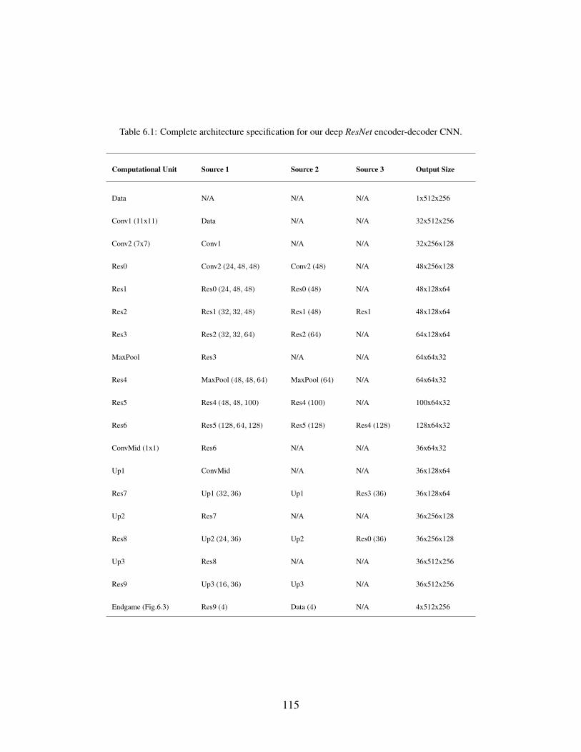
Table 6.1: Complete architecture specification for our deep ResNet encoder-decoder CNN.

Computational Unit Source 1 Source 2 Source 3 Output Size

Data N/A N/A N/A 1x512x256

Conv1 (11x11) Data N/A N/A 32x512x256

Conv2 (7x7) Conv1 N/A N/A 32x256x128

Res0 Conv2 (24, 48, 48) Conv2 (48) N/A 48x256x128

Res1 Res0 (24, 48, 48) Res0 (48) N/A 48x128x64

Res2 Res1 (32, 32, 48) Res1 (48) Res1 48x128x64

Res3 Res2 (32, 32, 64) Res2 (64) N/A 64x128x64

MaxPool Res3 N/A N/A 64x64x32

Res4 MaxPool (48, 48, 64) MaxPool (64) N/A 64x64x32

Res5 Res4 (48, 48, 100) Res4 (100) N/A 100x64x32

Res6 Res5 (128, 64, 128) Res5 (128) Res4 (128) 128x64x32

ConvMid (1x1) Res6 N/A N/A 36x64x32

Up1 ConvMid N/A N/A 36x128x64

Res7 Up1 (32, 36) Up1 Res3 (36) 36x128x64

Up2 Res7 N/A N/A 36x256x128

Res8 Up2 (24, 36) Up2 Res0 (36) 36x256x128

Up3 Res8 N/A N/A 36x512x256

Res9 Up3 (16, 36) Up3 N/A 36x512x256

Endgame (Fig.6.3) Res9 (4) Data (4) N/A 4x512x256

115

Post-Processing.

We utilized multiple post-processing algorithms to improve upon the CNN output before con-

structing the final output. Central to the post-processing is the graph-cut algorithm [110–112]. We

utilized a MATLAB wrapper [113] of the Boykov-Kolmogorov graph cut implementation. Prior

to graph cut, we zeroed out IRF probabilities on edge pixels (based on Difference-of-Gaussians

(DoG)) and modestly decreased SRF and PED probabilities on bright pixels in continuous fashion,

according to equation 6.1. Specifically, we used T1(µ(I), σ(I)) = µ(I)+σ(I) and T2(µ(I), σ(I)) =

µ(I) + 3σ(I), with λ = 0 for SRF and 0.95 for PED.

P (x, y) =

P ′(x, y), I(x, y) ≤ T1(µ(I), σ(I))

P ′(x, y) max(λ, T2(µ(I),σ(I))−I(x,y)T2(µ(I),σ(I))−T1(µ(I),σ(I))), otherwise.

(6.1)

These operations define the prior class probabilities used by the graph-cut algorithm. The data cost

was set to the negative logarithm of the prior. The base smoothness cost (penalty for neighbor-

ing pixels having different labels) was set to 5 for IRF/non-fluid, 10 for all other different label

combinations, and 0 for adjacent pixels having the same label. This cost was then multiplied by

a spatially varying smoothness cost, set from the result of applying a DoG filter to the image. In

particular, the full smoothness cost is specified in equation 6.2, with S ′ the base smoothness cost

and g(I) equal to the result of the DoG operation.

S = S ′ exp(−5g(I)/max(g(I))). (6.2)

After graph cut, we invoked two additional post-processing steps. The first enforces the rule that

116

PED cannot occur above IRF or SRF. The approach here is very straightforward. For each vertical

line within which PED and either IRF or SRF were contained, the topmost PED pixel was found,

and then the topmost IRF or SRF pixel beneath the topmost PED pixel was found. Counts were

obtained for the number of pixels belonging to PED and the number of pixels belonging to the other

identified fluid beneath the first PED occurrence. The larger count “wins," meaning that all pixels

of the "losing" fluid have their labels replaced by the "winning" fluid. The final post-processing

step here was some PED connected component analysis, which simply removed PED connected

components that didn’t meet criteria for a minimum slope change across the top (the logic being

that the top of a PED occurrence is never a straight line).

These steps resulted in each slice of the OCT volume having been fully processed in its own right,

but without leveraging any 3D information; obviously, there should be reasonable agreement be-

tween adjacent slices of the same OCT volume. To leverage this, we built the result volumes and

then ran graph cut on all of the yz-plane slices. The result volumes constructed at this stage were

"uncropped" back to the standard size of 512x496, but were not resized to the original image sizes

until after running graph cut on the yz-plane slices (see section 6). For this graph cut, the smooth-

ness cost was set the same way as described earlier for the xy-plane results, except a different

parameterization for the DoG filter was used. The data cost at each pixel was zero for the current

label at that pixel and a positive constant for the other three classes.

Results

We have tested our method on two different data sets that were manually annotated by experts,

using two-fold cross-validation in each case. The data sets are quite different from each other.

One contains a fairly large number of patients with only one OCT scan per patient, while the other

contains several OCT scans of a handful of patients measured over a lengthy period of time during

117

which the patients were receiving treatment.

Experiments on RETOUCH Data Set

We evaluated our method on the RETOUCH data set by computing dice index and absolute volume

difference (AVD), alongside a qualitative evaluation through visual inspection. The results were

generated using two-fold cross-validation, with the two subsets having roughly equal amounts of

each fluid type and roughly an equal number of scans from each device.

Qualitatively, our method was observed to be capable of obtaining very good results, as visually

verified by the participating ophthalmologist, but there were also some challenging cases. Some

examples are shown in Figures 6.4 and 6.5a, respectively. However, upon inspection of the entire

provided dataset, we unfortunately felt that the provided reference standard was at best less than

pristine, and at worst remarkably inconsistent, especially for IRF. Some examples are shown in

Figure 6.5b). For both of these figures, the output of our method is shown on top and the reference

standard is shown on bottom (Red = IRF, green = SRF, blue = PED).

Figure 6.4: Examples on which our method performed extremely well.

118

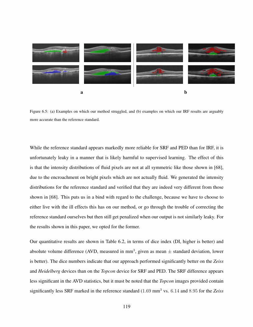
a b

Figure 6.5: (a) Examples on which our method struggled, and (b) examples on which our IRF results are arguably

more accurate than the reference standard.

While the reference standard appears markedly more reliable for SRF and PED than for IRF, it is

unfortunately leaky in a manner that is likely harmful to supervised learning. The effect of this

is that the intensity distributions of fluid pixels are not at all symmetric like those shown in [68],

due to the encroachment on bright pixels which are not actually fluid. We generated the intensity

distributions for the reference standard and verified that they are indeed very different from those

shown in [68]. This puts us in a bind with regard to the challenge, because we have to choose to

either live with the ill effects this has on our method, or go through the trouble of correcting the

reference standard ourselves but then still get penalized when our output is not similarly leaky. For

the results shown in this paper, we opted for the former.

Our quantitative results are shown in Table 6.2, in terms of dice index (DI, higher is better) and

absolute volume difference (AVD, measured in mm3, given as mean ± standard deviation, lower

is better). The dice numbers indicate that our approach performed significantly better on the Zeiss

and Heidelberg devices than on the Topcon device for SRF and PED. The SRF difference appears

less significant in the AVD statistics, but it must be noted that the Topcon images provided contain

significantly less SRF marked in the reference standard (1.69 mm3 vs. 6.14 and 8.95 for the Zeiss

119

and Heidelberg data sets respectively).

Table 6.2: Quantitative results on RETOUCH data set.

Measure Zeiss Heidelberg Topcon All Devices

DI (IRF) 0.537 0.478 0.547 0.522

DI (SRF) 0.671 0.781 0.483 0.682

DI (PED) 0.699 0.610 0.459 0.612

AVD (IRF) 0.248±0.429 0.296±0.379 0.115±0.139 0.285±0.481

AVD (SRF) 0.089±0.154 0.103±0.158 0.073±0.152 0.115±0.207

AVD (PED) 0.174±0.336 0.086±0.155 0.222±0.470 0.156±0.287

As part of the RETOUCH grand challenge at MICCAI 2017, we also trained on the entire data set

and then generated results on the official RETOUCH test set, for which labels were not provided.

Our method obtained second place in the detection challenge, which was graded by area under

the receiver operating characteristic (ROC) curves for each fluid type. The challenge organizers

generated the curves based on CSV-formatted output provided by each team containing probability

measures for the presence of each fluid type in each scan. Our official ROC curve is shown in

Figure 6.6.

120

Figure 6.6: Fluid detection ROC curves obtained by our method in the RETOUCH challenge.

Experiments on Alternate Data Set

As mentioned earlier, the alternate data set contains a small number of patients, but multiple scans

per patient. Because the patients were undergoing treatment, different scans of the same patient

did tend to look fairly different. For this reason, the split for two-fold cross validation was obtained

by, for each patient p, putting the first kp scans in one set and the remaining scans in the other set.

The logic here is that while there might conceivably be a high degree of similarity between scan

k and scan k + 1 of the same patient, the similarity should degrade as the scans get further and

further apart in time.

121

Some of these patients had particularly swollen retinas, to the effect that the vertical crop size

of 256 that was used on the RETOUCH data set was frequently not large enough to capture all

of the fluid. The crop size was therefore enlarged to 512 (resulting in square images), which

resulted in capturing more than 99% of the fluid pixels. This had the further consequence of

additional memory consumption, as the prior configuration already resulted in maxing out the

memory capacity of the GPU. To resolve this, the stride was changed to 2 in the Conv1 layer, and

an additional upsampling layer was inserted in between Up3 and Res9.

Using the central three quarters of each OCT volume, two-fold cross validation was performed.

The data augmentation was the same as that used on the RETOUCH data, except fewer rotations

were used (−6◦ to +6◦ in increments of 3◦) since there was a larger total amount of data available.

This data set actually contained distinct labels for CNV vs. PED. The data set contained a total

of 67 scans from 5 patients, with CNV present in all patients, SRF present in all but one patient,

and cystoid edema (or intraretinal fluid, IRF) and PED were only present in two patients each. In

private discussions with an ophthalmologist, it was suggested that distinguishing between CNV

and PED may not be all that useful and it might even be poorly defined. This was subsequently

borne out in initial experiments, which showed extremely poor performance on PED as compared

with the other pathologies (dice scores below 0.2). For this reason, the PED and CNV were merged

into a single category, which effectively changed the labeling to the same conventions used in the

RETOUCH data set. The results from training the CNN for 2 epochs at a learning rate of 5× 10−5

and 1 epoch with the learning rate reduced by a factor of 10 are shown in Table 6.3, once again in

terms of dice index (DI, higher is better) and absolute volume difference (AVD, measured in mm3,

given as mean ± standard deviation, lower is better).

122

Table 6.3: Quantitative results on alternate data set.

Measure IRF SRF CNV/PED

DI 0.389 0.677 0.662

AVD 0.076±0.121 0.182±0.259 0.626±0.513

The dice indices are very consistent with what was obtained on the RETOUCH data, even though

post-processing was not performed. This indicates that the pre-processing and data augmenta-

tion frameworks as well as the CNN architecture are indeed very well suited to pathological fluid

detection and classification.

The AVD is significantly higher for PED/CNV than for the other fluids. The main factor responsi-

ble for that is simply that this data set contains a lot more PED/CNV than the other fluid types (it is

present in every scan). Regardless, the high standard deviation still points to the fact that there are

some images on which our method does extremely well and some on which it does poorly. There

are multiple things going on here that could explain this phenomenon. One possible factor is mul-

tiple different biological phenomena sharing the same label ("pure" PED and CNV), combined

with the limited training set size. Additionally, it is conceivable that alternate CNN configurations

would reduce the spreads. On the one hand, this possibility is difficult to consider due to the fact

that multiple configurations were tried (albeit on the RETOUCH data set) before settling on the

described design. On the other hand, the space of possible CNN configurations is limitless, so

this is impossible to rule out. However, the weighted loss function could definitely be a factor,

as the CNN wound up significantly more prone to false positives than negatives despite setting

the weights in accordance with label statistics. Finally, including retina layer segmentation as a

123

pre-processing step would probably reduce all of the spreads, since this significantly restricts the

space of allowed pixel locations for each label type (which would also feed into the configuration

of the weighted loss function).

Conclusion

We presented a deep learning based method for simultaneously and automatically detecting and

segmenting intraretinal fluid, subretinal fluid, and pigment epithelial detachment in OCT images

of the human retina. We also presented a novel data augmentation method for these images called

myopic warping. We obtained decent results on two different data sets. Remarkably, our method

did not involve any kind of precise retinal segmentation, and it stands to reason that our method

could potentially be improved by adding one to the pre-processing or post-processing steps. We

believe that in time, deep learning will prove to be a necessary component to obtaining state-of-

the-art results on the automatic fluid segmentation problem.

124

CHAPTER 7: CONCLUSION

Ophthalmic computer vision is an intriguing subset of medical computer vision that utilizes a wide

array of imaging modalities to analyze different parts of the human eye. Applications include

automatic segmentation and registration in the anterior segment for various laser surgeries, as well

as various detection, classification, and measurement tasks associated with pathologies. We have

presented multiple significant contributions to this field.

Chapter 3 presented a solution to the problem of accounting for cyclotorsion in refractive laser eye

surgery. Cyclotorsion is a significant rotation of the eye within its socket that occurs when a per-

son transitions from sitting or standing to lying down. The solution presented is an automatic iris

registration algorithm. By necessity, the algorithm accomplishes the registration under both rigid

and non-rigid deformations, with pupil dilation being the primary cause of non-rigid deforma-

tions. The method differs greatly from previous work on iris registration in that it does not rely on

tracking feature correspondences, but rather defines and optimizes an inner product between two

unwrapped iris images. Embedded within the inner product is a radial shear function to account

for non-rigid deformations while also making the registration more robust to segmentation errors.

Manual validation of the algorithm was performed using humans trained to identify point corre-

spondences between two images of the same iris, and this showed that the algorithm is extremely

accurate. Indeed, the algorithm matched the average cyclotorsion measured by the humans with

greater consistency than any individual human. The algorithm contains a robust built-in confidence

metric, which can be conservatively thresholded based on statistics to guarantee performance lev-

els in terms of false positive rate (rejecting a correct registration due to poor confidence) and false

negative rate (accepting an incorrect registration). Importantly, the statistical analysis presented

for this task does not require any actual incorrect registrations to be present in the data sample in

order to compute the desired conservative estimates. This is because the analysis leverages the fact

125

that the algorithm outputs the global maximum of the inner product defined for the registration,

specifically by comparing the maximum corresponding to the correct cyclotorsion angle with other

local maxima for each eye in the data set. In addition to the method and analysis, Chapter 3 also

explored the intricate relationship between iris registration and iris recognition. In particular, it was

argued that any method performing well on one task should be able to be recast as a method that

also performs well on the other task. Based on this insight, the iris registration method developed

in the chapter combines elements from prior work on both problems. This work is published in

IEEE Transactions on Biomedical Engineering.

Chapter 4 presented an extension to the iris registration algorithm from Chapter 3 in which the

alignment of unwrapping centers is simultaneously optimized while identifying the angle of cy-

clotorsion. We showed that this improves the success rate of cyclotorsion identification while

also providing a secondary output (the optimized unwrapping center) which may be of anatomi-

cal interest in certain circumstances. In particular, the optimized unwrapping center in the second

image tracks very closely with the pupil center in the first image, providing a reasonably accurate

method for identifying the photopic pupil center in a dilated eye without requiring the patient to

fixate. Interestingly, this extension was implemented using backpropagation, despite the fact that

the algorithm does not use any machine learning.

Chapter 5 explored a novel framework for improving RANSAC-based segmentation algorithms

using convolutional neural networks (CNN). This is relevant to ophthalmic computer vision be-

cause many surfaces of the eye have specific shapes with low numbers of degrees of freedom

(i.e. circles), which makes RANSAC a highly effective segmentation technique for these surfaces.

As an example, RANSAC was used for pupil segmentation in the iris registration algorithm of

Chapter 3. The method presented in Chapter 5 for improving such algorithms is to convert the

pre-RANSAC feature extraction steps into CNN layers and fine-tune the resulting CNN with a

novel RANSAC-based loss function. In the case of pupil segmentation, this amounts to creating a

126

CNN that detects pupil edges. Nearly all the steps of classical edge detectors can be represented

exactly or near-exactly by differentiable computation layers, including, of course, convolution

layers. Such convolution layers may be zero-padded to provide extra learning parameters while

preserving initial performance, and custom layers can be utilized for calculations such as L2 norm.

The method was tested on a large iris recognition data set for which annotated ground truth data

were readily available. On this data, segmentation improvement through CNN fine-tuning was

successfully demonstrated. This work can therefore be summarized as a highly novel application

of state-of-the-art machine learning methods in a way that is maximally complementary to solid

non-learning (or classical) methods. Importantly, the main ideas behind the methodology are not

limited to segmentation by any stretch; there are a multitude of methods for solving 3D computer

vision problems that utilize RANSAC following a keypoint detection step, and the methodology

of Chapter 5 could analogously be applied to these approaches by using a CNN as the keypoint

detector. This work was presented in full at CVPR 2017.

Chapter 6 presented a more wholesale application of state-of-the-art deep learning methods through

constructing a CNN to simultaneously detect and segment three different types of retina fluid: in-

traretinal fluid, subretinal fluid, and pigment epithelial detachment. The CNN operates on OCT

imagery, which is the state-of-the-art method used by ophthalmologists to assess retina health

in detail. The CNN embodies ResNet and encoder-decoder strategies. The principal benefit of

ResNet is the ability to make the CNN extremely deep, while the main benefit of encoder-decoder

is the ability to generate output of the same size as the input. A novel data augmentation technique

dubbed myopic warping was utilized to greatly increase the size of the data set. This technique

produced multiple warped versions of each image, each differing from the original by appearing

as though it came from a more myopic eye (in practical terms, an eye with a curvier retina). The

CNN output was post-processed with graph cut and some other knowledge guided morphological

operations. This work was done as part of the 2017 RETOUCH grand challenge, which graded

127

participants on both detection and segmentation. The method achieved second place in detection,

which means the CNN did extremely well at ranking different OCT images by the amount of each

fluid volume present. The method was also shown to obtain similar performance (in terms of dice

index and absolute volume difference) on a separate data set.

One of the larger goals of our work was to leverage insights from both classical computer vision

and modern deep learning to design algorithms that leverage the best of both worlds. To that end,

the works described in this dissertation slotted in all throughout the spectrum between classical

computer vision and modern machine learning approaches. The especially interesting cases are

those near the middle of the spectrum, which are the use of backpropagation in Chapter 4 and

the RANSAC-guided CNN in Chapter 5. One might also be tempted to place the novel myopic

warping data augmentation technique from Chapter 6 in this category, since that technique is so

heavily guided by specific knowledge of the problem domain in which it is applied. Undoubtedly,

this boundary between deep learning and classical methods is one of the most interesting sub-fields

of computer vision in our day, and we look forward to continued progress on this front as time goes

on.

128

APPENDIX : COPYRIGHT INFORMATION

129

IEEE COPYRIGHT FORM

To ensure uniformity of treatment among all contributors, other forms may not be substituted for this form, nor may any wording

of the form be changed. This form is intended for original material submitted to the IEEE and must accompany any such material

in order to be published by the IEEE. Please read the form carefully and keep a copy for your files.

Computing Cyclotorsion in Refractive Cataract Surgery

Morley, Dustin; Foroosh, Hassan

Transactions on Biomedical Engineering

COPYRIGHT TRANSFERThe undersigned hereby assigns to The Institute of Electrical and Electronics Engineers, Incorporated (the "IEEE") all rights

under copyright that may exist in and to: (a) the Work, including any revised or expanded derivative works submitted to the IEEE

by the undersigned based on the Work; and (b) any associated written or multimedia components or other enhancements

accompanying the Work.

GENERAL TERMS1. The undersigned represents that he/she has the power and authority to make and execute this form.

2. The undersigned agrees to indemnify and hold harmless the IEEE from any damage or expense that may arise in the event of

a breach of any of the warranties set forth above.

3. The undersigned agrees that publication with IEEE is subject to the policies and procedures of the IEEE PSPB Operations

Manual.

4. In the event the above work is not accepted and published by the IEEE or is withdrawn by the author(s) before acceptance by

the IEEE, the foregoing grant of rights shall become null and void and all materials embodying the Work submitted to the IEEE

will be destroyed.

5. For jointly authored Works, all joint authors should sign, or one of the authors should sign as authorized agent for the others.

6. The author hereby warrants that the Work and Presentation (collectively, the "Materials") are original and that he/she is the

author of the Materials. To the extent the Materials incorporate text passages, figures, data or other material from the works of

others, the author has obtained any necessary permissions. Where necessary, the author has obtained all third party permissions

and consents to grant the license above and has provided copies of such permissions and consents to IEEE

BY TYPING IN YOUR FULL NAME BELOW AND CLICKING THE SUBMIT BUTTON, YOU CERTIFY THAT SUCH ACTION

CONSTITUTES YOUR ELECTRONIC SIGNATURE TO THIS FORM IN ACCORDANCE WITH UNITED STATES LAW, WHICH

AUTHORIZES ELECTRONIC SIGNATURE BY AUTHENTICATED REQUEST FROM A USER OVER THE INTERNET AS A

VALID SUBSTITUTE FOR A WRITTEN SIGNATURE.

Information for Authors

AUTHOR RESPONSIBILITIES

The IEEE distributes its technical publications throughout the world and wants to ensure that the material submitted to its

publications is properly available to the readership of those publications. Authors must ensure that their Work meets the

requirements as stated in section 8.2.1 of the IEEE PSPB Operations Manual, including provisions covering originality,

       Dustin Morley              21-12-2015

       Signature

             Date (dd-mm-yyyy)

130

-

-

-

-

-

-

-

authorship, author responsibilities and author misconduct. More information on IEEE's publishing policies may be found at

http://www.ieee.org/publications_standards/publications/rights/authorrightsresponsibilities.html Authors are advised especially of

IEEE PSPB Operations Manual section 8.2.1.B12: "It is the responsibility of the authors, not the IEEE, to determine whether

disclosure of their material requires the prior consent of other parties and, if so, to obtain it." Authors are also advised of IEEE

PSPB Operations Manual section 8.1.1B: "Statements and opinions given in work published by the IEEE are the expression of

the authors."

RETAINED RIGHTS/TERMS AND CONDITIONS

Authors/employers retain all proprietary rights in any process, procedure, or article of manufacture described in the Work.

Authors/employers may reproduce or authorize others to reproduce the Work, material extracted verbatim from the Work, or

derivative works for the author's personal use or for company use, provided that the source and the IEEE copyright notice are

indicated, the copies are not used in any way that implies IEEE endorsement of a product or service of any employer, and the

copies themselves are not offered for sale.

Although authors are permitted to re-use all or portions of the Work in other works, this does not include granting third-party

requests for reprinting, republishing, or other types of re-use.The IEEE Intellectual Property Rights office must handle all such

third-party requests.

Authors whose work was performed under a grant from a government funding agency are free to fulfill any deposit mandates

from that funding agency.

AUTHOR ONLINE USEPersonal Servers. Authors and/or their employers shall have the right to post the accepted version of IEEE-copyrighted

articles on their own personal servers or the servers of their institutions or employers without permission from IEEE, provided

that the posted version includes a prominently displayed IEEE copyright notice and, when published, a full citation to the

original IEEE publication, including a link to the article abstract in IEEE Xplore. Authors shall not post the final, published

versions of their papers.

Classroom or Internal Training Use. An author is expressly permitted to post any portion of the accepted version of his/her

own IEEE-copyrighted articles on the author's personal web site or the servers of the author's institution or company in

connection with the author's teaching, training, or work responsibilities, provided that the appropriate copyright, credit, and

reuse notices appear prominently with the posted material. Examples of permitted uses are lecture materials, course packs, e-

reserves, conference presentations, or in-house training courses.

Electronic Preprints. Before submitting an article to an IEEE publication, authors frequently post their manuscripts to their

own web site, their employer's site, or to another server that invites constructive comment from colleagues. Upon submission

of an article to IEEE, an author is required to transfer copyright in the article to IEEE, and the author must update any

previously posted version of the article with a prominently displayed IEEE copyright notice. Upon publication of an article by

the IEEE, the author must replace any previously posted electronic versions of the article with either (1) the full citation to the

IEEE work with a Digital Object Identifier (DOI) or link to the article abstract in IEEE Xplore, or (2) the accepted version only

(not the IEEE-published version), including the IEEE copyright notice and full citation, with a link to the final, published article

in IEEE Xplore.

Questions about the submission of the form or manuscript must be sent to the publication's editor.

Please direct all questions about IEEE copyright policy to:

IEEE Intellectual Property Rights Office, copyrights@ieee.org, +1-732-562-3966

131

1.

2.

3.

4.

5.

6.

1.

2.

IEEE COPYRIGHT AND CONSENT FORM

To ensure uniformity of treatment among all contributors, other forms may not be substituted for this form, nor may any wording

of the form be changed. This form is intended for original material submitted to the IEEE and must accompany any such material

in order to be published by the IEEE. Please read the form carefully and keep a copy for your files.

Improving RANSAC-Based Segmentation Through CNN Encapsulation

Dustin Morley and Hassan Foroosh

2017 IEEE Conference on Computer Vision and Pattern Recognition (CVPR)

COPYRIGHT TRANSFERThe undersigned hereby assigns to The Institute of Electrical and Electronics Engineers, Incorporated (the "IEEE") all rights

under copyright that may exist in and to: (a) the Work, including any revised or expanded derivative works submitted to the IEEE

by the undersigned based on the Work; and (b) any associated written or multimedia components or other enhancements

accompanying the Work.

GENERAL TERMS

The undersigned represents that he/she has the power and authority to make and execute this form.

The undersigned agrees to indemnify and hold harmless the IEEE from any damage or expense that may arise in the

event of a breach of any of the warranties set forth above.

The undersigned agrees that publication with IEEE is subject to the policies and procedures of the IEEE PSPB

Operations Manual.

In the event the above work is not accepted and published by the IEEE or is withdrawn by the author(s) before

acceptance by the IEEE, the foregoing copyright transfer shall be null and void. In this case, IEEE will retain a copy of

the manuscript for internal administrative/record-keeping purposes.

For jointly authored Works, all joint authors should sign, or one of the authors should sign as authorized agent for the

others.

The author hereby warrants that the Work and Presentation (collectively, the "Materials") are original and that he/she is

the author of the Materials. To the extent the Materials incorporate text passages, figures, data or other material from the

works of others, the author has obtained any necessary permissions. Where necessary, the author has obtained all third

party permissions and consents to grant the license above and has provided copies of such permissions and consents

to IEEE

You have indicated that you DO wish to have video/audio recordings made of your conference presentation under terms

and conditions set forth in "Consent and Release."

CONSENT AND RELEASE

ln the event the author makes a presentation based upon the Work at a conference hosted or sponsored in whole or in

part by the IEEE, the author, in consideration for his/her participation in the conference, hereby grants the IEEE the

unlimited, worldwide, irrevocable permission to use, distribute, publish, license, exhibit, record, digitize, broadcast,

reproduce and archive, in any format or medium, whether now known or hereafter developed: (a) his/her presentation

and comments at the conference; (b) any written materials or multimedia files used in connection with his/her

presentation; and (c) any recorded interviews of him/her (collectively, the "Presentation"). The permission granted

includes the transcription and reproduction of the Presentation for inclusion in products sold or distributed by IEEE and

live or recorded broadcast of the Presentation during or after the conference.

In connection with the permission granted in Section 1, the author hereby grants IEEE the unlimited, worldwide,

irrevocable right to use his/her name, picture, likeness, voice and biographical information as part of the advertisement,

distribution and sale of products incorporating the Work or Presentation, and releases IEEE from any claim based on

right of privacy or publicity.

132

-

-

-

-

-

-

-

BY TYPING IN YOUR FULL NAME BELOW AND CLICKING THE SUBMIT BUTTON, YOU CERTIFY THAT SUCH ACTION

CONSTITUTES YOUR ELECTRONIC SIGNATURE TO THIS FORM IN ACCORDANCE WITH UNITED STATES LAW, WHICH

AUTHORIZES ELECTRONIC SIGNATURE BY AUTHENTICATED REQUEST FROM A USER OVER THE INTERNET AS A

VALID SUBSTITUTE FOR A WRITTEN SIGNATURE.

Information for Authors

AUTHOR RESPONSIBILITIES

The IEEE distributes its technical publications throughout the world and wants to ensure that the material submitted to its

publications is properly available to the readership of those publications. Authors must ensure that their Work meets the

requirements as stated in section 8.2.1 of the IEEE PSPB Operations Manual, including provisions covering originality,

authorship, author responsibilities and author misconduct. More information on IEEE’s publishing policies may be found at

http://www.ieee.org/publications_standards/publications/rights/authorrightsresponsibilities.html Authors are advised especially of

IEEE PSPB Operations Manual section 8.2.1.B12: "It is the responsibility of the authors, not the IEEE, to determine whether

disclosure of their material requires the prior consent of other parties and, if so, to obtain it." Authors are also advised of IEEE

PSPB Operations Manual section 8.1.1B: "Statements and opinions given in work published by the IEEE are the expression of

the authors."

RETAINED RIGHTS/TERMS AND CONDITIONSAuthors/employers retain all proprietary rights in any process, procedure, or article of manufacture described in the Work.

Authors/employers may reproduce or authorize others to reproduce the Work, material extracted verbatim from the Work, or

derivative works for the author's personal use or for company use, provided that the source and the IEEE copyright notice are

indicated, the copies are not used in any way that implies IEEE endorsement of a product or service of any employer, and the

copies themselves are not offered for sale.

Although authors are permitted to re-use all or portions of the Work in other works, this does not include granting third-party

requests for reprinting, republishing, or other types of re-use.The IEEE Intellectual Property Rights office must handle all such

third-party requests.

Authors whose work was performed under a grant from a government funding agency are free to fulfill any deposit mandates

from that funding agency.

AUTHOR ONLINE USEPersonal Servers. Authors and/or their employers shall have the right to post the accepted version of IEEE-copyrighted

articles on their own personal servers or the servers of their institutions or employers without permission from IEEE, provided

that the posted version includes a prominently displayed IEEE copyright notice and, when published, a full citation to the

original IEEE publication, including a link to the article abstract in IEEE Xplore. Authors shall not post the final, published

versions of their papers.

Classroom or Internal Training Use. An author is expressly permitted to post any portion of the accepted version of his/her

own IEEE-copyrighted articles on the author's personal web site or the servers of the author's institution or company in

connection with the author's teaching, training, or work responsibilities, provided that the appropriate copyright, credit, and

reuse notices appear prominently with the posted material. Examples of permitted uses are lecture materials, course packs, e-

reserves, conference presentations, or in-house training courses.

Electronic Preprints. Before submitting an article to an IEEE publication, authors frequently post their manuscripts to their

own web site, their employer's site, or to another server that invites constructive comment from colleagues. Upon submission

of an article to IEEE, an author is required to transfer copyright in the article to IEEE, and the author must update any

previously posted version of the article with a prominently displayed IEEE copyright notice. Upon publication of an article by

the IEEE, the author must replace any previously posted electronic versions of the article with either (1) the full citation to the

       Dustin Morley              07-04-2017

       Signature

             Date (dd-mm-yyyy)

133

IEEE work with a Digital Object Identifier (DOI) or link to the article abstract in IEEE Xplore, or (2) the accepted version only

(not the IEEE-published version), including the IEEE copyright notice and full citation, with a link to the final, published article

in IEEE Xplore.

Questions about the submission of the form or manuscript must be sent to the publication's editor.

Please direct all questions about IEEE copyright policy to:

IEEE Intellectual Property Rights Office, copyrights@ieee.org, +1-732-562-3966

134

LIST OF REFERENCES

[1] D. Morley and H. Foroosh, “Computing cyclotorsion in refractive cataract surgery,” IEEE

Transactions on Biomedical Engineering, vol. 63, no. 10, pp. 2155–2168, 2016.

[2] M. D. Zeiler and R. Fergus, “Visualizing and understanding convolutional networks,” in

European Conference on Computer Vision. Springer, 2014, pp. 818–833.

[3] M. A. Fischler and R. C. Bolles, “Random sample consensus: a paradigm for model fitting

with applications to image analysis and automated cartography,” Communications of the

ACM, vol. 24, no. 6, pp. 381–395, 1981.

[4] K. Tanaka and E. Kondo, “Incremental ransac for online relocation in large dynamic en-

vironments,” in 2006 IEEE International Conference on Robotics and Automation (ICRA).

IEEE, 2006, pp. 68–75.

[5] S.-W. Yang, C.-C. Wang, and C.-H. Chang, “Ransac matching: Simultaneous registration

and segmentation,” in Robotics and Automation (ICRA), 2010 IEEE International Confer-

ence on. IEEE, 2010, pp. 1905–1912.

[6] M. Waine, C. Rossa, R. Sloboda, N. Usmani, and M. Tavakoli, “3d shape visualization of

curved needles in tissue from 2d ultrasound images using ransac,” in 2015 IEEE Interna-

tional Conference on Robotics and Automation (ICRA). IEEE, 2015, pp. 4723–4728.

[7] C. Papalazarou, P. M. Rongen, and P. H. de With, “Multiple model estimation for the de-

tection of curvilinear segments in medical x-ray images using sparse-plus-dense-ransac,”

in Pattern Recognition (ICPR), 2010 20th International Conference on. IEEE, 2010, pp.

2484–2487.

135

[8] S. K. Kim, H.-J. Kong, J.-M. Seo, B. J. Cho, K. H. Park, J. M. Hwang, D.-M. Kim,

H. Chung, and H. C. Kim, “Segmentation of optic nerve head using warping and ransac,”

in 2007 29th Annual International Conference of the IEEE Engineering in Medicine and

Biology Society. IEEE, 2007, pp. 900–903.

[9] R. Rocha, A. Campilho, J. Silva, E. Azevedo, and R. Santos, “Segmentation of ultrasound

images of the carotid using ransac and cubic splines,” Computer methods and programs in

biomedicine, vol. 101, no. 1, pp. 94–106, 2011.

[10] P. H. Torr and A. Zisserman, “Mlesac: A new robust estimator with application to estimating

image geometry,” Computer Vision and Image Understanding, vol. 78, no. 1, pp. 138–156,

2000.

[11] P. H. Torr and D. W. Murray, “The development and comparison of robust methods for

estimating the fundamental matrix,” International journal of computer vision, vol. 24, no. 3,

pp. 271–300, 1997.

[12] V. Dvornychenko, “Bounds on (deterministic) correlation functions with application to reg-

istration,” IEEE Transactions on Pattern Analysis and Machine Intelligence, no. 2, pp. 206–

213, 1983.

[13] R. J. Althof et al., “A rapid and automatic image registration algorithm with subpixel accu-

racy,” Medical Imaging, IEEE Transactions on, vol. 16, no. 3, pp. 308–316, 1997.

[14] H. Foroosh et al., “Extension of phase correlation to subpixel registration,” Image Process-

ing, IEEE Transactions on, vol. 11, no. 3, pp. 188–200, 2002.

[15] M. Balci and H. Foroosh, “Subpixel estimation of shifts directly in the fourier domain,”

Image Processing, IEEE Transactions on, vol. 15, no. 7, pp. 1965–1972, 2006.

136

[16] W. S. Hoge, “A subspace identification extension to the phase correlation method [mri ap-

plication],” Medical Imaging, IEEE Transactions on, vol. 22, no. 2, pp. 277–280, 2003.

[17] W. S. Hoge and C.-F. Westin, “Identification of translational displacements between n-

dimensional data sets using the high-order svd and phase correlation,” Image Processing,

IEEE Transactions on, vol. 14, no. 7, pp. 884–889, 2005.

[18] U.-V. Koc and K. R. Liu, “Interpolation-free subpixel motion estimation techniques in dct

domain,” Circuits and Systems for Video Technology, IEEE Transactions on, vol. 8, no. 4,

pp. 460–487, 1998.

[19] C. D. Hummel, V. F. Diakonis, N. R. Desai, A. Arana, and R. J. Weinstock, “Cyclorota-

tion during femtosecond laser–assisted cataract surgery measured using iris registration,”

Journal of Cataract & Refractive Surgery, vol. 43, no. 7, pp. 952–955, 2017.

[20] A. U. Swami et al., “Rotational malposition during laser in situ keratomileusis,” American

journal of ophthalmology, vol. 133, no. 4, pp. 561–562, 2002.

[21] G. Krieglstein, “Andrew coombes, david gartry (eds): Cataract surgery,” Graefe’s Archive

for Clinical and Experimental Ophthalmology, vol. 241, no. 12, pp. 1055–1055, 2003.

[22] N. Visser et al., “Accuracy of toric intraocular lens implantation in cataract and refractive

surgery,” Journal of Cataract & Refractive Surgery, vol. 37, no. 8, pp. 1394–1402, 2011.

[23] D. A. Chernyak, “Iris-based cyclotorsional image alignment method for wavefront regis-

tration,” Biomedical Engineering, IEEE Transactions on, vol. 52, no. 12, pp. 2032–2040,

2005.

[24] J. G. Daugman, “High confidence visual recognition of persons by a test of statistical in-

dependence,” Pattern Analysis and Machine Intelligence, IEEE Transactions on, vol. 15,

no. 11, pp. 1148–1161, 1993.

137

[25] ——, “Biometric personal identification system based on iris analysis,” Mar. 1 1994, uS

Patent 5,291,560.

[26] K. W. Bowyer et al., “Image understanding for iris biometrics: A survey,” Computer vision

and image understanding, vol. 110, no. 2, pp. 281–307, 2008.

[27] R. P. Wildes, “Iris recognition: an emerging biometric technology,” Proceedings of the

IEEE, vol. 85, no. 9, pp. 1348–1363, 1997.

[28] X. Liu et al., “Experiments with an improved iris segmentation algorithm,” in Automatic

Identification Advanced Technologies, 2005. Fourth IEEE Workshop on. IEEE, 2005, pp.

118–123.

[29] Z. He, T. Tan, Z. Sun, and X. Qiu, “Toward accurate and fast iris segmentation for iris

biometrics,” IEEE transactions on pattern analysis and machine intelligence, vol. 31, no. 9,

pp. 1670–1684, 2009.

[30] S. Shah and A. Ross, “Iris segmentation using geodesic active contours,” Information Foren-

sics and Security, IEEE Transactions on, vol. 4, no. 4, pp. 824–836, 2009.

[31] J. Daugman, “New methods in iris recognition,” Systems, Man, and Cybernetics, Part B:

Cybernetics, IEEE Transactions on, vol. 37, no. 5, pp. 1167–1175, 2007.

[32] L. Ma, Y. Wang, and T. Tan, “Iris recognition using circular symmetric filters,” in Pattern

Recognition, 2002. Proceedings. 16th International Conference on, vol. 2. IEEE, 2002,

pp. 414–417.

[33] S. Lim, K. Lee, O. Byeon, and T. Kim, “Efficient iris recognition through improvement of

feature vector and classifier,” ETRI journal, vol. 23, no. 2, pp. 61–70, 2001.

[34] D. M. Monro, S. Rakshit, and D. Zhang, “Dct-based iris recognition,” IEEE Transactions

on Pattern Analysis and Machine Intelligence, vol. 29, no. 4, pp. 586–595, 2007.

138

[35] F. Shen and P. J. Flynn, “Iris matching by crypts and anti-crypts,” in Homeland Security

(HST), 2012 IEEE Conference on Technologies for. IEEE, 2012, pp. 208–213.

[36] J. Chen, F. Shen, D. Z. Chen, and P. J. Flynn, “Iris recognition based on human-interpretable

features,” IEEE Transactions on Information Forensics and Security, vol. 11, no. 7, pp.

1476–1485, 2016.

[37] D. A. Robinson, “A method of measuring eye movement using a scleral search coil in a

magnetic field,” Bio-medical Electronics, IEEE Transactions on, vol. 10, no. 4, pp. 137–

145, 1963.

[38] J. A. Parker et al., “Measurement of torsion from multitemporal images of the eye using

digital signal processing techniques,” Biomedical Engineering, IEEE Transactions on, no. 1,

pp. 28–36, 1985.

[39] J. E. Bos and B. De Graaf, “Ocular torsion quantification with video images,” Biomedical

Engineering, IEEE Transactions on, vol. 41, no. 4, pp. 351–357, 1994.

[40] E. Groen, “Video-Oculography,” Ph.D. dissertation, University of Utrecht, Utrecht, The

Netherlands, 1997.

[41] E. Groen et al., “Determination of ocular torsion by means of automatic pattern recognition,”

Biomedical Engineering, IEEE Transactions on, vol. 43, no. 5, pp. 471–479, 1996.

[42] S. T. Moore et al., “A geometric basis for measurement of three-dimensional eye position

using image processing,” Vision research, vol. 36, no. 3, pp. 445–459, 1996.

[43] D. Zhu et al., “Robust and real-time torsional eye position calculation using a template-

matching technique,” Computer methods and programs in biomedicine, vol. 74, no. 3, pp.

201–209, 2004.

139

[44] R. Hecht-Nielsen et al., “Theory of the backpropagation neural network.” Neural Networks,

vol. 1, no. Supplement-1, pp. 445–448, 1988.

[45] S. J. Nowlan and G. E. Hinton, “Simplifying neural networks by soft weight-sharing,” Neu-

ral computation, vol. 4, no. 4, pp. 473–493, 1992.

[46] D. H. Hubel and T. N. Wiesel, “Receptive fields, binocular interaction and functional archi-

tecture in the cat’s visual cortex,” The Journal of physiology, vol. 160, no. 1, pp. 106–154,

1962.

[47] A. Krizhevsky, I. Sutskever, and G. E. Hinton, “Imagenet classification with deep convolu-

tional neural networks,” in Advances in neural information processing systems, 2012, pp.

1097–1105.

[48] M. D. Zeiler, G. W. Taylor, and R. Fergus, “Adaptive deconvolutional networks for mid and

high level feature learning,” in Computer Vision (ICCV), 2011 IEEE International Confer-

ence on. IEEE, 2011, pp. 2018–2025.

[49] K. Simonyan and A. Zisserman, “Very deep convolutional networks for large-scale image

recognition,” arXiv preprint arXiv:1409.1556, 2014.

[50] K. He, X. Zhang, S. Ren, and J. Sun, “Deep residual learning for image recognition,” in

Proceedings of the IEEE conference on computer vision and pattern recognition, 2016, pp.

770–778.

[51] C. Szegedy, S. Ioffe, V. Vanhoucke, and A. A. Alemi, “Inception-v4, inception-resnet and

the impact of residual connections on learning.” in AAAI, 2017, pp. 4278–4284.

[52] C. Szegedy, V. Vanhoucke, S. Ioffe, J. Shlens, and Z. Wojna, “Rethinking the inception

architecture for computer vision,” in Proceedings of the IEEE Conference on Computer

Vision and Pattern Recognition, 2016, pp. 2818–2826.

140

[53] R. Girshick, J. Donahue, T. Darrell, and J. Malik, “Rich feature hierarchies for accurate

object detection and semantic segmentation,” in Proceedings of the IEEE conference on

computer vision and pattern recognition, 2014, pp. 580–587.

[54] J. Long, E. Shelhamer, and T. Darrell, “Fully convolutional networks for semantic segmenta-

tion,” in Proceedings of the IEEE Conference on Computer Vision and Pattern Recognition,

2015, pp. 3431–3440.

[55] P. Moeskops, J. M. Wolterink, B. H. van der Velden, K. G. Gilhuijs, T. Leiner, M. A.

Viergever, and I. Išgum, “Deep learning for multi-task medical image segmentation in mul-

tiple modalities,” in International Conference on Medical Image Computing and Computer-

Assisted Intervention. Springer, 2016, pp. 478–486.

[56] F. Milletari, N. Navab, and S.-A. Ahmadi, “V-net: Fully convolutional neural networks for

volumetric medical image segmentation,” in 3D Vision (3DV), 2016 Fourth International

Conference on. IEEE, 2016, pp. 565–571.

[57] A. Prasoon, K. Petersen, C. Igel, F. Lauze, E. Dam, and M. Nielsen, “Deep feature learn-

ing for knee cartilage segmentation using a triplanar convolutional neural network,” in In-

ternational conference on medical image computing and computer-assisted intervention.

Springer, 2013, pp. 246–253.

[58] K. Sirinukunwattana, S. E. A. Raza, Y.-W. Tsang, D. R. Snead, I. A. Cree, and N. M. Ra-

jpoot, “Locality sensitive deep learning for detection and classification of nuclei in routine

colon cancer histology images,” IEEE Transactions on Medical Imaging, vol. 35, no. 5, pp.

1196–1206, 2016.

[59] S. Xie and Z. Tu, “Holistically-nested edge detection,” in Proceedings of the IEEE Interna-

tional Conference on Computer Vision, 2015, pp. 1395–1403.

141

[60] W. Shen, X. Wang, Y. Wang, X. Bai, and Z. Zhang, “Deepcontour: A deep convolutional

feature learned by positive-sharing loss for contour detection,” in Proceedings of the IEEE

Conference on Computer Vision and Pattern Recognition, 2015, pp. 3982–3991.

[61] C. Dong, C. C. Loy, K. He, and X. Tang, “Learning a deep convolutional network for image

super-resolution,” in European Conference on Computer Vision. Springer, 2014, pp. 184–

199.

[62] A. Sharif Razavian, H. Azizpour, J. Sullivan, and S. Carlsson, “Cnn features off-the-shelf:

an astounding baseline for recognition,” in Proceedings of the IEEE Conference on Com-

puter Vision and Pattern Recognition Workshops, 2014, pp. 806–813.

[63] G. J. Jaffe and J. Caprioli, “Optical coherence tomography to detect and manage retinal

disease and glaucoma,” American journal of ophthalmology, vol. 137, no. 1, pp. 156–169,

2004.

[64] M. W. Johnson, “Etiology and treatment of macular edema,” American journal of ophthal-

mology, vol. 147, no. 1, pp. 11–21, 2009.

[65] A. Chignell, M. Carruthers, and A. Rahi, “Clinical, biochemical, and immunoelec-

trophoretic study of subretinal fluid.” The British journal of ophthalmology, vol. 55, no. 8,

p. 525, 1971.

[66] S. Zayit-Soudry, I. Moroz, and A. Loewenstein, “Retinal pigment epithelial detachment,”

Survey of ophthalmology, vol. 52, no. 3, pp. 227–243, 2007.

[67] M. Dolejší, M. D. Abràmoff, M. Sonka, and J. Kybic, “Semi-automated segmentation of

symptomatic exudate-associated derangements (seads) in 3d oct using layer segmentation,”

in Biosignal, 2010.

142

[68] X. Chen, M. Niemeijer, L. Zhang, K. Lee, M. D. Abràmoff, and M. Sonka, “Three-

dimensional segmentation of fluid-associated abnormalities in retinal oct: probability con-

strained graph-search-graph-cut,” IEEE transactions on medical imaging, vol. 31, no. 8, pp.

1521–1531, 2012.

[69] G. Quellec, K. Lee, M. Dolejsi, M. K. Garvin, M. D. Abramoff, and M. Sonka, “Three-

dimensional analysis of retinal layer texture: identification of fluid-filled regions in sd-oct

of the macula,” IEEE transactions on medical imaging, vol. 29, no. 6, pp. 1321–1330, 2010.

[70] Z. Sun, H. Chen, F. Shi, L. Wang, W. Zhu, D. Xiang, C. Yan, L. Li, and X. Chen, “An

automated framework for 3d serous pigment epithelium detachment segmentation in sd-oct

images,” Scientific reports, vol. 6, 2016.

[71] L. He et al., “Femtosecond laser-assisted cataract surgery,” Current opinion in ophthalmol-

ogy, vol. 22, no. 1, pp. 43–52, 2011.

[72] A. Efrat and C. Gotsman, “Subpixel image registration using circular fiducials,” Int. J. Com-

put. Geometry Appl., vol. 4, no. 4, pp. 403–422, 1994.

[73] W. S. Hoge et al., “Registration of multidimensional image data via subpixel resolution

phase correlation.” in ICIP (2), 2003, pp. 707–710.

[74] A. Myronenko and X. Song, “Intensity-based image registration by minimizing residual

complexity,” Medical Imaging, IEEE Transactions on, vol. 29, no. 11, pp. 1882–1891, 2010.

[75] I. M. Aslanides et al., “The effect of static cyclotorsion compensation on refractive and

visual outcomes using the schwind amaris laser platform for the correction of high astigma-

tism,” Contact lens and anterior eye : the journal of the British Contact Lens Association,

vol. 34, no. 3, pp. 114–120, 2011.

143

[76] S. Arba-Mosquera and M. C. Arbelaez, “Three-month clinical outcomes with static and

dynamic cyclotorsion correction using the schwind amaris,” Cornea, vol. 30, no. 9, pp.

951–957, 2011.

[77] S. Arba-Mosquera et al., “Clinical effects of pure cyclotorsional errors during refractive

surgery,” Investigative Ophthalmology and Visual Science, vol. 49, pp. 4828–4836, 2008.

[78] S. Arba-Mosquera and I. M. Aslanides, “Analysis of the effects of eye-tracker performance

on the pulse positioning errors during refractive surgery,” Journal of Optometry, vol. 05, pp.

31–37, 2012.

[79] S. Arba-Mosquera and S. Verma, “Effects of torsional movements in refractive procedures,”

Journal of Cataract and Refractive Surgery, vol. 41, pp. 1752–1766, 2015.

[80] J. Koh et al., “A robust iris localization method using an active contour model and hough

transform,” in Pattern Recognition (ICPR), 2010 20th International Conference on. IEEE,

2010, pp. 2852–2856.

[81] X. Yuan and P. Shi, “A robust coarse-to-fine method for pupil localization in non-ideal eye

images.” in MVA, 2007, pp. 508–511.

[82] J. Canny, “A computational approach to edge detection,” Pattern Analysis and Machine

Intelligence, IEEE Transactions on, vol. 8, no. 6, pp. 679–698, 1986.

[83] J. M. Dias, “An introduction to the log-polar mapping,” 1996.

[84] J. Daugman, “How iris recognition works,” Circuits and Systems for Video Technology,

IEEE Transactions on, vol. 14, no. 1, pp. 21–30, 2004.

[85] J. E. Freund and R. E. Walpole, “Mathematical statistics, (1987).”

144

[86] H. J. Wyatt, “A ‘minimum-wear-and-tear’meshwork for the iris,” Vision Research, vol. 40,

no. 16, pp. 2167–2176, 2000.

[87] S. Thainimit et al., “Iris surface deformation and normalization,” in Communications and

Information Technologies, 2013 13th International Symposium on. IEEE, pp. 501–506.

[88] S. S. Phang, “Investigating and developing a model for iris changes under varied lighting

conditions,” 2007.

[89] K. Hollingsworth et al., “Pupil dilation degrades iris biometric performance,” Computer

vision and image understanding, vol. 113, no. 1, pp. 150–157, 2009.

[90] S. Arba-Mosquera et al., “Centration axis in refractive surgery,” Eye and Vision, vol. 2,

no. 1, p. 4, 2015.

[91] J. Schmidhuber, “Deep learning in neural networks: An overview,” Neural networks, vol. 61,

pp. 85–117, 2015.

[92] H. J. Kelley, “Gradient theory of optimal flight paths,” Ars Journal, vol. 30, no. 10, pp.

947–954, 1960.

[93] S. Dreyfus, “The numerical solution of variational problems,” Journal of Mathematical

Analysis and Applications, vol. 5, no. 1, pp. 30–45, 1962.

[94] S. Linnainmaa, “Taylor expansion of the accumulated rounding error,” BIT Numerical Math-

ematics, vol. 16, no. 2, pp. 146–160, 1976.

[95] A. Bryson and Y. Ho., Applied optimal control: optimization, estimation, and control.

Blaisdell Pub. Co., 1969.

[96] D. E. Rumelhart, G. E. Hinton, and R. J. Williams, “Learning representation by back-

propagating errors,” Nature, vol. 323, pp. 533–536, 1986.

145

[97] Y. LeCun, B. Boser, J. S. Denker, D. Henderson, R. E. Howard, W. Hubbard, and L. D.

Jackel, “Backpropagation applied to handwritten zip code recognition,” Neural computa-

tion, vol. 1, no. 4, pp. 541–551, 1989.

[98] B. Liu, M. Wang, H. Foroosh, M. Tappen, and M. Pensky, “Sparse convolutional neural

networks,” in Proceedings of the IEEE Conference on Computer Vision and Pattern Recog-

nition, 2015, pp. 806–814.

[99] M. Wang, B. Liu, and H. Foroosh, “Factorized convolutional neural networks,” in 2017

ICCV Workshop on Matrix and Tensor Factorization Methods. IEEE, 2017, pp. 545–553.

[100] Y. Zhang, K. Sohn, R. Villegas, G. Pan, and H. Lee, “Improving object detection with deep

convolutional networks via bayesian optimization and structured prediction,” in Proceedings

of the IEEE Conference on Computer Vision and Pattern Recognition, 2015, pp. 249–258.

[101] R. Raguram, O. Chum, M. Pollefeys, J. Matas, and J.-M. Frahm, “Usac: a universal frame-

work for random sample consensus,” IEEE Transactions on Pattern Analysis and Machine

Intelligence, vol. 35, no. 8, pp. 2022–2038, 2013.

[102] A. Gangwar, A. Joshi, A. Singh, F. Alonso-Fernandez, and J. Bigun, “Irisseg: A fast and

robust iris segmentation framework for non-ideal iris images,” in 2016 International Con-

ference on Biometrics (ICB). IEEE, 2016, pp. 1–8.

[103] D. Li, D. Winfield, and D. J. Parkhurst, “Starburst: A hybrid algorithm for video-based eye

tracking combining feature-based and model-based approaches,” in 2005 IEEE Computer

Society Conference on Computer Vision and Pattern Recognition (CVPR’05)-Workshops.

IEEE, 2005, pp. 79–79.

146

[104] H. Hofbauer, F. Alonso-Fernandez, P. Wild, J. Bigun, and A. Uhl, “A ground truth for iris

segmentation,” in 22nd International Conference on Pattern Recognition, ICPR, Stockholm,

Sweden, August 24-28, 2014. IEEE Computer Society, 2014, pp. 527–532.

[105] W. Fuhl, T. Santini, G. Kasneci, and E. Kasneci, “Pupilnet: Convolutional neural networks

for robust pupil detection,” arXiv preprint arXiv:1601.04902, 2016.

[106] C. L. L. Jerry and M. Eizenman, “Convolutional neural networks for eye detection in remote

gaze estimation systems,” in Proceedings of the International MultiConference of Engineers

and Computer Scientists, vol. 1. Citeseer, 2008.

[107] A. Vedaldi and K. Lenc, “Matconvnet: Convolutional neural networks for matlab,” in Pro-

ceedings of the 23rd ACM international conference on Multimedia. ACM, 2015, pp. 689–

692.

[108] H. Proença and L. A. Alexandre, “Iris recognition: Analysis of the error rates regarding

the accuracy of the segmentation stage,” Image and vision computing, vol. 28, no. 1, pp.

202–206, 2010.

[109] Y. Jia, E. Shelhamer, J. Donahue, S. Karayev, J. Long, R. Girshick, S. Guadarrama, and

T. Darrell, “Caffe: Convolutional architecture for fast feature embedding,” in Proceedings

of the 22nd ACM international conference on Multimedia. ACM, 2014, pp. 675–678.

[110] Y. Boykov, O. Veksler, and R. Zabih, “Fast approximate energy minimization via graph

cuts,” IEEE Transactions on pattern analysis and machine intelligence, vol. 23, no. 11, pp.

1222–1239, 2001.

[111] V. Kolmogorov and R. Zabin, “What energy functions can be minimized via graph cuts?”

IEEE transactions on pattern analysis and machine intelligence, vol. 26, no. 2, pp. 147–159,

2004.

147

[112] Y. Boykov and V. Kolmogorov, “An experimental comparison of min-cut/max-flow algo-

rithms for energy minimization in vision,” IEEE transactions on pattern analysis and ma-

chine intelligence, vol. 26, no. 9, pp. 1124–1137, 2004.

[113] S. Bagon, “Matlab wrapper for graph cut, december 2006,” URL http://www. wisdom. weiz-

mann. ac. il/˜ bagon.

148