VISUAL DATA

TRANSFORMS

COMPARISON

By

Khurram Zaka Bukhari

A thesis submitted in conformity with the requirements

For the degree of Masters in Electrical Engineering

Computer Engineering Laboratory

Faculty of Information Technology and Systems

Delft University of Technology, The Netherlands

August 2002

"If we knew what it was we were doing, it would not be called research, would it?" – Albert Einstein (1879-1955)

Delft University of Technology

Faculty of Information Technology and Systems

Type : Master’s Thesis

Number of Pages : 74

Lab./Dept. : Computer Engineering Laboratory

Code Number : 1-68340-28-05 (2002)

Author : Khurram Zaka Bukhari

Title : Visual Data Transforms Comparison

Supervisor : Prof. dr. Stamatis Vassiliadis

Mentors : G. Kuzmanov

J.S.S.M. Wong

Abstract

In this thesis, we present a comparative study between transforms used for the compression of still images and motion video. First, background theory on some lossy compression schemes such as subband coding, discrete cosine transform (DCT), lapped transforms and discrete wavelet transform (DWT) based coding, is presented. In order to illustrate these theoretical concepts, we use VcDemo software to generate image compression results for standards/algorithms using subband coding, DCT and DWT. Subsequently a detail comparison between DCT and DWT is presented in order to show their performance for multimedia applications such as still images and motion video. It is well known that most of the current compression standards use DCT, but recently JPEG 2000 is based on DWT. In the case of still image compression, modern DWT based coders have outperformed DCT based coders providing higher compression ratio and more peak signal to noise ratio (PSNR) due to the wavelet transform’s multi-resolution and energy compaction properties and the ability to handle non-stationary signals. For motion video, DCT based coders are still considered better due to their lower complexity, fast computation and good coding efficiency. In the last part of thesis the fastest 8-point 1-D DCT/IDCT algorithm known as Modified Loeffler Algorithm, is first simulated and later synthesized in VHDL for different FPGA technologies using Modelsim and Leonardo-Spectrum software. The synthesis results are presented in detail. The aim is, firstly to determine the maximum clock frequency that could be used with these standalone DCT/IDCT FPGA units. Secondly, to determine the improvement in video processing for frame formats such as SIF, CCIR-TV and HDTV using FPGAs in hardware.

Acknowledgements

I would like to take this opportunity to thank my thesis supervisor, Professor Stamatis Vassiliadis, for his guidance, advice, and encouragement throughout the course of my studies.

I am also indebted to my mentors G. Kuzmanov and J.S.S.M. Wong for their timely and helpful advices to understand the nature of topic and careful reviews on DCT/IDCT algorithm’s implementation.

I would also like to thank all of my friends who have made my time in Netherlands enjoyable. I especially thank Bahman Zafarifar and Prarthana Shrestha for their friendship, encouragement, and technical advice.

I would like to thank Information and Communication Theory Group at TU Delft for providing free excess to image and video compression software VcDemo.

I wish to express my sincerest gratitude to my parents who have always supported my studies and gave me everything in life. Lastly, I would like to thank my wife Shirin for her endurance, understanding and love to make my life more beautiful.

Visual Data Transforms Comparison ii

Contents

List of Figures……………………………………………………………………………………………………………

iii

List of Tables…………………………………………………………………………………………………..…………. vi

Chapter 1 Introduction………………………………………………………..……………………………… 1

1.1 Background……………………………………………………………………………………………..…….……… 1 1.2 Goals of the Thesis…………………………………………………………………………………………………. 1 1.3 Author’s Contribution to the Thesis………………………………………………………………………..

1 1.4 Organization of the Thesis……………………………………………………………………………………… 2

Chapter 2 Compression Schemes for Image Coding.……………….…….….. 3

2.1 Digital Image Compression……………………………………………………………………………………. 32.2 Classifying Compression Schemes……………………………………………………………….………..

42.3 Quality Measures in Image Coding……………………………….………………………………………..

52.4 Lossy Compression Schemes…………………………………………………………………….…………… 5 2.4.1 Subband Coding Scheme……………………………………………………………….……………..

5 2.4.2 Transform Coding Scheme…………………………………………………….…….……………….

8 2.4.2.1 Discrete Cosine Transform (DCT) Based Coding Scheme……………… 9

2.4.2.2 Lapped Transforms (LT) Based Coding Scheme…………….…………….… 17 2.4.2.3 Discrete Wavelet Transform (DWT) Based Coding Scheme……..….. 17 2.5 Conclusion………………………………………………………………………………………………………………..

26

Chapter 3 Image Coding Using VcDemo……………………………………………………..27

3.1 Subband coding…….………………………………………………………………………………………………... 27 3.2 DCT coding……………………………………………………………………………………………………….…….. 30 3.3 JPEG coding……………………………………………………………………………………………….………..… . 32

3.4 EZW Coding……………………………………………………………………………………………….……..……. 33 3.5 SPIHT Coding…………………………………………………………………………………………….…..………. 36 3.6 Overall Results………………………………………………………………………………………….……..……. 38 3.7 Conclusions………………………………………………………………………………………………………….….

39

Chapter 4 Comparison Between DCT and DWT………………………..…….….…41

4.1 Compression Performances for Images in terms of PSNR…………………….…….……….42

4.2 Compression Performance for Motion Video in terms of PSNR…………….………….….. 48 4.3 Compression Performance with respect to Human Visual System (HVS)……………. 49 4.4 Complexities in Implementation……………………………………………………………………….…….

52 4.5 Conclusions……………………………………………………………………………………………….…………….. 55

Chapter 5 Implementation of a Fast DCT and IDCT Algorithm……… 56

5.1 Introduction………………………………………………………………………………………………………….….

56 5.2 Framework for Implementation…………………………………………………………………………..….

58 5.3 Xilinx’s FPGA Implementation………………………………………………………………………………… 59 5.4 Altera’s FPGA Implementation……………………………………………………………………….……….

62 5.5 Lucent’s FPGA Implementation…………………………………………………………………….………..

65 5.6 Overall Results………………………………………………………………………………………………………… 68 5.7 Conclusions………………………………………………………………………………………………….………….. 71

Chapter 6 Conclusion and Future Work…..…………….…………………….….…….…. 72

References………………………………………………………………………………………………….……………… 73

Appendix A Design Files Description…………………………………………………………….74

List of Figures

Figure 2.1 Generic compression systems……..………………………………………………………3

Figure 2.2 Subband coding scheme used for M-frequency subbands……..……..….6

Figure 2.3 Octave tree subband decomposition……………………………………………….….. 7Figure 2.4 Two-dimensional subband decomposition of images at first level….… 8Figure 2.5 Baseline JPEG encoder for image compression……………………………….….

12Figure 2.6 Zigzag scan of the DCT coefficients at the encoder……………………….….. 13Figure 2.7 Baseline JPEG decoder for image decompression…………………………….…

13Figure 2.8 Simplified MPEG encoder for video compression…………………………….….. 16Figure 2.9 Simplified MPEG decoder for video decompression…………………………….. 16Figure 2.10 Mother wavelet and its scaled versions……………………………………………….. 19Figure 2.11 Perfect reconstruction filter bank for used for 1-D DWT………………….…. 21

Figure 2.12 One-level 2-D DWT applied on an image………………………………….…………. 21Figure 2.13(a) Level-3 dyadic DWT scheme used for mage compression……………….… 21Figure 2.13(b) Level-3 dyadic DWT scheme used for mage compression……………….… 22Figure 2.14 Parent-child dependencies of subbands in EZW…………………….………….… 23Figure 2.15 Reorganization of a wavelet tree into a wavelet block………………………… 24Figure 2.16(a) General block diagram of the JPEG 2000 encoder……………………….…..…. 25Figure 2.16(b) General block diagram of the JPEG 2000 decoder………………..…………….. 25Figure 3.1(a) An 8 bps 256x256 uncompressed image of “Lena”………………….…………

27Figure 3.1(b) Decomposition of “Lena” using level-2 subband decomposition…………. 28 Figure 3.1(c) No. of subband images left after quantization and entropy coding at

1.0 bps…………………………………………………………………………………………….….… 28Figure 3.1(d) Reconstructed image of Lena at 1 bps………………………..……………….….…. 28Figure 3.1(e) No. of subband images left after quantization and entropy coding at

0.50 bps………………………………………………………………………………………………… 28Figure 3.1(f) Reconstructed image of Lena at 0.50 bps……………………………………………

29Figure 3.1(g) No. of subband images left after quantization and entropy coding at

0.25 bps……………………………………………………………………………………………..…. 29

Figure 3.1(h) Reconstructed image of Lena at 0.25 bps……………………………………….….. 29Figure 3.2(a) Decomposition of Lena into 64 DCT basis functions……………………………. 30Figure 3.2(b) No. of DCT basis functions left after quantization and entropy coding

at 1 bps…………………………………………………………………….…………………….……. 30

Figure 3.2(c) Reconstructed image of Lena at 1 bps…………………………………….…..……… 31Figure 3.2(d) No. of DCT basis functions left after quantization and entropy coding

at 0.50 bps……………………………………………………………………………………………. 31

Figure 3.2(e) Reconstructed image of Lena at 0.50 bps……………………………………….…… 31Figure 3.2(f) No. of DCT basis functions left after quantization and entropy coding

at 0.25 bps……………………………………………………………………………………….…… 31

Figure 3.2(g) Reconstructed image of Lena at 0.25 bps……………………………………………. 32Figure 3.3(a) Reconstructed image of Lena at 1.0 bps………………………………………….….

32Figure 3.3(b) Reconstructed image of Lena at 0.50 bps……………………………………………

33Figure 3.3(c) Reconstructed image of Lena at 0.30 bps…………………………………….….….

34Figure 3.4(a) Wavelet sub-images generated by applying 7-level dyadic

DWT decomposition on Lena image ………………………………………….………… 34Figure 3.4(b) Wavelet sub-images decoded using EZW at 1.0 bps…………………………... 34Figure 3.4(c) Reconstructed image of Lena at 1.0 bps…………………………………….……..… 34Figure 3.4(d) Wavelet sub-images decoded using EZW at 0.50 bps…………………..……. 34Figure 3.4(e) Reconstructed image of Lena at 0.50 bps………………………………………….… 35Figure 3.4(f) Wavelet sub-images decoded using EZW at 0.30 bps…………………….….. 35Figure 3.4(g) Reconstructed image of Lena at 0.30 bps…………………………………….…….. 35Figure 3.5(a) Wavelet sub-images images generated by applying 6-level

dyadic DWT decomposition on “Lena” image………………………………………. 36Figure 3.5(b) Wavelet sub-images coded using SPIHT at 1.0 bps………………………..….. 36Figure 3.5(c) Reconstructed image of Lena at 1.0 bps………………………………………….….. 37Figure 3.5(d) Wavelet sub-images coded using SPIHT at 0.50 bps………………………..… 37

Figure 3.5(e) Reconstructed image of Lena at 0.50 bps………………………………………….… 37Figure 3.5(f) Wavelet sub-images coded using SPIHT at 0.30 bps………………………….. 37Figure 3.5(g) Reconstructed image of Lena at 0.30 bps………………………………………..…. 37Figure 3.6(a) Comparison between subband coding and DCT/IDCT in terms of SNR 38Figure 3.6(b) Comparison between subband coding and DCT/IDCT in terms of PSNR 38Figure 3.6(c) Comparison between JPEG, EZW and SPIHT in terms of SNR……………. 39Figure 3.6(d) Comparison between JPEG, EZW and SPIHT in terms of PSNR…………. 39Figure 4.1 Illustration of the block construction procedure for a three-level (S=3)

dyadic DWT…………………………………………………………………………………………… 42Figure 4.2(a) Baseline JPEG basic encoding diagram………..………………………………….….. 43Figure 4.2(b) The proposed coder (DWT-JPEG) based on a JPEG structure………….…..43Figure 4.3 Improvement in PSNR using various DWT filter banks at S= 3 over

DCT based Haar transform………………………………………………………………….….44

Figure 4.4 Improvement in PSNR using various DWT filter banks at S= 4 over DCT based Haar transform……………………………………………………………….……45

Figure 4.5 Improvement in PSNR using DWT-JEPG over DCT-JPEG at S=3………… 45Figure 4.6 Improvement in PSNR using DWT-JEPG over DCT-JPEG at S=4………… 46Figure 4.7 PSNR corresponding to average MSE of all reconstructed test images

for each standard …………………………………………………………………………….……. 47

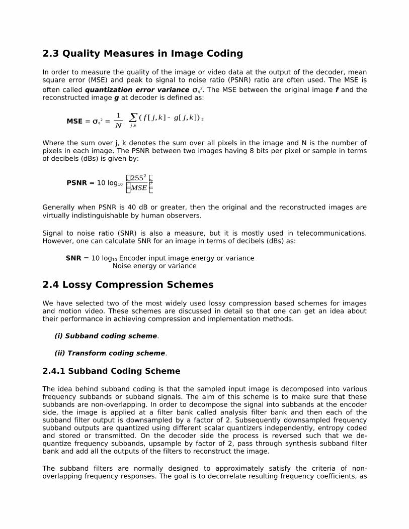
Figure 4.8 Comparison of image compression results using DCT and DWT ……….. 48Figure 4.9(a) Original Lena Image (256 x 256 Pixels, 24-Bit RGB)……………………….…. 50Figure 4.9(b) JPEG Compressed (Compression Ratio 43:1)…………………………………….…. 50Figure 4.9(c) JPEG2000 Compressed (Compression Ratio 43:1)………………………….……. 50Figure 4.10 A test image used to demonstrate the advantages of ROI coding………

51Figure 4.11(a) Compression with standard JPEG based on DCT…………………………….……

51 Figure 4.11(b) Compression with standard JPEG2000 based on DWT…………..…….……. 51Figure 4.12(a) Comparing resources of the FPGA used for DCT and DWT using

Xilinx’s Virtex-E series…………………………………………………………………………….53

Figure 4.12(b) Comparing resources of the FPGA used for DCT and DWT using Altera’s Apex20KE series …………………………………………………….…………..….

53Figure 4.13 Comparing resources of the ASIC used for DCT and DWT…………….……. 54Figure 4.14(a) Comparing data processing rates of DCT and DWT using Xilinx

and Altera’s FPGA………………………………………………………………………….………54

Figure 4.14(b) Comparing data processing rates of DCT and DWT using TSCM ASIC…………………………………………………………………………………………………….. 54Figure 5.1 The 8-ponit IDCT using Modified Loeffler Algorithm……………………………. 56Figure 5.2 The Butterfly……………………………………………………………………………………….…. 57Figure 5.3 The rotator…………………………………………………………………………………………….. 57Figure 5.4 Implementation of the rotator for IDCT…………………………………….…………. 57Figure 5.5 The 8-point DCT using Modified Loeffler Algorithm……………………………..

58Figure 5.6 The rotator for DCT………………………………………………………………………………..

58

Figure 5.7 Implementation of the rotator for DCT………………………………………………... 58Figure 5.8 Comparing different FPGA technologies with the clock frequencies used to implement 1-D 8-point DCT………………………………………………….... 68Figure 5.9 Comparing different FPGA technologies with the clock frequencies used to implement 1-D 8-point IDCT…………………………………………..…....

68Figure 5.10 Comparing different FPGA technologies to SIF frames processed per second using 2-D 8x8 DCT……………………………….……………….….…….… 69Figure 5.11 Comparing different FPGA technologies to SIF frames processed per second using 2-D 8x8 IDCT…………………………...………………………………. 69Figure 5.12 Comparing different FPGA technologies to CCIR-TV frames processed per second using 2-D 8x8 DCT………………………………………….…

69Figure 5.13 Comparing different FPGA technologies to CCIR-TV frames processed per second using 2-D 8x8 IDCT……………………………………..……. 70Figure 5.14 Comparing different FPGA technologies to HDTV frames processed per second using 2-D 8x8 DCT……………………………………………………………….

70Figure 5.15 Comparing different FPGA technologies to HDTV frames processed per second using 2-D 8x8 IDCT…………………………………………………………….

70

List of Tables Table 3.1 Statistical information of the reconstructed images using subband coding……………………………………………………….……………………

29Table 3.2 Statistical information of the reconstructed images using DCT/IDCT.… 32Table 3.3 Statistical information of the reconstructed images using JPEG……….… 33Table 3.4 Statistical information of the reconstructed images using EZW…………..

35Table 3.5 Statistical information of the reconstructed images using SPHIT……….. 38Table 4.1 Improvement in PSNR using DWT filter bank at S=3 over DCT based Haar transform……………………………………………………………………….……

43Table 4.2 Improvement in PSNR using DWT filter bank at S=4 over DCT based Haar transform……………………………………………………………….……………

44Table 4.3 Improvement in PSNR using DWT-JPEG over DCT-JPEG……………………... 45Table 4.4 PSNR corresponding to average MSE of all test images for each standard …………………………………………………………………………….……….…

46Table 4.5 Comparison of image compression results using DCT and DWT ……..….47Table 4.6 Performance comparisons of ZTE wavelet coder and MPEG-4’s DCT based coder …………………………………………………………………………………………..

49Table 4.7 Resources of the FPGAs used and data processing rates for DCT and DWT encoders………………………………………………………………………………………..

52Table 4.8 Resources of the ASIC used and data processing rate for DCT and

DWT encoders………………………………………………………………………………………… 53

Table 5.1 Resources of the Xilinx Virtex-II FPGA used for 8-point IDCT………………59

Table 5.2 Constraints and delays of the Xilinx Virtex-II FPGA used for 8-point IDCT…………………………………………………………………………..………………

60Table 5.3 Delays for processing one frame using 8X8 2-D IDCT……………….……..…

60Table 5.4 No. of frames processed and improvement using 8X8 2-D IDCT………… 61Table 5.5 Resources of the Xilinx Virtex-II FPGA used for 8-point DCT…………….…. 61Table 5.6 Constraints and delays of the Xilinx Virtex-II FPGA used for 8-point DCT….………………………..………………………………………………………….

62Table 5.7 Delays for processing one frame using 8X8 2-D DCT………………….…..….. 62Table 5.8 No. of frames processed and improvement using 8X8 2-D IDCT…………. 62Table 5.9 Resources of the Altera Acex-1K FPGA used for 8-point IDCT…….…….… 63Table 5.10 Constraints and delays of the Altera Acex-1K FPGA used

for 8-point IDCT…………………………………………………………………………………….…63

Table 5.11 Delays for processing one frame using 8X8 2-D IDCT…………………..…….. 63Table 5.12 No. of frames processed and improvement using 8X8 2-D IDCT..……... 64Table 5.13 Resources of the Altera Acex-1K FPGA used for 8-point DCT………….…..

64Table 5.14 Constraints and delays of the Altera Acex-1K FPGA used for 8-point DCT…………………………………………………………………….……….….……

64 Table 5.15 Delays for processing one frame using 8X8 2-D DCT………………………..…. 65Table 5.16 No. of frames processed and improvement using 8X8 2-D DCT………….. 65Table 5.17 Resources of the Lucent ORCA-3C/3T FPGA used for 8-point IDCT….…. 65Table 5.18 Constraints and delays of the Lucent’s FPGA used for 8-point IDCT…….66Table 5.19 Delays for processing one frame using 8x8 2-D IDCT……………………….…. 66Table 5.20 No. of frames processed and improvement using 8X8 2-D DCT……..…… 66Table 5.21 Resources of the Lucent ORCA-3C/3T FPGA used for 8-point DCT……….67Table 5.22 Constraints and delays of the Lucent’s FPGA used for 8-point DCT……..67Table 5.23 Delays for processing one frame using 8X8 2-D DCT…………………………... 67Table 5.24 No. of frames processed and improvement using 8x8 2-D DCT…………..

68

Chapter 1

Introduction

1.1 Background

Digital image compression is a very popular research topic in the field of multimedia processing. The major focus of research is to develop different compression schemes/algorithms in order to provide good visual quality and fewer bits to represent an image in digital format. These compression schemes are either implemented in software using higher-level languages such as C or Java or in hardware using application specific integrated circuit (ASIC). Although this hardware implementation speeds up image/video processing but ASIC is considered as an inflexible solution.

Recently reconfigurable devices namely field-programmable gate array (FPGA) have been introduced to implement compression schemes/algorithms in hardware to speed up image/video processing as a flexible and cost effective solution. Although current FPGA implementations based on discrete cosine transform (DCT) support video frame formats such as QCIF, SIF and CCIR-TV, but the author has taken following challenges to provide more improvement in digital image compression:

Is it possible to provide significant speed up for processing video frame formats such as SIF and CCIR-TV than the minimum required rates?

Is it possible to implement DCT based FPGA implementation even for HDTV video frame standard, which is still a major problem for the existing DCT based FPGA implementations?

1.2 Goals of the Thesis

This thesis describes the research and development author has done for his mater’s project and has two main goals.

The first is to compare the performance of image and video compression transforms in particular DCT and the discrete wavelet transform (DWT).

The second goal involves the hardware implementation of the DCT and the inverse discrete cosine transform (IDCT) for different FPGA technologies such as Xilinx, Altera and Lucent. The implementation provides video frame processing for frame formats such as SIF, CCIR-TV and HDTV.

1.3 Author’s Contribution to the Thesis

The author has contributed the following work as a part of research in image and video compression.

Generation of image compression results of standards/algorithms using subband coding, DCT and DWT based coding.

Literature survey of various research papers and websites to gather valuable data so that performance of DCT and DWT for image and video compression applications could be compared.

Simulation and synthesis of the currently known fastest 8-point 1-D DCT and IDCT algorithm for different FPGA technologies. This work also include results indicating improvement in video processing for frame formats such as SIF, CCIR-TV and HDTV, using 2-D 8x8 DCT/IDCT in FPGA.

1.4 Organization of the Thesis

This thesis is organized into five chapters. The aim is to present information in a concise and comprehensive manner so that the reader can understand necessary theoretical concepts and the practical work done by the author.

Chapter 2 gives an overview of image compression, classification of compression schemes and the definition of some widely used terms such as MSE, PSNR and SNR. It also provides the theoretical background of the lossy compression schemes. It discusses schemes like subband coding, discrete cosine transform (DCT), lapped transform (LT) and discrete wavelet transform based coding in detail.

Chapter 3 introduces the practical work done by the author. This chapter describes the image compression results of the standards/algorithms introduced in Chapter 2. Image and video compression software known as VcDemo has been used to generate these results. Chapter 4 describes the work done by the author to compare the performance of discrete cosine transform (DCT) and discrete wavelet transform (DWT). The author has gathered valuable data from various research papers and websites, and presented in a comprehensive way so that the reader can have more practical and in depth knowledge.

Chapter 5 describes the work done by the author to implement DCT and inverse discrete cosine transform (IDCT) in hardware for different FPGA technologies. This work is contributed to the previous chapter as the ease of implementing DCT both in software and hardware was highlighted in it. The author has implemented the 8-point 1-D DCT/IDCT modified Loeffler algorithm in VHDL using ModelSim and Leonardo-Spectrum software. The synthesis results are presented in detail including the ones indicating improvement in video processing for frame formats such as SIF, CCIR-TV and HDTV, using 2-D 8x8 DCT/IDCT in FPGA.

Chapter 6 gives the final conclusion of the thesis and presents some future work.

Chapter 2

Compression Schemes for Image Coding

2.1 Digital Image Compression

Digital image compression is a very popular research topic in the field of multimedia processing. Its goal is to store an image in a more compact form, i.e., a representation that requires fewer bits than the original image. It relies on the fact that image information, by its very nature, is not random but exhibits order and has some form of structure. If this order and structure can be extracted, the essence of the information often can be represented and transmitted using less data bits than would be needed for the original. We can then reconstruct the original or a close approximation of it at the receiving end.

Image, video and audio signals can be compressed due to the following reasons:

Within a single image or a single video frame, there exists significant correlation or redundancy among neighboring samples or pixels. This correlation is referred as spatial correlation or redundancy.

For data acquired from multiple sensors (such as satellite images), there exists significant correlation or redundancy among samples from these sensors. This correlation or redundancy is called spectral correlation or redundancy.

For temporal data (such as video sequence), there is significant correlation or redundancy among pixels of successive video frames. This is referred to as temporal correlation or redundancy.

A systematic view of the compression process is depicted in Figure 2.1.

ENCODER

Source

image data DECODER Source image data

Source Coder

Channel Coder

Source Decoder

Channel Decoder

Figure 2.1 Generic compression systems

As depicted in Figure 2.1, the source coder performs the compression process by reducing the input image data size to a level that can be supported by the storage or transmission channel. The output bit rate1 of the encoder is measured in bits per sample or bits per pixel. For image or video data, a pixel2 is the basic element, therefore bits per sample (bps) also referred to as bits per pixel (bpp). The channel coder translates the compressed bit-stream into a signal suitable for either storage or transmission using various methods such as variable length coding, Huffman coding or Arithmetic coding.

In order to reconstruct the image or video data the process is reversed at the decoder. In compression systems, the term ‘compression ratio’ is used to characterize the compression capability of the system.

Compression ratio = Source coder input data size Source coder output data size

For a still image, size could to the bits needed to represent the entire image. For video, size could refer to the bits needed to represent one frame of video, i.e., one second of video.

2.2 Classifying Compression Schemes

The classification of compression schemes can be done in the following manner.

(a) Lossless vs. Lossy compression: In lossless compression schemes the reconstructed image, after compression, is digitally identical to the original image. However, lossless compression can only achieve a modest amount of compression. On the other hand, lossy schemes are capable of achieving much higher compression but under normal viewing conditions no visible loss is perceived (visually lossless). Some of the lossy compression schemes used include differential pulse code modulation (DPCM), pulse code modulation (PCM), vector quantization (VQ), Transform and Subband coding. An image reconstructed following a lossy compression contains degradation relative to the original. Often this is because the compression scheme also discards non-redundant information.

(b) Predictive vs. Transform coding: In predictive coding, information already sent or available is used to predict other values, and the difference is coded. Since this is done in the image or spatial domain, it is relatively simple to implement and is readily adapted to local image characteristics. The DPCM is one particular example of predictive coding. Transform coding, on the other hand, first transforms the image from its spatial domain representation to a different type of representation using some well-known transforms such as DCT, DWT or Lapped transform, and then codes the transformed values (coefficients). This method provides greater data compression compared to predictive methods as transforms use energy compaction properties to pack an entire image or a video frame into fewer transform coefficients. Most of these coefficients become insignificant after applying quantization, which means less data to be transmitted. In predictive coding, the differences between the original image or video frame samples and the predicted ones remain significant even after applying quantization. This means more data to be transmitted compared to transform coding.

(c) Subband Coding: The fundamental concept behind subband coding is to split the frequency band of a signal (image in our case) in various subbands. To code each subband, we use a coder and bit rate accurately matched to the statistics of the subband.

1Normally the term bit rate in image compression is used in terms of bits per sample or bits per pixel. In case of transmitting data through communication channels we measure the bit rate in terms of bits per second.2In most literature the pixel is also referred to as pel.

2.3 Quality Measures in Image Coding

In order to measure the quality of the image or video data at the output of the decoder, mean square error (MSE) and peak to signal to noise ratio (PSNR) ratio are often used. The MSE is

often called quantization error variance q2. The MSE between the original image f and the

reconstructed image g at decoder is defined as:

MSE = q2 =

N

1

kj

kjgkjf,

]),[],[( 2

Where the sum over j, k denotes the sum over all pixels in the image and N is the number of pixels in each image. The PSNR between two images having 8 bits per pixel or sample in terms of decibels (dBs) is given by:

PSNR = 10 log10

MSE

2255

Generally when PSNR is 40 dB or greater, then the original and the reconstructed images are virtually indistinguishable by human observers.

Signal to noise ratio (SNR) is also a measure, but it is mostly used in telecommunications. However, one can calculate SNR for an image in terms of decibels (dBs) as:

SNR = 10 log10 Encoder input image energy or variance Noise energy or variance

2.4 Lossy Compression Schemes

We have selected two of the most widely used lossy compression based schemes for images and motion video. These schemes are discussed in detail so that one can get an idea about their performance in achieving compression and implementation methods.

(i) Subband coding scheme.

(ii) Transform coding scheme.

2.4.1 Subband Coding Scheme

The idea behind subband coding is that the sampled input image is decomposed into various frequency subbands or subband signals. The aim of this scheme is to make sure that these subbands are non-overlapping. In order to decompose the signal into subbands at the encoder side, the image is applied at a filter bank called analysis filter bank and then each of the subband filter output is downsampled by a factor of 2. Subsequently downsampled frequency subband outputs are quantized using different scalar quantizers independently, entropy coded and stored or transmitted. On the decoder side the process is reversed such that we de-quantize frequency subbands, upsample by factor of 2, pass through synthesis subband filter bank and add all the outputs of the filters to reconstruct the image.

The subband filters are normally designed to approximately satisfy the criteria of non-overlapping frequency responses. The goal is to decorrelate resulting frequency coefficients, as

non-overlapping frequency subbands are uncorrelated. It is this property that the subband filtering tries to achieve for perfect decorrelation. Subband filters are designed to be approximations to ideal frequency selective filters, where the combined response from all the filters covers the entire spectral band of the image. But in reality total decorrelation is never achieved since these filters only approximate ideal filters.

A general diagram to explain subband coding scheme is depicted in Figure 2.2. An input sampled image x(n) is applied on a bank of analysis filters and decomposed into M frequency subbands, each one downsampled by factor of 2 and encoded independently. Later we transmit or store this information. The decoder side performs the reverse process such that finally we add the synthesis filter bank output to reconstruct the image as x’(n). The difference between

x(n) and x’(n) will be considered MSE or q2.

Encoders Decoders

Original image x(n)

Bandpass analysis filter bank

Reconstructed image x’(n)

Bandpass synthesis filter bank

Figure 2.2 Subband coding scheme used for M-frequency subbands

The filters used in subband coding are known as quardrature mirror filters (QMF) such that we only have to design the low pass filter H() while the response of the high pass filter H(+) has additional phase shift of 180 degrees compared to the low pass filter. The accuracy of the filter depends upon number of filter coefficients or filter taps.

One of the methods in subband coding is to use octave tree decomposition of an image data into various frequency subbands. The idea is that we first we filter and decimate the image into lowest and high frequency subbands and later only decompose the lowest frequency subband

BP-0

BP-1

BP-M

2:1

2:1

2:1

En-0

En-1

En-M

Transm

ission or Storage

De-0

De-1

De-M

1:2

1:2

1:2

BP-0

BP-1

BP-M

output into further low and high frequency subbands followed by decimation. This technique is very popular and even used in wavelet transform based coders. The output of each decimated subband is quantized and encoded separately. The result of each subband will have a different quantizer, with each quantizer having its own separate rate (bits/sample).

It should be clear that subband coding itself doesn’t achieve compression. It merely decorrelates the original data and packs the image energy into various frequency subbands. It’s due to the result of decimation that reduces number subband coefficients in each subband, and later quantization that discards many coefficients (as they have small variances with respect to predefined threshold value) prior to encoding to give compression.

Figure 2.3 Octave tree subband decomposition

In practical 2-dimensional subband coding systems, we divide the 2-D spatial frequency domain of the original image into different subbands at any level. For example, in Figure 2.4 we decompose each of the two images into four subbands LL, HL, LH and HH at the first level.

Figure 2.4 Two-dimensional subband decomposition of images at first level

Disadvantages of Subband Coding

One of the major problems with the subband coding is to resolve the bit allocation problem or the number of bits assigned to each individual subband to get the best performance. One way is to use the idea of optimal bit allocation to each quantized subband output individually. This is mostly valid for higher bit rates of approximately 1 bit/sample or more.

We summarize some disadvantages of the subband coding scheme in the following.

Subband coding method is not able to determine optimal coding system for low bit rate applications.

The optimal bit allocation changes as overall bit rate changes, which requires that every time the coding process must be repeated in its entirety for each new desired target bit rate.

It is not possible to perfectly decorrelate all the frequency subbands, as the filters are not ideal and there is slight overlapping between adjacent frequency subbands. Hence there always exits a small correlation between adjacent frequency subbands, which is not desirable for compression.

Subband coding scheme is not useful in motion compensated video as its very difficult to perform motion estimation in frequency subbands without generating large prediction errors.

2.4.2 Transform Coding Scheme

A transform is a mathematical function that is used to convert one set of values to a different set and thereby creating a new way of representing the same information. All of the transforms we are going to discuss are lossless themselves; with sufficient arithmetic precision, the transforms can be reversed to any desired degree of accuracy. But the overall coding schemes are lossy due to quantization, which is applied to round off the values of transform coefficients.

We are going to discuss following transform based coding schemes used in image and video compression.

(a) Discrete Cosine Transform (DCT) based coding scheme.

(b) Lapped Transforms (LT) based coding scheme.

(c) Discrete Wavelet Transform (DWT) based coding scheme.

2.4.2.1 Discrete Cosine Transform (DCT) Based Coding Scheme

Discrete cosine transform1 (DCT) translates the image information from spatial domain to frequency domain to be represented in a more compact form. Its stochastic properties are similar to Fourier transform and considers the input image, audio or video signal to be a time invariant or stationary signal.

Before going into the details of DCT we will be discussing the fundamentals of Fourier transform, which forms the basis of DCT.

Fourier Transform (FT)

Fourier Transform (FT) is a reversible transform, i.e., it allows going reverse and forward between the raw (spatial or time domain) and the processed (transformed) signals. However, only either of them is available at any given time. This means no frequency information is available in the time-domain signal, and no time information is available in the Fourier transformed signal.

FT gives the frequency information of the signal, which means that it tells us how much of each frequency exists in the signal, but it does not tell us when in time these frequency components exist. This information is not required when the signal is so-called stationary. Signals whose frequency content does not change in time are called stationary signals. In other words, the frequency contents of stationary signals do not change in time. In that case, one does not need to know at what times frequency components exist since all frequency components exist at all times.

The FT and inverse FT for a continuous signal are defined as:

X(f) =

dtetx ftj2)(

x(t) =

dfefX ftj2)(

FT can be used for non-stationary signals, if we are only interested in what spectral components exist in the signal, but not interested where these occur. However, if this information is needed, i.e., if we want to know, what spectral component occur at what time (interval), then Fourier transform is not the right transform to use.

In order to obtain discrete Fourier transform (DFT), we simply replace the integration in FT’s mathematical expression by summation and calculate it over finite samples.

The kth DFT coefficient of a length N sequence or samples {x(n)} is defined as :

1 The discrete cosine transform (DCT) is a special case of discrete Fourier transform (DFT) in which the sine components have been eliminated leaving only the cosine terms.

X(k) =

1

0

)(N

n

knNWnx , k=0,………., N-1

Where, WN = e Nj /2 = cos (2/N) – j sin (2/N) is the Nth root of unity. The original sequence {x(n)} can be retrieved by the inverse discrete Fourier transform (IDFT) is

x(n) = N

1

1

0

)(N

k

knNWkX , n=0,………., N-1

Definition and Properties of DCT

The forward N-point one-dimensional DCT and inverse DCT can be defined as follows:

Forward N-point DCT = X(k) = N

2 ck

1

0 2

)12(cos)(

N

n N

knnx

, k= 0,1,………,N-1

Inverse N-point DCT = x(n) = N

2

1

0 2

)12(cos)(

N

kk N

knkXc

, n= 0,1,………,N-1

where ck =

0,1

0,2/1

k

k

Both DCT and IDCT are orthogonal, separable and real transforms. Being separable means that the multidimensional transform can be decomposed into successive application of one-dimensional transforms in the appropriate directions. Similarly orthogonal means if the matrices of DCT and IDCT are non-singular and real then their inverse is obtained merely by applying transpose operation. Like Fourier transform, DCT also considers the input sampled data to be a time invariant or stationary signal.

In case of image and video compression standards such as baseline JPEG and MPEG, 8-point DCT and IDCT are used. The image or each motion video frame of size NXN pixels is divided into two-dimensional non-overlapping blocks often called sub-images or basis functions of size 8x8 (having 64 pixels each) and 2-D DCT is applied on the encoder side, while on the decoding side 2-D IDCT is applied to recover the original data.

The 8-point 2-D DCT and IDCT to generate 8x8 data matrices are calculated as:

2-D DCT = Xk,l = 4

)()( lckc

7

0

7

0, 16

)12(cos

16

)12(cos

m nnm

lnkmx

where k,l = 0,1,………..,7

2-D IDCT= xm,n =

7

0

7

0lk,

16

1)l(2ncos

16

1)k(2mcosX

4

)()(

k l

lckc

where m,n = 0,1,………..,7

and c(k),c(l) =

otherwise

lk

,1

0&,2/1

One strategy to compute the 2-D DCT and IDCT is the standard row-column separation. The 2-D transform is performed by applying the 1-D transform to each row and subsequently to each column of the data matrix.

Relation to Karhunen-Loeve Transform (KLT)

The performance of DCT in decorrelating image signal is closer to Karhunen-Loeve transform (KLT). KLT is the most optimal block based transform for data compression in a statistical sense because it optimally decorrelates an image signal in the transform domain by packing the most information in a few coefficients and minimizes the mean square error between the reconstructed and original image compared to any other transform. However, KLT is constructed from the eigenvalues and the corresponding eigenvectors of a covariance matrix of the data to be transformed; it is signal dependent and there is no fast algorithm for its computation. In general there are several characteristics that are desirable in a transform when it is used for the purpose of data compression.

a) Data decorrelation: The optimal transform completely decorrelates the data in a sequence/block, i.e., it packs the most amount of energy in the fewest number of coefficients. In this way, many coefficients can be discarded after quantization and prior to encoding. It is important to note that the transform operation itself doesn’t achieve compression. It aims at decorrelationg the original data and compacting a large fraction of the signal energy into relatively fewer transform coefficients.

b) Data independent basis function: Due to large statistical variations in image or video data, the optimum transform usually depends on the data and finding the basis functions if such transform is computationally a very intensive task. This is particularly a problem if the data blocks are highly non-stationary, which forces to use more than one set of basis functions to achieve high decorrelation. Thus it is always desirable to trade optimum performance for a transform whose basis functions are data-independent.

c) Fast implementation: The number of operations required for an n-point transform is generally of the order O(n2). Some transforms have fast implementation, which reduce the number of operations to O(n log2 n), e.g., FFT. For a separable n x n 2-D transform such as DCT, performing the row and column 1-D transforms, successfully reduce the number of operations from O(n4) to O(2n2 log2 n).

The performance of DCT is very much near to the statistically optimal KLT because of its nice decorrelation and energy compaction properties. Moreover, as compared to KLT, DCT is data independent and many fast algorithms exist for its fast calculation so it is extensively used in multimedia compression standards.

DCT Based Image Compression/Decompression in Baseline JPEG

JPEG is the first established international digital compression standard for continuous-tone (multilevel) still images, both monochrome and color. Baseline JPEG is the simplest of all JPEG implementations based upon sequential processing mode (image is scanned from left to right and top to bottom) such that it uses 8-bit sample or pixel inputs for DCT based compression of 2-D 8 x 8 non-overlapping blocks in an image, followed by quantization of the DCT coefficients and entropy coding of the result.

RGB color images prior to compression are converted into a luminance component Y and two chrominance components U and V. The luminance component contains the shades of gray and is a monochrome image. Two chrominance components together contain the color information. Encoding and decoding operations in the baseline JPEG are performed for luminance and chrominance components.

The block diagrams of Baseline JPEG encoder and decoder are given in Figures 2.5 and 2.7.

Source image

Transmission or Storage of image data as file

Figure 2.5 Baseline JPEG encoder for image compression

Figure 2.6 Zigzag scan of DCT coefficients at encoder

Received or Stored I image data from file

Convert fromraster order to8x8 2-D blocks

Subtract 128 from each pixel’s value

2-D DCT8 x 8 transform

Scalar Quanti-zation

DC coefficientDPCM coding

AC coefficientszigzag scan

Entropy coding

Entropy decoding

DC coefficientDPCM decoding

AC coefficientsde-zigzag scan

Inverse Quanti-zation

2-D IDCT8 x 8 transform

Add 128 to each pixel’s intensity value

Reconstructed image

Figure 2.7 Baseline JPEG decoder for image decompression

The processing of the luminance component of an image using the above compression standard at encoding side can be explained as:

i) The source image is partitioned into non-overlapping 2-D blocks of 8x8, which are processed sequentially in a raster scan fashion, left to right and top to bottom. The pixels in each block are level shifted by subtracting a value of 128. Since we use the pixel values of range 0 to 255 (8-bit unsigned integer), applying DCT will generate AC coefficients in the range –1023 to +1023 and these may be represented by an 11-bit signed integer. The DC coefficient generated, however, would be in the range 0 to 2040, and this unsigned 11-bit integer value would require different handling in the software or hardware performing DCT and subsequent operations. To avoid this ambiguity, the value of 128 is subtracted from each pixel prior to DCT. This subtraction has no effect on the AC coefficients but shifts the DC coefficients into the same range so that all can be represented as 11-bit signed integers.

ii) On each 2-D block of 8x8, DCT is applied to generate an array of 2-D transformed coefficients, which are grouped into different basis functions. The coefficient with lowest spatial frequency and highest variance value is considered as DC coefficient and it is proportional to the average brightness of the whole 2-D 8x8 spatial block. The rest are considered AC coefficients. In principle, DCT introduces no loss to the source samples; it merely transforms them to a domain in which they can be more efficiently encoded.

iii) The 2-D DCT array of coefficients are quantized using uniform scalar quantizer, which means each coefficient is quantized individually and independently. The quantization is based on the properties of human visual system (HVS), i.e., visual perception is less sensitive to higher frequency coefficients and more to low frequency coefficients. Thus, the weighting factors are selected to produce coarser quantization of high frequency coefficients and finer quantization of the low frequency coefficients. The quantization table can be scaled to provide a variety of compression levels to achieve desired bit rate and quality of the images. The quantization of the AC coefficients produces many zeros, especially at higher frequencies. The rounding process used in quantization is lossy but it gives lot of compression.

iv) To take advantage of the coefficient quantized as zeros, the 2-D DCT array of quantized coefficients is reordered using a zigzag pattern to form a 1-D sequence. This rearranges the coefficients in approximately decreasing order of their average energies (but in order of increasing spatial frequencies) to create large runs of zero values. The DC coefficient is separated from the Ac coefficients and the sequence of DC coefficients (one from each block) is first coded using DPCM.

Convert from8x8 2-D blocks to raster order

v) The final step at the encoder is to use entropy coding such as Huffman coding on both AC and DC (DPCM coded before) coefficients to achieve extra compression and making them more immune to error.

At the decoder side, after the encoded bit stream is entropy decoded, the 2-D array of quantized DCT coefficients is recovered using de-zigzag, reordered and each coefficient is inverse quantized. The resulting array of coefficients is transformed back using 2-D inverse DCT and adding 128 to each pixel value to yield an approximation of the original 8x8 block or sub-image. The same quantization and entropy coding tables are used at the encoder and decoder side.

Each chrominance component of the color image is encoded in the same way as luminance except that it is down sampled by the factor of 2 or 4 in both horizontal and vertical directions prior to DCT. At the decoder side, the reconstructed chrominance component is bilinearly interpolated to the original size.

DCT Based Image Compression/Decompression in MPEG

MPEG standard is being used for the coding of audio, motion video and graphical applications. Since its first emergence in 1989 as MPEG-1, many new standards have emerged such as MPEG-2 and MPEG-4.

In general, MPEG describes various tools that may be used to perform compression and gives some examples of how these might be implemented. It defines the syntax of a compliant bit stream and the ways in which a decoder must interpret valid bit streams, those that conform to the defined syntax. Due to this all MPEG standards are generic, i.e., application independent. They don’t define standard encoder rather a valid encoder is any device that can be implemented in hardware and /or software producing syntactically correct bit stream. This results in the desired output if the bit stream is fed to a compliant decoder.

We will be discussing the encoder and decoder models used in MPEG-1 due to simplicity, which use DCT as a basic tool of achieving data compression.

MPEG-1 Video Standard

The MPEG-1 video-coding algorithm is a lossy compression scheme that can be applied to a wide range of input formats and applications. However, it has been optimized for applications that support a continuous transfer rate of 1.5Mbits/sec (such as CD-ROM). In order to achieve more compression and need for random-access capability, MPEG-1 uses a combination of intraframe and interframe coding techniques. Also to improve compression ratio, it proposed using both predictive and interpolative coding schemes.

Compression functions within MPEG include the following:

a) Sample rate reduction in the spatial and temporal domains of both the luminance and the chrominance components.

b) Block-based DCT for the interframes and interframes.

c) Block-based motion compensation for predictive and interpolative frames.

d) Huffman entropy coding for the lossless compression of motion vectors and the quantized DCT coefficients.

Any color video format can be represented as combination of luminance component Y and two chrominance components U and V respectively. In MPEG-1, these color components are always interleaved and a macro-block is defined as the minimum coded unit consisting of four 2-D 8x8 blocks of luminance Y, one 8x8 block of U and one 8x8 block of V. Each macro-block is DCT coded, the DCT coefficients are quantized, coded using entropy coding and stored in output buffer of the encoder. Within a macro-block, processing is performed on 8x8 blocks.

In the encoder, the motion predictor compares the frames being coded to a reference frame. When a match is found, a motion vector is generated, specifying the location in the reference frame of the macro-block, or the block of residuals formed by subtracting the predicting macro-block is passed to the spatial encoder. This spatial encoder is similar to Baseline JPEG encoder but with the addition of a rate-control loop. Motion vectors are coded in a manner similar to that used for DC transform coefficients, i.e., DPCM coded. In the decoder, the data is decoded in the reverse way and the reconstructed video frames are obtained.

We show simplified MPEG-1 encoder and decoder in Figures 2.8 and 2.9.

Scale factor

Video Data In +

-

Prediction

+ Encoded data out

+

Framereorder

Motionpredictor

2-D DCT8 x 8 transform

ScalarQuantization+ Entropy

Coding

Trans-missionBuffer

RateControl

Dequantiza-tion

2-D IDCT8 x 8 transformReference

Frame

Predictionencoder

+

Motion Vectors

Figure 2.8 Simplified MPEG-1 encoder for video compression

Encoded Data In +

+

Video Out

DC Coefficients

Figure 2.9 Simplified MPEG-1 decoder for video decompression

Disadvantages of DCT

The major disadvantages of DCT are presented to indicate its limitations in multimedia applications.

In JPEG as well as MPEG, we divide an image or a video frame into 2-D non-overlapping blocks of 8x8 and apply 8-point 2-D DCT on them to obtain fewer transformed coefficients. But in these schemes only spatial correlation of the pixels inside the single 2-D block is considered and the correlation from the pixels of the neighboring blocks is neglected.

Since the blocks are non-overlapping, there may be discontinuities along the boundary regions of the blocks. Due to this it is not possible to completely decorrelate the blocks at their boundaries using DCT.

When DCT based block-coding schemes are used for compressing images or video frames, undesirable blocking artifacts affect the reconstructed images or video frames. This problem becomes severe under high compression ratios or very low bit rates.

2.4.2.2 Lapped Transforms (LT) Based Coding Scheme

The lapped transforms were developed specifically to solve the blocking effect inherent in DCT based coding schemes. Instead of non-overlapping 2-D blocks, they use the idea of overlapping

EntropyDecoder

Dequantiza-tion

2-D IDCT8 x 8 transform

FrameReorder

MotionPredictor

PredictionDecoder

Referenceframe store

+

2-D blocks of an image spatially. One of the special types of lapped transforms is called lapped orthogonal transform (LOT).

For image coding applications, the LOT basis functions are designed to resemble the DCT basis functions and thus, the behavior of lapped orthogonal transform coefficients is very similar to that of DCT coefficients. This means that DCT quantization and entropy coding strategies will work in LOT based encoding of images as well.

While it is true that blocking effects are reduced in LOT compressed images, other artifacts tend to appear, such as increased ringing around edges due to longer basis functions. The LOT represents an elegant extension of DCT for still image compression but due to its complexity in implementation as compared to the amount of improvement it provides, so far LOT has found less attraction for VLSI implementations.

2.4.2.3 Discrete Wavelet Transform (DWT) Based Coding Scheme

Over the past several years, the wavelet transform has gained widespread acceptance in signal processing in general, and in image compression research in particular. In applications such as still image compression, discrete wavelet transform (DWT) based schemes have outperformed other coding schemes like the ones based on DCT. Since there is no need to divide the input image into non-overlapping 2-D blocks and its basis functions have variable length, wavelet-coding schemes at higher compression ratios avoid blocking artifacts. Because of their inherent multiresolution nature, wavelet-coding schemes are especially suitable for applications where scalability and tolerable degradation are important. Recently the JPEG committee has released its new image coding standard, JPEG-2000, which has been based upon DWT.

Before going into the detail of some DWT based schemes, fundamentals of wavelet transform are discussed to give idea about its properties and usefulness for various applications.

Wavelet Transform (WT)

Basically we use wavelet transform (WT) to analyze non-stationary signals, i.e., signals whose frequency response varies in time, as Fourier transform (FT) is not suitable for such signals.

To overcome the limitation of FT, short time Fourier transform (STFT) was proposed. There is only a minor difference between STFT and FT. In STFT, the signal is divided into small segments, where these segments (portions) of the signal can be assumed to be stationary. For this purpose, a window function "w" is chosen. The width of this window in time must be equal to the segment of the signal where its still be considered stationary. By STFT, one can get time-frequency response of a signal simultaneously, which can’t be obtained by FT. The short time Fourier transform for a real continuous signal is defined as:

X(f,t) =

dtetwtx ftj 2* ])()([

Where the length of the window is (t-) in time such that we can shift the window by changing

value of t, and by varying the value we get different frequency response of the signal segments.

The Heisenberg uncertainty principle explains the problem with STFT. This principle states that one cannot know the exact time-frequency representation of a signal, i.e., one cannot know what spectral components exist at what instances of times. What one can know are the time

intervals in which certain band of frequencies exists and is called resolution problem. This problem has to do with the width of the window function that is used, known as the support of the window. If the window function is narrow, then it is known as compactly supported. The narrower we make the window, the better the time resolution, and better the assumption of the signal to be stationary, but poorer the frequency resolution:

Narrow window ===> good time resolution, poor frequency resolution Wide window ===> good frequency resolution, poor time resolution

The wavelet transform (WT) has been developed as an alternate approach to STFT to overcome the resolution problem. The wavelet analysis is done such that the signal is multiplied with the wavelet function, similar to the window function in the STFT, and the transform is computed separately for different segments of the time-domain signal at different frequencies. This approach is called multiresolution analysis (MRA), as it analyzes the signal at different frequencies giving different resolutions.

MRA is designed to give good time resolution and poor frequency resolution at high frequencies and good frequency resolution and poor time resolution at low frequencies. This approach is good especially when the signal has high frequency components for short durations and low frequency components for long durations, e.g., images and video frames.

The wavelet transform involves projecting a signal onto a complete set of translated and dilated

versions of a mother wavelet (t). The strict definition of a mother wavelet will be dealt with later so that the form of the wavelet transform can be examined first. For now, assume the

loose requirement that (t) has compact temporal and spectral support (limited by the uncertainty principle of course), upon which set of basis functions can be defined.

The basis set of wavelets is generated from the mother or basic wavelet is defined as:

a,b(t) =

a

bt

a

1 ; a, b 1 and a>0

The variable ‘a’ (inverse of frequency) reflects the scale (width) of a particular basis function such that its large value gives low frequencies and small value gives high frequencies. The variable ‘b’ specifies its translation along x-axis in time. The term 1/ a is used for normalization. The 1-D wavelet transform is given by:

Wf (a,b) =

dtttx ba )()( ,

The inverse 1-D wavelet transform is given by:

x(t) =

02, )(),(

1

a

dadbtbaW

C baf

where C =

d2

)<

1 ‘’ refers to set of real numbers

() is the Fourier transform of the mother wavelet (t). C is required to be finite, which leads to one of the required properties of a mother wavelet. Since C must be finite, then (0) 0 to

avoid a singularity in the integral, and thus the (t) must have zero mean. This condition can be stated as

dtt)( = 0

and known as the admissibility condition.

The other main requirement is that the mother wavelet must have finite energy:

dtt2

)( <

A mother wavelet and its scaled versions are depicted below indicating the effect of scaling.

Figure 2.10 Mother wavelet and its scaled versions

Unlike the STFT which has a constant resolution at all times and frequencies, the WT has a good time and poor frequency resolution at high frequencies, and good frequency and poor time resolution at low frequencies.

Now we discuss discrete wavelet transform (DWT), which transforms a discrete time signal to a discrete wavelet representation. The first step is to discretize the wavelet parameters, which reduce the previously continuous basis set of wavelets to a discrete and orthogonal / orthonormal set of basis wavelets.

m,n(t) = 2m/2 (2mt – n) ; m, n 1 such that - < m, n <

1 ‘’ refers to the set of integers.

The 1-D DWT is given as the inner product of the signal x(t) being transformed with each of the discrete basis functions.

Wm,n = < x(t), m,n(t) > ; m, n Z

The 1-D inverse DWT is given as:

x(t) = m n

nmnm tW )(,, ; m, n Z

The next step toward developing a DWT is to be able to transform a discrete time signal. The wavelet transform can be interpreted as a applying a set of filters. Digital filters are very efficient to implement and thus provide us with the needed tool for performing the DWT, and are usually applied as equivalent low and high-pass filters. The design of these filters is similar to subband coding, i.e., only the low pass filter has to be designed such that the high pass filter has additional phase shift of 180 degree as compared to the low pass filter. Unlike subband coding, these filters are designed to give flat or smooth spectral response and are bi-orthogonal.The generic form of 1-D DWT is depicted in Figure 2.11. Here a discrete signal is passed through a lowpass and highpass filters H and G, then down sampled by a factor of 2, constituting one level of transform. The inverse transform is obtained by up sampling by a factor of 2 and then using the reconstruction filters H’ and G’, which in most instances are the filters H and G reversed.

Figure 2.11 Perfect reconstruction filter bank for used for 1-D DWT

The 1-D DWT can be extended to 2-D transform using separable wavelet filters. With separable filters, applying a 1-D transform to all the rows of the input and then repeating on all of the columns can compute the 2-D transform. When one-level 2-D DWT is applied to an image, four transform coefficient sets are created. As depicted in Figure 2.12, the four sets are LL, HL, LH, and HH, where the first letter corresponds to applying either a low pass or highpass filter to the rows, and the second letter refers to the filter applied to the columns.

Figure 2.12 Level one 2-D DWT applied on an image

Figure 2.13 (a) Level-3 dyadic DWT scheme used for image compression

Figure 2.13(b) Level-3 dyadic DWT scheme used for image compression

Compression Algorithms Using DWT

The wavelet based coding has improved significantly since the introduction of Baseline JPEG in 1992. Early wavelet coders had performance that was at best comparable to transform coding using DCT. Also, these early wavelet coders were designed using the same techniques applied to subband coding. A real breakthrough in wavelet transform based coding was the introduction of embedded zero-tree (EZW) coding.

The EZW algorithm was able to exploit the multi-resolution properties of the wavelet transform to give computationally less complex algorithm with very good performance. Improvement and enhancement to EZW have resulted in similar algorithms such as set partitioning in hierarchical trees (SPIHT) and zero-tree entropy (ZTE) coding.

Recently a new algorithm used for constituting integer wavelet transform, known as lifting scheme (LS) has been proposed. Bi-orthogonal wavelet filters using this scheme have been

identified as very nice for lossy image compression applications. We will be discussing some of the following algorithms:

a) EZW Algorithm

b) SPHIT Algorithm

c) ZTE Algorithm

a) Embedded Zero-Tree Wavelet (EZW) Algorithm

This algorithm laid the foundation of modern wavelet coders and provides excellent performance for the compression of still images as compared to block based DCT algorithm. Introduced by Shapiro [1] in 1993, this algorithm uses the multi-resolution properties of wavelet transform.

As the name implies, embedded means the encoder can stop encoding of image data at any desired target rate. Similarly, the decoder can stop decoding at any point resulting in image quality produced at the truncated bit stream of the image data. While the zero-tree structure is analogous to the zigzag scanning of the transform coefficients and end of block (EOB) symbol used in DCT based algorithms.

The EZW algorithm first uses DWT for the decomposition of an image where at each level i, the lowest spatial frequency subband is split into 4 more subbands for next higher level i+1,i.e., LLi+1, LHi+1, HLi+1 and HHi+1 and then decimated. The algorithm uses the idea of significance map as an indication of whether a particular coefficient is zero or nonzero (i.e., significant) relative to a given quantization level. This means that if a wavelet coefficient at a coarse scale or highest level is insignificant (quantized to zero) with respect to a given threshold T, then all wavelet coefficients of the same orientation at the same spatial location at next finer scales (i.e., lower level) are likely to be zero with respect to T. The coefficient at coarse scale is called parent while the coefficients at the next fine scales in the same spatial orientation are called children.

Figure 2.14 Parent-child dependencies of subbands in EZW

One can use this principle and code such a parent as a zero-tree root (ztr), thereby avoiding coding all of its children. This gives considerable compression as compared to block based coding algorithms such as DCT.

EZW scans wavelet coefficients subband by subband in a zigzag manner. Parents are scanned before any of their children by first scanning all neighboring parents. Each coefficient is compared against the current threshold T. A coefficient is significant if its amplitude is greater than T; such a coefficient is then encoded using one of the symbols negative significant (ns) or positive significant (ps). The zero-tree root (ztr) symbol is used to signify a coefficient below T, with all its children in the zero-tree data structure also below T. The isolated zero (iz) symbol signifies a coefficient below T, but with one of its child not below T.

For significant coefficients, EZW further encodes coefficient values using successive approximation quantization (SAQ) scheme. Coding is done bit-plane by bit-plane. The successive approximation approach to quantization of the wavelet coefficients leads to the embedded nature of EZW coded bit-stream. Finally the coefficients in the bit-stream are coded losslessly using adaptive arithmetic coding.

b) Set Partition In Hierarchical Tree (SPHIT) Algorithm

The SPHIT algorithm is a highly refined version of EZW algorithm. It was designed and introduced by Said and Pearlman [2] for still image compression. It can perform better at higher compression ratios for a wide variety of images than EZW. The term hierarchical trees refer to the quad-trees consisting of parents and children as defined in EZW. Set partitioning refers to the way these quad-trees partition the wavelet transform values at given threshold. For more detail study of this algorithm please refer to the reference.

c) Zero-Tree Entropy (ZTE) Coding Algorithm

ZTE coding is a new efficient technique for coding wavelet transform coefficients of motion-compensated video residuals or of video frames [3]. The technique is based on, but differs significantly from, the EZW algorithm. Like EZW, this new ZTE algorithm exploits the self-similarity inherent in the wavelet transform of images and video residuals to predict the location of information across wavelet scales.

ZTE coding organizes quantized wavelet coefficients into wavelet trees and then uses zero-trees to reduce the number of bits required to represent those trees. ZTE differs from EZW in four major ways: 1) quantization is explicit instead of implicit and can be performed distinct from the zero-tree growing process or can be incorporated into the process, thereby making it possible to adjust the quantization according to where the transform coefficient lies and what it represents in the frame; 2) coefficient scanning, tree growing, and coding are done in one pass instead of bit-plane-by-bit-plane; 3) coefficient scanning is changed from subband by subband to a depth-first traversal of each tree; and 4) the alphabet of symbols for classifying the tree nodes is changed to one that performs significantly better for low bit-rate encoding of video. The ZTE algorithm does not produce an embedded bit-stream as EZW does, but by sacrificing the embedding property, this scheme gains flexibility and other advantages over EZW coding, including substantial improvement in coding efficiency.

Figure 2.15 Reorganization of a wavelet tree into a wavelet block

In ZTE coding, the coefficients of each wavelet tree are reorganized to form a wavelet block as depicted in Figure 2.15. Each wavelet block comprises those coefficients at all scales and orientations that correspond to the frame at the spatial location of that block. The concept of the wavelet block provides an association between wavelet coefficients and what they represent spatially in the frame.

EZW scans coefficients from subband by subband in a zigzag manner. In ZTE, all wavelet coefficients that represent a given spatial block are scanned, in ascending frequency order from parent to child, to grandchild, and so on, before the coefficients of the next adjacent spatial location are scanned.

DWT Based Image Compression/Decompression in JPEG 2000

JPEG 2000 is the new ISO/ITU-T standard for still image coding. It is based on the discrete wavelet transform (DWT), scalar quantization, context modeling, arithmetic coding and post-compression rate allocation. The DWT is dyadic and can be performed with either the reversible filters, which provide for lossless coding, or the non-reversible bi-orthogonal ones, which provide for higher compression but not lossless. The quantizer follows an embedded dead-zone scalar approach and is independent for each sub-band.

Each sub-band is divided into rectangular blocks (called code-blocks in JPEG 2000), typically 64x64, and entropy coded using context modeling and bit-plane arithmetic coding. The coded data is organized in so called layers, which are quality levels, using the post-compression rate allocation and output to the code-stream in packets.

The fact that the subbands are encoded bit-plane-by-bit-plane makes it possible to select regions of the image that will precede the rest of the image in the code stream. By scaling the sub-band samples so that the bit-planes encoded first only contain ROI information and following bit-planes only contain background information. The only thing the decoder needs to receive is the factor by which the samples were scaled. The decoder can then invert the scaling based only on the amplitude of the samples. Other supported functionalities are error-resilience, random access, multi-component images, palletized color, compressed domain lossless flipping and simple rotation, to mention a few.

Figure 2.16 General block diagram of the JPEG 2000 (a) encoder and (b) decoder

The generic block diagram of the JPEG 2000 standard [4] depicted above seems like the one used for conventional JPEG, there are radical differences in all of the functionalities of each block of the diagram. They perform in a different manner compared to normal JPEG blocks by following the encoding procedure explained above.

DWT Based Image Compression/Decompression in MPEG-4 VTC

MPEG-4 visual texture coding (VTC) is the algorithm used in MPEG-4 to compress visual textures and still images, which are then used in photo realistic 3D models, animated meshes, etc., or as simple still images. It is based on the discrete wavelet transform (DWT), scalar quantization, zero-tree coding and arithmetic coding. The DWT is dyadic and uses a bi-orthogonal filter.

The quantization is scalar and can be of three types: single (SQ), multiple (MQ) and bi-level (BQ). With SQ each wavelet coefficient is quantized once, the produced bit-stream not being SNR scalable. With MQ a coarse quantizer is used and this information coded. A finer quantizer is then applied to the resulting quantization error and the new information coded. This process can be repeated several times, resulting in limited SNR scalability. BQ is essentially like SQ, but the information is sent by bit-planes, providing general SNR scalability.

Two scanning modes are available: tree-depth (TD), the standard zero-tree scanning, and band-by-band (BB). Only the latter provides for resolution scalability. The produced bit-stream is resolution scalable at first, if BB scanning is used, and then SNR scalable within each resolution level, if MQ or BQ is used. A unique feature of MPEG-4 VTC is the capability to code arbitrarily shaped objects. This is accomplished by the means of a shape adaptive DWT and MPEG-4’s shape coding. Several objects can be encoded separately, possibly at different qualities, and then decoded separately at the decoder to obtain the final decoded image. On the other hand, MPEG-4 VTC does not support lossless coding.

Disadvantages of DWT

Two major disadvantages of DWT are presented to indicate its limitations in multimedia applications.

The cost of computing DWT as compared to DCT is much higher. The complexity of calculating DWT depends upon the length of wavelet filter, which is at least one multiplication per coefficient.

The use of larger DWT basis functions or wavelet filters produces blurring and ringing noise near edge regions in images or video frames.

2.5 Conclusion

In this chapter we have described compression schemes used for image coding. First, we have introduced the concept of digital image compression and later classified different compression schemes. Lossy compression schemes namely subband coding and transform coding, have been discussed in detail. The transform coding schemes discussed are discrete wavelet transform (DCT), lapped transform (LT) and discrete wavelet transform (DWT). The DCT is a part of JPEG and MPEG compression standards and its stochastic properties are based upon Fourier transform (FT). Due to the complexity in implementation compared to the amount of improvement it provides, LT is not a popular transform. The DWT has better stochastic properties and has outperformed DCT providing higher image compression ratios. Both MPEG-4 (VTC) and JPEG 2000 use DWT for the compression of still images.

Chapter 3

Image Coding Using VcDemo

In this chapter, we show the results of various image compression standards/algorithms discussed in the previous chapter. We used the VcDemo software [5] to generate image-coding results to see the performance in terms of perceptual quality1, SNR and PSNR of the reconstructed images. As we have indicated in Chapter 2, PSNR is one of the widely used criteria in image and video compression than SNR as the latter is mostly used in telecommunications. The statistical information of the reconstructed images using each of these standards/algorithms is mentioned in separate tables. It should be clear that for encoding and decoding image data, lossless entropy coding (giving zero-channel error) is used and factors like MSE or quantization error (difference between variance of original image and the reconstructed one) is used to calculate PSNR of the reconstructed images. Due to quantization applied at encoding, the reconstructed or compressed image has less variance then the original one in order to achieve compression.

3.1 Subband Coding

We consider original 8-bit 256x256 “Lena” image as depicted in Figure 3.1(a) as our reference image. The compression rates used indicate the performance of this scheme.

1 Perceptual quality is measured according to the sensitivity/sharpness of a human eye to see details in an image and it varies for each person.

Figure 3.1(a) An 8 bps 256x256 uncompressed image of ” Lena “

From the options given for subband coding, we select the one to decompose the original image into subband images using QMF filters as depicted in Figure 3.1(b). We use level-2 subband image decomposition but one can increase or decrease the level of subband decomposition to generate subband images. This can affect both SNR and PSNR of the reconstructed images at higher compression rates. All the decomposed subband images are down sampled by a factor of 2 automatically. The QMF filters selected in this case have a length of 8 filter coefficients or taps. The length of these filters can be increased or decreased but has negligible influence on SNR and PSNR of the reconstructed images for using 12 or more filter coefficients. Looking at Figure 3.1(b), we can see the lowest frequency subband image located on the top left side. The other 6 decimated subband images in gray color represent high frequencies. There are in total 7 subband images generated after applying level-2 subband decomposition. These 7 subband images are quantized and entropy coded at 1 bps as depicted in Figure 3.1(c). After applying quantization at bit rate of 1 bps some of the high frequency subband images become zero and are not encoded. This is because high frequencies have less variance or energy than the lower frequencies in an image.

(b) (c)

Figure 3.1(b) Decomposition of “Lena” using level-2 subband decomposition (c) No. of subband images left after quantization and entropy coding at 1.0 bps

We reconstruct the “Lena” image at 1 bps in Figure 3.1(d) using entropy decoding and de-quantization of the Figure 3.1(c) subbands images and same QMF filters. We repeat the compression/decompression of “Lena” image for other bit rates using QMF filters having 8 taps or filter coefficients. As seen in Figure 3.1(e) and Figure (g), after applying quantization at low bit rates we get less encoded subband images. This affects the SNR, PSNR and visual quality of the reconstructed images depicted in Figures 3.1(f) and 3.1(h).

(d) (e)

Figure 3.1(d) Reconstructed image of “Lena” at 1 bps (e) No. of subband images left after quantization and entropy coding at 0.50 bps

(f) (g)

Figure 3.1(f) Reconstructed image of “Lena” at 0.50 bps (g) No. of subband images left after quantization and entropy coding at 0.25 bps

Figure 3.1(h) Reconstructed image of “Lena” at 0.25 bps

As we see that reconstructed “Lena” images using compression rates below 1 bps show artifacts, which are much more visible in the image reconstructed at 0.25 bps.

Original uncompressed image bit rate 8 bps

Total variance of the 7 decimated subband images

619.63

Compression rates used for coding 1 bps 0.50 bps 0.25 bps

Mean square error of reconstructed images at different compression rates

40 84.70 148.70

SNR in dBs of reconstructed images 18.40 15.10 12.60

PSNR in dBs of reconstructed images 32.10 28.90 26.40

Table 3.1 Statistical information of the reconstructed images using Subband coding

As indicated in Table 3.1 the original image in Figure 3.1(a) has bit rate of 8 bps. After applying level-2 subband decomposition, the total variance of the 7 subband images depicted in Figure 3.1(b) is computed as 619.63. We also mention the MSE, SNR and PSNR of the reconstructed images at different compression rates.

3.2 DCT Coding

In order to see the effectiveness of block based coding, we produce image compression results using DCT and IDCT. We compress the “Lena” image depicted in Figure 3.1(a) by selecting the option to apply 2-D DCT transform. The size of the block is selected as 8x8 but one can select other sizes available in the option. This can affect both SNR and PSNR of the reconstructed images. The DCT coefficients generated using 8x8 2-D DCT represent different spatial frequencies of the image. They are grouped into 64 basis functions or sub-images based upon their spatial frequencies depicted in Figure 3.2(a). The lowest frequency DCT coefficients are grouped into top left basis function while the high frequency coefficients are grouped into other

63 basis functions. The basis functions containing high frequency DCT coefficients have gray color for visibility. These basis functions are quantized and entropy coded at different compression rates.

As depicted in Figures 3.2(b), after applying quantization some of the high frequency basis function become zero and are not encoded at bit rate of 1bps. The reconstructed image using these quantized and entropy coded basis functions is depicted in Figure 3.2(c). It uses entropy decoding, de-quantization and 8x8 2-D IDCT transform.

(a) (b)

Figure 3.2(a) Decomposition of “Lena” image into 64 DCT basis functions (b) No. of DCT basis functions left after quantization and entropy coding at 1 bps

As we increase the compression rates, number of DCT basis functions left after quantization at these rates decrease. It means fewer basis functions are to be entropy coded as depicted in Figures 3.1 (d) and 3.1(f). This affects the SNR, PSNR and visual quality of the reconstructed images depicted in Figures 3.1 (d) and 3.1(g) respectively. It should be mentioned that high frequency DCT coefficients have less energy or variance as compared to low frequency DCT coefficients.

(c) (d)

Figure 3.2(c) Reconstructed image of “Lena” at 1 bps (d) No. of DCT basis functions left after quantization and entropy coding at 0.50 bps

(e) (f)

Figure 3.2(e) Reconstructed image of “Lena” at 0.50 bps (f) No. of DCT basis functions left after quantization and entropy coding at 0.25 bps

Figure 3.2(g) Reconstructed image of “Lena” at 0.25 bps

All the relevant information of the reconstructed images at different compression rates using 8x8 2-D DCT/IDCT is given in Table 3.2. The original image in Figure 3.1 has bit rate of 8 bps. The 64 DCT basis functions depicted in Figure 3.2(a) have total variance of 1148.76. The MSE, SNR and PSNR of the reconstructed images at different compression rates are also given. The reconstructed “Lena” images using compression rates below 1 bps show blocking artifacts, which are much more visible at 0.25 bps similar.

Original uncompressed image bit rate

8 bps

Total variance of the 64 sub-images or basis functions

1148.76

Compression rates used for coding 1 bps 0.50 bps 0.25 bps

Mean square error of reconstructed images at different compression rates

36.4 82.8 156.1

SNR in dBs of reconstructed images 18.8 15.2 12.4

PSNR in dBs of reconstructed images 32.5 29 26.2

Table 3.2 Statistical information of the reconstructed images using DCT/IDCT

3.3 JPEG Coding

We use 8x8 2-D DCT/IDCT based JPEG still image-coding standard to show its performance for “Lena “ image shown in Figure 3.1(a). First we select ITU-T Rec. T.81 (1994) standardized 8x8 luminance quantization matrix from the option to perform quantization of the DCT transform coefficients. Other 8x8 quantization matrices such chrominance, flat and high-emphasis are also available. The selection is made after checking the performance of other 8x8 quantization matrices to reduce quantization error and increase SNR and PSNR of the reconstructed images. Next we select optimal variable length coding (VLC) instead of standard variable length coding and fixed length coding (FLC) to have better coding efficiency and higher SNR and PSNR of the reconstructed images. The optimized quality factor for the reconstructed images is adjusted automatically according to the compression rates used. The reconstructed images at different compression rates are depicted in Figures 3.3(a), (b) and (c).

(a) (b)

Figure 3.3 Reconstructed images of “Lena” at (a) 1.0 bps (b) 0.50 bps

Figure 3.3(c) Reconstructed image of “Lena” at 0.30 bps

We summarize all information related to the reconstructed images using JPEG in Table 3.3. Most of information is similar to the one mentioned for simple 2-D DCT/IDCT except the optimal quality factor of the reconstructed images, which is an added feature of JPEG. As said before that it is adjusted automatically with the compression rate used. The results in the table show that JPEG is better than subband coding and simple 2-D 8x8 DCT/IDCT in terms of SNR and PSNR.

Original uncompressed image bit rate

8 bps

Compression rates used for coding 1 bps 0.50 bps 0.30 bps

optimized quality factor 57 19 9

Mean square error of reconstructed images at different compression rates

29.2 68.5 120.2

SNR in dBs of reconstructed image 19.7 16 13.6

PSNR in dBs of reconstructed image 33.5 29.8 27.3

Table 3.3 Statistical information of the reconstructed images using JPEG

3.4 EZW Coding

We perform compression using wavelet based EZW algorithm on the original 8-bit 256x256 “Lena” image depicted in Figure 3.1(a). First we perform level-7 dyadic decomposition of the image using DWT to generate wavelet sub-images as depicted in Figure 3.4(a). The level of decomposition can be changed, which can affect both SNR and PSNR of the reconstructed images. The decomposition is done before applying EZW coding algorithm and is similar to subband coding except that the filters used have different spectral response. In Figure 3.4(a), the lowest frequency wavelet coefficients are located in the very small top left wavelet sub-image. As we mentioned in chapter 2, EZW enables us to encode and decode an image at any target bit rate. We can select from the options to have similar or different encoding and

decoding bit rates for the “Lena” image at the same time. In our case we give similar encoding and decoding bit rates to have maximum SNR and PSNR of the reconstructed images. The EZW encoded wavelet sub-images are decoded at compression rates such as 1, 0.50 and 0.30 bps as depicted in Figures 3.4(b), (d) and (f). Note that after entropy decoding and de-quantization, there are lots of high frequency wavelet sub-images available. This is because the threshold for quantization and de-quantization is not fixed like subband coding and adjusted according to the scanning method used by EZW. In principle, EZW implements successive approximation quantization (SAQ) through a multipass scanning of the wavelet coefficients using successively decreasing thresholds. The advantage of EZW is the maintenance of high compression rates at the encoder side and after decoding large number of wavelet coefficients are available to reconstruct the images. In schemes like subband coding less frequency subband are available to reconstruct images after decoding at higher compression rates. The reconstructed images after EZW decoding are depicted in Figures 3.4(c), (e) and (g).

(a) (b)

Figure 3.4(a) Wavelet sub-images generated by applying level-7 dyadic DWT decomposition on “Lena” (b) Wavelet sub-images encoded at 1 bps and decoded at 1 bps using EZW

(c) (d)

Figure 3.4(c) Reconstructed image of Lena at 1.0 bps (d) Wavelet sub-images encoded at 0.50 bps and decoded at 0.50 bps using EZW

Looking at the reconstructed images, one can easily find the good perceptual quality even at low bit rates. Also the SNR and PSNR are higher than all the previous techniques we have discussed so far. As we said in the previous chapter that EZW was the real breakthrough in DWT based coding.

(e) (f)

Figure 3.4(e) Reconstructed image of “Lena” at 0.50 bps (f) Wavelet sub-images encoded at 0.30 bps and decoded at 0.30 bps using EZW

Figure 3.4(g) Reconstructed image of “Lena” at 0.30 bps

All the relevant information of the reconstructed images is presented in Table 3.4. The performance of EZW is better than subband coding, 2-D DCT/IDCT and JPEG in terms SNR, PSNR and visual quality of the reconstructed images.

Original uncompressed image bit rate

8 bps

Compression rates used for coding 1 bps 0.50 bps 0.30 bps

Mean square error of reconstructed images at different compression

18.5 57.4 96.9

rates

SNR in dBs of reconstructed images 21.7 16.8 14.5

PSNR in dBs of reconstructed images 35.5 30.5 28.3

Table 3.4 Statistical information of the reconstructed images using EZW

3.5 SPIHT Coding

We show the performance of SPIHT Coding for still image compression. We use “Lena “ image depicted in Figure 3.1(a). First we set SPHIT encoder target bit rate and then SPIHT decoder bit rate. As in case of EZW, we can give similar or different bit rates for encoder and decoder at the same time. In our case we have selected the same bit rates for both encoder and decoder. We can select from the options to set smoothing parameters for the reconstructed images. The more these parameters are selected the less becomes SNR and PSNR of the reconstructed images. In our case we have selected no smoothing parameter. The number of wavelet decomposition level using DWT has been fixed to level-6. We apply the algorithm to perform 6-level dyadic decomposition of the original “Lena” image using DWT as depicted in Figure 3.5(a) before SHIPT coding. The lowest frequency wavelet coefficients are located in the very small top left wavelet sub-image. We apply quantization and encode these wavelet sub-images at 1 bps using SPHIT as depicted in Figure 3.5(b). The threshold for quantization and de-quantization is not fixed like subband coding and set even better than EZW. Due to more wavelet sub-images available after entropy decoding and de-quantization, the SNR, PSNR and visual quality of the reconstructed images are higher than EZW. The reconstructed image at 1 bps depicted in Figure 3.1(c) uses the entropy coded wavelet sub-images of Figure 3.5(b).

(a) (b)

Figure 3.5(a) Wavelet sub-images generated by applying 6-level dyadic DWT decomposition on “Lena” image (b) Wavelet sub-images encoded using SPIHT at 1.0 bps

As we increase compression rates the number of wavelet sub-images available also decrease gradually. This is evident from Figure 3.5 (d) and 3.5 (f). The reconstructed images depicted in

Figures 3.5(e) and 3.5 (h) have less SNR and PSNR than the one depicted in Figure 3.5 (c). In terms of perceptual quality, the 3 reconstructed images have negligible differences. This shows the excellent performance of SPIHT at low bit rates.

(c) (d)

Figure 3.5(c) Reconstructed image of Lena at 1 bps (e) Wavelet sub-images encoded using SPIHT at 0.50 bps

(e) (f)

Figure 3.5(e) Reconstructed image of Lena at 0.50 bps (f) Wavelet sub-images encoded using SPIHT at 0.30 bps

Figure 3.5(g) Reconstructed image of Lena at 0.30 bps

Original uncompressed image bit rate

8 bps

Compression rates used for coding 1 bps 0.50 bps 0.30 bps

Mean square error of reconstructed images at different compression rates

11 34.6 67.4

SNR in dBs of reconstructed images 23.9 19 16.1

PSNR in dBs of reconstructed images 37.3 32.7 29.8

Table 3.5 Statistical information of the reconstructed images using SPIHT

3.6 Overall Results

We present compression results of all the standards/algorithms discussed so far in bar graphs. One can easily compare their performances at different compression rates using these graphs.

SNR vs. Bit rate

0

5

10

15

20

1 0.5 0.25

Bit rate (bps)

SN

R (

dB

s)

Subband

DCT/IDCT

Figure 3.6(a) Comparison between subband coding and DCT/IDCT in terms of SNR of the reconstructed images

PSNR vs. Bit rate

0

5

10

15

20

25

30

35

1 0.5 0.25

Bit rate (bps)

PS

NR

(d

Bs)

Subband

DCT/IDCT

Figure 3.6(b) Comparison between subband coding and DCT/IDCT in terms of PSNR of the reconstructed images

As seen from Figures 3.6(a) and 3.6(b), there are extremely small differences between subband coding and simple 8X8 2-D DCT/IDCT. This is because both of them use fixed threshold for quantization and no optimal entropy coding like JPEG.

SNR vs. Bit rate

05

101520

2530

1 0.5 0.3

Bit rate (bps)

SN

R (

dB

s) JPEG

EZW

SPIHT

Figure 3.6(c) Comparison between JPEG, EZW and SPIHT in terms of SNR of the reconstructed images

PSNR vs. Bit rate

05

10152025303540

1 0.5 0.3

Bit rate (bps)

PS

NR

(d

Bs)

JPEG

EZW

SPIHT

Figure 3.6(d) Comparison between JPEG, EZW and SPIHT in terms of PSNR of the reconstructed images

Looking at Figures 3.6(c) and 3.6 (d), its clear that performance of SPHIT is better than JPEG and EZW. Both EZW and SPHIT use arithmetic entropy coding and the threshold for quantization is not fixed as in case of JPEG.

3.7 Conclusions

We can summarize following conclusions drawn from the compression results generated by using VcDemo.

The performance of subband coding and simple DCT is same for compressing still images. Looking at the results it is clear that reconstructed images have nearly same SNR and PSNR using DCT or subband coding. Also the visual quality of the reconstructed images is quite similar at low bit rates.

The performance of DCT based JPEG standard is better than subband coding and simple DCT in terms of SNR, PSNR and visual quality of the reconstructed images. This due to the usage of optimal VLC coding and better quantization matrix as a part of this standard.

The performance of DWT based algorithms, i.e., EZW and SHPIT is quite better than the others in terms of SNR, PSNR and visual quality of the reconstructed images. SPHIT in particular, has outperformed every standard/algorithm we have used and has given excellent results at low bit rates especially in terms of visual quality.

Chapter 4

Comparison Between DCT and DWT

We have mentioned before that many of the video compression standards developed such as JPEG, MPEG-1, MPEG-2, MPEG-4 and H.26x are based on the division of an image or a video frame into non-overlapping 2-D blocks (typically of the size of 8x8 pixels). The use of DCT inside these blocks removes spatial correlation or redundancy present in the original image. The theoretical limit for the maximum achievable compression ratio is 64:1, while usable compression ratios are less than that [6]. Although DCT performs compression of both still images and motion video frames, it has some drawbacks.

In recent years, much of the research activities have been focusing on the development of DWT based video compression schemes to achieve better performance. Recently the JPEG committee has released its new still image coding standard JPEG 2000, which is using DWT and provides more compression than the original DCT based JPEG standard. It can offer higher compression performance compared to DCT based compression and can achieve usable compression rates up to 500:1 [6]. Nevertheless DWT also has some disadvantages. For the compression of motion video frames, DWT based coders still need improvement compared to DCT based coders.

In this chapter, our focus will be towards making a comparison between DCT and DWT using the following criteria.

1. Compression performance for images in terms of PSNR

2. Compression performance for motion video in terms of PSNR

3. Compression performance with respect to Human Visual System (HVS)

4. Complexities in implementation

This criteria has been selected due to following reasons.

For applications where lossy image reconstructions are processed by a computer (e.g., some scientific applications), the use of mean-squared error and PSNR can be quite appropriate.

Sometimes the PSNR can be a limited measure of image quality for multimedia applications in which images are to be viewed by humans. In that case, the quality of the reconstructed image also depends upon factors such as human visual system (HVS).

The complexity in implementing any compression scheme in terms of software and hardware plays a pivotal role for its selection.

4.1 Compression Performance for Images in terms of PSNR

In order to examine discrete cosine transform (DCT) and discrete wavelet transform (DWT), the DWT can be incorporated into baseline JPEG still image coding standard [7]. An association of two-channel filter bank connected in hierarchy to implement DWT and it replaces the DCT. The zigzag scanning technique used for DCT coefficients is modified for DWT coefficients because there are coefficients that belong to different subbands, and also multiple coefficients in the same subband for a given block.

The scanning process as well as the quantizer selection may be changed. Quantizer tables are downloadable in JPEG and only the new scanning sequence has to be used. As shown in Figure 4.1, the still image is decomposed into wavelet sub-images using level-3 dyadic DWT. The scanning of the wavelet coefficients in these subband images is done from low to high frequency, obeying the following subband scan sequence: horizontal, then vertical, then diagonal. Vertical subbands are scanned horizontally and vice-versa. The diagonal subbands are scanned in a zigzag manner.

We group the wavelet coefficients into blocks. The size of the block depends upon the number of DWT decomposition levels. For S-levels DWT, blocks of 22S samples are constructed. Hence for S = 3, we get 64 samples in a block similar to 8x8 DCT block. This means we can use the

same size quantization tables as used for DCT-JPEG. For S 3, JPEG may have to be adjusted to handle blocks with 22S samples. The base line JPEG basic encoding diagram is shown in Figure 4.2(a) while implementation of DWT-JPEG is depicted in Figure 4.2(b).

PSNR is used as an important standard in image and video compression like SNR is used in telecommunications. Its definition is given in section 2.3 on page 5.

Figure 4.1 Illustration of the block construction procedure for a three-level (S=3) dyadic DWT

Figure 4.2 (a) Baseline JPEG basic encoding diagram (b) The proposed coder (DWT-JPEG) based on a JPEG structure

The results are compiled by selecting DWT parameters (number of decomposition levels denoted by S and length of filters) to evaluate the coder performance. We test a family of Johnston’s QMF filters with 8, 12, 16 and 24 taps or filter coefficients (denoted by J8 through J24) respectively. We also use bi-orthogonal symmetric filter banks with 3/5 taps (B3/5), 7/9 taps (B7/9) and 11/13 taps (B11/13). The Haar transform (two channel DCT) has been used as a lower bound reference in Tables 4.1 and 4.2. The tables show improvements, indicating difference of PSNR by each filter bank for several bit rates over Haar transform. We test the DWT-JPEG using S = 3 and S = 4 (three and four level decomposition) for 8-bit 512 x 512 pixel “Lena” image. For encoding and decoding image data, lossless entropy coding (giving zero-channel error) is used and MSE is used to calculate PSNR of the reconstructed images.

Compression rates (bps) used for 512 x 512 Lena image.

0.20 0.30 0.40 0.50 0.60

PSNR difference (dBs) of B3/5 filterbank from lower bound Haar transform at these bit-rates.

2.70 2.85 3.00 2.65 2.55

PSNR difference (dBs) of B7/9 filterbank from lower bound Haar transform at these bit-rates.

2.70 3.20 3.40 3.35 3.30

PSNR difference (dBs) of B11/13 filterbank from lower bound Haar transform at these bit-rates.

2.95 3.25 3.45 3.38 3.32

PSNR difference (dBs) of J8 filter bank from lower bound Haar transform at these bit-rates.

1.95 2.45 2.42 2.40 2.25

PSNR difference (dBs) of J12 filter bank from lower bound Haar transform at these bit-rates.

2.70 3.00 3.30 3.20 3.10

PSNR difference (dBs) of J16 filter bank from lower bound Haar transform at these bit-rates

2.50 3.00 3.35 3.25 3.15

PSNR difference (dBs) of J24 filter bank from lower bound Haar transform at these bit-rates.

2.45 3.00 3.30 3.20 3.15

Table 4.1 Improvement in PSNR using various DWT filter banks at S= 3 over DCT based Haar transform

Compression rates (bps) used for 512 x 512 Lena image.

0.20 0.30 0.40 0.50 0.60

PSNR difference (dBs) of B3/5 filterbank from lower bound Haar transform at these bit-rates.

3.40 3.35 3.25 3.15 2.90

PSNR difference (dBs) of B7/9 filterbank from lower bound Haar transform at these bit-rates.

3.25 3.45 3.45 3.30 3.25

PSNR difference (dBs) of B11/13 filterbank from lower bound Haar transform at these bit-rates.

3.65 3.70 3.70 3.65 3.50

PSNR difference (dBs) of J8 filter bank from lower bound Haar transform at these bit-rates.

2.45 2.50 2.50 2.30 2.15

PSNR difference (dBs) of J12 filter bank from lower bound Haar transform at these bit-rates.

3.20 3.30 3.40 3.30 3.20

PSNR difference (dBs) of J16 filter bank from lower bound Haar transform at these bit-rates

3.10 3.20 3.40 3.30 3.25

PSNR difference (dBs) of J24 filter bank from lower bound Haar transform at these bit-rates.

3.20 3.30 3.50 3.40 3.25

Table 4.2 Improvement in PSNR using various DWT filter banks at S= 4 over DCT based Haar transform.

PSNR Difference vs. Bit rate

00.5

11.5

22.5

33.5

4

0.2 0.3 0.4 0.5 0.6

Bit rate (bps)

PS

NR

dif

f. (

dB

s)

B3/5

B7/9

B11/13

J8

J12

J16

J24

Figure 4.3 Improvement in PSNR using various DWT filter banks at S= 3 over DCT based Haar transform

The results in Figures 4.3 and 4.4 indicate that on average, the performance of B11/13 and B7/9 bi-orthogonal filter banks is very close to each other. The performance of J12, J16 and J24 is also very much similar for most of the bit rates. The maximum PSNR difference from the lower bound Haar transform is obtained by using B11/13 filter bank.

PSNR Diffence vs. Bit rate

00.5

11.5

22.5

33.5

4

0.2 0.3 0.4 0.5 0.6

Bit rate (bps)

PS

NR

dif

f. (

dB

s) B3/5

B7/9

B11/13

J8

J12

J16

J24

Figure 4.4 Improvement in PSNR using various DWT filter banks at S= 4 over DCT based Haar transform

We also show results of DWT-JPEG in terms of PSNR difference with DCT-JPEG in Table 4.3, i.e., the improvements led by replacing DCT with DWT. As mentioned before, for encoding and decoding image data, lossless entropy coding (giving zero-channel error) is used and MSE (difference between variance of original image and the reconstructed one) is used to calculate PSNR of the reconstructed images.

Compression rates (bps) used for 512 x 512 Lena image.

0.20 0.30 0.40 0.50 0.60

PSNR difference (dBs) of DWT-JPEG using S= 3 level decomposition from lower bound DCT-JPEG at these bit-rates.

1.05 0.95 1.15 1.10 1.08

PSNR difference (dBs) of DWT-JPEG using S= 4 level decomposition from lower bound DCT-JPEG at these bit-rates.

2.00 1.10 1.00 0.80 0.70

Table4.3 Improvement in PSNR using DWT-JEPG over DCT-JPEG

PSNR Difference vs. Bit rate

0

0.2

0.4

0.6

0.8

1

1.2

1.4

0.2 0.3 0.4 0.5 0.6

Bit rate (bps)

PS

NR

dif

f. (

dB

s)

DWT-JPEG

Figure 4.5 Improvement in PSNR using DWT-JEPG over DCT-JPEG at S=3

PSNR Difference vs. Bit rate

0

0.5

1

1.5

2

2.5

0.2 0.3 0.4 0.5 0.6

Bit rate (bps)

PS

NR

dif

f. (

dB

s)

DWT-JPEG

Figure 4.6 Improvement in PSNR using DWT-JEPG over DCT-JPEG at S=4

The results in Figures 4.5 and 4.6 indicate that one can get improvement in PSNR using DWT-JPEG over DCT-JPEG. In particular, as we increase the level of DWT decomposition we get more PSNR difference compared to DCT at low bit rates like 0.2 bps, which is clearly visible in Figure 4.6.

We mention the results [8] generated by using the test images “bike” (2048x2560) and “cafe” (2048x2560) are natural, “cmpnd1” (512x768) and “chart” (1688x2347) are compound documents consisting of text, photographs and computer graphics, “aerial2” (2048x2048) is an aerial photography, “target” (512x512) is a computer generated image and “us” (512x448) an ultra scan. All these images have a depth of 8 bits per pixel.

These images are compressed by JPEG 2000, baseline JPEG and MPEG-4 VTC standards at bit rates of 0.25, 0.5, 1.0 and 2.0 bps. For each standard, one compressed bit-stream of all test images is created, fully decoded and the distortion of the reconstructed image by means of MSE. For JPEG 2000 a resolution progressive bit-stream is created using both the reversible and non-reversible DWT filters referred to as J2KR and J2KNR, respectively. For encoding and decoding image data, lossless entropy coding (giving zero-channel error) is used and MSE (difference between variance of original image and the reconstructed one) is used to calculate PSNR of the reconstructed images.

Compression rates (bps) used for all the test images.

0.25 0.50 1.00 2.00

PSNR (dBs) performance of baseline JPEG for all the test images.

25.50 29.90 35.90 43.50

PSNR (dBs) performance of J2KR for all the test images.

27.30 31.90 37.50 44.30

PSNR (dBs) performance of J2KNR for all the test images.

28.00 32.20 38.00 45.20

PSNR (dBs) performance of MPEG-4 VTC for all the test images.

26.20 31.00 36.80 43.90

Table 4.4 PSNR corresponding to average MSE of all reconstructed test images for each standard

We show the PSNR results shown in Table 4.4 in Figure 4.7 to show comparison more visible.

PSNR vs. Bit rate

0

10

20

30

40

50

0.25 0.5 1 2

Bit rate (bps)

PS

NR

(d

Bs) JPEG

J2KR

J2KNR

MPEG-4 VTC

Figure 4.7 PSNR corresponding to average MSE of all reconstructed test images for each standard

From Figure 4.7, it is clear that JPEG 2000 outperforms all other standards; the non-reversible filter provides higher compression efficiency when compared to the reversible, but with the latter it is possible to perform a lossless decoding. JPEG provides, as expected old technology, inferior results showing a considerable quality difference at any given bit rate. MPEG-4 VTC provides results that are in between JPEG and JPEG 2000.

Another comparison of DWT based compression methods and DCT based baseline JPEG on 8-bit 512x512 “Lena” image is show in Table 4.5 [9]. Note that for low compression ratios, JPEG performs well. However, as the compression ratio exceeds 30:1, PSNR of JPEG decreases rapidly while wavelet-compressed images degrade more gracefully well beyond 100:1. The DWT methods include Zero-tree entropy coding using arithmetic coding, bi-orthogonal wavelet filters

using variable length coding (VLC), bi-orthogonal wavelet filters using fixed length coding (FLC), orthogonal wavelet filters W6 using VLC and FLC. MSE (difference between variance of original image and the reconstructed one) is used to calculate PSNR of the reconstructed images.

Compression ratios used for 8-bit 512x512 Lena image.

8 16 32 64 128

PSNR (dBs) performance of baseline JPEG using on Lena image.

38.00 35.50 31.70 22.00 2.00

PSNR (dBs) performance of Zero-tree coding using arithmetic coding on Lena image.

39.80 37.00 34.50 33.00 29.90

PSNR (dBs) performance of bi-orthogonal filter bank using VLC on Lena image.

35.00 34.00 32.50 28.20 26.90

PSNR (dBs) performance of bi-orthogonal filter bank using FLC on Lena image.

33.90 32.80 31.70 27.70 26.20

PSNR (dBs) performance of W6 filter bank using VLC on Lena image.

33.60 32.00 30.90 27.00 25.90

PSNR (dBs) performance of W6 filter bank using FLC on Lena image.

29.60 29.00 27.50 25.00 23.90

Table 4.5 Comparison of image compression results using DCT and DWT

The results given in Table 4.5 are also depicted in Figure 4.8.

PSNR vs. Bit rate

0

10

20

30

40

50

8 16 32 64 128

Bit rate (bps)

PS

NR

(d

Bs

)

JPEG

ZTE

Biortho(VLC)

Biortho(FLC)

W6(VLC)

W6(FLC)

Figure 4.8 Comparison of image compression results using DCT and DWT methods

4.2 Compression Performance for Motion Video in terms of PSNR

The adoption of wavelet based coding in motion video signals presents special challenges. One can apply 2-D wavelet coding in combination to temporal prediction (motion estimated prediction), which will be a direct counterpart of current DCT-based video coding methods. It is also possible to consider the video signal as a three-dimensional array of data and attempt to compress it with 3-D wavelet analysis. This approach presents difficulties that arise from the fundamental properties of the discrete wavelet transform. The discrete wavelet transform (as well as any subband decomposition) is a space-varying operator, due to the presence of decimation and interpolation.

Video signals are best modeled by 2-D projections whose position in consecutive frames of the video signal varies by unknown amounts. Because vast amounts of information are repeated in this way, one can achieve considerable gain by representing the repeated information only once. This is the basis of motion compensated coding. However, since the wavelet representation of the same 2-D signal will vary once it is shifted, this redundancy is difficult to reproduce in the wavelet domain. Some attempts have also been made on applying 3-D wavelet coding on the residual 3-D data after motion compensation, but have met with indifferent success.

The 2-D DCT based video coders are much popular in most of the video coding standards as compared to 2-D wavelet based video coders. When using the discrete wavelet transform (DWT) instead of the DCT in order to reach even lower bit rates, one faces two problems. After the block-matching motion compensation, the difference-images contain sharp edges on block boundaries. Such edges in the input-image for the DWT decrease the achievable coding gain. The second problem follows from the need for spatial selectivity of the picture-refreshing strategy during the encoding. For a given (very low) bit rate it is not possible to code every difference-image entirely..

We present results from the motion-compensated ZTE video coder (discussed earlier in chapter 2) shown in Table 4.6 and compare them from the results of MPEG-4 verification model (VM), which is slightly modified DCT based H.263 coder [3]. The experiments for ZTE and MPEG-4 VM have been run using “Akiyo”, “Hall Monitor, ”Coast Guard” and “News” sequences; each sequence comprising of an initial I-frame followed by all P-frames at QCIF resolution. In Table 4.6 we show the PSNR results for the luminance component in the row labeled “Y” and the average for the 2-chrominance components Cb and Cr in the labeled “C” for both ZTE and MPEG-4 VM.

Sequence Bit rate Y/C MPEG-4 VM (PSNR in dBs)

ZTE (PSNR in dBs)

Akiyo @ 10 fames/s 24 kb/s Y C

37.46 42.15

36.64 44.02

Hall Monitor @ 10 frames/s

24 kb/s Y C

34.46 39.38

34.11 39.63

Coast Guard @ 7.5 frame/s

48 kb/s Y C

29.74 40.78

29.20 40.88

News @ 7.5 frames/s

48 kb/s Y C

35.10 39.11

35.17 40.46

Table 4.6 Performance comparisons of ZTE wavelet coder and MPEG-4’s DCT based coder

Table 4.6 clearly shows that wavelet based ZTE coder produces comparable objective performance to the DCT based coder in the VM at the same bit-rate and frame rate. As there is no real break through in performance by most of the wavelet coders designed for motion video, DCT based motion-compensated video coders are still popular for video compression.

4.3 Compression Performance with respect to Human Visual System (HVS)

The human visual system (HVS) is related to the perceptual quality, measured according to the sensitivity/sharpness of a human eye to see details in an image. It varies for every person as people have difference in terms of perceptual quality to see images. In general, the HVS is more sensitive towards low spatial frequency spectrum than high spatial frequencies. In case of images or motion video frames, most of the energy lies in the low spatial frequency region. In order to achieve high compression ratios, both DCT and DWT exploit this characteristic by packing the image energy into transform coefficients associated with low frequencies. This is known as decorrelation property of the transforms.

DCT is an efficient and widely used transform as it achieves asymptotically optimal decorrelation for the class of inputs characterized by first-order Gauss-Markov stochastic process with high inter-sample correlation. But this model has some limitations for real images. This is because it is a stationary model and can’t be used to model events such as structured edges, which actually convey certain image information. Using DCT by segmenting an image or video frame into non-overlapping blocks and separate coding of each block, results blocking artifacts. These artifacts are perceptually annoying and become prominent in the reconstructed images at very low bit-rates.

Another limitation of the DCT is that the use of fixed length basis functions gives poor frequency resolution properties, leading to inefficient performance for some types of images. In particular, it is known that DCT coders don’t perform very efficiently for binary images (such as FAX or pictures of fingerprints) characterized by large periods of constant amplitude (low spatial frequencies), followed by brief periods of sharp transitions (very high spatial frequencies).

As compared to DCT, DWT allows good localization both in time and spatial frequency domain. It can handle the image data, which is actually non-stochastic, and can be used to analyze different frequency components of an image. The length of the wavelet basis functions is not fixed but it has limitation. The use of larger basis functions leads to larger quantization error, which causes image blurring and ringing noise near the edges.

The basis functions of DWT are related to each other by dilations and translations. The dilated version performs the frequency analysis where as the contracted version of the function performs the temporal/spatial analysis. Hence we can have different basis functions for different spatial frequency regions of an image or video frame.

In terms of coding artifacts for images, it seems that the blurring associated with the wavelets is less annoying at low bit rates as compared to the blocking artifacts given by DCT. The performance of both DWT and DCT based motion video coders with respect to HVS is almost same. We show an example of DWT and DCT performance with respect to HVS for still image compression [10].

(a) (b)

(c)

Figure 4.9(a) Original Image256x256Pixels, 24-BitRGB (b) JPEG Compressed with compression ratio 43:1(c) JPEG2000 Compressed with compression ratio 43:1

As can be seen from the images in Figure 4.9, at compression ratios above 40:1 the DCT based JPEG standard begins to lose its effectiveness and shows lot of artifacts, while the DWT based JPEG 2000 compressed image shows very little distortion and the blurring is quite acceptable.

Often there are parts of an image that are greater importance than others. This feature allows users to define certain regions of interests (ROI) in the image to be coded and transmitted with better quality and less distortion than the rest of the image. DWT can perform well with respect to HVS due to its multi-resolution properties.

The image in Figure 4.10 represents a human face and it was interesting to focus one’s attention on a portion of the face where the skin texture is well visible [11]. If this region is compressed with a given compression ratio, using techniques based on DCT (JPEG) and DWT (JPEG2000) the results depicted in Figures 4.11(a) and (b) are obtained, respectively. These results underline the superiority of JPEG2000 over JPEG, which introduces blocking artifacts.

Figure 4.10 A test image used to demonstrate the advantages of ROI coding

Figure 4.11 (a) Compression with standard JPEG based on DCT (b) Compression with standard JPEG2000 based on DWT

4.4 Complexities in Implementation

In this section, we discuss the complexities involved in the implementation of DCT and DWT. The hardware or software implementation of the DCT is less expensive than that of DWT. For example, many fast algorithms have been proposed to reduce the number of addition and multiplication operations involved to compute DCT. The complexity of calculating wavelet transform depends on the length of the wavelet filters, which is at least one multiplication per coefficient. Many wavelet algorithms such as EZW, SPHIT etc. use floating-point arithmetic to calculate wavelet transform coefficients. The utilization of floating point demands longer data length and thereby increasing cost of computation. Integer wavelet transforms can be implemented much faster than the floating-point wavelet transforms to compute DWT. The lifting scheme [12] is a new method for computing DWT using integer arithmetic. The bi-orthogonal wavelets constructed by the lifting scheme have been identified as very promising for lossless/lossy image compression applications.

Like DCT, DWT has also been implemented in hardware such as ASIC and FPGA to speed up its computation. But its computational time and complexity in implementation is much larger than DCT. To illustrate this, we have gathered information from the data sheets of some commercially available DCT and DWT image encoders both implemented for ASIC and FPGA. For the DCT, we have selected CS6310 encoder, which belongs to the Amphion’s CS6100 series of high performance image processing application-specific core solutions for ASIC and FPGA design [13]. Aimed at a broad range of high performance video and image compression (encoder) applications, the CS6310 performs the 2-D 8x8 discrete cosine transform up to 210MegaSamples/second in ASIC, and 80MegaSamples or Pixels/second in FPGA implementations. Each pixel or sample data input consists of 8-bits. The FPGA technology used is Altera’s Apex20KE and Xilinx’s Virtex-E series. The Apex20KE FPGA uses 2834 logic elements (LE) or logic cells (LC) and one on chip embedded system block (ESB) for memory. The Virtex-E FPGA uses 1279 control logic block (CLB) slices and one on chip RAM block. The ASIC is from TSMC and uses 34,000 logic gates (excluding the clock circuitry) and 1 kbit or 128 byte on chip RAM.

For the DWT, we have selected Ampinon’s CS6210 implemented in both ASIC and FPGA [13]. Being fully compliant with the frame-based JPEG 2000 image compression system, the CS6210 performs the forward DWT up to 150 Mega Samples/second in ASIC, and 55 Mega Samples/sec in FPGA implementations. The Apex20KE FPGA uses 7381 logic elements (LE) or logic cells (LC) and 24 on chip embedded system blocks (ESB) for memory. The Virtex-E FPGA uses 3784 control logic block (CLB) slices and 24 on chip RAM blocks. The ASIC is from TSMC and uses 55,000 logic gates (excluding the clock circuitry) and 55 kbyte on chip RAM.

We present the above-mentioned information in the Tables 4.7 and 4.8, respectively.

FPGA used for DCT encoder

Number of CLB/LE of the FPGA used

Number of ESB/RAM block of the FPGA used

DCT data processing rate using FPGA

Xilinx’s Virtex-E 1279 1 80 MSa/secAltera’s Apex20KE 2834 1 80 MSa/secFPGA used for DWT encoder

Number of CLB/LE of the FPGA used

Number of ESB/RAM block of the FPGA used

DWT data processing rate using FPGA

Xilinx’s Virtex-E 3784 24 55 MSa/secAltera’s Apex20KE 7381 24 55 MSa/sec

Table 4.7 Resources of the FPGAs used and data processing rates for DCT and DWT encodersType of encoders using ASIC

No. of Logic gates of the ASIC used

Amount of on chip RAM used by the encoders

Data processing rates of the encoders using ASIC

DCT 34000 128 byte 210 MSa/secDWT 55000 55 kbyte 150 MSa/sec

Table 4.8 Resources of the ASIC used and data processing rates for DCT and DWT encoders

We compare resources used by DCT encoder using FPGA/ASIC with DWT encoder and the data processing rates using bar graphs.

No. of CLB used vs. Compression technique

0

1000

2000

3000

4000

DCT DWT

Compression technique

No

. of

CL

B u

sed

No. of CLB used

(a)

No. of LE used vs. Compression technique

0

2000

4000

6000

8000

DCT DWT

Compression technique

No

. of

LE

use

d

No. of LE used

(b)

Figure 4.12 Comparing resources of the FPGA used for DCT and DWT on (a) Xilinx’s Virtex-E series (b) Altera’s Apex20KE series

No. of logic gates used vs. Compression technique

0

20000

40000

60000

DCT DWT

Compression technique

No

. of

log

ic g

ates

u

sed No. of logic gates

used

Figure 4.13 Comparing resources of the ASIC used for DCT and DWT

Data processing rate vs. Compression technique

0

50

100

DCT DWT

Compression technique

Dat

a p

roce

ssin

g

rate

(M

Sa/

sec)

Data processingrate

(a)

Data processing rate vs. Compression technique

0

100

200

300

DCT DWT

Compression technique

Dat

a p

roce

ssin

g

rate

(M

Sa/

sec)

Data processingrate

(b)

Figure 4.14 Comparing data processing rates of DCT and DWT using (a) FPGAs (b) ASIC

From the Figures 4.12 and 4.13, it is quite clear that the complexity of implementing DCT in hardware is far less than DWT. The data processing rates of DCT based encoder are larger than that of DWT.

The next chapter provides the details of successful implementation of an extremely fast DCT/IDCT algorithm implementation.

4.5 Conclusions

We can draw the following conclusions in our comparison DCT and DWT for image and video compression applications.

The performance of DWT is better than DCT in terms of compression ratio, PSNR and visual quality of the reconstructed images. For 8-bit 512x512 ‘‘Lena’’ image, the average PSNR using baseline JPEG at compression ratios, 8, 16, 32, 64 and 128 is 25.88 dBs. On the other hand, DWT using bi-orthogonal filter bank and VLC coding provides an average PSNR of 31.22 dBs at the same compression ratios.

The performance of DCT for motion video is better than DWT as motion-compensation is still difficult to be implemented in DWT based encoders. Fewer DWT based coders like ZTE can give PSNR of reconstructed motion video frames equal to DCT based coders at a cost of complex implementation. For the fame sequences ‘’Akiyo’’ and ‘‘Hall Monitor’’ having bit rates of 24 kb/s, the PSNR results for luminance component ‘’Y’’ using MPEG-4 VM are 35.46 dBs and 34.46 dBs respectively. In case of using ZTE wavelet coder, these PSNR results change to 36.64 dBs and 34.11 dBs respectively.

In terms of complexities involved in hardware implementation, DCT implementation for an ASIC or FPGA is less expensive than DWT. The resources of the ASIC used by DCT are 34,000 logic gates compared to DWT encoder, which uses 55,000 logic gates. For the Xilinx’s Virtex-E and Altera’s Apex20KE, the number of CLB/LE used by DCT encoder is 1279 and 2834 respectively. For the same FPGA, the DWT encoder uses 3784 and 7381 CLB/LE respectively.

The input image or video data processing rates of DCT based coders are much larger than DWT making DCT coders faster in computation. The DCT encoder using ASIC gives data processing rate of 210 MSa/sec while the DWT encoder gives 150 MSa/sec respectively. Using Xilinx’s Virtex-E and Altera’s Apex20KE FPGAs, the DCT encoder

provides data processing rate of 80 Msa/sec while the DWT encoder gives 55 MSa/sec respectively.

Chapter 5

Implementation of a Fast DCT and IDCT Algorithm

5.1 Introduction

In this chapter we describe implementation of a fast DCT and IDCT algorithm in hardware using different FPGA technologies. As mentioned in Section 4.4, the data processing rates of DCT based encoders are higher than that of DWT. In our implementation of DCT in hardware, we consider following challenges to show difference from the DWT implementations and the other existing DCT implementations.

Is it possible to provide significant speed up for processing video frame formats such as SIF and CCIR-TV than the minimum required rates?

Is it possible to implement DCT based FPGA implementation even for HDTV video frame standard, which is a major problem for the existing DCT based FPGA implementations?

An extremely fast DCT algorithm can reduce the amount of multiplications and additions required for its computation. The computation of 2-D DCT involves row-column separation. This means a 2-D transform can be calculated by applying 1-D transforms on each row first and then column or vice versa of the 8x8 data matrix containing gray scale values of 64 image or video frame pixels.

We have selected a 1-D DCT and IDCT algorithm, which is slightly modified then the original and provides the fastest computation of these transforms known as Modified Loeffler Algorithm [14][15]. The algorithm for calculating 8-point 1-D IDCT is depicted in Figure 5.1.

Figure 5.1 The 8-point IDCT using Modified Loeffler Algorithm

As depicted in Figure 5.1 we have represented certain mathematical functions using symbols, which are explained as follows:

The round block signifies a multiplication by 12. The butterfly block and the equations related to it are presented in Figure 5.2.

Figure5.2 The Butterfly

The rectangular block in Figure 5.1 depicts a rotation, which transforms a pair of inputs I0, I1] into outputs [O0, O1]. The symbol and related equations are depicted in Figure 5.3.

Figure 5.3 The rotator

Since we are going to use the algorithm for fixed-point or integer arithmetic, the rotator uses four multiplications and two additions for its implementation to shorten critical paths and improve numerical accuracy, as depicted in Figure 5.4.

Figure 5.4 Implementation of the rotator for IDCT

The DCT algorithm is very much similar to IDCT except that the outputs of IDCT are the inputs of DCT and inputs of IDCT are the outputs of DCT. Also the functionality of the rotator in this case is slightly different from IDCT. We depict the algorithm of 8-point DCT in Figure 5.5.

Figure 5.5 The 8-point DCT using Modified Loeffler Algorithm

The round block and the butterfly block are the same except the rotator, which is slightly different in this case and is given in Figure 5.6 and its implementation in Figure 5.7.

Figure 5.6 The rotator for DCT

Figure 5.7 Implementation of the rotator for DCT

5.2 Framework for Implementation

The idea of implementing Modified Loeffler Algorithm in hardware involves VHDL simulation and synthesis for different FPGA technologies. The design tools used can be indicated as:

For simulating the VHDL source code of DCT and IDCT ModelSimTM SE/EE from Model Technology, version 54.b, revision 2000.06, has been used.

For synthesis of DCT and IDCT VHDL source code, Leonardo-SpectrumTM from Exempler, version v2000.1a2.75, has been used to generate the EDIF netlist files.

The target FPGA technologies include Xilinx, Altera and Lucent as they are widely used to implement various hardware applications. Our focus of DCT and IDCT implementation involves speed up in processing video frames formats such source input format (SIF), international consulting committee on radio and television (CCIR-TV) and high definition television (HDTV), by the Xilinx, Altera and Lucent FPGAs. The SIF and HDTV are popular video frame formats and used in MPEG video compression standard. The frame resolutions selected for SIF, CCIR-TV and HDTV are 352x288, 525x720 and 1152x1926. A comparison is made between the FPGA technologies based on the speed up in processing these video frame formats more than the minimum required rates.

5.3 Xilinx’s FPGA Implementation

For Xilinx, we have selected Virtex-II series as it has large FPGA chips to accommodate our input VHDL design code compared to other series of Xilinx. As indicated in Table 5.1(a), we have used Virtex-II series 2V250FG256 FPGA having the highest speed grade of –6. The higher speed grade of FPGA means less I/O ports delay so that higher clock frequencies can be used. Details of the FPGA resources used are mentioned in both Tables 5.1(a) and (b).

Device used 2V250FG256

Speed grade of the FPGA used - 6

I/O ports available 172

I/O ports used 144

Function generators available 3072

Function generators available 428CLB slices available 1536CLB slices used 214Latches available 3588

Latches used 0No. of 18x18 multipliers used 22No. of Mux. carrys used 402No. of XORCY used 380No. of nets used 1778No. of instances used 1378No. of input buffers used 80No. of output buffers used 64

Table 5.1 Resources of the Xilinx Virtex-II FPGA used for 1-D 8-point IDCT

The maximum clock frequency used for 8-point IDCT is 60 MHz. The clock period is 16.666 nsec, which can be calculated as:

Clock Period = 1/(Clock frequency used)

The maximum clock frequency is selected such that the clock period remains more than the maximum I/O ports delay for a critical path. In this case the real I/O delay is 15.910 nsec, which is less than the expected delay (equal to clock period). The delay difference or slack for a critical path is calculated as:

Delay difference for a critical path = Expected I/O ports delay – Real I/O ports delay

We approximate the expected and real I/O ports delay values to integer values for our convenience. We have shown the calculated values in Table 5.2.

Maximum clock frequency used (MHz) 60Clock period (nsec) 16.666Maximum expected delay between input ports to registers (nsec) 16.666Maximum real delay between input ports to registers (nsec) 15.910Maximum expected delay between registers to registers (nsec) 16.666Maximum real delay between registers to registers (nsec) 15.910Maximum expected delay between registers to output ports (nsec) 16.666Maximum real delay between registers to output ports (nsec) 15.910Delay difference for a critical path (nsec) 0.756Approximate delay from input to output ports expected (nsec) 17Approximate delay from input to output ports in reality (nsec) 16

Table 5.2 Constraints and delays of the Xilinx Virtex-II FPGA used for 1-D 8-point IDCT

As we are using 8-point IDCT, the real I/O ports delay shown in Table 5.2 is the processing delay of 8 pixels. This means it is the delay of a row or column of an 8x8 2-D block. We calculate the FPGA I/O ports delay for a 2-D block. We also calculate the number of 2-D blocks in a single video frame for formats such as SIF, CCIR-TV and HDTV. Using this data we can calculate the actual I/O ports delay for processing 2-D 8x8 blocks of each frame format in FPGA.

Actual I/O port delay for processing 2-D 8x8 blocks of each frame format in FPGA =

(No. of 2-D 8x8 blocks in a video frame) x (FPGA I/O ports delay for a single 2-D 8x8 block)

The calculated values are shown in Table 5.3.

FPGA I/O ports delay for one row or column of 8x8 block (nsec) 16

FPGA I/O ports delay for 8 rows and 8 columns of an 8x8 block (nsec) (8+8)x16=256No. of 2-D 8x8 blocks in one SIF frame 352x288/64= 1584No. of 2-D 8x8 blocks in one CCIR-TV frame 576x720/64= 6480No. of 2-D 8x8 blocks in one HDTV frame 1152x1926/64=34668Actual I/O port delay for processing 2-D 8x8 blocks of one SIF frame in FPGA (msec)

0.405

Actual I/O port delay for processing 2-D 8x8 blocks of one CCIR-TV frame in FPGA (msec)

1.666

Actual I/O port delay for processing 2-D 8x8 blocks of one HDTV frame in FPGA (msec)

8.90

Table 5.3 Delays for processing one frame using 2-D 8x8 IDCT

The number of frames processed per second for each frame type after I/O ports delay of FPGA can be given by = 1/(Actual I/O ports delay for processing 2-D 8x8 blocks of a frame)

The improvement in video frame processing for MPEG-4 using IDCT or DCT in FPGA is given by = No. of frames processed per second after I/O ports delay No. of frames processed per second in MPEG-4

The results for different frame formats are shown in Table 5.4

Minimum no. of frames processed per second in MPEG-4 25 and 50 for HDTV

No. of SIF frames processed per second after I/O port delays of the FPGA 2469No. of CCIR-TV frames processed per second after I/O port delays of the FPGA 600No. of HDTV frames processed per second after I/O port delays of the FPGA 112Improvement in SIF frame processing by using IDCT in FPGA 98.60Improvement in CCIR-TV frame processing by using IDCT in FPGA 24Improvement in HDTV frame processing by using IDCT in FPGA 2.24

Table 5.4 No. of frames processed and improvement using 2-D 8x8 IDCT

Now we present the details of implementing forward 8-point DCT transform algorithm in Xilinx’s Virtex-II FPGA. Note that only the clock frequency used for the DCT is slightly less than the one used for IDCT. This increases the I/O ports delay as a result number of frames processed per second for different video formats also decreases. All the information is indicated in Tables 5.5(a), 5.5(b), 5.6, 5.7 and 5.8.

Device used 2V250FG256

Speed grade of the FPGA used - 6

I/O ports available 172

I/O ports used 144

Function generators available 3072

Function generators available 405CLB slices available 1536CLB slices used 203Latches available 3588Latches used 0No. of 18x18 multipliers used 22No. of Mux. carry used 402No. of XORCY used 380No. of nets used 1778

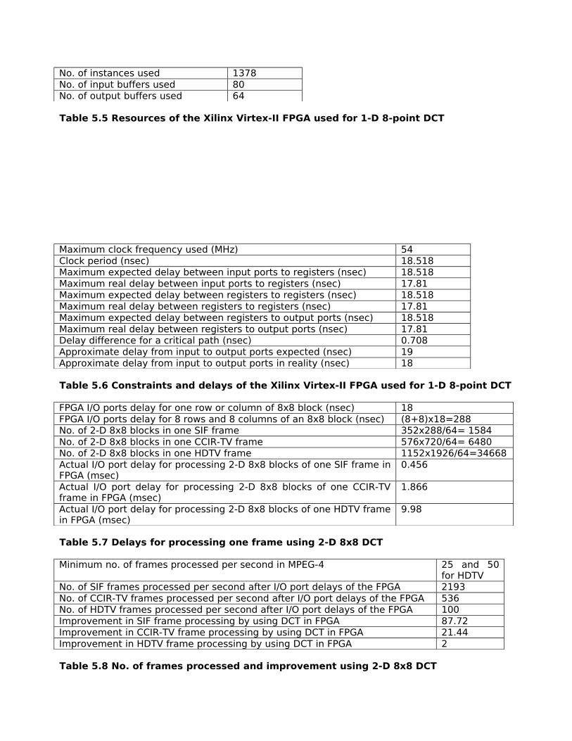
No. of instances used 1378No. of input buffers used 80No. of output buffers used 64

Table 5.5 Resources of the Xilinx Virtex-II FPGA used for 1-D 8-point DCT

Maximum clock frequency used (MHz) 54Clock period (nsec) 18.518Maximum expected delay between input ports to registers (nsec) 18.518Maximum real delay between input ports to registers (nsec) 17.81Maximum expected delay between registers to registers (nsec) 18.518Maximum real delay between registers to registers (nsec) 17.81Maximum expected delay between registers to output ports (nsec) 18.518Maximum real delay between registers to output ports (nsec) 17.81Delay difference for a critical path (nsec) 0.708Approximate delay from input to output ports expected (nsec) 19Approximate delay from input to output ports in reality (nsec) 18

Table 5.6 Constraints and delays of the Xilinx Virtex-II FPGA used for 1-D 8-point DCT

FPGA I/O ports delay for one row or column of 8x8 block (nsec) 18FPGA I/O ports delay for 8 rows and 8 columns of an 8x8 block (nsec) (8+8)x18=288No. of 2-D 8x8 blocks in one SIF frame 352x288/64= 1584No. of 2-D 8x8 blocks in one CCIR-TV frame 576x720/64= 6480No. of 2-D 8x8 blocks in one HDTV frame 1152x1926/64=34668Actual I/O port delay for processing 2-D 8x8 blocks of one SIF frame in FPGA (msec)

0.456

Actual I/O port delay for processing 2-D 8x8 blocks of one CCIR-TV frame in FPGA (msec)

1.866

Actual I/O port delay for processing 2-D 8x8 blocks of one HDTV frame in FPGA (msec)

9.98

Table 5.7 Delays for processing one frame using 2-D 8x8 DCT

Minimum no. of frames processed per second in MPEG-4 25 and 50 for HDTV

No. of SIF frames processed per second after I/O port delays of the FPGA 2193No. of CCIR-TV frames processed per second after I/O port delays of the FPGA 536No. of HDTV frames processed per second after I/O port delays of the FPGA 100Improvement in SIF frame processing by using DCT in FPGA 87.72Improvement in CCIR-TV frame processing by using DCT in FPGA 21.44Improvement in HDTV frame processing by using DCT in FPGA 2

Table 5.8 No. of frames processed and improvement using 2-D 8x8 DCT

5.4 Altera’s FPGA Implementation

We now implement the 8-point DCT/IDCT algorithm is Altera’s Acex-1K FPGA. This family is chosen due to good timing parameters, i.e., less I/O ports delays than other Altera FPGA series. We have selected the Acex-1K EP1K50F256 FPGA having a maximum speed grade of –3. The clock frequency used in this case is far less than the one used for Xilinx’s FPGA. This means less numbers of video frames can be processed per second by 2-D 8x8 DCT/IDCT in Altera than Xilinx.

The details of the DCT/IDCT implementation for Altera’s FPGA are mentioned in Tables 5.9(a) till 5.16. The calculations done for I/O port delays are similar to the ones done before.

Device used EP1K50F256

Speed grade of the FPGA used -3I/O ports available 186I/O ports used 144Logic cells available 2880Logic cells used 1482Carrys available 2880Carry used 1206DFF available 2880DFF used 0No. of carrys used 1206No. of nets used 2260No. of instances used 2580

Table 5.9 Resources of the Altera Acex-1K FPGA used for 1-D 8-point IDCT

Maximum clock frequency used (MHz) 16Clock period (nsec) 62.50Maximum expected delay between input ports to registers (nsec) 62.50Maximum real delay between input ports to registers (nsec) 60.65Maximum expected delay between registers to registers (nsec) 62.50Maximum real delay between registers to registers (nsec) 60.65Maximum expected delay between registers to output ports (nsec) 62.50Maximum real delay between registers to output ports (nsec) 60.65Delay difference for a critical path (nsec) 1.85Approximate delay from input to output ports expected (nsec) 63Approximate delay from input to output ports in reality (nsec) 61

Table 5.10 Constraints and delays of the Altera Acex-1K FPGA used for 1-D 8-point IDCT

FPGA I/O ports delay for one row or column of 8x8 block (nsec) 61FPGA I/O ports delay for 8 rows and 8 columns of an 8x8 block (sec) (8+8)x61= 0.976No. of 2-D 8x8 blocks in one SIF frame 352x288/64= 1584No. of 2-D 8x8 blocks in one CCIR-TV frame 576x720/64= 6480No. of 2-D 8x8 blocks in one HDTV frame 1152x1926/64=34668Actual I/O port delay for processing 2-D 8x8 blocks of one SIF frame in FPGA (msec)

1.545

Actual I/O port delay for processing 2-D 8x8 blocks of one CCIR-TV frame in FPGA (msec)

6.324

Actual I/O port delay for processing 2-D 8x8 blocks of one HDTV frame in FPGA (msec)

33.836

Table 5.11 Delays in processing one frame using 2-D 8x8 IDCT

Minimum no. of frames processed per second in MPEG-4 25 and 50 for HDTV

No. of SIF frames processed per second after I/O port delays of the FPGA 647No. of CCIR-TV frames processed per second after I/O port delays of the FPGA 158No. of HDTV frames processed per second after I/O port delays of the FPGA 29Improvement in SIF frame processing by using IDCT in FPGA 25.88Improvement in CCIR-TV frame processing by using IDCT in FPGA 6.32Improvement in HDTV frame processing by using IDCT in FPGA 0.58

Table 5.12 No. of frames processed and improvement using 2-D 8x8 IDCT on FPGA

Device used EP1K50F256

Speed grade of the FPGA used -3I/O ports available 186I/O ports used 144Logic cells available 2880Logic cells used 1303Carrys available 2880Carry used 1053DFF available 2880DFF used 0No. of carrys used 1206No. of nets used 2660No. of instances used 2580

Table 5.13 Resources of the Altera Acex-1K FPGA used for 1-D 8-point DCT

Maximum clock frequency used (MHz) 16Clock period (nsec) 62.50Maximum expected delay between input ports to registers (nsec) 62.50Maximum real delay between input ports to registers (nsec) 60.65Maximum expected delay between registers to registers (nsec) 62.50Maximum real delay between registers to registers (nsec) 60.65Maximum expected delay between registers to output ports (nsec) 62.50Maximum real delay between registers to output ports (nsec) 60.65Delay difference for a critical path (nsec) 1.85Approximate delay from input to output ports expected (nsec) 63Approximate delay from input to output ports in reality (nsec) 61

Table 5.14 Constraints and delays of the Altera Acex-1K FPGA used for 1-D 8-point DCT

FPGA I/O ports delay for one row or column of 8x8 block (nsec) 61FPGA I/O ports delay for 8 rows and 8 columns of an 8x8 block (sec) (8+8)x61= 0.976No. of 2-D 8x8 blocks in one SIF frame 352x288/64= 1584No. of 2-D 8x8 blocks in one CCIR-TV frame 576x720/64= 6480No. of 2-D 8x8 blocks in one HDTV frame 1152x1926/64=34668Actual I/O port delay for processing 2-D 8x8 blocks of one SIF frame in FPGA (msec)

1.545

Actual I/O port delay for processing 2-D 8x8 blocks of one CCIR-TV frame in FPGA (msec)

6.324

Actual I/O port delay for processing 2-D 8x8 blocks of one HDTV frame in FPGA (msec)

33.836

Table 5.15 Delays in one frame processing using 2-D 8x8 DCT

Minimum no. of frames processed per second in MPEG-4 25 and 50 for HDTV

No. of SIF frames processed per second after I/O port delays of the FPGA 647No. of CCIR-TV frames processed per second after I/O port delays of the FPGA 158No. of HDTV frames processed per second after I/O port delays of the FPGA 29Improvement in SIF frame processing by using DCT in FPGA 25.88Improvement in CCIR-TV frame processing by using DCT in FPGA 6.32Improvement in HDTV frame processing by using DCT in FPGA 0.58

Table 5.16 No. of frames processed and improvement using 2-D 8x8 DCT

5.5 Lucent’s FPGA Implementation

The last FPGA technology selected for the implementation of 8-point DCT/IDCT algorithm is Lucent’s ORCA-3C/3T series. We have selected the ORCA-3C/3T OR3T30B256 FPGA having a maximum speed grade of 7. The clock frequency used in this case is higher than Altera but less than the one used for Xilinx’s FPGA. This means number of video frames processed per second by 2-D 8x8 DCT/IDCT in Lucent’s FPGA is higher than Altera but less than Xilinx. The details of the DCT/IDCT implementation for Lucent’s FPGA are mentioned in Tables 5.17(a) till 5.24.

Device used OR3T30B256

Speed grade of the FPGA used 7

I/O ports available 223

I/O ports used 144

Look up tables available 1568Look up tables used 1488PFUs available 196PFUs used 186Flip flops available 1568Flip flops used 0No. of nets used 1784

No. of instances used 520No. of input buffers (IBM) used 80No. of output buffers (ob6) used 64

Table 5.17 Resources of the Lucent ORCA-3C/3T FPGA used for 1-D 8-point IDCT

Maximum clock frequency used (MHz) 22Clock period (nsec) 45.45Maximum expected delay between input ports to registers (nsec) 45.45Maximum real delay between input ports to registers (nsec) 45.08Maximum expected delay between registers to registers (nsec) 45.45Maximum real delay between registers to registers (nsec) 45.08Maximum expected delay between registers to output ports (nsec) 45.45Maximum real delay between registers to output ports (nsec) 45.08Delay difference of a critical path (nsec) 0.37Approximate delay from input to output ports expected (nsec) 46Approximate delay from input to output ports in reality (nsec) 45

Table 5.18 Constraints and delays of the ORCA-3C/3T FPGA used for 1-D 8-point IDCT

FPGA I/O ports delay for one row or column of 8x8 block (nsec) 45FPGA I/O ports delay for 8 rows and 8 columns of an 8x8 block (sec) (8+8)x45= 0.72No. of 2-D 8x8 blocks in one SIF frame 352x288/64= 1584No. of 2-D 8x8 blocks in one CCIR-TV frame 576x720/64= 6480No. of 2-D 8x8 blocks in one HDTV frame 1152x1926/64=34668Actual I/O port delay for processing 2-D 8x8 blocks of one SIF frame in FPGA (msec)

1.140

Actual I/O port delay for processing 2-D 8x8 blocks of one CCIR-TV frame in FPGA (msec)

4.666

Actual I/O port delay for processing 2-D 8x8 blocks of one HDTV frame in FPGA (msec)

24.961

Table 5.19 Delays in processing one frame using 2-D 8X8 IDCT

Minimum no. of frames processed per second in MPEG-4 25 and 50 for HDTV

No. of SIF frames processed per second after I/O port delays of the FPGA 877No. of CCIR-TV frames processed per second after I/O port delays of the FPGA 214No. of HDTV frames processed per second after I/O port delays of the FPGA 40Improvement in SIF frame processing by using IDCT in FPGA 35.08Improvement in CCIR-TV frame processing by using IDCT in FPGA 8.56Improvement in HDTV frame processing by using IDCT in FPGA 0.80

Table 5.20 No. of frames processed and speed up using 2-D 8X8 IDCT

Device used OR3T30B256

Speed grade of the FPGA used 7

I/O ports available 223

I/O ports used 144

Look up tables available 1568Look up tables used 1320PFUs available 196PFUs used 165Flip flops available 1568Flip flops used 0No. of nets used 1784No. of instances used 520No. of input buffers (IBM) used 80No. of output buffers (ob6) used 64

Table 5.21 Resources of the Lucent ORCA-3C/3T FPGA used for 1-D 8-point DCT

Maximum clock frequency used (MHz) 22Clock period (nsec) 45.45Maximum expected delay between input ports to registers (nsec) 45.45Maximum real delay between input ports to registers (nsec) 43.64Maximum expected delay between registers to registers (nsec) 45.45Maximum real delay between registers to registers (nsec) 43.64Maximum expected delay between registers to output ports (nsec) 45.45Maximum real delay between registers to output ports (nsec) 43.64Delay difference of a critical path (nsec) 1.82Approximate delay from input to output ports expected (nsec) 46Approximate delay from input to output ports in reality (nsec) 44

Table 5.22 Constraints and delays of the ORCA-3C/3T FPGA used for 1-D 8-point DCT

FPGA I/O ports delay for one row or column of 8x8 block (nsec) 44FPGA I/O ports delay for 8 rows and 8 columns of an 8x8 block (sec) (8+8)x44= 0.704No. of 2-D 8x8 blocks in one SIF frame 352x288/64= 1584No. of 2-D 8x8 blocks in one CCIR-TV frame 576x720/64= 6480No. of 2-D 8x8 blocks in one HDTV frame 1152x1926/64=34668Actual I/O port delay for processing 2-D 8x8 blocks of one SIF frame in FPGA (msec)

1.115

Actual I/O port delay for processing 2-D 8x8 blocks of one CCIR-TV frame in FPGA (msec)

4.562

Actual I/O port delay for processing 2-D 8x8 blocks of one HDTV frame in FPGA (msec)

24.406

Table 5.23 Delays in processing one frame using 2-D 8x8 DCT

Minimum no. of frames processed per second in MPEG-4 25 and 50 for HDTV

No. of SIF frames processed per second after I/O port delays of the FPGA 896No. of CCIR-TV frames processed per second after I/O port delays of the FPGA 219No. of HDTV frames processed per second after I/O port delays of the FPGA 40Improvement in SIF frame processing by using DCT in FPGA 35.84Improvement in CCIR-TV frame processing by using DCT in FPGA 8.76Improvement in HDTV frame processing by using DCT in FPGA 0.80

Table 5.24 No. of frames processed and speed up using 2-D 8x8 DCT

5.6 Overall Results

We present the synthesis results in bar graphs so that one can easily compare the performances of different FPGA technologies implementing DCT/IDCT.

FPGA Technology vs. Clock Frequency Used

0

10

20

30

40

50

60

Xilinx Lucent Altera

FPGA Technology

Clo

ck F

req

uen

cy

(MH

z)

Figure 5.8 Comparing different FPGA technologies with the clock frequencies used to implement 1-D 8-point DCT

FPGA Technology vs. Clock Frequeny Used

0

10

20

30

40

50

60

70

Xilinx Lucent Altera

FPGA Technology

Clo

ck F

req

uen

cy

(MH

z)

Figure 5.9 Comparing different FPGA technologies with the clock frequencies used to implement 1-D 8-point IDCT

The results in Figures 5.8 and 5.9 indicate that highest clock frequency is used for 2-D 8X8 DCT/IDCT implementation using Xilinx’s FPGA. This means Xilinx’s FPGA provides the least I/O port delay and maximum speed up or improvement in video frame processing than the other two FPGA technologies.

FPGA technology vs. SIF frame processing per second

0500

1000150020002500

Xilinx Lucent Altera

FPGA technology

SIF

fra

me

pro

cess

ing

per

se

con

d

Figure 5.10 Comparing different FPGA technologies to SIF frames processed per second using 2-D 8x8 DCT

FPGA technology vs. SIF frame processing per second

0

1000

2000

3000

Xilinx Lucent Altera

FPGA technology

SIF

fra

me

pro

cess

ing

per

s

eco

nd

Figure 5.11 Comparing different FPGA technologies to SIF frames processed per second using 2-D 8x8 IDCT

It can be seen from Figures 5.10 and 5.11 that Xilinx’s FPGA processes the highest number of SIF frames per second then other FPGA. The other two FPGA are also processing frames higher than the minimum required rates. In fact our implementation of DCT/IDCT in hardware shows high SIF frame processing rates especially in case of using Xilinx’s FPGA.

FPGA technology vs. CCIR-TV frames processed per second

0

200

400

600

Xilinx Lucent Altera

FPGA technology

CC

IR-T

V f

ram

es

pro

cess

ed p

er

seco

nd

Figure 5.12 Comparing different FPGA technologies to CCIR-TV frames processed per second using 2-D 8x8 DCT

FPGA technology vs. CCIR-TV frames processed per second

0

200

400

600

800

Xilinx Lucent Altera

FPGA technology

CC

IR-T

V f

ram

es

pro

cess

ed p

er

seco

nd

Figure 5.13 Comparing different FPGA technologies to CCIR-TV frames processed per second using 2-D 8x8 IDCT

From Figures 5.12 and 5.13, it is evident number of CCIR-TV frames processed per second by Xilinx’s FPGA are much higher. The other two FPGA are also processing frames higher than the minimum required rates. Hence, our implementation of a fast DCT/IDCT shows the advantage in terms of higher frame processing rates.

FPGA technology vs. HDTV frames processed per second

0

50

100

150

Xilinx Lucent Altera

FPGA technology

HD

TV

fra

mes

p

roce

ssed

per

se

con

d

Figure 5.14 Comparing different FPGA technologies to HDTV frames processed per second using 2-D 8x8 DCT

FPGA technology vs. HDTV frame processed per second

0

50

100

150

Xilinx Lucent Altera

FPGA technology

HD

TV

fra

me

pro

cess

ing

rat

es

pe

r se

con

d

Figure 5.15 Comparing different FPGA technologies to HDTV frames processed per second using 2-D 8x8 IDCT

Finally, Figures 5.14 and 5.15 depict that only Xilinx’s FPGA is able to process twice the rate required by HDTV, which is a remarkable achievement. The other two FPGA are processing frames less than the minimum requirement. It must be mentioned that the author has found no other existing DCT based FPGA implementations, which can process HDTV video frames equal or higher than the minimum required rate. By implementing a very fast DCT algorithm in Xilinx’s FPGA, the author has overcome this problem to provide the much needed improvement for processing HDTV frames at a higher rate.

5.7 Conclusions

Looking carefully at the synthesis results, we can see high SIF and CCIR-TV frame processing rates by the stand-alone FPGA units. These results show that we have used 54 MHz and 60 MHz for the Xilinx FPGA chip to implement 8-point DCT/IDCT. The video frame processing rates achieved for 2-D 8x8 DCT (according to MPEG-4 standard), are 2193 SIF, 536 CCIR-TV and 100 HDTV frames. For 8x8 2-D IDCT these rates have changed to 2469 SIF, 600 CCIR-TV and 112 HDTV frames, respectively.

For Altera’s FPGA, clock frequency of 16 MHz has been used to implement 8-point DCT/IDCT. The video frame processing rates achieved (according to MPEG-4 standard), are 647 SIF, 158 CCIR-TV and 29 HDTV frames. In case of Lucent’s FPGA, clock frequency of 22 MHz has been used to implement 8-point DCT/IDCT. The video frame processing rates achieved for 2-D 8x8 DCT (according to MPEG-4 standard), are 896 SIF, 219 CCIR-TV and 40 HDTV frames. For 2-D 8x8 IDCT these rates have changed to 877 SIF, 214 CCIR-TV and 40 HDTV frames, respectively.

It should be clear that for other frame formats such as QCIF the frame processing rates would be much higher. The results mentioned above, show the advantage of implementing DCT and IDCT in hardware using FPGA to speed up video processing. In particular, Xilinx’s FPGA is even able to process HDTV frames twice the minimum required rate.

Chapter 6

Conclusion and Future Work

6.1 Conclusion

In this thesis, we have made a comprehensive comparison between data compression transforms particularly the discrete cosine transform (DCT) and the discrete wavelet transform (DWT). The comparison is based upon their performance for multimedia applications, e.g., still images and motion video. To gain insight into the effectiveness of these transforms for still image compression, we generated results using VcDemo [5] software. Thus results proved the excellent compression performance provided by DWT based algorithms in terms of visual quality and higher PSNR.

The performance of DCT and DWT was discussed based upon PSNR results for images and motion video, response to human visual system (HVS), and the complexities in implementation. For still image compression, DWT based coders have outperformed DCT coders both in terms of image quality and higher PSNR. For motion video, the performance of some DWT-based coders like ZTE (mentioned in Chapters 2 and 4) is near or equivalent to that of DCT- based coders. Motion-compensation is still the biggest issue for designers to implement it with less complexity and greater improvement in DWT-based coders. In terms of complexities involved in implementing DCT and DWT in both fixed and reconfigurable hardware units, DCT achieves the fastest computational performance due to fast algorithms.

This thesis also described the implementation of an 8x8 DCT and inverse DCT for different FPGA technologies using Modified Loeffler Algorithm [14][15]. For different frame formats, all the stand-alone FPGA units were able to provide processing rates higher than the minimum rates. In particular, Xilinx’s FPGA was even able to process HDTV frames at twice the required rate. These results indicate the main advantages of DCT implementation to provide the required video processing performance.

6.2 Future Work

Most of the DCT and DWT based compression algorithms have been implemented in software using high-level languages such as C or Java. Such an approach provides maximum flexibility but lacks performance. At the same time, proprietary hardware implementations in ASIC were proposed to speed up such compression algorithms. But this is an inflexible solution and lacks cost efficiency.

A new approach is the combination of programmable processors with reconfigurable hardware units. Non-time critical operations are implemented in software (providing flexibility) while time -critical operations such as DCT or DWT, are implemented in hardware using FPGA (providing speed up). We must note that the performance of FPGAs is quickly nearing that of ASICS. Therefore, our DCT implementation also targeted different FPGA technologies. In the mentioned approach, reconfigurable hardware is augmented like a functional unit, commonly referred to as a reconfigurable unit. As future work, we would like to propose the possible integration of our FPGA design in such processors. In particular we also propose the integration of our design in the MOLEN processor [16], which utilize microcode to control both the reconfiguration and execution process of the reconfigurable unit. Additionally, research is being carried out to further reduce the I/O ports delay of FPGA to speed up computation.

References[1] J. Shapiro, “Embedded image coding using zerotrees of wavelet coefficients,” IEEE Trans. Signal Processing, vol. 41, pp. 3445-3462, Dec 1993.

[2] Said, A. and Pearlman, “A new fast and efficient image codec based on set partitioning in hierarchical trees,” IEEE Trans. on Circuits and Systems for Video Technology, Vol. 6, No.3, pp. 243-250, 1996.[3] S.A. Matrucci and I. Sodagar, “A zerotree wavelet video coder,” IEEE Trans. on Circuits and Systems for Video Technology, Vol. 7, No.1, pp. 109-118, Feb.1997.[4] A. Skodras and T. Ebrahimi, “ The JPEG 2000 still image compression standard,” IEEE Signal Processing Magazine, Sep. 2001.[5] Information and Communication Theory Group, VcDemo: Image and video compression learning tool. TU Delft. Available;http://www-ict.its.tudelft.nl/~inald/vcdemo[6] Video Compression, Available: http://www.dspworx.com/primer_video_compression.htm[7] R. Queiroz and K.R. Rao, “Wavelet transform in a JPEG-like image coder,” IEEE Trans. on Circuits and Systems for Video Technology, Vol. 7, No.2, pp. 419-424, April 1997.[8] D. Santa-Cruz and T. Ebrahimi, “ A study of JPEG 2000 still image coding versus other standards,” In Proc. of the 10th European Signal Processing Conference, Vol. 2, PP. 673-676, Finland, Sep. 5-8, 2000.[9] S. Saha, Image compression - from DCT to Wavelets: A Review, Available:http://www.acm.org/crossroads/xrds6-3/sahaimgcoding.html#Fig6[10] JPEG vs. JPEG 2000- Comparison, Available: http://www.dspworx.com/primer_jpeg_vs__jpeg2000.htm[11] Visio wave dynamic coding white paper, NEC research index, Available: http://citeseer.nj.nec.com/cs[12] Wim Sweldens, Wavelets and the lifting scheme: A 5 minute tour, NEC research index, Available: http://citeseer.nj.nec.com/cs[13] Amphion’s FPGAs and ASICs, Available: http://www.amphion.com/video.html[14] C. Loeffler and A. Lightenberg, “Practical fast 1-D DCT algorithms with 11 Multiplications,” Proceedings of the International Conference on Acoustics, Speech and Signal Processing (ICASSP ’89), Scotland, May 1989, pp. 988-991.[15] M. Sima, S. Cotafona, S. Vassiliadis and J.T.J. van Eindhoven, “ 8x8 IDCT Implementation on an FPGA-augmented Trimedia,” IEEE Symposium on FPGAs for Custom Computing Machines (FCCM 2001), California, April 2001.[16] S. Cotafona, S. Vassiliadis and S. Wong, “The MOLEN rm-processor,” 11th International Conference on Field Programmable Logic and Applications (FLP), 2001.

Appendix A

Description of Source Files

VHDL Simulation Files

We have made two simulation files each for running 8-point 1-D DCT and IDCT algorithm in the environment of ModelSimTM software.

The names of these files are:

DCTsim1_1.vhd

IDCTsim1_1.vhd

Each file could be run independently and contains necessary details of the entities, architectures and the test bench written specially to simulate the VHDL code. It should be mentioned that while running any of these files, there wouldn’t be any need of additional VHDL files. The entities are well defined and given names according to the algorithm. Special scaling multipliers have been used in both DCT and IDCT VHDL source files so that the outputs of one file could be used as inputs to other. The final results after DCT and IDCT are almost same as the original. The algorithm has been implemented using fixed-point arithmetic instead of floating–point to reduce the cost of computation.

VHDL Synthesis Files

We have made two synthesis files each for running 8-point 1-D DCT and IDCT algorithm in the environment of Leonardo-SpectrumTM software.

The names of these files are:

DCTsim1_1.vhd

IDCTsim1_1.vhd

Although the names are the same but both of these files do not contain any test bench as in case of simulation. The names of these files could be changed or they should be kept in a separate directory so that there is no conflict of names with the simulation files, as done by the author himself. Each file could be synthesized for different FPGAs such as Xilinx, Altera, Atmel and Lucent.

Post Script Source File

An electronic version of the thesis is also submitted so that it can be used as reference. The name of the files is:

Msc_thesis_kh.ps