visual dictionary learning for joint object -

Visual Dictionary Learning for Joint Object

Categorization and Segmentation

Aastha Jain, Luca Zappella, Patrick McClure, and Rene Vidal

Center for Imaging Science, Johns Hopkins University

Abstract. Representing objects using elements from a visual dictio-nary is widely used in object detection and categorization. Prior workon dictionary learning has shown improvements in the accuracy of ob-ject detection and categorization by learning discriminative dictionaries.However none of these dictionaries are learnt for joint object categoriza-tion and segmentation. Moreover, dictionary learning is often done sep-arately from classifier training, which reduces the discriminative powerof the model. In this paper, we formulate the semantic segmentationproblem as a joint categorization, segmentation and dictionary learn-ing problem. To that end, we propose a latent conditional random field(CRF) model in which the observed variables are pixel category labelsand the latent variables are visual word assignments. The CRF energyconsists of a bottom-up segmentation cost, a top-down bag of (latent)words categorization cost, and a dictionary learning cost. Together, thesecosts capture relationships between image features and visual words, re-lationships between visual words and object categories, and spatial re-lationships among visual words. The segmentation, categorization, anddictionary learning parameters are learnt jointly using latent structuralSVMs, and the segmentation and visual words assignments are inferredjointly using energy minimization techniques. Experiments on the Graz02and CamVid datasets demonstrate the performance of our approach.

1 Introduction

Joint categorization and segmentation (JCaS) refers to the problem of assigningan object category label to each pixel in a given image. Most existing solutionsto this problem use conditional random field (CRF) formulations. The sites ofthe CRF are image pixels [1], patches [2, 3], superpixels [4–7], or a hierarchy ofregions [8, 9]. Local interactions among these sites are captured by unary andpairwise potentials, which model, respectively, the cost of assigning a categorylabel to each site and the spatial smoothness of the segmentation. Long-rangeinteractions among many sites of the CRF are captured by higher-order poten-tials, which model the statistics of an object and/or encode contextual informa-tion. However, such long-range interactions are typically restricted to fairly localneighborhoods to avoid crossing the boundaries of an object. Notable exceptionsare [10], which uses interactions among several sites to model co-occurrencestatistics between object categories, and [11, 12], which use a bag-of-features(BoF) model to define a potential over the whole region occupied by the object.

A. Fitzgibbon et al. (Eds.): ECCV 2012, Part V, LNCS 7576, pp. 718–731, 2012.c© Springer-Verlag Berlin Heidelberg 2012

Visual Dictionary Learning for Joint Object Categorization and Segmentation 719

The BoF approach is one of the most widely used models for object catego-rization. In this approach, an object is represented by the distribution of a setof visual words, which are usually obtained by K-means clustering of a set offeature descriptors obtained from the training images. While BoF methods haveshown good performance in object categorization [13–15], the visual dictionarymay not be descriptive of the object categories, because the words are learnt inan unsupervised manner. Discriminative dictionary learning methods for objectcategorization such as [16] incorporate class-specific information during dictio-nary learning, which improves the discriminative capability of the dictionary.However, one drawback of this technique is that the dictionary learning andclassifier training steps are done separately. This leads to reduced categorizationaccuracy because the words, while individually discriminative, may not be opti-mal for categorization. The work of [17] overcomes this drawback by learning thedictionary and the classifiers simultaneously, and shows improved performance.

In our view, the method used for learning the dictionary depends heavily onthe task at hand. To the best of our knowledge, none of the existing dictionarylearning techniques has been used to learn dictionaries that are specifically de-signed for the JCaS problem. For instance, the work of [18] combines CRFs withdictionary learning for object detection purposes, but it does not address seg-mentation or categorization. Also, the work of [12] uses dictionaries to constructthe higher-order CRF potentials, but the method for learning the dictionary isunsupervisedK-means. Moreover, this dictionary is kept fixed while learning thecategorization and segmentation parameters of the CRF. We believe that unsu-pervised, discriminative or object-specific dictionaries are suboptimal for solvingthe JCaS problem, because they are learnt independently from the categoriza-tion and segmentation parameters of the CRF, and hence their discriminativepower is compromised.

In this work we propose a JCaS framework in which the visual dictionary islearnt jointly with the CRF categorization and segmentation parameters. In ourframework, the assignment of key-points to visual words is assumed to be un-known and is modeled as a latent variable of the CRF, which needs to be inferredduring inference and training. In addition to the standard potentials defined toensure smoothness of the segmentation, we introduce a set of potentials thatmodel the interaction between feature descriptors and visual word assignments,and another set of potentials that model the probability that each visual wordbelongs to a particular object category. We also extend this framework beyondthe BoF model and introduce additional potentials that take into account inter-actions between the visual word assignments of neighboring key-points.

We show that the parameters of this model can be learnt jointly using latentstructural SVMs. The visual dictionary learnt in this manner uses the informa-tion from the categorization and segmentation parameters, which increases thediscriminative power of our model. Given the model parameters, we show thatthe segmentation and visual word assignments can be found using graph cutsor loopy-belief propagation. Experiments on the Graz02 and CamVid databasesshow that our approach improves segmentation accuracy of structured objects.

720 A. Jain et al.

2 A CRF-BoF Model for JCaS

In this section, we review the CRF model for JCaS proposed in [12], which isbased on a BoF categorization cost. While [12] uses kernel SVM classifiers withthe intersection kernel, we will describe the model using linear classifiers.

CRF Structure. The CRF is defined over a set of superpixels V extractedfrom the image I. Each site i ∈ V is associated with an object category labelxi ∈ L = {1, . . . , L}. The labelling of the image is denoted by the vector x ∈ L|V|.The interaction between various sites of the CRF is captured by the set of edgesE ⊂ V ×V , where each edge eij ∈ E corresponds to a pair of superpixels i, j ∈ Vthat share a boundary. Besides sites and edges, we can also define higher-ordercliques. A clique is a subset of sites c ⊂ V whose labels, xc, are conditionallydependent on each other. For example, a site i ∈ V is a clique of size 1 and anedge eij ∈ E corresponds to a clique of size 2.

Having defined the structure of the random field, in what follows we definethe CRF energy, which consists of a segmentation cost and a categorization cost.

Bottom-Up Segmentation Cost. We define the segmentation cost as:

Eseg(x, I) = λU∑

i∈VψUi (xi, I) + λP

∑

eij∈EψPij(xi, xj , I) = w�

segΨseg(x, I), (1)

where λU ≥ 0 and λP ≥ 0 are the relative weights of the unary and pairwise

potentials, w�seg =

[λU λP

]and Ψseg(x, I) =

[ ∑i∈V ψ

Ui (xi, I)∑

eij∈E ψPij(xi, xj , I)

].

The unary potential, ψUi (xi, I), models the cost of assigning a class label xi ∈

L to superpixel i in image I. It is defined as the score of a kernel SVM classifier forclass xi applied to a normalized histogram of quantized SIFT features extractedfrom a neighborhood of superpixel i of size τ (see [19]). The classifier for classl ∈ L is trained using the normalized histograms extracted from the superpixelsin the training set whose label is l. We use the RBF-χ2 kernel k(f, g) = e−γχ2(f,g).

The pairwise potential, ψPij(xi, xj , I), models the cost of assigning labels xi and

xj to sites i and j, respectively. When using a CRF formulation for segmentation,the pairwise potentials are typically used to ensure the smoothness of the label

assignments. We use a contrast sensitive costLijδ(xi �=xj)

1+‖Ii−Ij‖ , where Lij is the length

of the shared boundary between superpixels i and j, and Ii and Ij are the meancolor (in the LUV space) of superpixels i and j, respectively.

BoF Categorization Cost. The segmentation cost models only the local fea-tures and characteristics of the image. To infer the class of an object, we alsoneed to account for long-range interactions between various sites in the CRF.

One way to capture such long-range interactions is to represent each objectclass with a BoF model, and define a categorization potential over all the sitescorresponding to an object class. To that end, let {θk}k∈K be a dictionary of|K| visual words. This dictionary is obtained by applying K-means to the SIFTfeatures extracted from all the superpixels in the training images. We represent


each image I with |L| histograms of these visual words. More specifically, let SI

denote a set of key-points extracted from image I and let dIp denote the feature

descriptor of key-point p ∈ SI . Each descriptor dIp is assigned to its closest word,

θ(dIp), and a histogram of these words, hl(x, I) ∈ RK+ , is used to represent the

portion of the image occupied by object class l. We can write the histogram bincount for class l corresponding to visual word k as

hl,k(x, I) =∑

p∈SI

δ(θ(dIp) = θk)δ(xip = l) =∑

p∈SkI

δ(xip = l), (2)

where ip ∈ V is the superpixel associated with key-point p ∈ SI and SkI ⊂ SI is

the set of key-points associated to word k.

Let us now define a classifier Φl for each class label l, where Φl(h) : R|K|+ �→ R

represents the score assigned to the histogram h. Using a linear classifier we have

Φl(h) = α�l h+ βl =

∑

k∈Kαl,khk + βl, (3)

where αl ∈ R|K| and βl ∈ R are the parameters of the linear classifier for class

l. With the above notation, we define a categorization cost, Ecat, as the sum ofthe categorization costs for each class, i.e.,

Ecat(x, I) =∑

l∈LΦl(hl(x, I))δ(||hl(x, I)|| > 0). (4)

Notice that we pay no cost when no key-point is assigned to category l, i.e.,Ecat(x, I) = 0 when hl(x, I) = 0. Also, since we wish to minimize this cost, wetrain classifiers Φl to assign low scores to histograms in class l and high scoresto histograms corresponding to other classes (contrary to the usual convention).

Although the energy Ecat may seem a complicated function of x, notice thatwe can write it linearly in terms of the classifier parameters as

Ecat(x, I) = w�catΨcat(x, I) =

[ · · · αl,k βl · · ·]

⎡

⎢⎢⎢⎢⎣

...ψHl,k(x, I)

ψδl (x, I)...

⎤

⎥⎥⎥⎥⎦, (5)

where ψHl,k(x, I) =

∑p∈Sk

Iδ(xip = l) and ψδ

l (x, I) = min{1,∑p∈SIδ(xip = l)}.

Inference and Learning. The inference task is to minimize the segmentationand categorization cost :

Eseg+cat(x, I) = w�seg+catΨseg+cat(x, I) =

[w�

seg w�cat

] [Ψseg(x, I)Ψcat(x, I)

]. (6)

The segmentation cost is a standard unary+pairwise cost that can be minimizedby graph cuts [20]. On the other hand, the categorization cost is a higher-ordercost defined over a clique of size |SI | formed by the all the superpixels thatcontain key-points. It is shown in [12] that this higher-order potential belongsto the class of robust Potts model [21], which can be minimized by graph cuts.

722 A. Jain et al.

The learning task is to estimate the parameters of the energy wseg+cat froma training set of segmented images {Ij}Nj=1 and their corresponding labellings

{xj}Nj=1. Since the energy is linear in the parameters λU , λP , {αl, βl}l∈L, we canuse the cutting plane training algorithm for structural SVMs [22] to learn theseparameters, as shown in [12]. Since negative examples (wrong segmentations) arenot given, at each step of the cutting plane algorithm, the wrong segmentationwith the worst margin is selected. This can also be done using graph cuts.

For more details on inference and learning, we refer the reader to [12].

3 A Latent CRF-BoF Model for JCaS

In the BoF model for JCaS described in the previous section, K-means cluster-ing is used to generate the visual dictionary. Therefore, this visual dictionaryis learnt independently from the categorization and segmentation parameters.Since dictionary learning helps categorization and segmentation, and knowledgeabout the categorization and segmentation parameters helps dictionary learn-ing, a more meaningful dictionary could be obtained by learning the visual wordstogether with the categorization and segmentation parameters.

In this section, we will re-formulate the energy E to incorporate the visualwords as additional parameters of the energy and the visual word assignmentsas latent variables. We introduce a categorization cost that depends on both thesegmentation and the visual word assignments. This cost captures the relation-ships among the visual words and the object categories. We also introduce a newdictionary learning cost, which relates the image features to the visual words.

Latent BoF Categorization Cost. Let {θk}k∈K be an (unknown) dictionaryof |K| visual words. Instead of fixing the visual word assignment prior to cate-gorization, we associate a random variable zp ∈ K with every key-point p ∈ SI .The vector z ∈ K|SI | is then a latent variable of a CRF defined over the key-points. Let us recall the categorization cost introduced in (4)-(5). This costdepends on the histogram counts hl,k(x, I) =

∑p∈Sk

Iδ(xip = l), where the set

of key-points SI is divided into |K| disjoint subsets SkI containing the key-points

assigned to visual word k. Since the word assignments are unknown, so are thesets Sk

I . Nonetheless, we can easily express hl,k in terms of the word assignmentvariables as

hl,k(x, z, I) =∑

p∈SI

δ(xip = l, zp = k). (7)

Therefore, the categorization cost in (5) can be re-written as:

Ecat(x, z, I) = w�catΨcat(x, z, I) =

[ · · · αl,k βl · · ·]

⎡

⎢⎢⎢⎢⎣

...ψHl,k(x, z, I)

ψδl (x, I)...

⎤

⎥⎥⎥⎥⎦, (8)

where ψHl,k(x, z, I) =

∑p∈SI

δ(xip = l, zp = k).


Dictionary Learning Cost. We now define a dictionary learning cost thatrelates the word assignments {z}p∈SI to the image features {dIp}p∈SI . In standard

K-means, the assignment of a feature dIp to a visual word θk is given by

zp = argmink∈K

||θk − dIp||2. (9)

In our formulation, however, θk is unknown and our goal is to learn the dictionarytogether with the segmentation and categorization parameters. To that end, were-interpret θk as the parameters of a classifier, rather than as a cluster center.Specifically, we let θk be the parameters of a linear classifier for visual word k. Ifthe visual words were learnt independently from the other parameters, we coulddetermine z by assigning dIp to the classifier with the lowest score,1 i.e.,

zp = argmink∈K

θ�k dIp. (10)

However, since our goal is to learn all the parameters simultaneously, we de-fine an additional dictionary learning cost, which captures the cost of assigningfeature descriptor dIp to visual word θk with a word assignment z. This cost isdefined as:

Edict(z, I) =∑

p∈SI

∑

k∈Kδ(zp = k)θ�k d

Ip =

∑

k∈Kθ�k ψ

Dk (z, I) = w�

dictΨdict(z, I), (11)

where ψDk (z, I) =

∑p∈SI

δ(zp = k)dIp, w�dict =

[θ�1 θ�2 · · · θ�|K|

], and

Ψdict(z, I) =

⎡

⎢⎣ψD1 (z, I)

...ψD|K|(z, I)

⎤

⎥⎦ . (12)

Joint Inference of the Segmentation and Visual Words Assignments.We propose to solve the JCaS problem by minimizing the following energy overboth the class labels and the visual word labels (x, z) ∈ L|V| ×K|SI |

Eseg+cat+dict(x, z, I) = w�Ψ(x, z, I) =[w�

seg w�cat w

�dict

]⎡

⎣Ψseg(x, I)Ψcat(x, z, I)Ψdict(z, I)

⎤

⎦ . (13)

Notice that the minimization over z is equivalent to

minz∈K|SI |

∑

k∈K

∑

p∈SI

(∑

l∈Lαl,kδ(xip = l) + θ�k d

Ip

)δ(zp = k). (14)

Therefore, given x, the optimal z can be computed in closed form as:

1 Notice that, modulo the sign change due to the change on the standard conventionfor defining the classifiers, the proposed assignments are equivalent to those of K-means when the features and the words are normalized such that ‖dIp‖ = 1 and‖θk‖ = 1, because zp = argmink∈K ||θk −dIp||2 = argmink∈K ||θk||2+ ||dIp||2−2θ�k dIp.

724 A. Jain et al.

zp = argmink∈K

(∑

l∈Lαl,kδ(xip = l) + θ�k d

Ip

). (15)

Conversely, given z, the word assignments are fixed, and the optimization prob-lem over x reduces to that considered in §2, which can be solved using graphcuts, as shown in [12]. By alternating between these two steps till convergence,we obtain a local minimizer of Eseg+cat+dict(x, z, I).

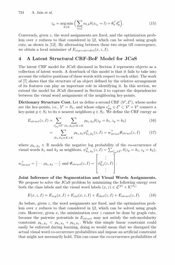
4 A Latent Structural CRF-BoF Model for JCaS

The latent CRF model for JCaS discussed in Section 3 represents objects as acollection of latent words. A drawback of this model is that it fails to take intoaccount the relative positions of these words with respect to each other. The workof [7] shows that the structure of an object defined by the relative arrangementof its features can play an important role in identifying it. In this section, weextend the model for JCaS discussed in Section 3 to capture the dependenciesbetween the visual word assignments of the neighboring key-points.

Dictionary Structure Cost. Let us define a second CRF (V ′, E ′), whose nodesare the key-points, i.e., V ′ = SI , and whose edges e′pq ∈ E ′ ⊂ V ′ × V ′ connect akey-point p ∈ SI to its n nearest neighbors q ∈ SI . We define the CRF energy as

Estruct(z, I) =∑

e′pq∈E′

∑

(k1,k2)∈K×Kρk1,k2δ(zp = k1, zq = k2) (16)

=∑

(k1,k2)∈K×Kρk1,k2ψ

Sk1,k2

(z, I) = w�structΨstruct(z, I) (17)

where ρk1,k2 ∈ R models the negative log probability of the co-occurrence ofvisual words k1 and k2 as neighbors, ψS

k1,k2(z, I) =

∑e′pq∈E′ δ(zp = k1, zq = k2),

w�struct =

[· · · ρk1,k2 · · ·] and Ψstruct(z, I) =

⎡

⎢⎢⎣

...φSk,l(z, I)

...

⎤

⎥⎥⎦.

Joint Inference of the Segmentation and Visual Words Assignments.We propose to solve the JCaS problem by minimizing the following energy overboth the class labels and the visual word labels (x, z) ∈ L|V| ×K|SI |

E(x, z, I) = Eseg(x, I) + Ecat(x, z, I) + Edict(z, I) + Estruct(z, I). (18)

As before, given z, the word assignments are fixed, and the optimization prob-lem over x reduces to that considered in §2, which can be solved using graphcuts. However, given x, the minimization over z cannot be done by graph cuts,because the pairwise potentials in Estruct may not satisfy the sub-modularityconstraint ρk1,k2 < ρk1,k3 + ρk3,k1 . While this simple linear constraint couldeasily be enforced during learning, doing so would mean that we disregard theactual visual word co-occurrence probabilities and impose an artificial constraintthat might not necessarily hold. This can cause the co-occurrence probabilities of


visual words to result in a model which is not coherent with the object structure.Therefore, we choose not to impose these constraints on the parameters and re-sort to loopy-belief propagation techniques [23, 24] for computing the optimal zgiven x. We alternate these two steps till convergence to a local minimum.

5 Max-Margin Learning Using Latent SVMs

So far, we have proposed a new framework for JCaS based on minimizing theenergy E(x, z, I) = w�Ψ(x, z, I). As shown in §3 and §4, this problem can besolved using graph cuts and/or loopy-belief propagation.

In this section, we consider the learning problem. That is, given a collectionof training images {Ij}Nj=1 and their corresponding ground-truth segmentations

{xj}Nj=1, our goal is to learn the parameters w. The main challenge is that we do

not know the latent variables {zj}Nj=1. We address this problem using the latentstructural SVM framework proposed in [25]. In this framework, the parametersw are learnt using an iterative algorithm that alternates between solving for thelatent variables zj given the energy parameters w, and solving for the parametersw given the latent variables. More specifically, the algorithm proceeds as follows:

– Step 1: Given a current estimate of the energy parameters w, compute anestimate zj of the latent variables as

zj = argminz∈K|S

Ij|w�Ψ(xj , z, Ij) ∀j ∈ {1, · · · , N}. (19)

– Step 2: Given an estimate zj of the latent variables, learn w by solving thefollowing structural SVM training problem [22]

{w∗, {ξ∗j }Nj=1} = argminw,{ξj}Nj=1

1

2‖w‖2 + μ

N

N∑

j=1

ξj , subject to

(a) ∀i = 1, . . . , N : ∀(x, z) ∈ L|V| ×K|SI | :

w�(Ψ(x, z; Ij)− Ψ(xj , zj; Ij)) ≥ Δ(x, xj)− ξj ,

(b) ∀i = 1, . . . , N : ξi ≥ 0 and (c) w ≥ 0.

(20)

In step 2, we want to learn the parameter vector w such that the value of Efor the ground truth segmentation x and imputed word assignments z is smallerthan its value for other possible labellings and words assignments, i.e., ∀(x, z) ∈L|V| × K|SI | \ (x, z), E(x, z, I) < E(x, z, I). However, all wrong segmentationsand assignments can not be penalized equally. For example, a segmentation thatlabels one superpixel wrong is better than one that labels 80% of the superpixelswrong. The loss function Δ(x, x) measures the deviation of a given segmentationfrom the ground truth as

Δ(x, x) =d(x, x)

|x| , (21)

where d(x, x) measures the number of sites which have different labels in x and x.Finally, ξj represents the slack variable for training example j. The introductionof slack variables is necessary because, otherwise, there may not be a set ofparameters w that satisfies all the constraints described in (20).

726 A. Jain et al.

We refer the reader to [22] for the details of the cutting plane method usedto solve this optimization problem efficiently.

6 Experiments

Datasets. We performed our experiments on the Graz-02 dataset [26] and theCamVid dataset [27]. The Graz dataset contains 900 images of bikes, humans andcars. 450 images were used for training and the rest of the images were used fortesting. The CamVid dataset has 700 labelled images out of which we used 350for training and 350 for testing. The CamVid dataset has been annotated into32 classes out of which we chose the 11 classes that were considered in [28]. Also,to make our results comparable with prior work, we down-sampled the imagesby 1/3 and did not consider the void class. For both databases, we created thesuperpixels using the quickshift method [19].

Metrics. We compared the different methods using two performance metrics.The pixel accuracy is the percentage of correctly labeled pixels per image aver-aged over all the images. The intersection/union metric considers not only thetrue positives (TP), but also the false positives (FP) and false negatives (FN).For each image, the intersection/union metric is computed as 100×#TP

#TP+#FP+#FN .

Methods and Baselines. We compared the following methods:

1. CRF-U: this is a simplified version of the method described in Section 2,which uses only the unary segmentation cost. This method is a particularcase of that in [6]. We report results from our implementation.

2. CRF-UP: this is a simplified version of the method described in Section2, which uses only the unary and pairwise segmentation costs. This is themethod proposed in [6]. We report results from our implementation.

3. CRF-BoF-L: this method is described in Section 2. It uses a CRF model witha BoF categorization cost constructed using linear classifiers. This method isa particular case of that in [12]. We report results from our implementation.

4. CRF-BoF-IK: this is the method proposed in [12], which uses a CRF modelwith a BoF categorization cost constructed using kernel-SVM classifiers withthe intersection kernel. We report results from [12].

5. LCRF-BoF-L: this method is described in Section 3. It uses a latent CRFmodel with a BoF cost with linear classifiers plus a dictionary learning cost.

6. SLCRF-BoF-L: this method is described in Section 4. It uses a latent CRFmodel with a BoF cost with linear classifiers plus a structured dictionarylearning cost.

Implementation Details. The parameters of the unary segmentation cost arechosen as follows. The size of the superpixel neighborhood used to define thefeatures for the unary classifiers is set to τ = 8. The number of visual words isset to |K| = 400. The parameter of the RBF kernel is set to γ = 1/ξ20.25, whereξ20.25 is the first quartile of the ξ2 distances in the training set. The parameterof the categorization cost is set to |K| = 20 visual words. The parameter of thestructural SVM learning method is set to μ = 106.


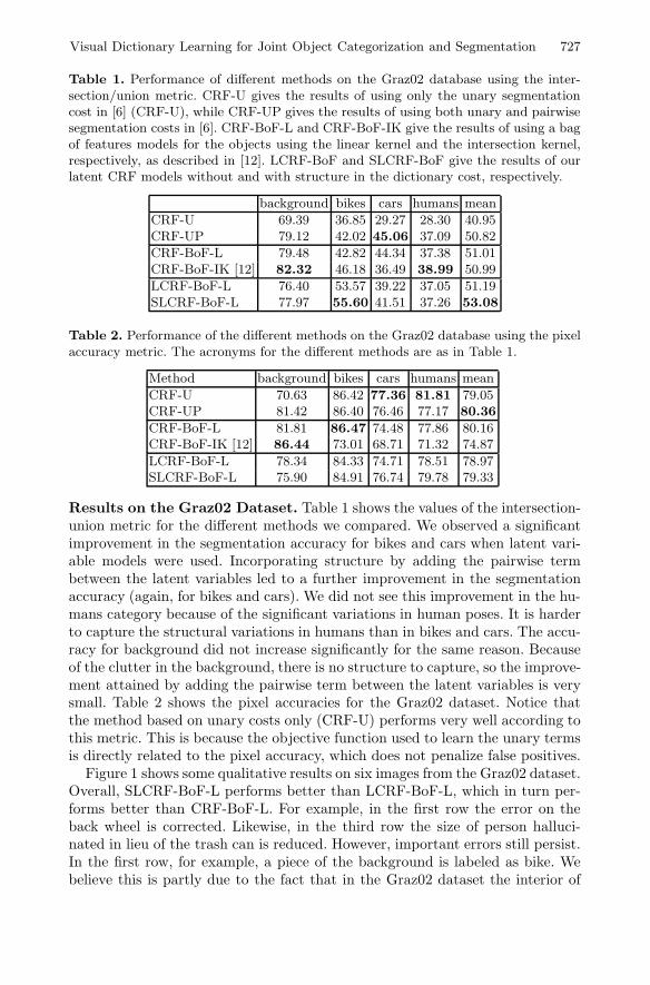
Table 1. Performance of different methods on the Graz02 database using the inter-section/union metric. CRF-U gives the results of using only the unary segmentationcost in [6] (CRF-U), while CRF-UP gives the results of using both unary and pairwisesegmentation costs in [6]. CRF-BoF-L and CRF-BoF-IK give the results of using a bagof features models for the objects using the linear kernel and the intersection kernel,respectively, as described in [12]. LCRF-BoF and SLCRF-BoF give the results of ourlatent CRF models without and with structure in the dictionary cost, respectively.

background bikes cars humans mean

CRF-U 69.39 36.85 29.27 28.30 40.95CRF-UP 79.12 42.02 45.06 37.09 50.82

CRF-BoF-L 79.48 42.82 44.34 37.38 51.01CRF-BoF-IK [12] 82.32 46.18 36.49 38.99 50.99

LCRF-BoF-L 76.40 53.57 39.22 37.05 51.19SLCRF-BoF-L 77.97 55.60 41.51 37.26 53.08

Table 2. Performance of the different methods on the Graz02 database using the pixelaccuracy metric. The acronyms for the different methods are as in Table 1.

Method background bikes cars humans mean

CRF-U 70.63 86.42 77.36 81.81 79.05CRF-UP 81.42 86.40 76.46 77.17 80.36

CRF-BoF-L 81.81 86.47 74.48 77.86 80.16CRF-BoF-IK [12] 86.44 73.01 68.71 71.32 74.87

LCRF-BoF-L 78.34 84.33 74.71 78.51 78.97SLCRF-BoF-L 75.90 84.91 76.74 79.78 79.33

Results on the Graz02 Dataset. Table 1 shows the values of the intersection-union metric for the different methods we compared. We observed a significantimprovement in the segmentation accuracy for bikes and cars when latent vari-able models were used. Incorporating structure by adding the pairwise termbetween the latent variables led to a further improvement in the segmentationaccuracy (again, for bikes and cars). We did not see this improvement in the hu-mans category because of the significant variations in human poses. It is harderto capture the structural variations in humans than in bikes and cars. The accu-racy for background did not increase significantly for the same reason. Becauseof the clutter in the background, there is no structure to capture, so the improve-ment attained by adding the pairwise term between the latent variables is verysmall. Table 2 shows the pixel accuracies for the Graz02 dataset. Notice thatthe method based on unary costs only (CRF-U) performs very well according tothis metric. This is because the objective function used to learn the unary termsis directly related to the pixel accuracy, which does not penalize false positives.

Figure 1 shows some qualitative results on six images from the Graz02 dataset.Overall, SLCRF-BoF-L performs better than LCRF-BoF-L, which in turn per-forms better than CRF-BoF-L. For example, in the first row the error on theback wheel is corrected. Likewise, in the third row the size of person halluci-nated in lieu of the trash can is reduced. However, important errors still persist.In the first row, for example, a piece of the background is labeled as bike. Webelieve this is partly due to the fact that in the Graz02 dataset the interior of

728 A. Jain et al.

Image Ground Truth CRF-BoF-L LCRF-BoF-L SLCRF-BoF-L

Fig. 1. JCaS results for the Graz-02 dataset: Background, bikes, cars and humans arecolor coded as red, green, blue and yellow respectively

the wheels is labeled as bike, while the background is also visible. This may alsobe the cause for the erroneous segmentation of the bikes in the second row.

Results on the CamVid Dataset. Since the CamVid dataset has 11 classes,we could not run the experiments using the CRF-BoF-IK method proposed in[12], because the optimization with graph cuts became prohibitive due to thenumber of auxiliary variables needed to implement the intersection kernel. Table3 shows the values of the intersection-union metric for the remaining methods.We observed that for objects with a clearly defined structure, such as cars, signsand buildings, the proposed latent models (LCRF-BoF-L and SLCRF-BoF-L)performed well. However for textured objects such as sky, road and fence, thepurely bottom-up methods (CRF-U and CRF-UP) gave better results, becausethe top-down cost captures an object model that is not very relevant for such.Overall, SLCRF-BoF-L is not as effective as LCRF-BoF-L because of the absenceof structure in object categories like sky. This leads to very bad results for the


Table 3. Performance of different methods on the CamVid database using the inter-section/union metric. The acronyms for the different methods are as in Table 1.

Bldg Roads Tree Sky Car Ped Fence Col. SW Bike Sign MeanCRF-U 46.84 68.03 43.26 54.84 27.75 6.33 24.53 2.84 35.73 16.50 5.50 30.20CRF-UP 51.61 74.96 46.61 65.54 31.09 7.43 27.94 3.33 39.47 17.83 7.21 33.91CRF-BoF-L 42.95 40.53 38.96 48.55 12.79 6.19 9.47 1.58 17.18 4.67 1.17 20.37LCRF-BoF-L 48.73 72.22 52.01 45.58 37.15 9.79 23.64 8.62 33.88 29.35 12.18 33.92SLCRF-BoF-L 51.91 53.75 48.84 34.09 37.18 9.90 23.21 8.09 23.00 28.87 14.80 30.33

Table 4. Performance of the different methods on the CamVid database using thepixel accuracy metric. The acronyms for the different methods are as in Table 1.

Method Bldg Roads Tree Sky Car Ped Fence Col. SW Bike Sign MeanCRF-U 52.35 71.89 60.14 64.91 54.05 42.44 59.06 15.25 71.83 65.22 40.76 54.36CRF-UP 56.18 80.16 61.43 77.08 53.86 41.10 60.60 15.97 73.39 60.16 41.59 56.50CRF-BoF-L 47.98 42.05 59.50 56.74 15.14 13.62 35.33 17.54 51.11 60.86 38.72 39.87LCRF-BoF-L 51.65 80.30 65.73 74.47 53.47 49.75 56.45 28.77 71.75 73.70 46.37 59.31SLCRF-BoF-L 55.60 60.01 65.37 54.82 55.02 43.62 52.21 28.50 70.11 71.68 44.03 54.63STL [28] 68.90 82.10 79.30 96.70 54.10 18.20 43.10 1.00 75.90 40.80 19.10 54.652D-3D [29] 71.10 88.40 56.10 89.50 76.50 59.10 4.80 11.40 84.70 28.10 12.50 52.99

SLCRF-BoF-L method because it tries to model the structure of these categories,which leads to over-fitting.

Table 4 shows the values of the pixel accuracies for the CamVid database.In this case, we also compare our results to those obtained using supervisedlabel transfer (STL) [28] and joint 2D-3D segmentation of street scenes (2D-3D)[29]. For textured classes such as trees, road and sky, STL performs better thanthe latent variable models. However, on structured objects such as bikes andcars, 2D-3D performs better because it captures the 3D structure of the object.The overall performance of these methods is worse than that of LCRF-BoF-Lbecause they perform very poorly for certain classes, while LCRF-BoF-L andSLCRF-BoF-L are more consistent in their performance.

Finally, Figure 2 shows some qualitative results on two images from theCamVid dataset. Overall, SLCRF-BoF-L performs slightly better than LCRF-BoF-L, which in turn performs better than CRF-BoF-L.

Image Ground Truth CRF-BoF-L LCRF-BoF SLCRF-BoF

Fig. 2. JCaS results for the CamVid dataset: buildings, roads, tree, sky, car, pedestrian,fence, column, sidewalk, bike, sign are color coded as dark red, light purple, green, gray,dark purple, dark green, dark blue, light green, blue, sky blue, and pink, respectively.

730 A. Jain et al.

7 Conclusion

We have shown that learning a task specific dictionary jointly with the clas-sification and segmentation parameters leads to a significant improvement inthe accuracy of the results. Our experiments suggest that for object classeswhere spatial context is important, using context-based dictionary learning (la-tent CRFs with connected hidden variables) increases the accuracy of results.However, for classes such as sky or fence, which do not have a fixed structure,context-based dictionary learning leads to inaccurate segmentations.

In future work, it would be interesting to identify the set of object modelswhich can be used along with the latent CRF formulation for JCaS. A compar-ison of the results of task specific context dependent dictionary learning withdifferent kinds of neighborhood structures (not just nearest neighbors) can pro-vide us with more accurate object models and better segmentations. Identifyingthe neighborhood structures and potentials which would allow us to use fasterinference techniques (unlike loopy belief propagation) and studying the effectsof using a different feature descriptor or a combination of feature descriptors forthe interest points are other promising directions.

Acknowledgments. This work was partially supported by grants DARPAFA8650-11-1-7153, ONR N00014-09-10839, NSF 1004782.

References

1. Winn, J.M., Shotton, J.: The layout consistent random field for recognizing andsegmenting partially occluded objects. In: IEEE Conf. on Computer Vision andPattern Recognition, pp. 37–44 (2006)

2. Larlus, D., Jurie, F.: Combining appearance models and Markov random fieldsfor category level object segmentation. In: IEEE Conf. on Computer Vision andPattern Recognition (2008)

3. Shotton, J., Johnson, M., Cipolla, R.: Semantic texton forests for image cate-gorization and segmentation. In: IEEE Conf. on Computer Vision and PatternRecognition (2008)

4. Galleguillos, C., Rabinovich, A., Belongie, S.: Object categorization using co-occurrence, location and appearance. In: IEEE Conf. on Computer Vision andPattern Recognition (2008)

5. Gould, S., Gao, T., Koller, D.: Region-based segmentation and object detection.In: Neural Information Processing Systems (2009)

6. Fulkerson, B., Vedaldi, A., Soatto, S.: Class segmentation and object localizationwith superpixel neighborhoods. In: IEEE Int. Conf. on Computer Vision (2009)

7. Micusik, B., Kosecka, J.: Semantic segmentation of street scenes by superpixel co-occurrence and 3d geometry. In: IEEE Workshop on Video-Oriented Object andEvent Classification (2009)

8. Ladicky, L., Russell, C., Kohli, P., Torr, P.: Associative hierarchical CRFs forobject class image segmentation. In: IEEE Int. Conf. on Computer Vision (2009)

9. Lempitsky, V.S., Vedaldi, A., Zisserman, A.: A pylon model for semantic segmen-tation. In: Neural Information Processing Systems (2011)

10. Russell, C., Ladicky, L., Kohli, P., Torr, P.: Graph Cut Based Inference with Co-occurrence Statistics. In: Daniilidis, K., Maragos, P., Paragios, N. (eds.) ECCV2010, Part V. LNCS, vol. 6315, pp. 239–253. Springer, Heidelberg (2010)


11. Verbeek, J., Triggs, B.: Scene segmentation with CRFs learned from partiallylabeled images. In: Neural Information Processing Systems (2008)

12. Singaraju, D., Vidal, R.: Using global bag of features models in random fields forjoint categorization and segmentation of objects. In: IEEE Conference on Com-puter Vision and Pattern Recognition (2011)

13. Sivic, J., Zisserman, A.: Video google: A text retrieval approach to object matchingin videos. In: IEEE International Conference on Computer Vision, pp. 1470–1477(2003)

14. Dance, C., Willamowski, J., Fan, L., Bray, C., Csurka, G.: Visual categorizationwith bags of keypoints. In: European Conference on Computer Vision (2004)

15. Winn, J.M., Criminisi, A., Minka, T.P.: Object categorization by learned universalvisual dictionary. In: IEEE International Conference on Computer Vision (2005)

16. Moosmann, F., Triggs, B., Jurie, F.: Fast discriminative visual codebooks usingrandomized clustering forests. In: Neural Information Processing Systems, vol. 19,pp. 985–991 (2007)

17. Yang, L., Jin, R., Sukthankar, R., Jurie, F., Yang, L., Jin, R., Sukthankar, R., Jurie,F.: Unifying discriminative visual codebook generation with classifier training forobject category recognition. In: IEEE Conference on Computer Vision and PatternRecognition (2008)

18. Yang, J., Yang, M.: Top-down visual saliency via joint crf and dictionary learning.In: IEEE Conference on Computer Vision and Pattern Recognition (2012)

19. Vedaldi, A., Soatto, S.: Quick Shift and Kernel Methods for Mode Seeking. In:Forsyth, D., Torr, P., Zisserman, A. (eds.) ECCV 2008, Part IV. LNCS, vol. 5305,pp. 705–718. Springer, Heidelberg (2008)

20. Kolmogorov, V., Zabih, R.: What Energy Functions Can Be Minimized Via GraphCuts? IEEE Trans. on Pattern Analysis and Machine Intelligence 26, 147–159(2004)

21. Kohli, P., Ladicky, L., Torr, P.H.S.: Robust higher order potentials for enforcinglabel consistency. International Journal of Computer Vision 82, 302–324 (2009)

22. Tsochantaridis, I., Joachims, T., Hofmann, T., Altun, Y.: Large margin methodsfor structured and interdependent output variables. Journal of Machine LearningResearch 6, 1453–1484 (2005)

23. Murphy, K.P., Weiss, Y., Jordan, M.I.: Loopy belief propagation for approximateinference: An empirical study. In: Proceedings of Uncertainty in AI, pp. 467–475(1999)

24. Pearl, J.: Probabilistic reasoning in intelligent systems: networks of plausible in-ference. Morgan Kaufmann Publishers Inc., San Francisco (1988)

25. Yu, C.N.J., Joachims, T.: Learning structural svms with latent variables. In: In-ternational Conference on Machine Learning, ICML (2009)

26. Opelt, A., Pinz, A.: The TU Graz-02 database (2002),http://www.emt.tugraz.at/~pinz/data/GRAZ_02/

27. Brostow, G.J., Shotton, J., Fauqueur, J., Cipolla, R.: Segmentation and Recogni-tion Using Structure from Motion Point Clouds. In: Forsyth, D., Torr, P., Zisser-man, A. (eds.) ECCV 2008, Part I. LNCS, vol. 5302, pp. 44–57. Springer, Heidel-berg (2008)

28. Zhang, H., Xiao, J., Quan, L.: Supervised Label Transfer for Semantic Segmen-tation of Street Scenes. In: Daniilidis, K., Maragos, P., Paragios, N. (eds.) ECCV2010, Part V. LNCS, vol. 6315, pp. 561–574. Springer, Heidelberg (2010)

29. Floros, G., Leibe, B.: Joint 2D-3D temporally consistent semantic segmentation of

street scenes. In: IEEE Conference on Computer Vision and Pattern Recognition

(2012)

http://www.emt.tugraz.at/~pinz/data/GRAZ_02/

visual dictionary learning for joint object -

Documents