visual quantum mechanics - home page of...

Visual Quantum MechanicsBernd ThallerInstitute for Mathematics, University of Graz, Heinrichstrasse 36, A-8010 Graz, Austria

"Visual Quantum Mechanics" is a large collection of Mathematica-generated movies showing quantum-mechanical phenomena. A set of Mathematica packages and associated notebooks help to solve the Schrödinger or Dirac equation, visualize complex-valued and spinor-valued functions, compute their Fourier transform, etc. This article presents a few examples showing different types of visualizations and discusses their usefulness for pedagogic purposes. The application of innovative visualization techniques is particularly rewarding in the field of quantum mechanics, where computer graphics allows us to depict phenomena that cannot be seen by any other means. It is the goal to provide an intuitive feeling of quantum mechanics which is important for a deeper understanding but cannot be gained easily by studying the theory in the conventional manner. Visual Quantum Mechanics thus makes complicated phenomena more comprehensible and offers new insights even for the advanced student or researcher.

‡ Quantum mechanics - why visualizations?The very concept of "looking like something" makes no sense in the strange world of electrons. Quantum mechanics describes that reality in terms of rather abstract concepts like wave functions. Here we present some methods to visualize wave functions with the help of Mathematica. The reader has to be aware that the images do not show objects that exist in the same sense as a coconut exists. More or less intuitive interpretation rules tell us in what sense the visual representations are linked to the result of possible experiments. It goes far beyond the scope of this article to derive these interpretation rules, and the interested reader is referred to the literature [1].

This article shows a few examples from the project "Visual Quantum Mechanics". Two books on elementary and advanced quantum mechanics with accompanying CD-ROMs [1, 2] contain several hundreds of QuickTime movies exported from Mathematica notebooks. Though pre-fabricated and not interactive, those movies serve an important didactic purpose: They provide the phenomenological background for the theory, and they help to obtain an intuitive feeling for wave functions that is so hard to obtain from the mathematical formulas alone. They motivate students to dig deeper into the theory and the phenomena visible in the movies indeed draw the attention towards advanced topics normally not dealt with in textbooks (see Figure 1). The collection of visualizations has earned the European Academic Software Award in 2000 and in 2004. More information is on the project's web site at http://vqm.uni-graz.at.

Avignon, June 2006 8th International Mathematica Symposium

Figure 1. Pre-fabricated, Mathematica-generated QuickTime movie in Visual Quantum Mechanics [2])

The Mathematica source of the animations is provided as well and thus it is easy to recreate the movies with other parameters and/or initial conditions in order to explore a phenomenon more interactively. It can bring enormous benefit to let students do their own visualization projects. In order to produce a useful visualization, one has to analyze a quantum system in depth, and one is likely to learn something new even in the case of very simple systems. This active and explorative approach lets students go far beyond conventional textbook knowledge.

There are, however, some caveats. One is that many computations in quantum mechanics are rather time consuming, and often personal computers are still too slow to perform simulations of realistic quantum processes within a reasonable time. Another problem is the inherent difficulty of quantum mechanics. For every situation, one has to determine the scale of space and time and energy together with suitable ranges of the parameters where something interesting is going to happen, and common sense or everyday experience is not going to help. The number of possibilities is very large, and if one chooses the wrong parameter values, nothing can be seen that is easily interpreted. Usually, this asks too much of a beginner and I would recommend that approach only for advanced students who are already familiar with both Mathematica and the foundations of quantum mechanics.

2 Bernd Thaller

8th International Mathematica Symposium Avignon, June 2006

‡ Visualizations in quantum mechanics - why colors?The propagation of particles through space has hidden wave-like properties. By ‘hidden’ we mean that the wave cannot be observed directly, but only through interference. An example is shown in Figure 2.

Figure 2. (a) Interference of classical waves and (b) interference of densities in beams of particles.

The image to the left (Figure 2a) shows two classical wave trains meeting at a certain angle. Their wave-like nature is visible everywhere, not only in the overlap region where we observe an interference pattern - a change in the direction of the wave fronts and a periodic variation of the intensity. In the simplest case, the interference pattern can be explained by linear superposition (addition) of the two waves.

Apparently, interference also happens in the second image (Figure 2b), but its origin is not visible. This image depicts two overlapping beams of elementary particles. The density of particles in each beam is constant and very thin (in order to exclude interactions between the particles). This constant density is visualized by a constant shade of gray (with black corresponding to no particles at all). The periodic variation of the particle density in the overlap region is quite extraordinary, because in classical physics one would expect that (in the absence of interaction) the particle densities are just added whenever two beams are superimposed.

The interference of particle densities is not easy to observe. One condition is that the two beams originate from a common source and that the particles in the beam are not disturbed by attempts to determine their position in one of the beams before they reach the interference region. Experimental setups such as the double-slit experiment are designed to meet these conditions and are nowadays routinely performed by experimental physicists, not only for bosonic particles (light beams) but also for fermionic particles (electron beams). Within the individual beams we observe no wave-like behavior whatsoever. What causes the interference of particle beams? It is not a new form of interaction between particles, because the interference does not depend on the particle density in the beam. In extreme cases, the population of the beams might be so thin, that a single particle travels along the beam every once in a while. The density variations can still be measured by counting particles over a longer time. The interference pattern is just the spatial variation in the number of detected particles, that is, the spatial variation of the position probability.

It turns out that the interference pattern formed by particles with a certain momentum p is identical to the periodic variations of the intensity in a superposition of waves with a wave length l = 2p—/p. Therefore, one associates a wave phenomenon of that wave length with the motion of a particle with momentum p. One describes the position probability with the intensity (square of the absolute value) of the wave and assumes that the phase is not observable, except in an indirect way through interference.

Notice that a wave where the absolute value is independent of the phase must be described at least by a two-dimensional wave quantity. It is thus quite natural to assume that the wave quantity is a complex number. A complex number is a two-dimensional object, characterized by an absolute value and a phase. The (square of the) absolute value is chosen to describe the position probability density, while the phase is assumed to be not directly observable. A particle with momentum p (in dimensionless units with m=—=1) would thus be described by the wave

Visual Quantum Mechanics 3


The image to the left (Figure 2a) shows two classical wave trains meeting at a certain angle. Their wave-like nature is visible everywhere, not only in the overlap region where we observe an interference pattern - a change in the direction of the wave fronts and a periodic variation of the intensity. In the simplest case, the interference pattern can be explained by linear superposition (addition) of the two waves.

Apparently, interference also happens in the second image (Figure 2b), but its origin is not visible. This image depicts two overlapping beams of elementary particles. The density of particles in each beam is constant and very thin (in order to exclude interactions between the particles). This constant density is visualized by a constant shade of gray (with black corresponding to no particles at all). The periodic variation of the particle density in the overlap region is quite extraordinary, because in classical physics one would expect that (in the absence of interaction) the particle densities are just added whenever two beams are superimposed.

The interference of particle densities is not easy to observe. One condition is that the two beams originate from a common source and that the particles in the beam are not disturbed by attempts to determine their position in one of the beams before they reach the interference region. Experimental setups such as the double-slit experiment are designed to meet these conditions and are nowadays routinely performed by experimental physicists, not only for bosonic particles (light beams) but also for fermionic particles (electron beams). Within the individual beams we observe no wave-like behavior whatsoever. What causes the interference of particle beams? It is not a new form of interaction between particles, because the interference does not depend on the particle density in the beam. In extreme cases, the population of the beams might be so thin, that a single particle travels along the beam every once in a while. The density variations can still be measured by counting particles over a longer time. The interference pattern is just the spatial variation in the number of detected particles, that is, the spatial variation of the position probability.

It turns out that the interference pattern formed by particles with a certain momentum p is identical to the periodic variations of the intensity in a superposition of waves with a wave length l = 2p—/p. Therefore, one associates a wave phenomenon of that wave length with the motion of a particle with momentum p. One describes the position probability with the intensity (square of the absolute value) of the wave and assumes that the phase is not observable, except in an indirect way through interference.

Notice that a wave where the absolute value is independent of the phase must be described at least by a two-dimensional wave quantity. It is thus quite natural to assume that the wave quantity is a complex number. A complex number is a two-dimensional object, characterized by an absolute value and a phase. The (square of the) absolute value is chosen to describe the position probability density, while the phase is assumed to be not directly observable. A particle with momentum p (in dimensionless units with m=—=1) would thus be described by the wave

(1)y@x, tD = ‰i Ip x- p2 tÅÅÅÅÅÅÅÅÅ2 MA low-density beam of particles is described by the same wave function. The beam just provides a larger sample of independent identically prepared particles, e.g., for the measurement of position probabilities.

In general, a wave function describing the propagation of a particle is a solution of a quantum-mechanical evolution equation. For free, spinless, non-relativistic particles this is the free Schrödinger equation. In dimensionless units, this equation reads

(2)Â ∂t y@x, tD = -1ÅÅÅÅ2 ∂8x,2< y@x, tD

and its solutions are complex-valued function. Functions with complex values are best visualized using colors.

‡ Wave functions and colorsThe standard package Graphics`ArgColors` by Roman Maeder defines colors for the argument of complex numbers. By adding the dimension of brightness, this can easily extended to a unique coloring of the whole complex plane. In that way, we obtain the color map shown in Figure 3. It has been described in detail in Ref. [3].

4 Bernd Thaller


Figure 3. Complex plane with colors determined by phase (hue) and absolute value (lightness).

This image shows the complex plane with a unique color associated to each point. The lines of constant phase/hue are the radial lines and the lines with constant absolute value/brightness are the circles. The origin (the complex number 0) becomes black and infinity becomes white. The negative of a complex number always has the complementary color, for example, positive real numbers are red, negative real numbers are cyan., We note that the vector addition in the complex plane (i.e., the addition of complex numbers) may be interpreted in terms of color mixing. For example, adding red light and green light produces light that is perceived as yellow, although the wavelength of yellow does not occur in the mixture. Moreover, adding similar colors result in a color that is brighter, while complementary colors tend to cancel each other. (Actually, colors behave in a more complex way, as there is additive and subtractive mixing of colors.)

Using these rules of color addition, we can produce a nice image of the complex waves describing the interference of position densities in particle beams. The following image Figure 4 explains the interference in Figure 1 by assuming that a beam of constant particle density is actually a wave with a constant intensity and a periodic phase. When superimposing two such beams, the colors are added according to vector addition in the colored complex plane.



Figure 4. Interference of waves with constant intensity (brightness). The wave nature is described by a periodically changing color. Interference is created by the rules of color mixing defined through vector addition in the colored plane of Figure 3.

Technically, the color variable interpolating between black and white is called lightness. The standard package Graphics`Colors` defines the function HLSColor which defines colors in terms of hue, lightness and saturation. The colors in Figure 3 all have maximal saturation, so they are on the surface of the color manifold, which may be envisaged as a sphere in three dimensions. The color map of the complex plane is finally obtained by stereographic projection from this sphere onto the complex plane [1,3].

‡ The VQM packagesFor the visualization of wave functions in quantum mechanics, I have been using the phase-coloring method to plot wave functions since 1994, and several Mathematica packages have been developed for that purpose. Presently, the collection consist of 14 packages that can be downloaded from the project's web page. They are work in progress and not yet complete, but fully functional. These packages deal with the most common visualization tasks, solve the Schrödinger equation numerically, help to compute the Fourier transform, provide exact solutions, e.g., to harmonic-oscillator and Coulomb problems, help to manipulate and plot spin states, or decompose solutions of the one-dimensional Dirac equation into parts with positive and negative energy. We cannot go into the details here and refer to the notebooks coming with Advanced Visual Quantum Mechanics [2] for examples of the usage of these packages. Here we describe just a few of them.

When these packages are installed, all symbols can be loaded at once by<< VQM`

The strategy of solving the Schrödinger equation in one and two space dimensions is based on implementing a fast direct solver in an external C++ program "QuantumKernel", that communicates via MathLink with the Mathematica kernel. The package VQM`QuantumKernel` defines the interface to the Schrödinger equation solver. It uses a simple Crank-Nicolson formula for the solution in one space dimension. In two dimensions, we use a variation of theTrotter-Suzuki method [3].

The decision against the built-in Mathematica routines has been made at an early stage of the project. Meanwhile, NDSolve has made significant progress, but the problem is that it keeps the whole solution as an interpolating function object which makes it too memory-hungry and which is not necessary in order to produce an animation step-by-step. In contrast, we keep only the information needed for one time step, and visualize the solution at each time step immediately. Hence the size of the animation is essentially only limited by the memory available for the notebook containing the graphics cells.

Whatever approach one chooses when solving the Schrödinger equation, one immediately faces the problem that the solutions are complex-valued functions and cannot be visualized easily. Therefore, several of the VQM-packages deal with visualization. The package VQM`ColorMaps` defines the various color maps for complex numbers or vectors, VQM`ArgColorPlot` provides methods for visualizing wave packets and spinor-valued wave packets in one dimension, VQM`ComplexPlot` fulfills similar tasks in two dimensions. VQM`QGraphics2D` is a package for gathering and visualizing the output from the external C++ program QuantumKernel.

The package VQM`ArgColorPlot` provides a functionality similar to that of the standard package Graphcis`FilledPlot`, but it allows to fill the space between the curve and the x-axis with a variable color. It depicts a complex-valued function of a single real variable by plotting a curve representing the absolute value of the function and filling it with a color describing the phase of the complex value at every point according to the color circle described above. For example, here we plot a Gaussian wave packet (a minimal uncertainty wave packet typically used as an initial condition in quantum mechanics) describing a particle with average momentum 6 and average position 0:

6 Bernd Thaller


The strategy of solving the Schrödinger equation in one and two space dimensions is based on implementing a fast direct solver in an external C++ program "QuantumKernel", that communicates via MathLink with the Mathematica kernel. The package VQM`QuantumKernel` defines the interface to the Schrödinger equation solver. It uses a simple Crank-Nicolson formula for the solution in one space dimension. In two dimensions, we use a variation of theTrotter-Suzuki method [3].

The decision against the built-in Mathematica routines has been made at an early stage of the project. Meanwhile, NDSolve has made significant progress, but the problem is that it keeps the whole solution as an interpolating function object which makes it too memory-hungry and which is not necessary in order to produce an animation step-by-step. In contrast, we keep only the information needed for one time step, and visualize the solution at each time step immediately. Hence the size of the animation is essentially only limited by the memory available for the notebook containing the graphics cells.

Whatever approach one chooses when solving the Schrödinger equation, one immediately faces the problem that the solutions are complex-valued functions and cannot be visualized easily. Therefore, several of the VQM-packages deal with visualization. The package VQM`ColorMaps` defines the various color maps for complex numbers or vectors, VQMÀrgColorPlot` provides methods for visualizing wave packets and spinor-valued wave packets in one dimension, VQM`ComplexPlot` fulfills similar tasks in two dimensions. VQM`QGraphics2D` is a package for gathering and visualizing the output from the external C++ program QuantumKernel.

The package VQMÀrgColorPlot` provides a functionality similar to that of the standard package Graphcis`FilledPlot`, but it allows to fill the space between the curve and the x-axis with a variable color. It depicts a complex-valued function of a single real variable by plotting a curve representing the absolute value of the function and filling it with a color describing the phase of the complex value at every point according to the color circle described above. For example, here we plot a Gaussian wave packet (a minimal uncertainty wave packet typically used as an initial condition in quantum mechanics) describing a particle with average momentum 6 and average position 0:

QArgColorPlot@Exp@6 I x - x^2 ê 2D, 8x, -4, 4<D

Ü Graphics Ü

The distance between the positions with the same color corresponds to the deBroglie wave length of the particle in dimensionless units. Even from the still image, we learn a lot about the dynamical state of this particle by looking at the colors. The average velocity of this wave packet is related to the wave length (the shorter the wave length, the faster the particle). The direction of motion is given by the positive (counter-clockwise) direction in the color circle, that is, in the direction from red to yellow to green, etc. Thus, the direction of motion can be read off from the order of the colors in the image (in this case, from left to right). This is a distinct advantage of the phase coloring method in comparison to visualization methods that show only the position probability density or only real- and imaginary parts of the wave function.

In the following, we present a typical elementary application that combines the functionalities of the packages VQM`QuantumKernel` for solving the Schrödinger equation,, VQMÀrgColorPlot` for visualizing the result, and VQM`FastFourier` for computing the Fourier transform.

It is very instructive to show a wave function describing the position distribution together with its Fourier transform, which describes the momentum distribution. In dimensionless coordinates (particles with mass 1) and in non-relativistic quantum mechanics, the momentum distribution is identical with the velocity distribution and thus easy to interpret.

Figure 5 shows a snapshot from the time evolution of a wave packet in the process of being scattered at a potential well. (See [5] for an animated version of this image as well as of the other visualizations in this article.) The upper image of Figure 5 shows the wave packet in position space and indicates the potential well. The wave packet, initially coming in from the left and moving to the right, has already split into a larger part transmitted to the right, and a smaller reflected part that is thrown back to the left. Inside the well, rapid oscillations occur.



The distance between the positions with the same color corresponds to the deBroglie wave length of the particle in dimensionless units. Even from the still image, we learn a lot about the dynamical state of this particle by looking at the colors. The average velocity of this wave packet is related to the wave length (the shorter the wave length, the faster the particle). The direction of motion is given by the positive (counter-clockwise) direction in the color circle, that is, in the direction from red to yellow to green, etc. Thus, the direction of motion can be read off from the order of the colors in the image (in this case, from left to right). This is a distinct advantage of the phase coloring method in comparison to visualization methods that show only the position probability density or only real- and imaginary parts of the wave function.

In the following, we present a typical elementary application that combines the functionalities of the packages VQM`QuantumKernel` for solving the Schrödinger equation,, VQM`ArgColorPlot` for visualizing the result, and VQM`FastFourier` for computing the Fourier transform.

It is very instructive to show a wave function describing the position distribution together with its Fourier transform, which describes the momentum distribution. In dimensionless coordinates (particles with mass 1) and in non-relativistic quantum mechanics, the momentum distribution is identical with the velocity distribution and thus easy to interpret.

Figure 5 shows a snapshot from the time evolution of a wave packet in the process of being scattered at a potential well. (See [5] for an animated version of this image as well as of the other visualizations in this article.) The upper image of Figure 5 shows the wave packet in position space and indicates the potential well. The wave packet, initially coming in from the left and moving to the right, has already split into a larger part transmitted to the right, and a smaller reflected part that is thrown back to the left. Inside the well, rapid oscillations occur.

8 Bernd Thaller


Figure 5. Wave packet scattered at a rectangular potential well in position and momentum space.

The second image in Figure 5 shows the wave packet in momentum space. There are two peaks at velocities +2 and -2. They correspond to the reflected and transmitted parts of the position-space wave packet outside the well. The smaller part to the left of the well moves to the left, it has negative velocity -2. This part got reflected at the first potential jump at x=-14. The larger peak describes the transmitted part that moves to the right with velocity +2.

Moreover, we observe two smaller peaks in Fourier space at ±2.8. These faster parts correspond to the part of the wave packet inside the well where the potential energy is lower and hence the kinetic energy must be larger. It is apparent that this part is also superposition of a right-moving and a left-moving part. In position space, they occupy the same region (inside the well) and hence they interfere with each other and their interference causes the rapid oscillations of the wave packet in this region (which is not a numerical artifact, but a real phenomenon). One might now guess the future time evolution of the wave packet: As soon as the wave packet has left the potential well in position space, only the two peaks at ±2 will remain in momentum space. They will not change their shape any more, because the momentum is conserved for the free motion outside the well.

The discussion above shows that the combined visualization of the wave packet in position and in momentum space is very useful from a didactic point of view. It allows us to analyze and discuss the process in detail and build a deeper understanding for the relation between a wave packet and its Fourier transform. Moreover, it allows us to observe the action of the scattering operator (S-matrix) that transforms the incoming wave packet (concentrated at +2 in momentum space) into the scattered wave packet (with peaks at ±2 in momentum space).

The Fourier transform was computed with the package VQM`FastFourier`. It uses the built-in function Fourier for computing the Fourier transform of a list of complex numbers in order to obtain the Fourier transform of a discretized wave function. The QuickTime movie showing the whole process is available on the web [5], where one can also find the notebook with the source code for this movie. It may be used as a template to compute wave packets interacting with arbitrary potentials in one dimension and visualizing it together with its Fourier transform.

‡ Visualizations in two dimensionsFor visualizations in two dimensions we have the package VQM`ComplexPlot`. It provides commands for visualizing complex-valued functions in two-dimensions via a phase-colored density plot using the color map of Figure 3. While the built-in DensityPlot can produce colored density plots by associating colors to scalar data, it cannot use colors to represent independent properties of higher dimensional data (like absolute value and phase of complex data). For this, we have created the command QComplexDensityPlot. A two-dimensional Gaussian wave packet with momentum p=(4,3) and average position (0,0) would appear as follows:



QComplexDensityPlot@Exp@-Hx^2 + y^2Lê 2 + 4 I x + 3 I yD,8x, -5, 5<, 8y, -5, 5<, PlotPoints -> 200, Mesh -> FalseD

-QColorDensityGraphics-

The package is very useful to produce visualizations of analytic functions. Zeros appear as black spots, poles as white spots. A zero or pole of n-th order at z0 has all colors appearing precisely n times on a sufficiently small circle around z0 . The following image shows two zeros of first order of the function w(z) described in Chapter 7 of the Handbook of Mathematical Functions [6] (Fig. 7.3 in the Handbook).

10 Bernd Thaller


QComplexContourPlotAEvaluateA‰-Hx+Â yL2 Erfc@-Â Hx + Â yLDE,8x, 0, 3.2<, 8y, -2.5, 3<, Contours Ø 80.02, 0.1, 0.2, 0.3,0.4, 0.5, 0.6, 0.7, 0.8, 0.9, 1, 2, 3, 4, 5, 10, 100<,

ContourStyle Ø [email protected], Axes -> True,AspectRatio Ø Automatic, PlotPoints Ø 8100, 200<E

Ü Graphics Ü

It is often useful to enhance the plot with contour lines as in the image above. The computer-defined lightness alone is not a good quantitative visualization of the absolute value. This is because the perceived lightness depends on the hue of the color, and it does so in different ways on different output devices.

As an example from quantum mechanics, we show two frames from a movie of a wave function entering a periodic structure (a crystal).



It is often useful to enhance the plot with contour lines as in the image above. The computer-defined lightness alone is not a good quantitative visualization of the absolute value. This is because the perceived lightness depends on the hue of the color, and it does so in different ways on different output devices.

As an example from quantum mechanics, we show two frames from a movie of a wave function entering a periodic structure (a crystal).

Figure 6. Wave packet entering a half-crystal.

Here the numerical computation was done with VQM`QuantumKernel and the result visualized with the package VQM`ComplexPlot`. The whole movie in QuickTime format as well as the Mathematica source are available on the web [5].

We may use two-dimensional plots to represent the time evolution of a one-dimensional system. In the following image, the horizontal axis represents the x-coordinate, the vertical axis the time coordinate. The image shows the time-evolution of a step function on an interval with periodic boundary conditions. This fractal structure is known as a quantum carpet [7], and the wave function is a step function at every time that is a rational fraction of the state's period. A high-resolution version of this image and a movie of the time evolution is here [5].

psi@x_, t_D =è!!!!2

ÅÅÅÅÅÅÅÅÅÅ2

+ SumA è!!!!2 Sin@ n pÅÅÅÅÅÅ

2D ‰Â n p H2 x-1-2 n p tL

ÅÅÅÅÅÅÅÅÅÅÅÅÅÅÅÅÅÅÅÅÅÅÅÅÅÅÅÅÅÅÅÅÅÅÅÅÅÅÅÅÅÅÅÅÅÅÅÅÅÅÅÅÅÅÅÅÅÅÅÅÅÅÅÅÅÅÅÅÅÅÅn p

, 8n, -201, 201, 2<E;

12 Bernd Thaller


QComplexDensityPlotApsi@x, tD, 8x, 0, 1<,9t, 0,1

ÅÅÅÅÅÅÅÅ2 p

=, PlotPoints Ø 201, Mesh Ø FalseE êê Timing

812.1087 Second, -QColorDensityGraphics-<In quantum mechanics, we are not only interested in plain Euclidean space, for example, the spherical harmonics appearing in the investigation of spherically symmetric situations are defined on the surface of the unit sphere. We can visualize complex-valued functions on the sphere via a colored density plot on the sphere, as in the following example, which shows a linear combination of 324 spherical harmonics that produce the letter y. This illustrates the completeness property: Any shape (that is, any square-integrable function) on the surface of the sphere can be obtained as a linear combination of spherical harmonics.



Figure 7. A superposition of a large number of spherical harmonics

Another method is, of course, to produce just a map of the sphere, with one of the projections used in geography. The images below just show the domain of the spherical coordinates theta (polar angle, vertical axis) and phi (azimuthal angle, horizontal axis) in a rectangle. Again, it is useful to consider the time evolution. States on the sphere are periodic, but it is also interesting to look at intermediate states, where the shape psi gets partially "revived". This sometimes happen at the opposite side of the sphere and is best seen in a phase-colored density plot as shown below. A movie of the time evolution linking all these images is available on the project's web site, and movies of other states are contained in [2].

14 Bernd Thaller


Figure 8. Partial revivals of the initial state on the surface of a sphere.

‡ Visualizations in three dimensionsVisualizations in three-dimensions can also be done with the help of Mathematica. Given complex numbers on a three-dimensional set, we could define slice planes to probe the volume and place a complex density plot of the data on the slice plane. The following example shows several cross sections through the volumetric data defined by a hydrogen eigenfunction with quantum numbers N=11, l=5, and m=3.



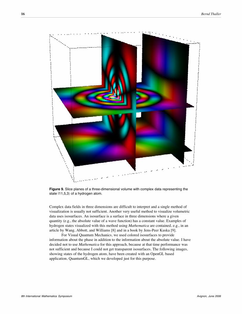
Figure 9. Slice planes of a three-dimensional volume with complex data representing the state |11,5,3\ of a hydrogen atom.

Complex data fields in three dimensions are difficult to interpret and a single method of visualization is usually not sufficient. Another very useful method to visualize volumetric data uses isosurfaces. An isosurface is a surface in three dimensions where a given quantity (e.g., the absolute value of a wave function) has a constant value. Examples of hydrogen states visualized with this method using Mathematica are contained, e.g., in an article by Wang, Abbott, and Williams [8] and in a book by Jens-Peer Kuska [9].

For Visual Quantum Mechanics, we used colored isosurfaces to provide information about the phase in addition to the information about the absolute value. I have decided not to use Mathematica for this approach, because at that time performance was not sufficient and because I could not get transparent isosurfaces. The following images, showing states of the hydrogen atom, have been created with an OpenGL based application, QuantumGL, which we developed just for this purpose.

16 Bernd Thaller


Figure 10. States of the hydrogen atom visualized with QuantumGL using (a) transparent, phase-colored isosurfaces, (b) an isosurface together with a phase-density plot, (c) layered transparent isosurfaces to create a fuzzy impression.



‡ Visualizations of higher-dimensional dataA source of difficulties for visualizations in quantum mechanics is the high dimensionality of the data. Even for single particles it becomes difficult to take into account, for example, the spin. The spin is usually described with two-component wave functions (spinors), that is, by two complex numbers at each point of space-time. In relativistic quantum mechanics, Dirac spinors are four dimensional, which amounts to the specification of eight real numbers at each point of space-time.

One possibility to visualize two-dimensional complex data is via ordinary vector field visualization. We can extract a three-dimensional vector field out of the spinor field in the following way. Let s× = Hs1, s2, s3L denote the Pauli matrices. For a given spinor y œ 2 , define the vector s× = Xy, s× y\, where X ÿ , ÿ\ is the scalar product in 2 . The length of the vector s× is the square of the norm of y, and the direction of s× gives the "spin-up"-direction of y. That means, y is the eigenvector belonging to the eigenvalue +1 of the matrix s× ÿ v× which represents the observable of the component of the spin in the direction of s×. In turn, the vector s× determines the spinor y uniquely up to a phase factor. Whenever the spinor y depends on the position, then also s× depends on the position, that is, the spinor defines a vector field which at every point gives the local spin-up direction of the particle (in quantum mechanics, the spin and the position are compatible observables that can be measured simultaneously).

We can now use common vector-field visualization techniques for the spin-vector field. One problem is that we want to visualize this three-dimensional vectorfield also if the spinor-valued function lives in only two space-dimensions. In two dimensions, 3D-vector fields cannot easily be visualized using flux lines. Attaching three-dimensional arrows to a two-dimensional surface often leads to images which are too cluttered to be informative, in particular, if the wave function has fine details.

But we can again make use of colors to represent vectors in three dimensions. Actually, the color manifold is three-dimensional and can be thus used to give a unique color to all vectors in three space. For the following image, we make use of all dimensions of the color manifold: The hue describes the direction in the x-y-plane, the lightness gives the z-component, and the saturation the absolute value. This color map for vectors uses the color circle in the x-y plane and blends these colors to white in the positive z-direction and to black in the negative z-direction. While the color map of the complex plane only made use of the colors that have the maximal saturation at a given lightness, we use here the saturation to encode the absolute value of a vector. The absolute value zero is mapped to saturation 0 (a 50 % gray) and large absolute values have full saturation.

The spin of a particle shows itself in the presence of a magnetic field. In an inhomogeneous field, particles with spin-up get accelerated in the direction of increasing field strength, while particles with spin-down get accelerated in the opposite direction (neglecting charge, for simplicity). This can be used to split an arbitrary spin state into its spin-up and spin-down components, and the corresponding type of experiments are called Stern-Gerlach experiments. The following sequence of images shows a particle passing through a Stern-Gerlach-like setup. A magnet, whose pole pieces are indicated at the top and the bottom of the images, provides an inhomogeneous magnetic field that increases in the vertical direction. This causes the particle, initially spin-polarized in the positive x-axis (therefore red) to split into a part that has spin spin-up (white) and a part that has spin-down (black). Note that the spin-up part of the wave packet gets accelerated in the direction of increasing field strength. When the particle enters the region between the magnets, there is an additional magnetic field inhomogeneity in the horizontal direction that causes the spin-up part to move faster than the spin-down part.

18 Bernd Thaller


Figure 11. Particle with spin-1/2 moving through a Stern-Gerlach apparatus and splitting into a spin-up part (white) and a spin-down part (black). Colors describe the local (position-dependent) direction of the particle's spin.

‡ References[1] B. Thaller, Visual Quantum Mechanics, Springer, New York 2000, ISBN 0-387-98929-3

[2] B. Thaller, Advanced Visual Quantum Mechanics, Springer, New York 2005, ISBN 0-387-20777-5

[3] B. Thaller, The Mathematica Journal 7(2), 163 (1998)

[4] M. Suzuki, Phys. Lett. A 146, 319 (1990), M. Liebmann, Diploma thesis, University of Graz 1999.

[5] Web resources for this article including whole movies and notebooks with source code may be found at http://vqm.uni-graz.at/articles/IMS06/.



[6] Handbook of Mathematical Functions, M. Abramowitz, I.A.Stegun, eds., Dover, New York, 9th printing 1970. See also http://www.convertit.com/Go/ConvertIt/Reference/AMS55.ASP

[7] M.V. Berry, J. Phys. A: Math. Gen 29, 6617 (1996)

[8] J.B. Wang, P.C. Abbott, J.F. Williams, Computers in Physics 10, 69 (1996)

[9] Jens-Peer Kuska, Mathematica und C in der modernen Theoretischen Physik, Springer-Verlag, Berlin Heidelberg New York 1997, ISBN 3-540-61489-3

‡ AuthorBernd ThallerInstitute for Mathematics and Scientific ComputingUniversity of GrazHeinrichstr. 36A-8010 [email protected]://math.uni-graz.at/thaller/

20 Bernd Thaller


visual quantum mechanics - home page of...

Documents