visual servoing: theory and applicationsrmal/books/1162_c15.pdf · chapter will be summarized in...

15Visual Servoing: Theory

and Applications

15.1 Introduction ................................................................... 15-115.2 Background..................................................................... 15-215.3 Servoing Structures ........................................................ 15-4

Position-Based Visual Servoing (PBVS) • Image-Based Visual Servoing (IBVS) • Hybrid Visual Servoing (HVS)

15.4 Examples....................................................................... 15-1515.5 Applications.................................................................. 15-1915.6 Summary ...................................................................... 15-20

15.1 Introduction

Conventional robotic systems are limited to operating in highly structured environments, and consider-able efforts must be expended to compensate for their limited accuracy. This is because conventionalrobotic manipulators operate on an open kinematic chain for placing and operating a tool (or end-effector) with respect to a workpiece. This is done by joint-to-joint kinematic transformations in orderto define the pose (position and orientation) of the endpoint with respect to a fixed-world coordinateframe. Similarly, the workpiece must be placed accurately with respect to the same coordinate frame.Any uncertainty or error about the pose of the endpoint or workpiece would lead to task failure. Potentialsources (such as gear backlashes, bending of the links, joints slippage, poor fixturing) would contributeto errors in the endpoint or workpiece poses. Therefore, considerable effort and cost are expended toovercome the above issues, for example, to design and manufacture special-purpose end-effectors, jigs,and fixtures. Consequently, due to the need for an accurate world model, the cost of changing the robottask would be quite high.

Alternatively, visual servoing provides direct measurements and control of the robot endpoint withrespect to the workpiece and hence does not rely on open-loop kinematic calculations. Visual servoingor vision-guided servoing is the use of vision in the feedback loop of the lowest level of a (usually robotic)system control with fast image processing to provide reactive behavior. The task of visual servoing forrobotic manipulators (or robotic visual servoing, RVS) is to control the pose of the robot’s end-effectorrelative to either a world coordinate frame or an object being manipulated, using real-time visual featuresextracted from the image. A camera can be fixed or mounted at the endpoint (eye-in-hand configuration).The advantages of robotic visual servoing can be summarized as follows:

1. It will relax the requirement for the exact specification of the workpiece pose. Therefore, it willreduce the costs associated with robot teaching and special-purpose fixtures. For example, it willallow operations on moving or randomly placed workpieces.

2. The requirement for exact positioning of the endpoint will be relaxed. Therefore, the robotoperation will not highly depend on stiffness and mechanical accuracy of the robot structure so

Farrokh Janabi-Sharifi

15-10-8493-1162-4/03/$0.00+$1.50© 2003 by CRC Press LLC

15

-2

Opto-Mechatronic Systems Handbook: Techniques and Applications

the robot mechanisms could be built lighter. This will lead to reduced cost of robot manufactureand operation, and decreased robot cycle time.

In summary, task specifications in a visual servoing framework would support robotic cells that arerelatively robust to many disturbing effects in unstructured environments and can adapt readily to minorchanges in the task or workpiece without needing to be reprogrammed.

One must distinguish visual servoing from traditional vision integration with robotic systems. Tradi-tional vision-based control systems [Shirai and Inoue, 1973] are typically look-and-move structures, wherevisual sensing and manipulation control are combined in an open-loop fashion. Therefore, image pro-cessing and robot control are independent with sequential operations. With look-and-move systems,image-processing times are long (in the order of 0.1 to 1 seconds), and the accuracy depends on theaccuracy of the vision system and the robot manipulator. In real visual servoing systems, the controlfeedback loop is closed around real-time image processing and measurements. The visual feedback loopoperates at a high sampling rate in the range of 100 Hz for direct control of the robot endpoint withrespect to an object and allows the operation of robot inner joint-servo loops at high sampling rates.Therefore, visual servoing systems provide improved accuracy and robustness to disturbing elements ofunstructured environments such as kinematic modeling errors and randomly positioned parts. Visualservoing is a truly mechatronic stream combining results from real-time image processing, kinematics,dynamics, control theory, real-time computation, and information technology.

The fundamentals of system modeling and image projection will be summarized in Section 15.2, thebasic classes of visual servoing systems will be presented in Section 15.3, simulation and experimentalexamples will be provided in Section 15.4, and the applications will be given in Section 15.5. Finally, thechapter will be summarized in Section 15.6.

15.2 Background

As shown in Figure 15.1, the coordinate frames that might be used for visual servoing include coordinateframes attached to the base (world frame), endpoint of the robot, camera, and object. For example, thelocation of an object viewed by the camera would be calculated with respect to the camera frame, or thelocation of the object might be determined with respect to the base frame. The homogeneous transformsbetween these frames are . Here is the homogenous transform from frame i toframe j, specified by a rotation matrix and translation vector . The camera is usually fixed withrespect to the endpoint or the world coordinate frame. Therefore, or could be obtained fromkinematic calibration tests. A common configuration is eye-in-hand configuration, where the camera ismounted at the endpoint, hence , i.e., coordinate frames E and C coincide. This configuration providesbetter viewing possibilities with less likelihood of viewing obstruction from the moving arm and target.

FIGURE 15.1 Relations between different coordinate frames: world, endpoint, camera, and object.

T T T TBE

EC

CO

BO, , , and T j

i

Rji Tj

i

TEC TB

C

T IEC =

Object frame{O}

Endpointframe{E}

Camera frame{C}

World orBase frame{B}

TRE

TBO

TEC

TCO

Visual Servoing: Theory and Applications

15

-3

For simplicity, in the remainder of this chapter, we will use frames E and C interchangeably, unless otherwisespecified.

Let T = (X, Y, Z)T denote the relative position vector of the object frame with respect to the cameraframe (Figure 16.2). We will also denote Q = (f , a, y )T as the relative orientation (or viewing direction)vector with roll, pitch, and yaw parameters, respectively. The pose W (position and orientation vector)of the object relative to the robot endpoint (or camera) will be then

(15.1)

We can define the relative task space t = SE3 = �3 ¥ SO3 as the set of all possible positions andorientations that could be attained by the end-effector. In general, however, we prefer to represent therelative pose by a 6D vector W Œ �6 of rather than by W Œ t .

The camera-projection model is shown in Figure 15.2. Each camera contains the projection of a three-dimensional scene in its two-dimensional (2D) image plane. Because depth information is lost, additionalinformation will be required to estimate the three-dimensional coordinates of a point P. This informationcould be obtained by multiple views of the object or by knowledge of the geometric relationship betweena set of feature points ei on the object. This information is obtained from image feature parameters.Although different image feature parameters are used in vision, in this chapter we will use the coordinatesof image feature points as image feature parameters. Good visual features depend on many parameterssuch as the feature’s radiometric properties, its visibility from many view points, and its ease of extractionwithout any ambiguity. Feature selection and planning for visual servoing is an important componentof any visual servoing system [Janabi-Sharifi and Wilson, 1997] and received a detailed discussion inanother chapter (see Chapter 14). In practice, hole and corner features are readily available in manyobjects and have proven to serve well for many visual servoing tasks [Feddema et al., 1991; Wilson et al.,2000]. Therefore, the rest of this chapter will focus on the use of hole and corner features.

A set of image feature parameters could be chosen to provide information about 6D relative posevectors at any instance of servoing. Therefore, image feature vector will be defined as s = [s1, s2, …, sk]

T

where each si Œ � is a bounded image feature parameter. Therefore, image feature parameter space (orshortly image space) S is defined as s Œ S �k. The projection will be a mapping denoted by

G :t Æ S. (15.2)

FIGURE 15.2 Projection of an object feature onto the image plane.

Pj

Pj

T

YO

XO

Object frame

Z O

ZC

XC

Camera frame

ii(xj , yj )

X i

Y i

Image frame

C

O

W T= =( , ) ( , , , , , ) .Q T TX Y Z f a y

Õ

15

-4


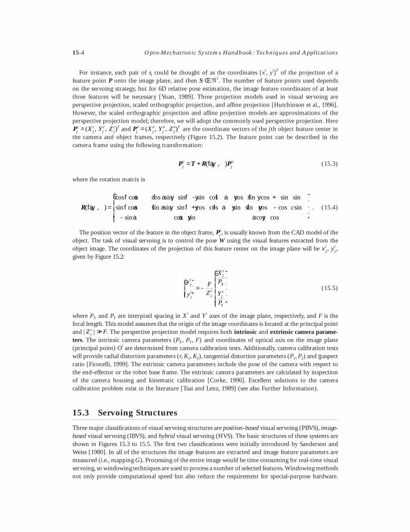
For instance, each pair of si could be thought of as the coordinates [xi, yi]T of the projection of afeature point P onto the image plane, and then S Œ �2. The number of feature points used dependson the servoing strategy, but for 6D relative pose estimation, the image feature coordinates of at leastthree features will be necessary [Yuan, 1989]. Three projection models used in visual servoing areperspective projection, scaled orthographic projection, and affine projection [Hutchinson et al., 1996].However, the scaled orthographic projection and affine projection models are approximations of theperspective projection model; therefore, we will adopt the commonly used perspective projection. Here

and are the coordinate vectors of the j th object feature center inthe camera and object frames, respectively (Figure 15.2). The feature point can be described in thecamera frame using the following transformation:

(15.3)

where the rotation matrix is

(15.4)

The position vector of the feature in the object frame, , is usually known from the CAD model of theobject. The task of visual servoing is to control the pose W using the visual features extracted from theobject image. The coordinates of the projection of this feature center on the image plane will be given by Figure 15.2:

(15.5)

where PX and PY are interpixel spacing in Xi and Yi axes of the image plane, respectively, and F is thefocal length. This model assumes that the origin of the image coordinates is located at the principal pointand . The perspective projection model requires both intrinsic and extrinsic camera parame-ters. The intrinsic camera parameters (PX , PY, F) and coordinates of optical axis on the image plane(principal point) Oi are determined from camera calibration tests. Additionally, camera calibration testswill provide radial distortion parameters (r, K1, K2), tangential distortion parameters (P1, P2) and g aspectratio [Ficocelli, 1999]. The extrinsic camera parameters include the pose of the camera with respect tothe end-effector or the robot base frame. The extrinsic camera parameters are calculated by inspectionof the camera housing and kinematic calibration [Corke, 1996]. Excellent solutions to the cameracalibration problem exist in the literature [Tsai and Lenz, 1989] (see also Further Information).

15.3 Servoing Structures

Three major classifications of visual servoing structures are position-based visual servoing (PBVS), image-based visual servoing (IBVS), and hybrid visual servoing (HVS). The basic structures of these systems areshown in Figures 15.3 to 15.5. The first two classifications were initially introduced by Sanderson andWeiss [1980]. In all of the structures the image features are extracted and image feature parameters aremeasured (i.e., mapping G). Processing of the entire image would be time consuming for real-time visualservoing, so windowing techniques are used to process a number of selected features. Windowing methodsnot only provide computational speed but also reduce the requirement for special-purpose hardware.

Pj

cjc

jc

jc TX Y Z= ( , , ) Pj

ojo

jo

jo TX Y Z= ( , , )

P T R Pj

cjo= + ( , , )f a y

R( , , )

cos cos cos sin sin sin cos cos sin cos sin sin

sin cos sin sin sin cos cos sin sin cos cos sin

sin cos sin cos cos

f a yf a f a y f y f a y f yf a f a y f y f a y f y

a a y a y=

- ++ -

-

È

Î

ÍÍÍ

˘

˚

˙˙˙

c .

Pjo

x yji

ji, ,

x

y

F

Z

X

P

Y

P

ji

ji

jc

jc

X

jc

Y

È

ÎÍÍ

˘

˚˙˙

= -

È

Î

ÍÍÍÍÍ

˘

˚

˙˙˙˙˙

| Z Fjc | >>

Visual Servoing: Theory and Applications

15

-5

Real-time feature extraction and robust image processing are crucial for successful visual servoing andwill be discussed in detail in another chapter (see Chapter 10). The feature- and window-selection blockin all of the shown structures uses current information about the status of the camera with respect tothe object and the models of the camera and environment to prescribe the next time-step features andthe locations of the windows associated with those selected features. Feature-selection and planning issuesare discussed in another chapter as well (see Chapter 14). In all of the structures, the visual servo controllers

FIGURE 15.3 Structure of position-based visual servoing (PBVS).

FIGURE 15.4 Structure of image-based visual servoing (IBVS).

OWE

_

+

Camera

object

Windows and FeaturesLocations

W~

W

Wd

Joint Servo Loops

Jointcontrollers

W E

W OCartesiancontroller

Poseestimation,G −1

Image featureextraction, G

Feature andwindowselection

Poweramplifiers

s

OWE_

+

Camera

object

s~sd


Joint Servo Loops

JointControllers

WE

WOFeaturespacecontroller



PowerAmplifiers

s

15

-6


determine set points for the robot joint-servo loops. Because almost any industrial robot has a joint–servointerface, this simplifies visual servo-control integration and portability. Therefore, the internal joint-level feedback loops are inherent to the robot controller, and visual servo-control systems do not needto deal with the complex dynamics and control of the robot joints.

In position-based control (Figure 15.3) the parameters extracted (s) are used with the models of cameraand object geometry to estimate the relative pose vector ( ) of the object with respect to the end-effector.The estimated pose is compared with the desired relative pose (Wd) to calculate the relative pose error( ). A Cartesian control law reduces the relative pose error, and the Cartesian control command istransformed to the joint-level commands for the joint-servo loops by appropriate kinematic transfor-mations.

In image-based control (Figure 15.4), the control of the robot is performed directly in the imageparameters space. The feature parameters vector extracted (s) is compared with the desired featureparameter vector (sd) to determine the feature-space error vector ( ). This error vector is used by afeature-space control law to generate a Cartesian or joint-level control command.

In hybrid control (Figure 15.5) such as 2-1/2D visual servoing, the pose estimation is partial anddetermines rotation parameters only. The control input is expressed partially in three-dimensionalCartesian space and in part in two-dimensional image space. An image-based control is used to controlthe camera translations, while the orientation vector is extracted and used to control the camerarotational degrees of freedom.

Each of the above strategies has its advantages and limitations. Several articles have reported thecomparison of the above strategies (see Further Information). In the next sections these methods willbe discussed, and simulation results will be provided to show their performance.

15.3.1 Position-Based Visual Servoing (PBVS)

The general structure of a PBVS is shown in Figure 15.3. A PBVS system operates in Cartesian space andallows the direct and natural specification of the desired relative trajectories in the Cartesian space, oftenused for robotic task specification. Also, by separating the pose-estimation problem from the control-design

FIGURE 15.5 Hybrid 2-1/2D visual servoing (HVS).

OWE

_

+

_

+sd

βu

Camera

object


Joint Servo Loops

Jointcontrollers

WE

WO

Rotationcontroller

Poseestimation,G −1



Poweramplifiers

s

Positioncontroller

u bd = 0

W

W

s

ub

Visual Servoing: Theory and Applications 15-7

problem, the control designer can take advantage of well-established robot Cartesian control algorithms.As will be shown in the Examples section, PBVS provides better response to large translational androtational camera motions than its counterpart IBVS. PBVS is free of the image singularities, localminima, and camera-retreat problems specific to IBVS. Under certain assumptions, the closed-loopstability of PBVS is robust with respect to bounded errors of the intrinsic camera-calibration and objectmodel. However, PBVS is more sensitive to camera and object model errors than IBVS. PBVS providesno mechanism for regulating the features in the image space. A feature-selection and switching mecha-nism would be necessary [Janabi-Sharifi and Wilson, 1997]. Because the relative pose must be estimatedonline, feedback and estimation are more time consuming than IBVS, with accuracy depending on thesystem-calibration parameters.

Pose estimation is a key issue in PBVS. Close-range photogrammetric techniques have been appliedto resolve pose estimation in real-time. The disadvantages of these techniques are their complexity andtheir dependency on the camera and object models. The task is to find (1) the relative pose of the objectrelative to the endpoint (W) using two-dimensional image coordinates of feature points (s) and (2)knowledge about the camera intrinsic parameters and the relationship between the observed featurepoints (usually from the CAD model of the object). It has been shown that at least three feature pointsare required to solve for the 6D pose vector [Yuan, 1989]. However, to obtain a unique solution at leastfour features will be needed.

The existing solutions for the pose-estimation problem can be divided into analytic and least-squaressolutions. For instance, unique analytical solutions exist for four coplanar, but not collinear, feature points.If intrinsic camera parameters need to be estimated, six or more feature points will be required for aunique solution (for further details see Further Information). Because the general least-squares solutionto pose estimation is a nonlinear optimization problem with no known closed-form solution, someresearchers have attempted iterative methods. These methods rely on refining the nominal pose estimationbased on real-time observations. For instance, Yuan [1989] reports a general iterative solution to poseestimation independent of the number of features or their distributions. To reduce the noise effect, somesort of smoothing or averaging is usually incorporated.

Extended Kalman filtering (EKF) provides an excellent iterative solution to pose estimation. Thisapproach has been successfully examined for 6D control of the robot endpoint using observations ofimage coordinates of 4 or more features [Wilson et al., 2000; Wang, 1992]. To adapt to the suddenmotions of the object an adaptive Kalman filter estimation has also been formulated recently for 6D poseestimation [Ficocelli and Janabi-Sharifi, 2001]. In comparison to many techniques Kalman-filter-basedsolutions are less sensitive to small measurement noise. An EKF-based approach also has the followingadvantages. First, it provides an optimal estimation of the relative pose vector by reducing image-parameter noise. Next, EKF-based state estimations improve solution impunity against the uniquenessproblem. Finally, the EKF-based approach provides feature-point locations in the image plane for thenext time-step. This allows only small window areas to be processed for image parameter measurementsand leads to significant reductions in image-processing time. Therefore, this section provides a briefdiscussion of EKF-based method that involves the following assumptions and conditions.

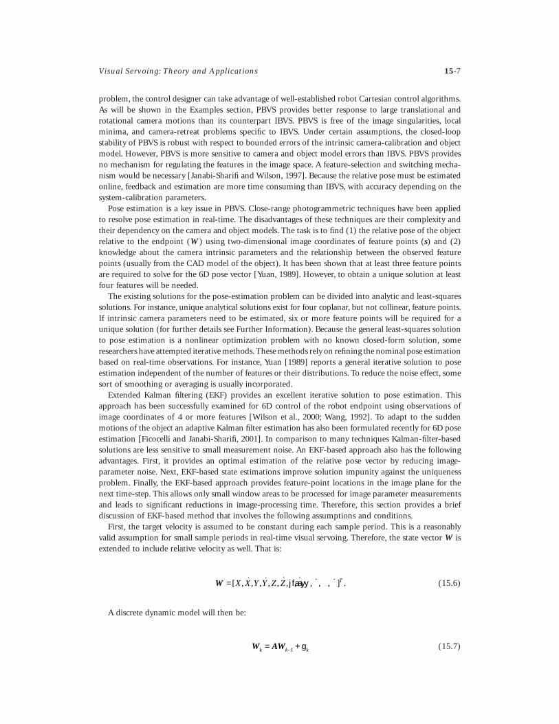
First, the target velocity is assumed to be constant during each sample period. This is a reasonablyvalid assumption for small sample periods in real-time visual servoing. Therefore, the state vector W isextended to include relative velocity as well. That is:

(15.6)

A discrete dynamic model will then be:

(15.7)

W =[ , ˙ , , ˙ , , ˙ , , ˙ , , ˙ , , ˙ ]X X Y Y Z Z Tj f a a y y .

W AWk k k= +- 1 g

15-8 Opto-Mechatronic Systems Handbook: Techniques and Applications

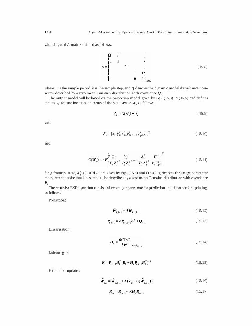
with diagonal A matrix defined as follows:

(15.8)

where T is the sample period, k is the sample step, and gk denotes the dynamic model disturbance noisevector described by a zero mean Gaussian distribution with covariance Qk.

The output model will be based on the projection model given by Eqs. (15.3) to (15.5) and definesthe image feature locations in terms of the state vector Wk as follows:

(15.9)

with

(15.10)

and

(15.11)

for p features. Here, are given by Eqs. (15.3) and (15.4). nk denotes the image parametermeasurement noise that is assumed to be described by a zero mean Gaussian distribution with covarianceRk.

The recursive EKF algorithm consists of two major parts, one for prediction and the other for updating,as follows.

Prediction:

(15.12)

(15.13)

Linearization:

(15.14)

Kalman gain:

(15.15)

Estimation updates:

(15.16)

(15.17)

A =

È

Î

ÍÍÍÍÍÍ

˘

˚

˙˙˙˙˙˙

¥

1

0 1

1

0 112 12

T

T

O

Zk kG= +( )W kn

Zk

i i i ipi

pi Tx y x y x y=[ , , , , , , ]1 1 2 2 K

G FX

P Z

Y

P Z

X

P Z

Y

P Zk

c

Xc

c

Yc

pc

X pc

pc

Y pc

T

( ) , , , ,W = -È

ÎÍÍ

˘

˚˙˙

1

1

1

1

L

X Y Zjc

jc

jc, , and

ˆ ˆ

, ,W AWk k k k- - -=1 1 1

P AP A Qk k k k

Tk, ,- - - -= +1 1 1 1

HW

W W Wk kk

G= ∂∂ = -

( )ˆ

, 1

K P H R H P H= +- -

-k k k

Tk k k k k

T, ,( )1 1

1

ˆ ˆ ( ( ˆ )), , ,W W K Z Wk k k k k k kG= + -- -1 1

P P KH Pk k k k k k k, , ,= -- -1 1


In the above equations, denotes the state predictions at time k based on measurements at timek – 1. Also, is the optimal state estimation at time k based on the measurements at time k. Pk,k- 1 andPk,k are state prediction error and state estimation error covariance matrices, respectively. K is the Kalmangain matrix. As mentioned above, the number of features used (p) should be above four to obtain aunique solution to 6D pose-vector estimation. However, inclusion of more features will improve theperformance of an EKF-based estimation, with a concomitant increase in cost for additional computa-tions. It has been shown that the inclusion of more than six features will not improve the performanceof EKF estimation significantly [Wang, 1992]. Also, the features need to be noncollinear and noncoplanarto provide good results. Consequently, 4 £ p £ 6 [Janabi-Sharifi and Wilson, 1997]. Further discussionon feature-selection issues is provided in Chapter 14.

The vision-based control system consists of fast inner joint-servo control loops. The slower outer loopis a visual servo control loop. The regulation aim in position-based control is to design a controller thatcomputes joint-angle changes to move the robot such that the relative pose reaches the desired relativepose in an acceptable manner. Therefore, control design for visual servo-control loops requires calculationof the error vector or the control command in joint space to provide the input commands to the joint-servo loops (Figure 15.3). For this purpose first the Euler angles Q must be converted to the total rotationangles q with respect to the endpoint frame [Wilson et al., 1996]. Assuming a slow-varying endpoint andobject frames within a sample period, the total rotation angles could be obtained from:

(15.18)

The orientation vector q and relative position vector T are compared with the input reference trajectorypoint to determine the endpoint relative-pose error in Cartesian space. Also, assuming slow-varyingmotion of the system without commanding any large abrupt changes, the endpoint relative position andorientation changes, e.g., error equations required for controlling the robot endpoint, are related to thejoint changes via:

(15.19)

One can regulate the joint level error Dq or Cartesian error DWE = [DTE , DqE]T. Different control lawshave been examined in the literature, e.g., PD control law to regulate Dq [Wilson, et al., 1996]. Note thatthe inner joint–servo control loops of common industrial robots operate at high sample rates, and forsmooth tracking performance high sample rates such as 60 Hz are usually expected from the visual servocontrol loop (i.e., outer loop). Due to the load of computations involved in PBVS, distributed computingarchitectures have been proposed to provide reasonable sample rates for the visual servo-control loop.For instance, Wilson et al. [1996] have reported a PBVS design and implementation using a transputer-based architecture with a coordinating PC. However, recent advances in microprocessor technology havemade high-speed PC-based implementation possible as well [Ficocelli and Janabi-Sharifi, 2001].

15.3.2 Image-Based Visual Servoing (IBVS)

In image-based visual servoing (Figure 15.4) the error signal and control command are calculated in theimage space. The task of the control is to minimize the error of the feature-parameter vector, given by

. An example of a visual task specified in the image space is shown in Figure 15.6. It shows theinitial and desired views of an object with five hole features. The advantage of IBVS is that it does notrequire full pose estimation and hence is computationally less involved than PBVS. Also, it is claimed

ˆ,Wk k- 1

ˆ,Wk k

qqqq

a f y f aa f y f a

f y a=

È

Î

ÍÍÍ

˘

˚

˙˙˙

ª- +

+-

È

Î

ÍÍÍ

˘

˚

˙˙˙

X

Y

Z

sin cos cos

cos sin cos

sin

DDD

q JR 0

0 R

TBE

E

ªÈ

ÎÍÍ

˘

˚˙˙

È

ÎÍÍ

˘

˚˙˙

- 1

BE

E

q

s s s= -d


that the positioning accuracy of IBVS is less sensitive to camera-calibration errors than PBVS. However,IBVS would lead to image singularities that might cause control instabilities. Another issue with IBVS isthe camera-retreat problem: For the commanded pure rotations around the optical axis, the camera oftenmoves away from the target in a normal direction and then returns. Moreover, the convergence of IBVSis ensured only in a small neighborhood of the desired camera pose. The domain of this neighborhoodis analytically impossible to determine [Chaumette, 1998]. The closed-loop stability is also robust withrespect to the errors of the camera-calibration and target model.

The goal of IBVS control is to find appropriate endpoint pose changes (or velocity) required tominimize error in the image space defined by (or its time rate). Because the robot control isusually in either Cartesian or joint space, the resultant control in image space must be converted intothe Cartesian- or joint-space error. The velocity (or differential changes) of the camera (or Dr) or itsrelative pose (or DW) can be related to the image feature velocities (or Ds) by a differential Jacobianmatrix, Ji , called image Jacobian. This matrix is also referred to as feature Jacobian matrix, featuresensitivity matrix, interaction matrix, or B matrix. Because we have assumed a hand-eye configuration,the endpoint frame (E) is coincident with the camera frame (C). Therefore, we will use endpoint andcamera frames or poses interchangeably. Then, Ji Œ �k¥m is a linear transformation from the tangentspace of t at W (or r) to the tangent space of S at s. Here, k and m are the dimensions of the image andtask spaces, respectively. Depending on the choice of endpoint pose representation, there are differentderivations for the image Jacobian matrix (see Further Information). For instance, if the relative pose ofthe object with respect to the endpoint is considered, we will have

(15.20)

where DWE is the differential change of the relative pose of the object defined in the endpoint (orcamera) frame. The corresponding image Jacobian matrix is given in Feddema et al. [1991]. It is alsopossible to relate the motion of a task frame to the motion of the feature points. In hand-eye configu-rations, it is preferable to define endpoint (or camera) motions with respect to the endpoint (or camera)frame. Therefore, DWE = [DTE, DqqqqE]T in Eq. (15.20) will imply the differential corrective motion of theendpoint with respect to the endpoint frame. The image Jacobian matrix for one feature can then bewritten as:

(15.21)

FIGURE 15.6 An example of a task specified in the image space with the initial and desired views.

s s s= -d

r

W s

D Ds J Wi E=

J i =- +

ÊËÁ

ˆ¯

- +ÊËÁ

ˆ¯

-

È

Î

ÍÍÍÍÍ

˘

˚

˙˙˙˙˙

F

P Z

x

Z

P

Fx y

F

P

P

Fx

P

Py

F

P Z

y

Z

F

P

P

Fy

P

Fx y

P

Px

Xc

i

cY i i

X

X i Y

X

i

Yc

i

cY

Y i X i i X

Y

i

0

0

2

2

.


Because several features (p) are used for 6D visual servoing, the image Jacobian matrix will have the form of:

(15.22)

where (Ji)k is a 2 ¥ 6 Jacobian matrix for each feature given by Eq. (15.21). Therefore, one can use Eqs.(15.20) and (15.22) to calculate endpoint differential motion (or its velocity) for a given change or errorexpressed in the image space. That is:

(15.23)

which assumes a nonsingular and square image Jacobian matrix. A control law can then be applied tomove the robot endpoint (or camera) toward the desired feature vector. The earliest and easiest controlapproach is resolved-rate motion control (RRMC), which uses a proportional control to warrantexponential convergence . Therefore:

(15.24)

where Kp is a diagonal gain matrix [Feddema et al., 1991] and u is the endpoint velocity screw. At thisstage a Cartesian-space controller can be applied. Because the control output will indicate endpointchanges (or velocity) with respect to the endpoint frame, transformations must be applied to calculatethe equivalent joint angles changes. Under the same assumptions as Eqs. (15.19), these calculations aregiven by:

(15.25)

RRMC is a simple and easy-to-implement method with a fast response time; however, it is not prone tosingularity and provides highly coupled translational and rotational motions of the camera. In additionto RRMC, other approaches to IBVS exist in the literature such as optimal control techniques, modelreference adaptive control (MRAC) methods, etc. (see Corke [1996]). Close examination of Eq. (15.25)reveals several problems with IBVS.

First, the image Jacobian matrix, given by Eqs. (15.21) and (15.22) depends on the depth Z c of thefeature. For a fixed camera, when the end-effector or the object held in the end-effector is tracked as theobject, this is not an issue because depth can be estimated using robot forward kinematics and camera-calibration data. For an eye-in-hand configuration, however, the depth or image Jacobian matrix mustbe estimated during servoing. Conventional estimation techniques can be applied to provide depthestimation; however, they increase computation time. Adaptive techniques for online depth estimationcan be applied, with limited success. Some proposals have been made to use an approximation to theimage Jacobian matrix using the value of the image Jacobian matrix or the desired features depthcomputed at the desired camera position. This solution avoids local minima and online updating of theimage Jacobian matrix. However, the image trajectories might be unpredictable and would leave imageboundaries. Further sources are provided in Further Information.

Second, the inverse of the image Jacobian matrix in Eq. (15.25) might not be square and full-rank(nonsingular). Therefore, pseudo-inverse solutions must be sought. Because p features are used for servoing,the dimension of the image space is k = 2p. Two possibilities exist when the image Jacobian matrix isfull rank, i.e., rank(ji) = min(2p, m) but 2p π m. If 2p < m, the pseudo-inverse Jacobian and least-squares

J

J

J

J

i

i

i

i

=

È

Î

ÍÍÍÍÍ

˘

˚

˙˙˙˙˙

( )

( )

( )

1

2

M

p

D DW J s W J sE i E i= =- -1 1, or ˙ ˙

˜ ˜s K sp=s Æ 0

u K J si= -p

1˜

Dq JR

RK J sP iª

È

ÎÍÍ

˘

˚˙˙

- -1 BE

BE

0

01 .


solution for (or DWE) will be:

(15.26)

(15.27)

with v as an arbitrary vector such that lies in the null space of Ji and allows endpoint motionswithout changes in the object features velocity. If 2p > m, the pseudo-inverse Jacobian and least-squaressolution for (or DWE) will be:

(15.28)

(15.29)

When the image Jacobian matrix is not full rank, the singularity problem must be dealt with. Smallvelocities of the image features near image singularities would lead to large endpoint velocities and resultin control instabilities and task failure. This problem might be treated by singular value decomposition(SVD) approaches or via damped least-squares inverse solutions.

Finally, IBVS introduces high couplings between translational and rotational motions of the camera,leading to a typical problem of camera retreat. This problem has been resolved by the hybrid 2-1/2Dapproach, which will be introduced in the next section. A simple strategy for resolving the camera-retreatproblem has also been introduced in Corke and Hutchinson [2000].

15.3.3 Hybrid Visual Servoing (HVS)

The advantages of both PBVS and IBVS are combined in recent hybrid approaches to visual servoing.Hybrid methods decouple control of certain degrees of freedom; for example, camera rotational degreescould be controlled by IBVS. These methods generally rely on the decomposition of an image Jacobianmatrix. A homography matrix is considered to relate camera configurations corresponding to the initialand desired images. This matrix can be computed by a set of corresponding points in the initial anddesired images. It is possible to decompose the homography matrix into rotational and translationalcomponents. Among hybrid approaches, 2-1/2D visual servoing is well established from an analytical pointof view. Therefore, the rest of this section will be devoted to the analysis and discussion of 2-1/2D visualservoing. Further details on other approaches can be found in the sources listed in Further Information.

In 2-1/2D visual servoing [Malis et al., 1999] the controls of camera rotational and translational degreesof freedom are decoupled. That is, the control input is expressed in part in three-dimensional Cartesianspace and in part in two-dimensional image space (Figure 15.5). IBVS is used to control the cameratranslational degrees of freedom while the orientation vector is extracted and controlled by a Cartesian-type controller. This approach provides several advantages. First, since camera rotation and translationcontrols are decoupled, the problem of camera retreat is solved. Second, 2-1/2D HVS is free of imagesingularities and local minima. Third, this method does not require full pose estimation, and it is evenpossible to release the requirement for the geometric model of the object. Fourth, Cartesian camera motionand image plane trajectory can be controlled simultaneously. Finally, this method can accommodate largetranslational and rotational camera motions. However, in comparison with PBVS and IBVS, 2-1/2D HVSintroduces some disadvantages that will be discussed after the introduction of the methodology, as follows.

For 2-1/2D HVS, first a pose estimation technique (e.g., scaled Euclidean reconstruction algorithm, SER[Malis et al., 1999]) is utilized to recover the relative pose between the current and the desired cameraframes, and then the vector is extracted. A rotation matrix R exists between the endpoint frame (or thecamera frame) denoted by E and the desired endpoint frame by E*. This matrix must reach identity matrixat the destination (Figure 15.7). In order to avoid workspace singularities, the rotation matrix will be

WE

˙ ˙ ( )W J s I J J viE = + -+ +

i i

J J J Ji iT

i iT+ -=( ) 1

( )I J J vi- +i

WE

˙ ˙W J sE = +i

J J J Ji iT

i iT+ -=( .) 1

ub

ub


represented by a vector (a unit vector of rotation axis) and a rotation angle b. For a 3 ¥ 3 rotation matrixwith elements rij, the vector could be obtained from:

(15.30)

and

(15.31)

where b = p can be detected through the estimation of b. Then the axis of rotation will be given bythe eigenvector associated with the eigenvalue of 1 of the rotation matrix. The endpoint velocity screwcan be related to the time derivative of the vector by a Jacobian matrix Lw, given by:

(15.32)

where S(.) is the skew-symmetric matrix associated with and I is an identity matrix. Malis et al. [1999]have shown that Lw is singularity free.

FIGURE 15.7 Modeling of the endpoint (or camera) displacement in a hand-eye configuration for 2-1/2D HVS.

uub

ubb

b p=---

È

Î

ÍÍÍ

˘

˚

˙˙˙

π1

2

32 23

13 31

21 12

sinc for

r r

r r

r r

sinc if 0

sin otherwise

bb

bb

==Ï

ÌÔ

ÓÔ

1

u

ub

L I u uwb b

b= - + -

Ê

Ë

ÁÁÁ

ˆ

¯

˜˜˜2

1

2

2S S( )

( )

( )sinc( )

sinc2

u


Next, a hybrid error vector (Figure 15.5) is defined as:

(15.33)

where are current and desired extended image parameter vectors, respectively. Consider areference feature point P with coordinates [X E, Y E, Z E]T with respect to the endpoint (or camera) frame.A supplementary normalized coordinate could be defined as z = logZ E with Z E as depth. Then, thenormalized and extended image vector will be:

(15.34)

Let represent the endpoint (or camera) velocity screw with respect to theendpoint frame. The velocity screw could be related to the hybrid error velocity by:

(15.35)

where

(15.36)

Here, L is the hybrid Jacobian matrix, with Lw given by Eq. (15.32),

(15.37)

and

(15.38)

Obviously, one can consider differential changes of the endpoint (or camera) pose and error insteadof their velocities. Note that Jacobian matrix L is singular only when ZE = 0, or = 0, or with b = ± 2p.These cases are exterior to the task space t , so the task space is free of image-induced singularities.

Finally, the exponential convergence of e Æ 0 is achieved by imposing a control law of the form:

(15.39)

e = --

È

ÎÍÍ

˘

˚˙˙

m m

ue e

*

b 0

m me e* and

me

i

i

i

E

E

E

E

E

x

y

z

X

Z

Y

Z

Z

=

È

Î

ÍÍÍ

˘

˚

˙˙˙

=

È

Î

ÍÍÍÍÍÍÍ

˘

˚

˙˙˙˙˙˙˙log

˙ [ , ] [ ˙ , ˙ ]W v TE E= ∫w qTE

WE e

˙˙

( ) ˙em

d

dt

LWe

E=È

ÎÍÍ

˘

˚˙˙

=ub

LL L

Lv v∫

-È

ÎÍ

˘

˚˙

( , )w

w0 .

Lv ∫

-

-

È

Î

ÍÍÍÍÍÍÍ

˘

˚

˙˙˙˙˙˙˙

10

01

0 01

2

2

Z

X

Z

Z

Y

Z

Z

E

E

E

E

E

E

E

L( , )

( )

v

i i i

i i i i

i i

x x y

y x y x

y xw ∫

- ++ - --

È

Î

ÍÍÍÍ

˘

˚

˙˙˙˙

1

1

0

2

2

.

1

Z E

e K e= - p


or

(15.40)

which could be simplified to:

(15.41)

Note that because , as proven by Malis et al. [1999]. Also, because L- 1 is anupper triangular matrix, the rotational control loop is decoupled from the translational one. Like Eq.(15.25), endpoint screw velocity can be expressed in terms of changes required in joint angles that willbe sent to the robot joint-servo loops for the execution.

Despite numerous advantages there are a few problems associated with 2-1/2D HVS. One of theproblems is the possibility of features leaving image boundaries. Some approaches have been proposedto treat this problem. Among them is the approach of Morel et al. who use a modified feature vector (seeFurther Information).

The second problem is related to noise sensitivity and computational expense of partial estimation inHVS. A scaled Euclidean reconstruction (SER) was originally used to estimate camera displacementbetween the current and desired relative poses [Malis et al., 1999]. This method does not require ageometric three-dimensional model of the object; however, SER uses recursive KF to extract the rotationmatrix from the homography matrix, while KF might be sensitive to camera calibration. Also, theestimation of the homography matrix requires more feature points, especially with noncoplanar objects.This is because when the object is noncoplanar, the estimation problem becomes nonlinear and willnecessitate at least eight features for homography matrix estimation at the video rate of 25 Hz. Anotherapproach would be to estimate the full pose of the object with respect to the camera by a fast and globallyconvergent method such as the orthogonal iteration algorithm (OI) of Lu and Hager (see FurtherInformation). Next, a homogeneous transformation could be applied to obtain camera-frame displace-ment. However, this would require a full three-dimensional model of the object.

Finally, the selection of reference feature point affects the performance of 2-1/2D HVS. A series ofexperiments would be required to select the best reference point for the improved performance.

15.4 Examples

Simulations and experiments were run to compare the performances of PBVS, IBVS, and HVS. AMATLABTM environment was created to simulate a five-degrees-of-freedom CRS Plus SRS-M1A robotwith an EG&G Reticon MC9000 CCD camera mounted at its endpoint (Figure 15.8). A 16-mm lens wasused. Simulation parameters are shown in Table 15.1. As shown in Figure 15.8, an object with fivenoncoplanar hole features was considered. The initial poses of the object and robot endpoint are alsoshown in Table 15.1.

A number of tests were run to investigate the effect of different parameters and compare the perfor-mances of different visual servoing methods. The control methods used for each strategy are EKF-basedpose estimation and PD control for PBVS, RMRC for IBVS, and 2-1/2D for HVS. The control gains weretuned by running a few simulations for stable and fast responses. The results are shown in Figures 15.9to 15.12. For simulations, an additive noise has been considered to represent more realistic situations.The general relative motion is shown in Figures 15.9 to 15.11 for PBVS, IBVS, and HVS. Initially, therobot endpoint is located above the object, i.e., in cm and rad, from Table 15.1.

W K L eE = - -p

1

˙ ( , )W KL L L

IeE p

v v v= --È

ÎÍ

˘

˚˙

- -1 1

0w

L Iw-

¥=13 3 Lw b b- =1u u

W E∞ = ∞ ∞ ∞[ , ,0 0 30, 0 , 0 , 0 ]T


TABLE 15.1 System Parameters for Simulations and Experiments

Parameter Value

Focal length, F 1.723 cmInterpixel spacings, Px , Py 0.006 cm/pixelNumber of pixels, Nx, Ny 128Features coordinates in frame {O} (5, 5, 0), (5, - 5, 0), (- 5, 5, 0), (- 5, - 5, 0), (0, 0, 3) cmInitial pose of object with respect to the base frame, [33.02, - 2.64, 0.38, - 0.0554, 0.0298, - 3.1409] (in cm and rad)Initial pose of the camera/endpoint with respect to the

base frame, [33.02, - 2.64, 30.38, - 0.0554, 0.0298, - 3.1409] (in cm and rad)

Initial relative depth, 30 cmOutput measurement covariance matrix of EKF, Rk diag[0.04, 0.01, 0.04, 0.01, 0.04, 0.01, 0.04, 0.01, 0.04, 0.01]

(pixel2)Disturbance noise covariance matrix of EKF, Qk diag[0, 0.8, 0, 0.8, 0, 0.8, 0, 0.8, 0, 0.001] in (cm/s)2 and

(deg/sec)2

FIGURE 15.8 Simulation environment with object model and its five features.

WB∞

WBE

Z EO


The figures show the relative pose errors for (X, Y, Z, qX, qY , qZ), i.e., the current relative pose minus thedesired relative pose, in the endpoint frame. The endpoint desired relative motion is indicated in thecaption of each figure. That corresponds to (3, - 3, - 5 cm, 0, 0.3, - 0.3 rad) translation and rotation alongand around the X, Y, and Z axes of the base frame, respectively, for the stationary object. Because the robothad five degrees of freedom, the commanded rotation about X axis was set to zero. Therefore, no errorof qX is shown. Also, errors in the image plane for the X and Y positions of five feature points (in pixels)are shown in Figures 15.9 and 15.11. Figure 15.12 shows the camera-retreat problem for IBVS. Only apure rotation around the optical Z axis of the camera was requested, but the camera moved away fromthe object and then returned. This problem was observed in neither PBVS nor HVS.

Some experiments were run for a different number of features and with different initial conditionsand relative poses. The joint couplings in the CRS robot had negative effects on the control responsesfor three-dimensional relative motions. The tests showed that a reasonably larger number of featurestended to improve the system response. The steady-state errors increased for all the methods with largecommanded relative motions. This applied particularly to the IBVS that used a nondecoupled imageJacobian matrix leading to coupled translational and rotational motions. When the commanded motionswere very close to the object, the steady-state error increased. Moreover, it was observed that PBVS andIBVS had almost the same response speed; however, HVS demonstrated a bit faster response than IBVSand PBVS, mainly due to the incorporation of the fast OI algorithm for estimation, instead of the SERused by Malis et al. [1999]. Choosing different reference points for HVS apparently had minimal effectson system performance. Finally, joint couplings of the CRS robot had considerable effect on the controlresponses for three-dimensional relative motions.

FIGURE 15.9 Simulation results for PBVS: desired relative pose of the object with respect to the endpoint frame:( . The relative pose errors are specified with respect to the endpoint frame {E}.

0 0.2 0.4 0.6 0.8 1−0.05

0

0.05

0.1

0.15

Time (s)

Err

or in

X (

m)

0 0.2 0.4 0.6 0.8 1−0.04

−0.02

0

0.02

Time (s)

Err

or in

Y (

m)

0 0.2 0.4 0.6 0.8 1−0.02

0

0.02

0.04

0.06

Time (s)

Err

or in

Z (

m)

0 0.2 0.4 0.6 0.8 1−0.4

−0.3

−0.2

−0.1

0

Time (s)

Err

or in

The

ta Y

(ra

d)

0 0.2 0.4 0.6 0.8 1−0.2

0

0.2

0.4

0.6

Time (s)

Err

or in

The

ta Z

(ra

d)

0 0.2 0.4 0.6 0.8 1−100

−50

0

50

100

Time (s)

Err

or in

Imag

e (p

ixel

)

- - -3 3 2, , 5 cm; 0, 0.3, 0.3 rad)


FIGURE 15.10 Simulation results for IBVS: desired relative pose of the object with respect to the endpoint frame:( . The relative pose errors are specified with respect to the endpoint frame {E}.

FIGURE 15.11 Simulation results for HVS: desired relative pose of the object with respect to the endpoint frame:( . The relative pose errors are specified with respect to the endpoint frame {E}.

0 0.2 0.4 0.6 0.8 1−0.05

0

0.05

0.1

0.15

Time (s)

Err

or in

X (

m)

0 0.2 0.4 0.6 0.8 1−0.04

−0.02

0

0.02

Time (s)

Err

or in

Y (

m)

0 0.2 0.4 0.6 0.8 1−0.02

0

0.02

0.04

0.06

Time (s)

Err

or in

Z (

m)

0 0.2 0.4 0.6 0.8 1−0.4

−0.3

−0.2

−0.1

0

Time (s)

Err

or in

The

ta Y

(ra

d)

0 0.2 0.4 0.6 0.8 1−0.2

0

0.2

0.4

0.6

Time (s)

Err

or in

The

ta Z

(ra

d)

0 0.2 0.4 0.6 0.8 1−100

−50

0

50

100

Time (s)

Err

or in

Imag

e (p

ixel

)

- - -3 3 2, , 5 cm; 0, 0.3, 0.3 rad)

0 0.5 1−0.05

0

0.05

0.1

0.15

Time (s)

Err

or in

X (

m)

0 0.5 1−0.04

−0.02

0

0.02

Time (s)

Err

or in

Y (

m)

0 0.5 1−0.02

0

0.02

0.04

0.06

Time (s)

Err

or in

Z (

m)

0 0.5 1−0.4

−0.3

−0.2

−0.1

0

Time (s)

Err

or in

The

ta Y

(ra

d)

0 0.5 1−0.1

0

0.1

0.2

0.3

Time (s)

Err

or in

The

ta Z

(ra

d)

0 0.5 1−100

−50

0

50

100

Time (s)

Err

or in

Imag

e (p

ixel

)

- - -3 3 2, , 5 cm; 0, 0.3, 0.3 rad)


15.5 Applications

Many applications of visual servoing have been limited to the laboratory and structured environments.For instance, many visual servoing systems use markers, structured light, and artificial objects withhigh-contrast features. Recent advances in opto-mechatronics technology have led to significantimprovements of visual servoing science and practice. A list of visual servoing achievements andapplications can be found in Corke [1996]. With the recent progress, it has been possible to designvisual servoing systems operating above 60 Hz, tracking and picking objects moving at 30 cm/s, applyingsealants at 40 cm/s, and guiding vehicles moving about 96 km/h. In summary, the current state of visualservoing technology has the potential to support robot operation in more realistic environments thantoday’s structured environments. This is particularly required in many emerging technologies for auton-omous systems.

Table 15.2 summarizes some of the demonstrated applications of visual servoing. However, many ofthese applications would not justify visual servoing applications, mainly due to the effectiveness of existingtraditional solutions. Commercial applications of visual servoing will occur with those applications thatthere are not substitute technologies. A good example is applications that require precise positioning,such as fixtureless assembly, within dynamic and uncertain environments.

Table 15.3 summarizes potential new applications of visual servoing. The main obstacle for thedevelopment of new applications is related to the robustness of vision in adapting to different and noisyenvironments. Research and development is underway to address vision and image-processing robustness.This topic is discussed further in Chapters 10 and 14.

FIGURE 15.12 Simulation results for IBVS: desired relative pose of the object with respect to the endpoint frame:( . The relative pose errors are specified with respect to the endpoint frame {E}.

0 0.2 0.4 0.6 0.8 1−2

0

2

4× 10

−3

Time (s)

Err

or in

X (

m)

0 0.2 0.4 0.6 0.8 1−10

−5

0

5× 10

−3

Time (s)

Err

or in

Y (

m)

0 0.2 0.4 0.6 0.8 1−0.01

0

0.01

0.02

0.03

Time (s)

Err

or in

Z (

m)

0 0.2 0.4 0.6 0.8 1−0.012

−0.011

−0.01

−0.009

−0.008

Time (s)

Err

or in

The

ta Y

(ra

d)

0 0.2 0.4 0.6 0.8 10

0.2

0.4

0.6

0.8

Time (s)

Err

or in

The

taZ

(ra

d)

0 0.2 0.4 0.6 0.8 1−50

0

50

Time (s)

Err

or in

Imag

e (p

ixel

)

0 0, , 0 cm; 0, 0, 4

rad)- p


15.6 Summary

Visual servoing, when compared with conventional techniques, offers many advantages for the controlof motion. In particular, visual servoing supports autonomous motion control systems without requiringexact specifications of poses for the object and tracker (e.g., robot endpoint). Also, visual servoing couldrelax the requirement for an exact object model. Visual servoing integration with robotic environmentshas significant implications such as fixtureless positioning, reduced robot training, and lower robot

TABLE 15.2 Demonstrated Applications of Visual Guidance and Servoing (Speeds Represent Those of the Objects; Numbers with Hz Denote Bandwidth of Visual Servoing System)

Application Investigators or Organizations, Date

Bolt insertion, picking moving parts from conveyor Rosen et al., 1976–1978 (SRI Int.)Picking parts from fast moving conveyor (30 cm/s) Zhang et al., 1990Tracking and grasping a toy train (25 cm/s, 60 Hz) Allen et al., 1991Visual-guided motion for following and grasping Hill and Park, 1979Three-dimensional vision-based grasping of moving

objects (61 Hz)Janabi-Sharifi and Wilson, 1998

Fruit picking Harrell et al., 1989Connector acquisition Mochizuki et al., 1987Weld seam tracking Clocksin et al., 1985Sealant application (40 cm/s, 4.5 Hz) Sawano et al., 1983Rocket-tracking camera with pan/tilt (60 Hz) Gilbert et al., 1980Planar micro-positioning (300 Hz) Webber and Hollis, 1988

(IBM Watson Research Center)Road vehicle guidance (96 Km/h) Dickmanns and Graefe, 1988Aircraft landing guidance Dickmanns and Schell, 1992Underwater robot control Negahdaripour and Fox, 1991Ping-pong bouncing Anderson, 1987Juggling Rizzi and Koditscek, 1991Inverted pendulum balancing Dickmanns and Graefe, 1988Labyrinth game Anderson et al., 1991Catching ball Bukowski et al., 1991Catching free-flying polyhedron Skofteland and Hirzinger, 1991Part mating (10 Hz) Geschke, 1981Aircraft refuelling Leahy et al., 1990Mating U.S. space shuttle connector Cyros, 1988Telerobotics Papanikolopoulos and Khosla, 1992Robot hand-eye coordination Hashimoto et al., 1989

TABLE 15.3 Potential Applications of Visual Guidance and Servoing

Potential Applications

Fixtureless assemblyAutomated machiningPC board inspection and solderingIC insertionRemote hazardous material handling (e.g., in nuclear

power plants)Weapons disassemblyRemote miningTextile manufacturingAutomated television and surveillance camera guidanceRemote surgerySatellite tracking and graspingPlanetary robotic missions


manufacturing costs and cycle time. In this chapter, the fundamentals of visual servoing were discussedand emphasis was placed on robotic visual servoing with eye-in-hand configurations. In particular, theemphasis was on the introduction of background theory and well-established methods of visual servoing.

An overview of the background related to visual servoing notations, coordinate transformations, imageprojection, and object kinematic modeling was given. Also, relevant issues of camera calibration werediscussed briefly.

The main structures of visual servoing, namely, position-based, image-based, and hybrid visual ser-voing structures, were presented. The basic and well-established control method for each structure wasgiven. The advantages and disadvantages of these control structures were compared.

Separation of the pose-estimation problem from the control-design problem, in position-based tech-niques, allows the control designer to take advantage of well-established robot Cartesian control algo-rithms. Also, position-based methods permit specification of the relative trajectories in a Cartesian spacethat provides natural expression of motion for many industrial environments, e.g., tracking and graspinga moving object on a conveyor. The interaction of image-based systems with moving objects, for example,has not been fully established. Position-based visual servoing provides no mechanism for regulatingfeatures in image space and, in order to keep the features in the field of view, must rely heavily on featureselection and switching mechanisms. Although both image-based and position-based methods demon-strate difficulties in executing large three-dimensional relative motions, image-based techniques show aresponse that is inferior to that of position-based methods, mainly due to the highly coupled translationaland rotational motions of the camera. Hybrid systems, such as the 2-1/2D method, show superiorresponse in comparison with their counterparts for long-range three-dimensional motions. This is mainlydue to the provision of decoupling between translation and rotation of the camera in hybrid systems.

Also, two major issues with image-based methods are the presence of image singularities and camera-retreat problems. These problems do not exist with position-based and hybrid methods. One disad-vantage of position-based methods over image-based and hybrid techniques is their sensitivity tocamera calibration and object model errors. Furthermore, the required computation time of theposition-based method is greater than that in image-based and hybrid methods. Hybrid methodsusually rely on the estimation of a homography matrix. This estimation might be computationallyexpensive and sensitive to camera calibrations. For instance, with noncoplanar objects and conventionalSER estimation of a homography matrix, more feature points might be required than those with othervisual servoing methods. However, with the recent advances in microprocessor technology, the com-putation-time should not pose any serious problems. In all of the techniques, the visual control loopmust be designed to provide higher bandwidth than that of robot position loops. Otherwise, the systemcontrol, like any other discrete feedback system with a delay, might become unstable by increasing theloop gain.

Simulations were done to demonstrate the performance of each servoing structure with the subscribedcontrol strategy. Moreover, the effects of different design parameters were studied and some conclusionswere drawn.

Finally, the demonstrated and potential applications of visual servoing techniques were summarized.Future research and development activities related to visual servoing were also highlighted.

Defining Terms

extrinsic camera parameters: Characteristics of the position and orientation of a camera, e.g., thehomogeneous transform between the camera and the base frame.

feature: Any scene property that can be mapped onto and measured in the image plane. Any structuralfeature that can be extracted from an image is called image feature and usually corresponds tothe projection of a physical feature of objects onto the image plane. Image features can be dividedinto region-based features, such as planes, areas, holes, and edge segment-based features, suchas corners and edges.


image feature parameter: Any quantity with real value that can be obtained from image features.Examples include coordinates of image points; the length and orientation of lines connectingpoints in an image, region area, centroid, and moments of projected areas; parameters of lines,curves, or regular regions such as circles and ellipses.

image Jacobian matrix: Relates the velocity (or differential changes) of the camera (or ) or itsrelative pose (or ) to the image feature velocities (or ). This matrix is also referred toas feature Jacobian matrix, feature sensitivity matrix, interaction matrix, or B matrix.

intrinsic parameters of the camera: Inner characteristics of the camera and sensor, such as focal lengthand radial and tangential distortion parameters, and the coordinates of the principal point, wherethe optical axis intersects the image plane.

visual servoing (vision-guided servoing): The use of vision in the feedback loop of the lowest level ofa (usually robotic) system control with fast image processing to provide reactive behavior. Thetask of visual servoing for robotic manipulators (or robotic visual servoing, RVS) is to controlthe pose of the robot’s end-effector relative to either a world coordinate frame or an object beingmanipulated, using real-time visual features extracted from the image. The camera can be fixedor mounted at the endpoint (eye-in-hand configuration).

Acknowledgments

This work was supported by the Natural Sciences and Engineering Research Council of Canada (NSERC)through Research Grant #203060-98. I would also like to thank my Ph.D. student Lingfeng Deng for hisassistance in the preparation of the simulation results.

References

Chaumette, F., Potential problems of stability and convergence in image-based and position-based visualservoing, The Confluence of Vision and Control, Vol. 237 of Lecture Notes in Control and InformationSciences, Springer-Verlag, New York, 1998, pp. 66–78.

Corke, P. I., Visual Control of Robots: High Performance Visual Servoing, Research Studies, Ltd., Somerset,England, 1996.

Corke, P. I. and Hutchnison, S. A., A new hybrid image-based visual servo-control scheme, Proc. IEEEInt. Conf. Decision and Control, 2000, pp. 2521–2526.

Feddema, J. T., Lee, C. S. G., and Mitchell, O. R., Weighted selection of image features for resolved ratevisual feedback control, IEEE Trans. Robot. Automat., 7(1), 31–47, 1991.

Ficocelli, M., Camera Calibration: Intrinsic Parameters, Technical Report TR-1999-12-17-01, Roboticsand Manufacturing Automation Laboratory, Ryerson University, Toronto, 1999.

Ficocelli, M. and Janabi-Sharifi, F., Adaptive Filtering for Pose Estimation in Visual Servoing, IEEE/RSJInt. Conf. on Intelligent Robots and Systems, IROS 2001, Maui, Hawaii, 2001, pp. 19–24.

Hutchinson, S., Hager, G., and Corke, P. I., A tutorial on visual servoing, IEEE Trans. Robot. Automat.,12(5), 651–670, 1996.

Janabi-Sharifi, F. and Wilson, W. J., Automatic selection of image features for visual servoing, IEEE Trans.Robot. Automat., 13(6), 890–903, 1997.

Malis, E., Chaumette, F., and Boudet, S., 2-1/2D visual servoing, IEEE Trans. Robot. Automat., 15(2),238–250, 1999.

Sanderson, A. C. and Weiss, L. E., Image-based visual servo control using relational graph error signals,Proc. IEEE, 1980, pp. 1074–1077.

Shirai, Y. and Inoue, H., Guiding a robot by visual feedback in assembling tasks, Pattern Recognition, 5,99–108, 1973.

Tsai, R. and Lenz, R., A new technique for fully autonomous and efficient three-dimensional robotichand/eye calibration, IEEE Trans. Robot. Automat., 5(3), 345–358, 1989.

r DrW DW s Ds


Wang, J., Optimal Estimation of Three-Dimensional Relative Position and Orientation for Robot Control,M.A.Sc. dissertation, Dept. of Electrical and Computer Engineering, University of Waterloo, Waterloo,Canada, 1992.

Wilson, W. J., Williams Hulls, C. C., and Bell, G. S., Relative end-effector control using cartesian position-based visual servoing, IEEE Trans. Robot. Automat., 12(5), 684–696, 1996.

Wilson, W. J., Williams-Hulls, C. C., and Janabi-Sharifi, F., Robust image processing and position-basedvisual servoing, in Robust Vision for Vision-Based Control of Motion, Vincze, M. and Hager, G. D.,Eds., IEEE Press, New York, 2000, pp. 163–201.

Yuan, J. S. C., A general photogrammetric method for determining object position and orientation, IEEETrans. Robot. Automat., 5(2), 129–142, 1989.

For Further Information

A good collection of articles on visual servoing can be found in IEEE Trans. Robot. Automat., 12(5), 1996.This issue includes an excellent tutorial on visual servoing. A good reference book is Visual Control ofRobots: High Performance Visual Servoing by P. I. Corke (Research Studies, Ltd., Somerset, England, 1996),encompassing both theoretical and practical aspects related to visual servoing of robotic manipulators.Robust Vision for Vision-Based Control of Motion, edited by M. Vincze and G. D. Hager (IEEE Press, NewYork, 2000) provides recent advances in the development of robust vision for visual servo-controlledsystems. The articles span issues including object modeling, feature extraction, feature selection, sensordata fusion, and visual tracking. Robot Vision, by B. K. Horn (McGraw-Hill, New York, 1986) is acomprehensive introductory book for the application of machine vision in robotics.

Proceedings of IEEE International Conference on Robotics and Automation, IEEE Robotics and AutomationMagazine, Proceedings of IEEE/RSJ International Conference on Intelligent Robots and Systems, IEEE Trans-actions on Robotics and Automation, and IEEE Transactions on Systems, Man, and Cybernetics documentthe latest developments in visual servoing.

Several articles have compared the performances of basic visual servoing methods. Among them are“Potential Problems of Stability and Convergence in Image-Based and Position-Based Visual Servoing,”by F. Chaumette, in The Confluence of Vision and Control, Vol. 237 of Lecture Notes in Control andInformation Sciences (Springer-Verlag, New York, 1998, pp. 66–78), and “Stability and Robustness ofVisual Servoing Methods,” by L. Deng, F. Janabi-Sharifi, and W. J. Wilson, in Proc. IEEE Int. Conf. Robot.Automat. (Washington, D.C., May 2002).

Good articles for camera calibration include the one by Tsai and Lenz [1989] and also “Hand-EyeCalibration,” by R. Horaud and F. Dornaike, in International Journal of Robotics Research, 14(3), 195–210,1995. Implementation details can also be found in Corke [1996].

Articles for analytical pose estimation include the following. For pose estimation using four coplanarbut not collinear feature points, see “Random Sample Consensus: A Paradigm for Model Fitting withApplications to Image Analysis and Automated Cartography,” by M. A. Fischler and R. C. Bolles, inComm. ACM, 24, 381–395, 1981. If camera intrinsic parameters need to be estimated, six or more featurepoints will be required for a unique solution. This is shown in “Decomposition of TransformationMatrices for Robot Vision,” by S. Ganapathy, in Pattern Recog. Lett. 401–412, 1989. See also “Analysis andSolutions of the Three Point Perspective Pose Estimation Problem,” by R. M. Haralick, C. Lee, K.Ottenberg, and M. Nolle, in Proc. IEEE Conf. Comp. Vision, Pattern. Recog., pp. 592–598, 1991, and “AnAnalytic Solution for the Perspective 4-Point Problem,” by R. Horaud, B. Canio, and O. Leboullenx,Computer Vision Graphics, Image Process., no. 1, 33–44, 1989.

The articles for the least-squares solutions in pose estimation include an article by S. Ganapathy [1989],mentioned above, and “Determination of Camera Location from 2-D to 3-D Line and Point Correspon-dences,” by Y. Liu, T. S. Huang, and O. D. Faugeras, in IEEE Trans. Pat. Anal. Machine Intell., no. 1, 28–37,1990. Also, “Constrained Pose Refinement of Parametric Objects,” by R. Goldberg, in Int. J. Comput.Vision, no. 2, 181–211, 1994. A fast and globally convergent orthogonal iteration (OI) algorithm is


introduced in “Fast and Globally Convergent Pose Estimation from Video Images,” by C. P. Lu and G. D.Hager, in IEEE Trans. Patt. Analysis and Machine Intell., 22(6), 610–622, June 2000.

The following references provide solutions to online estimation of depth information and imageJacobian matrix for IBVS. “Manipulator Control with Image-Based Visual Servo,” by K. Hashimoto,T. Kimoto, T. Ebine, and H. Kimura, in Proc. IEEE Int.Conf. Robot. Automat., Piscataway, NJ, 1991, pp.2267–2272 provides an explicit depth estimation based on the feature analysis. An adaptive control-basedmethod for depth estimation is provided in “Controlled Active Vision,” by N. P. Papanikolopoulos, Ph.D.dissertation, Dept. of Electrical and Computer Engineering, Carnegie Mellon University, 1992. It is alsoproposed to use an approximation to the value of the image Jacobian matrix computed at the desiredcamera position, in “A New Approach to Visual Servoing in Robotics,” by B. Espiau, F. Chaumette, andP. Rives, in IEEE Trans. Robot. Automat., 8(3), 313–326, 1992.

There are different image Jacobian derived in the literature. The following sources could be studiedfor further details: [Feddema et al., 1991], and “Vision Resolvability for Visually Servoed Manipulation,’’by B. Nelson, and P. K. Khosla, in Journal of Robotic Systems, 13(2), 75–93, 1996. Also see “ControlledActive Vision,” by N. P. Papanikolopoulos, Ph.D. dissertation, Dept. of Electrical and Computer Engineering,Carnegie Mellon University, 1992.

Other forms of image Jacobian matrices have been derived using geometrical entities, such as spheresand lines, are also available in: “A New Approach to Visual Servoing in Robotics,” by B. Espiau et al.,mentioned above. Also see Malis et al. [1999] for Jacobian matrix for 2-1/2D servoing.

In addition to Malis et al. [1999], the following papers are good resources for the study of HVS. Forinstance, the following paper proposes a solution for features leaving field-of-view in 2-1/2D HVS:“Explicit Incorporation of 2-D Constraints in Vision-Based Control of Robot Manipulators,” by G. Morel,T. Liebezeit, J. Szewczyk, S. Boudet, and J. Pot, in Experimental Robotics VI, P. I. Corke and J. Trevelyan,Eds., Vol. 250, Springer-Verlag, 2000, pp. 99–108. The following article proposes to compute translationalvelocity instead of rotational one for HVS: “Optimal Motion Control for Image-Based Visual Servoingby Decoupling Translation and Rotation,” by K. Deguchi, in Proc. IEEE Int. Conf. Intel. Robotics andSystems, 1998, pp. 705–711. Also see Corke and Hutchinson [2000] for a new partitioning of cameradegrees of freedom. That includes separating optical axis z and computing z-axis velocity using two newimage features.

The following sources are useful for the study of homography matrix and its decomposition used inHVS: Three-Dimensional Computer Vision, by O. Faugeras, MIT Press, Cambridge, MA, 1993, and“Motion and Structure from Motion in a Piecewise Planar Environment,” in Int. J. Pattern Recogn.Artificial Intelligence, 2, 485–508, 1988.

The following sources cover the applications developed using VS techniques: Corke [1996] and “VisualServoing: A Technology in Search of an Application,” by J. T. Feddema, in Proc. IEEE Int. Conf. Robot.Automat: Workshop on Visual Servoing: Achievements, Applications, and Open Problems, San Diego, CA,1994.

visual servoing: theory and applicationsrmal/books/1162_c15.pdf · chapter will be summarized in...

Documents