visual simulation of forest regrowth under different ... · pdf filevisual simulation of...

Visual Simulation of Forest Regrowth Under Different

Harvest Options

Ian D. BISHOP, Gillian FASKEN, Rebecca FORD, John HICKEY, Daniel LOITERTON

and Kathryn WILLIAMS

1 Introduction

Forest harvesting is a controversial topic in Australia. The Australian public has a special

affection for the native Eucalpytus forest and the animals it supports. The practice of

clearfelling, followed by high temperature burning and aerial sowing of eucalypt seeds

(clearfell, burn and sow- CBS) is the most commonly used approach for wood production

in tall wet eucalypt forest in south-east Australia (FLORENCE, 1996). This creates a short-

term scene of apparent devastation within a harvest block – locally called a coupe – which

is seen by some members of the public as a ruthless approach, insensitive to the values of

sustainability, wildlife habitat and aesthetics. The public and private forest management

agencies, on the other hand, see the practice as both the most efficient – in terms of cost of

timber removal – and also among the safest and most environmentally appropriate

practices. This division of opinion has led to vociferous public debate and also physical

resistance to forest harvest as people have chained themselves to trees, made temporary

homes high in the branches and sabotaged forest harvesting equipment.

Sensitive to the controversy, Forestry Tasmania has established a silvicultural systems trial

(HICKEY ET AL. 2001) within the Warra Long Term Ecological Research (LTER) site to

undertake scientific research into the consequences of alternative forest management

practices. The Warra LTER site (Brown et al. 2001) is an area of wet eucalypt forest with a

very dense understorey. The dominant species, and main timber tree, is the stringybark

(Eucalyptus obliqua). The major understorey species are dogwood (Pomaderris apetala),

myrtle (Nothofagus cunninghamii) and silver wattle (Acacia dealbata). Several other

species occur in smaller numbers but are economically important: e.g. leatherwood

(Eucryphia lucida) for bee keepers, celery top pine (Phyllocladus aspleniifolius) for boat

builders and joiners.

From 1998-2003, sections of forest have been harvested to prescribed patterns and the

distribution of seed fall, germination and regrowth monitored. The harvest and regeneration

treatments being rigorously assessed are:

• Clearfell, burn and sow: this is the traditional approach described above. The area

cleared is typically about 60 ha, the burn is hot.

• Dispersed retention: a percentage of individual eucalypt trees are retained for a

full rotation for fauna habitat and natural seed supply. The slash is partially-

cleared using a low intensity burn.

• Aggregated retention: islands of undisturbed forest are retained for a full rotation

for habitat, seed supply (all species) and aesthetics. A low intensity burn is used.

I. Bishop, G. Fasken, R. Ford, J. Hickey, D. Loiterton and K. Williams 2

• Strip harvest: harvesting is restricted to 80 m wide alternate strips, with strips of

undisturbed forest retained for half the rotation for habitat and seed supply (all

species). A low intensity burn is used.

• Small group selection (SGS): individual or very small groups of trees are felled

and removed leaving the remaining forest largely intact. There is no burning or

artificial seeding.

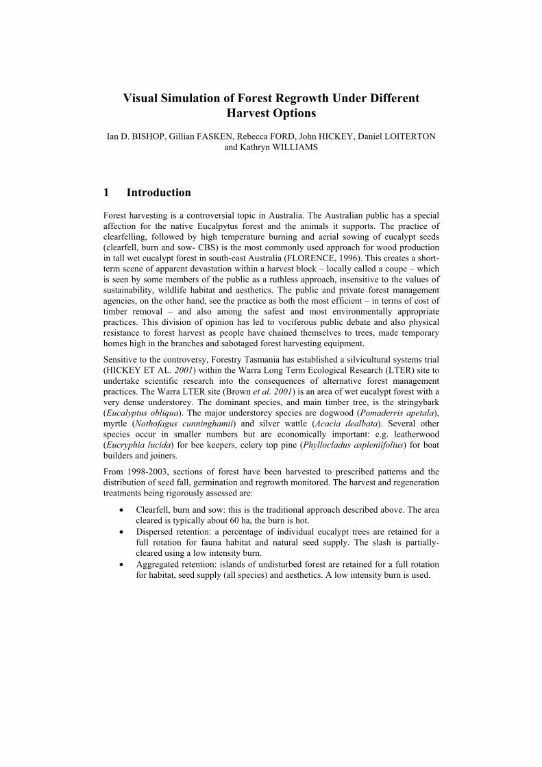
In order to present the public with an understanding of the full harvest and management

sequence – as distinct from the emotive view of a burnt scar – we are creating animation

sequences covering 200 years of forest life. This is typically two harvest cycles. It was also

recognized that fire is a natural and frequent component of the life of the forest regardless

of the extent of human intervention and that in any 200 year period at least one destructive

wild fire could be expected. The site for the simulations is a Forestry Tasmania harvest

coupe called AR033a (Fig. 1) which had recently been harvested using the clearfell, burn

and sow system (CBS). This was chosen as the base within which other harvest systems

would be simulated.

Fig 1: Coupe AR033a. This 51 ha coupe is just outside the Warra experimental site but

has the same forest type and was burnt and sown in autumn 2002.

Computer based forest simulation has a long history dating from MYKLESTADT AND

WAGER (1977). Their distorted square terrain representation and arrow-head trees lasted

as the dominant approach for almost a decade but has gradually been replaced by

increasingly sophisticated procedures for rendering both terrain and vegetation. Today the

terrain is typically draped with aerial photographs or generic textures to represent the

known land uses. Trees are either fully modeled in three-dimensions or based on detailed

Visual Simualation of Forest Regrowth under Different Harvest Options 3

images texture-mapped onto planar surfaces (either fixed intersecting planes or rotating

billboards). The several options are more fully described in MUHAR (2001).

The degree to which computer simulations match the real world has been tested in a

number of studies (e.g. BERGEN ET AL., 1995). KARJALAINEN AND TYRVAINEN

(2002), working specifically in the forest context, described criteria for creating appropriate

visualizations. The creation of a realistic image requires technical accuracy: colours, shapes

and textures that are suitable for the conditions being simulated; high resolution; and a

viewpoint that creates the correct perspective. In addition there must be integrity with the

spatial data that defines the forest area: precision in location, species proportions, growth

rates and densities. In their assessment of different types of visualisations in landscape

preference research, they found that although on-site visits met all the criteria, there was

little control over other variables such as weather and conditions, which can influence a

person's judgement. Having a simulation enabled those variables to be controlled. As well

as added control, “visualisation methods can provide perspectives and representations of

both temporal and spatial features that may be difficult to carry out in real on-site

experience, possibly producing more insightful evaluations than on-site visits can provide.”

(p18)

2 Preliminary Simulation and Assessment

The first task was to determine which elements of the forest environment are the most

important to simulate, and what were the salient features of these elements that required

accurate potrayal. These questions were examined in a field study, in which people from a

range of interest groups assessed preliminary simulations in a number of ways. First,

simulations were created using simplified versions of the procedures described in detail

below and an initial set of still images was produced. The forest elements included in these

simulations were based on researchers observations of the site and on advice from

professional foresters. These images corresponded to a limited range of conditions

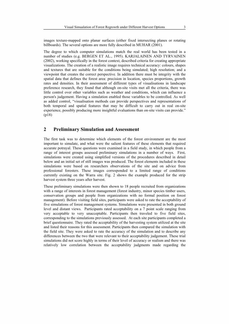
currently existing on the Warra site. Fig. 2 shows the example produced for the strip

harvest system three years after harvest.

These preliminary simulations were then shown to 18 people recruited from organizations

with a range of interests in forest management (forest industry, minor species timber users,

conservation groups and people from organizations with no formal position on forest

management). Before visiting field sites, participants were asked to rate the acceptability of

five simulations of forest management systems. Simulations were presented in both ground

level and distant views. Participants rated acceptability on a 7 point scale ranging from

very acceptable to very unacceptable. Participants then traveled to five field sites,

corresponding to the simulations previously assessed. At each site participants completed a

brief questionnaire. They rated the acceptability of the harvesting system utilized at the site

and listed their reasons for this assessment. Participants then compared the simulation with

the field site. They were asked to rate the accuracy of the simulation and to describe any

differences between the two that were relevant to their acceptability judgement. These trial

simulations did not score highly in terms of their level of accuracy or realism and there was

relatively low correlation between the acceptability judgments made regarding the


simulations and the field sites. Participant descriptions of differences between the

simulation and the field site highlighted a number of areas for improvement of the

preliminary simulations. These issues and some of the lessons drawn from them are

summarised in Table 1.

(a) distant view superimposed on aerial

photograph

(b) ground level view

Fig 2: Preliminary simulations of the strip harvest system three years after harvest.

3 Realistic Simulation Process

Based on our initial experiences and the on-site assessments and commentary we began a

new round of simulation development taking care to address the specific concerns raised.

The stages of the process are described in detail below. A key element in the process,

which shaped to a considerable extent the stages which precede it, was the selection of the

rendering software. Several packages, which could potentially assist with the model

development and rendering process, were available. These included 3Dstudio Max, Bryce

and the public domain programs Forester (www.dartnall.f9.co.uk/forester) and VTP

(vterrain.org). None of these, however, gave us the level of control we needed to generate a

time series of images in which:


Table 1: Some of the visual features of the simulation mentioned by at least 25% of the

focus group (N=18), the qualities of the simulation features which are relevant

and the possible enhancements to the simulation process.

Visual feature Qualities of the feature Possible Enhancements

Simulation has less

impact than field site

On-site effect more

powerful

Picture can’t convey

sound

Project simulations to a large size so they fill

the field of view –requires good resolution

Can include sound in simulations – but which

sound?

Eucalypt regeneration

poorer in the field than

in simulations

Quantity of

regeneration and

distribution across the

site

Size, health, form and

uniformity of

regenerating trees

Models used to simulate tree height and

density may have been optimistic and should

be reviewed

Tree photographs for use in simulations need

to be representative of native forest

regeneration

Understorey species

dominate regeneration

in field but not visible

in simulations

Regeneration consists

mostly of sedges and

other understorey plants

Focus on simulating visually distinctive

species, for example cutting grass (Gahnia

grandis) – information is needed on its height

and density for different harvest systems

Logging residue detail

not visible in

simulations

Stump and log size

Amount and quality of

waste logs and standing

trees

Extent to which residue

has been burnt

Need information about:

• size of logs, stumps and remaining trees

• no per ha and their distribution

• proportion of the surface which is

blackened for each harvest system

• trees were randomly located but remained in the same location at the next time step.

• several different textures were available for each species and were randomly

allocated to individuals of that species.

• the textures could be changed at a specific age corresponding to a change in the

growth habit of the species.

• the crossed-planes upon which the textures were pasted were randomly rotated – but

retained that rotation as they grew.

• within each age class a level of height variation was randomly distributed.

To achieve complete control over the rendered model we chose to use the public domain

renderer POV-Ray. This is wholly controlled by text files which describe the scene in the


POV-Ray modeling language. We then developed a Visual Basic program (described in

more detail below) to generate the text files.

3.1 Determination of Forest Species Mix and Distribution Over Terrain

Existing data from previous vegetation surveys were used to generate tables of likely

species density at selected ages (1, 3 10, 25 and 89 years). Growth formulae have also

been developed for the most common species and used to compute the heights of the plants

at the key ages (Table 2).

Table 2: Height and density estimates at different ages for the clearfell, burn and sow

condition. Similar tables exist for the other harvest systems.

Age Eucalypt Acacia Myrtle

Height (m) Density

(stms/ha)

Height (m) Density

(stms/ha)

Height (m) Density

(stms/ha)

3

4.5

3000 4.3

10000

0.3

100

10 12.1 1000 10.3 8000 1 100

25 23.5 500 14.1 3000 2.5 100

89 44.1 250 26.5 500 9 200

The process of allocating individuals of each species to a location in the terrain began by

creation, using a VB program, of a very large number of random points at coordinates with

the minimum bounding rectangle of the chosen coupe. These points were imported, as a

text file, into ArcView. For each harvest system, areas of retained trees were defined by

Forestry Tasmania officers. These boundaries were digitized into ArcView and then used

to cull the random points to leave the new growth points. A height for each point was then

allocated by interpolation from the DEM.

3.2 Development of Individual Trees

Although in this project we aim to produce effective animations of growth rather than an

interactive environment, we still decided to use the simpler texture mapping approach to

tree modeling. This was because:

• the species found in the Tasmania wet forest are very much under-represented in

the public domain or commercial 3D tree model libraries; and

• the presence of hundreds of thousands of trees with each modeled as several

hundred polygons would have made rendering too slow to complete our

animations in a realistic time frame.

Therefore, models of the various tree species at each different age were produced using the

simple billboard method, with textures displayed on two planes at right angles. The first


step in this process was to take a large number of high-resolution digital photos of each

required species at varying ages. For the best results, a clear blue background is required so

that the green leaves of the tree can be easily distinguished from whatever is beyond it. For

larger trees this was simply a case of finding examples that were out in the open with a

clear blue sky behind them (morning or afternoon sun directly behind the camera gives the

best results). For smaller plants, we either cut the stem off at the base and held it up to the

sky, or held a blue tarpaulin behind it while the photo was taken.

The digital photographs were then opened in Adobe Photoshop where a number of

different techniques were used, depending on the photo’s quality, to delete all of the pixels

which were not a part of the tree. The simplest way of doing this is to delete all pixels

within a certain colour range (ie. all shades of blue). Where the tree was in front of other

vegetation or ground, an area selection tool was used to carefully trace around the tree’s

foliage. With either of these methods, there are always some background pixels that

remain, giving the tree an undesirable blue or white outline. However, by adjusting the hue

and saturation of all blue and cyan pixels until they matched the colour of the tree, we were

able to combat this effect. The process is illustrated in Fig. 3.

Fig 3: Texture creation process.

Once all the textures of a given species were completed, the red, blue, and green

brightness/contrast levels of each image were adjusted until the colour-change between the

different-aged trees appeared to be smooth but still photo-realistic. The change in shape

was also taken into account, with various branches and clumps of leaves deleted, copied,

and pasted in different places until the trunk-to-tree height ratio and the general branch

formations seemed to change gradually over time. Also, we were able to create some new

textures using pieces of other images – in fact some younger stems were simply made from

the very top portion, or a branch, of a slightly older tree. The result was a full set of

textures covering the major growth stages for each species. The Eucalypt example is shown

in Fig. 5: note that at this stage all ages are the same size, scaling occurring in the definition

of the scene description file.

3.3 Development of Scene Description File and Rendering

In order to render the desired scenes in POV-Ray, the task was broken up into three parts

and as such, used three different files. The first file was a pre-written POV-Ray ‘.inc’


(include) file, which contained macros describing how each individual tree would behave,

the second was the actual ‘.pov’ file (POV-Ray scene description file), which was

generated by software taking into account a range of user-defined factors, and the third was

a POV-Ray ‘.ini’ (initialization) file, which was updated each time a user changed any

options relating to the image output.

The .inc file contains a different macro for each tree species, which receive a number of

variables such as position, birth date, death age, burn age, height-reduction factor, etc, and

then render the tree over time by increasing its size and changing its texture at defined

intervals. Slight random height and rotation variables were also introduced to give the

scene some added diversity.

Fig 4: An example of the textures used for different age classes of a forest species

(Eucalyptus obliqua): including the effects of wild-fire.

The main .pov file is written by a Visual Basic application containing a user interface,

which enables the selection of numerous options relating to the silvicultural system,

viewpoint, time frame, and vegetation types to be used. This program takes all of these

variables, as well as information from files relating to species density over time and

random position data, and then writes out the POV-Ray scene description file. This file

renders the world in which the trees grow (ie. ground, sky, lighting, etc), and calls the

different tree macros discussed above, passing them various positions, birth dates, death

dates, etc, for each tree in the scene. The VB application also gives the user options relating

to the final image, such as image resolution, anti-aliasing, and the number of frames

rendered. When the main .pov file is written, the POV-Ray .ini file is also updated to

include these user-specified options.

3.4 Animation and Display

The frames of the animation were rendered at 3072 by 768 pixels for display via a Matrox

Parhelia graphics card which can output seamlessly to three monitors or, in this case, three

data projectors each set to 1024 by 768 resolution. Fig. 6 shows the final aspect ratio with

wide angle lens. In the final environmental for public consultation, a 6 meter by 1.5 meter

screen will be used. This will be divided into three sections with the end sections turned in

by 27degrees and the images projected from the rear. The animations – covering 200 years

of forest succession, burn and harvest – will each have 200 frames. The individual rendered

frames will be combined into a single .avi file for each harvest system and written to DVD.


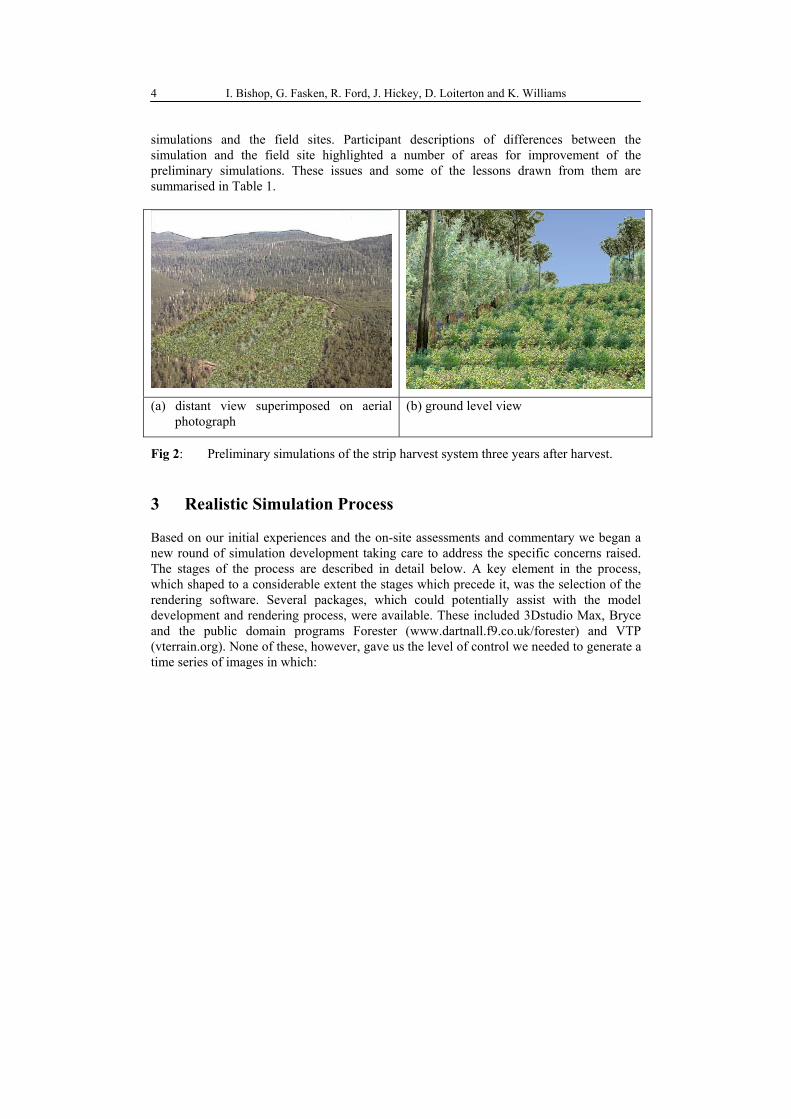
We anticipate play back at 2 frames per second to give a total run time of 1 minutes 40

seconds. However rate will also be tested before final evaluations are conducted. We

expect it will be appropriate to play each sequence twice before asking for responses.

Fig 5: Wide angle view of simulated forest at age 89 years.

3.5 Problems and Strategies

The single remaining difficulty with this production sequence is processing time. Both the

creation of the .pov files describing the forest condition and the rendering are taking

several hours on high end PC level equipment. We have several strategies under

development for speeding the processing. These include:

• progressive reduction in tree density at distances from the camera greater than 200

m for ground level views;

• omission of grasses and some other understory species in aerial views;

• reuse of mature forest frames when rates of growth and change are slow; and

• minimization of transparent areas within the texture files

4 Discussion

The field evaluation was critical to the process of developing simulations useful to the task

of assessing acceptability of forest management systems. The preliminary assessments were

exploratory, incorporating both quantitative and qualitative responses. They pointed to

specific aspects of the simulations that required further development in the context for

which they were developed. Comments on the simulations were made after participants had

judged the acceptability of the harvesting system at each field site, and explained their

reasons for these judgments. Comments on simulation accuracy were therefore closely

related to the criteria used in these judgments. The simulations were assessed by people

with diverse perspectives on the issue of forest management. This diversity was reflected in

their responses. For example, participants with an interest in the management of special

timber species (for example for boat building) were more likely to comment on the absence

of these species. The development of realistic simulations is constrained by resource

limitations including computing capacity. It is therefore vital that early, exploratory


evaluations be conducted to ensure the environmental characteristics that are included are

those most relevant to the purpose of the simulation. A diversity of views and knowledge

among the evaluators helps to ensure that the information content of the simulations meets

all needs.

5 Conclusion

Fierce public debate over forest management, as well as increased ecological knowledge,

has prompted forest agencies to develop and test alternative harvesting and regeneration

systems. This project is examining community response to these options through computer

simulation. It avoids the biases of existing research, based on a single temporal snap-shot

of projected forest condition, by allowing participants to view changes over time as the

forest regenerates.

Careful testing of preliminary simulations has proved to be extremely valuable in

establishing the key parameters of the simulation effort. However the very high density of

vegetation, of several different species, still provides a substantial challenge to our current

computer technology and landscape modelers.

6 References:

Bergen, R.D., Ulricht, C.A., Fridley, J.L. and Ganter, M.A. (1995). The validity of

computer-generated graphic images of forest landscape. Journal of Environmental

Psychology 15: 135-146.

Brown, M.J., Elliott, H.J. and Hickey, J.E. (2001). An overview of the Warra Long-Term

Ecological Research Site. Tasforests, 13: 1-8.

Florence, R.G. (1996). Ecology and silviculture of eucalypt forests. CSIRO, Collingwood,

Victoria.

Hickey, J.E., Neyland, M.G. and Bassett, O.D. (2001). Rationale and Design for the Warra

Silvicultural Systems Trial in wet Eucalyptus obliqua forests in Tasmania. Tasforests,

13: 155-182.

Karjalainen, E. and Tyrväinen, L. (2002) Visualization in forest landscape preference

research: a Finnish perspective, Landscape and Urban Planning, 59: 13-28

Muhar, A. (2001). Three-dimensional modelling and visualisation of vegetation for

landscape simulation. Landscape and Urban Planning 54: 5-18.

Myklestad, E. and J. A. Wager (1977). PREVIEW: computer assistance for visual

management of forested landscapes. Landscape Planning 4: 313-331.

Visualization of Vegetation Dynamics during the Holocene

Period for Educational Purposes

Reiner FUEST and Michael SCHNIRCH

1 Introduction

Changes in vegetation cover and land use, over time, are usually hard to imagine in detail, particularly for students. Two major problems exist: the difficulty of creating a mental image of the past situation and the long time periods over which processes are stretched.

Shorter time spans can sometimes be visualized by using “hard facts”, e.g. photographs, satellite imagery, cadastre datasets, ecological surveys. But dealing with thousands of years, only a “virtual” representation of the landscape can be created.

The aim of this study is to provide students with a visually appealing, yet (geo)scientifically sound representation of vegetation dynamics, so that the area “comes back to life” and that changes through time become apparent.

2 Motivation

This application has been developed for undergraduate students in geography courses. It therefore focuses mainly on educational effectiveness and the possible scenarios in which landscape and vegetation visualization provide significant benefits over more “classic” approaches. However, the word “students” could of course be replaced by “national park visitor”, “interested layman”, “someone who is new to a scientific concept” or, very often, “customer”.

Educational material will always be custom-made, because different audiences with specific needs have to be catered to and because the availability of information can hardly be generalized. Therefore, software and techniques used in research or production processes have to be adapted for this purpose. All too often, visualization used in courseware or lectureware is taken one-to-one from the visualized output of a lecturer’s research (KRYGIER ET AL.,1997; FRASER, 1999).

On the one hand, visualization technology is being pushed further and further in terms of technical perfection. On the other hand, concepts for making the results accessible in an appealing, and above all, educationally convincing way are scarce: “Data-driven

visualization and photo-realistic visualization are rapidly replacing tabular or verbal

information in public presentations and environmental impact statements. In each of these

cases however, information has most often been presented as images delivered to the user,

often with little description of the context in which they fit, and usually with no opportunity

to react and provide feedback” (ORLAND ET AL., 2001).

R. Fuest and M. Schnirch 2

Software currently available offers photo-realistic rendering, which is sufficient to give students a very good impression of “virtual” landscapes. But as TUFTE (1990) points out "High quality rendering does not necessarily aid understanding.” and GAHEGAN (1999) concludes “The use of abstraction may be more beneficial in terms of … increasing

cognition…".

Consequently, there is a great demand for the development of a user-interface that provides the learner with the most appropriate visual and multi-sensual stimuli for landscape interpretation. The development of such an access was identified by SLOCUM ET AL. (2001) as one of the major challenges for current visualization research.

In designing and developing a prototype for educational vegetation and landscape visualization, we make use of standard software tools to demonstrate their suitability for instructional design processes, but also to point out which elements have to be added in order to facilitate learning.

3 Conceptual Basis

Interactive multimedia learning resources contain many instances of educational visualization. But it is not enough merely to employ some visual elements indiscriminately. To facilitate the understanding of complex geoscientific concepts, the right choices have to be made concerning which methods of visualization are adequate in each case.

There have been several attempts to categorize geographic visualization elements. MACEACHREN (1994) introduces the idea of a “cartography cubed”, which provides a framework for distinguishing between private, highly interactive visual data exploration and public visual communication with limited interactivity. Dimensions of data representations are categorized by KRAAK & ORMELING (1996). KRYGIER ET AL. (1997) establish a matrix of resource functions and resource forms to classify educational resources. CRAMPTON (2002) puts the emphasis on interactivity types in geographic visualization.

Based on these categorizations, we identified three important problems to be solved:

The form of visual representation Current technology offers a wide range of possibilities: rather abstract diagrams or real imagery, 2D or 3D, animated or static – Which is appropriate? Which forms of data representation should be used? Does “more realistic” and “more sophisticated” equal “better”?

Interactivity Especially the question of navigation within a visual representation, but also issues of simulation have to be addressed: What kind and what degree of interactivity makes sense?

The combination of several representation forms Can one visual representation be sufficient? Which of the infinite possibilities of visualizing a model are to be presented to the learner? What can be done to help

Visualization of Vegetation Dynamics during the Holocene Period 3

the learner in building a better mental image of the spatio-temporal processes involved – and never lose his or her bearings in the process?

We will examine these questions with respect to vegetation modeling for educational purposes.

3.1 Using Different Representation Forms

The descriptions of vegetation dynamics throughout the Holocene Period are usually merely textual summaries of plant species and rough descriptions of their potential habitats at different points in time (Fig. 1). Even maps make it difficult to imagine how present landscapes looked in the past, just as it is almost impossible to recreate the look of an old street or historic building in one’s mind without the help of old photographs or films.

Here modern vegetation modeling tools can help tremendously: based on terrain and other geometric information, they are able to produce realistic-looking scenes of the past.

Among others LANGE (2001) and HIRTZ ET AL. (1999) showed that the inclusion of vegetation models greatly enhances the degree of realism, by which virtual landscapes are perceived by the user. As ZEH (2001) has demonstrated, this can also be transferred to (pre-) historic situations.

Fig. 1: Forest communities in the Southern Black Forest, Germany during the Holocene Period. Ab: Abies – fir; Ac: Acer – maple; Be: Betula – birch; Co: Corylus – hazel; Fa: Fagus – beech; Frax: Fraxinus – ash; Qu: Quercus – oak; Pi: Pinus – pine; Pic: Picea – spruce; Ti: Tilia – lime; Ul: Ulmus – elm (FRIEDMANN, 2000).

3.2 Interactivity Options

The term “interactivity” is overused and therefore carries many different meanings. For the scope of this paper we will use one of the simplest definitions, suggested by CRAMPTON


(2002): “…we will define interactivity … as a system that changes its visual data display in

response to user input.”

In this context, only a subset of interactivity options is considered: navigation, i.e. interaction with the data representation (as opposed to interaction with the data itself).

The question of navigation in different forms of cartographic representation in general has been subject of many publications (e.g. FUHRMANN & MACEACHREN, 1999; KRAAK, 2002). See CRAMPTON (2002) for an extensive review.

Providing the user with free navigation in all available display dimensions seems tempting, as it is feasible with current (web) technology (KRAAK, 2001; RIEDL, 2001; RIEDL ET AL., 2002). But objections to the option of free navigation in educational context have to be raised:

A change in perspective strongly influences a user's perception of a scene (GAHEGAN, 1999). A limited, quick to understand, yet sufficient set of navigation possibilities is more suited to point out important structures or objects. A set of optimal viewpoints can be chosen by the educator, and interactively selected by learners. Carefully chosen default settings might be more useful to communicate information (MACEACHREN, 1994; KRYGIER

ET AL., 1997).

Interaction with the temporal dimension, however, can be established with relative ease, as the concept of timelines controlled by slider bars is familiar to most computer users.

3.3 Multiple, Dynamically Linked Views

In computer gaming for example, virtual worlds have to be consistent only within themselves. In geographical education, the virtual representation has to be consistent with real world concepts. Moreover, landmarks for spatial and temporal orientation purposes have to be established. “Virtual” viewpoints (birds-eye, overhead etc.) have to be linked to viewpoints known from the learner’s everyday life.

To provide insight into the interrelations between different data representations the linking of views is of major importance. VERBREE ET AL. (1999) and KRAAK (2002) applied this idea to virtual reality worlds. DYKES (2002) describes a simpler method using geo-referenced digital panoramic imagery. According to them, 2D maps (“map view”), bird’s-eye 2,5D perspective views (“plan views”) and 3D-Virtual Reality elements (“world

views”) should be combined. In addition to this, changes made in one data representation are instantly displayed in the other displays. This enables users to develop a better idea of space in virtual reality environments.

4 Vegetation Modeling

4.1 Study Area: The Zastler Valley, Black Forest

The Zastler Valley is located on the northern slope of the Feldberg (1493 m asl), the highest peak in the Black Forest, Southern Germany.


Glaciation during the last ice-age in the Southern Black Forest was restricted to the shallow ice cap of the Feldberg and the surrounding mountain peaks with their outlet glaciers in the valleys. During the maximum extent of the last glaciation, the glacier in the Zastler Valley reached about 5 km in length and several hundred metres in height. The snow line lay around 900 m asl. Cirque glaciers on the north facing slopes still existed during the early Holocene Period (METZ, 1997).

Fluvial geomorphologic processes dominated during the Holocene Period. The low lying erosion base, i.e. the Rhine river, in combination with high precipitation levels caused high rates of fluvial erosion in the area. The intensity varied with the amount of available water and density of vegetation cover (MÄCKEL, 1997).

The immigration of plants and especially trees during the late Pleistocene and early Holocene Periods is strongly correlated with climate parameters. Predominant vegetation types are shown in Fig. 1. For a thorough discussion see FRIEDMANN (2000).

During the last 1200 years, human impact, especially herding, logging and charburning has fundamentally altered the ecological parameters. A fact which is reflected in the composition of vegetation communities and the extent of vegetation cover (WILMANNS, 2001; LUDEMANN, 2001).

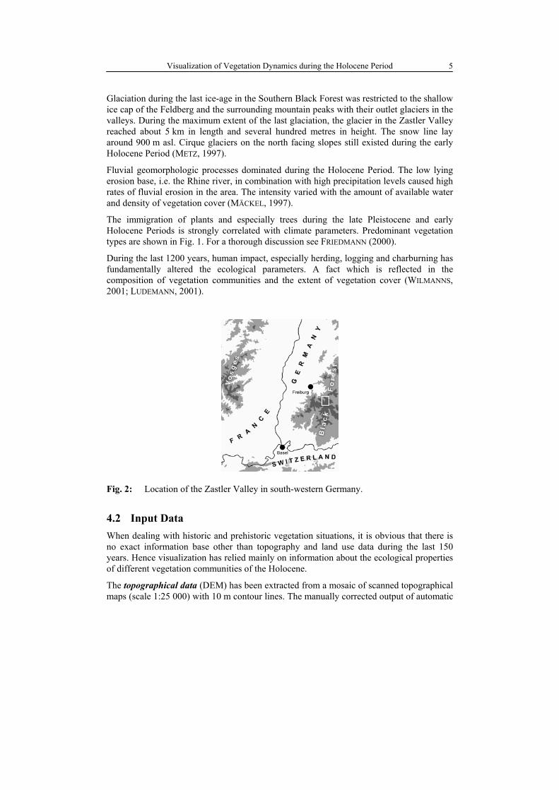
Fig. 2: Location of the Zastler Valley in south-western Germany.

4.2 Input Data

When dealing with historic and prehistoric vegetation situations, it is obvious that there is no exact information base other than topography and land use data during the last 150 years. Hence visualization has relied mainly on information about the ecological properties of different vegetation communities of the Holocene.

The topographical data (DEM) has been extracted from a mosaic of scanned topographical maps (scale 1:25 000) with 10 m contour lines. The manually corrected output of automatic


vectorization has been triangulated to form a Triangular Irregular Network (TIN), from which a 5 m resolution raster data set has been derived (for details see ZHU ET AL., 1999; EASTMAN, 1999).

Historic climatological data on the distribution, extent and retreat of glaciers, average temperature and rainfall etc. have been derived from the works of BOGENRIEDER (1982), METZ (1997), LIEHL (1989) and SCHÖNWIESE (1995).

Historic ecological data, e.g. information on species, vegetation communities and their distribution during several stages of the Holocene, have been derived from FRIEDMANN

(1997 and 2000) and LUDEMANN (2001).

3D-Plant-Models and photo-realistic representations of plant species have been taken from the “Exteriors” add-on CD for Maxon Cinema 4D® and the World Construction Set® 6 foliage collection.

Photographs have been taken by the authors during field trips.

4.3 Vegetation and Landscape Modeling

We use a GIS-based approach as suggested by MUHAR (2001) and LANGE (2001), because of the high importance of mid- and far-range visualization output based on terrain factors such as height asl, aspect and slope. Therefore, no information about the exact location of vegetation communities or even individual plants is needed. They can be modelled by specifying the ecologically relevant factors for vegetation growth. This is very important, as existing information about vegetation communities during the late Pleistocene and most of the Holocene is restricted to lists of species related to certain terrain elevations, which were almost entirely derived from pollen and charcoal analysis (FRIEDMANN, 1997).

The human impact, although clearly proven (WILMANNS, 2001; LUDEMANN, 2001), has been modelled in a way such as to visualize the overall man-made changes in vegetation cover density and species distribution rather than the exact details of the historic situation.

5 Results

5.1 Educational Landscape Visualization

Experiments with vegetation and landscape visualization for educational purposes in undergraduate teaching have lead to the following results which have been implemented in a prototype version of a multimedia application presented below.

First, we suggest the integration of data representations with different levels of abstraction and dimensionality (photo, photo-realistic-rendering, perspective map-like rendering and conventional maps or satellite images; 2D to 4D). Each one on its own is less powerful than in combination. A high degree of realism is important to make the final product visually appealing and interesting. Modern tools for vegetation and landscape modeling are very useful in creating photo-realistic images from virtual worlds. On the other hand, the level of abstraction of the landscape representation has to be chosen very carefully so that the learners are not distracted from the scientific concept the understanding of which


should be promoted. Another point is, that it is very time consuming to produce good-looking and scientifically sound landscape models.

Second, we encourage developers not to fall for the technically feasible, but in use limited set of interactive navigation options. Learners will probably get more confused than they benefit from the freedom to adjust perspectives to their liking. Attention is easily distracted from the important facts or concepts.

Third, by linking multiple views, one can create more than merely a combination of different representation forms. General orientation and the discrimination of specific objects or landscape features will be trained by placing particular emphasis on transfer of representations from 2D to 3D (SIEBER, 2001). This concept can help students to develop a "visual literacy" in geography to "understand visual grammar (which) is important

because it enables us to understand and imagine" (AITKEN,1999).

5.2 Multimedia Learning-Object

The actual production of the visualization output relies on standard 3D landscape modeling tools. The software package World Construction Set® 6 provides appropriate vegetation and landscape modeling functionality for our needs. The interactive linking of the representation components is realized in the multi-media authoring environment Macromedia Flash MX® and web-enabled using the open Shockwave Flash® (*.swf) file format. A working prototype of the application can be accessed at http://www.webgeo.de/papers/2003/dessau/ .

Fig. 3: A screenshot of the application prototype, interactively linking the different landscape model representations (see http://www.webgeo.de/papers/2003/dessau/ for an online version).


In pursuit of the initial approach, most of the ideas postulated in section three have been implemented.

Photo-realistic landscape visualization output in the form of virtual panoramas is combined with map-like perspective views, 2D overview maps and timeline diagrams. Three views are displayed at a time. These different forms of data representations are dynamically linked to display changes in real-time.

The learner can interact with the temporal dimension of the data display by dragging the slider on the time scale. Spatial navigation tools are available through toggling functions on the map, through the selection of different viewpoints for the birds-eye view, and through 360° panorama videos. As a result, different aspects of the landscape as a whole can be perceived simultaneously.

6 Conclusions & Outlook

The conceptual framework presented here is an attempt to facilitate the understanding of vegetation dynamics in educational contexts by combining different dynamically linked data representations. These data representations differ in their level of abstraction, dimensionality of representation and degree of interactivity.

It is shown that to fully access the potential of photo-realistic output of modern landscape visualization tools, such imagery should always be associated with more abstract forms of data representations (e.g. maps and graphs). This will significantly enhance the ability of learners to develop an understanding of the depicted space and change over time.

Formative evaluation is currently being carried out, based mainly on the results of student questionnaire feedback. Most comments so far are very encouraging. A final evaluation is scheduled for end of summer-term 2003.

The application will be embedded in an online geography course module and not be accessible as a stand-alone version.

Further refinements of the data display and the degree of interactivity could lead in two directions: The provision of possibilities to delve deeper into the topic of vegetation development and climate change, e.g. by providing and linking other related learning resources, and the use of audio support to enhance immersion (e.g. by exemplifying cold temperature through chilling wind) as well as information access (spoken commentary).

7 Acknowledgements

This research was part of the project “WEBGEO – Webbing of Geoprocesses for Undergraduate Earth-Science Education”, funded by the German Federal Ministry of Education and Research (BMBF).


Inquiries regarding historic vegetation development were kindly answered by R. Glawion, Institut für Physische Geographie University of Freiburg and A. Friedmann, Institut für Geographie University of Augsburg.

We would also like to thank the teams of WEBGEO|vegetation and WEBGEO|klima, especially A. Kalt for his helpful and inspiring comments. A. Mack helped substantially code the multimedia framework.

8 References

Aitken, S. C. (1999): Scaling the light fantastic: geographies of scale on the web. Journal of Geography, 98: 118-127.

Bogenrieder, A. (1982): Der Feldberg im Schwarzwald : subalpine Insel im Mittelgebirge. LfU, Karlsruhe.

Crampton, J. W. (2002): Interactivity types in geographic visualization. Cartography and Geographic Information Science, 29(2): 85 - 98.

Dykes, J. (2002): Creating information-rich virtual environments with geo-referenced

digital panoramic imagery. In: P. Fisher & D. Unwin (eds.): Virtual reality in geography. Francis & Taylor, London.

Eastman, J. R. (1999): Guide to GIS and image processing. Clark Labs, Worcester. Fraser, A. B. (1999): Colleges should tap the pedagogical potential of the world-wide web.

The chronicle of higher education, 48(8): B8. Friedmann, A. (1997): Spät- und postglaziale Waldgeschichte des südlichen

Oberrheintieflands und Schwarzwalds. In: R. Mäckel & B. Metz (eds.): Schwarzwald und Oberrheintiefland. Eine Einführung in das Exkursionsgebiet um Freiburg im Breisgau. Geographische Institute der Albert-Ludwigs-Universität Freiburg im Breisgau

Friedmann, A. (2000): Die spät- und postglaziale Landschafts- und Vegetationsgeschichte

des südlichen Oberrheintieflands und Schwarzwalds. Institut für Physische Geographie, Albert-Ludwigs-Universität Freiburg i. Br., Freiburg i. Br.

Fuhrmann, S. & A. M. MacEachren (1999): Navigating Desktop GeoVirtual Environments. IEEE Information Visualization '99. San Francisco.

Gahegan, M. (1999): Four barriers to the development of effective exploratory

visualization tools for the geosciences. International Journal of Geographical Information Science, 13(4): 289-309.

Hirtz, P., H. Hoffmann & D. Nüesch (1999): Interactive 3D landscape visualization:

improved realism through use of remote sensing data and geoinformation. Computer Graphics International, Canmore, Canada. .

Kraak, M. J. & F. Ormeling (1996): Cartography: visualization of spatial data. Longman, Singapur.

Kraak, M. J. (2001): 3-D-mapping on the World Wide Web. In: R. Buzin & Wintges, T. (eds.): Kartographie 2001 - multidisziplinär und multimedial. Wichmann, Heidelberg.

Kraak, M. (2002): Visual exploration of virtual environments. In: P. Fisher & Unwin, D. (eds.): Virtual Reality in Geography. Taylor & Francis, London.


Krygier, J. B., C. Reeves, D. DiBiase & J. Cupp (1997): Design, implementation and

evaluation of multimedia resources for geography and earth science education. Journal of Geography in Higher Education, 21(1): 53-71.

Lange, E. (2001): The limits of realism: perceptions of virtual landscapes. Landscape and urban planning, 54: 163-182.

Liehl, E. (1989): Der Schwarzwald. Beiträge zur Landeskunde. Konkordia Verlag, Bühl/ Baden.

Ludemann, T. (2001): Das Waldbild des Hohen Schwarzwaldes im Mittelalter: Ergebnisse

neuer holzkohleanalytischer und vegetationskundlicher Untersuchungen. Alemannisches Jahrbuch, 1999/00: 43-64.

MacEachren, A. M. (1994): Visualization in modern cartography. Pergamon, Oxford. Metz, B. (1997): Glaziale Formen und Formungsprozesse im Schwarzwald. In: R. Mäckel

& B. Metz (eds.): Schwarzwald und Oberrheintiefland. Eine Einführung in das Exkursionsgebiet um Freiburg im Breisgau. Geographische Institute der Albert-Ludwigs-Universität Freiburg im Breisgau, Freiburg i. Br.

Muhar, A. (2001): Three-dimensional modeling and visualization of vegetation for

landscape simulation. Landscape and Urban Planning, 54: 5-17. Mäckel, R. (1997): Spät- und postglaziale Flußaktivität und Talentwicklung im

Schwarzwald und Oberrheintiefland. In: R. Mäckel & B. Metz (eds.): Schwarzwald und Oberrheintiefland. Eine Einführung in das Exkursionsgebiet um Freiburg im Breisgau. Geographische Institute der Albert-Ludwigs-Universität Freiburg im Breisgau

Orland, B., K. Budthimedhee & J. Uusitalo (2001): Considering virtual worlds as

representations of landscape realities and as tools for landscape planning. Landscape and urban planning, 54: 139-148.

Riedl, A. (2001): Virtual Reality - die zukünftige Realität der Geokommunikation? In: R. Buzin & T. Wintges (eds.): Kartographie 2001 - multidisziplinär und multimedial. Wichmann, Heidelberg.

Riedl, A., G. Katzlberger & H. Tomberger (2002): Entwicklungs-/Modellierumgebungen

für Web-basierte Geo-Virtual Reality Applikationen - eine Gegenüberstellung.

CORP2002 & GeoMultimedia02: Who plans Europe´s future? Wien. Schönwiese, C. (1995): Klimaänderungen : Daten, Analysen, Prognosen. Springer,

Heidelberg. Sieber, R. (2001): Interdisziplinarität und Multidimensionalität in thematischen Atlanten.

In: R. Buzin & T. Wintges (eds.): Kartographie 2001 - multidisziplinär und multimedial. Wichmann, Heidelberg.

Slocum, T. A., C. Blok, B. Jiang, A. Koussoulakou, D. R. Montello, S. Fuhrmann & N. R. Hedley (2001): Cognitive and usability issues in geovisualization. Cartography and Geographic Information Science, 28(1): 61-75.

Tufte, E. R. (1990): Envisioning information. Graphics Press, Cheshire. Verbree, E., G. Van Maren, R. Germs, F. Jansen & M. J. Kraak (1999): Interaction in

virtual world views - linking 3D GIS with VR. International Journal of Geographical Information Science, 13(4): 385-396.

Wilmanns, O. (2001): Exkursionsführer Schwarzwald - eine Einführung in Landschaft und

Vegetation. Ulmer, Stuttgart. Zeh, M. (2001): Photorealistische 3D-Visualisierung am Beispiel der spät- und

postglazialen Landschafts- und Vegetationsentwicklung im Südschwarzwald. Geographisches Institut der Ruprecht-Karls-Universität Heidelberg, Heidelberg.


Zhu, H., J. R. Eastman & K. Schneider (1999): Constrained delaunay triangulation and

TIN optimization using contour data. Proceedings of the thirteenth international Conference on applied geologic remote sensing. Vancouver, Canada.

"Non-Geometric" Plant Modeling: Image-Based Landscape

Modeling and General Texture Problems with Maya -

Examples and Limitations

Peter OEHMICHEN

1 Introduction

When starting a new visualization project, one has to think about the demands of the

project and the possibilities and resources one already has at hand. Before starting to

develop something completely new, it is quite often useful to consider the available

computer program features that are not often used, specifically plug-ins or combinations of

programs. Instructions and tips from other program sources are often adaptable without too

much effort and are relatively simple and effective to use. And while not everyone is an

experienced programmer, it can be a good idea to call in outside help. This can lengthen the

whole process, but there are many dealing with the same kind of problems and sometimes

they have the time (and get paid) to develop the perfect or almost perfect solution. One of

the programs with features that are helpful for a large landscape visualization is Maya with

Paint Effects.

What does Paint Effects of Maya have that could be of interest, one might well ask. The

author believes it offers a solution to fill the gap that sometimes arises between geometric

and “non-geometric” plant representations. And it is a built-in feature of a standard

package for visualization purposes. To create different kinds of visualization without using

a very specific landscape visualization software product, one can use one of the largely

available tools such as Max, Cinema4D, LightWave or even Maya. Like the other tools,

Maya is usable for all kinds of standard visualization and animation tasks and like all the

others it has specific advantages and weaknesses or limitations. The author, as well as other

users, always concentrates on the advantages and specific features of the software already

being used because that is the reason it was selected.

2 Vegetation Modeling

The main topic of this article is vegetation modeling. The “non-geometric” in the title does

not mean there is no geometric information, but that the focus is on additional data and

information needed to create or show a visual representation of a plant. This could be

texture information (image representation) or a procedural instruction to automatically

create a plant species. Highly differentiated and therefore difficult to compute objects with

a large number of triangles/faces should be avoided.

P. Oehmichen 2

2.1 Scale Dependencies

The kind of visual representation to be chosen depends on the distance to the object to be

represented. The triangle, as the simplest geometric form, is suitable to present a texture.

With more complicated texture/shape outlines, it is possible to choose a quadrate. Normally

it is best suited for large numbers of plant objects in the distance. As you come closer to the

object, more details can be seen and have to be added. Conventionally it is done by a

greater geometric differentiation and smaller pieces of texture (despite the option to

enhance the texture resolution). The number of faces necessary to represent the plant/tree

rises from the minimum of 1 to tens of thousands with a great influence on render times

while the textures differ only slightly in size. Paint Effects plants are positioned only in

space with the help of curves and do not contain any geometric faces. They can have a

different degree of refinement and therefore require more or less rendering time but less

than “true” 3D-models

2.2 Maya Paint Effects

2.2.1 What is Behind Paint Effects

Paint Effects is procedural determined (a kind of L-system). It is a particle trace with

defined splitting points. The particle is then replaced by a so called splat (airbrush stamps)

with different color settings and written into a special memory buffer. Finally, everything is

rendered as a post process after standard scanline rendering. This results in low memory

consumption and fast rendering speeds. It offers many of possibilities to achieve a variety

of different visual effects, not only in vegetation models, but also in things such as clouds,

fire and smoke, liquids and so on.

2.2.2 The Procedural Structure

In Maya’s node-based structure one has 3 nodes for the particular Paint Effect result: a

general transform node, a stroke shape node and a brush node. There is also a curve node

for the positioning of the Paint Effect in World Space coordinates. The most interesting

node for the effect itself (and the plant of course) is the brush node. Important attribute

settings will be highlighted as examples.

Fig. 1: Hypergraph window with node relationship

"Non-Geometric" Plant Modeling: Image-based Landscape Modeling 3

Fig. 2: Transform node (stroke example): Contains the basic information about

positioning, rotating and scaling.

The general node for the positioning etc. in relation to the World Coordinate System or

hierarchical higher levels is the Transform node. More important than the Transform node

is the Shape node. It contains information about the Display Quality in the standard view

ports, Sample Density (how many pieces per unit), Seed (shape variations under the same

stroke settings), Surface Offset, End Bounds (used parts of the curve), Normal Direction,

Pressure Mapping (variations in size, elevation etc. by a pressure curve derived from stylus

pressure or edited curve points) and more.

Fig. 3: Shape node (strokeShapeExample)

The most important node for the creation of the desired plant species, as mentioned above,

is the brush node. It contains about 250 settings for the final look of the plant or effect, but

it is not necessary to use all of them. Brush Type is for Paint (Effects), and Global Scale is

P. Oehmichen 4

for proportional adjustments of height and width. The main sections are: Brush Profile for

the width of the effects including some twisting and stamp density (the splats), Shading for

the color and texture settings, Illumination for the light setting (real or faked single

direction) and some translucence and specular shading, Shadow Effects (faked 2D or 3D),

Glow for light effects, Tubes for the procedural growth of the object (explained more in

depth later), Gaps for any open spaces in the sequence of splats and Flow Animation for

some animated growth like effects.

Fig. 4: Brush node (overview)

Tubes gives the possibility to extend the stroke into the 3rd dimension. With Tube

Completion activated, the plant at the end of the stroke grows to its full extent. The

Creation section gives all necessary information for the first tube (or the trunk) and with

the Growth section it can be divided into finer structures. The Behavior section gives the

opportunity to add some irregular movement over time and reaction to applied forces.

Fig. 5: Tubes section

In the Creation section one can set the density, initial number, size (length and width),

number of segments, direction, elevation and azimuth of the tubes. Together with the

Shading and Texturing section, it forms the base for the Branch and Twigs creation in the

Growth section.


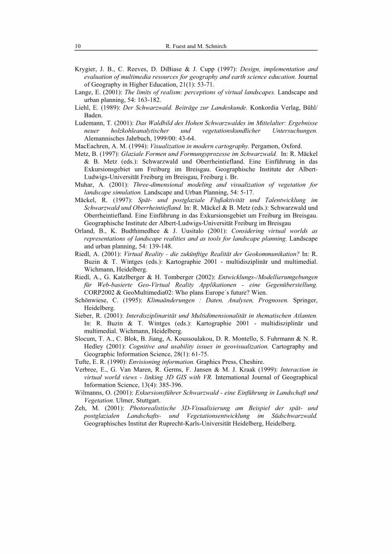
Fig. 6: Creation section

In the Growth section one can decide to have all or part of the possible elements: Branches,

Twigs, Leaves, Flowers and Buds, with each again having its own collection of attributes

to adjust in order to achieve the desired look.

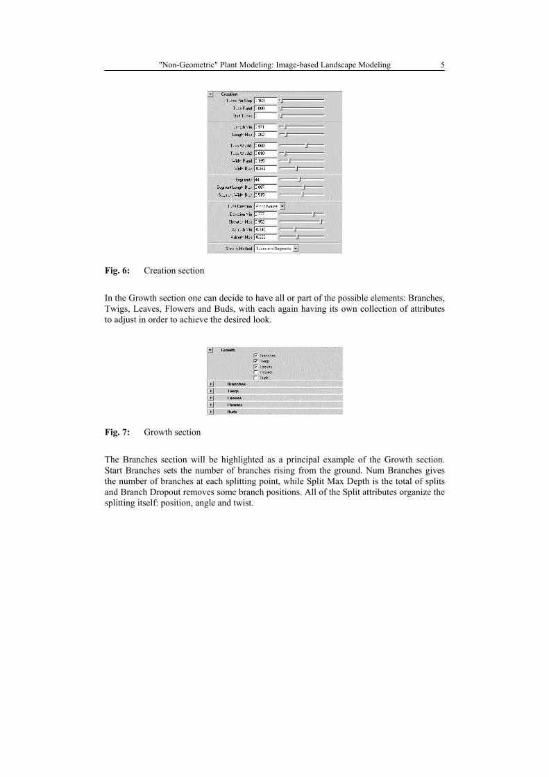
Fig. 7: Growth section

The Branches section will be highlighted as a principal example of the Growth section.

Start Branches sets the number of branches rising from the ground. Num Branches gives

the number of branches at each splitting point, while Split Max Depth is the total of splits

and Branch Dropout removes some branch positions. All of the Split attributes organize the

splitting itself: position, angle and twist.

P. Oehmichen 6

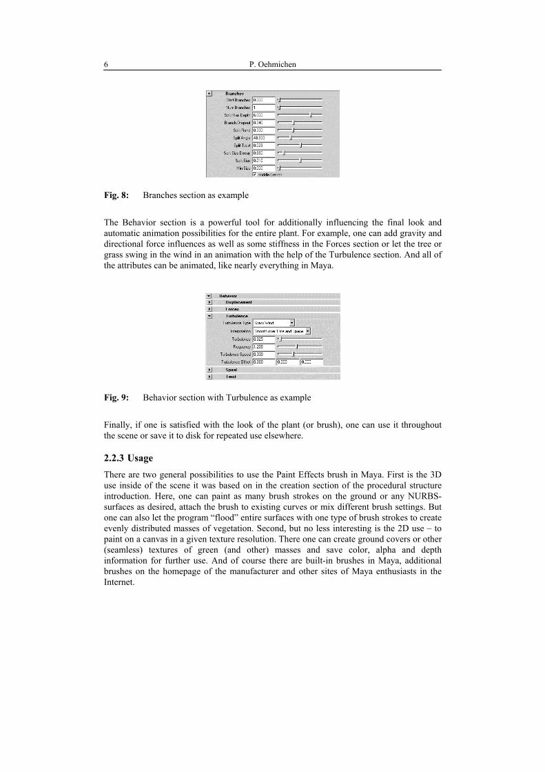
Fig. 8: Branches section as example

The Behavior section is a powerful tool for additionally influencing the final look and

automatic animation possibilities for the entire plant. For example, one can add gravity and

directional force influences as well as some stiffness in the Forces section or let the tree or

grass swing in the wind in an animation with the help of the Turbulence section. And all of

the attributes can be animated, like nearly everything in Maya.

Fig. 9: Behavior section with Turbulence as example

Finally, if one is satisfied with the look of the plant (or brush), one can use it throughout

the scene or save it to disk for repeated use elsewhere.

2.2.3 Usage

There are two general possibilities to use the Paint Effects brush in Maya. First is the 3D

use inside of the scene it was based on in the creation section of the procedural structure

introduction. Here, one can paint as many brush strokes on the ground or any NURBS-

surfaces as desired, attach the brush to existing curves or mix different brush settings. But

one can also let the program “flood” entire surfaces with one type of brush strokes to create

evenly distributed masses of vegetation. Second, but no less interesting is the 2D use – to

paint on a canvas in a given texture resolution. There one can create ground covers or other

(seamless) textures of green (and other) masses and save color, alpha and depth

information for further use. And of course there are built-in brushes in Maya, additional

brushes on the homepage of the manufacturer and other sites of Maya enthusiasts in the

Internet.


2.2.4 Limitations

The main limitation is the “lack of precision” in the distribution of the splats which is the

cause for a loss of realism in very close-up shots. Furthermore, it is impossible to

classically animate individual parts of the plant. And due to the specific internal structure

of Paint Effects, there are some other limitations as well. It can also not be used with ray

tracing as it is a post effect. Therefore it is not possible to have any reflections, refractions

or ray traced shadows directly. You need to use depth map shadows, reflection maps and

sometimes a number of render passes to achieve these effects.

Even if the technology behind Paint Effects is optimized for speed and memory usage,

things can slow down if one has large numbers of tiny elements that are rarely seen. Partial

or general texture use (for tubes or leaves) can help to solve that problem.

As with all other renderings, artifacts and unwanted effects can appear and one has to look

for workarounds. But again, one can get help from the online help or documentation, the

hotline, in user groups or on web pages …

2.2.5 Examples

A few examples should give a better impression on the general ways of using Paint Effects

plants. First is the ground cover painted in 2D and then applied as texture to a plane. In the

foreground, a 3D grass can be added to improve the look. For further refinement even more

different plants can be added.

Fig. 10: Color, Alpha and Depth (Bump) file

Fig. 11: Perspective view of ground cover and with additional 3D grass

P. Oehmichen 8

Fig. 12: Medium size flower added, Delphinium type and with Dandelion fruit stand

The next example is a Birch tree from the built-in collection of brushes. It uses texture

information for the bark but not for the leaves. As a 3D brush it is set on the surface of the

underlying landscape. Rendered alone against the background it can be used for the Paint

Effects or billboard texture. If one would like to have it animated like the original Paint

Effects tree it is no problem to use an image sequence or movie file. The use for level of

detail solutions (LODs) is not recommended because of popping effects due to the greater

variations of the Paint Effects trees.

Fig. 13: Birch tree as Paint Effects and as texture (no shadow)

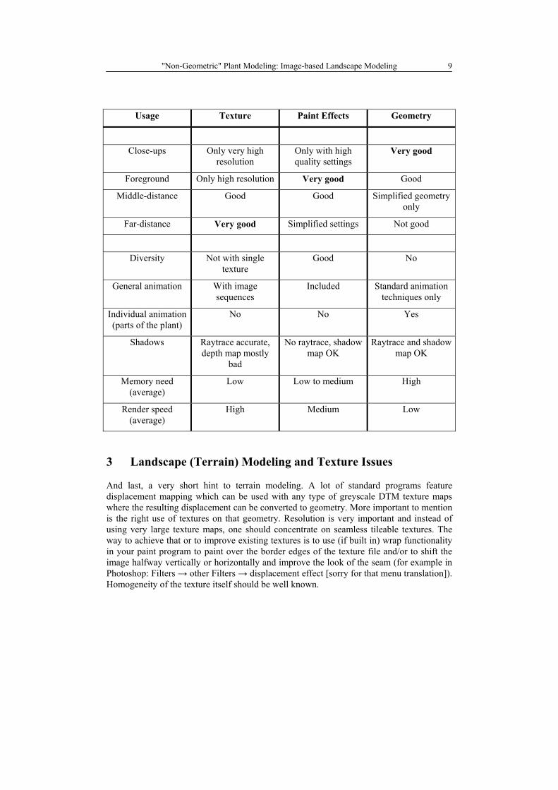
2.3 Texture vs. Geometry vs. Paint Effects

There is no single solution for every problem, but this overview provides some

recommendations and is therefore to be viewed as a reference for each individual decision.

As mentioned earlier, there are always possibilities to combine techniques to achieve the

optimal solution for a specific problem. Even with one technique it is possible to use

different quality settings. A rule of thumb is to start with textures (billboard or Paint

Effects) and if it does not look good enough, then continue with Paint Effects rather than

geometry. Only for individual animations of parts of a plant are geometric plants necessary.


Usage Texture Paint Effects Geometry

Close-ups Only very high

resolution

Only with high

quality settings

Very good

Foreground Only high resolution Very good Good

Middle-distance Good Good Simplified geometry

only

Far-distance Very good Simplified settings Not good

Diversity Not with single

texture

Good No

General animation With image

sequences

Included Standard animation

techniques only

Individual animation

(parts of the plant)

No No Yes

Shadows Raytrace accurate,

depth map mostly

bad

No raytrace, shadow

map OK

Raytrace and shadow

map OK

Memory need

(average)

Low Low to medium High

Render speed

(average)

High Medium Low

3 Landscape (Terrain) Modeling and Texture Issues

And last, a very short hint to terrain modeling. A lot of standard programs feature

displacement mapping which can be used with any type of greyscale DTM texture maps

where the resulting displacement can be converted to geometry. More important to mention

is the right use of textures on that geometry. Resolution is very important and instead of

using very large texture maps, one should concentrate on seamless tileable textures. The

way to achieve that or to improve existing textures is to use (if built in) wrap functionality

in your paint program to paint over the border edges of the texture file and/or to shift the

image halfway vertically or horizontally and improve the look of the seam (for example in

Photoshop: Filters s other Filters s displacement effect [sorry for that menu translation]).

Homogeneity of the texture itself should be well known.

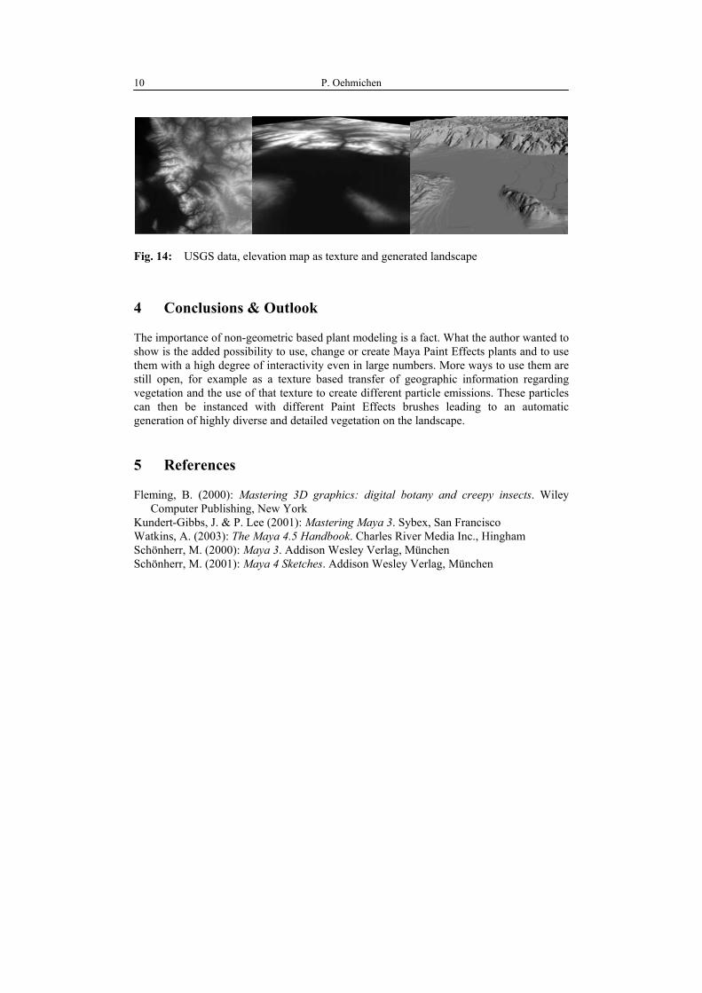
P. Oehmichen 10

Fig. 14: USGS data, elevation map as texture and generated landscape

4 Conclusions & Outlook

The importance of non-geometric based plant modeling is a fact. What the author wanted to

show is the added possibility to use, change or create Maya Paint Effects plants and to use

them with a high degree of interactivity even in large numbers. More ways to use them are

still open, for example as a texture based transfer of geographic information regarding

vegetation and the use of that texture to create different particle emissions. These particles

can then be instanced with different Paint Effects brushes leading to an automatic

generation of highly diverse and detailed vegetation on the landscape.

5 References

Fleming, B. (2000): Mastering 3D graphics: digital botany and creepy insects. Wiley

Computer Publishing, New York

Kundert-Gibbs, J. & P. Lee (2001): Mastering Maya 3. Sybex, San Francisco

Watkins, A. (2003): The Maya 4.5 Handbook. Charles River Media Inc., Hingham

Schönherr, M. (2000): Maya 3. Addison Wesley Verlag, München

Schönherr, M. (2001): Maya 4 Sketches. Addison Wesley Verlag, München

visual simulation of forest regrowth under different ... · pdf filevisual simulation of...

Documents