visualization and analysis of eddies in a global ocean...

Eurographics / IEEE Symposium on Visualization 2011 (EuroVis 2011)H. Hauser, H. Pfister, and J. J. van Wijk(Guest Editors)

Volume 30(2011), Number 3

Visualization and Analysis of Eddies in a Global OceanSimulation

S. Williams1,2, M. Hecht1, M. Petersen1, R. Strelitz1, M. Maltrud3, J. Ahrens1, M. Hlawitschka2, and B. Hamann2

1Computer, Computational and Statistical Sciences Division,Los Alamos National Laboratory2Institute for Data Analysis and Visualization (IDAV), Department of Computer Science, University of California, Davis

3Theoretical Division, Los Alamos National Laboratory

AbstractWe present analysis and visualization of flow data from a high-resolution simulation of the dynamical behavior ofthe global ocean. Of particular scientific interest are coherent vorticalfeatures called mesoscale eddies. We firstextract high-vorticity features using a metric from the oceanography community called the Okubo-Weiss parame-ter. We then use a new circularity criterion to differentiate eddies from other non-eddy features like meanders instrong background currents. From these data, we generate visualizations showing the three-dimensional structureand distribution of ocean eddies. Additionally, the characteristics of each eddy are recorded to form an eddy cen-sus that can be used to investigate correlations among variables such as eddy thickness, depth, and location. Fromthese analyses, we gain insight into the role eddies play in large-scale ocean circulation.

Categories and Subject Descriptors(according to ACM CCS): Computer Graphics [I.3.8]: Applications—Oceanography Simulation and Modeling [I.6.6]: Simulation Output Analysis—Ocean General Circulation Models

1. Introduction

Oceanography in the early and mid-20th Century was fo-cused on the description and analysis of the mean circula-tion. This changed later in the century as new observationsproduced evidence of a surprisingly vigorous field of of-ten long-lived and deeply penetrating vortices, referred toas mesoscale eddies. Satellite-based sea surface height al-timetry soon produced nearly global maps on which the sur-face signature of these vortices was clearly evident. Spectralanalysis indicated that a large fraction of the total estimateof oceanic kinetic energy is associated with these mesoscaleeddies [FS96], transforming our understanding of the fluiddynamics of ocean circulation.

Oceanic eddies are typically understood as vortices thatare 50-200 km in diameter, may live for several months, andcan propogate across an ocean basin. They are most numer-ous near strong currents like the Gulf Stream, Kuroshio Cur-rent, and Antarctic Circumpolar Current. These eddies havea significant influence on the earth’s climate: they transportheat, freshwater, momentum, and mass [LBM02, VLF08].The flow around eddies isolates the interior waters from thesurrounding ocean; shipboard studies have measured higherconcentrations of carbon, oxygen, and biologically impor-

tant nutrients within eddies [MPH∗07]. These nutrients areoften transported by the eddies to nutrient-poor waters, in-creasing the productivity of the food chain.

Around the time that satellite-borne altimeters began pro-ducing near-global observations of sea surface height, oceangeneral circulation models (OGCMs) crossed into a higherresolution regime in which the mesoscale eddies began to beresolved. These models are closely related to those used innumerical weather prediction and atmospheric modeling ingeneral, and the ancestry of the first OGCM [Bry69] oweda great deal to earlier work on numerical modeling of geo-physical fluid dynamics for atmospheric science.

The first realistic eddying ocean model simulations fo-cused regionally on the Southern Ocean [FRA91] and on theNorth Atlantic [BH89]. A spectral analysis of an approxi-mately 1

4◦

resolution model, based on the average horizon-tal spacing between grid points, showed a model sea sur-face height variability that was lower than that derived fromthe altimeter by approximately a factor of two [FS96]. Ascomputing power increased, first regional and then globalmodels could be configured and run at horizontal grid reso-lutions of around 1

10◦

, and their mesoscale variability wasfound to come into much better agreement with observa-

c© 2011 The Author(s)Journal compilationc© 2011 The Eurographics Association and Blackwell PublishingLtd.Published by Blackwell Publishing, 9600 Garsington Road, Oxford OX4 2DQ, UK and350 Main Street, Malden, MA 02148, USA.

S. Williams, M. Hecht, M. Petersen, et al / Global Eddy Analysis and Visualization

(a) (b)

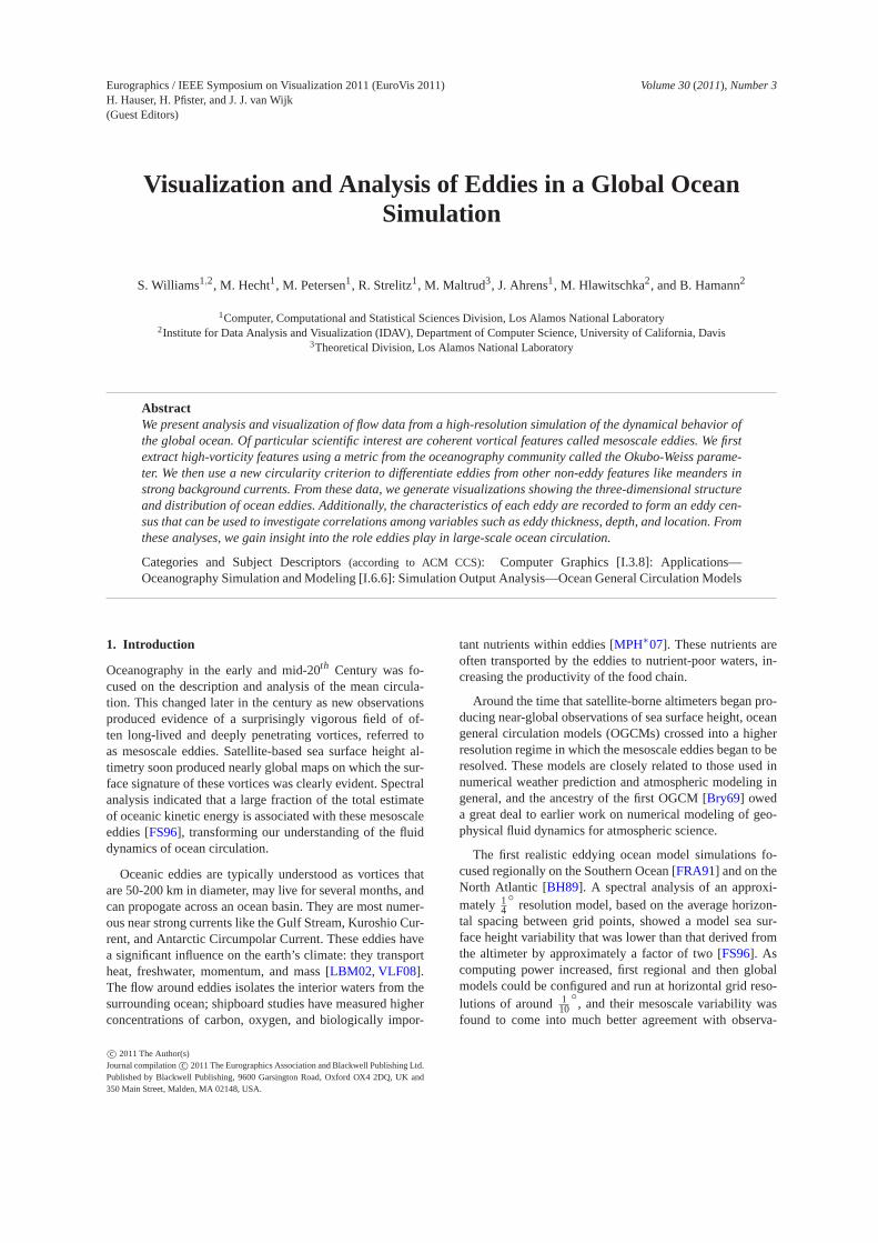
Figure 1: (a) The Okubo-Weiss parameter, a standard metric in oceanography for extracting two-dimenisonal vortices, at theocean surface in the North Atlantic. In order to keep scaling consistent, the Okubo-Weiss value is normalized to its standarddeviation. Red regions are those dominated by vorticity, while blue regions are those dominated by strain. The Okubo-Weissparameter easily identifies several eddies as red circles, but non-eddy meanders in the Gulf Stream are detected as well.(b) TheOkubo-Weiss parameter visualized at depth by removing all low-vorticity points. The three-dimensional shapes of the eddiesare now made clear: in the region containing the Gulf Stream, several strong eddies reach very deeply into the ocean, whilesmaller eddies remain near the surface, and the Gulf Stream itself only dominates near the surface.

tions [SMBH00,MM05]. The mean currents also came intomuch better agreement with observations in terms of width,speed and depth. The Gulf Stream, running from the FloridaStraits and departing from the continental shelf at Cape Hat-teras, then feeding into the northward-turning North AtlanticCurrent, showed great improvement in path, an indication ofthe essential role of eddy-mean flow feedbacks in determin-ing the large scale circulation.

Computer modeling of ocean circulation and modern ob-serving programs together have produced major advancesin physical oceanography. Ocean models save full three-dimensional data fields, but publications in oceanographytypically show simple two-dimensional plots of variables onthe surface and in vertical sections. This is partly becauseoceanographers are familiar with these views from observa-tional studies, and partly due to the limitations of the visu-alization tools that oceanographers typically use. Horizontalvelocities in the ocean are 1000 times larger than vertical ve-locities, so 2D horizontal sections are often the best way todisplay the ocean’s currents. A notable exception is the verti-cal structure of eddies. Questions about their vertical extent,tilt, and tapering require three-dimensional analysis and vi-sualization.

To this end, we performed parallel analysis on high-resolution ocean simulation data on a local computing clus-

ter, extracting eddies and visualizing them in the vicinityof one of the world’s strongest ocean currents. Eddies areextracted by extending a standard vorticity metric to fur-ther distinguish circular flows from other spurious sources ofhigh vorticity. Furthermore, by computing geometric infor-mation such as the thickness (distance from top to bottom)of every eddy across multiple daily snapshots of the simu-lation, we created histograms of eddy distribution and shapeupon the two dimensions of a world map, providing a sum-marized global view of eddy characteristics. Finally, we useisolated geometric information from a single snapshot to cre-ate more detailed regional two- and three-dimensional mapsto learn how eddy properties are related to each other and tothe overall structure of the ocean. These analyses allow usto understand where thick, deeply penetrating eddies enablestrong dynamical coupling of the upper and deep reaches ofthe ocean, and where biogeochemical activity will be locallyenhanced or suppressed.

2. Related Work

Extracting and visualizing turbulence in vector fieldshas long been of interest to the visualization commu-nity [PVH∗03, LHZP07]. Methods generally focus on ei-ther extracting specific structures (e.g., vortices) and draw-ing a bounding volume [SW97], or extracting the overall

c© 2011 The Author(s)Journal compilationc© 2011 The Eurographics Association and Blackwell PublishingLtd.


(a) (b) (c)

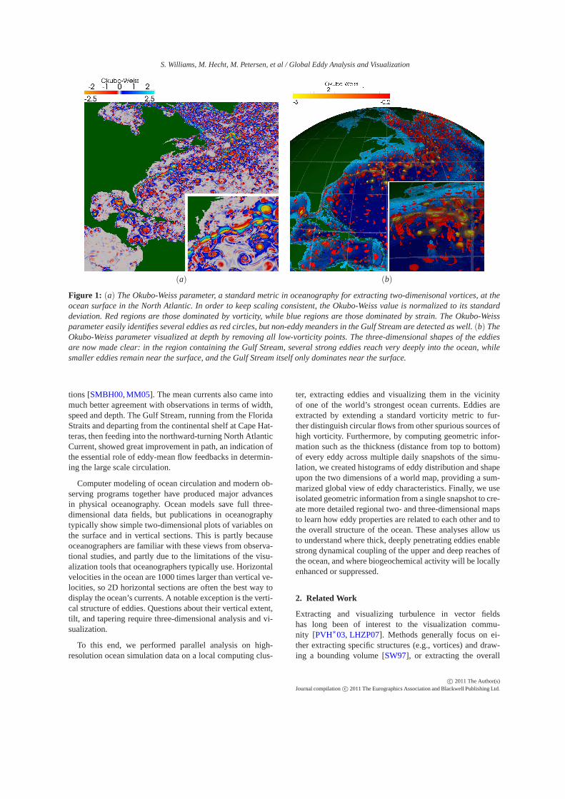
Figure 2: High-vorticity features extracted from the North Atlantic.(a) Features are colored by Okubo-Weiss value, with high-speed water in translucent gray. Where the Gulf Stream turns, additionalnon-eddy but high-vorticity features appear. We wouldlike to filter out these spurious features.(b) The same features, colored based on the angle each point’s velocity vector makeswith an east-pointing vector. Angles are discretized into four domains: angles between east and north (0◦ and 90◦, coloredpurple), north to west (90◦ to 180◦, green), west to south (180◦ to 270◦, yellow), and south to east (270◦ to 360◦, red). Featuresthat are definitely eddies contain a nearly equal mixture of all four angle domains, while meanders move primarily in one ortwo directions and are dominated by one or two angle domains.(c) To use angle domains as a discriminator, we determine foreach high-vorticity feature what percentage of its total volume is flowing in each angle domain. We consider only the minimum:if the feature is perfectly balanced between the four domains (eddy-like), theminimum percentage of any domain will be25%.If the feature contains no points in a domain (non-eddy), its minimum percentage will be0%. We determined experimentallythat requiring a minimum of8% (colored green) in each domain discriminates well between eddies and spurious high-vorticityfeatures—so features colored green here pass the criterion, while features colored red do not.

topology and visualizing it through glyphs or other prox-ies [HH91, TG09]. For extracting vortex-like structures inparticular, popular methods include finding regions of highvorticity [VV92], streamline geometry [SP00] or, if the dataare available, by looking for regions of low pressure at thecenter of a vortex [BS94].

One can also look for circular behavior in the veloc-ity field directly. Jiang et al look at the problem topologi-cally [JMT02], by looking for neighborhoods in which eachvector in the neighborhood points in a unique directionrange. Similarly, Sood et al [SJBT05] identify eddy centersby passing a 5× 5 kernel of the angles between an east-pointing vector and the tangents of a circle centered in thekernel to find circular flows, then fitting an ellipse over theentire eddy. We employ a similar method to discriminatehigh-vorticity features, to attempt to separate eddies fromnon-eddy features.

In 3D visualization, Zhu and Moorhead [ZM95] extracteddies as a stack of 2D contours and stitch them together toshow their 3D structure in the Pacific Ocean off the coast ofJapan. They develop a new extraction technique, but the re-strictiveness of their method appears to preclude extractingdeep eddies, which have been observed to exist in that re-gion. Grant et al [GEO02] developed a method for fitting asurface to the thermocline—the interface between the upper,well-mixed ocean and the deep, stratified ocean. His visual-

izations show quite clearly the perturbations that eddies cancause in the thermocline.

We employ the Okubo-Weiss parameter [Oku70,Wei91],which is a two-dimensional analogue of theλ2 parame-ter [JH95] often used in three-dimensional flow analysis.That is, both parameters use eigenvalues of the strain and ro-tation components of the velocity gradient tensor to find vor-tices, but due to the very low vertical velocities in the ocean,Okubo-Weiss only considers two-dimensional (north-southand east-west) velocities. The relationship between velocitygradient tensors and vortex properties was studied and vi-sualized in much greater detail [ZYLL09], though for ourpurposes thisλ2 style approximation is sufficient.

Numerous studies of satellite data have quantified thesize and distribution of oceanic eddies, mostly based onconsideration of the Okubo-Weiss parameter. Publishedworks have considered regions including the MediterraneanSea [IFGLFGO06], the Tasman Sea [WAB06], the Gulf ofAlaska [HT08] and the full nearly-global domain of all butthe ice-covered seas [CSSdS07].

An eddy census from satellite data is limited to surfacefeatures, while data from vertical ship-deployed profiles andfixed moorings are sparse and can only capture a very in-complete picture. Ocean models have been used as a meansto study features that are not directly observable at this time,and therefore to fill in our understanding of the oceans. Muchof the knowledge of so-called eddy transports of heat, salt



and nutrients has been derived from the analysis of oceanmodels [JM02,YNQ∗10]. It is important to note that the dis-cussion of eddy transport in the literature generally refersto all transport not explicitly accounted for in the mean flow,which will include any temporal variability in the mean flow,such as the slow meandering of large-scale currents.

Eddies are understood to provide a principal means ofcoupling between the circulations of the upper and deepocean [HL75,HH08]. The vertical structure of eddies is alsounderstood to influence the suppression or enhancement ofbiogeochemical activity through their control over nutrientsupply through the base of the euphotic zone (the zone overwhich light penetration is sufficient to support photosynthe-sis). It has been shown that the effect on nutrient supplyand biological activity can be of opposite sign depending onwhether the eddy is a thick one of low vertical mode struc-ture or a thin one of higher vertical mode [AMM ∗10], moti-vating our classification of eddies into thick and thin.

3. Methods

Our analysis of eddies focuses on data generated by LosAlamos National Laboratory’s Parallel Ocean Program(POP) [SDM92] in the context of a global ocean simula-tion with grid resolution of approximately110

◦

. As explainedin [MBH∗08, MBP10], the horizontal grid follows lines oflatitude and longitude in the southern hemisphere, where thelandmass of the Antarctic continent prevents the singularityin latitudinal spacing that occurs at the South Pole (where allgrid points would share the same southern neighbor, turningrectangular grid cells into triangles) from imposing an oth-erwise severe time step limitation on the finite volume dis-cretization of the ocean model. In the northern hemisphere,where the northern pole is in the middle of an ocean basin, amore complex discretization is used in order to maintain rel-atively uniform grid cell areas with horizontal aspect ratiosthat do not deviate greatly from one. This is accomplishedusing a tripole grid, in which two North Poles are used in-stead, with one located in Canada and the other in Siberia. Insuch a grid, the top row of points forms a line from one poleto the other and back again, and any degenerate cells occuron land and are ignored by the simulation.

Oceanic flows take on extreme aspect ratios when con-sidered in three dimensions, with horizontal scales being or-ders of magnitude larger than characteristic vertical scales.Whereas 1

10◦

, or approximately 10 km, is considered ex-tremely fine horizontal resolution, the vertical resolution ismuch higher, with grid spacing on the order of 10 m near thesurface, reaching 250 m in the deep ocean, with a smoothtransition between. The model output is then a rectilineargrid of size 3600×2400×42. These data comprise approx-imately 1.4 GB per floating-point variable per daily snap-shot, so all our visualization and analysis was done on alocal thirty-two core cluster primarily using the visualiza-tion toolkit ParaView. We consider two input variables from

the simulation, comprising the two components of horizon-tal velocity. The vertical velocity does not contribute signifi-cantly to the relative vorticity, being several orders of magni-tude smaller in scale than the horizontal velocity, as is char-acteristic of geophysical flows. Any points that lie in landare assigned a special value of−1034 in all fields, so thebathymetry (a depth map of the bottom of the ocean) can bereadily inferred.

While the details of the grid are specific to a run of POP—the simulation code supports different methods for remov-ing the northern pole singularity, like keeping a single NorthPole but moving it so it lies in Canada—one of the inputsto the POP run (that is similarly available as input to us) isa mapping from grid coordinates to longitude and latitude.The mapping is simply a two-dimensional rectilinear grid ofsize 3600×2400, noting that all points at a particular(i, j)grid coordinate (i.e., at any depth) share the same longitudeand latitude. This creates a spherical coordinate system oflongitude, latitude, andr as the distance from the center ofthe Earth (computed as the radius of the Earth, 6,371 km,minus the depth of the point in the simulation grid) that canbe easily transformed into Cartesian coordinates for makingthe Earth-like visualizations in figures1 and2. In these vi-sualizations, depth is exaggerated by a factor of 50, becausewith three orders of magnitude separating the radius of theEarth (6,371 km) from the maximum depth of POP (about6 km), depth-dependent features (including the bathymetryof the ocean) are imperceptibly small without exaggeration.

3.1. Eddy Extraction

We begin with one of the ocean community’s canonicalmethods for identifying eddies: the Okubo-Weiss param-eter. We chose to start with this metric because, while itcertainly is not the only means of identifying vortical fea-tures, its popularity among oceanographers puts this work ina context that can be immediately understood by membersof the ocean community. In general, this parameter dividesthe ocean into regions dominated by vorticity, regions dom-inated by strain or deformation, and a background whereneither effect is dominant. Regions dominated by vorticityare potentially eddies, though vorticity dominance can becaused by other effects, such as sharp turns in the mean flow.Mathematically, the Okubo-Weiss parameter is defined as:

OW= s2n+s2

s −ω2 (1)

Here,sn is normal strain (currents pushing against eachother),ss is shear strain (currents running in opposite direc-tions past each other), andω is vorticity (currents moving incircles). These three variables can be expressed in terms ofvelocity gradients:



sn =∂u∂x

−

∂v∂y

(2)

ss =∂v∂x

+∂u∂y

(3)

ω =∂v∂x

−

∂u∂y

(4)

Here,u refers to the east-west velocity component, andvto the north-south velocity component. Then,x andy are lo-cally east-pointing and north-pointing vectors, respectively.(We assume that within a single grid cell, which is about11km on a side at the equator and smaller at higher latitudes,the curvature of the Earth is negligible. Thus, we considerthe local coordinate system at each simulation point copla-nar with the local manifold of the Earth.) Substituting thesegradients into the original Okubo-Weiss expression providesan equation that can be solved solely from velocity:

OW=

(

∂u∂x

−

∂v∂y

)2

+

(

∂v∂x

+∂u∂y

)2

−

(

∂v∂x

−

∂u∂y

)2

(5)

Being defined only in terms of velocity gradients, theOkubo-Weiss parameter has the advantage of being entirelylocal and as a result it scales well to large data. A first ap-proach to visualizing the Okubo-Weiss parameter might beto consider the parameter solely in terms of positive (strain-dominated) and negative (vorticity-dominated) domains, butfor numbers close to zero the parameter is dominated bynoise. To select only vorticity-dominated features, then, weneed to apply a threshold to only retain points with negativeOkubo-Weiss values, but due to the parameter being noisyfor very low values, the threshold should be nonzero. Theconvention in the ocean community is to divide the Okubo-Weiss value by its standard deviation (normalizing it suchthat−1 is one standard deviation left of the mean) to providerelatively data-independent scaling of its values, and onlyconsider a data point meaningful if it is at least 0.2 standarddeviations from 0 (i.e., remove all points with Okubo-Weissabove−0.2). We follow this convention, to ensure that ourstarting point for eddy analysis is consistent with the base-line assumptions of prior oceanographic studies of eddies.

The Okubo-Weiss parameter is plotted at the ocean sur-face in Figure1a. For this study we are interested in eddiesas discrete entities (i.e., seeing the strict boundary of eddiesaccording to our definition), so we believe volume renderingwould be inappropriate as a visualization technique. Insteadwe employ a threshold to keep only points with negativeOkubo-Weiss values at least 0.2 standard deviations from 0,and render them as solid cubes. We further place these ex-tracted eddies on a bathymetric map also extracted from thesimulation data to geographically orient viewers and to showthe interaction between deep eddies and the ocean floor. The

resulting visualization is shown for the North Atlantic’s GulfStream in Figure1b.

From this point forward, eddies (or more precisely, high-vorticity features) are defined as connected components ofpoints that all have Okubo-Weiss values below−0.2 stan-dard deviations. Considering that POP lies on a rectilineargrid, we define two points as neighbors if their voxels (theactual volume the points represent) share a face. More col-loquially, this is six-way adjacency: each interior point hassix neighbors, so if a point is indexed by(i, j,k), then itsneighbors are(i+1, j,k), (i−1, j,k), (i, j+1,k), (i, j−1,k),(i, j,k+1), and(i, j,k−1).

These pictures indicate that, while the Okubo-Weiss pa-rameter identifies eddies both at and below the surface of theocean, it also identifies high-vorticity features that shouldnot be considered eddies, particularly meanders in the GulfStream and other strong currents around the world, as wellas several small-scale features that we consider noise. Tomitigate this, we have added one more filtering criterion.We compute the angle between each point’s velocity vec-tor and a vector pointing east. These angles are discretizedinto four domains: 0 to 90 degrees (northeast), 90 to 180degrees (northwest), 180 to 270 degrees (southwest), and270 to 360 degrees (southeast). Figure2b shows the samevorticity-dominated features as Figure2a, but recolored toshow the angle domain each point falls within.

Since an eddy is a circular flow, we expect that an eddyshould contain velocity vectors in all four angle domains,and that its center point should be at the intersection of thesefour domains. Indeed, the vorticity-dominated regions of theGulf Stream that are most likely eddies do show a cross-shaped pattern in their angle domains, indicating that thecurrent is circling around the center of the eddy. However,several of the larger meanders also contain all four angle do-mains, either due to making a sufficiently sharp hairpin turn,or by making S-shaped turns. Instead, for using these angledomains to discriminate between eddies and other features,we require that each angle domain make up at least a cer-tain share of the total eddy, as shown in Figure2c. Based onexperimentation, we arrived at a requirement of 8%.

As our eddy extraction was implemented using ParaView,the computation is parallelized by breaking the data apartinto roughly equally-sized blocks. Besides projecting veloc-ity from grid space to world space to correct for the distor-tions introduced by the tripole coordinate system, comput-ing the Okubo-Weiss parameter is primarily dependent oncomputing velocity gradients. We apply central differencingto find approximate gradients, which is a function on up tosix neighbors. In order to further regularize the data acrosstime, we choose the same normalization factor for the entiredata set: the standard deviation of Okubo-Weiss at the oceansurface on the vernal equinox (March 21). We use a singlenormalization factor for all time steps to ensure that the mag-nitude of Okubo-Weiss is directly comparable between time



steps. We then use ParaView’s threshold filter to remove allpoints with Okubo-Weiss above−0.2σ, leaving only high-vorticity features behind. At this point, the angle betweeneach point’s velocity vector and an east-pointing vector iscomputed from simple trigonometry, and discretized intoone of the four domains as above.

After the threshold filter is applied, ParaView automat-ically converts the data to an unstructured grid with thesame connectivity implicit in the rectilinear grid and, sincethe threshold automatically breaks connectivity between un-connected eddies (because the points connecting the eddieshave been removed), eddies can be identified with a breadth-first search. The final implementation consideration is thatin dividing the data, it is quite likely for some eddies to besplit across two processes. In that case, since a breadth-firstsearch in one process would not automatically cross the pro-cess boundary, the split eddy would be represented as twoindependent eddies, causing the eddy to be either double-counted, or more likely, making it too dominant in one ortwo angle domains and fail to pass our angle criterion.

There are two obvious solutions: employ message passingbetween the processes, or have the boundaries overlap by atleast the size of the largest eddy. We opted for the latter so-lution, since then each eddy automatically resides entirely inat least one process. Specifically, each process has a certainblock assigned to it, with points assigned uniquely to blocksand all points in exactly one block, and each process alsotakes an overlap region into its neighboring blocks such that,while each point is uniquely claimed, it can appear in theoverlap region of up to three other processes. Finally, sincethat implies that an eddy in the overlap region will reside inpart or in whole in at least two processes, a process is onlyallowed to claim an eddy if the point with minimum Okubo-Weiss is not in its overlap region. The only caveat to this def-inition is that it assumes a unique minimum Okubo-Weissvalue per eddy, further subject to the vagaries of floating-point numbers, though floating-point imprecision has not ap-peared to be a problem in practice. While it might also ap-pear to be a problem that one process might not have thepoint with minimum Okubo-Weiss value in either its mainblock or its overlap zone, we assume that the overlap zone isat least as large as the largest eddy. If a point from an eddyis not contained anywhere in the data available to a specificprocess, then the eddy must touch a border and therefore re-side entirely in the overlap zone, so it cannot be claimed bythat process.

3.2. Census and Analysis

In addition to visualizing ocean eddies directly, we also de-veloped a capability to analyze the distribution, size, thick-ness, and depth of eddies around the world. We consider thefollowing computed quantities for each eddy:

• Volume: computed as sum of the volumes of all voxels in

the eddy, with voxels approximated as cubes (though inreality they would be rectangular solid angles of a spheri-cal shell)

• Radius: we consider the radius (the radial extent of aneddy in a latitude-longitude manifold, i.e., in a plane nor-mal to the surface of the Earth) with respect to the depthcontaining the most negative (i.e., strongest) Okubo-Weiss value; at this depth, the radius is approximated bycomputing the area of the eddy at that depth as the sumof the areas of all voxels (computed as the longitudinalextent times the latitudinal extent), then by assuming theeddy is a circle at this depth, takingr =

√

A/π• Thickness: computed as the maximum difference between

the depths of any two points in the eddy• Vorticity sign: positive if at least half the points in the

eddy have positive vorticity (spin counterclockwise), andnegative otherwise

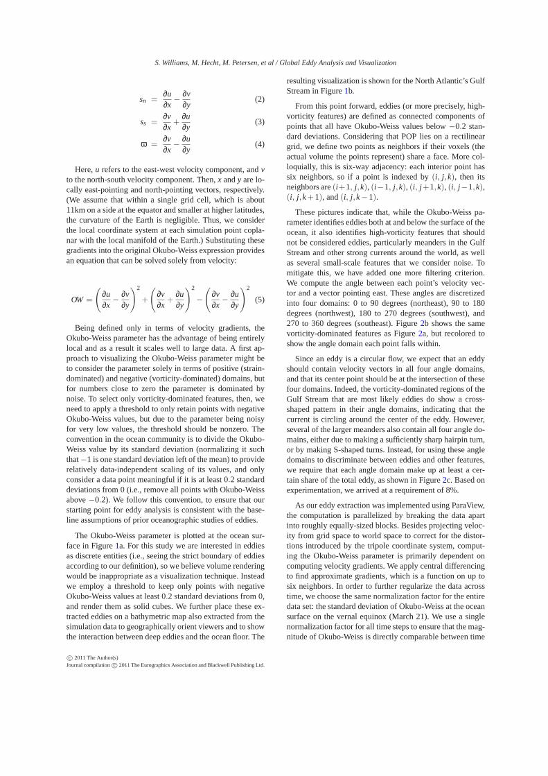
Visualizations like those in the previous section are onlyuseful for looking at snapshots of isolated regions of theocean, due to the density of information being displayed.Here we synthesize 350 global snapshots of daily data to cre-ate an eddy census database in order to study the statisticaldistributions of eddy metrics.

To generate the census, the world is broken into bins 1◦

on each edge. One statistic we highlight is a count: for eachsnapshot, the number of eddies in each bin is counted, theneach bin’s count is averaged across the 350 available dailysnapshots. This census, in Figure3c, shows strong eddyactivity in the Gulf Stream in the western Atlantic Ocean,the Kuroshio Current in the western Pacific Ocean, andthe Antarctic Circumpolar Current ringing Antarctica in theSouthern Ocean. Additionally, because of the simplicity ofthe statistics in this image, it can easily be qualitatively com-pared to observational data to confirm its validity. In Figures3a and3b we use model and satellite altimetry data to de-rive sea surface height variability, or, the difference betweeninstantaneous and averaged sea surface height. The princi-ple observation is that eddies cause bulges on the surfaceof the ocean. Averaging the sea surface height over a largeamount of time removes the temporary bulges caused by ed-dies (providing the sea surface height due to mean flow).Then, the difference between the average and instantaneoussea surface height highlights behavior not attributable to themean flow, e.g., eddies. Using this approach shows regionsof observed strong surface eddy activity, which correspondfairly well to the eddy activity regions found by our census.

The surface characteristics of eddies are well known fromsatellite observations, but the depth of penetration has beenless adequately observed. With model data we can measureaverage eddy thickness, or the distance from the top of theeddy to the bottom. Figure3d reveals several thick eddies inthe midst of the Gulf Stream, Kuroshio Current, and Antarc-tic Circumpolar Current. Focusing on the Atlantic, there aresignificant numbers of eddies with depths on the order of



(a) (b)

(c) (d)

Figure 3: Sea surface height variability in centimeters, defined as the root mean square of the difference between the instanta-neous height of the sea surface and its time-mean, can be used as a proxy measurement for eddy activity. To compare model toobservational data directly, we first show sea surface height variability from(a) POP ocean model data and(b) observationaldata from the AVISO processing of satellite altimetry. In these images, the simulation shows exceptionally good agreement toobservation.(c) Our global eddy census, showing the average number of eddies per1◦ of latitude and longitude, averagedacross 350 daily snapshots. Note that the color bar of(c) is reversed relative to that of(a) and(b). Relating the numerical den-sity of eddies in(c) to sea surface height variability, both measures indicate high levels of eddyactivity in the same locations.(d) Average eddy thickness in meters as a function of latitude and longitude. We use thickness to refer to the distance from thetop of an eddy to the bottom. Notably, thick eddies only have a significant signal in the regions of the same three big currents,the Gulf Stream, Kuroshio Current, and Antarctic Circumpolar Current, where they can get as thick as 5000m.

5000m. This means that some eddies extend from the sur-face of the ocean to the floor, and several more stretch halfthe maximum height of the ocean.

Oceanographers would like to know which eddies are con-fined to the upper ocean, which extend into the deep ocean,and if there are isolated deep eddies without surface features.The upper ocean is well mixed due to wind-induced wavesand turbulence, while the deep ocean is stratified with lit-tle vertical mixing. The thermocline—a surface at the depthwhere temperature changes more rapidly—lies somewherebetween these two regions of lower vertical temperature gra-dient, and serves as a depth to separate shallow eddies fromdeep eddies in our analysis.

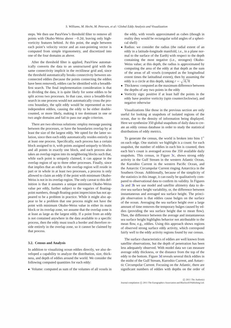
Figure4a shows a skeletonized view of the region of thenorthwest Atlantic we identified from Figure3d as likely tocontain thermocline-penetrating eddies. Eddy skeletons aredrawn as a cylinder vertically spanning the thickness of theeddy (so the top of the cylinder is at the same depth as thehighest point in the eddy, and the bottom of the cylinder is atthe same depth as the lowest point in the eddy), and the cylin-der passes through the most vortical point in the eddy (wherethe Okubo-Weiss value is most negative). The cylinders aredrawn with fixed radius to avoid providing overwhelming

amounts of information, as this visualization contains all theinformation we need to address the question under consider-ation. Even from this simplified view it is visually apparentthat there are several eddies beginning near the surface of theocean and extending down quite far, but to make the relation-ship more explicit, we created a two-dimensional map show-ing where thermocline-penetrating eddies occur. Eddies thatpenetrate the thermocline, meaning that they begin above thethermocline and end below it, are shown as blue squaresif they spin counterclockwise, and red squares if they spinclockwise. Eddies entirely above or below the thermoclineare represented by gray diamonds. For this map, we use anestimate of the thermocline depth of 700m [AMM ∗10].

4. Results

Our results were reviewed by three Los Alamos NationalLaboratory scientists specializing in ocean modeling—Matthew Hecht, Mark Petersen, and Mat Maltrud—whodrew a number of insights from these visualizations. Theirconsideration of results begins with Figure2c, wherediscrimination has been performed in order to separatemesoscale eddies from other high-vorticity features. In thisview of the northwest Atlantic the deeper eddies tend to be



(a) (b)

Figure 4: (a) Skeletonized view of the eddy field in the northwest Atlantic, from−80◦ to −30◦ longitude and20◦ to 50◦

latitude. Eddies are pictured as blue or red cylinders of vertical extent, withblack lines projecting subsurface eddies onto theocean surface to aid in visual alignment. Blue eddies have positive vorticity (counterclockwise spin), while red eddies havenegative vorticity (clockwise spin). The green translucent layer approximates the thermocline.(b) Two-dimensional map of thesame eddy field. Eddies that penetrate the thermocline (i.e., that have their minimum depth above the thermocline and theirmaximum depth below) are represented as colored boxes; these are theeddies that can couple the upper and deep ocean.Coloration is the same used in the skeletonized view: blue for counterclockwise and red for clockwise. Eddies that exist entirelyabove or below the thermocline are gray diamonds. For this region of the Atlantic, the thermocline is at about 700m [AMM∗10].

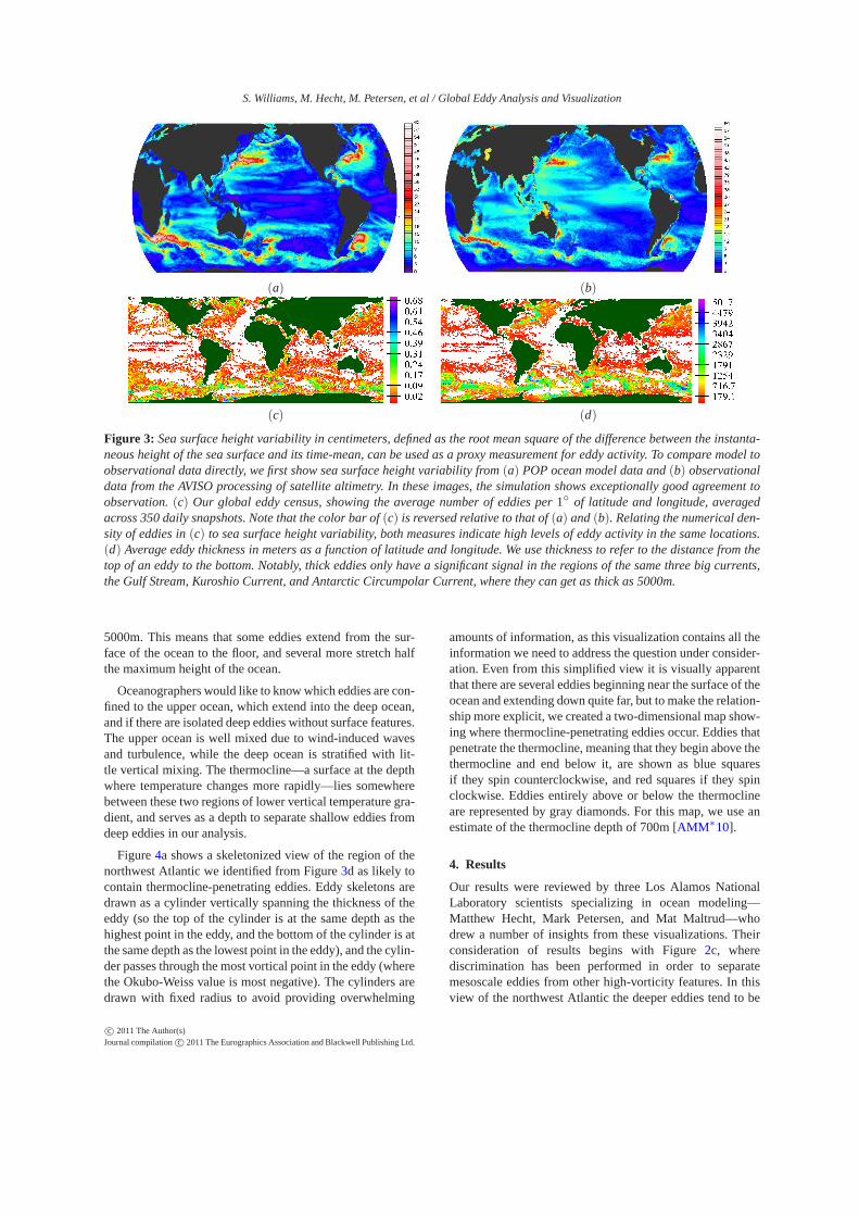
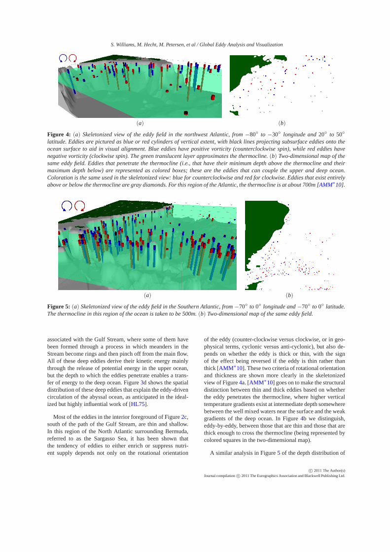
(a) (b)

Figure 5: (a) Skeletonized view of the eddy field in the Southern Atlantic, from−70◦ to 0◦ longitude and−70◦ to 0◦ latitude.The thermocline in this region of the ocean is taken to be 500m.(b) Two-dimensional map of the same eddy field.

associated with the Gulf Stream, where some of them havebeen formed through a process in which meanders in theStream become rings and then pinch off from the main flow.All of these deep eddies derive their kinetic energy mainlythrough the release of potential energy in the upper ocean,but the depth to which the eddies penetrate enables a trans-fer of energy to the deep ocean. Figure3d shows the spatialdistribution of these deep eddies that explain the eddy-drivencirculation of the abyssal ocean, as anticipated in the ideal-ized but highly influential work of [HL75].

Most of the eddies in the interior foreground of Figure2c,south of the path of the Gulf Stream, are thin and shallow.In this region of the North Atlantic surrounding Bermuda,referred to as the Sargasso Sea, it has been shown thatthe tendency of eddies to either enrich or suppress nutri-ent supply depends not only on the rotational orientation

of the eddy (counter-clockwise versus clockwise, or in geo-physical terms, cyclonic versus anti-cyclonic), but also de-pends on whether the eddy is thick or thin, with the signof the effect being reversed if the eddy is thin rather thanthick [AMM ∗10]. These two criteria of rotational orientationand thickness are shown more clearly in the skeletonizedview of Figure4a. [AMM ∗10] goes on to make the structuraldistinction between thin and thick eddies based on whetherthe eddy penetrates the thermocline, where higher verticaltemperature gradients exist at intermediate depth somewherebetween the well mixed waters near the surface and the weakgradients of the deep ocean. In Figure4b we distinguish,eddy-by-eddy, between those that are thin and those that arethick enough to cross the thermocline (being represented bycolored squares in the two-dimensional map).

A similar analysis in Figure5 of the depth distribution of



eddies in the Southern Ocean, where the powerful Antarc-tic Circumpolar Current circles the Earth nearly unimpededby land masses, shows a remarkable concentration of deepeddies that pass our detection criteria to the bottom of theocean. It should be noted that for numerical reasons (i.e.,how many points are required to get 8% in each angle do-main relative to the total number of points) our detectioncriteria is stricter in a relative sense in the deep ocean, ascompared with the upper ocean, because deep ocean veloc-ities tend to be smaller. It seems likely that these particu-larly intense eddies have been “pinched off” as meanders inthe flanks of the Current. The formation process will be ex-amined once our techniques have been extended in a robustway to the tracking of individual three-dimensional eddiesthrough time.

The great abundance of thick eddies in the SouthernOcean, along the path of the Antarctic Circumpolar Cur-rent, is also very apparent in Figure3d. It has recently beenargued, again based on idealized study, that the eddies ofthe Southern Ocean set the stratification of the much of theWorld Ocean [WC10]. Our visualizations show that there isa vast array of deep eddies spanning the southern extremes ofthe Pacific, Atlantic and Indian sectors, capable of exertingcontrol over the mid-depth stratification of the World Ocean.

Another area in which particularly deep-reaching eddiesappear in Figure3d is where the westward-flowing Agul-has Current has its “retroflection.” This occurs off the south-ern tip of Africa, where most of the waters of the Agul-has Current reverse course to become swept up with theeastward-flowing Antarctic Circumpolar Current, and deepeddies sporadically break off of the powerful Agulhas Cur-rent. This sends masses of Indian Ocean waters spinningoff into and across the South Atlantic where they modulatethe strength of the Atlantic overturning circulation [BBL08].The Gulf Stream region is also closely associated with theoverturning circulation, with its downstream manifestation,the North Atlantic Current, believed to have taken a differentcourse at the time of the Last Glacial Maximum [RMM95],and this is another region of notably deep eddies. This isalso a region in which a particularly vigorous deep circu-lation appears to be driven by vertical momentum transferthrough the eddy field. In turn, the deep circulation interactsstrongly with the circulation of the upper ocean, controllingthe path of the Gulf Stream, in a delicate and entirely mu-tual interaction between upper and lower components of thecirculation [HH08].

5. Conclusion

The complete role of deep, thermocline-penetrating eddies isnot currently well understood. Partly this is because observa-tional data at depth are sparse, and global ocean simulationshave only recently reached the resolutions required to reli-ably resolve eddies. We began addressing this by extractingeddies from a tenth-degree global ocean simulation, start-

ing from the standard Okubo-Weiss parameter. Because theOkubo-Weiss parameter identifies any feature where vortic-ity dominates strain, we created a new criterion to select forcircular, more eddy-like vorticity features. From there, wegathered statistical data about the global eddy field across350 daily snapshots and visualized them in a summarizedworld map of characteristics and distributions, and usedstatistics from a single snapshot to make detailed geograph-ical and correlative visualizations of the eddies’ properties.

To this end, we intend to expand our analytical capabil-ities to include eddy tracking over time, and to allow formore extensive three-dimensional consideration of correla-tions with additional variables including temperature, salin-ity, potential density and enstrophy.

Acknowledgements

This work was supported by the Department of Energy(DOE) Office of Science (OSC) Biological and Environ-mental Research (BER) Climate Visualization Program, theLANL-UC Davis Materials Design Institute, and in part byNSF grant CCF-0702817. Finally, we thank the membersof the Institute for Data Analysis and Visualization (IDAV),Department of Computer Science, UC Davis, and the Ap-plied Computer Science group at Los Alamos National Lab-oratory.

References

[AMM ∗10] ANDERSON L. A., M CGILLICUDDY , JR. D. J.,MALTRUD M. E., LIMA I. D., DONEY S. C.: Impact of eddy-wind interaction on eddy demographics and phytoplankton com-munity structure in a model of the North Atlantic Ocean.Dyn.Atmos. Oceans(2010), submitted.4, 7, 8

[BBL08] B IASTOCH A., BÖNING C. W., LUTJEHARMS J.: Ag-ulhas leakage dynamics affects decadal variability in Atlanticoverturning circulation.Nature 456(2008), 489–492.9

[BH89] BRYAN F., HOLLAND W.: A high-resolution simulationof the wind- and thermohaline-driven circulation in the North At-lantic Ocean. InProceedings of the ’Aha Huliko’a HawaiianWinter Workshop, Muller P., Henderson D., (Eds.), Hawaii Inst.Geophys. Spec. Publ. U. Hawaii, 1989, pp. 99–115.1

[Bry69] BRYAN K.: A numerical method for the study of thecirculation of the World Ocean.J. Comput. Phys.4(1969), 347—376. 1

[BS94] BANKS D. C., SINGER B. A.: Vortex tubes in turbulentflows: identification, representation, reconstruction. InVIS ’94:Proceedings of the conference on Visualization ’94(Los Alami-tos, CA, USA, 1994), IEEE Computer Society Press, pp. 132–139. 3

[CSSdS07] CHELTON D. B., SCHLAX M. G., SAMELSON

R. M., DE SZOEKE R. A.: Global observations of large oceaniceddies.Geophysical Research Letters 34, L15606 (2007), 5.3

[FRA91] FRAM GROUP: An eddy-resolving model of the South-ern Ocean.EOS Trans. AGU72(1991), 169–175.1

[FS96] FU L. L., SMITH R. D.: Global ocean circulation fromsatellite altimetry and high-resolution computer simuation.Bull.Amer. Meteorol. Soc.11, 77 (1996), 2625–2636.1



[GEO02] GRANT J., ERLEBACHER G., O’BRIEN J.: Casestudy: Visualizing ocean flow vertical motions using lagrangian-eulerian time surfaces. InVisualization, 2002. VIS 2002. IEEE(Nov. 2002), pp. 529 –532.3

[HH91] HELMAN J. L., HESSELINK L.: Visualizing vector fieldtopology in fluid flows.IEEE Comput. Graph. Appl. 11, 3 (1991),36–46.3

[HH08] HURLBURT H. E., HOGAN P. J.: The Gulf Stream path-way and the impacts of the eddy-driven abyssal circulation andthe Deep Western Boundary Current.Dyn. Atmos. Oceans 45(2008), 71–101.4, 9

[HL75] HOLLAND W. R., LIN L. B.: On the generation ofmesoscale eddies and their contribution to the oceanic generalcirculation. I. A preliminary numerical experiment.J. Phys.Oceanogr.5, 4 (1975), 642 – 57.4, 8

[HT08] HENSON S. A., THOMAS A. C.: A census of oceanicanticyclonic eddies in the gulf of alaska.Deep Sea Research PartI: Oceanographic Research Papers 55, 2 (2008), 163 – 176.3

[IFGLFGO06] ISERN-FONTANET J., GARCÍA-LADONA E.,FONT J., GARCÍA-OLIVARES A.: Non-gaussian velocity proba-bility density functions: An altimetric perspective of the mediter-ranean sea.J. Phys. Oceanogr.36, 11 (2006), 2153 – 2164.3

[JH95] JEONG J., HUSSAIN F.: On the identification of a vortex.Journal of Fluid Mechanics 285(1995), 69–94.3

[JM02] JAYNE S. R., MAROTZKE J.: The oceanic eddy heattransport*. Journal of Physical Oceanography 32, 12 (2002),3328–3345.4

[JMT02] JIANG M., MACHIRAJU R., THOMPSON D.: A novelapproach to vortex core region detection. InProceedings of thesymposium on Data Visualisation 2002(Aire-la-Ville, Switzer-land, Switzerland, 2002), VISSYM ’02, Eurographics Associa-tion, pp. 217–ff.3

[LBM02] L EACH H., BOWERMAN S. J., MCCULLOCH M. E.:Upper-ocean eddy transports of heat, potential vorticity,and vol-ume in the northeastern north atlantic—“vivaldi 1991”.Journalof Physical Oceanography 32, 10 (2002), 2926–2937.1

[LHZP07] LARAMEE R., HAUSER H., ZHAO L., POST F.:Topology-based flow visualization, the state of the art. InTopology-based Methods in Visualization, Hauser H., HagenH., Theisel H., (Eds.), Mathematics and Visualization. SpringerBerlin Heidelberg, 2007, pp. 1–19. 10.1007/978-3-540-70823-0_1. 2

[MBH∗08] MALTRUD M., BRYAN F., HECHT M., HUNKE E.,IVANOVA D., MCCLEAN J., PEACOCK S.: Global ocean mod-elling in the eddying regime using POP.CLIVAR Exchanges 44,1 (January 2008), 5–8. (unpublished manuscript).4

[MBP10] MALTRUD M., BRYAN F., PEACOCK S.: Boundary im-pulse response functions in a century-long eddying global oceansimulation.Environmental Fluid Mechanics 10, 1-2 (APR 2010),275–295.4

[MM05] M ALTRUD M. E., MCCLEAN J. L.: An eddy resolving1/10◦ ocean simulation.Ocean Modelling8, 1–2 (2005), 31–54.2

[MPH∗07] MATHIS J. T., PICKART R. S., HANSELL D. A.,KADKO D., BATES N. R.: Eddy transport of organic carbon andnutrients from the Chukchi Shelf: Impact on the upper haloclineof the western Arctic Ocean.Journal of Geophysical Research(Oceans) 112, C11 (May 2007), 5011.1

[Oku70] OKUBO A.: Horizontal dispersion of floatable parti-cles in the vicinity of velocity singularities such as convergences.Deep Sea Research and Oceanographic Abstracts 17, 3 (1970),445 – 454.3

[PVH∗03] POST F. H., VROLIJK B., HAUSER H., LARAMEE

R. S., DOLEISCH H.: The state of the art in flow visualisation:Feature extraction and tracking.Computer Graphics Forum 22,4 (2003), 775–792.2

[RMM95] ROBINSON S. G., MASLIN M. A., M CCAVE I. N.:Magnetic-susceptibility variations in Upper Pleistocenedeep-seasediments of the NE Atlantic – Implications for ice rafting andpaleocirculation at the Last Glacial Maximum.Paleoceanogra-phy 10, 2 (1995), 221 – 250.9

[SDM92] SMITH R. D., DUKOWICZ J. K., MALONE R. C.: Par-allel ocean general circulation modeling.Physica D: NonlinearPhenomena60(1992), 38—61.4

[SJBT05] SOOD V., JOHN B., BALASUBRAMANIAN R., TAN-DON A.: Segmentation and tracking of mesoscale eddies in nu-meric ocean models. InImage Processing, 2005. ICIP 2005.IEEE International Conference on(September 2005), vol. 3,pp. III – 469–72.3

[SMBH00] SMITH R. D., MALTRUD M. E., BRYAN F. O.,HECHT M. W.: Numerical simulation of the North AtlanticOcean at1

10◦. J. Phys. Oceanogr.30(2000), 1532–1561.2

[SP00] SADARJOEN I. A., POST F. H.: Detection, quantification,and tracking of vortices using streamline geometry.Computers& Graphics 24, 3 (2000), 333 – 341.3

[SW97] SILVER D., WANG X.: Tracking and visualizing turbu-lent 3d features.Visualization and Computer Graphics, IEEETransactions on 3, 2 (apr. 1997), 129 –141.2

[TG09] TRICOCHE X., GARTH C.: Topological methods for vi-sualizing vortical flows. InMathematical Foundations of Scien-tific Visualization, Computer Graphics, and Massive Data Explo-ration, Farin G., Hege H.-C., Hoffman D., Johnson C. R., PolthierK., Rumpf M., (Eds.), Mathematics and Visualization. SpringerBerlin Heidelberg, 2009, pp. 89–107. 10.1007/b106657_5.3

[VLF08] VOLKOV D. L., LEE T., FU L.: Eddy-induced merid-ional heat transport in the ocean.Geophys. Res. Lett.35(Oct.2008), 20601–+.1

[VV92] V ILLASENOR J., VINCENT A.: An algorithm for spacerecognition and time tracking of vorticity tubes in turbulence.CVGIP: Image Understanding 55, 1 (1992), 27 – 35.3

[WAB06] WAUGH D. W., ABRAHAM E. R., BOWEN M. M.:Spatial variations of stirring in the surface ocean: A case studyof the tasman sea.J. Phys. Oceanogr.36, 3 (2006), 526 – 542.3

[WC10] WOLFE C. L., CESSI P.: What Sets the Strength of theMiddepth Stratification and Overturning Circulation in EddyingOcean Models?J. Phys. Oceanogr.40, 7 (2010), 1520–1538.9

[Wei91] WEISS J.: The dynamics of enstrophy transfer in two-dimensional hydrodynamics.Physica D: Nonlinear Phenomena48, 2-3 (1991), 273 – 294.3

[YNQ∗10] YIM B. Y., NOH Y., QIU B., YOU S. H., YOON

J. H.: The vertical structure of eddy heat transport simulatedby an eddy-resolving ogcm.Journal of Physical Oceanography40, 2 (2010), 340–353.4

[ZM95] ZHU Z., MOORHEAD R. J.: Extracting and visualizingocean eddies in time-varying flow fields, 1995.3

[ZYLL09] Z HANG E., YEH H., LIN Z., LARAMEE R.: Asym-metric tensor analysis for flow visualization.Visualizationand Computer Graphics, IEEE Transactions on 15, 1 (January-February 2009), 106 –122.3


visualization and analysis of eddies in a global ocean...

Documents